neutrino oscillations or how we know most of what we know

Neutrino Oscillations

Or how we know most of what we know

June 2005 Steve Elliott, NPSS 2005 2

Outline

• Two-flavor vacuum oscillations

• Two-flavor matter oscillations

• Three-flavor oscillations– The general formalism– The “rotation” matrices


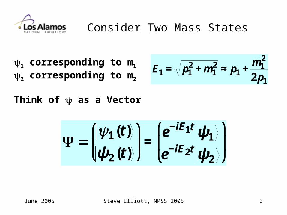
Consider Two Mass States

1 corresponding to m1

2 corresponding to m2

Think of as a Vector

€

Ψ =1(t)

ψ2 (t)

⎛

⎝ ⎜

⎞

⎠ ⎟=

e−iE1t ψ1

e−iE2t ψ2

⎛

⎝ ⎜

⎞

⎠ ⎟

€

E1 = p12 + m1

2 ≈ p1 +m1

2

2 p1


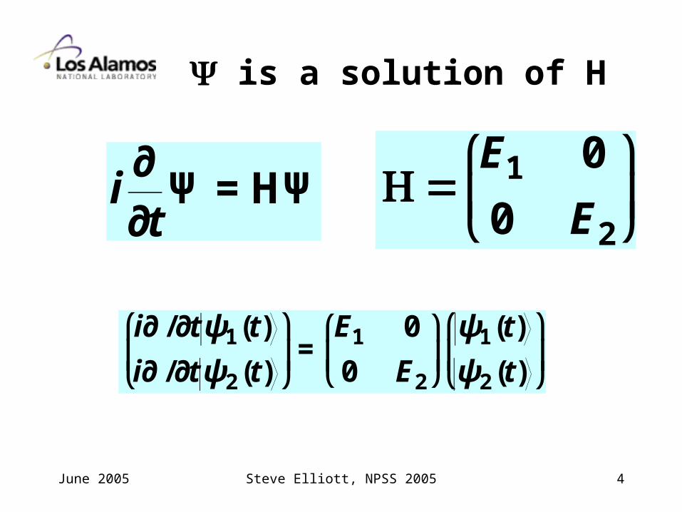
Ψ is a solution of H

€

i∂∂t

Ψ = HΨ

€

H=E1 0

0 E2

⎛

⎝ ⎜

⎞

⎠ ⎟

€

i∂ /∂t ψ1(t)

i∂ /∂t ψ2 (t)

⎛

⎝ ⎜

⎞

⎠ ⎟=

E1 0

0 E2

⎛

⎝ ⎜

⎞

⎠ ⎟ψ1(t)

ψ2 (t)

⎛

⎝ ⎜

⎞

⎠ ⎟


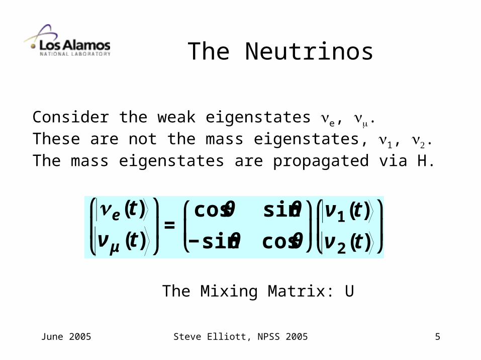
The Neutrinos

Consider the weak eigenstates e, .These are not the mass eigenstates, 1, .The mass eigenstates are propagated via H.

€

e (t)

ν μ (t)

⎛

⎝ ⎜

⎞

⎠ ⎟=

cosθ sinθ

−sinθ cosθ

⎛

⎝ ⎜

⎞

⎠ ⎟ν 1(t)

ν 2 (t)

⎛

⎝ ⎜

⎞

⎠ ⎟

The Mixing Matrix: U


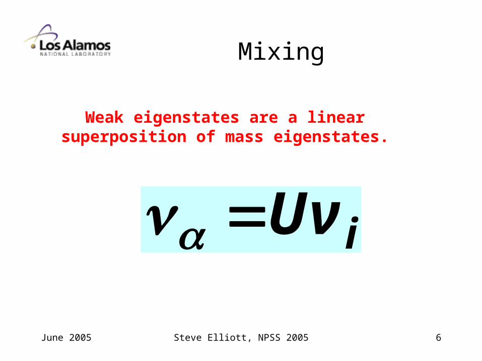
Mixing

Weak eigenstates are a linear superposition of mass eigenstates.

€

α =Uν i


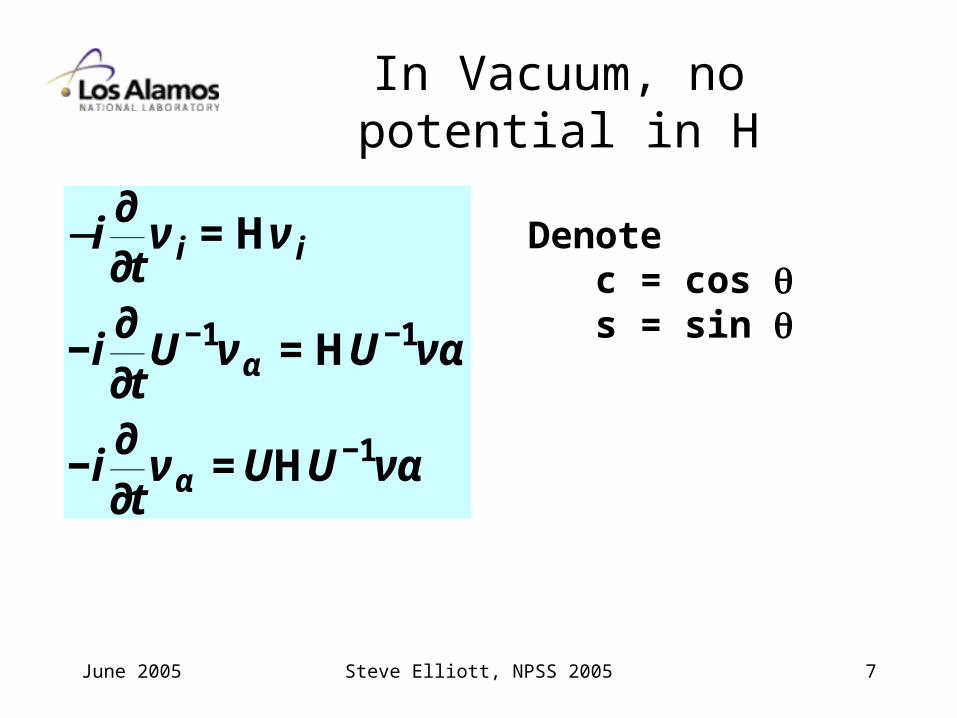
In Vacuum, no potential in H

€

−i∂∂t

ν i = Hν i

−i∂∂t

U−1ν α = HU−1να

−i∂∂t

ν α = UHU−1να

Denote c = cos s = sin


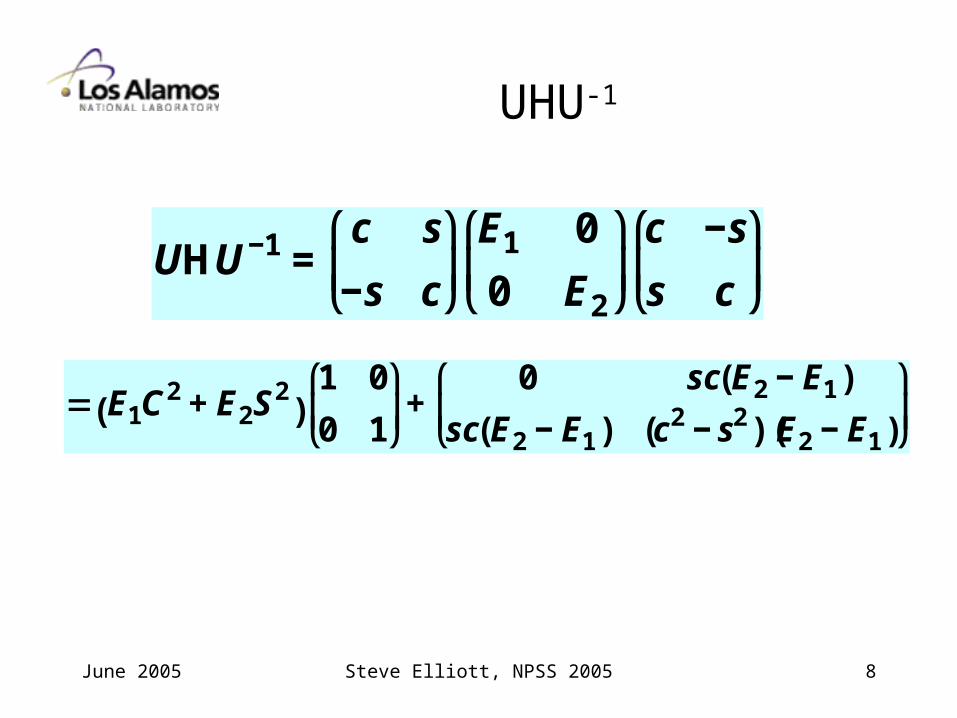
UHU-1

€

UHU−1 =c s

−s c

⎛

⎝ ⎜

⎞

⎠ ⎟E1 0

0 E2

⎛

⎝ ⎜

⎞

⎠ ⎟c −s

s c

⎛

⎝ ⎜

⎞

⎠ ⎟

€

= E1C2 + E2S2( )

1 0

0 1

⎛

⎝ ⎜

⎞

⎠ ⎟+

0 sc(E2 − E1 )

sc(E2 − E1 ) (c2 − s2 )(E2 − E1 )

⎛

⎝ ⎜

⎞

⎠ ⎟


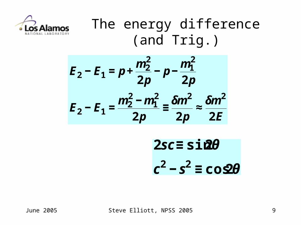
The energy difference (and Trig.)

€

E2 − E1 = p +m2

2

2 p− p −

m12

2 p

E2 − E1 =m2

2 − m12

2 p≡

δm2

2 p≈

δm2

2E

€

2sc ≡ sin2θ

c2 − s2 ≡ cos2θ


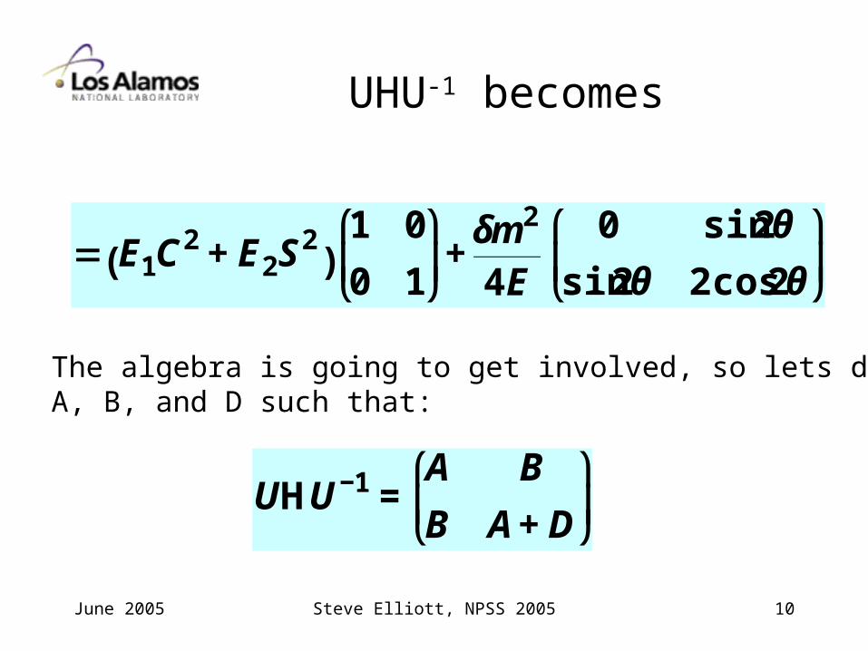
UHU-1 becomes

€

= E1C2 + E2S2( )

1 0

0 1

⎛

⎝ ⎜

⎞

⎠ ⎟+

δm2

4E

0 sin2θ

sin2θ 2cos2θ

⎛

⎝ ⎜

⎞

⎠ ⎟

The algebra is going to get involved, so lets defineA, B, and D such that:

€

UHU−1 =A B

B A+ D

⎛

⎝ ⎜

⎞

⎠ ⎟


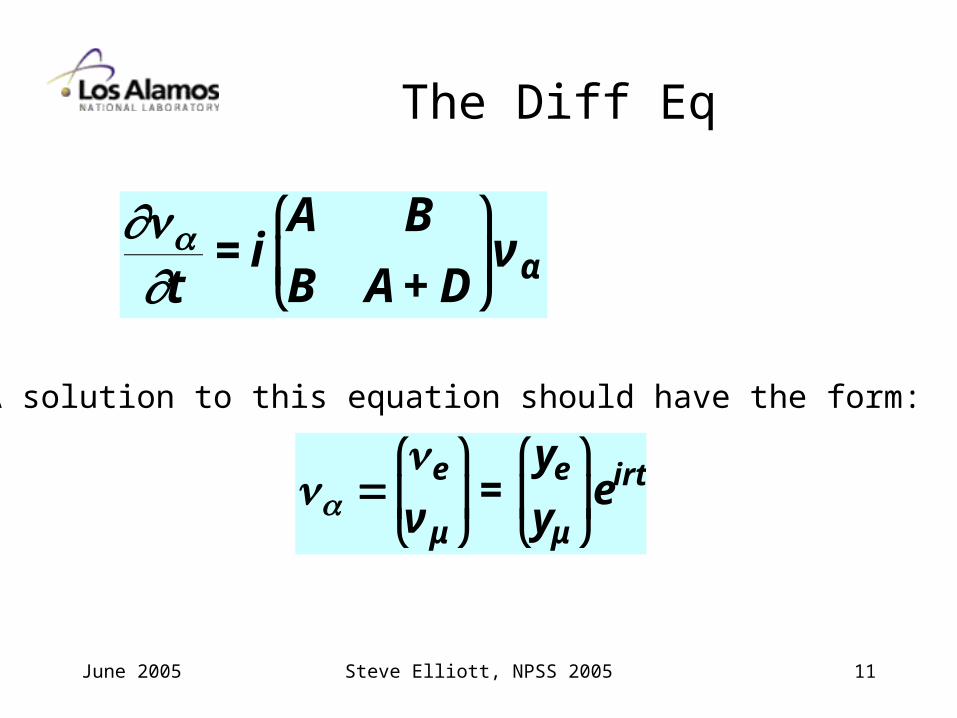
The Diff Eq

€

∂α∂t

= iA B

B A+ D

⎛

⎝ ⎜

⎞

⎠ ⎟ν α

A solution to this equation should have the form:

€

α =e

ν μ

⎛

⎝ ⎜

⎞

⎠ ⎟=

ye

yμ

⎛

⎝ ⎜

⎞

⎠ ⎟eirt


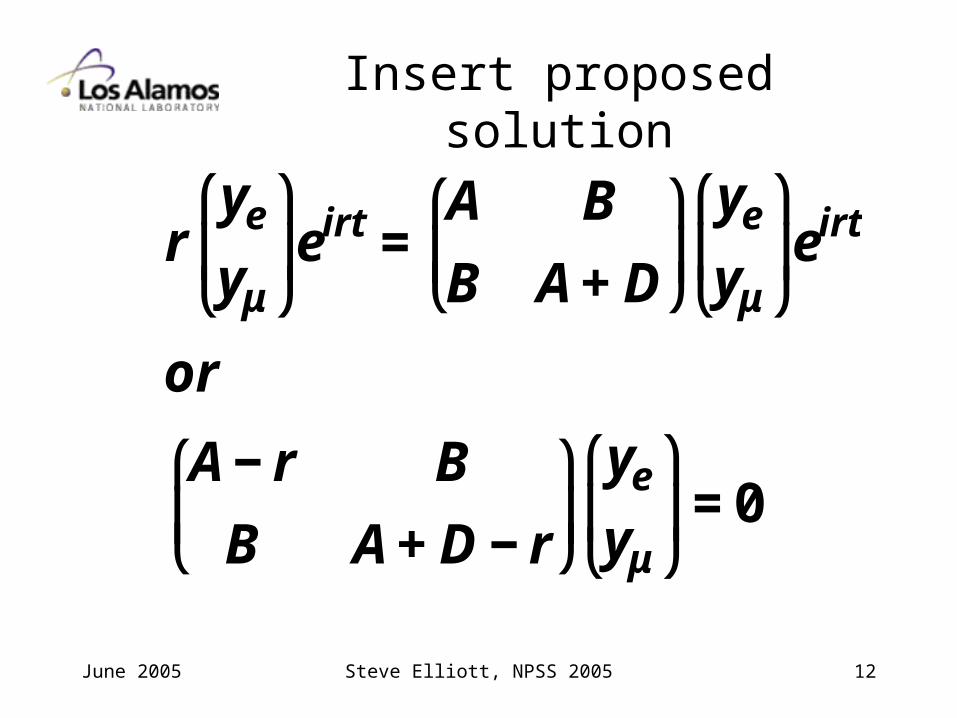
Insert proposed solution

€

rye

yμ

⎛

⎝ ⎜

⎞

⎠ ⎟eirt =

A B

B A+ D

⎛

⎝ ⎜

⎞

⎠ ⎟ye

yμ

⎛

⎝ ⎜

⎞

⎠ ⎟eirt

or

A− r B

B A+ D − r

⎛

⎝ ⎜

⎞

⎠ ⎟ye

yμ

⎛

⎝ ⎜

⎞

⎠ ⎟= 0


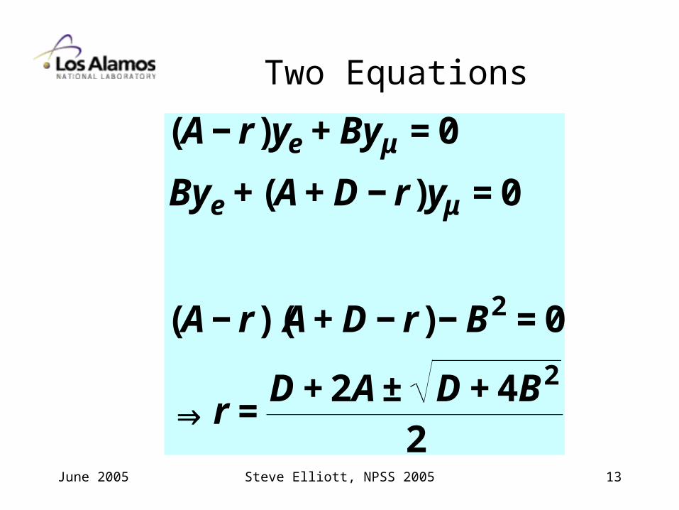
Two Equations

€

(A− r)ye + Byμ = 0

Bye + (A+ D − r)yμ = 0

(A− r)(A+ D − r)− B2 = 0

⇒ r =D + 2A± D + 4B2

2


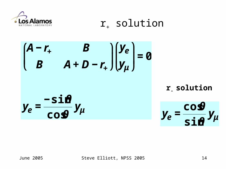
r+ solution

€

A− r+ B

B A+ D − r+

⎛

⎝ ⎜

⎞

⎠ ⎟ye

yμ

⎛

⎝ ⎜

⎞

⎠ ⎟= 0

ye =−sinθcosθ

yμ

r- solution

€

ye =cosθsinθ

yμ


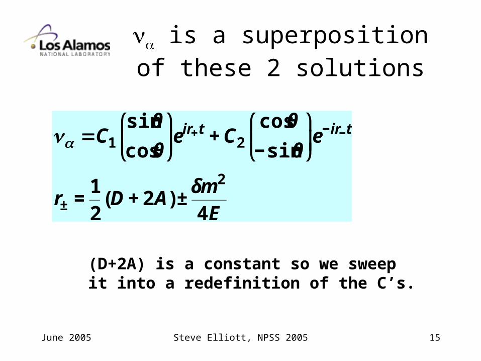
α is a superposition of these 2 solutions

€

α =C1sinθ

cosθ

⎛

⎝ ⎜

⎞

⎠ ⎟e

ir+t + C2cosθ

−sinθ

⎛

⎝ ⎜

⎞

⎠ ⎟e

−ir−t

r± =12

(D + 2A)±δm2

4E

(D+2A) is a constant so we sweep it into a redefinition of the C’s.


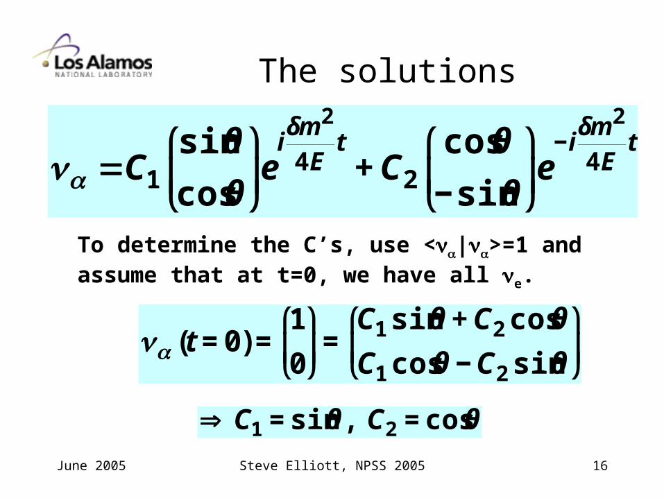
The solutions

€

α =C1sinθ

cosθ

⎛

⎝ ⎜

⎞

⎠ ⎟e

iδm2

4Et

+ C2cosθ

−sinθ

⎛

⎝ ⎜

⎞

⎠ ⎟e

−iδm2

4Et

To determine the C’s, use <α|α>=1 and assume that at t=0, we have all e.

€

α (t = 0) =1

0

⎛

⎝ ⎜

⎞

⎠ ⎟=

C1 sinθ + C2 cosθ

C1 cosθ − C2 sinθ

⎛

⎝ ⎜

⎞

⎠ ⎟

€

⇒ C1 = sinθ , C2 = cosθ


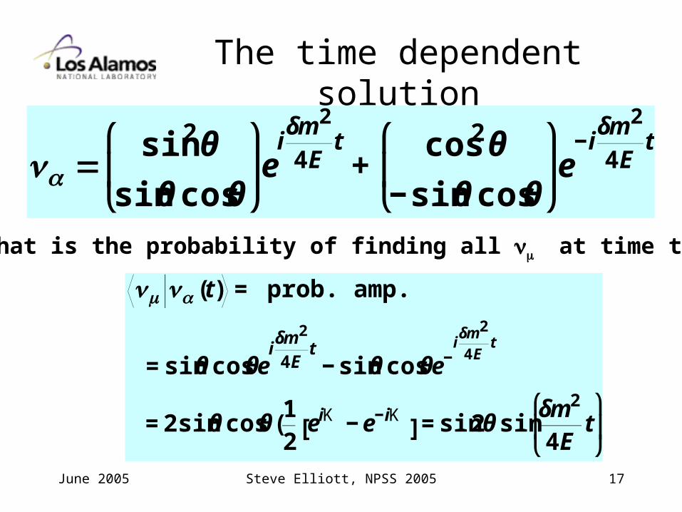
The time dependent solution

€

α =sin2 θ

sinθ cosθ

⎛

⎝ ⎜

⎞

⎠ ⎟e

iδm2

4Et+

cos2 θ

−sinθ cosθ

⎛

⎝ ⎜

⎞

⎠ ⎟e

−iδm2

4Et

What is the probability of finding all at time t?

€

α (t) = prob. amp.

= sinθ cosθeiδm2

4Et− sinθ cosθe−

iδm2

4Et

= 2sinθ cosθ (12

eiK − e−iK[ ] = sin2θ sin

δm2

4Et

⎛

⎝ ⎜

⎞

⎠ ⎟


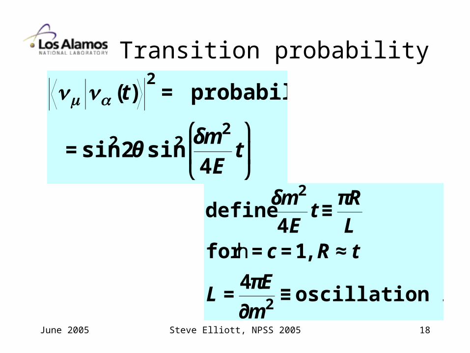
Transition probability

€

α (t)2

= probability

= sin2 2θ sin2 δm2

4Et

⎛

⎝ ⎜

⎞

⎠ ⎟

€

define δm2

4Et ≡

πRL

for h = c = 1, R ≈ t

L =4πE

∂m2 ≡ oscillation length


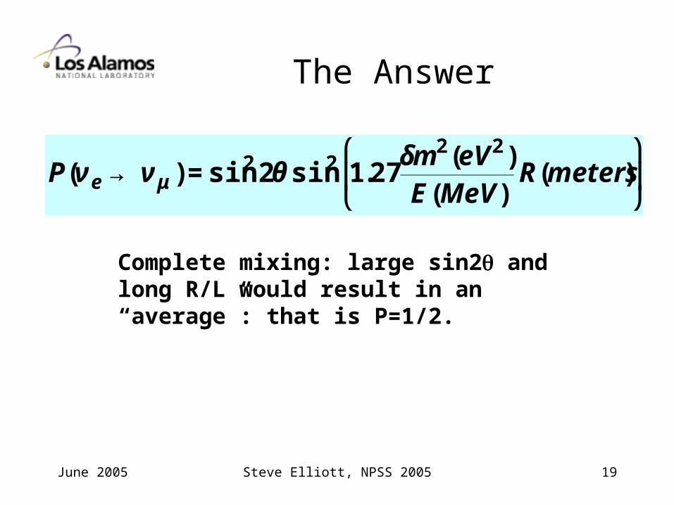
The Answer

€

P(ν e → ν μ ) = sin2 2θ sin2 1.27δm2 (eV2 )E(MeV)

R(meters) ⎛

⎝ ⎜

⎞

⎠ ⎟

Complete mixing: large sin2 and long R/L would result in an “average”: that is P=1/2.


What about MSW?

The Sun is mostly electrons (not muons).

e can forward scatter from electrons via the charged or neutral current.

can only forward scatter via the neutral current.

The e picks up an effective mass term, which acts on the weak eigenstates.


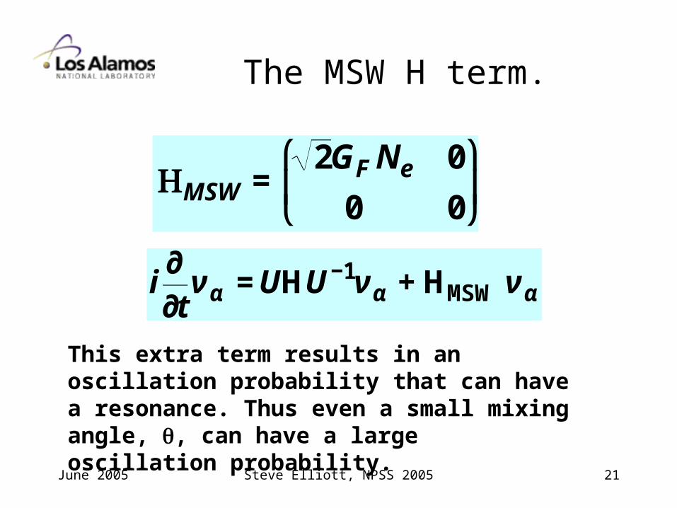
The MSW H term.

€

HMSW =2GFNe 0

0 0

⎛

⎝ ⎜

⎞

⎠ ⎟

€

i∂∂t

ν α = UHU−1ν α + HMSWν α

This extra term results in an oscillation probability that can have a resonance. Thus even a small mixing angle, , can have a large oscillation probability.


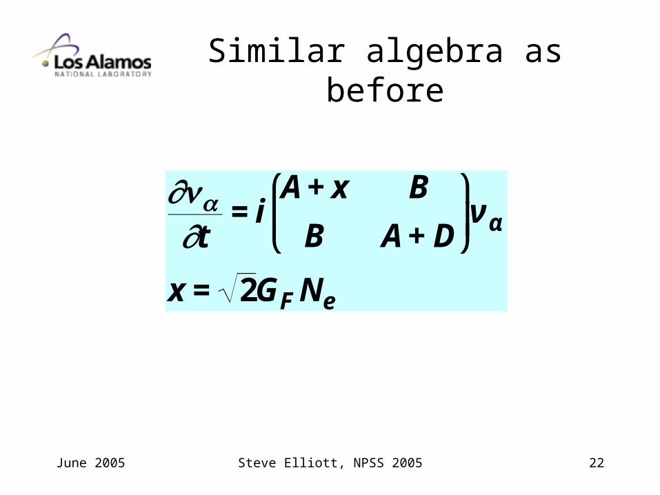
Similar algebra as before

€

∂α∂t

= iA+ x B

B A+ D

⎛

⎝ ⎜

⎞

⎠ ⎟ν α

x = 2GFNe


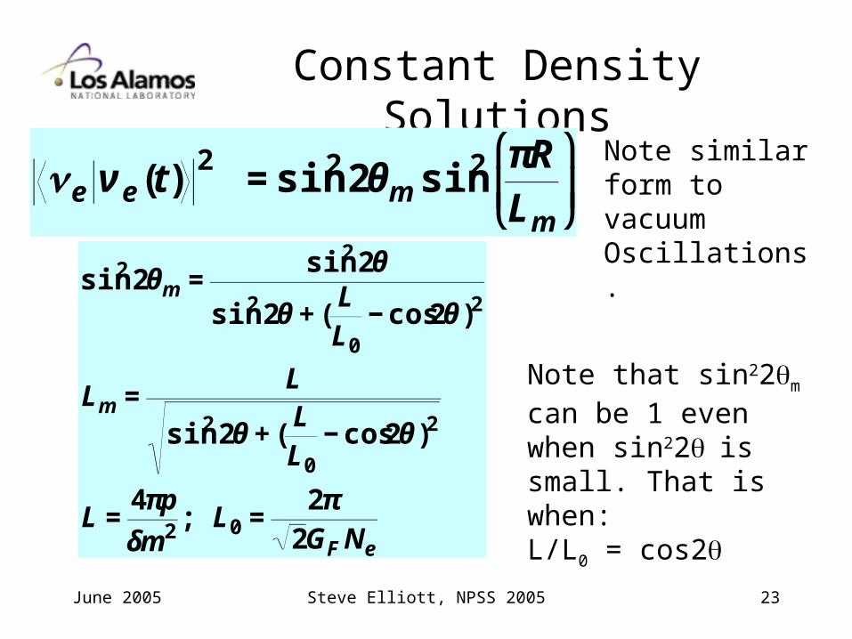
Constant Density Solutions

€

e ν e (t)2

= sin2 2θm sin2 πRLm

⎛

⎝ ⎜

⎞

⎠ ⎟

Note similar form to vacuumOscillations.

€

sin2 2θm =sin2 2θ

sin2 2θ + (LL0

− cos2θ )2

Lm =L

sin2 2θ + (LL0

− cos2θ )2

L =4πp

δm2 ; L0 =2π

2GFNe

Note that sin22m can be 1 even when sin22 is small. That is when:L/L0 = cos2


Variable Density

• Integrate over the changing density (such as in a star).


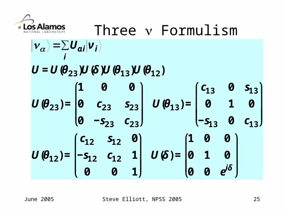
Three Formulism

€

α = Uαii

∑ ν i

U = U(θ23 )U(δ)U(θ13 )U(θ12 )

U(θ23 ) =

1 0 0

0 c23 s23

0 −s23 c23

⎛

⎝

⎜ ⎜ ⎜

⎞

⎠

⎟ ⎟ ⎟ U(θ13 ) =

c13 0 s13

0 1 0

−s13 0 c13

⎛

⎝

⎜ ⎜ ⎜

⎞

⎠

⎟ ⎟ ⎟

U(θ12 ) =

c12 s12 0

−s12 c12 1

0 0 1

⎛

⎝

⎜ ⎜ ⎜

⎞

⎠

⎟ ⎟ ⎟ U(δ) =

1 0 0

0 1 0

0 0 eiδ

⎛

⎝

⎜ ⎜ ⎜

⎞

⎠

⎟ ⎟ ⎟


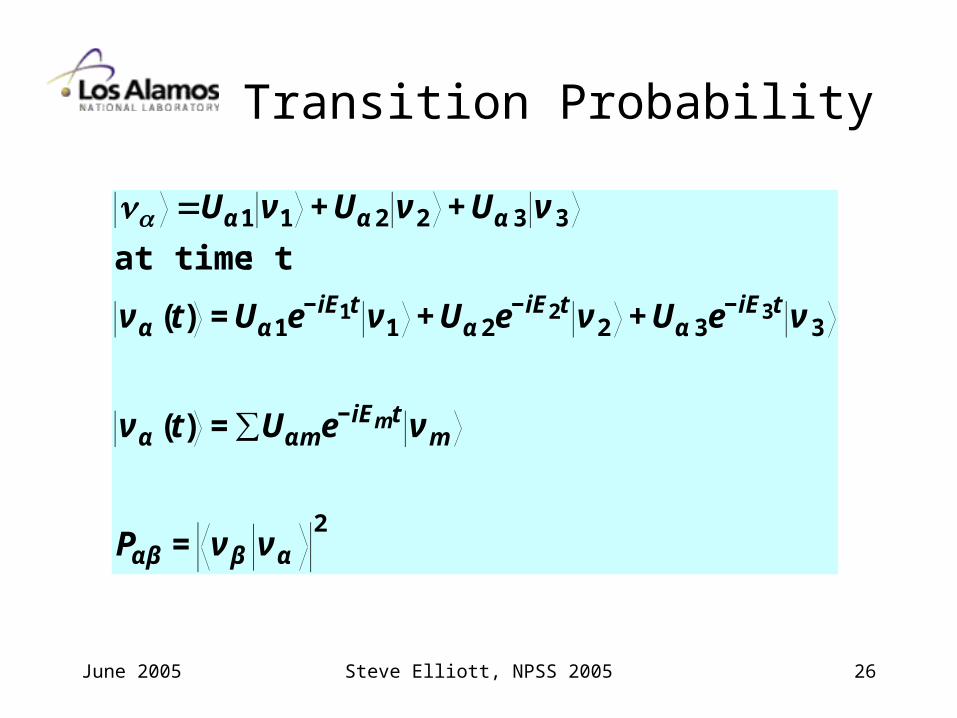
Transition Probability

€

α =Uα 1 ν 1 + Uα 2 ν 2 + Uα 3 ν 3

at time t :

ν α (t) = Uα 1e−iE1t ν 1 + Uα 2e−iE2t ν 2 + Uα 3e−iE3t ν 3

ν α (t) = Uαm∑ e−iEmt ν m

Pαβ = ν β ν α2


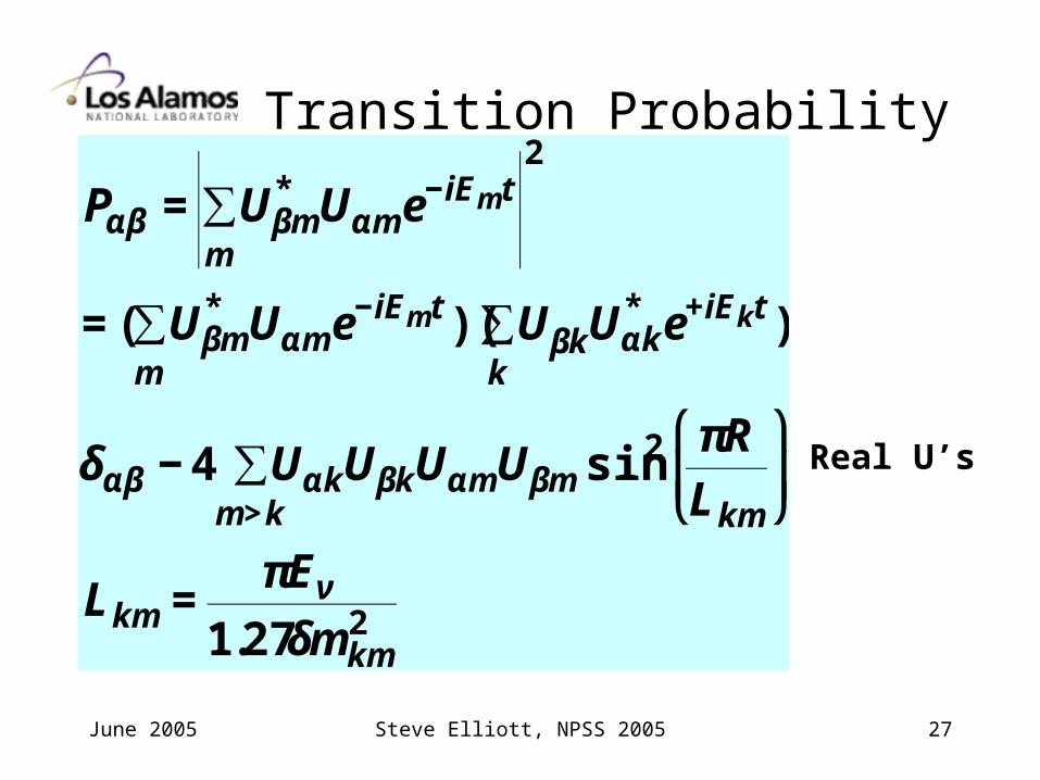
Transition Probability

€

Pαβ = Uβm* Uαme−iEmt

m∑

2

= ( Uβm* Uαme−iEmt

m∑ )( UβkUαk

* e+iEkt

k∑ )

δαβ − 4 UαkUβkUαmUβm sinm>k∑ 2 πR

Lkm

⎛

⎝ ⎜

⎞

⎠ ⎟

Lkm =πEν

1.27δmkm2

Real U’s


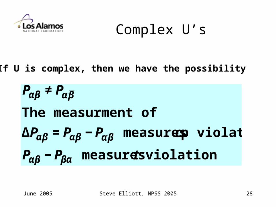
Complex U’s

If U is complex, then we have the possibility

€

Pαβ ≠ Pα β

The measurment of

ΔPαβ = Pαβ − Pα β measures cp violation

Pαβ − Pβα measures t violation


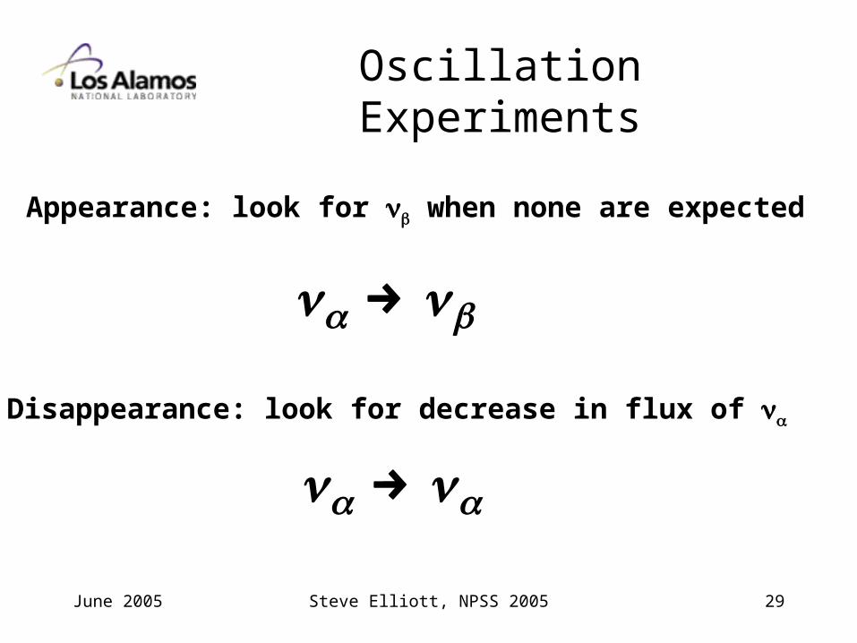
Oscillation Experiments

Appearance: look for when none are expected

Disappearance: look for decrease in flux of α

€

α →

€

α → α


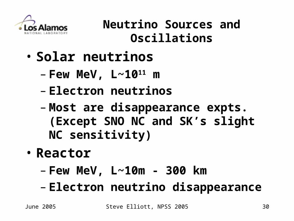
Neutrino Sources and Oscillations

• Solar neutrinos– Few MeV, L~1011 m– Electron neutrinos– Most are disappearance expts. (Except

SNO NC and SK’s slight NC sensitivity)

• Reactor– Few MeV, L~10m - 300 km– Electron neutrino disappearance


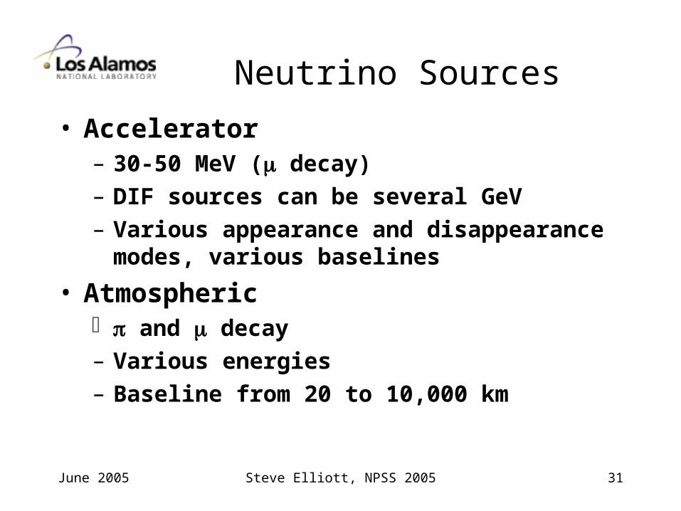
Neutrino Sources

• Accelerator– 30-50 MeV ( decay)– DIF sources can be several GeV– Various appearance and disappearance

modes, various baselines

• Atmospheric and decay– Various energies– Baseline from 20 to 10,000 km


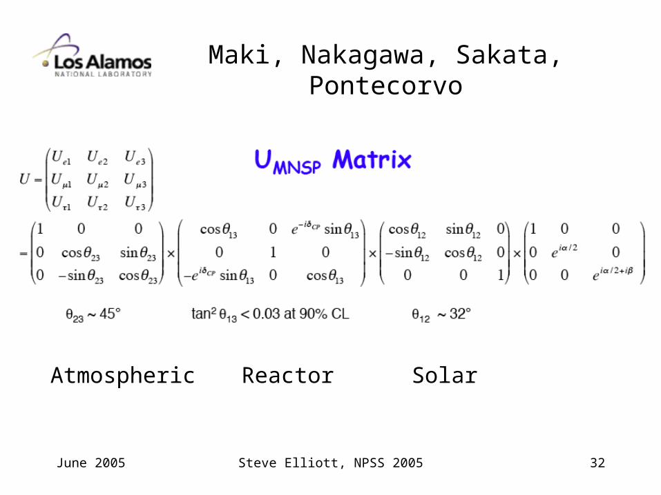
SolarReactorAtmospheric

Maki, Nakagawa, Sakata, Pontecorvo


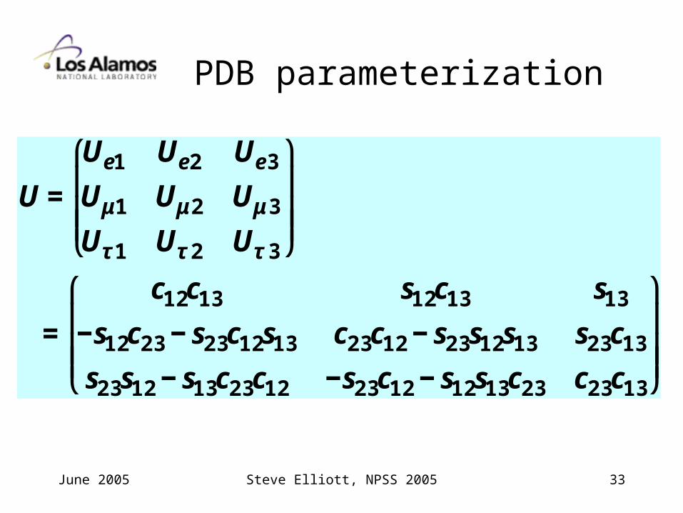
PDB parameterization

€

U =

Ue1 Ue2 Ue3

Uμ1 Uμ2 Uμ 3

Uτ 1 Uτ 2 Uτ 3

⎛

⎝

⎜ ⎜ ⎜

⎞

⎠

⎟ ⎟ ⎟

=

c12c13 s12c13 s13

−s12c23 − s23c12s13 c23c12 − s23s12s13 s23c13

s23s12 − s13c23c12 −s23c12 − s12s13c23 c23c13

⎛

⎝

⎜ ⎜ ⎜

⎞

⎠

⎟ ⎟ ⎟


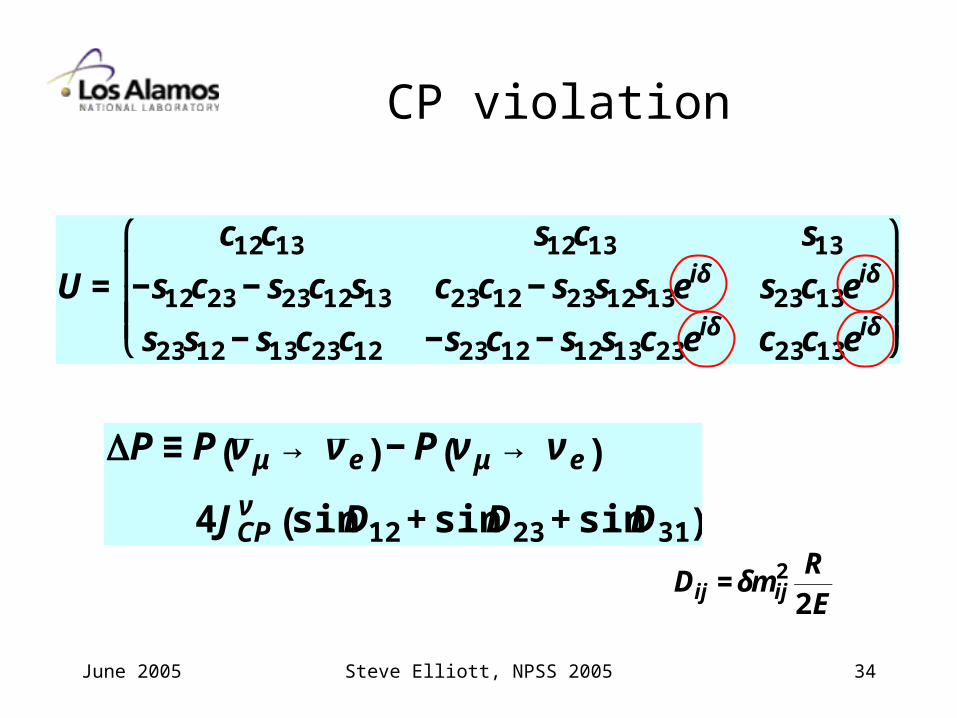
CP violation

€

U =

c12c13 s12c13 s13

−s12c23 − s23c12s13 c23c12 − s23s12s13eiδ s23c13eiδ

s23s12 − s13c23c12 −s23c12 − s12s13c23eiδ c23c13eiδ

⎛

⎝

⎜ ⎜ ⎜

⎞

⎠

⎟ ⎟ ⎟

€

ΔP ≡ P ν μ → ν e( ) − P ν μ → ν e( )

4JCPν sin D12 + sin D23 + sin D31( )

€

Dij = δmij2 R

2E


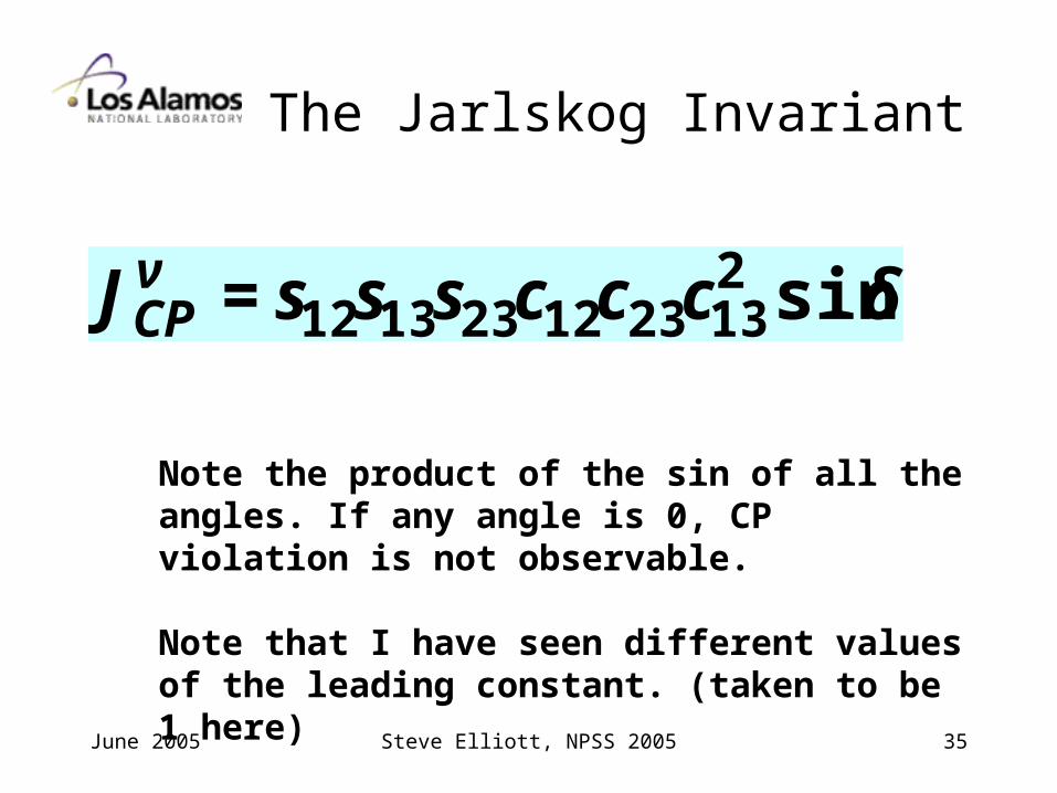
The Jarlskog Invariant

€

JCPν = s12s13s23c12c23c13

2 sinδ

Note the product of the sin of all the angles. If any angle is 0, CP violation is not observable.

Note that I have seen different values of the leading constant. (taken to be 1 here)


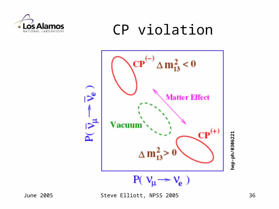
CP violation

he

p-p

h/0

30

62

21


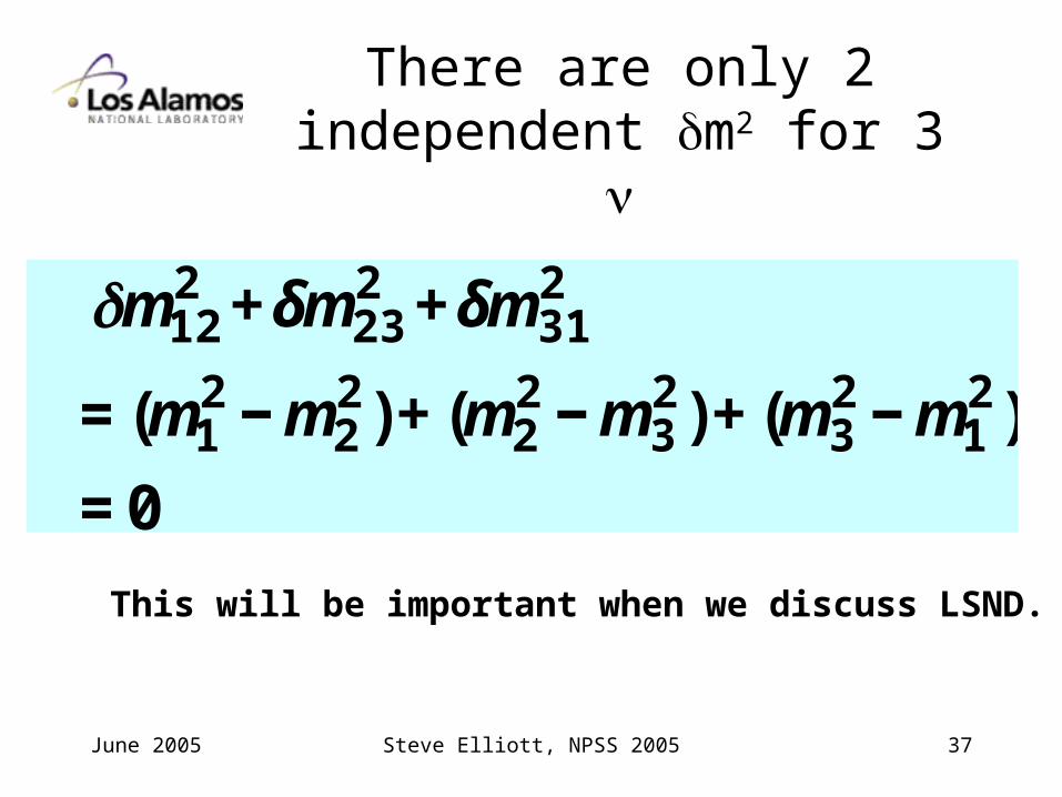
There are only 2 independent m2 for 3

€

m122 +δm23

2 +δm312

= (m12 − m2

2 )+ (m22 − m3

2 )+ (m32 − m1

2 )

= 0

This will be important when we discuss LSND.


Resources

• Steve Elliott - UW Phys 558 class notes

• Bahcall Book

• Many phenomenology papers

neutrino oscillations or how we know most of what we know

Documents

steve elliott

u slide

sin slide

formulism slide

vector slide

cos2 slide

solution of h slide

transition probability