neural networks with counter-propagation learning strategy used for modelling

E L S E V I E R Chemometrics and Intelligent Laboratory Systems 27 (1995) 175-187

Chemometrics and intelligent laboratory systems

Neural networks with counter-propagation learning strategy used for modelling

Jure Zupan a,. Marjana Novi~: a, Johann Gasteiger b a Laboratory of Chemometrics, National Institute of Chemistry, Hajdrihot~a 19, 61115 Ljubljana, Sloc,enia

b CCC, University ofErlangen, Niirnberg, Niigelsbacherstrasse 25, 91052 Erlangen, Germany

Received 18 November 1993; accepted 18 February 1994

Abstract

The neural networks employing the counter-propagation learning strategy are described and their use for making complex models and inverse models is explained. Two examples show how such modelling strategy can yield satisfactory results for the investigated systems. The first example describes building a model for quantitative prediction of the so-called 'colour change' factor. The second example shows the generation of the forward and inverse model for the control of a chemical process in a non-isothermic continuously stirred tank reactor (CSTR).

1. Introduct ion

Mode l l i ng of the complex mul t i -var ia te and mul t i - r e sponse systems in chemis t ry is a task of- ten employed in many b ranches of chemistry. In the last few years the use of ar t i f icial neura l ne tworks is becoming increas ingly intensive [1-5] in this f ield as well. In genera l , the mode l is a p r o c e d u r e y ie ld ing an n - response answer for each m-var ia te input. In the most of ten used polyno- mial mode l l ing the sought n - r e sponse vec tor Y is based on the funct ion F of m var iab les x i and p p a r a m e t e r s w k in the fol lowing way:

Y = ( Y l ,Y2 . . . . Y i , ' ' ' Yn)

= F ( X l , X z , . . . x j . . . . X m , W l , W 2 . . . . w k . . . . Wp)

(1)

* Corresponding author. Fax: (+38-61)263-061.

or

Y = { M } X (2)

where Y and X are mul t id imens iona l vectors , with c o m p o n e n t s Yi and x j, respect ively, and w k are p a r a m e t e r s de t e rmin ing the funct ion F . In Eq. (2), {M} is a complex non- l inea r o p e r a t o r in the form of one or more mat r ices c o m p o s e d of many p a r a m e t e r s Wlk. The above Eqs. (1) and (2) descr ibe the solut ion of the p r o b l e m via a system of n equa t ions which can be l inear or non- l inear , or via one or more n × m d imens iona l matr ix(ces) and vectors c o m p o s e d toge the r in var ious forms.

If the found (buil t or ob t a ined ) mode l describes the m e a s u r e m e n t space sat isfactori ly, the comple t e set of the response va lues within Y (n -d imens iona l r e sponse vec tor Y) can be calcu- l a ted for any m - d i m e n s i o n a l input X t aken f rom the m e a s u r e m e n t space covered by the model .

The eva lua t ion of the responses f rom the inputs is ca l led the ' f o rward so lu t ion ' of the p rob-

0169-7439/95/$09.50 © 1995 Elsevier Science B.V. All rights reserved SSDI 0169-7439(94)00016-C

176 J. Zupan et al. / Chemometrics and Intelligent Laboratory Systerns 27 (1995) 175-187

lem and the functions F or {M} are the forward model M. In many applications, however, even more desirable than the forward model M is its inverse - - the inverse model M-~ which allows to calculate X from Y.

From a mathematical point of view, it is considered that obtaining the inverse model from the forward model is a more difficult task than obtaining the forward model itself. Basically, this is due to the fact that the modelling function for setting up the forward model is known or at least can be guessed or approximated in advance while the inverse function is much harder to express analytically. Therefore, the methods that can pro- vide the inverse model with the same range of errors and with the same computational efforts as the forward model are extremely valuable and worthwhile to explore.

It is interesting to note that the counter-propagation neural networks (in contrast to the error back-propagation neural networks) offer the pos- sibility to obtain the inverse model simultaneously with the forward model in a very elegant and computationally efficient manner [5].

The main purpose of this paper is to show that the counter-propagation learning scheme within two-layer neural networks has the capability to build very reliable models from which the inverse models can be derived without any further calcu- lations.

2. About the supervised learning methods

No mat ter which method, be it the classical or neural network approach, is chosen for obtaining a complex multi-variate multi-response model, it always requires supervised learning. The name 'supervised' learning [6-8] defines a procedure in which during the training period the input and the requested output (response) values are known in advance. Both, the input and the desired target values, must be used (or ' input ' to the procedure) during the learning phase. Using the difference between the output predicted by the procedure called the 'model ' ( 'system') and the actual response (experimental values), the system is corrected in such a way that in the next run the

output will bet ter predict the correct answer. This means that for each step the performance of the system is improved compared to the previous one. The training or building of the model lasts until for all input vectors X the agreement between the model responses and actual desired targets are within the adequate tolerance limits or until the iteration quota or the number of learning attempts is exceeded.

Generally speaking, this procedure is used in all supervised learning methods, neural networks including. The way how the differences between the outputs and targets are used for the correction of the internal system's (model 's) parameters in order to improve its performance determines the learning strategy.

There are, however, some important advan- tages of neural networks over the classical ap- proaches. Most beneficial to the users are that no explicit knowledge in the form of functions for modelling is necessary, that the neural networks can handle continuous variables as well as those having discrete values, and that neural networks can easily model the inverse functions and therefore build inverse models.

According to most of the reviews on the use of neural networks in chemistry [1-5], the modelling problem was almost exclusively solved by the so- called 'error back-propagation' [9] learning strategy. There are many different chemical applications of this method in the literature and the reader is advised to consider one of the reviews on the subject [1-5]. The main disadvantage of the back-propagation approach is the fact that the weights in the trained neurons, representing the final synapse strengths, do not bear or have any specific meaning or relevance to the problem the neural network is supposed to solve.

In order to show how this deficiency can be solved even in the neural network approach, we shall introduce the counter-propagation learning strategy for building the models.

3. Counter-propagation learning strategy

Counter-propagation [10-12,5] is one of the less commonly used neural network learning

J. Zupan et al. /Chemornetrics and Intelligent Laboratory Systems 27 (1095) 175 187 177

strategies. Therefore , a description of the basic learning algorithm will be given here. Al though both supervised learning methods in neural networks have very similar names, namely error back-propagat ion learning [9,13] and counter- propagat ion learning, they are quite different when looking at the actual procedures for changing weights in neurons that form the neural network. However , they have some features in com- mon when looking at both methods from the organisational point of view.

First, they both require a set of ob jec t - t a rge t pairs (or i n p u t - o u t p u t pairs) of data for training and verification and second, the architecture of both neural networks is a multi-layer one. Er ror back-propagat ion feed-forward network can have two, three or even more layers, while counter- propagat ion network always has only two layers: the input and the output layer.

On the o ther hand, both methods differ con- siderably when looking at the connect ion of neurons between the layers. In the feed forward architecture all neurons in two adjacent layers are fully in terconnected, i.e., the signal f rom each neuron of the upper layer is connec ted to all neurons in the layer below. In the case of counter -propagat ion , the situation is quite differ-

ent. Here, each single neuron in the input layer is connected only to one neuron in the output layer.

The most significant distinction between both methods is in the way the target values are employed in the learning procedure . Actually, there are two separate differences in the entire procedure. The first difference is that in the counter- propagat ion strategy the target values are actually input to the network, i.c., the desired output is input to the selected neuron. In the error back- propagat ion network, however, only the difference between the actual output and the target is used for the correction. The second difference concerns the way of correct ion of the weights in neurons. In error back-propagat ion learning all weights in all neurons from all layers are corrected as soon as the input vector X produces an output Out different from the desired target Y. In the counter -propagat ion approach the weights in neurons belonging to the input layer are corrected (or better: adapted) according to the input vector X, while the weights in neurons belonging to the output layer are adapted according to the target vector Y. Additionally, in this strategy, the number of neurons in which the weights are corrected is permanent ly decreasing during the training to such an extent that at the closing

N i x Nj neurons Winning neuron

/} Weight levels Input X :il Test input 1 [] ,~, Kohonen layer [] 2 [] ) []

[] D - - - -

[] []

m [] []

/ ' Output layer Target input Y []

Prediction <3.

i i i i

i i i

/ ,̧̧ 5!

Training Testing

Fig. 1. Counter-propagation neural network architecture. The neurons are presented as vertical columns (dashed column) ordered in a N/× N i block. The weights in neurons in the input (Kohonen) and in the output layer are arranged in levels. There are as many weight levels as there are variables. In the training phase, the target values are input into the output layer (left), while during the testing and predictions the answers are taken out of the output layer (right).

178 J. Zupan et a l . / Chernometrics and Intelligent Laboratory Systems 27 (1995) 17.5-187

phase of learning the weights in one neuron only are corrected.

In short, the basic difference between the error back-propagation and the counter-propagation networks is that the former method calculates the answer, while the latter calculates the pointer to the location where the answer is stored: a counter-propagation network is thus a look-up table.

A counter-propagation network can best be visualised as two rectangular blocks composed of an equal number of neurons one above the other (Fig. 1). The upper block acts as the input (or Kohonen [14,15]) layer, while the second block in which the neurons have a different number of weights acts as the 'receiver' and the 'distributor' of the target information. The number of weights rn in neurons of the Kohonen layer is equal to the number of variables of the input vector X, while the number of weights n in the output layer neurons is equal to the number of target answers.

The counter-propagation learning strategy is very simple. One step in this procedure is composed of four acts:

1. Input of object X~ = ( X s l , X s 2 , . . . Xsi . . . . Xsm)

to the Kohonen layer and finding the neuron c (for central) in the Kohonen layer that has the weights w,~ (superscript K for Kohonen) most similar to the input variables (Eq. (4)).

2. Correcting all weights of the central neuron w~ and all weights wj~ in a certain neighbourhood of the neuron c in the Kohonen layer according to Eq. (5).

3. Using the position of neuron c as a 'pointer ' to the neuron in the output layer to which the target vector Ys (Ysl,Ys2 . . . . Ysi . . . . Ysn) should be input.

4. Correcting all weights of the central neuron %o (upper index o for output) and all weights w) °

in a certain neighbourhood in the output layer according to Eq. (5).

The same four acts are repeated for each object-target pair {X~,~} from the training set. Once all {X~,Y s} pairs of the training set are sent through the network one epoch of learning is accomplished. The learning procedure can be repeated either until the cumulative correction of weights in the last epoch does not exceed a

certain small threshold number or until the number of pre-defined learning epochs is accomplished.

Finding the position of the winning or central neuron c for each vector X input into the Koho- nen layer is achieved by comparing its components x i with all weights of all j neurons in the

a ( r 0 - r j )

,,ill[ Illl,, re

O O O O 0 0 0 0 0 0 0 0 O O O O 0 0 O O O O 0 0 o o r u u u o o o o o o o o o l o © U o o o o o o o 0 0 0 0 0 0 0 0 0

0 1 0 1 0 1 0 0 0 0 0 0 0 0 0 0 0 0 0 0 0 0 0 0 0 0 0 0 0 0 ~ 0 0 0 o o o o OlOlOlOlO o o o o o o o l o o o l o o o 0 0 0 0 0 0 0 0 0 0 0 OIQIOIO 0 0 0 0 0 O 0 0 1 0 1 0 0 0 0 0 0 0 0 0 0 1 0 0 0 0 0 0 0 0 0 0

0 0 0 0 0 0 0 0 0 0 0 0 O 0 0 0 0 0 0 0 O O 0 0

0 0 0 0 0 0 0 0 0 0 0 0 !ooo C O 0 I 0 0 0 i ooo 0 0 0 0 0 0 ,,_, 0 0 0 0 0 0 0 0 0 0 0 0 0 0

Fig. 2. Square neighbourhoods ('rings') around the central (most excited) neuron c are determined after each input. The number of concentric 'rings' where the neurons are corrected decreases during the training. Simultaneously with decreasing number of 'rings' where the correction is applied, the correction factor a(r~. - rg), for a given iteration step nt, is decreasing.

J. Zupan et al. / Chemometrics and Intelligent

network. The closest ma tch def ines the winning neu ron c:

The equa t ions for cor rec t ing the weights a re as follows:

wjK(new) = wjK(°Id) + ,7( n t ) a ( r c -- r j , n t )

X(Xsj--wjKi `°ld,) (4)

with j runn ing f rom 1 to m.

W/°(new) = Wj°(TM) + h ( n t ) a ( r c - r j , n t )

X ( Ysj- Wj O °̀,d)) (5)

with j runn ing f rom 1 to n. In the above equat ions , r / (n , ) is a funct ion

mono ton ica l ly dec reas ing be tween two p ro -de -

Laboratory Systems 27 (1995) 175-187 179

f ined values ama x and ami n with the increas ing n u m b e r of i t e ra t ion s teps n t. T h e n e i g h b o u r h o o d funct ion a ( r c - r j , n , ) def ines the pe r c e n t a ge of ac tual cor rec t ion (be tween 0 and 1) which should be app l i ed on weights of the neu ron j which is at the topologica l d i s tance r c - r ~ f rom the cen t ra l neu ron c (Fig. 2). The la rger the d i s tance r c - r~, the smal ler is the co r rec t ion of weights . A t the beg inn ing of the l ea rn ing process the ne ighbour - hood funct ion a ( r c - r~,n t) encompasse s the neurons and co r r e spond ing weights of the en t i re network, while dur ing the l ea rn ing process the n e i g h b o u r h o o d of neurons en t i t l ed to be cor- r ec ted is shr inking unti l , at the closing epoch, the cor rec t ion is app l i ed only to the weights in the cent ra l neuron . The p a r a m e t e r n t indica tes the funct ion 's shr inking charac te r .

It can be easily seen that bo th Eqs. (4) and (5) a re vir tual ly the same except tha t in the case of

17 t l 9 23 21 15 27 3

29 25

30

33 19 13

28 36 31 32 8 1

26 35

24 22 4

34

16 14 12 10 7 18

20 6 2 5

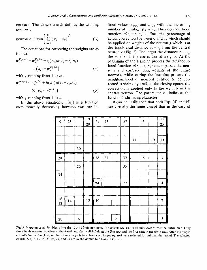
Fig. 3. Mapping of all 36 objects into the 12 × 12 Kohonen map. The objects are scattered quite evenly over the entire map. Only three fields contain two objects: the fourth and the twelfth field in the first row and the first field in the tenth row. After the map is cut into nine rectangles (bold tines), nine objects (one from each larger square) were selected for building the model. The selected objects 2, 4, 7, 13, 14, 23, 24, 27, and 28 are in the double line framed squares.

180 J. Zupan et aL / Chemometrics and Intelligent Laboratory Systems 27 (1995) 175-187

weights in the Kohonen neurons the correction is calculated using the components xsj of the input vector X s (Eq. (4)), while in the case of weights in the output neurons the corrections are calculated from the components Ysj of the corresponding target Y~ (Eq. (5)).

4. Example 1

The purpose of the following example is to describe how a simple model can solve a real world prediction problem and can additionally give some hints what the causes of the investigated behaviour of the relevant material are.

The goal was to find a model that would predict the development of an undesired effect, the so-called 'change of colour' in a certain product (paint) of one of Slovenian companies. In order to assure the quality of the product, the appearance of such an undesirable property should be predicted in advance, before the product leaves the company. The data available for each sample in question were concentrations of the eight most important additives and impurities (mainly oxides) that are regularly measured by the company's analytical laboratory.

The analytical work performed involves the analysis of eight oxides known to be present in the final product: A1203, P205, K20, F e O / Fe203, SiO2, Sb203, Nb205 and SO 3. Thus, each input vector X, describing the product s consists of eight components Xsj ( j = 1 . . . . . 8) - - concentrations of the mentioned oxides. The sequence order of oxides mentioned above does not reflect the actual order of concentration values used for input vector X s in the real application. The 'change of colour' value Ys for each product was measured relative to the other lot of the same sample not exposed to intensive treatment with moisture, higher temperature, and UV radiation. The 'change of colour' value of the sample X s is labelled as a single component response Y, (Y~I). The responses Ys are between 0 and 2, 0 being the best and 2 the worst value signalling the product that changes colour most. The value of 11, = 1 is the limiting value for the quality control check. The products having a 'change of colour' parameter higher than 1 are not acceptable and are either reprocessed or rejected.

Altogether complete analyses and measure- ments of 'colour change' of 36 products were available. From this number 9 pairs {X~,Y s} were selected to make the model and the remaining 27

12 x 12 neurons

Weight levels Xs

1 [AI203] [] 2 [P2 O5] [] 3 [K201 [] 4 [FeO]/[Fe203] [] 5 [SiO2] [] 6 [Sb203] [] " 7 [Nb205] [] 8 [so3] []

Ys Colourchange a <

)

Output layer

layer

Fig. 4. Architecture of the counter-propagation network for the first example. The Kohonen layer contains I44 neurons ordered in a 12 x 12 plane. Each neuron has eight weights: one weight for each input variable. The weights influenced by a given variable are regarded to form a level of weights. The neurons in the output layer have only one weight each, thus forming only one output level of weights.

Z Zupan et aL /Chemometrics and Intelligent Laboratory Systems 27 (1995) 175-187 181

pairs {X,,Y s} were r e t a ined for the test purpose . As desc r ibed e l sewhere [4,5], the division of the ent i re set of objects into a t ra in ing and a test set was m a d e using the K o h o n e n [5,14,15] m a p p i n g of all 36 p roduc t s on to a m a p of 12 x 12 neurons (Fig. 3).

By cut t ing the 12 × 12 K o h o n e n m a p having 144 neu rons into a reas consis t ing of 4 × 4 = 16 neu rons each, 9 a reas a r r a n g e d in a 3 × 3 grid are ob ta ined . F r o m each a rea only one object was se lected. The se lec ted objects are the p roduc t s Nos. 2, 4, 7, 13, 14, 23, 24, 27, and 28.

The n ine se lec ted products , each desc r ibed by the e igh t -d imens iona l vec tor Xs and the one-d i - mens iona l r e sponse gs, (s = 1 , . . . , 9 ) , were then employed in the c o u n t e r - p r o p a g a t i o n lea rn ing p r o c e d u r e using Eqs. (3)-(5) . The a rch i t ec tu re of the c o u n t e r - p r o p a g a t i o n ne twork for this example is shown in Fig. 4.

In this pa r t i cu l a r example we have used 300 epochs for the lea rn ing of 9 objects . The funct ion ~q(n t) mono ton ica l ly dec reas ing be tween 0.5 and 0.01 has the fol lowing form:

300 × 9 - n t r / ( n t ) = (0.5 - 0.01) 300 × 9 - 1 + 0.01 (6)

In our example , the funct ion a( r c - r j , n t) de-

12

( 8 Nj

1

1.4 +

Ni 1 2

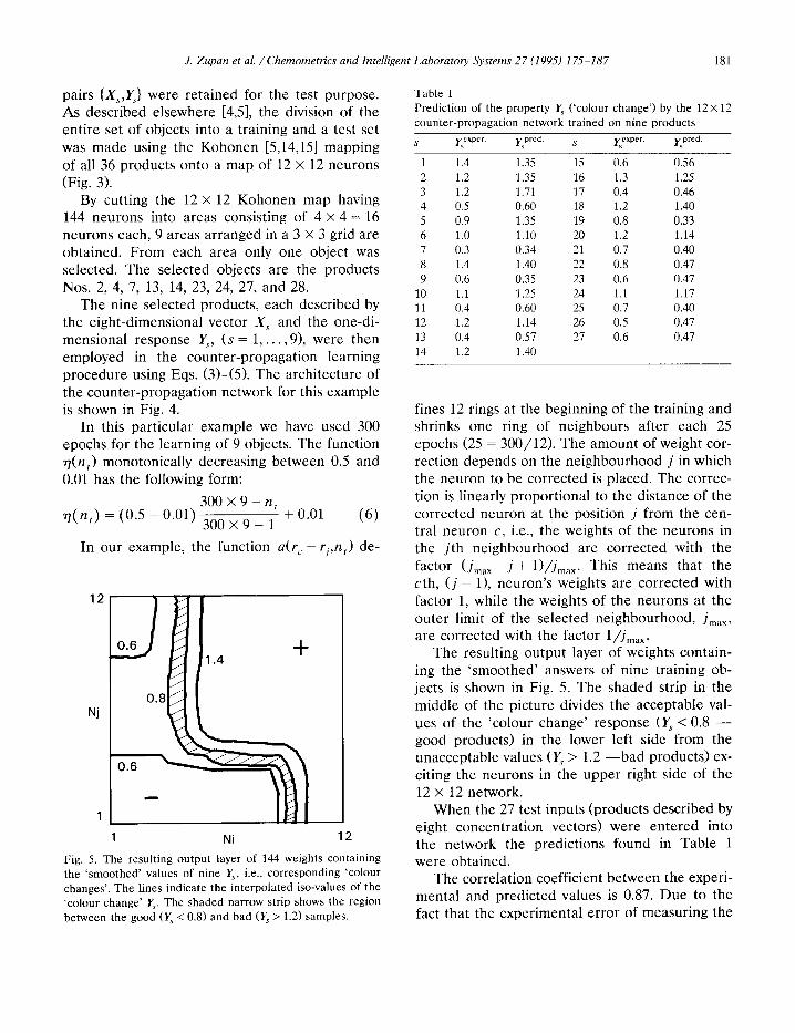
Fig. 5. The resulting output layer of 144 weights containing the 'smoothed' values of nine Ys, i.e., corresponding 'colour changes'. The lines indicate the interpolated iso-values of the 'colour change' Ys. The shaded narrow strip shows the region between the good (~ < 0.8) and bad (Ys > 1.2) samples.

Table 1 Prediction of the property Ys ('colour change') by the 12× 12 counter-propagation network trained on nine products s y oxp, yTroa s r~x~er, y Ored

1 1.4 1.35 15 0.6 0.56 2 1.2 1.35 16 1.3 1.25 3 1.2 1.71 17 0.4 0.46 4 0.5 0.60 18 1.2 1.40 5 0.9 1.35 19 0.8 0.33 6 1.0 1.10 20 1.2 1.14 7 0.3 0.34 21 0.7 0.40 8 1.4 1.40 22 0.8 0.47 9 0.6 0.35 23 0.6 0.47

10 1.1 1.25 24 1.1 1.17 11 0.4 0.60 25 0.7 0.40 12 1.2 1.14 26 0.5 0.47 13 0.4 0.57 27 0.6 0.47 14 1.2 1.40

fines 12 r ings at the beg inn ing of the t ra in ing and shrinks one r ing of ne ighbour s a f te r each 25 epochs (25 = 300/12) . The amoun t of weight correc t ion d e p e n d s on the n e i g h b o u r h o o d j" in which the neu ron to be co r r ec t ed is p laced . The correc- t ion is l inear ly p ropo r t i ona l to the d i s tance of the co r r ec t ed neu ron at the pos i t ion j f rom the cen- t ral neu ron c, i.e., the weights of the neurons in the j t h n e i g h b o u r h o o d are co r r ec t ed with the

fac tor ( J m a x - j + l) /Jma x. This means tha t the c th , ( j = 1), neu ron ' s weights a re co r r ec t ed with fac tor 1, while the weights of the neu rons at the ou te r l imit of the se lec ted ne ighbourhood , j . . . . a re co r rec t ed with the fac tor l /Jma x.

The resul t ing ou tpu t layer of weights conta in- ing the ' s m o o t h e d ' answers of nine t ra in ing objects is shown in Fig. 5. The s h a d e d str ip in the midd le of the p ic ture divides the accep tab le values of the ' co lour change ' r e sponse (Y, < 0.8 - - good p roduc t s ) in the lower left s ide f rom the una c c e p t a b l e values (¥s > 1.2 - - b a d p roduc t s ) ex- ci t ing the neu rons in the u p p e r r ight s ide of the 12 × 12 network.

W h e n the 27 test inputs (p roduc t s desc r ibed by e ight concen t ra t ion vectors) were e n t e r e d into the ne twork the p red ic t ions found in Tab le 1 were ob ta ined .

The cor re la t ion coeff ic ient be tw e e n the exper i - men ta l and p r e d i c t e d values is 0.87. D u e to the fact tha t the expe r imen ta l e r ro r of measu r ing the

182 J. Zupan et al. / Chemometrics and Intelligent Laboratory Systems 27 (1995) 175-187

'colour change' of the product is quite high, i.e., _+0.2 (more than 10%), the model predicts the quantitative values of Ys quite well.

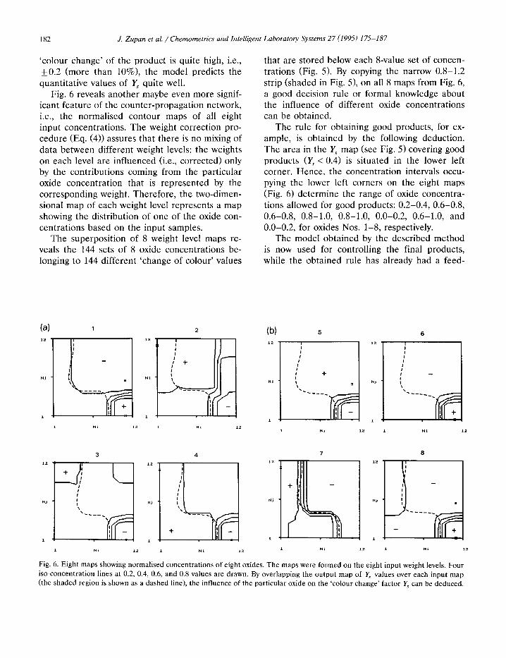
Fig. 6 reveals another maybe even more significant feature of the counter-propagation network, i.e., the normalised contour maps of all eight input concentrations. The weight correction procedure (Eq. (4)) assures that there is no mixing of data between different weight levels: the weights on each level are influenced (i.e., corrected) only by the contributions coming from the particular oxide concentration that is represented by the corresponding weight. Therefore, the two-dimensional map of each weight level represents a map showing the distribution of one of the oxide concentrations based on the input samples.

The superposition of 8 weight level maps reveals the 144 sets of 8 oxide concentrations belonging to 144 different 'change of colour' values

that are stored below each 8-value set of concentrations (Fig. 5). By copying the narrow 0.8-1.2 strip (shaded in Fig. 5), on all 8 maps from Fig. 6, a good decision rule or formal knowledge about the influence of different oxide concentrations can be obtained.

The rule for obtaining good products, for example, is obtained by the following deduction. The area in the Ys map (see Fig. 5) covering good products (Y~ < 0.4) is situated in the lower left corner. Hence, the concentration intervals occu- pying the lower left corners on the eight maps (Fig. 6) determine the range of oxide concentrations allowed for good products: 0.2-0.4, 0.6-0.8, 0.6-0.8, 0.8-1.0, 0.8-1.0, 0.0-0.2, 0.6-1.0, and 0.0-0.2 for oxides Nos. 1-8, respectively.

The model obtained by the described method is now used for controlling the final products, while the obtained rule has already had a feed-

(a) 1 2

N i 1 2

12

N j

2

I

/

I t

. . . . "I

t N i 12

(b) 1 2

1.

/ /

/ + I ,, [ ]

I

i !

/ _ .J I

1

3

- - - ~ , I

N j

1.

L_ i

1 N i 12

4

/

+ I -

1 H i 1 2

7

1 N i

8

e

1 N i

Fig. 6. Eight maps showing normalised concentrations of eight oxides. The maps were formed on the eight input weight levels. Four iso-concentration lines at 0.2, 0.4, 0.6, and 0.8 values are drawn. By overlapping the output map of Ys values over each input map (the shaded region is shown as a dashed line), the influence of the particular oxide on the 'colour change' factor Ys can be deduced.

J. Zupan et al. /Chemometrics and Intelligent Laboratory Systems 27 (1995) 175-187 183

back on those phases of the product ion process where the concent ra t ion of the most critical oxide impurities can be controlled.

5. E x a m p l e 2

The second example is in tended to show how from the direct model M produced by counter- propagat ion learning, the inverse model M-1 can be obtained. The actual example in this case represents the model for controll ing a chemical process in a non- isothermal continuously stirred tank reactor (CSTR). The problem how to obtain the direct and inverse models using the back- propagat ion learning strategy of feed-forward networks was already described by a group from the Depa r tmen t of Chemical Engineer ing at the University of Pennsylvania [16]. They produced the inverse model M - a using the same method and the same data as for the genera t ion of the direct error back-propagat ion strategy only by switching the inputs and outputs, i.e., having previous inputs as outputs and previous outputs as inputs. They showed that an error of about 4% in the predicted values is about the maximal precision that can be reached by the inverse model M-~ f rom the available data.

The use of the counter -propaga t ion learning strategy enables us to achieve two things: first, to genera te a direct model M yielding the prediction ability as good as that of a model obta ined by the error back-propagat ion method, and second, to genera te the inverse model M ~ simultaneously with the direct model having a predict ion er ror below 1%.

The state vector pc of a chemical process at t ime t is described by m variables

P ' = (Xl,X 2 . . . . x i . . . . Xm)t (7)

In order to predict how the process variable x i will vary with time, the values of this variable must be en tered to the learning process at the consecutive time events. In terms of the 'moving window' learning technique [4,5,16] the 'past hor izon ' of the training vector., i.e., the input vector X, must contain values of, let us say,

variable xi , spanning over 'previous ' events (Xi.t,

X i . , - l , Xi,, 2 . . . . ), while the ' fu ture horizon' , i.e., in the target vector Y, should contain the same variable x i recorded at the ' fu tu re ' time intervals, i.e., xi,t+l, xi.t+2, Yi,t+3, etc. The same is t rue for any other variable x r

The control over a process is exercised with two models: first, the model M for predict ion of critical parameters of the process for a few time intervals in the future and, second, the inverse model M 1 for predict ion of variable(s) that can be control led so that the system can be brought back to the normal condit ion if the predicted corrections are applied.

In this example a first-order reversible reaction A ~ R in the continuously stirred tank reactor (CSTR) is considered (Fig. 7).

The above reaction can be described by the following set of five non-l inear equat ions [16,17]:

d A t ( M i - A t ) - k l A t + k _ l R t

d t "r

d R t ( R i - R t ) - - - + k i A , - k 1R, d t "r -

dT, ( k l A , - k IR¢) _ _ _ - H ( T i - T , ) d t r

k 1 = B e - c / T ,

k _ 1 = D e - E l L (8)

d l ' - - ~

I A ., kl " R

A~, R t, T~

Fig. 7. Non-isothermal continuously stirred tank reactor (CSTR). A i and R i are the inlet concentrations of both reactants and T i is the corresponding temperature. At, Rt, and T t are the same variables at time t. The process can be manipulated using the inlet temperature ~ by specification of the 'should be' T m = T i value.

184 J. Zupan et al. / Chemometrics and Intelligent Laboratory Systems 27 (1995) 175-187

Table 2 Initial variable values and parameters used in the system of Eqs. (8)

A i = 1 mol/1 R i - 0 mol / l T /= 4 1 0 K B = 5 × 1 0 3 s l C = 5033 K D = l × 1 0 6 s t E = 7550 K H = 5 1 K / m o l r = 60 s

The inlet values A i and R i and the parameters in this system of Eqs. (8) have the values and units given in Table 2.

The data base of state variables At, R,, and T t, required for the training and testing of the model, was calculated for time intervals of 20 s by inserting the above parameters into the set of Eqs. (8) and integrating them. The data triplets covering a representative set of different cases can be obtained from Eqs. (8) by taking any given triplet of variables At, R, and T, and randomly changing the tempera ture T/ for the calculation of the new triplet A t + i , g t + 1 and 7",+ 1. Thus, the variable that is manipulated is the tempera ture T~. This randomly chosen temperature is considered as an additional variable T m (manipulated temperature) . The tempera ture T m specifies the input tempera ture ( T m = T,.) that the controller is imposing onto the system while T, is the temperature of the system if it is left to itself. The above procedure how to obtain the time sequence of the

triplets (A, , R t, T t) in equal time interval is explained in more detail in the literature [16,17].

The counter-propagation network selected for this example is made up of 5000 neurons spread out in two (50 x 50) layers.

The size of the network was selected on the assumption that a map of 2500 Kohonen neurons would offer enough place for the accommodation of 1000 process vectors each consisting of four variables: (A, , R,, T,, T m) without resulting in too many conflicts. At the same time, the 2500 neurons in the output layer assures the place for 2500 three-dimensional a n s w e r s ( A t + l , R t + l ,

Tt+~). The described counter-propagation network which has 5 0 × 5 0 × 4 + 5 0 × 5 0 × 3 = 35 000 weights is schematically shown in Fig. 8.

Selecting the central neuron c and the corrections of weights wj~ and wj ° in the Kohonen and in the output layer, respectively, was made using Eqs. (3)-(5) as described in the previous section. In the present counter-propagation training 1000 input vectors X = ( A , , R,, T,, T m) with 1000 targets Y= (A,+l , R t + l , Tt+ 1) were used in a 20 epoch (i.e., 20000 inputs) long learning. The learning rate rl(nt) for 20 epochs and 1000 training vectors was calculated similarly to Eq. (6):

, 7 ( n , ) = (0 .5 - 0 . 0 1 ) 20 x 1000 - n t

20 x 1000 - 1 - 0.01 (9)

50 x 50 neurons

Weight levels

1 At 2 Rt 3 Tt 4 Tm

Kohonenlayer Xs

[ ] -

r.3

D'<a

rn<:l rn.<~

A t+l Output layer a t+l t t+l

Fig. 8. The architecture of the counter-propagation network used for learning the forward model M of the CSTR problem. The input layer has four levels of weights (for accepting the variables At, Rt, To, T m) and the output layer has three levels of weights for storing the three output variables (A t+ l , Rt+l, Tt+i).

Z Zupan et al. / Chemometrics and Intelligent Laboratory Systems 27 (1995) 175-187 185

Table 3 The recall and the prediction ability of the counter-propagation network

Variable Recall Prediction O" O" m e a n O" O" m e a n

A 0.004 1.2×10 .4 0 . 0 0 5 1.6×10 4 R 0.004 1.2×10 4 0 . 0 0 5 1.6×10 -4 T (K) 0.86 0.027 1.03 0.032

Af ter the stabilisation of the counter -propagation network is achieved (the training is com- pleted), the retrieval of predicted process vectors is straightforward. For each input query X (At , Rt, Tt, T TM) the neuron in the Kohonen network having weights wj~ most similar to the input variables x i (x I = A t , x 2 =R~, x 3 = Tt, x 4 = T m) is selected (Eq. (3)) as the 'winner ' c. Its position c is t ransmit ted to the output layer in which the weights w~ ° of the neuron at the specified position c contain the answer Y (At+a, Rt+l , Tt+l), i.e., the process variables at time t + 1.

The recall ability, i.e., the test for the retrieval of the answers for vectors X~ used in the training, was checked first. Later, the predict ion ability was tested with the set of another thousand process vectors X, not used in the training. The predict ion ability for all three process variables is given in Table 3.

Let us re turn to the archi tecture of the counter -propagat ion network for this study shown in Fig. 8. All seven weight levels are exactly o f the same size and stacked one above the other. The order in which they are ar ranged is arbitrary. The sequence that the upper four levels are used for input of variables at time t (A , , R, , 7",, T m) and that the lower three levels are used for the output of the variables at time t + 1, ( A t + l , R~+l, T~+ 1) is only the reflection of the sequence in which the process data are stored in the computer . What really matters is that the same variable (be it the input or the output variable) is always input to the same level of weights.

The fact that the position of weight levels does not mat ter at all offers an attractive idea o f rearranging them. If the weight levels are rearranged in a different order, a new network is obtained (Fig. 9).

The new ar rangement of the weight levels is chosen on purpose: the levels are now divided into two new groups: the upper group (the Koho- nen or input layer) consisting of six weight levels and the lower group (the output layer) consisting of only one level. This rear ranged stack of the weight levels can be regarded as a new counter- propagat ion neural network. Actually, however, the weights did not change at all - - what is different is only the order of levels. This means

50 x 50 neurons

Weight levels Xs

1 A t [] 2 Rt [] 3 Tt [] 4 Tt+ l [] 5 A t+l [] 6 R t+l []

T m D . , ~

/ ~ / , i

E> " .... = . E> E> E> .i ........ . ,

i i J i

i I i

S / i.- ..... ! , d

Kohonen layer

Output layer

Fig. 9. Rearrangement of seven weight levels of the forward model. The new network has six levels of weights in the input layer (At, Rt, Tt, At+l, R~+z, Tt+ ~) and only one level of weights in the output layer (Tin).

186 J. Zupan et al. /Chemometrics and Intelligent Laboratory Systems 27 (1995) 175-187

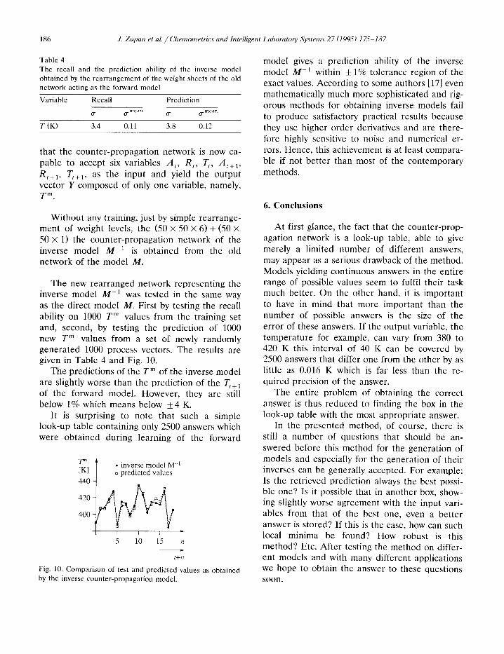
Table 4 The recall and the prediction ability of the inverse model obtained by the rear rangement of the weight sheets of the old network acting as the forward model

Variable Recall Prediction

O" O m e a n O" O " m e a n

T (K) 3.4 0.11 3.8 0.12

that the counter-propagation network is now ca- pable to accept six variables A t, Rt , T t, At+ ~,

Rt+ 1, Tt+~, as the input and yield the output vector Y composed of only one variable, namely, T m"

Without any training, just by simple rearrangement of weight levels, the (50 × 50 × 6) + (50 × 50 × 1) the counter-propagation network of the inverse model M -1 is obtained from the old network of the model M.

The new rearranged network representing the inverse model M-1 was tested in the same way as the direct model M. First by testing the recall ability on 1000 T m values from the training set and, second, by testing the prediction of 1000 new T m values from a set of newly randomly generated 1000 process vectors. The results are given in Table 4 and Fig. 10.

The predictions of the T m of the inverse model are slightly worse than the prediction of the T t+j of the forward model. However, they are still below 1% which means below _+4 K.

It is surprising to note that such a simple look-up table containing only 2500 answers which were obtained during learning of the forward

T'n • reverse model M -I [K] o predicted values 440 -

420-

400 -

I I I i ,

5 10 15 n

t + ~ l

Fig. 10. Comparison of test and predicted values as obtained by the inverse counter-propagation model.

model gives a prediction ability of the inverse model M - ~ within + 1% tolerance region of the exact values. According to some authors [17] even mathematically much more sophisticated and rig- orous methods for obtaining inverse models fail to produce satisfactory practical results because they use higher order derivatives and are therefore highly sensitive to noise and numerical errors. Hence, this achievement is at least compara- ble if not better than most of the contemporary methods.

6. Conclusions

At first glance, the fact that the counter-propagation network is a look-up table, able to give merely a limited number of different answers, may appear as a serious drawback of the method. Models yielding continuous answers in the entire range of possible values seem to fulfil their task much better. On the other hand, it is important to have in mind that more important than the number of possible answers is the size of the error of these answers. If the output variable, the temperature for example, can vary from 380 to 420 K this interval of 40 K can be covered by 2500 answers that differ one from the other by as little as 0.016 K which is far less than the required precision of the answer.

The entire problem of obtaining the correct answer is thus reduced to finding the box in the look-up table with the most appropriate answer.

In the presented method, of course, there is still a number of questions that should be an- swered before this method for the generation of models and especially for the generation of their inverses can be generally accepted. For example: Is the retrieved prediction always the best possible one? Is it possible that in another box, showing slightly worse agreement with the input variables from that of the best one, even a better answer is stored? If this is the case, how can such local minima be found? How robust is this method? Etc. After testing the method on different models and with many different applications we hope to obtain the answer to these questions s o o n .

J. Zupan et al. / Chemometrics and Intelligent Laboratory Systems 27 (1995) 175 187 187

Acknowledgement

The authors are highly indebted to the Min- istry of Science and Technology of Slovenia and to the Bundesminister fiir Forschung und Tech- nologie of the Federal Republic of Germany for financial support of this work.

Thanks are due to Ms. Nineta Majcen, M.Sc. and Ms. Karmen Rajer-Kandu5 from the Quality Assurance Department of the Cinkarna Co., Celje, Slovenia, for providing us with the analytical data used in the first example.

References

[1] J. Zupan and J. Gasteiger, Neural networks: a new method for solving chemical problems or just a passing phase? (a Review), Analytica Chimica Acta, 248 (19911 1-30.

[2] J. Gasteiger and J. Zupan, Neuronale Netze in der Chemie, Angewandte Chemie, 105 (1993) 510-536; Neu- ral networks in chemistry, Angewandte Chemie Interna- tional Edition in English, 32 (1993) 503-527.

[3] G. Kateman, Neural networks in analytical chemistry, Chemometrics and Intelligent Laboratory Systems, 19 (1993) 135-142.

[4] P. de B. Harrington, Minimal neural networks: differenti- ation of classification entropy, Chemornetrics and Intelli- gent Laboratory Systems, 19 (1993) 142-154.

[5] J. Zupan and J. Gasteiger, Neural Networks for Chemists: An Introduction, VCH, Weinheim, 1993.

[6] D.L. Massart, B.G.M. Vandeginste. S.N. Deming, Y. Michotte and L. Kaufmann, Chemometrics: a Textbook, Elsevier, Amsterdam, 1988.

[7] K. Varmuza, Pattern Recognition in Chemisto,, Springer Verlag, Berlin, I980.

[8] J. Zupan, Algorithms for Chemists, Wiley, Chichester, 1989.

[9] D.E. Rumelhart, G.E. Hinton and R.J. Williams, Learn- ing internal representations by error back-propagation, in D.E. Rumelhart and J.L. McClelland (Editors), Dis- tributed Parallel Processing: Explorations in the Microstrue- tures of Cognition, Vol. 1, MIT, Cambridge, MA, 1986, pp. 318-362.

[1(1] R. Hecht-Nielsen, Counterpropagation networks, Ap- plied Optics, 26 (1987) 4979-84.

[11] D.G. Stork, Counterpropagation networks: adaptive hier- archical networks for near optimal mappings, Synapse Connection, 1(2) (19881 9-17.

[12] J. Dayhoff, Neural Network Arehitectures, An Introduc- tion, Van Nostrand Reinhold, New York, 19911, chap. 10.

[13] R.P. Lipmann, An introduction to computing with neural nets, IEEE ASSP Magazine, April (1987) 155-162.

[14] T. Kohonen, Se!f-Organisation and Associatice Mernory, Springer Verlag, Berlin, 3rd edn., 1989.

[15] T. Kohonen, An introduction to neural computing, Neu- ral Networks, 1 (1988) 3 16.

[16] D.C. Psichogios and L.H. Ungar, Direct and indirect model based control using artificial neural networks, Industrial and Engineering Chemistry Research, 30 (1991) 2564-2573,

[17] C.E. Economu and M. Morari, Internal model control. 5. Extension to nonlinear systems, Industrial and Engineer- ing Chemistry Process Design and Del,elopment, 25 (1986) 403-411.

neural networks with counter-propagation learning strategy used for modelling

Documents