neural networks tutorial – a pathway to deep...
TRANSCRIPT

4/10/2017 Neural Networks Tutorial A Pathway to Deep Learning Adventures in Machine Learning
http://adventuresinmachinelearning.com/neuralnetworkstutorial/ 1/16
Neural Networks Tutorial – A Pathway to Deep LearningMarch 18, 2017 Andy
Chances are, if you are searching for a tutorial on artificial neural networks (ANN) you already have some idea of what they are, and what they are capable of doing. But didyou know that neural networks are the foundation of the new and exciting field of deep learning? Deep learning is the field of machine learning that is making many stateoftheart advancements, from beating players at Go and Poker, to speeding up drug discovery and assisting selfdriving cars. If these types of cutting edge applicationsexcite you like they excite me, then you will be interesting in learning as much as you can about deep learning. However, that requires you to know quite a bit abouthow neural networks work. This tutorial article is designed to help you get up to speed in neural networks as quickly as possible.
In this tutorial I’ll be presenting some concepts, code and maths that will enable you to build and understand a simple neural network. Some tutorials focus only on the codeand skip the maths – but this impedes understanding. I’ll take things as slowly as possible, but it might help to brush up on your matrices and differentiation if you need to.The code will be in Python, so it will be beneficial if you have a basic understanding of how Python works. You’ll pretty much get away with knowing about Python functions,loops and the basics of the numpy library. By the end of this neural networks tutorial you’ll be able to build an ANN in Python that will correctly classify handwritten digits inimages with a fair degree of accuracy.
Once you’re done with this tutorial, you can dive a little deeper with the following posts:
Improve your neural networks – Part 1 [TIPS AND TRICKS]Stochastic Gradient Descent – Minibatch and more
All of the relevant code in this tutorial can be found here.
Here’s an outline of the tutorial, with links, so you can easily navigate to the parts you want:
1 What are artificial neural networks?2 The structure of an ANN2.1 The artificial neuron2.2 Nodes2.3 The bias2.4 Putting together the structure2.5 The notation3 The feedforward pass3.1 A feedforward example3.2 Our first attempt at a feedforward function3.3 A more efficient implementation3.4 Vectorisation in neural networks3.5 Matrix multiplication4 Gradient descent and optimisation4.1 A simple example in code4.2 The cost function4.3 Gradient descent in neural networks4.4 A two dimensional gradient descent example4.5 Backpropagation in depth4.6 Propagating into the hidden layers4.7 Vectorisation of backpropagation4.8 Implementing the gradient descent step4.9 The final gradient descent algorithm5 Implementing the neural network in Python5.1 Scaling data5.2 Creating test and training datasets5.3 Setting up the output layer5.4 Creating the neural network5.5 Assessing the accuracy of the trained model
1 What are artificial neural networks?Artificial neural networks (ANNs) are software implementations of the neuronal structure of our brains. We don’t need to talk about the complex biology of our brainstructures, but suffice to say, the brain contains neurons which are kind of like organic switches. These can change their output state depending on the strength of theirelectrical or chemical input. The neural network in a person’s brain is a hugely interconnected network of neurons, where the output of any given neuron may be the input tothousands of other neurons. Learning occurs by repeatedly activating certain neural connections over others, and this reinforces those connections. This makes them morelikely to produce a desired outcome given a specified input. This learning involves feedback – when the desired outcome occurs, the neural connections causing thatoutcome become strengthened.
Artificial neural networks attempt to simplify and mimic this brain behaviour. They can be trained in a supervised or unsupervised manner. In a supervised ANN, the networkis trained by providing matched input and output data samples, with the intention of getting the ANN to provide a desired output for a given input. An example is an emailspam filter – the input training data could be the count of various words in the body of the email, and the output training data would be a classification of whether the email
4/10/2017 Neural Networks Tutorial A Pathway to Deep Learning Adventures in Machine Learning
http://adventuresinmachinelearning.com/neuralnetworkstutorial/ 2/16
was truly spam or not. If many examples of emails are passed through the neural network this allows the network to learn what input data makes it likely that an email isspam or not. This learning takes place be adjusting the weights of the ANN connections, but this will be discussed further in the next section.
Unsupervised learning in an ANN is an attempt to get the ANN to “understand” the structure of the provided input data “on its own”. This type of ANN will not be discussed inthis post.
2 The structure of an ANN
2.1 The artificial neuron
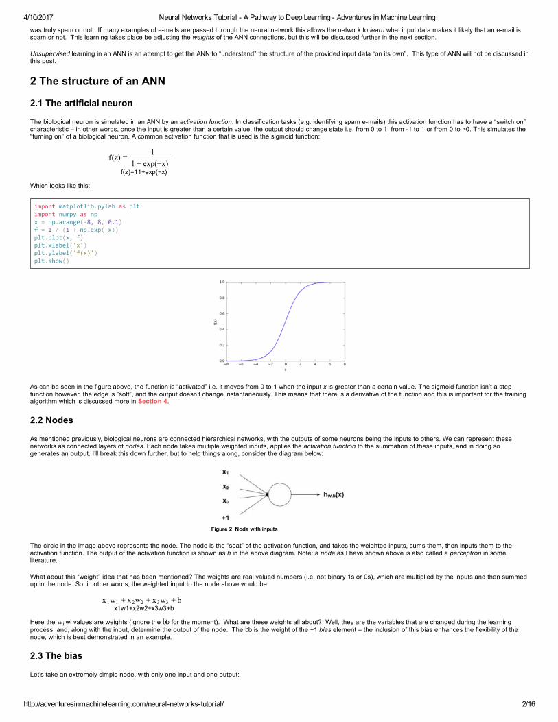
The biological neuron is simulated in an ANN by an activation function. In classification tasks (e.g. identifying spam emails) this activation function has to have a “switch on”characteristic – in other words, once the input is greater than a certain value, the output should change state i.e. from 0 to 1, from 1 to 1 or from 0 to >0. This simulates the“turning on” of a biological neuron. A common activation function that is used is the sigmoid function:
Which looks like this:
import matplotlib.pylab as plt import numpy as np x = np.arange(‐8, 8, 0.1) f = 1 / (1 + np.exp(‐x)) plt.plot(x, f) plt.xlabel('x') plt.ylabel('f(x)') plt.show()
As can be seen in the figure above, the function is “activated” i.e. it moves from 0 to 1 when the input x is greater than a certain value. The sigmoid function isn’t a stepfunction however, the edge is “soft”, and the output doesn’t change instantaneously. This means that there is a derivative of the function and this is important for the trainingalgorithm which is discussed more in Section 4.
2.2 Nodes
As mentioned previously, biological neurons are connected hierarchical networks, with the outputs of some neurons being the inputs to others. We can represent thesenetworks as connected layers of nodes. Each node takes multiple weighted inputs, applies the activation function to the summation of these inputs, and in doing sogenerates an output. I’ll break this down further, but to help things along, consider the diagram below:
Figure 2. Node with inputs
The circle in the image above represents the node. The node is the “seat” of the activation function, and takes the weighted inputs, sums them, then inputs them to theactivation function. The output of the activation function is shown as h in the above diagram. Note: a node as I have shown above is also called a perceptron in someliterature.
What about this “weight” idea that has been mentioned? The weights are real valued numbers (i.e. not binary 1s or 0s), which are multiplied by the inputs and then summedup in the node. So, in other words, the weighted input to the node above would be:
Here the values are weights (ignore the for the moment). What are these weights all about? Well, they are the variables that are changed during the learningprocess, and, along with the input, determine the output of the node. The is the weight of the +1 bias element – the inclusion of this bias enhances the flexibility of thenode, which is best demonstrated in an example.
2.3 The bias
Let’s take an extremely simple node, with only one input and one output:
f(z) =1
1 + exp(−x)f(z)=11+exp(−x)
+ + + bx1w1 x2w2 x3w3x1w1+x2w2+x3w3+b
wiwi bbbb

4/10/2017 Neural Networks Tutorial A Pathway to Deep Learning Adventures in Machine Learning
http://adventuresinmachinelearning.com/neuralnetworkstutorial/ 3/16
Figure 2. Simple node
The input to the activation function of the node in this case is simply . What does changing do in this simple network?
w1 = 0.5 w2 = 1.0 w3 = 2.0 l1 = 'w = 0.5' l2 = 'w = 1.0' l3 = 'w = 2.0' for w, l in [(w1, l1), (w2, l2), (w3, l3)]: f = 1 / (1 + np.exp(‐x*w)) plt.plot(x, f, label=l) plt.xlabel('x') plt.ylabel('h_w(x)') plt.legend(loc=2) plt.show()
Figure 4. Effect of adjusting weights
Here we can see that changing the weight changes the slope of the output of the sigmoid activation function, which is obviously useful if we want to model different strengthsof relationships between the input and output variables. However, what if we only want the output to change when x is greater than 1? This is where the bias comes in –let’s consider the same network with a bias input:
Figure 5. Effect of bias
w = 5.0 b1 = ‐8.0 b2 = 0.0 b3 = 8.0 l1 = 'b = ‐8.0' l2 = 'b = 0.0' l3 = 'b = 8.0' for b, l in [(b1, l1), (b2, l2), (b3, l3)]: f = 1 / (1 + np.exp(‐(x*w+b))) plt.plot(x, f, label=l) plt.xlabel('x') plt.ylabel('h_wb(x)') plt.legend(loc=2) plt.show()
Figure 6. Effect of bias adjusments
In this case, the has been increased to simulate a more defined “turn on” function. As you can see, by varying the bias “weight” , you can change when the nodeactivates. Therefore, by adding a bias term, you can make the node simulate a generic if function, i.e. if (x > z) then 1 else 0. Without a bias term, you are unable to varythe z in that if statement, it will be always stuck around 0. This is obviously very useful if you are trying to simulate conditional relationships.
x1w1x1w1 w1w1
w1w1 bb

4/10/2017 Neural Networks Tutorial A Pathway to Deep Learning Adventures in Machine Learning
http://adventuresinmachinelearning.com/neuralnetworkstutorial/ 4/16
2.4 Putting together the structure
Hopefully the previous explanations have given you a good overview of how a given node/neuron/perceptron in a neural network operates. However, as you are probablyaware, there are many such interconnected nodes in a fully fledged neural network. These structures can come in a myriad of different forms, but the most common simpleneural network structure consists of an input layer, a hidden layer and an output layer. An example of such a structure can be seen below:
Figure 10. Three layer neural network (again)
The three layers of the network can be seen in the above figure – Layer 1 represents the input layer, where the external input data enters the network. Layer 2 is calledthe hidden layer as this layer is not part of the input or output. Note: neural networks can have many hidden layers, but in this case for simplicity I have just included one.Finally, Layer 3 is the output layer. You can observe the many connections between the layers, in particular between Layer 1 (L1) and Layer 2 (L2). As can be seen, eachnode in L1 has a connection to all the nodes in L2. Likewise for the nodes in L2 to the single output node L3. Each of these connections will have an associated weight.
2.5 The notation
The maths below requires some fairly precise notation so that we know what we are talking about. The notation I am using here is similar to that used in the Stanford deeplearning tutorial. In the upcoming equations, each of these weights are identified with the following notation: . refers to the node number of the connection inlayer and refers to the node number of the connection in layer . Take special note of this order. So, for the connection between node 1 in layer 1 and node 2 inlayer 2, the weight notation would be . This notation may seem a bit odd, as you would expect the *i* and *j* to refer the node numbers in layers and
respectively (i.e. in the direction of input to output), rather than the opposite. However, this notation makes more sense when you add the bias.
As you can observe in the figure above – the (+1) bias is connected to each of the nodes in the subsequent layer. So the bias in layer 1 is connected to the all the nodes inlayer two. Because the bias is not a true node with an activation function, it has no inputs (it always outputs the value +1). The notation of the bias weight is , where*i* is the node number in the layer – the same as used for the normal weight notation . So, the weight on the connection between the bias in layer 1and the second node in layer 2 is given by .
Remember, these values – and – all need to be calculated in the training phase of the ANN.
Finally, the node output notation is , where denotes the node number in layer of the network. As can be observed in the three layer network above, the outputof node 2 in layer 2 has the notation of .
Now that we have the notation all sorted out, it is now time to look at how you calculate the output of the network when the input and the weights are known. The process ofcalculating the output of the neural network given these values is called the feedforward pass or process.
3 The feedforward passTo demonstrate how to calculate the output from the input in neural networks, let’s start with the specific case of the three layer neural network that was presented above.Below it is presented in equation form, then it will be demonstrated with a concrete example and some Python code:
In the equation above refers to the node activation function, in this case the sigmoid function. The first line, is the output of the first node in the second
layer, and its inputs are , , and . These inputs can be traced in the threelayer connection diagram above. Theyare simply summed and then passed through the activation function to calculate the output of the first node. Likewise, for the other two nodes in the second layer.
The final line is the output of the only node in the third and final layer, which is ultimate output of the neural network. As can be observed, rather than taking the weightedinput variables ( ), the final node takes as input the weighted output of the nodes of the second layer ( , , ), plus the weightedbias. Therefore, you can see in equation form the hierarchical nature of artificial neural networks.
3.1 A feedforward example
Now, let’s do a simple first example of the output of this neural network in Python. First things first, notice that the weights between layer 1 and 2 () are ideally suited to matrix representation? Observe:
This matrix can be easily represented using numpy arrays:
wij(l)wij(l) ii
l+1l + 1 jj llw21(1)w21
(1) lll+1l + 1
bi(l)bi (l)l+1l + 1 w21(1)w21
(1)
b2(1)b2 (1)
wji(1)wji(1) bi(l)bi (l)
hj(l)h j (l) jj llh2(2)h2(2)
h (2)1h (2)2h (2)3(x)hW,b
= f( + + + )w(1)11 x1 w(1)
12 x2 w(1)13 x3 b(1)1
= f( + + + )w(1)21 x1 w(1)
22 x2 w(1)23 x3 b(1)2
= f( + + + )w(1)31 x1 w(1)
32 x2 w(1)33 x3 b(1)3
= = f( + + + )h (3)1 w(2)11 h
(2)1 w(2)
12 h(2)2 w(2)
13 h(2)3 b(2)1
h1(2)=f(w11(1)x1+w12(1)x2+w13(1)x3+b1(1))h2(2)=f(w21(1)x1+w22(1)x2+w23(1)x3+b2(1))h3(2)=f(w31(1)x1+w32(1)x2+w33(1)x3+b3(1))hW,b(x)=h1(3)=f(w11(2)h1(2)+w12(2
f(∙)f(∙) h1(2)h1(2)
w11(1)x1w(1)11 x1 w12(1)x2w(1)
12 x2 w13(1)x3w(1)13 x3 b1(1)b(1)1
x1,x2,x3, ,x1 x2 x3 h1(2)h (2)1 h2(2)h (2)2 h3(2)h (2)3
w11(1),w12(1),…, ,…w(1)11 w(1)
12
=W (1)⎛
⎝
⎜⎜⎜
w(1)11
w(1)21
w(1)31
w(1)12
w(1)22
w(1)32
w(1)13
w(1)23
w(1)33
⎞
⎠
⎟⎟⎟
W(1)=(w11(1)w12(1)w13(1)w21(1)w22(1)w23(1)w31(1)w32(1)w33(1))
4/10/2017 Neural Networks Tutorial A Pathway to Deep Learning Adventures in Machine Learning
http://adventuresinmachinelearning.com/neuralnetworkstutorial/ 5/16
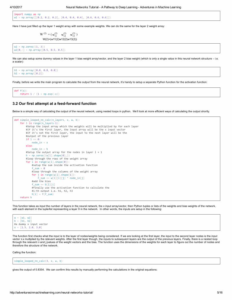
import numpy as np w1 = np.array([[0.2, 0.2, 0.2], [0.4, 0.4, 0.4], [0.6, 0.6, 0.6]])
Here I have just filled up the layer 1 weight array with some example weights. We can do the same for the layer 2 weight array:
w2 = np.zeros((1, 3)) w2[0,:] = np.array([0.5, 0.5, 0.5])
We can also setup some dummy values in the layer 1 bias weight array/vector, and the layer 2 bias weight (which is only a single value in this neural network structure – i.e.a scalar):
b1 = np.array([0.8, 0.8, 0.8]) b2 = np.array([0.2])
Finally, before we write the main program to calculate the output from the neural network, it’s handy to setup a separate Python function for the activation function:
def f(x): return 1 / (1 + np.exp(‐x))
3.2 Our first attempt at a feedforward function
Below is a simple way of calculating the output of the neural network, using nested loops in python. We’ll look at more efficient ways of calculating the output shortly.
def simple_looped_nn_calc(n_layers, x, w, b): for l in range(n_layers‐1): #Setup the input array which the weights will be multiplied by for each layer #If it's the first layer, the input array will be the x input vector #If it's not the first layer, the input to the next layer will be the #output of the previous layer if l == 0: node_in = x else: node_in = h #Setup the output array for the nodes in layer l + 1 h = np.zeros((w[l].shape[0],)) #loop through the rows of the weight array for i in range(w[l].shape[0]): #setup the sum inside the activation function f_sum = 0 #loop through the columns of the weight array for j in range(w[l].shape[1]): f_sum += w[l][i][j] * node_in[j] #add the bias f_sum += b[l][i] #finally use the activation function to calculate the #i‐th output i.e. h1, h2, h3 h[i] = f(f_sum) return h
This function takes as input the number of layers in the neural network, the x input array/vector, then Python tuples or lists of the weights and bias weights of the network,with each element in the tuple/list representing a layer in the network. In other words, the inputs are setup in the following:
w = [w1, w2] b = [b1, b2] #a dummy x input vector x = [1.5, 2.0, 3.0]
The function first checks what the input is to the layer of nodes/weights being considered. If we are looking at the first layer, the input to the second layer nodes is the inputvector multiplied by the relevant weights. After the first layer though, the inputs to subsequent layers are the output of the previous layers. Finally, there is a nested loopthrough the relevant and values of the weight vectors and the bias. The function uses the dimensions of the weights for each layer to figure out the number of nodes andtherefore the structure of the network.
Calling the function:
simple_looped_nn_calc(3, x, w, b)
gives the output of 0.8354. We can confirm this results by manually performing the calculations in the original equations:
= ( )W (2) w(2)11 w(2)
12 w(2)13
W(2)=(w11(2)w12(2)w13(2))
ll
xxii jj
(2)

4/10/2017 Neural Networks Tutorial A Pathway to Deep Learning Adventures in Machine Learning
http://adventuresinmachinelearning.com/neuralnetworkstutorial/ 6/16
3.3 A more efficient implementation
As was stated earlier – using loops isn’t the most efficient way of calculating the feed forward step in Python. This is because the loops in Python are notoriously slow. Analternative, more efficient mechanism of doing the feed forward step in Python and numpy will be discussed shortly. We can benchmark how efficient the algorithm is byusing the %timeit function in IPython, which runs the function a number of times and returns the average time that the function takes to run:
%timeit simple_looped_nn_calc(3, x, w, b)
Running this tells us that the looped feed forward takes . A result in the tens of microseconds sounds very fast, but when applied to very large practical NNs with100s of nodes per layer, this speed will become prohibitive, especially when training the network, as will become clear later in this tutorial. If we try a four layer neuralnetwork using the same code, we get significantly worse performance – in fact.
3.4 Vectorisation in neural networks
There is a way to write the equations even more compactly, and to calculate the feed forward process in neural networks more efficiently, from a computational perspective. Firstly, we can introduce a new variable which is the summated input into node of layer , including the bias term. So in the case of the first node in layer 2, isequal to:
where n is the number of nodes in layer 1. Using this notation, the unwieldy previous set of equations for the example three layer network can be reduced to:
Note the use of capital W to denote the matrix form of the weights. It should be noted that all of the elements in the above equation are now matrices / vectors. If you’reunfamiliar with these concepts, they will be explained more fully in the next section. Can the above equation be simplified even further? Yes, it can. We can forwardpropagate the calculations through any number of layers in the neural network by generalising:
Here we can see the general feed forward process, where the output of layer becomes the input to layer . We know that is simply the input layer and (where is the number of layers in the network) is the output of the output layer. Notice in the above equations that we have dropped references to the node
numbers and – how can we do this? Don’t we still have to loop through and calculate all the various node inputs and outputs?
The answer is that we can use matrix multiplications to do this more simply. This process is called “vectorisation” and it has two benefits – first, it makes the code lesscomplicated, as you will see shortly. Second, we can use fast linear algebra routines in Python (and other languages) rather than using loops, which will speed up ourprograms. Numpy can handle these calculations easily. First, for those who aren’t familiar with matrix operations, the next section is a brief recap.
3.5 Matrix multiplication
Let’s expand out in explicit matrix/vector form for the input layer (i.e. ):
For those who aren’t aware of how matrix multiplication works, it is a good idea to scrub up on matrix operations. There are many sites which cover this well. However, justquickly, when the weight matrix is multiplied by the input layer vector, each element in the of the weight matrix is multiplied by each element in the single
h (2)1h (2)2h (2)3(x)hW,b
= f(0.2 ∗ 1.5 + 0.2 ∗ 2.0 + 0.2 ∗ 3.0 + 0.8) = 0.8909
= f(0.4 ∗ 1.5 + 0.4 ∗ 2.0 + 0.4 ∗ 3.0 + 0.8) = 0.9677= f(0.6 ∗ 1.5 + 0.6 ∗ 2.0 + 0.6 ∗ 3.0 + 0.8) = 0.9909
= = f(0.5 ∗ 0.8909 + 0.5 ∗ 0.9677 + 0.5 ∗ 0.9909 + 0.2) = 0.8354h (3)1h1(2)=f(0.2∗1.5+0.2∗2.0+0.2∗3.0+0.8)=0.8909h2(2)=f(0.4∗1.5+0.4∗2.0+0.4∗3.0+0.8)=0.9677h3(2)=f(0.6∗1.5+0.6∗2.0+0.6∗3.0+0.8)=0.9909hW,b(x)=h1(3)=f(0.5∗0.8909+0.5∗0.9677
40μs40μs
70μs70μs
zi(l)z (l)i ii ll zz
= + + + = +z (2)1 w(1)11 x1 w(1)
12 x2 w(1)13 x3 b(1)1 ∑
j=1
nw(1)ij x i b(1)i
z1(2)=w11(1)x1+w12(1)x2+w13(1)x3+b1(1)=∑j=1nwij(1)xi+bi(1)
z (2)
h (2)
z (3)
(x)hW,b
= x +W (1) b(1)
= f( )z (2)
= +W (2) h (2) b(2)
= = f( )h (3) z (3)z(2)=W(1)x+b(1)h(2)=f(z(2))z(3)=W(2)h(2)+b(2)hW,b(x)=h(3)=f(z(3))
z (l+1)
h (l+1)= +W (l) h (l) b(l)
= f( )z (l+1)z(l+1)=W(l)h(l)+b(l)h(l+1)=f(z(l+1))
ll l+1l + 1 h(1)h (1) xxh(nl)h ( )n l nln l
ii jj
z(l+1)=W(l)h(l)+b(l)= +z (l+1) W (l) h (l) b(l) h(l)=x= xh (l)
z (2) = +⎛
⎝
⎜⎜⎜
w(1)11
w(1)21
w(1)31
w(1)12
w(1)22
w(1)32
w(1)13
w(1)23
w(1)33
⎞
⎠
⎟⎟⎟⎛
⎝⎜x1x2x3
⎞
⎠⎟
⎛
⎝
⎜⎜⎜
b(1)1b(1)2b(1)3
⎞
⎠
⎟⎟⎟
= +⎛
⎝
⎜⎜⎜
+ +w(1)11 x1 w(1)
12 x2 w(1)13 x3
+ +w(1)21 x1 w(1)
22 x2 w(1)23 x3
+ +w(1)31 x1 w(1)
32 x2 w(1)33 x3
⎞
⎠
⎟⎟⎟
⎛
⎝
⎜⎜⎜
b(1)1b(1)2b(1)3
⎞
⎠
⎟⎟⎟
=⎛
⎝
⎜⎜⎜
+ + +w(1)11 x1 w(1)
12 x2 w(1)13 x3 b(1)1
+ + +w(1)21 x1 w(1)
22 x2 w(1)23 x3 b(1)2
+ + +w(1)31 x1 w(1)
32 x2 w(1)33 x3 b(1)3
⎞
⎠
⎟⎟⎟
z(2)=(w11(1)w12(1)w13(1)w21(1)w22(1)w23(1)w31(1)w32(1)w33(1))(x1x2x3)+(b1(1)b2(1)b3(1))=(w11(1)x1+w12(1)x2+w13(1)x3w21(1)x1+w22(1)x2+w23(1)x3w31(1)x1+w32
rowrowcolumn

4/10/2017 Neural Networks Tutorial A Pathway to Deep Learning Adventures in Machine Learning
http://adventuresinmachinelearning.com/neuralnetworkstutorial/ 7/16
of the input vector, then summed to create a new (3 x 1) vector. Then you can simply add the bias weights vector to achieve the final result.
You can observe how each row of the final result above corresponds to the argument of the activation function in the original nonmatrix set of equations above. If theactivation function is capable of being applied elementwise (i.e. to each row separately in the vector), then we can do all our calculations using matrices andvectors rather than slow Python loops. Thankfully, numpy allows us to do just that, with reasonably fast matrix operations and elementwise functions. Let’s have a look at amuch more simplified (and faster) version of the simple_looped_nn_calc:
def matrix_feed_forward_calc(n_layers, x, w, b): for l in range(n_layers‐1): if l == 0: node_in = x else: node_in = h z = w[l].dot(node_in) + b[l] h = f(z) return h
Note line 7 where the matrix multiplication occurs – if you just use the symbol when multiplying the weights by the node input vector in numpy it will attempt to performsome sort of elementwise multiplication, rather than the true matrix multiplication that we desire. Therefore you need to use the a.dot(b) notation when performing matrixmultiplication in numpy.
If we perform %timeit again using this new function and a simple 4 layer network, we only get an improvement of (a reduction from to ). However, if we increase the size of the 4 layer network to layers of 1001005010 nodes the results are much more impressive. The Python looped based method takes awhopping – note, that is milliseconds, and the vectorised implementation only takes to forward propagate through the neural network. By usingvectorised calculations instead of Python loops we have increased the efficiency of the calculation 500 fold! That’s a huge improvement. There is even the possibility offaster implementations of matrix operations using deep learning packages such as TensorFlow and Theano which utilise your computer’s GPU (rather than the CPU), thearchitecture of which is more suited to fast matrix computations. However, that is a topic for later posts.
That brings us to an end of the feedforward introduction for neural networks. The next section will deal with how to actually train a neural network so that it can performclassification tasks, using gradient descent and backpropagation.
4 Gradient descent and optimisationAs mentioned in Section 1, the setting of the values of the weights which link the layers in the network is what constitutes the training of the system. In supervised learning,the idea is to reduce the error between the input and the desired output. So if we have a neural network with one output layer, and given some input we want the neuralnetwork to output a 2, yet the network actually produces a 5, a simple expression of the error is . For the mathematically minded, this would bethe norm of the error (don’t worry about it if you don’t know what this is).
The idea of supervised learning is to provide many inputoutput pairs of known data and vary the weights based on these samples so that the error expression is minimised.We can specify these inputoutput pairs as where is the number of training samples that we have on handto train the weights of the network. Each of these inputs or outputs can be vectors – that is is not necessarily just one value, it could be an dimensional series ofvalues. For instance, let’s say that we’re training a spamdetection neural network – in such a case could be a count of all the different significant words in an emaile.g.:
in this case could be a single scalar value, either a 1 or a 0 to designate whether the email is spam or not. Or, in other applications it could be a dimensionalvector. As an example, say we have input that is a vector of the pixel greyscale readings of a photograph. We also have an output that is a 26 dimensional vector thatdesignates, with a 1 or 0, what letter of the alphabet is shown in the photograph i.e. for a, for b and so on. This 26dimensional output vector could be used to classify letters in photographs.
In training the network with these pairs, the goal is to get the neural network better and better at predicting the correct given . This is performed by varyingthe weights so as to minimize the error. How do we know how to vary the weights, given an error in the output of the network? This is where the concept of gradientdescent comes in handy. Consider the diagram below:
columncolumn
z(1)z (1)
∗∗
24μs24μs 70μs70μs 46μs46μs
41ms41ms 84μs84μs
xxabs(2−5)=3abs(2 − 5) = 3
L1L1
{(x(1),y(1)),…,(x(m),y(m))}{( , ),… , ( , )}x (1) y (1) x (m) y (m) mmx(1)x (1) NN
x(1)x (1)
x (1) =
⎛
⎝
⎜⎜⎜⎜⎜⎜⎜⎜⎜
No. of“prince”No. of“nigeria”
No. of“extension”
⋮No. of“mum”No. of“burger”
⎞
⎠
⎟⎟⎟⎟⎟⎟⎟⎟⎟
=
⎛
⎝
⎜⎜⎜⎜⎜⎜⎜⎜⎜
220
⋮01
⎞
⎠
⎟⎟⎟⎟⎟⎟⎟⎟⎟
x(1)=(No.of“prince”No.of“nigeria”No.of“extension”⋮No.of“mum”No.of“burger”)=(220⋮01)
y(1)y (1) KKxx yy
(1,0,…,0)(1, 0,… , 0) (0,1,…,0)(0, 1,… , 0)
(x,y)(x, y) yy xx

4/10/2017 Neural Networks Tutorial A Pathway to Deep Learning Adventures in Machine Learning
http://adventuresinmachinelearning.com/neuralnetworkstutorial/ 8/16
Figure 8. Simple, onedimensional gradient descent
In this diagram we have a blue plot of the error depending on a single scalar weight value, . The minimum possible error is marked by the black cross, but we don’t knowwhat value gives that minimum error. We start out at a random value of , which gives an error marked by the red dot on the curve labelled with “1”. We need tochange in a way to approach that minimum possible error, the black cross. One of the most common ways of approaching that value is called gradient descent.
To proceed with this method, first the gradient of the error with respect to is calculated at point “1”. For those who don’t know, the gradient is the slope of the error curveat that point. It is shown in the diagram above by the black arrow which “pierces” point “1”. The gradient also gives directional information – if it is positive with respect to anincrease in , a step in that direction will lead to an increase in the error. If it is negative with respect to an increase in (as it is in the diagram above), a step in that willlead to a decrease in the error. Obviously, we wish to make a step in that will lead to a decrease in the error. The magnitude of the gradient or the “steepness” of theslope, gives an indication of how fast the error curve or function is changing at that point. The higher the magnitude of the gradient, the faster the error is changing at thatpoint with respect to .
The gradient descent method uses the gradient to make an informed step change in to lead it towards the minimum of the error curve. This is an iterative method, thatinvolves multiple steps. Each time, the value is updated according to:
Here denotes the new position, denotes the current or old position, is the gradient of the error at and is the stepsize. The step size will determine how quickly the solution converges on the minimum error. However, this parameter has to be tuned – if it is too large, you can imaginethe solution bouncing around on either side of the minimum in the above diagram. This will result in an optimisation of that does not converge. As this iterative algorithmapproaches the minimum, the gradient or change in the error with each step will reduce. You can see in the graph above that the gradient lines will “flatten out” as thesolution point approaches the minimum. As the solution approaches the minimum error, because of the decreasing gradient, it will result in only small improvements to theerror. When the solution approaches this “flattening” out of the error we want to exit the iterative process. This exit can be performed by either stopping after a certainnumber of iterations or via some sort of “stop condition”. This stop condition might be when the change in the error drops below a certain limit, often called the precision.
4.1 A simple example in code
Below is an example of a simple Python implementation of gradient descent for solving the minimum of the equation takenfrom Wikipedia. The gradient of this function is able to be calculated analytically (i.e. we can do it easily using calculus, which we can’t do with many real world applications)and is . This means at every value of , we can calculate the gradient of the function by using a simple equation. Again, using calculus wecan know that the exact minimum of this equation is .
x_old = 0 # The value does not matter as long as abs(x_new ‐ x_old) > precision x_new = 6 # The algorithm starts at x=6 gamma = 0.01 # step size precision = 0.00001
def df(x): y = 4 * x**3 ‐ 9 * x**2 return y
while abs(x_new ‐ x_old) > precision: x_old = x_new x_new += ‐gamma * df(x_old)
print("The local minimum occurs at %f" % x_new)
This function prints “The local minimum occurs at 2.249965”, which agrees with the exact solution within the precision. This code implements the weight adjustmentalgorithm that I showed above, and can be seen to find the minimum of the function correctly within the given precision. This is a very simple example of gradient descent,and finding the gradient works quite differently when training neural networks. However, the main idea remains – we figure out the gradient of the neural network then adjustthe weights in a step to try to get closer to the minimum error that we are trying to find. Another difference between this toy example of gradient descent is that the weightvector is multidimensional, and therefore the gradient descent method must search a multidimensional space for the minimum point.
The way we figure out the gradient of a neural network is via the famous backpropagation method, which will be discussed shortly. First however, we have to look at theerror function more closely.
4.2 The cost function
Previously, we’ve talked about iteratively minimising the error of the output of the neural network by varying the weights in gradient descent. However, as it turns out, there isa mathematically more generalised way of looking at things that allows us to reduce the error while also preventing things like overfitting (this will be discussed more in laterarticles). This more general optimisation formulation revolves around minimising what’s called the cost function. The equivalent cost function of a single training pair (
, ) in a neural network is:
This shows the cost function of the training sample, where is the output of the final layer of the neural network i.e. the output of the neural network. I’ve alsorepresented as to highlight the prediction of the neural network given . The two vertical lines represent the norm of the error, or what is
wwww ww
ww
ww
ww wwww
ww
wwww
= – α ∗ ∇errorwnew woldwnew=wold–α∗∇error
wnewwnew ww woldwold ww ∇error∇error woldwold αααα
ww
f(x)=x4–3x3+2f(x) = – 3 + 2x4 x3
f′(x)=4x3–9x2(x) = 4 – 9f ′ x3 x2 xxx=2.25x = 2.25
xzxz yzyz
J(w, b, x, y) = ∥ – ( )12
yz h ( )n l xz ∥2
= ∥ – ( )12
yz ypred xz ∥2
J(w,b,x,y)=12∥yz–h(nl)(xz)∥2=12∥yz–ypred(xz)∥2
zthzth h(nl)h ( )n l
h(nl)h ( )n l ypredypred xzxz L2L2

4/10/2017 Neural Networks Tutorial A Pathway to Deep Learning Adventures in Machine Learning
http://adventuresinmachinelearning.com/neuralnetworkstutorial/ 9/16
known as the sumofsquares error (SSE). SSE is a very common way of representing the error of a machine learning system. Instead of taking just the absolute error , we use the square of the error. There are many reasons why the SSE is often used which will not be discussed here – suffice to say
that this is a very common way of representing the errors in machine learning. The out the front is just a constant added that tidies things up when we differentiate thecost function, which we’ll be doing when we perform backpropagation.
Note that the formulation for the cost function above is for a single training pair. We want to minimise the cost function over all of our training pairs. Therefore,we want to find the minimum *mean squared error* (MSE) over all the training samples:
So, how do you use the cost function above to train the weights of our network? Using gradient descent and backpropagation. First, let’s look at gradient descent moreclosely in neural networks.
4.3 Gradient descent in neural networks
Gradient descent for every weight and every bias in the neural network looks like the following:
Basically, the equation above is similiar to the previously shown gradient descent algorithm: . The new and old subscriptsare missing, but the values on the left side of the equation are new and the values on the right side are old. Again, we have an iterative process whereby the weights areupdated in each iteration, this time based on the cost function .
The values and are the partial derivatives of the single sample cost function based on the weight values. What does this mean? Recall that for the
simple gradient descent example mentioned previously, each step depends on the slope of the error/cost term with respect to the weights. Another word for slope orgradient is the derivative. A normal derivative has the notation . If in this instance is a vector, then such a derivative will also be a vector, displaying the gradient inall the dimensions of .
4.4 A two dimensional gradient descent example
Let’s take the example of a standard twodimensional gradient descent problem. Below is a diagram of an iterative twodimensional gradient descent run:
Figure 9. Twodimensional gradient descent
The blue lines in the above diagram are the contour lines of the cost function – designating regions with an error value that is approximately the same. As can be observedin the diagram above, each step ( ) in the gradient descent involves a gradient or derivative that is an arrow/vector. This vector spans both the
dimensions, as the solution works its way towards the minimum in the centre. So, for instance, the derivative evaluated at might be , where the derivative is a vector to designate the two directions. The partial derivative in this case would be a scalar –
in other words, it is the gradient in only one direction of the search space ( ). In gradient descent, it is often the case that the partial derivative of all the possible searchdirections are calculated, then “gathered up” to determine a new, complete, step direction.
In neural networks, we don’t have a simple cost function where we can easily evaluate the gradient, like we did in our toy gradient descent example (). In fact, things are even trickier. While we can compare the output of the neural network to our expected training value, and
feasibly look at how changing the weights of the output layer would change the cost function for the sample (i.e. calculating the gradient), how on earth do we do that for allthe hidden layers of the network?
The answer to that is the backpropagation method. This method allows us to “share” the cost function or error to all the weights in the network – or in other words, it allowsus to determine how much of the error is caused by any given weight.
4.5 Backpropagation in depth
In this section, I’m going to delve into the maths a little. If you’re wary of the maths of how backpropagation works, then it may be best to skip this section. Thenext section will show you how to implement backpropagation in code – so if you want to skip straight on to using this method, feel free to skip the rest of this section.However, if you don’t mind a little bit of maths, I encourage you to push on to the end of this section as it will give you a good depth of understanding in training neural
pred
abs(ypred(xz)–yz)abs( ( )– )ypred xz yz121
2
(x,y)(x, y) mm
J(w, b) = ∥ – ( )1m
∑z=0
m 12
yz h ( )n l xz ∥2
= J(W, b, , )1m
∑z=0
mx (z) y (z)
J(w,b)=1m∑z=0m12∥yz–h(nl)(xz)∥2=1m∑z=0mJ(W,b,x(z),y(z))
JJ
w(ij)(l)w(l)(ij) bi(l)b(l)i
w(l)ij
b(l)i
= – α J(w, b)w(l)ij
∂
∂w(l)ij
= – α J(w, b)b(l)i∂
∂b(l)iwij(l)=wij(l)–α∂∂wij(l)J(w,b)bi(l)=bi(l)–α∂∂bi(l)J(w,b)
wnew=wold–α∗∇error= – α ∗ ∇errorwnew wold
J(w,b)J(w, b)
∂∂wij(l)∂∂w(l)
ij
∂∂bi(l)∂∂b(l)i
ddxddx xx
xx
p1→p2→p3→ →p1 p2 p3[x1,x2][ , ]x1 x2 p1p1
ddx=[2.1,0.7]= [2.1, 0.7]ddx ∂∂x1∂
∂x1→[2.1]→ [2.1]
x1x1
f(x)=x4–3x3+2f(x) = – 3 + 2x4 x3 y(z)y (z)

4/10/2017 Neural Networks Tutorial A Pathway to Deep Learning Adventures in Machine Learning
http://adventuresinmachinelearning.com/neuralnetworkstutorial/ 10/16
networks. This will be invaluable to understanding some of the key ideas in deep learning, rather than just being a code cruncher who doesn’t really understand how thecode works.
First let’s recall some of the foundational equations from Section 3 for the following three layer neural network:
Figure 10. Three layer neural network (again)
The output of this neural network can be calculated by:
We can also simplify the above to by defining as:
Let’s say we want to find out how much a change in the weight has on the cost function . This is to evaluate . To do so, we have to use
something called the chain function:
If you look at the terms on the right – the numerators “cancel out” the denominators, in the same way that . Therefore we can construct
by stringing together a few partial derivatives (which are quite easy, thankfully). Let’s start with :
The partial derivative of with respect only operates on one term within the parentheses, , as all the other terms don’t vary at all
when does. The derivative of a constant is 1, therefore collapses to just , which is simply the output of the
second node in layer 2.
The next partial derivative in the chain is , which is the partial derivative of the activation function of the output node. Because of the requirement
to be able to derive this derivative, the activation functions in neural networks need to be differentiable. For the common sigmoid activation function (shown in Section 2.1),the derivative is:
Where is the activation function. So far so good – now we have to work out how to deal with the first term . Remember that is
the mean squared error loss function, which looks like (for our case):
Here is the training target for the output node. Again using the chain rule:
(x) = = f( + + + )hW,b h (3)1 w(2)11 h
(2)1 w(2)
12 h(2)2 w(2)
13 h(2)3 b(2)1
hW,b(x)=h1(3)=f(w11(2)h1(2)+w12(2)h2(2)+w13(2)h3(2)+b1(2))
h1(3)=f(z1(2))= f( )h (3)1 z (2)1 z1(2)z (2)1
= + + +z (2)1 w(1)11 h
(2)1 w(1)
12 h(2)2 w(1)
13 h(2)3 b(1)1
z1(2)=w11(1)h1(2)+w12(1)h2(2)+w13(1)h3(2)+b1(1)
w12(2)w(2)12 JJ ∂J∂w12(2)∂J
∂w(2)12
=∂J
∂w(2)12
∂J
∂h (3)1
∂h (3)1∂z (2)1
∂z (2)1
∂w(2)12
∂J∂w12(2)=∂J∂h1(3)∂h1(3)∂z1(2)∂z1(2)∂w12(2)
2552=22=1= = 12552
22
∂J∂w12(2)∂J∂w(2)
12
∂z1(2)∂w12(2)∂z (2)1
∂w(2)12
∂z (2)1
∂w(2)12
= ( + + + )∂
∂w(2)12
w(1)11 h
(2)1 w(1)
12 h(2)2 w(1)
13 h(2)3 b(1)1
= ( )∂
∂w(2)12
w(1)12 h
(2)2
= h (2)2∂z1(2)∂w12(2)=∂∂w12(2)(w11(1)h1(2)+w12(1)h2(2)+w13(1)h3(2)+b1(1))=∂∂w12(2)(w12(1)h2(2))=h2(2)
z1(2)z (2)1 w12(2)w(2)12 w12(1)h2(2)w(1)
12 h(2)2
w12(2)w(2)12 ∂∂w12(2)(w12(1)h2(2))( )∂
∂w(2)12
w(1)12 h
(2)2 h2(2)h (2)2
∂h1(3)∂z1(2)∂h (3)1∂z (2)1
h1(3)h (3)1
= (z) = f(z)(1 − f(z))∂h∂z
f ′
∂h∂z=f′(z)=f(z)(1−f(z))
f(z)f(z) ∂J∂h1(3)∂J∂h (3)1
J(w,b,x,y)J(w, b, x, y)
J(w, b, x, y) = ∥ – ( )12
y1 h (3)1 z (2)1 ∥2
J(w,b,x,y)=12∥y1–h1(3)(z1(2))∥2
y1y1
Let u =∥ – ( ) ∥ and J =y1 h (3)1 z (2)112u2
Using = :∂J∂h
∂J∂u
∂u∂h
= −( – )∂J∂h
y1 h (3)1

4/10/2017 Neural Networks Tutorial A Pathway to Deep Learning Adventures in Machine Learning
http://adventuresinmachinelearning.com/neuralnetworkstutorial/ 11/16
So we’ve now figured out how to calculate , at least for the weights connecting the output layer. Before we move to any hidden layers (i.e. layer 2 in our
example case), let’s introduce some simplifications to tighten up our notation and introduce :
Where is the node number of the output layer. In our selected example there is only one such layer, therefore always in this case. Now we can write the completecost function derivative as:
Where, for the output layer in our case, = 2 and remains the node number.
4.6 Propagating into the hidden layers
What about for weights feeding into any hidden layers (layer 2 in our case)? For the weights connecting the output layer, the derivativemade sense, as the cost function can be directly calculated by comparing the output layer to the training data. The output of the hidden nodes, however, have no such directreference, rather, they are connected to the cost function only through mediating weights and potentially other layers of nodes. How can we find the variation in the costfunction from changes to weights embedded deep within the neural network? As mentioned previously, we use the backpropagation method.
Now that we’ve done the hard work using the chain rule, we’ll now take a more graphical approach. The term that needs to propagate back through the network is the term, as this is the network’s ultimate connection to the cost function. What about node j in the second layer (hidden layer)? How does it contribute to in
our test network? It contributes via the weight – see the diagram below for the case of and .
Figure 11. Simple backpropagation illustration
As can be observed from above, the output layer is communicated to the hidden node by the weight of the connection. In the case where there is only one output layernode, the generalised hidden layer is defined as:
Where is the node number in layer . What about the case where there are multiple output nodes? In this case, the weighted sum of all the communicated errors are
taken to calculate , as shown in the diagram below:
Figure 12. Backpropagation illustration with multipleoutputs
As can be observed from the above, each value from the output layer is included in the sum used to calculate , but each output is weighted according to the
appropriate value. In other words, node 1 in layer 2 contributes to the error of three output nodes, therefore the measured error (or cost function value) at eachof these nodes has to be “passed back” to the value for this node. Now we can develop a generalised expression for the values for nodes in the hidden layers:
Let u=∥y1–h1(3)(z1(2))∥ and J=12u2Using ∂J∂h=∂J∂u∂u∂h:∂J∂h=−(y1–h1(3))
∂J∂w12(2)∂J∂w(2)
12
δδ
= −( – ) ⋅ ( )δ( )n li yi h ( )n l
i f ′ z ( )n li
δi(nl)=−(yi–hi(nl))⋅f′(zi(nl))
ii i=1i = 1
J(W, b, x, y)∂
∂W (l)ij
= h (l)j δ(l+1)i
∂∂Wij(l)J(W,b,x,y)=hj(l)δi(l+1)
ll ii
∂J∂h=−(yi–hi(nl))= −( – )∂J∂h yi h ( )n l
i
δi(nl)δ( )n li δi(nl)δ( )n l
iwij(2)w(2)
ij j=1j = 1 i=1i = 1
δδδδ
= (δ(l)j δ(l+1)1 w(l)1j f
′ zj ) (l)
δj(l)=δ1(l+1)w1j(l) f′(zj)(l)
jj llδj(l)δ(l)j
δδ δ1(2)δ(2)1 δδwi1(2)w(2)
i1δδ δδ
= ( ) ( )δ(l)j ∑i=1
s (l+1)
w(l)ij δ
(l+1)i f ′ z (l)j
δj(l)=(∑i=1s(l+1)wij(l)δi(l+1)) f′(zj(l))
j l i l + 1

4/10/2017 Neural Networks Tutorial A Pathway to Deep Learning Adventures in Machine Learning
http://adventuresinmachinelearning.com/neuralnetworkstutorial/ 12/16
Where is the node number in layer and is the node number in layer (which is the same notation we have used from the start). The value is thenumber of nodes in layer .
So we now know how to calculate:
as shown previously. What about the bias weights? I’m not going to derive them as I did with the normal weights in the interest of saving time / space. However, the readershouldn’t have too many issues following the same steps, using the chain rule, to arrive at:
Great – so we now know how to perform our original gradient descent problem for neural networks:
However, to perform this gradient descent training of the weights, we would have to resort to loops within loops. As previously shown in Section 3.4 of this neural networktutorial, performing such calculations in Python using loops is slow for large networks. Therefore, we need to figure out how to vectorise such calculations, which the nextsection will show.
4.7 Vectorisation of backpropagation
To consider how to vectorise the gradient descent calculations in neural networks, let’s first look at a naïve vectorised version of the gradient of the cost function (warning:this is not in a correct form yet!):
Now, let’s look at what element of the above equations. What does look like? Pretty simple, just a vector, where is the number of nodes in layer .What does the multiplication of look like? Well, because we know that must be the same size of the weight matrix , we
know that the outcome of must also be the same size as the weight matrix for layer . In other words it has to be of size .
We know that has the dimension and that has the dimension of . The rules of matrix multiplication show that a matrixof dimension multiplied by a matrix of dimension will have a product matrix of size . If we perform a straight multiplicationbetween and , the number of columns of the first vector (i.e. 1 column) will not equal the number of rows of the second vector (i.e. 3 rows), therefore wecan’t perform a proper matrix multiplication. The only way we can get a proper outcome of size is by using a matrix transpose. A transpose swaps thedimensions of a matrix around e.g. a sized vector becomes a sized vector, and is denoted by a superscript of . Therefore, we can do thefollowing:
As can be observed below, by using the transpose operation we can arrive at the outcome we desired.
A final vectorisation that can be performed is during the weighted addition of the errors in the backpropagation step:
The symbol in the above designates an elementbyelement multiplication (called the Hadamard product), not a matrix multiplication. Note that the matrix multiplication performs the necessary summation of the weights and values – the reader can check that this is the case.
4.8 Implementing the gradient descent step
Now, how do we integrate this new vectorisation into the gradient descent steps of our soontobe coded algorithm? First, we have to look again at the overall cost functionwe are trying to minimise (not just the samplebysample cost function shown in the preceding equation):
As we can observe, the total cost function is the mean of all the samplebysample cost function calculations. Also remember the gradient descent calculation (showing theelementbyelement version along with the vectorised version):
jj ll ii l+1l + 1 s(l+1)s (l+1)(l+1)(l + 1)
J(W, b, x, y) =∂
∂W (l)ij
h (l)j δ(l+1)i
∂∂Wij(l)J(W,b,x,y)=hj(l)δi(l+1)
J(W, b, x, y) =∂
∂b(l)iδ(l+1)i
∂∂bi(l)J(W,b,x,y)=δi(l+1)
w(l)ij
b(l)i
= – α J(w, b)w(l)ij
∂
∂w(l)ij
= – α J(w, b)b(l)i∂
∂b(l)iwij(l)=wij(l)–α∂∂wij(l)J(w,b)bi(l)=bi(l)–α∂∂bi(l)J(w,b)
∂J∂W (l)
∂J∂b(l)
= h (l) δ(l+1)
= δ(l+1)
∂J∂W(l)=h(l)δ(l+1)∂J∂b(l)=δ(l+1)
h(l)h (l) (sl×1)( × 1)s l sls l llh(l)δ(l+1)h (l) δ(l+1) α×∂J∂W(l)α × ∂J
∂W (l) W(l)W (l)
h(l)δ(l+1)h (l) δ(l+1) ll (sl+1×sl)( × )s l+1 s l
δ(l+1)δ(l+1) (sl+1×1)( × 1)s l+1 h(l)h (l) (sl×1)( × 1)s l(n×m)(n × m) (o×p)(o × p) (n×p)(n × p)
h(l)h (l) δ(l+1)δ(l+1)(sl+1×sl)( × )s l+1 s l
(sl×1)( × 1)s l (1×sl)(1 × )s l TT
( = ( × 1) × (1 × ) = ( × )δ(l+1) h (l) )T s l+1 s l s l+1 s lδ(l+1)(h(l))T=(sl+1×1)×(1×sl)=(sl+1×sl)
= ( ) ( ) = (( ) ∙ ( )δ(l)j ∑i=1
s (l+1)
w(l)ij δ
(l+1)i f ′ z (l)j W (l) )T δ(l+1) f ′ z (l)
δj(l)=(∑i=1s(l+1)wij(l)δi(l+1)) f′(zj(l))=((W(l))Tδ(l+1))∙f′(z(l))
∙∙((W(l))Tδ(l+1))(( )W (l) )T δ(l+1) δδ
J(w, b) = J(W, b, , )1m
∑z=0
mx (z) y (z)
J(w,b)=1m∑z=0mJ(W,b,x(z),y(z))
∂

4/10/2017 Neural Networks Tutorial A Pathway to Deep Learning Adventures in Machine Learning
http://adventuresinmachinelearning.com/neuralnetworkstutorial/ 13/16
So that means as we go along through our training samples or batches, we have to have a term that is summing up the partial derivatives of the individual sample costfunction calculations. This term will gather up all the values for the mean calculation. Let’s call this “summing up” term . Likewise, the equivalent bias term canbe called . Therefore, at each sample iteration of the final training algorithm, we have to perform the following steps:
By performing the above operations at each iteration, we slowly build up the previously mentioned sum (and
the same for ). Once all the samples have been iterated through, and the values have been summed up, we update the weight parameters :
4.9 The final gradient descent algorithm
So, no we’ve finally made it to the point where we can specify the entire backpropagationbased gradient descent training of our neural networks. It has taken quite a fewsteps to show, but hopefully it has been instructive. The final backpropagation algorithm is as follows:
Randomly initialise the weights for each layer While iterations < iteration limit:1. Set and to zero2. For samples 1 to m:a. Perform a feed foward pass through all the layers. Store the activation function outputs b. Calculate the value for the output layerc. Use backpropagation to calculate the values for layers 2 to d. Update the and for each layer3. Perform a gradient descent step using:
As specified in the algorithm above, we would repeat the gradient descent routine until we are happy that the average cost function has reached a minimum. At this point,our network is trained and (ideally) ready for use.
The next part of this neural networks tutorial will show how to implement this algorithm to train a neural network that recognises handwritten digits.
5 Implementing the neural network in PythonIn the last section we looked at the theory surrounding gradient descent training in neural networks and the backpropagation method. In this article, we are going to applythat theory to develop some code to perform training and prediction on the MNIST dataset. The MNIST dataset is a kind of goto dataset in neural network and deeplearning examples, so we’ll stick with it here too. What it consists of is a record of images of handwritten digits with associated labels that tell us what the digit is. Each imageis 8 x 8 pixels in size, and the image data sample is represented by 64 data points which denote the pixel intensity. In this example, we’ll be using the MNIST datasetprovided in the Python Machine Learning library called scikit learn. An example of the image (and the extraction of the data from the scikit learn dataset) is shown in thecode below (for an image of 1):
from sklearn.datasets import load_digits digits = load_digits() print(digits.data.shape) import matplotlib.pyplot as plt plt.gray() plt.matshow(digits.images[1]) plt.show()
w(l)ij
W (l)
= – α J(w, b)w(l)ij
∂
∂w(l)ij
= – α J(w, b)W (l) ∂∂W (l)
= – α [ J(w, b, , )]W (l) 1m
∑z=1
m ∂∂W (l)
x (z) y (z)
wij(l)=wij(l)–α∂∂wij(l)J(w,b)W(l)=W(l)–α∂∂W(l)J(w,b)=W(l)–α[1m∑z=1m∂∂W(l)J(w,b,x(z),y(z))]
ΔW(l)ΔW (l)
Δb(l)Δb(l)
ΔW (l)
Δb(l)
= Δ + J(w, b, , )W (l) ∂∂W (l)
x (z) y (z)
= Δ + (W (l) δ(l+1) h (l) )T
= Δ +b(1) δ(l+1)ΔW(l)=ΔW(l)+∂∂W(l)J(w,b,x(z),y(z))=ΔW(l)+δ(l+1)(h(l))TΔb(l)=Δb(1)+δ(l+1)
∑z=1m∂∂W(l)J(w,b,x(z),y(z))J(w, b, , )∑ mz=1
∂∂W (l) x (z) y (z)
bb ΔΔ
W (l)
b(l)
= – α [ Δ ]W (l) 1m
W (l)
= – α [ Δ ]b(l)1m
b(l)
W(l)=W(l)–α[1mΔW(l)]b(l)=b(l)–α[1mΔb(l)]
W(l)W (l)
ΔWΔW ΔbΔb
nln l h(l)h (l)δ(nl)δ( )n l
δ(l)δ(l) nl−1− 1n lΔW(l)ΔW (l) Δb(l)Δb(l)
W(l)=W(l)–α[1mΔW(l)]= – α [ Δ ]W (l) W (l) 1m W (l)
b(l)=b(l)–α[1mΔb(l)]= – α [ Δ ]b(l) b(l) 1m b(l)

4/10/2017 Neural Networks Tutorial A Pathway to Deep Learning Adventures in Machine Learning
http://adventuresinmachinelearning.com/neuralnetworkstutorial/ 14/16
Figure 13. MNIST digit “1”
The code above prints (1797, 64) to show the shape of input data matrix and the pixelated digit “1” in the image above. The code we are going to write in this neuralnetworks tutorial will try and estimate the digits that these pixels represent (using neural networks of course). First things first, we need to get the input data in shape. To doso, we need to do two things:
1. Scale the data2. Split the data into test and train sets
5.1 Scaling data
Why do we need to scale the input data? First, have a look at one of the dataset pixel representations:
digits.data[0,:] Out[2]: array([ 0., 0., 5., 13., 9., 1., 0., 0., 0., 0., 13., 15., 10., 15., 5., 0., 0., 3., 15., 2., 0., 11., 8., 0., 0., 4., 12., 0., 0., 8., 8., 0., 0., 5., 8., 0., 0., 9., 8., 0., 0., 4., 11., 0., 1., 12., 7., 0., 0., 2., 14., 5., 10., 12., 0., 0., 0., 0., 6., 13., 10., 0., 0., 0.])
Notice that the input data ranges from 0 up to 15? It’s standard practice to scale the input data so that it all fits mostly between either 0 to 1 or with a small range centredaround 0 i.e. 1 to 1. Why? Well, it can help the convergence of the neural network and is especially important if we are combining different data types. Thankfully, this iseasily done using scikit learn:
from sklearn.preprocessing import StandardScaler X_scale = StandardScaler() X = X_scale.fit_transform(digits.data) X[0,:] Out[3]: array([ 0. , ‐0.33501649, ‐0.04308102, 0.27407152, ‐0.66447751, ‐0.84412939, ‐0.40972392, ‐0.12502292, ‐0.05907756, ‐0.62400926, 0.4829745 , 0.75962245, ‐0.05842586, 1.12772113, 0.87958306, ‐0.13043338, ‐0.04462507, 0.11144272, 0.89588044, ‐0.86066632, ‐1.14964846, 0.51547187, 1.90596347, ‐0.11422184, ‐0.03337973, 0.48648928, 0.46988512, ‐1.49990136, ‐1.61406277, 0.07639777, 1.54181413, ‐0.04723238, 0. , 0.76465553, 0.05263019, ‐1.44763006, ‐1.73666443, 0.04361588, 1.43955804, 0. , ‐0.06134367, 0.8105536 , 0.63011714, ‐1.12245711, ‐1.06623158, 0.66096475, 0.81845076, ‐0.08874162, ‐0.03543326, 0.74211893, 1.15065212, ‐0.86867056, 0.11012973, 0.53761116, ‐0.75743581, ‐0.20978513, ‐0.02359646, ‐0.29908135, 0.08671869, 0.20829258, ‐0.36677122, ‐1.14664746, ‐0.5056698 , ‐0.19600752])
The scikit learn standard scaler by default normalises the data by subtracting the mean and dividing by the standard deviation. As can be observed, most of the data pointsare centered around zero and contained within 2 and 2. This is a good starting point. There is no real need to scale the output data .
5.2 Creating test and training datasets
In machine learning, there is a phenomenon called “overfitting”. This occurs when models, during training, become too complex – they become really well adapted to predictthe training data, but when they are asked to predict something based on new data that they haven’t “seen” before, they perform poorly. In other words, the modelsdon’t generalise very well. To make sure that we are not creating models which are too complex, it is common practice to split the dataset into a training set and a test set.The training set is, obviously, the data that the model will be trained on, and the test set is the data that the model will be tested on after it has been trained. The amount oftraining data is always more numerous than the testing data, and is usually between 6080% of the total dataset.
Again, scikit learn makes this splitting of the data into training and testing sets easy:
from sklearn.model_selection import train_test_split y = digits.target X_train, X_test, y_train, y_test = train_test_split(X, y, test_size=0.4)
In this case, we’ve made the test set to be 40% of the total data, leaving 60% to train with. The train_test_split function in scikit learn pushes the data randomly into thedifferent datasets – in other words, it doesn’t take the first 60% of rows as the training set and the second 40% of rows as the test set. This avoids data collection artefactsfrom degrading the performance of the model.
yy

4/10/2017 Neural Networks Tutorial A Pathway to Deep Learning Adventures in Machine Learning
http://adventuresinmachinelearning.com/neuralnetworkstutorial/ 15/16
5.3 Setting up the output layer
As you would have been able to gather, we need the output layer to predict whether the digit represented by the input pixels is between 0 and 9. Therefore, a sensibleneural network architecture would be to have an output layer of 10 nodes, with each of these nodes representing a digit from 0 to 9. We want to train the network so thatwhen, say, an image of the digit “5” is presented to the neural network, the node in the output layer representing 5 has the highest value. Ideally, we would want to see anoutput looking like this: [0, 0, 0, 0, 0, 1, 0, 0, 0, 0]. However, in reality, we can settle for something like this: [0.01, 0.1, 0.2, 0.05, 0.3, 0.8, 0.4, 0.03, 0.25, 0.02]. In this case,we can take the maximum index of the output array and call that our predicted digit.
For the MNIST data supplied in the scikit learn dataset, the “targets” or the classification of the handwritten digits is in the form of a single number. We need to convert thatsingle number into a vector so that it lines up with our 10 node output layer. In other words, if the target value in the dataset is “1” we want to convert it into the vector: [0, 1,0, 0, 0, 0, 0, 0, 0, 0]. The code below does just that:
import numpy as np def convert_y_to_vect(y): y_vect = np.zeros((len(y), 10)) for i in range(len(y)): y_vect[i, y[i]] = 1 return y_vect
y_v_train = convert_y_to_vect(y_train) y_v_test = convert_y_to_vect(y_test) y_train[0], y_v_train[0] Out[8]: (1, array([ 0., 1., 0., 0., 0., 0., 0., 0., 0., 0.]))
As can be observed above, the MNIST target (1) has been converted into the vector [0, 1, 0, 0, 0, 0, 0, 0, 0, 0], which is what we want.
5.4 Creating the neural network
The next step is to specify the structure of the neural network. For the input layer, we know we need 64 nodes to cover the 64 pixels in the image. As discussed, we need 10output layer nodes to predict the digits. We’ll also need a hidden layer in our network to allow for the complexity of the task. Usually, the number of hidden layer nodes issomewhere between the number of input layers and the number of output layers. Let’s define a simple Python list that designates the structure of our network:
nn_structure = [64, 30, 10]
We’ll use sigmoid activation functions again, so let’s setup the sigmoid function and its derivative:
def f(x): return 1 / (1 + np.exp(‐x))
def f_deriv(x): return f(x) * (1 ‐ f(x))
Ok, so we now have an idea of what our neural network will look like. How do we train it? Remember the algorithm from Section 4.9 , which we’ll repeat here for ease ofaccess and review:
Randomly initialise the weights for each layer While iterations < iteration limit:1. Set and to zero2. For samples 1 to m:a. Perform a feed foward pass through all the layers. Store the activation function outputs b. Calculate the value for the output layerc. Use backpropagation to calculate the values for layers 2 to d. Update the and for each layer3. Perform a gradient descent step using:
So the first step is to initialise the weights for each layer. To make it easy to organise the various layers, we’ll use Python dictionary objects (initialised by {}). Finally, theweights have to be initialised with random values – this is to ensure that the neural network will converge correctly during training. We use the numpy library random_samplefunction to do this. The weight initialisation code is shown below:
import numpy.random as r def setup_and_init_weights(nn_structure): W = {} b = {} for l in range(1, len(nn_structure)): W[l] = r.random_sample((nn_structure[l], nn_structure[l‐1])) b[l] = r.random_sample((nn_structure[l],)) return W, b
The next step is to set the mean accumulation values and to zero (they need to be the same size as the weight and bias matrices):
W(l)W (l)
ΔWΔW ΔbΔb
nln l h(l)h (l)δ(nl)δ( )n l
δ(l)δ(l) nl−1− 1n lΔW(l)ΔW (l) Δb(l)Δb(l)
W(l)=W(l)–α[1mΔW(l)]= – α [ Δ ]W (l) W (l) 1m W (l)
b(l)=b(l)–α[1mΔb(l)]= – α [ Δ ]b(l) b(l) 1m b(l)
ΔWΔW ΔbΔb

4/10/2017 Neural Networks Tutorial A Pathway to Deep Learning Adventures in Machine Learning
http://adventuresinmachinelearning.com/neuralnetworkstutorial/ 16/16
def init_tri_values(nn_structure): tri_W = {} tri_b = {} for l in range(1, len(nn_structure)): tri_W[l] = np.zeros((nn_structure[l], nn_structure[l‐1])) tri_b[l] = np.zeros((nn_structure[l],)) return tri_W, tri_b
If we now step into the gradient descent loop, the first step is to perform a feed forward pass through the network. The code below is a variation on the feed forward functioncreated in Section 3:
def feed_forward(x, W, b): h = {1: x} z = {} for l in range(1, len(W) + 1): # if it is the first layer, then the input into the weights is x, otherwise, # it is the output from the last layer if l == 1: node_in = x else: node_in = h[l] z[l+1] = W[l].dot(node_in) + b[l] # z^(l+1) = W^(l)*h^(l) + b^(l) h[l+1] = f(z[l+1]) # h^(l) = f(z^(l)) return h, z
Finally, we have to then calculate the output layer delta and any hidden layer delta values to perform the backpropagation pass:
def calculate_out_layer_delta(y, h_out, z_out): # delta^(nl) = ‐(y_i ‐ h_i^(nl)) * f'(z_i^(nl)) return ‐(y‐h_out) * f_deriv(z_out)
def calculate_hidden_delta(delta_plus_1, w_l, z_l): # delta^(l) = (transpose(W^(l)) * delta^(l+1)) * f'(z^(l)) return np.dot(np.transpose(w_l), delta_plus_1) * f_deriv(z_l)
Now we can put all the steps together into the final function:
def train_nn(nn_structure, X, y, iter_num=3000, alpha=0.25): W, b = setup_and_init_weights(nn_structure) cnt = 0 m = len(y) avg_cost_func = [] print('Starting gradient descent for {} iterations'.format(iter_num)) while cnt < iter_num: if cnt%1000 == 0: print('Iteration {} of {}'.format(cnt, iter_num)) tri_W, tri_b = init_tri_values(nn_structure) avg_cost = 0 for i in range(len(y)): delta = {} # perform the feed forward pass and return the stored h and z values, to be used in the # gradient descent step h, z = feed_forward(X[i, :], W, b) # loop from nl‐1 to 1 backpropagating the errors for l in range(len(nn_structure), 0, ‐1): if l == len(nn_structure): delta[l] = calculate_out_layer_delta(y[i,:], h[l], z[l]) avg_cost += np.linalg.norm((y[i,:]‐h[l])) else: if l > 1: delta[l] = calculate_hidden_delta(delta[l+1], W[l], z[l]) # triW^(l) = triW^(l) + delta^(l+1) * transpose(h^(l)) tri_W[l] += np.dot(delta[l+1][:,np.newaxis], np.transpose(h[l][:,np.newaxis])) # trib^(l) = trib^(l) + delta^(l+1) tri_b[l] += delta[l+1] # perform the gradient descent step for the weights in each layer for l in range(len(nn_structure) ‐ 1, 0, ‐1): W[l] += ‐alpha * (1.0/m * tri_W[l]) b[l] += ‐alpha * (1.0/m * tri_b[l]) # complete the average cost calculation avg_cost = 1.0/m * avg_cost avg_cost_func.append(avg_cost) cnt += 1 return W, b, avg_cost_func
The function above deserves a bit of explanation. First, we aren’t setting a termination of the gradient descent process based on some change or precision of the costfunction. Rather, we are just running it for a set number of iterations (3,000 in this case) and we’ll monitor how the average cost function changes as we progress throughthe training (avg_cost_func list in the above code). In each iteration of the gradient descent, we cycle through each training sample (range(len(y)) and perform the feedforward pass and then the backpropagation. The backpropagation step is an iteration through the layers starting at the output layer and working backwards –
δ(nl)δ( )n l δ(l)δ(l)