neural network based vector hysteresis model and …maxwell.sze.hu/docs/a1.pdf · neural network...
TRANSCRIPT

Neural Network Based
Vector Hysteresis Model and the
Nondestructive Testing Method
by
Miklos KuczmannMSc in Electrical Engineering
supervisor
prof. Amalia Ivanyi
A thesis submitted to theBudapest University of Technology and Economics
for the degree ofDoctor of Philosophy
in Electrical Engineering
Department of Broadband Infocommunications and Electromagnetic TheoryBudapest University of Technology and Economics
Budapest2004

Contents
1 Introduction and the scope of my research 1
1.1 The proposed research activity . . . . . . . . . . . . . . . . . . . . . . . . 2
1.2 Acknowledgment . . . . . . . . . . . . . . . . . . . . . . . . . . . . . . . 3
2 Literature overview 4
2.1 Artificial neural networks . . . . . . . . . . . . . . . . . . . . . . . . . . . 4
2.1.1 Biological background . . . . . . . . . . . . . . . . . . . . . . . . 4
2.1.2 Structure and training of feedforward neural networks . . . . . . . 4
2.2 Preisach–type hysteresis models based on NN . . . . . . . . . . . . . . . 7
2.2.1 The classical scalar Preisach model . . . . . . . . . . . . . . . . . 7
2.2.2 The classical scalar Preisach model via NNs . . . . . . . . . . . . 10
2.2.3 Vector hysteresis modeling . . . . . . . . . . . . . . . . . . . . . . 12
2.3 The nondestructive testing method . . . . . . . . . . . . . . . . . . . . . 14
2.4 Formulation and potentials of the electromagnetic field problems . . . . . 15
2.5 The finite element method . . . . . . . . . . . . . . . . . . . . . . . . . . 17
2.5.1 Nodal finite elements . . . . . . . . . . . . . . . . . . . . . . . . . 18
2.5.2 Edge finite elements . . . . . . . . . . . . . . . . . . . . . . . . . 19
2.5.3 FEM in 2D using linear shape functions . . . . . . . . . . . . . . 20
2.5.4 FEM in 3D using linear shape functions . . . . . . . . . . . . . . 23
3 Neural network based hysteresis operator 25
3.1 The scalar hysteresis operator . . . . . . . . . . . . . . . . . . . . . . . . 25
3.1.1 Training sequence and preprocessing of measured data . . . . . . 25
3.1.2 Operation of the model . . . . . . . . . . . . . . . . . . . . . . . . 27
3.1.3 Properties of the scalar model . . . . . . . . . . . . . . . . . . . . 29
3.1.4 Scalar magnetic hysteresis measurement using LabVIEW . . . . . 31
3.2 The isotropic vector hysteresis operator . . . . . . . . . . . . . . . . . . . 34
3.2.1 Description of the model . . . . . . . . . . . . . . . . . . . . . . . 34
3.2.2 The identification process . . . . . . . . . . . . . . . . . . . . . . 34
3.2.3 Verification of the model . . . . . . . . . . . . . . . . . . . . . . . 39
3.3 The anisotropic vector hysteresis operator . . . . . . . . . . . . . . . . . 41
I

Miklos Kuczmann, PhD Theses 2004
3.3.1 Anisotropic model in 2D . . . . . . . . . . . . . . . . . . . . . . . 41
3.3.2 Anisotropic model in 3D . . . . . . . . . . . . . . . . . . . . . . . 44
3.3.3 The relation between the scalar and the vector Everett functions . 47
3.4 Some properties of the vector hysteresis characteristics . . . . . . . . . . 51
3.5 New scientific results . . . . . . . . . . . . . . . . . . . . . . . . . . . . . 53
4 Nonlinear FEM using edge finite elements 55
4.1 Problem definition and the FEM formulation . . . . . . . . . . . . . . . . 55
4.1.1 Time varying magnetic field problem in linear media . . . . . . . 56
4.1.2 Eddy current field in linear media . . . . . . . . . . . . . . . . . . 59
4.1.3 The T ,Ψ− Ψ formulation in hysteretic media . . . . . . . . . . . 65
4.2 Summary . . . . . . . . . . . . . . . . . . . . . . . . . . . . . . . . . . . 71
4.3 New scientific results . . . . . . . . . . . . . . . . . . . . . . . . . . . . . 71
5 Simulation of the built NDT measurement system 72
5.1 Description of the measurement system . . . . . . . . . . . . . . . . . . . 72
5.2 Applying the FluxSet sensor . . . . . . . . . . . . . . . . . . . . . . . . . 74
5.2.1 Preliminary measurements . . . . . . . . . . . . . . . . . . . . . . 74
5.2.2 Calibration of the sensor . . . . . . . . . . . . . . . . . . . . . . . 75
5.2.3 The lock–in amplifier . . . . . . . . . . . . . . . . . . . . . . . . . 77
5.2.4 NDT measurements . . . . . . . . . . . . . . . . . . . . . . . . . . 78
5.3 Applying the Hall–type sensor . . . . . . . . . . . . . . . . . . . . . . . . 81
5.3.1 Preliminary measurements and calibration . . . . . . . . . . . . . 81
5.3.2 NDT measurements . . . . . . . . . . . . . . . . . . . . . . . . . . 82
5.4 Conclusions of the measurements . . . . . . . . . . . . . . . . . . . . . . 83
5.5 Simulation of the installed NDT equipment . . . . . . . . . . . . . . . . . 86
5.5.1 Global–local model in 3D calculations . . . . . . . . . . . . . . . . 86
5.5.2 Simulation of the Hall sensor . . . . . . . . . . . . . . . . . . . . . 93
5.6 New scientific results . . . . . . . . . . . . . . . . . . . . . . . . . . . . . 97
6 Summary of the new scientific results 98
7 Conclusions and future developments 100
II

Notations
NN Neural Network
NDT Nondestructive Testing
FEM Finite Element Method
MSE Means Square Error
BP Backpropagation training method
PE Processing Element (neuron)
CAD Computer Aided Design
NI National Instruments
DAQ Data Acquisition
DC, AC Direct Current, Alternating Current
CC mode Constant Current mode of the power supply
W Weight matrix of a neural network
µ(α, β) Preisach distribution function
E(α, β) Everett function
F (α, β) Measured Everett function for the isotropic vector model
F (α, β, ϕ) Measured Everett function for the 2D anisotropic vector model
F (α, β, ϕ, ϑ) Measured Everett function for the 3D anisotropic vector model
Fm, Fnm Fourier coefficients of the measured anisotropic Everett function
Em, Enm Fourier coefficients of the identified anisotropic Everett function
H , HM, HB Hysteresis operator
ξ Parameter of a reversal hysteresis curve
γ(α, β) Relay operator
H, H Magnetic field intensity (scalar, vector)
M, M Magnetization (scalar, vector)
B, B Magnetic flux density (scalar, vector)
J0 Current density of the exciting current
J e Eddy current density
J Total current density
E Electric field intensity
µ0 Vacuum permeability
µr Relative permeability
III

Miklos Kuczmann, PhD Theses 2004
σ Conductivity
Ψ Magnetic scalar potential
T 0 Impressed field quantity of the exciting current
T Current vector potential
Ni Nodal shape functions
W k Edge shape functions
ex, ey, ez Cartesian coordinates
f, ω Frequency, angular frequency
t Time
I Peak value of the exciting current
IV

Chapter 1
Introduction and the scope of my
research
From mathematical and engineering point of view, the hysteresis characteristic is a non-linear and multivalued relationship between the magnetic field intensity and the mag-netization of the magnetic materials. This phenomenon has been researched by manyphysicists and material scientists as well. The point of view of interests may be verydifferent; the physicists are interested in the microscopic behavior and the microscopicdescription of the magnetic materials, the mathematicians treat this as an interestingmathematical problem from the field of nonlinear systems. I focus on the models ofhysteresis characteristics of the ferromagnetic materials –as many engineers– as a math-ematical tool to handle the hysteretic behavior of the magnetic materials, to work out amodel with simple identification process which can be built into a finite element software.
The possible origin of magnetism is the motion of electrons at different energy levelsin the atomic structures of the materials and this motion can be simulated by elemen-tary current loops. The associated magnetic dipoles are characterized by the magneticmoments. The volume density of the vector sum of these moments results in the magneti-zation vector. The assumption of elementary current loops is the basis of the macroscopicdescription and of the theory of domain structure. Microscopic models consider energycontributions on very small dimensions, based on energy minimization of different energyterms (e.g. demagnetization, anisotropic, exchange and so on). The microscopic modelshave precise physical justification, but it may be difficult to apply them to solve realengineering problems, because of the very large computation time.
Applying neural networks in the field of function approximation has the advantageof easy identification, and the resulting model can approximate the measured objectattractively as a continuous function. At the same time, neural networks are black boxmodels, and there is no connection between the physical meaning of the phenomenonto be simulated and the parameters of the model. The main challenge of simulationsis to predict the behavior of an arrangement, but the atomic level and the microscopicbehavior are not in the focus of engineers. The basis of simulations is to work out amathematical model of the given arrangement and a mathematical model of the materialbehavior. These models can be applied to calculate the physical quantities which we areinterested in.
In engineering practice, the simulation of measuring arrangements and various electri-cal equipments is based on Maxwell’s equations coupled with the constitutive relations.
1
Miklos Kuczmann, PhD Theses 2004
It is very important to take into account the hysteretic behavior as well as the vectorproperty of the magnetic field quantities. However, in some cases it is adequate to useconstant permeability or single valued nonlinearity. Hysteresis characteristics must betaken into consideration when, for example, hysteresis losses in electrical machines oreffects related to the remanent magnetization are to be calculated.
The finite element method is the most widely used and the most popular simulationtechnique in the solution of electromagnetic field problems. The weak form of the partialdifferential equations formulated by potentials, obtained from Maxwell’s equations canbe solved by using simple shape functions on a discrete mesh of the arrangement. Whenhysteresis characteristics must be taken into consideration, the solver and the model mustbe coupled by an adequate iteration scheme, because the resulting system of equationsis nonlinear.
Nowadays, electromagnetic nondestructive evaluation methods have a dynamic andintense development, applied to secure the structural integrity of complex mechanicalsystems. Nondestructive inspection techniques require continuously better and betterdetection sensitivity and field applicability. There are several benchmark problems can befound in the literature aiming to compare different measuring systems, computer softwareand solvers. There are some common areas of nondestructive testing, e.g. optimizationof probes, fast electromagnetic field analysis to reconstruct natural cracks, etc.
1.1 The proposed research activity
The scope of my PhD dissertation is to develop a new neural network based vectorhysteresis operator and the insertion of this model into a three dimensional finite elementbased procedure to simulate an installed nondestructive testing equipment.
In view of the advantageous properties of neural networks in function approximation,it is a challenge for me to develop a new neural network based scalar hysteresis operator.I intend to build a measurement system to show the applicability of the predictions ofthe model by comparing scalar measurements and simulation results. I will generalizethe scalar model to describe the vector hysteresis property in 2D and in 3D, and I willtake into account the anisotropic behavior as well. My aim is to develop an originalidentification procedure to fit the isotropic and the anisotropic models to measuredhysteresis curves. Unfortunately, the vector hysteresis measurement is a large project initself, especially no 3D measurements are known to me. This is beyond my research’sscope, that is why I will generate 2D and 3D measurements via the Preisach model.
I intend to build a nondestructive testing measurement system, and to realize simpletest measurements by applying the FluxSet sensor and the Hall–type sensor as well. Iwill examine manufactured specimens with well defined artificial slots and holes. Myaim is not to work out a new measurement system, but to allow to check the simulationresults obtained from calculations introduced in the next paragraph.
To simulate the above measurement system, I will apply the finite element methodwith the combination of the nodal and the edge shape functions. I intend to developa 3D finite element model of the arrangement and to take into account the effect ofhysteresis characteristics by comparing measured and simulated results. I will use theT ,Ψ−Ψ potential formulation, because it directly gives the magnetic field intensityvector, therefore I can apply the direct isotropic neural network based vector hysteresismodel. I intend to identify the isotropic vector hysteresis model from measurements,
2
Miklos Kuczmann, PhD Theses 2004
using a specimen of toroidal shape made of the same material as the nondestructivetesting arrangement. I will develop and implement in the finite element method a fixed–point iteration scheme to handle the nonlinearity of the hysteresis characteristics.
The organization of my dissertation is the following.Chapter 2 contains a brief overview of some results known from the literature. The
basics of the application of neural networks in system identification, scalar and vectorhysteresis models based on neural network techniques, the general nondestructive testingmethods and procedures, and an overview of the finite element method, especially edgefinite elements can be found here. A short introduction, how to develop the nodal andthe edge shape functions for triangular and tetrahedral finite elements is also given.
The following chapters contain the summary of my research activity.In Chapter 3, I introduce the neural network based scalar hysteresis operator de-
veloped by me. I present some comparisons with real scalar measurements to showthe applicability of the model. I perform a possible generalization to describe 2D and3D vector properties, and I propose a new and original identification technique. Thegeneralization has been worked out both for the isotropic as well as the anisotropic case.
In Chapter 4, I describe the finite element based procedure developed both for thetime varying magnetic field and the eddy current field problems. First of all, I haveanalyzed a simple 2D arrangement, then I have introduced the global to local modelin 3D to simulate the measurement equipment introduced in Chapter 5. I introducethe fixed–point iteration scheme to handle the nonlinearity of the simulated material.Chapter 5 deals with the studied nondestructive testing equipment built in our MagneticLaboratory. The arrangement worked out and the studied specimens, the applied sensorsand the measurement set–up controlled by a graphical user interface implemented in theframe of the software package LabVIEW are discussed. Finally, I show some comparisonsbetween measurements and simulations to verify the computations.
Last, the summary of my dissertation, the PhD theses can be found in Chapter 6, andconclusions with future works are presented in Chapter 7. Main references in alphabeticalorder used through my research are also given at the end of this dissertation.
I used the LATEX word processor to write this document. Figures are located at thetop of the actual page. I used the following notations: vectors are denoted by bold italicletters, e.g. T , scalars are denoted by italic letters, e.g. µ, matrices and arrays aredenoted by bold letters, e.g. K.
1.2 Acknowledgment
I wish to express my grateful acknowledgement to my supervisor Amalia Ivanyi for heradvices, encouragements and suggestions provided during my PhD studies. I am verygrateful to Imre Sebestyen, Oszkar Bıro, Maurizio Repetto, Carlo Ragusa, Jozsef Pavoand Janos Szollosy for their assistance during developing the finite element software andthe measurements using the FluxSet sensor. The scalar hysteresis measurements havebeen developed with the help of Peter Kis and Janos Fuzi. I thank my student, SzilardJagasics for developing the Hall sensor. I would like to express my thanks to GyorgyFodor, Oszkar Bıro and Imre Sebestyen for reading of the dissertation and for the helpfulsuggestions and also for all members of the Department. I thank the scholarship providedby the Tateyama Laboratory Hungary Ltd. Last but not least, I would like to thank myfamily, my parents and my girlfriend, Lıvia Kicsak for the daily assistance and patience.
3

Chapter 2
Literature overview
In this chapter, I briefly present the major research directions in the field of applicationof neural networks in system identification, using neural networks in hysteresis modeling,and formulations of the finite element method, especially in the field of nondestructivetesting. I focus on the topics which are close to my research activity.
2.1 Artificial neural networks
Artificial neural networks (NNs) are parallel, information–processing systems imple-mented by hardware (like Hopfield–type NN, HNN, Cellular Neural Network, CNN)or software (simulation tools, e.g. NN Toolbox of the software package MATLAB). Ap-plying the technique of NNs is a quite new and challenging field of research, motivated byneuroscience, the study of the human brain and the nervous system. The brain’s capacityof self–accommodation, powerful thinking, remembering and problem solving capabilitieshave inspired many scientists to attempt computer modeling of its operation [19,25,27].
2.1.1 Biological background
The human brain and nervous system consist of billions of ganglion–cells which aredensely interconnected. For example, the human brain is estimated to have 1011 to1012 neurons with more than 1015 synapses among them. The function of individualnerve–cells or how groups of neurocytes operate together is the scope of investigationsby neurologists and neuroscientists.
The structure of a biological neuron is very tricky. There are three main parts buildinga neuron; the cell body (soma) is the central part of the ganglion–cell containing thenucleus, the dendrites where the excitation is accepted, and the axon (neurit) is thecontinuation of the soma splitting up nerve endings and connects to other dendritesthrough synapses [4].
2.1.2 Structure and training of feedforward neural networks
There is an increasing number of different types of NNs, like feedforward NNs, AdaptiveResonance Theory (ART) networks, Cerebellar Model Articulation Controllers (CMAC),Principal Component Analysis (PCA) networks, CNN, HNN, and so on. There is a largenumber of books in this field, I mainly studied and worked through [19,25,27], where the
4
Miklos Kuczmann, PhD Theses 2004
structure, the training methods and a wide range of applications can be found. I usedthe group of feedforward–type NNs to approximate hysteresis characteristics, becausethis is the simplest NN.
Feedforward NNs can be applied as an alternative mathematical tool for universalfunction approximation. This application is based on the Kolmogorov–Arnold theorem(1958) [27]:
Kolmogorov–Arnold 2.1.1 For each positive integer n, there exist 2n+ 1 continuousfunctions Φ1,Φ2, . . . ,Φ2n+1, mapping [0, 1] into the real line, and having the additionalproperty that, for any continuous function f of n real variables, there is a continuousfunction Ψ of one variable on [0, n] into the real line such that
f(x1, x2, . . . , xn) =
2n+1∑
q=1
Ψ
(n∑
p=1
Φq(xp)
), (2.1)
for all values of x1, x2, . . . , xn in [0, 1].
There is no general rule yet, how to choose the functions Ψ and Φq, but there is a lot oflatitude from experimental methods.
The formulation (2.1) can be represented by feedforward type NNs with at least twohidden layers with nonlinear activation function.
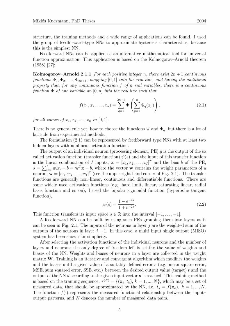
The output of an individual neuron (processing element, PE) y is the output of the socalled activation function (transfer function) ψ(s) and the input of this transfer functionis the linear combination of I inputs, x = [x1, x2, . . . , xI ]
T and the bias b of the PE,s =
∑Ii=1 wixi + b = wTx + b, where the vector w contains the weight parameters of a
neuron, w = [w1, w2, . . . , wI ]T (see the upper right hand corner of Fig. 2.1). The transfer
functions are generally non–linear, continuous and differentiable functions. There aresome widely used activation functions (e.g. hard limit, linear, saturating linear, radialbasis function and so on), I used the bipolar sigmoidal function (hyperbolic tangentfunction),
ψ(s) =1− e−2s
1 + e−2s. (2.2)
This function transfers its input space s ∈ R into the interval [−1, . . . ,+1].A feedforward NN can be built by using such PEs grouping them into layers as it
can be seen in Fig. 2.1. The inputs of the neurons in layer j are the weighted sum of theoutputs of the neurons in layer j − 1. In this case, a multi input single output (MISO)system has been shown for simplicity.
After selecting the activation functions of the individual neurons and the number oflayers and neurons, the only degree of freedom left is setting the value of weights andbiases of the NN. Weights and biases of neurons in a layer are collected in the weightmatrix W. Training is an iterative and convergent algorithm which modifies the weightsand the biases until a given value of a suitably defined error ε (e.g. mean square error,MSE, sum squared error, SSE, etc.) between the desired output value (target) t and theoutput of the NN d according to the given input vector x is reached. This training methodis based on the training sequence, τ (N) = (xk, tk), k = 1, ..., N, which may be a set ofmeasured data, that should be approximated by the NN, i.e. tk = f(xk), k = 1, ..., N .The function f(·) represents the measured functional relationship between the input–output patterns, and N denotes the number of measured data pairs.
5
Miklos Kuczmann, PhD Theses 2004
PSfrag replacements
Training algorithm
x1
x1
x2
x2
x3
xI
xI
input layer hidden layers
W(1)
W(i)
W(L)
4W
w
... ...
. . .
...
...
t
d
λ
b
y
output
P
Pψ
+–
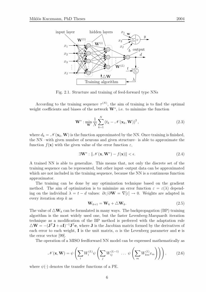
Fig. 2.1. Structure and training of feed-forward type NNs
According to the training sequence τ (N), the aim of training is to find the optimalweight coefficients and biases of the network W∗, i.e. to minimize the function
W∗ : minW
1
N
N∑
k=1
(tk −N (xk,W))2 , (2.3)
where dk = N (xk,W) is the function approximated by the NN. Once training is finished,the NN –with given number of neurons and given structure– is able to approximate thefunction f(x) with the given value of the error function ε,
∃W∗ : ‖N (x,W∗)− f(x)‖ < ε. (2.4)
A trained NN is able to generalize. This means that, not only the discrete set of thetraining sequence can be represented, but other input–output data can be approximatedwhich are not included in the training sequence, because the NN is a continuous functionapproximator.
The training can be done by any optimization technique based on the gradientmethod. The aim of optimization is to minimize an error function ε = ε(λ) depend-ing on the individual λ = t − d values: ∂ε/∂W = ∇[ε] → 0. Weights are adapted inevery iteration step k as
Wk+1 = Wk +4Wk. (2.5)
The value of4Wk can be formulated in many ways. The backpropagation (BP) trainingalgorithm is the most widely used one, but the faster Levenberg-Marquardt iterationtechnique as a modification of the BP method is preferred with the adaptation rule4W = −(JTJ +αI)−1JTe, where J is the Jacobian matrix formed by the derivatives ofeach error to each weight, I is the unit matrix, α is the Levenberg parameter and e isthe error vector [99].
The operation of a MISO feedforward NN model can be expressed mathematically as
N (x,W) = ψ
(∑
i
W(L)i ψ
(∑
j
W(L−1)ij . . . ψ
(∑
m
W(1)kmxm
))), (2.6)
where ψ(·) denotes the transfer functions of a PE.
6
Miklos Kuczmann, PhD Theses 2004
Using the chain rule, the derivatives of the formulation (2.6) with respect to anyinput of the NN can be expressed in analytical form.
This is the general form of feedforward type NNs; although not all models share allof the characteristics. Individual neurons can have numerous inputs and can send datato numerous other PEs. There is such a large variety of NNs.
2.2 Preisach–type hysteresis models based on NN
The hysteresis phenomenon is encountered in many different areas of science, and hasbeen in the focus of research and investigation for a long time. Thanks to the fastcomputers available nowadays, it is possible to simulate hysteresis characteristics moreand more precisely taking into account important physical phenomena. The developedmodels can be inserted into field calculation software to examine an investigated materialor an arrangement.
There are many hysteresis models to simulate the behavior of magnetic materials,such as the Preisach model [39, 67, 88, 93], the Jiles–Atherton model [43], the Stoner–Wohlfarth model [18,39,88,93] etc., and applying a new technique, the method of NNs,which will be presented with references in this section.
The investigated NN model of magnetic hysteresis presented in this dissertation ismainly based on the ideas of the Preisach model, therefore this model with its modifi-cations, and some methods, where the NN techniques are used are briefly described andoverviewed.
2.2.1 The classical scalar Preisach model
The classical scalar Preisach model [31, 32, 39, 67, 88, 93] describes the scalar hysteresisphenomenon as a collection of elementary shifted rectangular hysteresis operators γ(α, β)with different coercive fields (see Fig. 2.2). The switching fields α and β –where themagnetization jumps up from −1 to +1 and jumps down from +1 to −1, respectively–characterize each operator. The operators also can be defined by their coercive field,hc = (α − β)/2 and their interaction field, hm = (α + β)/2. The magnetization M canbe expressed by the integral
M(t) =
∫∫
α≥β
µ(α, β) γ(α, β)H(t) dαdβ, (2.7)
where µ(α, β) is the Preisach distribution function, i.e. the weight function of the ele-mentary hysteresis operators γ(α, β), H(t) is the applied magnetic field intensity, andM(t) is the magnetization at time t. In a computer realization, the integral (2.7) isapproximated by the weighted sum of elementary operators as
M(t) 'N+1∑
i=1
N+1∑
j=N+2−i
µ(αi, βj) γ(αi, βj)H(t), (2.8)
where N is the number of subdivisions in the Preisach plane. Each point on the halfspace α ≥ β corresponds to one elementary hysteresis operator only. In this way, a math-ematical representation can be introduced and known as the Preisach triangle [39, 67],
7

Miklos Kuczmann, PhD Theses 2004
PSfrag replacements
αβ
+1
-1hm
hc hc
H
M
Fig. 2.2. Magnetization curve of an elementary hysteresis operator, γ(α, β)
PSfrag replacements
α
β
+1
+1
-1
-1
α=β
hm
hc
L(t)
i
j
bγ = +1
bγ = −1
Fig. 2.3. The Preisach triangle and the staircase line
shown in Fig. 2.3. Applying the staircase line L(t), the magnetization can be calcu-lated taking into account the prehistory of the material. Increasing the magnetic fieldintensity, the staircase line is moving from left to right, and decreasing the magneticfield intensity, the staircase line is moving from top to bottom on the Preisach triangleswitching the elementary operators, and the magnetization can be calculated by the for-mula (2.8). The Preisach distribution function can be easily approximated by Gaussianor exponential distribution functions, and the parameters of these distributions can befitted to experimentally measured hysteresis curves.
Using the Everett function leads to a very favorable implementation of the Preisachmodel [39, 67]. The discrete Everett table must be calculated once from the measuredfirst order reversal curves at very low frequency (f < 1 Hz), avoiding the computationof the integral in (2.7) or the sum in (2.8). It gives a better approximation, because theEverett function is very close to measurements,
E(α, β) =1
2(Mα −Mα,β), (2.9)
where Mα is a reversal magnetization point in the major hysteresis loop corresponding tothe magnetic field intensity α, and Mα,β is the value of magnetization in a reversal curvestarting from the reversal point (α,Mα), when the magnetic field intensity is equal toβ. A reversal curve with given points can be seen in Fig. 2.4. The Preisach distribution
8

Miklos Kuczmann, PhD Theses 2004
−1 −0.5 0 0.5 1−1
−0.5
0
0.5
1
H/Hs
M/M
s
α β
Mα
Mα,β
Fig. 2.4. A first order reversal curve to measure the Everett function
−1
−0.5
0
0.5
1
−1
−0.5
0
0.5
10
0.25
0.5
0.75
1
αβ
E(α
,β)
(a) The Everett function
−1
−0.5
0
0.5
1
−1
−0.5
0
0.5
10
0.25
0.5
0.75
1
αβ
µ(α,
β)
(b) The Preisach distribution func-tion
Fig. 2.5. The Everett function and the Preisach distribution function
function can be expressed from the Everett function as
µ(α, β) =∂2E(α, β)
∂α ∂β, and E(α, β) =
∫∫
α≥β
µ(α′, β ′) dα′ dβ ′. (2.10)
The differentiation must be performed numerically from the measured Everett functionwhich amplifies the measurement noise. An example –generated by the Preisach model–for a calculated Everett function E(α, β) and the corresponding distribution functionµ(α, β) are plotted in Fig. 2.5(a) and in Fig. 2.5(b), respectively.
Knowing the Everett function, the following expression can be used to determine the
9

Miklos Kuczmann, PhD Theses 2004
magnetization [67, 72]:
M = −E(α0, β0) + 2
n∑
k=1
E(Mk, mk−1)− E(Mk, mk) , (2.11)
where Mknk=1 and mk
nk=1 are the increasing and the decreasing sequences of the
magnetic field intensity applied to the sample and stored by using the staircase line, andα0 = 1, β0 = −1.
The classical scalar Preisach model is unable to describe some phenomena, such asnoncongruency [39, 44, 67] and accommodation [39, 67, 94]. Simulated minor loops arecongruent, i.e. a stable minor loop cycling between two fixed values of the applied fieldhas the same size and shape. The moving model [39, 72] and the product model [39, 45]can solve this problem. The moving model contains the classical Preisach model witha feedback which modifies the actual value of the applied magnetic field intensity bya term of αM , i.e. Hk = Hk + αMk−1 at the discrete time of simulation tk, and α isa small positive number. In the product model, the rate of change of magnetizationwith respect to the applied field dM/dH is expressed by a Preisach–like integral formulamultiplied by a function R(M). Accommodation of a loop means that, it takes manycycles for a minor hysteresis loop to stabilize and it continues until an equilibrium isreached asymptotically. The moving model and the product model also can fulfill thisproperty. Accommodation cannot be simulated by the classical Preisach model, becausea minor loop closes at the same point (H,M), where it was started. This is caused bythe wiping–out property.
2.2.2 The classical scalar Preisach model via NNs
The memory storage mechanism of the ferromagnetic materials can be described bymeans of the Preisach triangle. Several papers have been written about this approachwhen using NNs.
The authors of [84] used a discrete set of Play operators Ψj = Ψ(t, hjc), j = 0, ..., J−1to simulate the memory mechanism of magnetic materials and a feedforward NN tostore the experimentally measured data set B = HBΨ(t, hjc). The block diagram ofthis model can be seen in Fig. 2.6. The authors have considered a NN with J = 20inputs and one hidden layer with 40 neurons. Each neuron employs a bipolar sigmoidalactivation function. The training data set has contained 50 H−B pairs in a nested loop.Five first order reversal curves have been measured in one magnetic sample and sevenin another sample. They have demonstrated the good quality of the predictions of themodel by comparing simulation results and measured symmetrical minor loops. Thismodel has also been applied to simulate noisy and incomplete measurement data [98].It is very difficult to identify the classical Preisach model when the reversal curves havebeen loaded with noise, but NNs are able to filter the noise during the learning process.Preprocessing of noisy measured data is not required in this case.
A possible way to represent the main features of the classical scalar Preisach modelapplying NNs can be found in [1]. The block representation of the Preisach modelhas been realized by a NN structure with bipolar sigmoidal activation function, if thehysteresis operators are represented by elementary rectangular loops γ(α, β), and thedistribution function µ(α, β) has been characterized by the weights of the network asillustrated in Fig. 2.7. This means that, a large number of inputs (few hundred), and
10

Miklos Kuczmann, PhD Theses 2004
PSfrag replacements
H B
α
β
hc hm Ψ0
ΨJ−1
Ψj
......
discrete set of Play operators neural network
Fig. 2.6. Implementation via feedforward NN of the system with Preisach memory
PSfrag replacements H B
NN
hysteresis operators
...
......
Fig. 2.7. Operator NN realization of the classical Preisach model
consequently a large number of unknown weights are required for the model, so theauthors have grouped the rectangular operators into a smaller, but more sophisticatedset of 20 hysteresis operators having different widths and 10 neurons in one hidden layer.The measured data set contains 304 H −B pairs in the form of a decreasing oscillatingsequence. After training, higher order minor loops are demonstrated and compared withmeasured data.
The approximation of the Preisach distribution function or the Everett function canbe realized by a feedforward NN with 2 inputs (α and β) and one output (µ(α, β)or E(α, β)) [23]. The output of a NN having continuous and differentiable activationfunctions can be differentiated with respect to its input, and the value of the differentialsusceptibility χdiff = dM/dH is a continuous function of H and it can be expressedin analytical form. Applying the Newton–Raphson iteration technique in numericalfield calculation problems leads to faster convergence, but this technique requires thedifferential susceptibility. It is also shown in the paper that, the integral form (2.7), aswell as the energy losses can also be worked out by an analytical expression when NNsare used. It gives a computationally effective model. The authors used a NN with 75neurons in one hidden layer to approximate a measured Everett surface with very goodaccuracy.
NN technique combined with the Fourier description can be used to calculate themagnetization in cases when a periodic magnetic field excites the ferromagnetic device aspresented in [80]. This method is a quite simple computational instrument for designersand takes into account the frequency dependence of the hysteresis characteristics.
A nonlinear circuit model of hysteresis characteristics can be developed as proposedin [20]. The investigated model is based on a two–layer feedforward connected nonlinearcircuit. The first layer contains elementary cells (simple hysteresis operators) and thesecond layer is a simple adder. The parameter identification of this model can be solved
11

Miklos Kuczmann, PhD Theses 2004
by a NN approach. The proposed model has been compared with the Jiles–Athertonhysteresis model and a good agreement has been found, including the dynamic properties(e.g. frequency dependence) of the hysteresis loop.
The dynamic Preisach model which encompass the dynamic effects such as the eddycurrents and the domain wall displacement is a generalization of the static Preisachmodel introducing the rate of change of the magnetization dM/dt [30, 39, 67], i.e.
M(t) =
∫∫
α≥β
µ(α, β, dM/dt) γ(α, β)H(t) dαdβ. (2.12)
The rate dependent generalization of the Preisach model considers the hysteresis switchesto be not ideal ones [5], but their output changes at a finite rate, so ideal rectangularhysterons are changed to idealized magnetization characteristic. The disadvantage ofthis model is the time consuming calculation of the output.
This effect can also be handled by the classical Preisach model coupled with a differ-ential equation as shown in [30]. The differential equation responsible for the dynamicfeatures uses a variable Hm as input for the static Preisach model delayed with respectto the actual field strength H is
dHm
dt= a(H −Hm)− b
dB
dt+ c
dH
dt, (2.13)
where dH/dt and dB/dt are the magnetic field intensity and the magnetic flux densityvariation rates and a, b and c are model parameters, adjusted by an iterative method.
A recurrent NN can be used to handle time dependent mapping. The authors of [79]used the Elman type recurrent NN which is a three–layer recurrent network. The middlelayer is recurrent containing hidden and context neurons. The context neurons act asa delay in one sampling period, meaning that, the magnetization is a function of thepresent state, the previous state and the present magnetic field intensity. The networkwas trained using two symmetrical hysteresis loops and tested with another loop differentfrom the training sequence. The simulation results agree well with the experimentalmeasurements, but minor loops are not shown in the paper.
I have developed a new NN based hysteresis operator which differs from the abovemodels (Chapter 3). Measured curves are approximated by NNs, the memory mechanismof the model is based on a knowledge–base containing the properties of the hysteresischaracteristics as if–then rules.
2.2.3 Vector hysteresis modeling
Scalar hysteresis characteristics can simulate special cases, when the magnetic field in-tensity and the magnetization vectors are in the same direction (e.g. inside a toroidalshape core), but generally, these vectors do not have the same directions. In this case, avector hysteresis model must be used.
The Stoner–Wohlfarth model is the most successful physics–based model, because agraphical representation by means of an astroid can be used to follow the magnetizationvector in the presence of a two–dimensional magnetic field intensity [5, 39, 88, 93]. Theanisotropic behavior is embedded in the equations of the model, but the identificationprocess is a difficult task.
12
Miklos Kuczmann, PhD Theses 2004
The most widely used vector model is proposed by Mayergoyz [67]. This is an exten-sion of the classical Preisach model, because this vector model is built as a superpositionof continuously distributed scalar Preisach models in given directions eϕ of the 2D plane.The magnetization vector M can be expressed in two dimensions as
M =
∫ π/2
−π/2
eϕ H Hϕ dϕ, (2.14)
where Mϕ = H Hϕ is the scalar magnetization in the direction eϕ. The character-istic H · depends on the polar angle ϕ if the magnetic material presents anisotropy,otherwise it is ϕ–independent [10, 67, 77, 78].
The identification process can be worked out by applying either the Everett func-tion or the Preisach distribution function both for isotropic and anisotropic case. Theidentification process is based on the integral equation
F (α, β) =
∫ π/2
−π/2
cosϕE(α cosϕ, β cosϕ) dϕ, (2.15)
where F (α, β) and E(α, β) are the measured scalar Everett function and the unknownvector Everett function. The identification process based on the Preisach distributionfunction can also be applied, i.e.
µ(α, β) =
∫ π/2
−π/2
cos3 ϕ ν(α cosϕ, β cosϕ) dϕ, (2.16)
where µ(α, β) and ν(α, β) are the measured scalar distribution function and the unknownvector distribution function. These integral equations can be solved only numerically,because no analytical solution is available, that is why the Preisach triangle must bedivided into elements.
The above integral equations are valid for isotropic characterization for simplicity.A possible solution composed with the Preisach distribution function of an anisotropicmaterial with the help of Fourier expansion can be found in [78].
Working out a vector hysteresis measurement system is an extensive project [34,64,85,86], therefore, it is sometimes simpler to use a known model to generate measurements.
A vectorial realization based on NN technique has been investigated and performedin [2]. After some mathematical formulations of the basic equations of the anisotropic2D vector Preisach model and applying Fourier expansion, the vector Preisach modelcan be identified by a two layer feedforward type NN. The input layer consists of twiceas many nodes as the number of elementary hysteresis operators necessary to constructa reasonably accurate hysteresis model. Only 36 rectangular elementary hysteresis op-erators have been used in the model. The identification of the model is based on 706H −M pairs. Measured first order reversal curves have been compared with predictionsof the model.
I have worked out an original identification method based on the measured Everettfunction to simulate both isotropic and anisotropic magnetic materials. A possible gen-eralization for 3D also will be presented in Chapter 3, however, only two–dimensionalanisotropic vector models are known from the literature.
13

Miklos Kuczmann, PhD Theses 2004
2.3 The nondestructive testing method
Structural damage may result from a number of causes and it can be of different types. Itis most often called crack which is a change in the geometry with respect to the uncrackedstate of the structure. Early stages of cracks may be undetectable, but cracks maygrow and propagate at a very high rate quickly compromising the structural integrity.Detection of cracks is the main goal of the damage detection systems under design [46,81].
There are two main groups of testing of materials in the industry, destructive andnondestructive testing methods.
In the first case, a sample from the analyzed structure must be taken and examined ina laboratory. After making a standardized test specimen (with given size and shape) fromthe sample, some measurements can be done, such as the hardness test, the Charpy’sstriking–bending test, tensile strength test, measuring different electrical properties andso on [76].
In nondestructive testing (NDT), the tested material is not damaged [46, 81], but itneeds more precise measuring equipments controlled by computers. Thanks to the intenseadvance in computer techniques, these methods have an extreme advance nowadaysresearched by many engineers. Using computers and electronic control in NDT systemsallows to reduce operator workload and improves the speed and quality of the process.Of course, it requires extensive software development, too. The reason for this extensivework is that, products of standardized production must satisfy increasingly rigorouscriteria. Monitoring can be worked out by fast and precise measuring arrangements. Theautomation of NDT techniques and procedures is beginning to spread among differentindustries and fields of engineering. The benefits of automated NDT include more reliableand more predictable operation machinery, decreased probability of industrial accidentsand less operation costs.
There are several major directions of such methods. For example the X–ray method isthe first flaw detection technique, the UV optical technique with digital image processingmethods, measuring with electronmicroscope, the ultrasonic test [95]. I mainly focuson the magnetic flux leakage method [46]. In short, the basis of the magnetic fluxleakage method is that, inhomogenities (like cracks, slots and flaws) change the generatedhomogeneous field distribution inside the material, and this field perturbation can bemeasured by an appropriate sensor. The specimen can be magnetized either by passinga direct current throught it or by applying an external magnetic field. It is easy tounderstand that, the surface cracks can be identified much easier than cracks lyinginside the material, because flux lines disperse to the area surrounding the defect, butthis problem can be handled by choosing an appropriate frequency or amplitude of theexcitation. It is also hard to find a crack parallel to the magnetic flux. Much betterresults can be obtained when two separate and perpendicular magnetization fields areused, because cracks with any orientation can be detected then.
The other general magnetization process found in the literature is to move an ex-citing coil above the specimen generating a magnetic field intensity. The leakage fieldmodified by the eddy currents inside the material can be measured then. This methodis limited by the skin effect only to thin and non–magnetic structural components. Apossible alternative is the use of pulse eddy currents [12,15,74], when the rich harmoniccomponent of a pulse accounts for a multi–frequency analysis, since the lower harmonicspenetrating deeper into the structure.
14

Miklos Kuczmann, PhD Theses 2004
An increasing number of articles about nondestructive testing (e.g. [13, 14, 28, 37,71, 74, 95, 96] and so on) can be found in books, proceedings and journals in recentyears. There are many sensors [15, 28, 33, 37, 69–71, 75, 96, 97], measuring arrangementsand visualization techniques described in the literature. There are two main groupsof probes: measuring the changes in coil impedance, and measuring induced voltages.The measuring test arrangement consists of a test specimen with artificial cracks, apositioning device which is used to scan the surface by moving the probe above the testspecimen and a computer to control the measuring system and to store the measureddata.
The applied simulation techniques are mainly based on the finite element method withdifferent potential formulations. Modeling natural cracks is a long–standing and difficulttask, let us think about pits caused by corrosion, hairline cracks with varying shapeand depth, flaws and so on [89]. Such natural cracks can be found in real industrialenvironment. It is in the scope of interest of many projects to form the complicatedprofiles of natural cracks, but in computation it is obvious to use simply characterizedcracks of elliptical, semielliptical or rectangular shape. The simplest model is to discretizethe geometry by finite elements and to assign the same material properties to crack asto the air region.
Visualization, as well as recognition and identification of damage are also impor-tant stages in NDT techniques [3,14,69,70,74,92,103,104]. The recognition is an inverseproblem. It should be performed automatically with high reliability. In the field of recog-nition and classification of computational intelligence (as fuzzy systems, neural networks,neuro–fuzzy systems, knowledge–based systems) there is an increasing challenge and re-vival of learning. It is the main direction of research which replaces the statistical andtraditional methods.
A search of literature (IEEE Transactions on Magnetics, Electromagnetic Nonde-structive Evaluation, Applied Electromagnetics and Mechanics in the frame of Studiesin Applied Electromagnetics and Mechanics, and Proceedings of Conferences) show awide and increasing area of automated NDT applications. There are several benchmarkproblems aimed at working out the common standards and solvers, to compare differentnumerical techniques. This activity shows the increasing importance of this field.
2.4 Formulation and potentials of the electromag-
netic field problems
An electromagnetic field calculation problem can be characterized by the field intensitiesand the flux densities described by partial differential equations derived from Maxwell’sequations and boundary conditions [6, 21, 29, 40, 41, 87]. There are several potentialformulations applicable to calculate the field quantities, fundamentally using scalar andvector potentials. In this section, I briefly overview only the most popular formulationsused in the simulation of nondestructive testing methods in connection with the FiniteElement Method (FEM) [6,7,16,68,90,91], especially with the edge element based FEM.Essentially, NDT represents an eddy current field problem.
At low frequencies and with normal conducting materials used in NDT techniques,the displacement currents are small compared with the conductive currents and canbe neglected. Consequently, the studied electromagnetic field can be described by the
15
Miklos Kuczmann, PhD Theses 2004PSfrag replacements
i(t)
conducting region
nonconducting region
µ0
H ·σ
Ωc
Ωn
Γnc
Γn
Γccrack
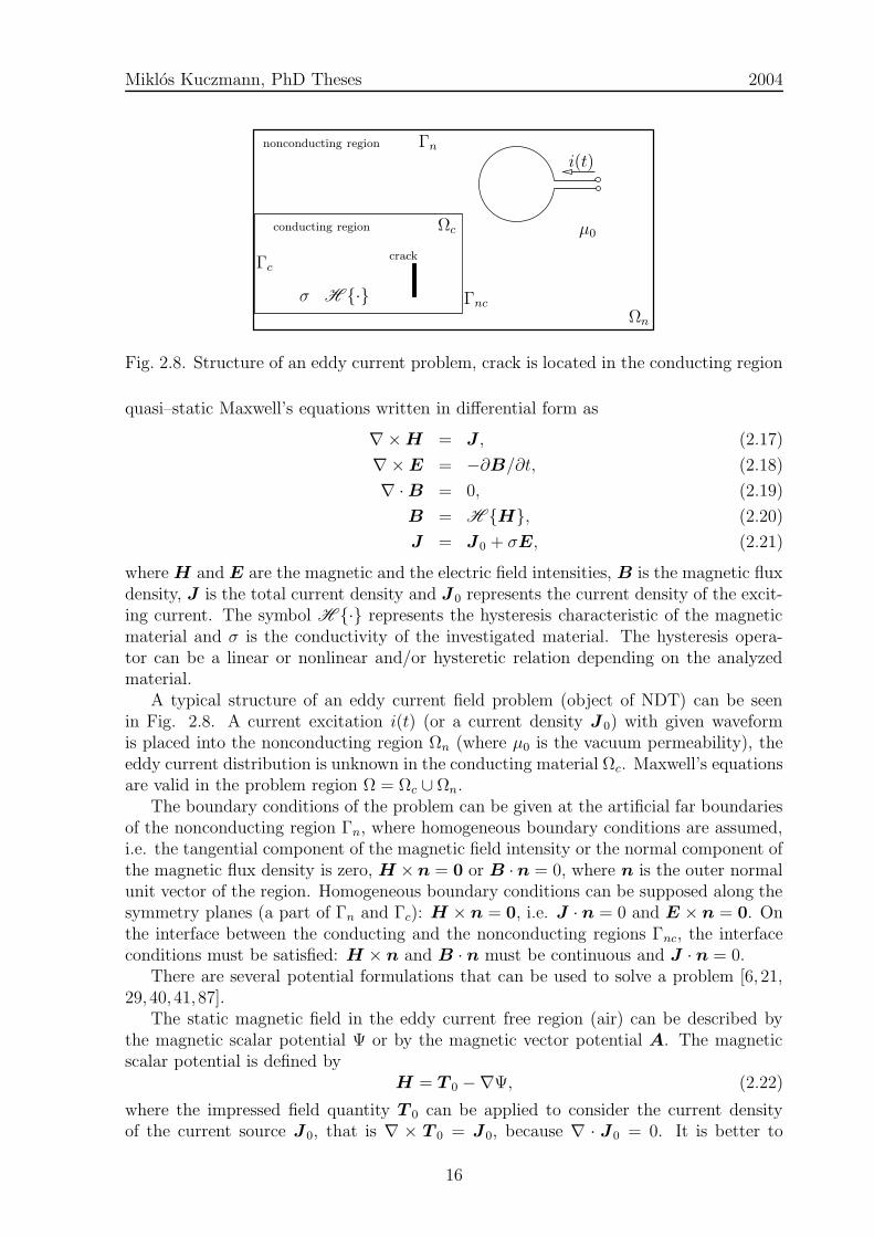
Fig. 2.8. Structure of an eddy current problem, crack is located in the conducting region
quasi–static Maxwell’s equations written in differential form as
∇×H = J , (2.17)
∇×E = −∂B/∂t, (2.18)
∇ ·B = 0, (2.19)
B = H H, (2.20)
J = J0 + σE, (2.21)
where H and E are the magnetic and the electric field intensities, B is the magnetic fluxdensity, J is the total current density and J 0 represents the current density of the excit-ing current. The symbol H · represents the hysteresis characteristic of the magneticmaterial and σ is the conductivity of the investigated material. The hysteresis opera-tor can be a linear or nonlinear and/or hysteretic relation depending on the analyzedmaterial.
A typical structure of an eddy current field problem (object of NDT) can be seenin Fig. 2.8. A current excitation i(t) (or a current density J 0) with given waveformis placed into the nonconducting region Ωn (where µ0 is the vacuum permeability), theeddy current distribution is unknown in the conducting material Ωc. Maxwell’s equationsare valid in the problem region Ω = Ωc ∪ Ωn.
The boundary conditions of the problem can be given at the artificial far boundariesof the nonconducting region Γn, where homogeneous boundary conditions are assumed,i.e. the tangential component of the magnetic field intensity or the normal component ofthe magnetic flux density is zero, H ×n = 0 or B ·n = 0, where n is the outer normalunit vector of the region. Homogeneous boundary conditions can be supposed along thesymmetry planes (a part of Γn and Γc): H × n = 0, i.e. J · n = 0 and E × n = 0. Onthe interface between the conducting and the nonconducting regions Γnc, the interfaceconditions must be satisfied: H × n and B · n must be continuous and J · n = 0.
There are several potential formulations that can be used to solve a problem [6, 21,29, 40, 41, 87].
The static magnetic field in the eddy current free region (air) can be described bythe magnetic scalar potential Ψ or by the magnetic vector potential A. The magneticscalar potential is defined by
H = T 0 −∇Ψ, (2.22)
where the impressed field quantity T 0 can be applied to consider the current densityof the current source J 0, that is ∇ × T 0 = J0, because ∇ · J0 = 0. It is better to
16
Miklos Kuczmann, PhD Theses 2004
find an approximating vector potential T 0 to take into account the effect of the excitingcurrent, than generating a mesh for J 0, since it leads to a consistent right hand side ofthe equations, moreover the exact modeling of the coils can be avoided. The magneticscalar potential is approximated by nodal shape functions, T 0 can be represented by theaid of edge basis functions.
The magnetic vector potential is defined by
B = ∇×A (2.23)
which satisfies (2.19) exactly. The magnetic vector potential can be approximated bynodal or edge shape functions as well, depending on the dimension of the problem.The reduced vector potential Ar, approximated by edge shape functions can be appliedmore efficiently if current sources are present, since the right hand side of the assembledequation is then consistent. The reduced vector potential can be introduced as
B = µ0Hs +∇×Ar, (2.24)
where Hs is the Biot–Savart field of the exciting current flowing in the exciting coils.The use of the magnetic scalar potential in eddy current free region reduces the
computational costs as compared with the use of the magnetic vector potential, becauseΨ has only one component, and A has three components, when using nodal shapefunctions. Furthermore, the use of A requires the inclusion of the coils in the meshincreasing the number of unknowns. A simpler mesh can be generated by using thevector field of T 0.
Two potential functions can be used in the eddy current region, either a current vectorpotential T or a magnetic vector potential A. The current vector potential approximatedby edge shape functions can be applied more effectively when thin flaws in the conductingmaterial are present [7]. The current vector potential is introduced as [6]
H = T 0 + T −∇Ψ. (2.25)
The magnetic vector potential can be applied in several ways: the A∗–formulation,
the A, V –formulation, and the Ar, V –formulation and some other combinations of thepotentials as presented in [6].
The various formulations in the conducting and nonconducting regions must be cou-pled through the interface conditions. In my research work, I used the T ,Ψ − Ψ for-mulation. In this case, Ψ is approximated by nodal shape functions, T and T 0 areapproximated by edges shape functions, Ψ and T 0 are defined in the whole region Ω,and T is defined only in the conducting region Ωc.
2.5 The finite element method
By using potentials, Maxwell’s equations can be transformed into partial differentialequations and they can be solved by numerical methods. The basis of numerical tech-niques is to reduce the partial differential equations to algebraic equations whose solutiongives the unknown potentials in the given points of a mesh. This reduction can be done bydiscretizing the partial differential equations in time and in space as well. The potentialfunctions, the approximation method and the generated mesh distinguish the numerical
17
Miklos Kuczmann, PhD Theses 2004
field solvers. There is a number of methods, e.g. the finite element method, the finitedifference method, the boundary element method, the integral equation method and theglobal variational method [40, 41].
The FEM is the most popular and flexible numerical technique to determine theapproximate solution of partial differential equations in engineering [8, 21, 35, 82, 105].The fundamental idea of the FEM is to divide the problem region to be analyzed intosmaller finite elements with given shape (e.g. triangles in 2D or tetrahedra in 3D). Thescalar potential functions can be approximated by nodal shape functions, and the vectorpotential functions can be approximated by either nodal or vector shape functions. Ashape function is a simple continuous polynomial function defined in a finite element.Applying first–order nodal and edge shape functions, the unknown potentials can beassociated with the nodes as well as the edges of the finite element mesh. Shape functionsare described below in this section.
The finite element analysis consists of four main steps. The first step is to workout a simplified mathematical model of the arrangement which is adequate to calculateelectromagnetic field quantities. There may be some details that can be neglected orsimplified, e.g. the symmetry of the equipment can be taken into account. This cannotbe automated, it is advisable to build a problem specific model. The preprocessingtask is the second step when the geometry, the material parameters, the excitationwaveform, etc. must be given and then the finite element mesh can be generated. Thenext step is the calculation, generation of the element based equations, assembling ofthe global system of linear equations, and the solution of the assembled equations mustbe performed. The last step is the postprocessing, when calculated results are plottedand shown, quantities of interest (e.g. capacity, losses) are calculated. There are somefeedbacks during FEM calculations, for example to make a denser mesh, to vary timesteps and so on. If the problem to be solved is nonlinear, then an iterative feedback mustbe used during the third step of calculations.
In my research, I used the first–order nodal and edge shape functions which varylinearly in a finite element to determine the magnetic field intensity above a test specimenwith well defined surface cracks (slots and holes with different, but well defined size). Aproblem not easily treated by nodal finite elements arises, when singularities are to beapproximated at sharp corners, for example at cracks in a conducting material. This isthe reason why I used the combined nodal and edge finite elements.
My work is mainly based on the papers [6, 36, 66] and on the dissertation [21]. Inthe followings, I briefly describe the nodal and edge finite elements, following the aboveliterature.
2.5.1 Nodal finite elements
Scalar potential functions can be represented by a linear combination of shape functionsassociated with nodes of the finite element mesh. Within a finite element, a scalarpotential function Ψ = Ψ(r, t) is approximated by Ψh = Ψh(r, t) as
Ψh '
I∑
i=1
NiΨi, (2.26)
where Ni = Ni(r) and Ψi = Ψi(t) are the first–order nodal shape functions and the valueof potential function corresponding to the ith node. The number of degrees of freedom
18

Miklos Kuczmann, PhD Theses 2004
is I = 3 in a 2D problem using triangular FEM mesh and I = 4 in a 3D arrangementmeshed by tetrahedral elements.
The sum of all nodal shape functions is equal to 1,∑I
i=1Ni = 1, hence the sum of
their gradients is zero,∑I
i=1∇Ni = 0. This means that, the maximal number of linearlyindependent gradients of the nodal basis functions is I − 1. The shape functions arepresented in the sections 2.5.3 and 2.5.4.
2.5.2 Edge finite elements
Vector potentials can be represented by nodal shape functions as well. The naturalapproach is to treat the vector field T = T (r, t) as two (in 2D) or three (in 3D) coupledscalar fields, Tx, Ty and Tz. Scalar shape functions can be used again, i.e. each node hastwo (2D) or three (3D) unknowns, and scalar shape functions can be used. For examplein 3D, T can be approximated by T h = T h(r, t) as
T h '
I∑
i=1
(Tx,iex + Ty,iey + Tz,iez)Ni. (2.27)
Instead of scalar shape functions, I used vector shape functions
T h 'K∑
k=1
W k Tk, (2.28)
where W k = W k(r) and Tk = Tk(t) are the first–order edge shape functions and thedegree of freedom is associated to the edges. The number of degrees of freedom is K = 3in 2D when applying triangular mesh and K = 6 in the 3D case by applying tetrahedralfinite elements. The shape functions are also presented in the sections 2.5.3 and 2.5.4.
I used linear elements [21], having only K unknowns in each finite element, oneattached to each edge. They allow the normal component of the field to be free to jumpat each facet of the element. The direction of the edges must be defined by the globalmesh, but the equations of one element assume a local orientation.
The line integral of the shape functions W k along the kth edge is equal to one,meaning that the line integral of the vector potential along this edge is Tk,
∫
lk
T h · dl =
∫
lk
(W kTk) · dl = Tk. (2.29)
This means that, the value of Tk along an edge of a finite element is equal to the valueof Tk along the edge of another finite element if these finite elements share the edge.Therefore the vector function T is tangentially continuous across all element interfaces,but its normal component is not.
The gradients of the nodal shape functions are in the function space spanned by theedge basis functions, that is
∇Ni =K∑
k=1
cikW k, i = 1, . . . , I − 1, (2.30)
19
Miklos Kuczmann, PhD Theses 2004
where∑K
k=1 c2ik > 0. Taking the curl of each equation in (2.30) results in
K∑
k=1
cik∇×W k = 0, i = 1, . . . , I − 1. (2.31)
This shows that, the maximal number of linearly independent curls of the edge basisfunctions is K − (I − 1). The interdependence of the curls of the edge basis functionsmeans that, an ungauged formulation leads to a singular, positive semidefinit finiteelement curl–curl matrix. Singular systems can be solved by iterative methods, if theright hand side of the system of equations is consistent.
2.5.3 FEM in 2D using linear shape functions
I used a finite element mesh with triangular finite elements. Linear basis functions canbe introduced by using the barycentric coordinate system in a finite element. The areaof a triangle is denoted by 4, and it can be calculated as
4 =1
2
∣∣∣∣∣∣
1 x1 y1
1 x2 y2
1 x3 y3
∣∣∣∣∣∣,
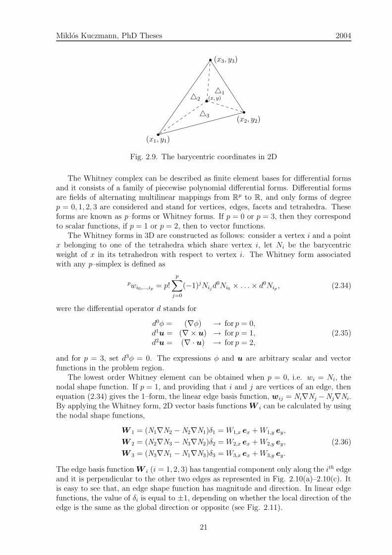
where (x1, y1), (x2, y2) and (x3, y3) are the coordinates of the three nodes of the trianglein the global coordinate system building an anticlockwise sequence. The area functions(see Fig. 2.9) of a given point inside the triangle with coordinates (x, y) can be calculatedas
41 =1
2
∣∣∣∣∣∣
1 x y1 x2 y2
1 x3 y3
∣∣∣∣∣∣, 42 =
1
2
∣∣∣∣∣∣
1 x1 y1
1 x y1 x3 y3
∣∣∣∣∣∣, 43 =
1
2
∣∣∣∣∣∣
1 x1 y1
1 x2 y2
1 x y
∣∣∣∣∣∣.
Three linear shape functions Ni can be described by the above area functions as
Ni = 4i/4, i = 1, 2, 3. (2.32)
A shape function Ni is equal to 1 at the ith node of the triangle, and equal to zero atthe other two nodes and varies linearly over the triangle. If the potentials at the nodesare known, then a linear approximation of the potential function can be represented by(2.26).
The gradients of the basis functions are used to assemble the global system of equa-tions, and the constant gradients of linear shape functions can be calculated as
∇N1 =(y2 − y3) ex + (x3 − x2) ey
/ 24,
∇N2 =(y3 − y1) ex + (x1 − x3) ey
/ 24,
∇N3 =(y1 − y2) ex + (x2 − x1) ey
/ 24.
(2.33)
Whitney complex
The first–order (linear) edge basis functions can be generated by means of the Whitneycomplex, briefly described here, the extensive mathematical background can be foundin [9, 21].
20
Miklos Kuczmann, PhD Theses 2004
PSfrag replacements
(x1, y1)
(x2, y2)
(x3, y3)
41
43
42 (x, y)
Fig. 2.9. The barycentric coordinates in 2D
The Whitney complex can be described as finite element bases for differential formsand it consists of a family of piecewise polynomial differential forms. Differential formsare fields of alternating multilinear mappings from R
p to R, and only forms of degreep = 0, 1, 2, 3 are considered and stand for vertices, edges, facets and tetrahedra. Theseforms are known as p–forms or Whitney forms. If p = 0 or p = 3, then they correspondto scalar functions, if p = 1 or p = 2, then to vector functions.
The Whitney forms in 3D are constructed as follows: consider a vertex i and a pointx belonging to one of the tetrahedra which share vertex i, let Ni be the barycentricweight of x in its tetrahedron with respect to vertex i. The Whitney form associatedwith any p–simplex is defined as
pwi0,...,ip = p!
p∑
j=0
(−1)jNijd0Ni0 × . . .× d
0Nip , (2.34)
were the differential operator d stands for
d0φ = (∇φ) → for p = 0,d1
u = (∇× u) → for p = 1,d2u = (∇ · u) → for p = 2,
(2.35)
and for p = 3, set d3φ = 0. The expressions φ and u are arbitrary scalar and vectorfunctions in the problem region.
The lowest order Whitney element can be obtained when p = 0, i.e. wi = Ni, thenodal shape function. If p = 1, and providing that i and j are vertices of an edge, thenequation (2.34) gives the 1–form, the linear edge basis function, wij = Ni∇Nj −Nj∇Ni.By applying the Whitney form, 2D vector basis functions W i can be calculated by usingthe nodal shape functions,
W 1 = (N1∇N2 − N2∇N1)δ1 = W1,x ex +W1,y ey,
W 2 = (N2∇N3 − N3∇N2)δ2 = W2,x ex +W2,y ey,
W 3 = (N3∇N1 − N1∇N3)δ3 = W3,x ex +W3,y ey.
(2.36)
The edge basis function W i (i = 1, 2, 3) has tangential component only along the ith edgeand it is perpendicular to the other two edges as represented in Fig. 2.10(a)–2.10(c). Itis easy to see that, an edge shape function has magnitude and direction. In linear edgefunctions, the value of δi is equal to ±1, depending on whether the local direction of theedge is the same as the global direction or opposite (see Fig. 2.11).
21

Miklos Kuczmann, PhD Theses 2004
−1 0 1 2 30
1
2
3
4
1
2
3
x [mm]
y [m
m]
W1
l1
l2
l3
(a) The edge shape functionW 1
−1 0 1 2 30
1
2
3
4
1
2
3
x [mm]y
[mm
]
W2
l1
l2
l3
(b) The edge shape functionW 2
−1 0 1 2 30
1
2
3
4
1
2
3
x [mm]
y [m
m]
W3
l1
l2
l3
(c) The edge shape functionW 3
Fig. 2.10. The 2D edge shape functions
PSfrag replacements
(x1, y1)
(x2, y2)
(x3, y3)
l2
l1
l3
Fig. 2.11. The definition of edges with local directions of the triangular finite element
In eddy current field problems the curl vector of the edge basis functions must beapplied, that is
∇×W i =
∣∣∣∣∣∣
ex ey ez
∂/∂x ∂/∂y 0Wi,x Wi,y 0
∣∣∣∣∣∣= ez
∂Wi,y
∂x−∂Wi,x
∂y
, (2.37)
and explained as
∇×W 1 = 2(∇N1 ×∇N2),
∇×W 2 = 2(∇N2 ×∇N3),
∇×W 3 = 2(∇N3 ×∇N1).
(2.38)
The curl vector of linear edge shape functions is constant in a finite element, because ofthe constant value of the gradients of the linear nodal shape functions.
22
Miklos Kuczmann, PhD Theses 2004
2.5.4 FEM in 3D using linear shape functions
Linear basis functions can be introduced again by using the barycentric coordinate sys-tem. The volume of a tetrahedron is denoted by V , and it can be expressed as
V =1
6
∣∣∣∣∣∣
x4 − x1 y4 − y1 z4 − z1x4 − x2 y4 − y2 z4 − z2x4 − x3 y4 − y3 z4 − z3
∣∣∣∣∣∣,
where (x1, y1, z1), (x2, y2, z2), (x3, y3, z3) and (x4, y4, z4) are the coordinates of the fournodes of the tetrahedron as shown in Fig. 2.12. The volume functions according to agiven point inside the tetrahedron with coordinates (x, y, z) can be calculated as
V1 =1
6
∣∣∣∣∣∣
x4 − x y4 − y z4 − zx4 − x2 y4 − y2 z4 − z2x4 − x3 y4 − y3 z4 − z3
∣∣∣∣∣∣,
V2 =1
6
∣∣∣∣∣∣
x4 − x1 y4 − y1 z4 − z1x4 − x y4 − y z4 − zx4 − x3 y4 − y3 z4 − z3
∣∣∣∣∣∣,
V3 =1
6
∣∣∣∣∣∣
x4 − x1 y4 − y1 z4 − z1x4 − x2 y4 − y2 z4 − z2x4 − x y4 − y z4 − z
∣∣∣∣∣∣,
V4 =1
6
∣∣∣∣∣∣
x− x1 y − y1 z − z1
x− x2 y − y2 z − z2
x− x3 y − y3 z − z3
∣∣∣∣∣∣.
Four linear shape functions Ni correspondingly to the four nodes are
Ni = Vi/V, i = 1, 2, 3, 4. (2.39)
A shape function Ni is equal to 1 at the ith node of the tetrahedron, moreover it is equalto zero at the other three nodes and varying linearly within the tetrahedron. If potentialsat the nodes are known, then a linear approximation of the potential function can berepresented by (2.26).
The gradients of such linear basis functions are constant and can be calculated as
∇N1 =[ z2 (y3 − y4) + z3 (y4 − y2) + z4 (y2 − y3) ] ex
+[ x2 (z3 − z4) + x3 (z4 − z2) + x4 (z2 − z3) ] ey
+[ y2 (x3 − x4) + y3 (x4 − x2) + y4 (x2 − x3) ] ez/ 6V,
∇N2 =[ z1 (y4 − y3) + z3 (y1 − y4) + z4 (y3 − y1) ] ex
+[ x1 (z4 − z3) + x3 (z1 − z4) + x4 (z3 − z1) ] ey
+[ y1 (x4 − x3) + y3 (x1 − x4) + y4 (x3 − x1) ] ez/ 6V,
∇N3 =[ z1 (y2 − y4) + z2 (y4 − y1) + z4 (y1 − y2) ] ex
+[ x1 (z2 − z4) + x2 (z4 − z1) + x4 (z1 − z2) ] ey
+[ y1 (x2 − x4) + y2 (x4 − x1) + y4 (x1 − x2) ] ez/ 6V,
∇N4 =[ z1 (y3 − y2) + z2 (y1 − y3) + z3 (y2 − y1) ] ex
+[ x1 (z3 − z2) + x2 (z1 − z3) + x3 (z2 − z1) ] ey
+[ y1 (x3 − x2) + y2 (x1 − x3) + y3 (x2 − x1) ] ez/ 6V.
(2.40)
23

Miklos Kuczmann, PhD Theses 2004
PSfrag replacements
(x1, y1, z1)
(x2, y2, z2)
(x3, y3, z3)
(x4, y4, z4)
l1l2
l3
l4
l5
l6
Fig. 2.12. The definition of edges with local directions of the tetrahedral finite element
Corresponding to the edge shape function defined in 2D, the 3D vector basis functionsW i can also be generated by the Whitney form, and can be calculated by using the nodalshape functions, i.e.
W 1 = (N1∇N2 − N2∇N1)δ1 = W1,x ex +W1,y ey +W1,z ez,
W 2 = (N2∇N3 − N3∇N2)δ2 = W2,x ex +W2,y ey +W2,z ez,
W 3 = (N3∇N1 − N1∇N3)δ3 = W3,x ex +W3,y ey +W3,z ez,
W 4 = (N1∇N4 − N4∇N1)δ4 = W4,x ex +W4,y ey +W4,z ez,
W 5 = (N2∇N4 − N4∇N2)δ5 = W5,x ex +W5,y ey +W5,z ez,
W 6 = (N3∇N4 − N4∇N3)δ6 = W6,x ex +W6,y ey +W6,z ez.
(2.41)
The value of δi is also equal to ±1 depending on whether the local direction of theedge is the same as the global direction or opposite. The edge definition employed inmy analysis can be seen in Fig. 2.12. For example, the edge basis function W 1 hastangential component only along the 1st edge and the facets 1− 2− 4 and 1− 2− 3,and perpendicular to the other five edges and the facets 1 − 3 − 4 and 2 − 3 − 4,where the numbers denote the nodes of the tetrahedron.
In eddy current field problems, equations contain the curl vector of the edge basisfunctions:
∇×W i =
∣∣∣∣∣∣
ex ey ez
∂/∂x ∂/∂y ∂/∂zWi,x Wi,y Wi,z
∣∣∣∣∣∣, (2.42)
or∇×W i = 2(∇Nj ×∇Nk), (2.43)
where the edge i is pointing from the jth node to the kth node. Using linear shapefunctions, the curl vector has also constant value in a tetrahedron.
24
Chapter 3
Neural network based hysteresis
operator
Hysteresis characteristics are nonlinear and multivalued relationships between the mag-netic field intensity vector H and the magnetization vector M or the induction vectorB.
In this chapter, I present the NN based scalar [50, 53, 54, 60, 63] and the vector hys-teresis operators [51, 56, 57, 62] developed by me with the necessary measurement data,the proposed identification technique and comparisons between measurements and sim-ulations to show the applicability of the model. Finally, some properties of the modelare presented.
3.1 The scalar hysteresis operator
In the scalar case (e.g. approximately inside a toroidal shape core), the hysteretic re-lationship can be represented by the scalar hysteresis operator, M(t) = HMH(t) orB(t) = HBH(t) [39].
3.1.1 Training sequence and preprocessing of measured data
When using NNs for function approximation, it is difficult to take into account themultivalued property of the hysteresis characteristics. To overcome this problem, I haveintroduced a new variable ξ associated with the measured first order reversal curves.
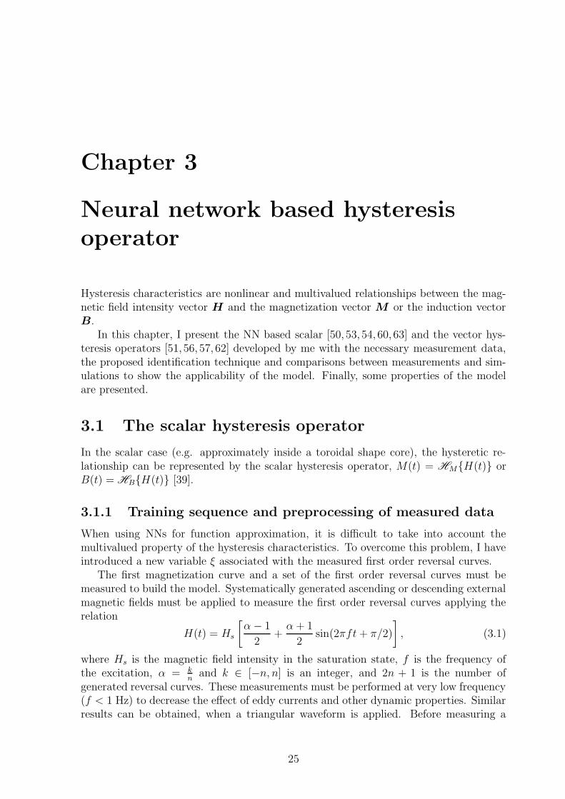
The first magnetization curve and a set of the first order reversal curves must bemeasured to build the model. Systematically generated ascending or descending externalmagnetic fields must be applied to measure the first order reversal curves applying therelation
H(t) = Hs
[α− 1
2+α + 1
2sin(2πft+ π/2)
], (3.1)
where Hs is the magnetic field intensity in the saturation state, f is the frequency ofthe excitation, α = k
nand k ∈ [−n, n] is an integer, and 2n + 1 is the number of
generated reversal curves. These measurements must be performed at very low frequency(f < 1 Hz) to decrease the effect of eddy currents and other dynamic properties. Similarresults can be obtained, when a triangular waveform is applied. Before measuring a
25
Miklos Kuczmann, PhD Theses 2004
−1.5 −0.75 0 0.75 1.5
x 104
−2
−1
0
1
2
H[A/m]
B[T
]
(a) The measured first order reversalcurves
−1
−0.5
0
0.5
1
−1
−0.75
−0.5
−0.25
0−1
−0.5
0
0.5
1
H/Hs
ξ
B/B
s
(b) The normalized and preprocessed firstorder reversal curves
Fig. 3.1. The measured and the preprocessed training sequence
reversal curve, it is advisable to generate some major loops to make a loop stable afteraccommodation.
After measurements, it is useful to work with relative quantities, H/Hs and M/Ms
or B/Bs, so that the input and the output of the model can run in the interval [−1, 1]and the subscript s denotes the saturation state.
If a new variable ξ is added to the measured and normalized first order reversalcurves, the multivalued characteristic can be represented by a single valued 2D surfacewith two independent variables H and ξ. It is enough to measure either the ascendingor the descending branches because of the symmetry of the magnetic hysteresis char-acteristics. The upgrade part of the hysteresis characteristics can be described by apositive real parameter ξ(asc) = 1 − (1 + H
(asc)tp )/2, and the downgrade part can be ap-
proximated by a negative real parameter ξ(desc) = −(1 + H(desc)tp )/2. These parameters
can be calculated for a given transition curve starting from a turning point Htp, andξ(asc) ∈ [0, 1], ξ(desc) ∈ [−1, 0]. The values ±1 represent the major curve, e.g. −1 denotesthe descending curve of the measured major loop.
After preprocessing, the aim is to find the approximating nonlinear functions whichcan be realized by feedforward type NNs trained by the Levenberg-Marquardt BP method[19,25,27]. Two NNs must be used, one to approximate the first magnetization curve andanother one for the preprocessed first order reversal branches. The first magnetizationcurve (about 40 data pairs) can be approximated by a NN with 8 neurons in 1 hiddenlayer (1 input, H and 1 output, M or B), and the preprocessed first order transitioncurves (about 500-800 data pairs give accurate result depending on the shape of thecharacteristic) can be approached by a NN with 2 inputs (H and ξ) and 1 output (Mor B) built by 7, 11 and 6 PEs in three hidden layers. The structure of the NN andthe number of hidden layers and neurons have been set after some trials. The transferfunction of the neurons is selected to be a bipolar sigmoid function.
26
Miklos Kuczmann, PhD Theses 2004PSfrag replacements
...
...
Cor
rect
ion,se
lect
ion
Knowledge–base about
hysteresis characteristics
If–then type rules for
neural network selection
MEMORY
TDL
Hk
Hk−1
Hk
Hk Mk, Bk
η
M = HMH, B = HBH
ξ
Fig. 3.2. The block representation of the scalar model
The training of the two NNs took about 20 minutes on a Celeron 566 MHz com-puter (192 Mbyte RAM) using the Neural Network Toolbox of MATLAB [99]. Whenapplying a training sequence described above to identify the first magnetization curveand the preprocessed first order reversal curves, the stopping criterion MSE = 10−6
can be reached by not more than 500 and 1200 training epochs in the two NNs. Themeasured first order descending curves (containing 46 branches) generated by the exci-tation waveform (3.1) are plotted in Fig. 3.1(a). In this case n = 20, but there are somemeasured curves near the coercive field where the characteristic is very steep and thereis no information enough about the variation of the curves in this area. After applyingthe proposed preprocessing technique, a 2D surface can be obtained as shown in Fig.3.1(b). The training sequence contained 1296 measured points. The measurement wasperformed at f = 0.2 Hz frequency on a toroidal shape C19 structural steel [52]. Inthis case, only technical saturation can be described by the values Hs = 1.433 · 104 A/mand Bs = 1.688 T. Higher magnetic field intensity could not be generated by the ap-plied power supply. The particular presentation of the measurement setup and scalarhysteresis measurements can be found in the section 3.1.4.
3.1.2 Operation of the model
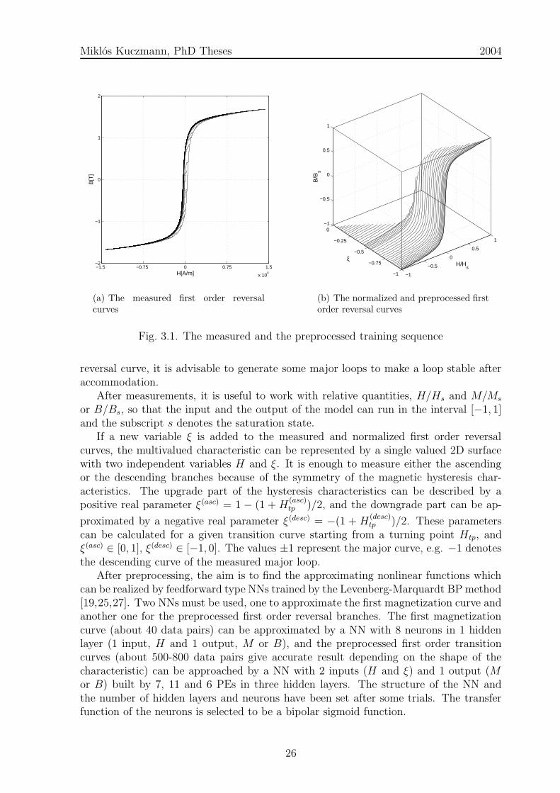
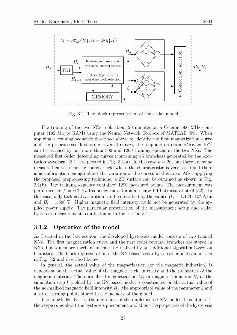
As I stated in the last section, the developed hysteresis model consists of two trainedNNs. The first magnetization curve and the first order reversal branches are stored inNNs, but a memory mechanism must be realized by an additional algorithm based onheuristics. The block representation of the NN based scalar hysteresis model can be seenin Fig. 3.2 and described below.
In general, the actual value of the magnetization (or the magnetic induction) isdependent on the actual value of the magnetic field intensity and the prehistory of themagnetic material. The normalized magnetization Mk or magnetic induction Bk at thesimulation step k yielded by the NN based model is constructed on the actual value ofthe normalized magnetic field intensity Hk, the appropriate value of the parameter ξ anda set of turning points stored in the memory of the model.
The knowledge–base is the main part of the implemented NN model. It contains if–then type rules about the hysteresis phenomena and about the properties of the hysteresis
27
Miklos Kuczmann, PhD Theses 2004
characteristics, and controls the other blocks of the model. The operation of this model isbased on a set of turning points in the ascending and in the descending branches denotedby H
(asc)tp and H
(desc)tp , respectively. Turning points are stored in the memory, that is an
array with the elements [Htp,Mtp, ξ]T or [Htp, Btp, ξ]
T , denoted by MATRIX(asc) andMATRIX(desc) for ascending and descending curves. Turning points can be detected bythe evaluation of a sequence of Hk−1, Hk generated by a tapped delay line (TDL). Afterdetecting a turning point Htp = HSTART = Hk−1 and storing it in the memory, the aim isto select an appropriate transition curve with the right value ξ for the detected turningpoint (Htp,Mtp) or (Htp, Btp), where Mtp = MSTART = Mk−1 or Btp = BSTART = Bk−1.This task has been solved by the regula–falsi method.
There are some basic rules I have implemented in the knowledge–base as if–then typerules. First, a simple lemma about the behavior of the minor loops has been determined:they must be closed as illustrated in Fig. 3.3(a). Therefore the accommodation phe-nomena cannot be simulated yet. After detecting a turning point, the algorithm for ageneral minor loop can be summarized as follows. If MATRIX(desc) (MATRIX(asc))has more than one column and the normalized magnetic field intensity Hk is increasing(decreasing) at the kth simulation step, i.e. Hk > Hk−1 (Hk < Hk−1), then the actual
minor loop must be closed at the last stored value of HGOAL = H(desc)tp (HGOAL = H
(asc)tp )
which can be found in the last column of MATRIX(desc) (MATRIX(asc)). The valueof the normalized magnetization Mk yielded by the NN model at HGOAL must be equalto MGOAL = M
(desc)tp (MGOAL = M
(asc)tp ) stored in the last column of the appropriate
MATRIX (it is also true for magnetic induction). This is the condition for closing aminor loop. The data sets of reached turning points where the actual minor loop isclosing must be cleared from the memory by deleting the appropriate column of thearrays according to the closing minor loop. These are always stored in the last columnof the memory. The first column of the arrays in the memory containing the parametersof the normalized major loop ([+1,+1,−1]T and [−1,−1,+1]T ) cannot be cleared. Thememory mechanism is very similar to the staircase line of the classical Preisach model,but the memory as well as the output of the NN model is continuous in nature and notdiscrete.
The results of simulation have highlighted that, the value of the normalized magneti-zation (induction) yielded by the relevant NN and the adequate value of the normalizedmagnetization (induction) chosen from the appropriate column of the memory at thevalue HGOAL are not equal. Therefore a correction η = η(H,M) (η = η(H,B)) must beused to eliminate this deviation while closing a minor loop. The value of the parameterη can be calculated as the difference between the required value of magnetization (in-duction) and the response of the actual NN at the value of the magnetic field intensityHGOAL when an actual minor loop is closed:
η = MGOAL −M(NN) (HGOAL, ξSTART ) , (3.2)
where ξSTART is the value of the parameter ξ at the actual value of HSTART . Theparameter η must be calculated beforehand when opening a minor loop and must beapplied increasing linearly during the magnetization process from zero (when the minorloop is opening) to the given value η (when the minor loop is closing).
An additional precept must be used as formulated in the following rule: symmet-ric hysteresis loops are assumed (see Fig. 3.3(b)). After the detection of a turning
28
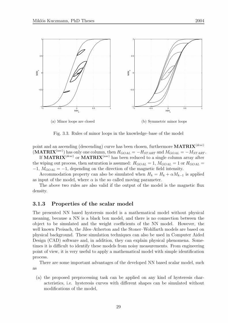
Miklos Kuczmann, PhD Theses 2004
−1 −0.5 0 0.5 1−1
−0.5
0
0.5
1
H/Hs
M/M
s
(a) Minor loops are closed
−1 −0.5 0 0.5 1−1
−0.5
0
0.5
1
H/Hs
M/M
s
(b) Symmetric minor loops
Fig. 3.3. Rules of minor loops in the knowledge–base of the model
point and an ascending (descending) curve has been chosen, furthermore MATRIX(desc)
(MATRIX(asc)) has only one column, thenHGOAL = −HSTART andMGOAL = −MSTART .If MATRIX(desc) or MATRIX(asc) has been reduced to a single column array after
the wiping out process, then saturation is assumed: HGOAL = 1, MGOAL = 1 or HGOAL =−1, MGOAL = −1, depending on the direction of the magnetic field intensity.
Accommodation property can also be simulated when Hk = Hk + αMk−1 is appliedas input of the model, where α is the so called moving parameter.
The above two rules are also valid if the output of the model is the magnetic fluxdensity.
3.1.3 Properties of the scalar model
The presented NN based hysteresis model is a mathematical model without physicalmeaning, because a NN is a black box model, and there is no connection between theobject to be simulated and the weight coefficients of the NN model. However, thewell known Preisach, the Jiles–Atherton and the Stoner–Wohlfarth models are based onphysical background. These simulation techniques can also be used in Computer AidedDesign (CAD) software and, in addition, they can explain physical phenomena. Some-times it is difficult to identify these models from noisy measurements. From engineeringpoint of view, it is very useful to apply a mathematical model with simple identificationprocess.
There are some important advantages of the developed NN based scalar model, suchas
(a) the proposed preprocessing task can be applied on any kind of hysteresis char-acteristics, i.e. hysteresis curves with different shapes can be simulated withoutmodifications of the model,
29

Miklos Kuczmann, PhD Theses 2004
−800 −400 0 400 800−1.6
−0.8
0
0.8
1.6
H [A/m]
B [T
]
SimulatedMeasured
(a) Hmax = 718 A/m
−4000 −2000 0 2000 4000−1.6
−0.8
0
0.8
1.6
H [A/m]
B [T
]
SimulatedMeasured
(b) Hmax = 3580 A/m
−6000 −3000 0 3000 6000−1.6
−0.8
0
0.8
1.6
H [A/m]
B [T
]
SimulatedMeasured
(c) Hmax = 5750 A/m
Fig. 3.4. Comparisons between the simulated and the measured symmetric minor loops
0 2 4 6 8 10 12 14 16 18 200
5
10
15
20
25
Minor loop
∆Wm
[%]
Fig. 3.5. The error in the hysteresis area between the measured and the simulatedcharacteristics
(b) the identification of the scalar model is an easy task, once the measured firstmagnetization curve and the first order reversal branches are known,
(c) the output of the model, i.e. the normalized magnetization or the normalizedinduction is a continuous function of the magnetic field intensity, because NNs caninterpolate between trained data according to the generalization property of theNNs,
(d) if necessary, the differential susceptibility χdiff as well as the integral of the outputof the model (e.g. to calculate hysteresis losses) can be expressed in analyticalform.
It is very important to verify a NN based model by comparing the simulated andthe measured data which were not contained in the training sequence. I have measuredsymmetric minor loops, and the comparison between measurements and simulations canbe seen in Fig. 3.4(a), Fig. 3.4(b) and Fig. 3.4(c). The maximum value of the calculatederror 4B = 100|(Bm − Bs)/Bm,s| is 35%, 10% and 8% respectively, where Bm and Bs
30

Miklos Kuczmann, PhD Theses 2004
are the measured and the simulated induction, respectively, and Bm,s = 1.688 T is themeasured induction in the saturation state. The maximum difference can be locatednear the coercive field as highlighted in the figures. The measured major loop and themeasured first order reversal curves (i.e. the training sequence) can be approximatedwith an error value less than maximum 4− 5%.
To compare the measured and the simulated characteristics, the hysteresis losses fromthe enclosed area of the hysteresis loops are determined for 20 measured and simulatedsymmetric minor loops. The calculated relative error in the losses with respect to themeasured curves is plotted in Fig. 3.5.
3.1.4 Scalar magnetic hysteresis measurement using LabVIEW
Ferromagnetic hysteresis measurement has been performed in our Magnetic Laboratoryby a computer controlled automated measuring system [47, 48, 52]. Generation of exci-tation and measurements are carried out by applying the user–friendly environment ofLabVIEW. The graphical user interface of the developed software is illustrated in Fig.3.6, data and graphs in the window are presented briefly below.
LabVIEW is an application software to perform sophisticated display and analy-sis capabilities required for virtual instrumentation. This can be used to create testmeasurement systems by combining different hardware and software components. Dataacquisition and waveform generation can be carried out by virtual software instrumentsand tools, and the measurement can be realized by plug–in hardware connected to thecomputer via special National Instruments driver software [38].
Schematic view of the measurement set–up can be seen in Fig. 3.7. The investigatedferromagnetic sample has toroidal shape. It is supposed that, both the magnetic fieldintensity with its scalar value H and the magnetic induction B are uniform inside thematerial and directed along the axis of the toroidal core. This results in a scalar hysteresischaracteristic. The excitation coil is excited by the current i(t) supplied by the powergenerator KIKUSUI [22] and the current waveform is measured by the voltage of thetemperature and voltage independent resistor of R = 0.01 Ω (i(t) = uP (t)/R). Themeasured magnetic field intensity is proportional to the exciting current and can becalculated as
H(t) =Np i(t)
l, (3.3)
where Np = 170 is the number of turns of the excitation (primary) coil, i(t) is theexcitation current and l = 176 mm is the equivalent magnetic length of the toroidalcore. The magnetic flux density B can be calculated from the measured induced voltageof the measuring (secondary) coil us(t) as
B(t) = B0 +1
S Ns
∫ t
0
us(τ) dτ, (3.4)
where B0 is an integration constant, S = 20 mm2 is the cross-section of the core andNs = 182 is the number of turns of the measuring coil. The measured signals, thecalculated waveform of the magnetic field intensity and of the magnetic flux density andthe resulted hysteresis characteristic are visualized in the user interface (see Fig. 3.6).
Measurements are performed by using the LabVIEW environment. The computercommunicates with the measuring instruments through an NI–DAQ (National Instru-ments, Data Acquisition Device) BNC–2090 panel which is connected to the DAQ
31
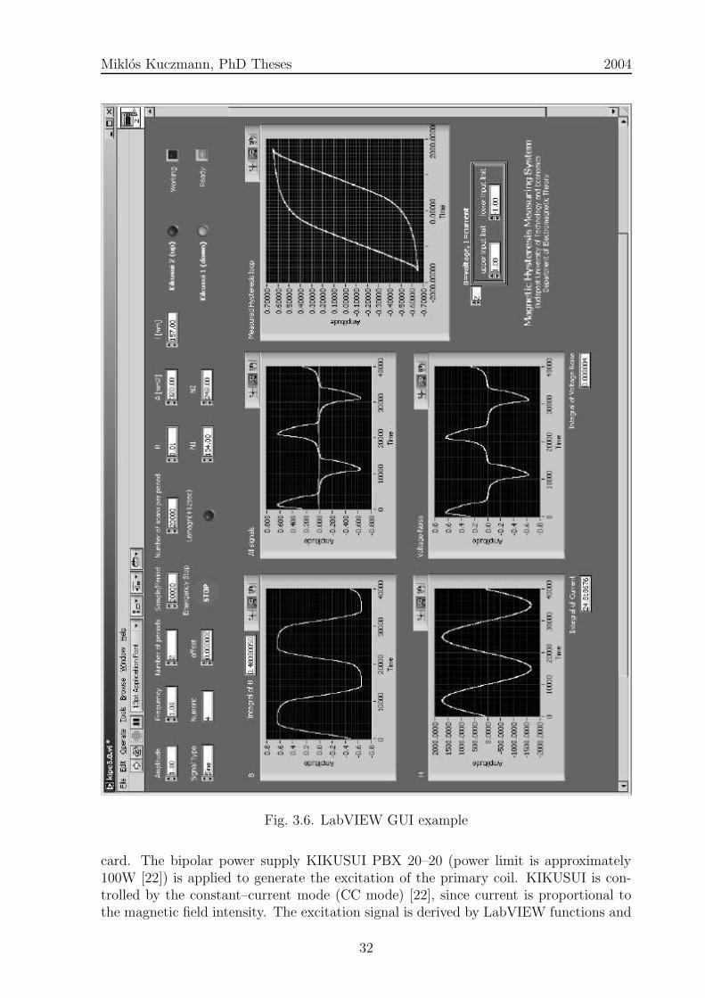
Miklos Kuczmann, PhD Theses 2004
Fig. 3.6. LabVIEW GUI example
card. The bipolar power supply KIKUSUI PBX 20–20 (power limit is approximately100W [22]) is applied to generate the excitation of the primary coil. KIKUSUI is con-trolled by the constant–current mode (CC mode) [22], since current is proportional tothe magnetic field intensity. The excitation signal is derived by LabVIEW functions and
32

Miklos Kuczmann, PhD Theses 2004
PSfrag replacements
SR
up(t) us(t)
i(t)
Np Ns
l
Φ
KIKUSUI PBX 20–20 Computer
Waveform of excitation current
Data
Acq
uisition
Dev
ice
Fig. 3.7. Schematic view of the scalar hysteresis measurement set–up
the power supply can follow this signal by the analog output of the BNC panel. Theinduced voltage is measured by using the same DAQ card. Data acquisition and genera-tion of the excitation current can be performed simultaneously by using the intermediatevirtual instruments (circular buffered waveform generation and measurement) [38].
Measured curves are saved to a file, for further use of the measured data using othersoftware or for a report. The waveform, the amplitude and the frequency of the excitationcurrent, the number of measured periods and of measured samples in one period, andother parameters (Np, Ns, S, l, R) can be set through the graphical user interface.
Computer–aided measurements can only be performed by sampling using A/D andD/A converters (acquisition) [38]. This can be carried out through general DAQ devices,GPIB interfaces, RS–232 instruments and so on. This may be a weak point of themeasurement process if very steep signals must be measured (e.g. induced voltage inthe secondary coil), but it can be eliminated by the appropriate choice of the samplingrate. The main advantage of applying computer controlled measurement is the dataanalysis, such as curve fitting, frequency response, filtering, Fourier analysis and manyother numerical operations realized by a software.
33

Miklos Kuczmann, PhD Theses 2004
3.2 The isotropic vector hysteresis operator
3.2.1 Description of the model
The vector NN based model of the magnetic hysteresis is constructed as a superpositionof scalar NN based models. The magnetization vector M can be expressed in twodimensions as
M =
∫ π/2
−π/2
eϕ H Hϕ dϕ, (3.5)
where Mϕ = H Hϕ is the scalar magnetization in the direction eϕ, and the projectedmagnetic field intensity is Hϕ = |H| cos(ϑH − ϕ) with the direction of the magnetic fieldintensity vector H , denoted by ϑH . First, I have analyzed the isotropic vector hysteresischaracteristic, when the same NN based scalar hysteresis operator H · has been usedin all directions.
In computer realization, it is useful to discretize the interval ϕ ∈ [−π/2, π/2] asϕi = −π/2 + (i − 1)π/n′, where i = 1, . . . , n′, and n′ is the number of directions. Themagnetization vector is the vectorial sum of the scalar magnetization yielded by theindividual scalar hysteresis models, i.e. (see Fig. 3.8)
M ∼=
n′∑
i=1
eϕiMϕi
=
n′∑
i=1
eϕiH Hϕi
. (3.6)
In three dimensions, the following expression can be obtained,
M =
∫ π/2
−π/2
∫ π/2
−π/2
eϕ,ϑ H Hϕ,ϑ dϕ dϑ, (3.7)
where the projected magnetic field intensity is Hϕ,ϑ = [a1 a2 a3]ϕ,ϑ[HxHyHz]T , and the
directions are given as a = a1ex + a2ey + a3ez, |a| = 1 corresponding to the given di-rections allocated by the angles ϕ and ϑ as shown in Fig. 3.9(a) and generated by anicosahedron (see Fig. 3.9(b)). The angles ϕ and ϑ are measured from the x–axis andfrom the x − y plane, respectively. Any kind of regular 3D formation can be used (likepolyhedrons, e.g. cube, octahedron, dodecahedron and so on), but I have found that, theicosahedron gives the best results. The applied scalar hysteresis operator is also uniquefor all directions. The integral formula (3.7) can be realized by a numerical sum in thediscrete form
M ∼=
n′∑
i=1
eϕi,ϑiMϕi,ϑi
=n′∑
i=1
eϕi,ϑiH Hϕi,ϑi
, (3.8)
where n′ is the number of directions in the 3D space.
3.2.2 The identification process
I have measured the Everett function in the x direction, then the following well knowntrivial condition can be obtained between the measured scalar Everett function F (α, β)and the unknown 2D vector Everett function E(α, β) [67]:
F (α, β) =
∫ π/2
−π/2
cosϕE(α cosϕ, β cosϕ) dϕ. (3.9)
34
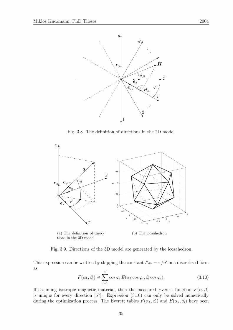
Miklos Kuczmann, PhD Theses 2004
PSfrag replacements
x
y
ex
ey
1
2
n′
. ..
...
i
H
Hϕi
eϕiϕi
ϑH
Fig. 3.8. The definition of directions in the 2D model
PSfrag replacements
x
z
y
ex
ey
ez
ϕ
ϑ
a
eϕ,ϑ
(a) The definition of direc-tions in the 3D model
−1−0.5
00.5
1
−1
−0.5
0
0.5
1−1
−0.5
0
0.5
1
x
y
z
(b) The icosahedron
Fig. 3.9. Directions of the 3D model are generated by the icosahedron
This expression can be written by skipping the constant 4ϕ = π/n′ in a discretized formas
F (αk, βl) ∼=
n′∑
i=1
cosϕiE(αk cosϕi, βl cosϕi). (3.10)
If assuming isotropic magnetic material, then the measured Everett function F (α, β)is unique for every direction [67]. Expression (3.10) can only be solved numericallyduring the optimization process. The Everett tables F (αk, βl) and E(αk, βl) have been
35

Miklos Kuczmann, PhD Theses 2004
PSfrag replacements
α
1
αjαj−1 αkαk−1
E(αk, 0)E(αk−1, 0)E(αj, 0)E(αj−1, 0)
. . . . . . . . .n′1αk cosϕi1 αk cosϕi2
1 . . . n′2
Fig. 3.10. Illustration for the first step of the identification, when α ≥ 0 and β = 0
divided into (N + 1)× (N + 1) parts, with k, l = 1, . . . , N + 1, αk = 2N
(k − N+1
2
)− 1
N,
βl = 2N
(N+1
2− l)
+ 1N
. In this case α ∈ [−1, . . . ,+1], β ∈ [+1, . . . ,−1] and N must bean even number.
In the 3D case, the expression (3.10) can also be applied, but ϕi is then the spatialangle between the directions generated by the icosahedron and the x–axis.
The identification process is divided into two main parts. In the first step, the partof the Everett function can be identified where β = 0 and α = −β. In the second step,the other parts can be calculated step by step by using values from the first step andsome points from the second step.
The first step: starting the identification process
I have developed the identification technique on the basis of the above process as de-scribed in the following.
A part of the Everett function is independent of one of the two variables α and βalong the line α ≥ 0 and β = 0, i.e. k = N
2+ 1, . . . , N + 1 and l = N
2+ 1,
F (αk, 0) ∼=
n′∑
i=1
cosϕiE(αk cosϕi, 0). (3.11)
In this case, the Everett function can be divided into two parts. The first n′1 points are
known, but the other n′2 points contain the unknown part of the vector Everett function
E(αk, 0),
F (αk, 0) ∼=
n′
1∑
i1=1
cosϕi1 E(αk cosϕi1, 0)
+
n′
2∑
i2=1
cosϕi2 E(αk cosϕi2, 0).
(3.12)
When αj−1 < αk cosϕi1 ≤ αj and αj−1 < αj ≤ αk−1 and assuming linear interpolationbetween known points of the vector Everett function (αj−1, E(αj−1, 0)) and (αj, E(αj, 0)),the following formula –illustrated in Fig. 3.10– can be applied to interpolate a givenvalue,
E(αj, 0)− E(αj−1, 0)
αj − αj−1
=E(αk cosϕi1 , 0)− E(αj−1, 0)
αk cosϕi1 − αj−1
, (3.13)
from which
E(αk cosϕi1 , 0) = E(αj−1, 0) +αk cosϕi1 − αj−1
αj − αj−1
×(E(αj, 0)− E(αj−1, 0)
).
(3.14)
36

Miklos Kuczmann, PhD Theses 2004
This expression contains known values of the vector Everett function calculated inthe previous steps. The number of known points increases with the index k. Whenαk−1 < αk cosϕi2 ≤ αk, then a similar expression can be used:
E(αk, 0)− E(αk−1, 0)
αk − αk−1
=E(αk cosϕi2 , 0)− E(αk−1, 0)
αk cosϕi2 − αk−1
, (3.15)
from which
E(αk cosϕi2 , 0) = E(αk−1, 0) +αk cosϕi2 − αk−1
αk − αk−1
×(E(αk, 0)− E(αk−1, 0)
).
(3.16)
This contains the only one unknown point of the vector Everett function E(αk, 0). Thefollowing expression can be obtained by substituting the relations (3.14) and (3.16) intothe equation (3.12):
F (αk, 0) =
n′
1∑
i1=1
cosϕi1
E(αj−1, 0)
+αk cosϕi1 − αj−1
αj − αj−1
(E(αj, 0)− E(αj−1, 0)
)
+E(αk−1, 0)((1 + bk)c1 − akc2
)
+E(αk, 0)(akc2 − bkc1
),
(3.17)
where ak = αk
αk−αk−1, bk =
αk−1
αk−αk−1, c1 =
∑n′
2i2=1 cosϕi2 , and c2 =
∑n′
2i2=1 cos2 ϕi2 and
E(αk, 0) can be expressed.A similar mathematical formulation can be obtained along the line α = −β. In this
case, the indices k and l are in the interval [N2
+ 1, . . . , N + 1]. According to the linearinterpolation between two points, the following expressions can be obtained after somemathematical manipulations. If αj−1 = βj−1 < αk cosϕi1 = βl cosϕi1 ≤ αj = βj andαj−1 = βj−1 < αj = βj ≤ αk−1 = βk−1, then the known point in the Everett functioncan be expressed as
E(αk cosϕi1 , βl cosϕi1) = E(αj−1, βj−1)
+
√α2k cos2 ϕi1 + β2
l cos2 ϕi1 −√α2j−1 + β2
j−1√α2j + β2
j −√α2j−1 + β2
j−1
×(E(αj, βj)− E(αj−1, βj−1)
).
(3.18)
If αk−1 = βk−1 < αk cosϕi2 = βl cosϕi2 ≤ αk = βk, then the unknown point in theEverett function can be expressed as
E(αk cosϕi2, βl cosϕi2) = E(αk−1, βl−1)
+
√α2k cos2 ϕi2 + β2
l cos2 ϕi2 −√α2k−1 + β2
l−1
√α2k + β2
l −√α2k−1 + β2
l−1
×(E(αk, βl)− E(αk−1, βl−1)
).
(3.19)
Here E(αk, βl) is the only unknown, and it can be expressed after substituting the re-lations (3.18) and (3.19) into (3.10). This generates some points in the vector Everettfunction and gives an initiative step to determine the other values.
37

Miklos Kuczmann, PhD Theses 2004
PSfrag replacements
0
0
0
0
0
0
0
0
0
. . .
...
. .. . . . . . .
...
. ..
. ..
. . .
. . .
. . .
α
β
(αk, βl)
(αk, βl−1)
(αk−1, βl)(α1, β1)
(α2, β2)(α3, β3)Known Unknown
Fig. 3.11. Illustration for the second step of the identification process
The second step: the other points on the vector Everett plane
I have divided the vector Everett function into triangles and I have applied linear inter-polation on these triangles to calculate the values on the Everett functions correspondingto the coordinates (αk cosϕ, βl cosϕ). An explanatory plot with notations can be seenin Fig. 3.11.
In this case, the Everett function can also be divided into two parts. The first n′1
points are known, but the other n′2 points contain the unknown part of the vector Everett
function E(αk, βl),
F (αk, βl) ∼=
n′
1∑
i1=1
cosϕi1 E(αk cosϕi1 , βl cosϕi1)
+
n′
2∑
i2=1
cosϕi2 E(αk cosϕi2 , βl cosϕi2).
(3.20)
If α > 0 and β < 0 (k = l + 1, . . . , N + 1, l = N2
+ 2, . . . , N + 1) and the point(αk cosϕi1 , βl cosϕi1) is on a triangle with known node values, then the equation of aplane with three points e.g. (αk−1, βl, E1), (αk, βl−1, E2) and (αk−1, βl−1, E3) can beapplied as ∣∣∣∣∣∣
αk cosϕi1 − α1 βl cosϕi1 − β1 E − E1
α2 − α1 β2 − β1 E2 − E1
α3 − α1 β3 − β1 E3 − E1
∣∣∣∣∣∣= 0, (3.21)
where α1 = αk−1, β1 = βl, α2 = αk, β2 = βl−1, α3 = αk−1, β3 = βl−1, E1 = E(αk−1, βl),E2 = E(αk, βl−1), E3 = E(αk−1, βl−1) and E = E(αk cosϕi1 , βl cosϕi1). From this
38

Miklos Kuczmann, PhD Theses 2004
equation
E(αk cosϕi1, βl cosϕi1) = E1−(αk cosϕi1 − α1)(cf − ed)
(ad− bc)
−(βl cosϕi1 − β1)(be− af)
(ad− bc),
(3.22)
where a = α2−α1, b = α3−α1, c = β2− β1, d = β3− β1, e = E2−E1 and f = E3−E1.Varying these three points, the equation of any other triangles with known node valuescan be represented and known points can be calculated.
If point (αk cosϕi2 , βl cosϕi2) is on a triangle which contains the unknown value ofthe vector Everett function E(αk, βl), then the equation of a plane with the three points(αk−1, βl, E1), (αk, βl, E2) and (αk, βl−1, E3) can be applied as
∣∣∣∣∣∣
αk cosϕi2 − αk−1 βl cosϕi2 − βl E − E1
αk − αk−1 βl − βl E2 − E1
αk − αk−1 βl−1 − βl E3 − E1
∣∣∣∣∣∣= 0, (3.23)
where E1 = E(αk−1, βl), E2 = E(αk, βl), E3 = E(αk, βl−1) and E = E(αk cosϕi2 , βl cosϕi2).From this equation
E(αk cosϕi2 , βl cosϕi2) = E1
+(βl−1 − βl)(αk cosϕi2 − αk−1)(E2 − E1)
(αk − αk−1)(βl−1 − βl)
−(αk − αk−1)(βl cosϕi2 − βl)(E2 − E3)
(αk − αk−1)(βl−1 − βl)
(3.24)
can be obtained which contains the unknown value E2. Substituting (3.22) and (3.24)into (3.20) E2 can be expressed for all indices k and l.
If α > 0 and β > 0 (k = N +3− l, . . . , N +1, l = N2, . . . , 1), then a similar procedure
can be applied, but the shape of the triangles is different.The Everett function is symmetrical with respect to the line α = −β, so it is enough
to identify only the half of the vector Everett function.
3.2.3 Verification of the model
To illustrate the above process, I have assumed that, the measured Everett function isgiven in the x direction and it is plotted in Fig. 3.12(a). The identified 2D vector Everettfunction, and the identified 3D vector Everett function are shown in Fig. 3.12(b) andFig. 3.12(c).
Identification has been performed by the method described above, 20 directions and9 directions have been used in the 2D and in the 3D model, respectively. The measuredscalar Everett surface can be approximated with a relative error below 0.3% and 0.4%by the 2D and the 3D models by substituting into the trivial condition (3.10). Theresulting vector Everett functions –as highlighted in the figures– do not have the usualshape, meaning that, the first order reversal curves also do not have the usual descendingshape, but they can be approximated easily by the scalar NN based hysteresis model.
First order reversal curves can be derived from the identified vector Everett function,and NNs can be trained as well as models can be built by trained NNs. A comparison
39

Miklos Kuczmann, PhD Theses 2004
−1
−0.5
0
0.5
1
−1
−0.5
0
0.5
10
0.25
0.5
0.75
1
αβ
F(α
,β)
(a) The measured Everettfunction in the x direction
−1
−0.5
0
0.5
1
−1
−0.5
0
0.5
10
0.025
0.05
0.075
0.1
αβ
E(α
,β)
(b) The identified 2D vec-tor Everett function
−1
−0.5
0
0.5
1
−1
−0.5
0
0.5
1−0.05
0
0.05
0.1
0.15
αβ
E(α
,β)
(c) The identified 3D vec-tor Everett function
Fig. 3.12. Identification results of the isotropic vector hysteresis model
−1 −0.5 0 0.5 1−1
−0.5
0
0.5
1
Hx/H
s
Mx/M
s
(a) Comparison in 2D
−1 −0.5 0 0.5 1−1
−0.5
0
0.5
1
Hx/H
s
Mx/M
s
(b) Comparison in 3D
Fig. 3.13. Identification results for isotropic case
between measured (denoted by points) and simulated first order reversal curves by theidentified 2D and 3D models (denoted by dotted line) can be seen in Fig. 3.13(a) andFig. 3.13(b).
Some other verification and comparisons with the anisotropic model are presented atthe end of this chapter.
40

Miklos Kuczmann, PhD Theses 2004
3.3 The anisotropic vector hysteresis operator
The anisotropic vector NN based model of magnetic hysteresis is also constructed as asuperposition of scalar NN based models in the directions eϕ, but these scalar hysteresischaracteristics are not the same. The magnetization vector M can be expressed in twodimensions as (see Fig. 3.8)
M =
∫ π/2
−π/2
eϕ HϕHϕ dϕ. (3.25)
In three dimensions a similar expression can be obtained (see Fig. 3.9(a)):
M =
∫ π/2
−π/2
∫ π/2
−π/2
eϕ,ϑ Hϕ,ϑHϕ,ϑ dϕ dϑ. (3.26)
The main point of my research was to handle the angular dependence of the hysteresischaracteristics, and applying the same identification process with minor modificationsas used in the isotropic case. The Fourier expansion on the Everett surfaces can be usedefficiently, when assuming uniaxial anisotropy.
3.3.1 Anisotropic model in 2D
I have assumed that, the scalar Everett function can be measured in any given direc-tion. This is the scalar characterization of the vector hysteresis property. In this case,the following condition can be obtained between the measured scalar Everett functionF (α, β, ϕ) and the unknown vector Everett function E(α, β, ϕ):
F (α, β, ϕ) =
∫ π/2
−π/2
cosψ E(α cosψ, β cosψ, ψ + ϕ) dψ, (3.27)
and this expression can be derived in a discretized form as
F (αk, βl, ϕj) ∼=
n′∑
i=1
cosψiE(αk cosψi, βl cosψi, ϕi), (3.28)
where ψi = ϕi − ϕj is the angle between the direction of the measured scalar Everettfunction in the direction eϕj
and the unknown vector Everett function in the directioneϕi
. The identification process is based on n′ directions, ϕi ∈ [−π/2, . . . , π/2], selectedas ϕi = −π/2+(i−1)π/n′, where i = 1, . . . , n′. Assuming that the material has uniaxialanisotropy, the measured scalar Everett function must be π-periodic and an even functionwith respect to ϕ, if ϕ = 0 represents the rolling direction and ϕ = π/2 is perpendicularto the rolling direction (transverse direction), i.e.
F (αk, βl, ϕj + π) = F (αk, βl, ϕj), (3.29)
andF (αk, βl,−ϕj) = F (αk, βl, ϕj). (3.30)
I supposed that, there are n + 1 measured Everett functions F (αk, βl, ϕj) in theinterval ϕj ∈ [0, . . . , π/2], ϕj = j∆ϕ, ∆ϕ = π/2n and j = 0, . . . , n, and n′ is chosen asn′ = 2n as plotted in Fig. 3.14.
41

Miklos Kuczmann, PhD Theses 2004
PSfrag replacements
x
y
n
0
j
ϕj
. . .
Fig. 3.14. The directions of the measured Everett functions F (α, β, ϕ)
−1
−0.5
0
0.5
1
−1
−0.5
0
0.5
10
0.25
0.5
0.75
1
αβ
Fx(α
,β)
(a) The Everett function in therolling direction, ϕ = 0
−1
−0.5
0
0.5
1
−1
−0.5
0
0.5
10
0.25
0.5
0.75
1
αβ
Fy(α
,β)
(b) The Everett function in thetransverse direction, ϕ = π/2
Fig. 3.15. The measured Everett functions to build the 2D anisotropic vector hysteresismodel in (3.31)
In my experiments, I assumed to have n + 1 = 10 scalar hysteresis characteristics,i.e. ϕ0 = 0, ϕ1 = 10, . . . , ϕ9 = 90, generated by the elliptical interpolation function
F (ϕ) = F 2x cos2 ϕ+ F 2
y sin2 ϕ, (3.31)
where F (ϕ) = F (α, β, ϕ), Fx = F (α, β, 0) and Fy = F (α, β, π/2) are the assumednormalized Everett functions in the rolling and in the transverse directions, respectively,and plotted in Fig. 3.15(a) and Fig. 3.15(b).
Due to the periodicity of the measured Everett function, it can be approximatedby its Fourier series. It is difficult to take into account the angular dependence of themeasured Everett function during the identification process, but the Fourier expansion isan accurate method to handle this phenomenon. Since F (α, β, ϕ) is an even function withrespect to ϕ, only the real part of the complex Fourier series must be calculated (to makethe equations below shorter, the following notation will be used: F (ϕj) = F (αk, βl, ϕj)),
42
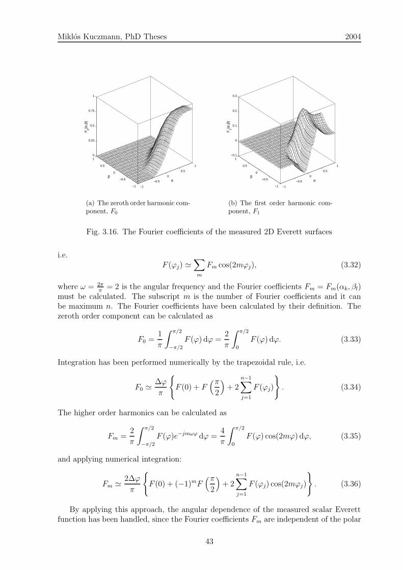
Miklos Kuczmann, PhD Theses 2004
−1
−0.5
0
0.5
1
−1
−0.5
0
0.5
10
0.25
0.5
0.75
1
αβ
F0(α
,β)
(a) The zeroth order harmonic com-ponent, F0
−1
−0.5
0
0.5
1
−1
−0.5
0
0.5
1−0.1
0
0.1
0.2
0.3
αβ
F1(α
,β)
(b) The first order harmonic com-ponent, F1
Fig. 3.16. The Fourier coefficients of the measured 2D Everett surfaces
i.e.F (ϕj) '
∑
m
Fm cos(2mϕj), (3.32)
where ω = 2ππ
= 2 is the angular frequency and the Fourier coefficients Fm = Fm(αk, βl)must be calculated. The subscript m is the number of Fourier coefficients and it canbe maximum n. The Fourier coefficients have been calculated by their definition. Thezeroth order component can be calculated as
F0 =1
π
∫ π/2
−π/2
F (ϕ) dϕ =2
π
∫ π/2
0
F (ϕ) dϕ. (3.33)
Integration has been performed numerically by the trapezoidal rule, i.e.
F0 '∆ϕ
π
F (0) + F
(π2
)+ 2
n−1∑
j=1
F (ϕj)
. (3.34)
The higher order harmonics can be calculated as
Fm =2
π
∫ π/2
−π/2
F (ϕ)e−jmωϕ dϕ =4
π
∫ π/2
0
F (ϕ) cos(2mϕ) dϕ, (3.35)
and applying numerical integration:
Fm '2∆ϕ
π
F (0) + (−1)mF
(π2
)+ 2
n−1∑
j=1
F (ϕj) cos(2mϕj)
. (3.36)
By applying this approach, the angular dependence of the measured scalar Everettfunction has been handled, since the Fourier coefficients Fm are independent of the polar
43
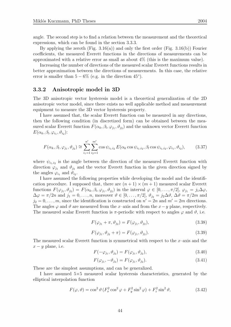
Miklos Kuczmann, PhD Theses 2004
angle. The second step is to find a relation between the measurement and the theoreticalexpressions, which can be found in the section 3.3.3.
By applying the zeroth (Fig. 3.16(a)) and only the first order (Fig. 3.16(b)) Fouriercoefficients, the measured Everett functions in the directions of measurements can beapproximated with a relative error as small as about 4% (this is the maximum value).
Increasing the number of directions of the measured scalar Everett functions results inbetter approximation between the directions of measurements. In this case, the relativeerror is smaller than 5− 6% (e.g. in the direction 45).
3.3.2 Anisotropic model in 3D
The 3D anisotropic vector hysteresis model is a theoretical generalization of the 2Danisotropic vector model, since there exists no well applicable method and measurementequipment to measure the 3D vector hysteresis property.
I have assumed that, the scalar Everett function can be measured in any directions,then the following condition (in discretized form) can be obtained between the mea-sured scalar Everett function F (αk, βl, ϕj1, ϑj2) and the unknown vector Everett functionE(αk, βl, ϕi1 , ϑi2):
F (αk, βl, ϕj1, ϑj2)∼=
n′∑
i1=1
m′∑
i2=1
cosψi1,i2 E(αk cosψi1,i2, βl cosψi1,i2, ϕi1, ϑi2), (3.37)
where ψi1,i2 is the angle between the direction of the measured Everett function withdirection ϕj1 and ϑj2 and the vector Everett function in the given direction signed bythe angles ϕi1 and ϑi2 .
I have assumed the following properties while developing the model and the identifi-cation procedure. I supposed that, there are (n+ 1)× (m+ 1) measured scalar Everettfunctions F (ϕj1, ϑj2) = F (αk, βl, ϕj1, ϑj2) in the interval ϕ ∈ [0, . . . , π/2], ϕj1 = j1∆ϕ,∆ϕ = π/2n and j1 = 0, . . . , n, moreover ϑ ∈ [0, . . . , π/2], ϑj2 = j2∆ϑ, ∆ϑ = π/2m andj2 = 0, . . . , m, since the identification is constructed on n′ = 2n and m′ = 2m directions.The angles ϕ and ϑ are measured from the x–axis and from the x−y plane, respectively.The measured scalar Everett function is π-periodic with respect to angles ϕ and ϑ, i.e.
F (ϕj1 + π, ϑj2) = F (ϕj1, ϑj2), (3.38)
F (ϕj1, ϑj2 + π) = F (ϕj1, ϑj2). (3.39)
The measured scalar Everett function is symmetrical with respect to the x–axis and thex− y plane, i.e.
F (−ϕj1, ϑj2) = F (ϕj1, ϑj2), (3.40)
F (ϕj1,−ϑj2) = F (ϕj1, ϑj2). (3.41)
These are the simplest assumptions, and can be generalized.I have assumed 5×5 measured scalar hysteresis characteristics, generated by the
elliptical interpolation function
F (ϕ, ϑ) = cos2 ϑ (F 2x cos2 ϕ+ F 2
y sin2 ϕ) + F 2z sin2 ϑ, (3.42)
44
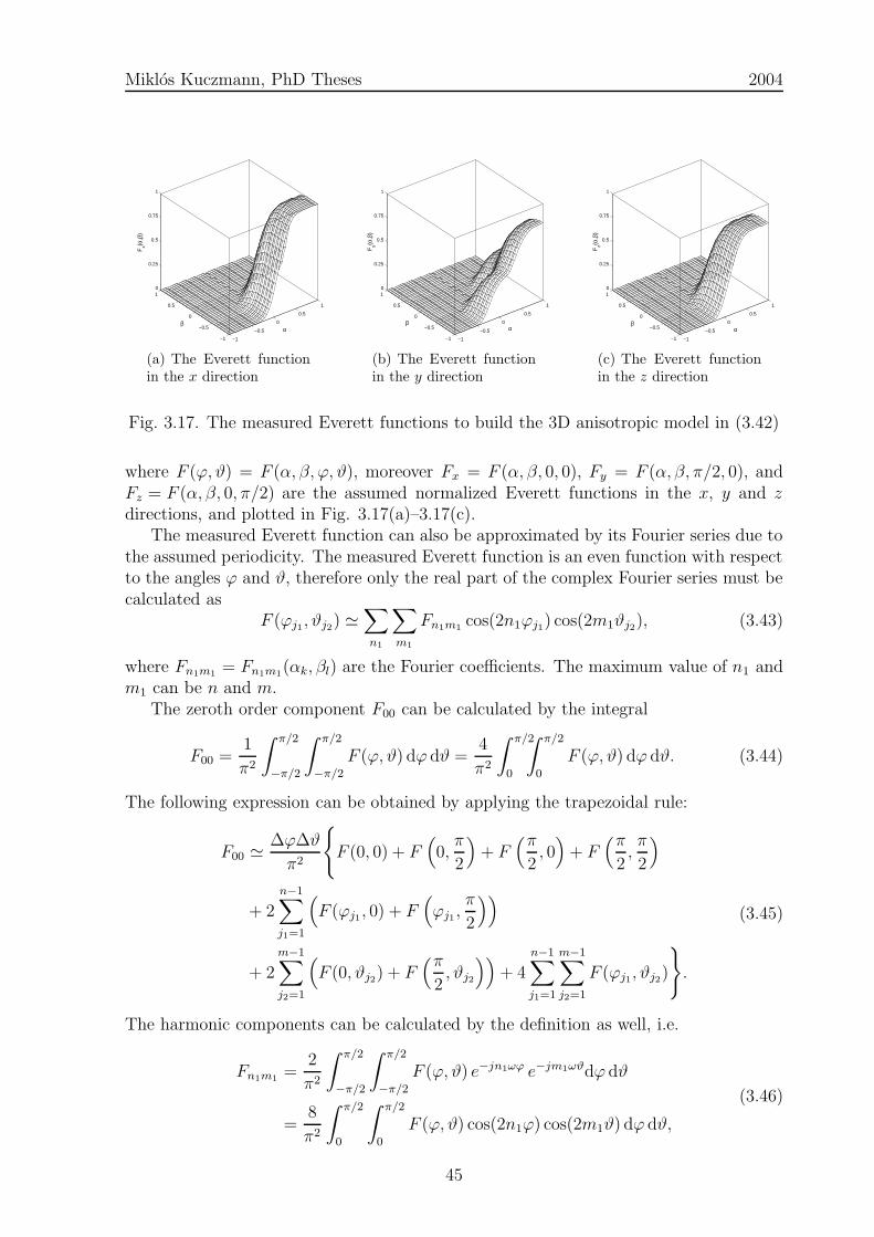
Miklos Kuczmann, PhD Theses 2004
−1
−0.5
0
0.5
1
−1
−0.5
0
0.5
10
0.25
0.5
0.75
1
αβ
Fx(α
,β)
(a) The Everett functionin the x direction
−1
−0.5
0
0.5
1
−1
−0.5
0
0.5
10
0.25
0.5
0.75
1
αβ
Fy(α
,β)
(b) The Everett functionin the y direction
−1
−0.5
0
0.5
1
−1
−0.5
0
0.5
10
0.25
0.5
0.75
1
αβ
Fz(α
,β)
(c) The Everett functionin the z direction
Fig. 3.17. The measured Everett functions to build the 3D anisotropic model in (3.42)
where F (ϕ, ϑ) = F (α, β, ϕ, ϑ), moreover Fx = F (α, β, 0, 0), Fy = F (α, β, π/2, 0), andFz = F (α, β, 0, π/2) are the assumed normalized Everett functions in the x, y and zdirections, and plotted in Fig. 3.17(a)–3.17(c).
The measured Everett function can also be approximated by its Fourier series due tothe assumed periodicity. The measured Everett function is an even function with respectto the angles ϕ and ϑ, therefore only the real part of the complex Fourier series must becalculated as
F (ϕj1, ϑj2) '∑
n1
∑
m1
Fn1m1 cos(2n1ϕj1) cos(2m1ϑj2), (3.43)
where Fn1m1 = Fn1m1(αk, βl) are the Fourier coefficients. The maximum value of n1 andm1 can be n and m.
The zeroth order component F00 can be calculated by the integral
F00 =1
π2
∫ π/2
−π/2
∫ π/2
−π/2
F (ϕ, ϑ) dϕ dϑ =4
π2
∫ π/2
0
∫ π/2
0
F (ϕ, ϑ) dϕ dϑ. (3.44)
The following expression can be obtained by applying the trapezoidal rule:
F00 '∆ϕ∆ϑ
π2
F (0, 0) + F
(0,π
2
)+ F
(π2, 0)
+ F(π
2,π
2
)
+ 2n−1∑
j1=1
(F (ϕj1, 0) + F
(ϕj1 ,
π
2
))
+ 2
m−1∑
j2=1
(F (0, ϑj2) + F
(π2, ϑj2
))+ 4
n−1∑
j1=1
m−1∑
j2=1
F (ϕj1, ϑj2)
.
(3.45)
The harmonic components can be calculated by the definition as well, i.e.
Fn1m1 =2
π2
∫ π/2
−π/2
∫ π/2
−π/2
F (ϕ, ϑ) e−jn1ωϕ e−jm1ωϑdϕ dϑ
=8
π2
∫ π/2
0
∫ π/2
0
F (ϕ, ϑ) cos(2n1ϕ) cos(2m1ϑ) dϕ dϑ,
(3.46)
45

Miklos Kuczmann, PhD Theses 2004
−1
−0.5
0
0.5
1
−1
−0.5
0
0.5
10
0.25
0.5
0.75
1
αβ
F00
(α,β
)
(a) The zeroth order harmonic com-ponent, F00
−1
−0.5
0
0.5
1
−1
−0.5
0
0.5
1−0.2
−0.1
0
0.1
0.2
αβ
F01
(α,β
)
(b) The first order harmonic com-ponent, F01
−1
−0.5
0
0.5
1
−1
−0.5
0
0.5
1−0.08
−0.04
0
0.04
0.08
αβ
F10
(α,β
)
(c) The first order harmonic com-ponent, F10
−1
−0.5
0
0.5
1
−1
−0.5
0
0.5
1−0.08
−0.04
0
0.04
0.08
αβ
F11
(α,β
)
(d) The first order harmonic com-ponent, F11
Fig. 3.18. The Fourier coefficients of the measured 3D Everett surfaces
and numerically
Fn1m1 ' 2∆ϕ∆ϑ
π2
F (0, 0) + F
(0,π
2
)(−1)n1
+ F(π
2, 0)
(−1)m1 + F(π
2,π
2
)(−1)n1+m1
+ 2n−1∑
j1=1
(F (ϕj1, 0) + F
(ϕj1,
π
2
)(−1)m1
)cos(2n1ϕj1)
+ 2m−1∑
j2=1
(F (0, ϑj2) + F
(π2, ϑj2
)(−1)n1
)cos(2m1ϑj2)
+ 4
n−1∑
j1=1
m−1∑
j2=1
F (ϕj1, ϑj2) cos(2n1ϕj1) cos(2m1ϑj2)
.
(3.47)
46

Miklos Kuczmann, PhD Theses 2004
The Fourier coefficients Fn1m1 are independent of the angles ϕ and ϑ.By applying the zeroth F00 and only the first order Fourier coefficients F01, F10 and
F11, the measured Everett functions along the directions of the measurements can beapproximated with a relative error as small as about maximum 5− 6%. The calculatedFourier coefficients are plotted in Fig. 3.18(a)–3.18(d).
3.3.3 The relation between the scalar and the vector Everett
functions
The angle dependence of the measured scalar Everett function can be handled by apply-ing the Fourier series, but a relation between the scalar and the vector Fourier coefficientsmust be developed. This gives the basic expression of the identification procedure.
Authors of [78] used the distribution function of the classical Preisach model. Here,I use the Everett function, because this is the basis of the NN based vector hysteresismodel.
The identification task of the 2D model is based on the integral equation
F (α, β, ϕ) =
∫ π/2
−π/2
cosψE(α cosψ, β cosψ, ψ + ϕ) dψ, (3.48)
where the measured scalar Everett function along an angle ϕ, F (α, β, ϕ) must be equalto the projected sum of the vector Everett functions E(α, β, ψ + ϕ). Unfortunately,the unknown vector Everett function is placed on the right hand side of this integralequation.
The 2D vector Everett function E(ϕ) = E(α, β, ϕ) also depends on the polar angleϕ, and it can also be approximated by its Fourier series by assuming the same conditionsas used for the measured Everett function F (α, β, ϕ), i.e.
E(ϕ) '∑
m
Em cos(2mϕ). (3.49)
Substituting the Fourier series (3.32) and (3.49) into the integral equation (3.48), thefollowing equation can be obtained:
∑
m
Fm(α, β) cos(2mϕ) =
∫ π/2
−π/2
cosψ∑
m
Em(α cosψ, β cosψ)
× cos(2m(ψ + ϕ)) dψ,
(3.50)
and this equation can be rewritten in the form
∑
m
Fm(α, β) cos(2mϕ) =
∫ π/2
−π/2
cosψ∑
m
Em(α cosψ, β cosψ)
× cos(2mψ) cos(2mϕ) dψ
−
∫ π/2
−π/2
cosψ∑
m
Em(α cosψ, β cosψ)
× sin(2mψ) sin(2mϕ) dψ
(3.51)
47
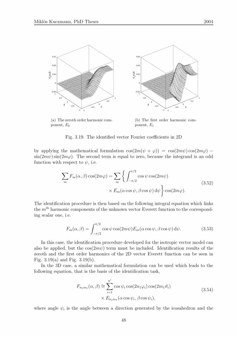
Miklos Kuczmann, PhD Theses 2004
−1
−0.5
0
0.5
1
−1
−0.5
0
0.5
1−0.04
0
0.04
0.08
0.12
αβ
E0(α
,β)
(a) The zeroth order harmonic com-ponent, E0
−1
−0.5
0
0.5
1
−1
−0.5
0
0.5
1−0.02
0
0.02
0.04
0.06
αβ
E1(α
,β)
(b) The first order harmonic com-ponent, E1
Fig. 3.19. The identified vector Fourier coefficients in 2D
by applying the mathematical formulation cos(2m(ψ + ϕ)) = cos(2mψ) cos(2mϕ) −sin(2mψ) sin(2mϕ). The second term is equal to zero, because the integrand is an oddfunction with respect to ψ, i.e.
∑
m
Fm(α, β) cos(2mϕ) =∑
m
∫ π/2
−π/2
cosψ cos(2mψ)
× Em(α cosψ, β cosψ) dψ
cos(2mϕ).
(3.52)
The identification procedure is then based on the following integral equation which linksthe mth harmonic components of the unknown vector Everett function to the correspond-ing scalar one, i.e.
Fm(α, β) =
∫ π/2
−π/2
cosψ cos(2mψ)Em(α cosψ, β cosψ) dψ. (3.53)
In this case, the identification procedure developed for the isotropic vector model canalso be applied, but the cos(2mψ) term must be included. Identification results of thezeroth and the first order harmonics of the 2D vector Everett function can be seen inFig. 3.19(a) and Fig. 3.19(b).
In the 3D case, a similar mathematical formulation can be used which leads to thefollowing equation, that is the basis of the identification task,
Fn1m1(α, β) ∼=
n′∑
i=1
cosψi cos(2n1ϕi) cos(2m1ϑi)
× En1m1(α cosψi, β cosψi),
(3.54)
where angle ψi is the angle between a direction generated by the icosahedron and the
48

Miklos Kuczmann, PhD Theses 2004
−1
−0.5
0
0.5
1
−1
−0.5
0
0.5
1−0.04
0
0.04
0.08
0.12
αβ
E00
(α,β
)
(a) The zeroth order harmonic com-ponent, E00
−1
−0.5
0
0.5
1
−1
−0.5
0
0.5
1−0.01
0
0.01
0.02
0.03
αβ
E01
(α,β
)
(b) The first order harmonic com-ponent, E01
−1
−0.5
0
0.5
1
−1
−0.5
0
0.5
1−0.02
−0.01
0
0.01
0.02
αβ
E10
(α,β
)
(c) The first order harmonic com-ponent, E10
−1
−0.5
0
0.5
1
−1
−0.5
0
0.5
1−0.02
−0.01
0
0.01
0.02
αβ
E11
(α,β
)
(d) The first order harmonic com-ponent, E11
Fig. 3.20. The identified vector Fourier coefficients in 3D
x–axis. In this case, equation (3.37) should be rewritten in a simplified form,
F (αk, βl, ϕj, ϑj) ∼=
n′∑
i=1
cosψiE(αk cosψi, βl cosψi, ϕi, ϑi), (3.55)
where n′ is replaced by n′ ·m′. The four identified Fourier series of the vector Everettfunction are plotted in Fig. 3.20(a)–3.20(d).
From the Fourier coefficients of the vector Everett function, the Everett functions inall directions (e.g. 9 directions generated by the icosahedron) as well as the first orderreversal curves can be calculated, then NNs can be trained. It is obvious that, differentNNs must be trained in different directions.
49
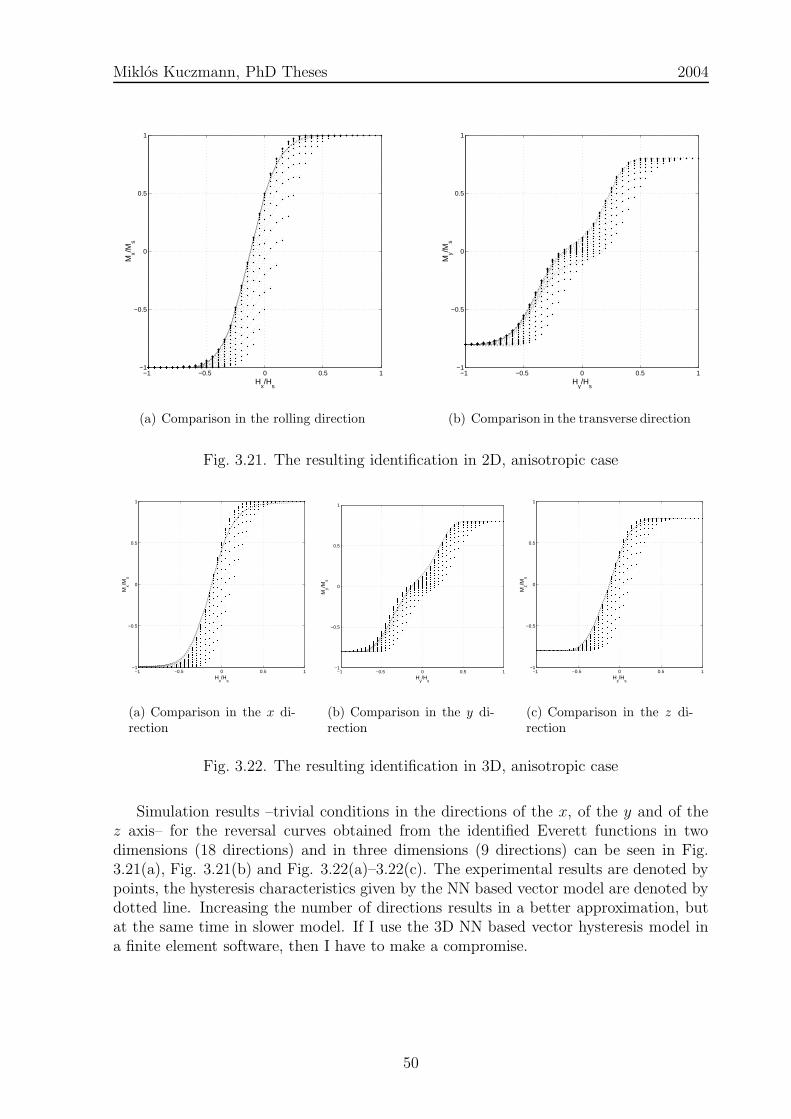
Miklos Kuczmann, PhD Theses 2004
−1 −0.5 0 0.5 1−1
−0.5
0
0.5
1
Hx/H
s
Mx/M
s
(a) Comparison in the rolling direction
−1 −0.5 0 0.5 1−1
−0.5
0
0.5
1
Hy/H
s
My/M
s
(b) Comparison in the transverse direction
Fig. 3.21. The resulting identification in 2D, anisotropic case
−1 −0.5 0 0.5 1−1
−0.5
0
0.5
1
Hx/H
s
Mx/M
s
(a) Comparison in the x di-rection
−1 −0.5 0 0.5 1−1
−0.5
0
0.5
1
Hy/H
s
My/M
s
(b) Comparison in the y di-rection
−1 −0.5 0 0.5 1−1
−0.5
0
0.5
1
Hz/H
s
Mz/M
s
(c) Comparison in the z di-rection
Fig. 3.22. The resulting identification in 3D, anisotropic case
Simulation results –trivial conditions in the directions of the x, of the y and of thez axis– for the reversal curves obtained from the identified Everett functions in twodimensions (18 directions) and in three dimensions (9 directions) can be seen in Fig.3.21(a), Fig. 3.21(b) and Fig. 3.22(a)–3.22(c). The experimental results are denoted bypoints, the hysteresis characteristics given by the NN based vector model are denoted bydotted line. Increasing the number of directions results in a better approximation, butat the same time in slower model. If I use the 3D NN based vector hysteresis model ina finite element software, then I have to make a compromise.
50
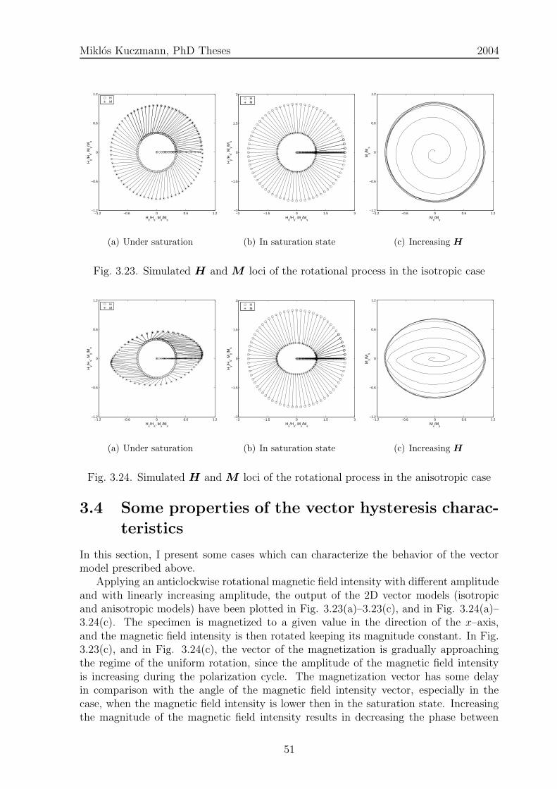
Miklos Kuczmann, PhD Theses 2004
−1.2 −0.6 0 0.6 1.2−1.2
−0.6
0
0.6
1.2
Hx/H
s, M
x/M
s
Hy/H
s, My/M
s
HM
(a) Under saturation
−3 −1.5 0 1.5 3−3
−1.5
0
1.5
3
Hx/H
s, M
x/M
s
Hy/H
s, My/M
s
HM
(b) In saturation state
−1.2 −0.6 0 0.6 1.2−1.2
−0.6
0
0.6
1.2
Mx/M
s
My/M
s
(c) Increasing H
Fig. 3.23. Simulated H and M loci of the rotational process in the isotropic case
−1.2 −0.6 0 0.6 1.2−1.2
−0.6
0
0.6
1.2
Hx/H
s, M
x/M
s
Hy/H
s, My/M
s
HM
(a) Under saturation
−3 −1.5 0 1.5 3−3
−1.5
0
1.5
3
Hx/H
s, M
x/M
s
Hy/H
s, My/M
s
HM
(b) In saturation state
−1.2 −0.6 0 0.6 1.2−1.2
−0.6
0
0.6
1.2
Mx/M
s
My/M
s
(c) Increasing H
Fig. 3.24. Simulated H and M loci of the rotational process in the anisotropic case
3.4 Some properties of the vector hysteresis charac-
teristics
In this section, I present some cases which can characterize the behavior of the vectormodel prescribed above.
Applying an anticlockwise rotational magnetic field intensity with different amplitudeand with linearly increasing amplitude, the output of the 2D vector models (isotropicand anisotropic models) have been plotted in Fig. 3.23(a)–3.23(c), and in Fig. 3.24(a)–3.24(c). The specimen is magnetized to a given value in the direction of the x–axis,and the magnetic field intensity is then rotated keeping its magnitude constant. In Fig.3.23(c), and in Fig. 3.24(c), the vector of the magnetization is gradually approachingthe regime of the uniform rotation, since the amplitude of the magnetic field intensityis increasing during the polarization cycle. The magnetization vector has some delayin comparison with the angle of the magnetic field intensity vector, especially in thecase, when the magnetic field intensity is lower then in the saturation state. Increasingthe magnitude of the magnetic field intensity results in decreasing the phase between
51

Miklos Kuczmann, PhD Theses 2004
−1.6 −0.8 0 0.8 1.6−1.6
−0.8
0
0.8
1.6
Hx/H
s, M
x/M
s
Hy/H
s, My/M
s
HM
(a) Vectors of H and M
−1.6 −0.8 0 0.8 1.6−1
−0.5
0
0.5
1
Hx/H
s
Mx/M
s
(b) The hysteresis character-istic in the x–axis
−1.6 −0.8 0 0.8 1.6−1
−0.5
0
0.5
1
Hy/H
s
My/M
s
(c) The hysteresis character-istic in the y–axis
Fig. 3.25. The simulated H and M loci of the linear excitation in the isotropic case
−1.6 −0.8 0 0.8 1.6−1.6
−0.8
0
0.8
1.6
Hx/H
s, M
x/M
s
Hy/H
s, My/M
s
HM
(a) Vectors of H and M
−1.6 −0.8 0 0.8 1.6−1
−0.5
0
0.5
1
Hx/H
s
Mx/M
s
(b) The hysteresis character-istic in the x–axis
−1.6 −0.8 0 0.8 1.6−1
−0.5
0
0.5
1
My/M
s
Hx/H
s
(c) The hysteresis character-istic in the y–axis
Fig. 3.26. The simulated H and M loci of the linear excitation in the anisotropic case
the magnetization and the magnetic field intensity vectors. Higher above the satura-tion state, they rotate together. In the figures yielded by the anisotropic model, theanisotropic behavior can be seen easily, because the amplitude of magnetization in they–axis is smaller than in the x–axis and the delay between the magnetic field intensityand magnetization vectors is larger.
In the second test case, the magnetic field intensity vector has applied in a linearvariation (ϑH = 60). In isotropic case, the magnetic field intensity and the magne-tization vectors are parallel as plotted in Fig. 3.25(a)–3.25(c), but in anisotropic case(see Fig. 3.26(a)–3.26(c)) there is an angle between them, because of the anisotropicbehavior: the magnetization vector tries to be close to the x–axis. The projected hys-teresis characteristics in the x–axis and in the y–axis are also presented. The hysteresischaracteristics in the x-axis and in the y–axis are similar in the isotropic case, but theshape of the characteristics is very different in the anisotropic case.
Anisotropic behavior of the isotropic model induced by the remanent magnetizationcan be observed as well. Let us suppose that, the magnetic field intensity is first increased
52

Miklos Kuczmann, PhD Theses 2004
0 0.3 0.6 0.9 1.20
0.3
0.6
0.9
1.2
Hx/H
s, M
x/M
s
Hy/H
s, My/M
s
HM
(a) 2D model
0
0.3
0.6
0.9
1.2
0
0.3
0.6
0.9
1.2
0
0.3
0.6
0.9
1.2
Hx/H
s, M
x/M
s
Hy/H
s, M
y/M
s
Hz/H
s, Mz/M
s
HM
(b) 3D model
Fig. 3.27. The induced anisotropy in isotropic material
in the y direction to a given value, and then it is decreased to zero. This process results ina remanent magnetization in the y direction. After reaching the remanent magnetization,the magnetic field intensity is increased in the x direction. The orthogonal remanentmagnetization can be reduced as presented in the Fig. 3.27(a). In the 3D case, a similarmagnetization process can be applied with similar simulation results, e.g. the magneticfield intensity is increased and then decreased in the x direction resulting remanentmagnetization in the x direction, then increased and then decreased in the z direction,and finally increased in the y direction. This process can be seen in Fig. 3.27(b).
Using a large number of directions results better approximation, but the calcula-tions may be time consuming. Smaller number of directions gives higher error betweenmeasured and simulated curves, however the model is faster. To make a compromise,the presented model with given number of directions can be used in Computer AidedDesign software tools (e.g. in the Finite Element Method) with a given accuracy whichis acceptable as illustrated in the figures of this chapter.
3.5 New scientific results
1. Thesis I have developed a new scalar hysteresis operator based on the function ap-proximation capability of the neural networks to simulate the behavior of ferromagneticmaterials. I have represented the first order reversal curves with a surface by introduc-ing the variable ξ and I have approximated this surface by neural network technique.I have built a knowledge–base which contains if–then type rules about the behavior ofthe hysteresis characteristics. I have shown the applicability of the model by comparingsimulated and measured results. I have taken into account the vectorial behavior of themagnetic field intensity and the magnetic flux density by applying the neural networkbased vector hysteresis model, and I have recommended a new identification procedureto build up the vector model. I have worked out the three dimensional anisotropic vector
53

Miklos Kuczmann, PhD Theses 2004
hysteresis model, and I have analyzed the behavior of the developed vector models.
1.a I have developed a new neural network based mathematical representation of thescalar hysteresis operator. I have handled the multivalued property of the hysteresischaracteristics by introducing the new variable ξ associated with the measured firstorder reversal curves. This preprocessing can be applied on any kind of hysteresischaracteristics. I have built a knowledge–base which contains if–then type rulesabout the behavior of the hysteresis characteristics. This is the memory mechanismof the model. I have realized the identification procedure by the training of theneural networks. I have built a measurement system to measure hysteresis curveson a toroidal shape C19 structural steel, and I have used these measurementsto show the applicability of the neural network based scalar hysteresis model bycomparing measurements and simulation results.
1.b I have developed the two dimensional and the three dimensional isotropic vectorhysteresis models based on the neural network based scalar model. I have workedout an original and new identification procedure based on the measurable Everettfunction both to predict two dimensional and three dimensional isotropic hysteresischaracteristics. I have compared the measured and the predicted curves and I haveshown the behavior of the vector model in linear and in rotational magnetic fields.
1.c I have developed the two dimensional and the three dimensional neural networkbased anisotropic vector hysteresis models by the means of Fourier expansion ofthe measured Everett function of the anisotropic material. I have generalized thetwo dimensional model in three dimensions as a theoretical expansion of the twodimensional model, and I have recommended an identification procedure to fit tomeasured curves. I have compared the measured and the predicted curves and Ihave shown the behavior of the vector model in linear and in rotational magneticfields, finally I have compared the isotropic and the anisotropic models.
54
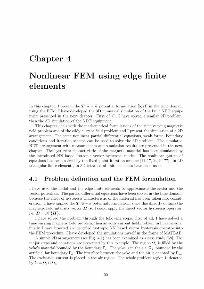
Chapter 4
Nonlinear FEM using edge finite
elements
In this chapter, I present the T ,Ψ− Ψ potential formulation [6, 21] in the time domainusing the FEM. I have developed the 3D numerical simulation of the built NDT equip-ment presented in the next chapter. First of all, I have solved a similar 2D problem,then the 3D simulation of the NDT equipment.
This chapter deals with the mathematical formulations of the time varying magneticfield problem and of the eddy current field problem and I present the simulation of a 2Darrangement. The same nonlinear partial differential equations, weak forms, boundaryconditions and iteration scheme can be used to solve the 3D problem. The simulatedNDT arrangement with measurements and simulation results are presented in the nextchapter. The hysteresis characteristic of the magnetic material has been simulated bythe introduced NN based isotropic vector hysteresis model. The nonlinear system ofequations has been solved by the fixed–point iteration scheme [11, 17, 24, 49, 77]. In 2Dtriangular finite elements, in 3D tetrahedral finite elements have been used.
4.1 Problem definition and the FEM formulation
I have used the nodal and the edge finite elements to approximate the scalar and thevector potentials. The partial differential equations have been solved in the time domain,because the effect of hysteresis characteristic of the material has been taken into consid-eration. I have applied the T ,Ψ−Ψ potential formulation, since this directly obtains themagnetic field intensity vector H, so I could apply the direct vector hysteresis operator,i.e. B = H H.
I have solved the problem through the following steps: first of all, I have solved atime varying magnetic field problem, then an eddy current field problem in linear media,finally I have inserted an identified isotropic NN based vector hysteresis operator intothe FEM procedure. I have developed the simulations myself in the frame of MATLAB.
A simple 2D arrangement (see Fig. 4.1) has been examined as a case study [58]. Themajor steps and equations are presented by this example. The region Ωc is filled by theyoke’s material bounded by the boundary Γc. The yoke is in the air, Ωn, bounded by theartificial far boundary Γn. The interface between the yoke and the air is denoted by Γnc.The excitation current is placed in the air region. The whole problem region is denotedby Ω = Ωc ∪ Ωn.
55

Miklos Kuczmann, PhD Theses 2004
PSfrag replacements
x
y
symmetry plane
air
iron
coil
Ωn
Γn
Ωc
ΓcΓc
Γnc
Fig. 4.1. Sketch of the solved 2D problem, a case study
−100 −50 0 50 1000
25
50
75
100
x[mm]
y[m
m]
(a) The generated FEMmesh
−100 −50 0 50 100 0
25
50
75
100
x [mm]
y [m
m]
(b) The generated edges
−100 −50 0 50 100 0
25
50
75
100
x [mm]
y [m
m]
Ψ=0
T=0
(c) The applied boundaryconditions( : Ψ = 0,→: T = 0, presented inthe text)
Fig. 4.2. The generated mesh of the 2D problem
The example contains a closed yoke made of iron with excitation coils under a givenwaveform of current. First, the characteristic of the yoke is linear, then the hysteresischaracteristic of the yoke’s material has been taken into consideration. Only the half ofthe arrangement has been analyzed, because this is symmetrical with respect to the liney = 0. The generated FEM mesh has been finalized after some preliminary simulations,and it contains 299 nodes, 548 finite elements (Fig. 4.2(a), the size of the arrangementalso can be seen in this figure) and 846 edges (Fig. 4.2(b)). The generated mesh is aDelaunay–type mesh. The applied boundary conditions can be seen in Fig. 4.2(c) [6,21]and presented below in the text.
4.1.1 Time varying magnetic field problem in linear media
As the simplest case, the closed yoke made of linear magnetic material with a givenrelative permeability µr is placed into air. The excitation is a coil wounded around theyoke with sinusoidal time function of current i(t).
56
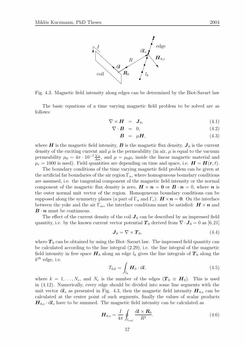
Miklos Kuczmann, PhD Theses 2004PSfrag replacements
dl
R
R0
H0,s
I
lk
dls
coil
edge
Fig. 4.3. Magnetic field intensity along edges can be determined by the Biot-Savart law
The basic equations of a time varying magnetic field problem to be solved are asfollows:
∇×H = J0, (4.1)
∇ ·B = 0, (4.2)
B = µH, (4.3)
where H is the magnetic field intensity, B is the magnetic flux density, J 0 is the currentdensity of the exciting current and µ is the permeability (in air, µ is equal to the vacuumpermeability µ0 = 4π · 10−7 V s
Am, and µ = µ0µr inside the linear magnetic material and
µr = 1000 is used). Field quantities are depending on time and space, i.e. H = H(r, t).The boundary conditions of the time varying magnetic field problem can be given at
the artificial far boundaries of the air region Γn, where homogeneous boundary conditionsare assumed, i.e. the tangential component of the magnetic field intensity or the normalcomponent of the magnetic flux density is zero, H × n = 0 or B · n = 0, where n isthe outer normal unit vector of the region. Homogeneous boundary conditions can besupposed along the symmetry planes (a part of Γn and Γc): H×n = 0. On the interfacebetween the yoke and the air Γnc, the interface conditions must be satisfied: H ×n andB · n must be continuous.
The effect of the current density of the coil J 0 can be described by an impressed fieldquantity, i.e. by the known current vector potential T 0 derived from ∇·J0 = 0 as [6,21]
J0 = ∇× T 0, (4.4)
where T 0 can be obtained by using the Biot–Savart law. The impressed field quantity canbe calculated according to the line integral (2.29), i.e. the line integral of the magneticfield intensity in free space H0 along an edge lk gives the line integrals of T 0 along thekth edge, i.e.
T0,k =
∫
lk
H0 · dl, (4.5)
where k = 1, . . . , Ne, and Ne is the number of the edges (T 0 ≡ H0). This is usedin (4.12). Numerically, every edge should be divided into some line segments with theunit vector dls as presented in Fig. 4.3, then the magnetic field intensity H0,s can becalculated at the center point of such segments, finally the values of scalar productsH0,s · dls have to be summed. The magnetic field intensity can be calculated as
H0,s =I
4π
∮
lcoil
dl×R0
R2. (4.6)
57
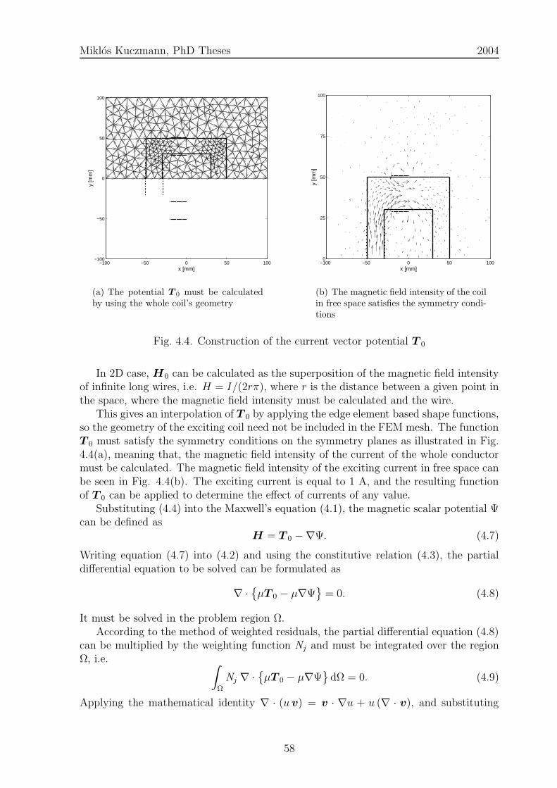
Miklos Kuczmann, PhD Theses 2004
−100 −50 0 50 100−100
−50
0
50
100
x [mm]
y [m
m]
(a) The potential T 0 must be calculatedby using the whole coil’s geometry
−100 −50 0 50 1000
25
50
75
100
x [mm]
y [m
m]
(b) The magnetic field intensity of the coilin free space satisfies the symmetry condi-tions
Fig. 4.4. Construction of the current vector potential T 0
In 2D case, H0 can be calculated as the superposition of the magnetic field intensityof infinite long wires, i.e. H = I/(2rπ), where r is the distance between a given point inthe space, where the magnetic field intensity must be calculated and the wire.
This gives an interpolation of T 0 by applying the edge element based shape functions,so the geometry of the exciting coil need not be included in the FEM mesh. The functionT 0 must satisfy the symmetry conditions on the symmetry planes as illustrated in Fig.4.4(a), meaning that, the magnetic field intensity of the current of the whole conductormust be calculated. The magnetic field intensity of the exciting current in free space canbe seen in Fig. 4.4(b). The exciting current is equal to 1 A, and the resulting functionof T 0 can be applied to determine the effect of currents of any value.
Substituting (4.4) into the Maxwell’s equation (4.1), the magnetic scalar potential Ψcan be defined as
H = T 0 −∇Ψ. (4.7)
Writing equation (4.7) into (4.2) and using the constitutive relation (4.3), the partialdifferential equation to be solved can be formulated as
∇ ·µT 0 − µ∇Ψ
= 0. (4.8)
It must be solved in the problem region Ω.According to the method of weighted residuals, the partial differential equation (4.8)
can be multiplied by the weighting function Nj and must be integrated over the regionΩ, i.e. ∫
Ω
Nj ∇ ·µT 0 − µ∇Ψ
dΩ = 0. (4.9)
Applying the mathematical identity ∇ · (u v) = v · ∇u + u (∇ · v), and substituting
58
Miklos Kuczmann, PhD Theses 2004
u = Nj and v = µT 0 − µ∇Ψ, and using the Gauss law, leads to the equation
−
∫
Ω
∇Nj ·µT 0 − µ∇Ψ
dΩ +
∮
Γ
Nj
µT 0 − µ∇Ψ
· n dΓ = 0. (4.10)
The boundary integral term is equal to zero, because B · n = 0 on the artificial farboundary Γn, so the equation for one finite element is the following:
µ
∫
Ωe
∇Nj · ∇Ψ dΩ = µ
∫
Ωe
∇Nj · T 0 dΩ, (4.11)
where Ωe represents one finite element. In the case of FEM, the weighting function Nj
is equal to the basis function of the nodal FEM.The unknown magnetic scalar potential Ψ is approximated by linear nodal basis
functions Ni, the known current vector potential T 0 is approximated by linear edgebasis functions W k as
Ψ 'I∑
i=1
Ni Ψi, T 0 'K∑
k=1
W k T0,k. (4.12)
The number of degrees of freedom is I = 3, and K = 3 using triangular finite elements.For simplicity, the subscript h presented in sections 2.5.1 and 2.5.2 is omitted.
Substituting the approximation functions (4.12) into the weak formulation (4.11),the system of equations of one finite element can be derived as
I∑
i=1
µ
∫
Ωe
∇Nj · ∇Ni dΩ
Ψi =
K∑
k=1
µ
∫
Ωe
∇Nj ·W k dΩ
T0,k. (4.13)
This system of equation contains I equations and j = 1, . . . , I. After assembling thissystem of equations, a system of equations (stored by using the sparse technique) can beobtained which contains as many unknowns as the number of nodes of the finite elementmesh.
The magnetic scalar potential along the artificial boundary and along the symmetryplane is set to be zero. By using the nodal shape functions to approximate the unknownmagnetic scalar potential, the interface conditions can be fulfilled automatically. Thesolution of this assembled system of equation gives the approximation of the unknownmagnetic scalar potential Ψ.
Simulation results as comparisons with the results of the eddy current field problemare presented in the next section.
4.1.2 Eddy current field in linear media
The same closed iron yoke made of linear and conducting magnetic material with relativepermeability µr and conductivity σ is placed into air (µr = 1000 and σ = 1/48·108 S/m).The excitation is the current flowing in the coil with sinusoidal function i(t). The dis-placement current ∂D/∂t is neglected. In time–varying case, electric and magnetic fields
59
Miklos Kuczmann, PhD Theses 2004
are coupled as described by Maxwell’s equations
∇×H = J0 + J e ≡ J , (4.14)
∇×E = −B, (4.15)
∇ ·B = 0, (4.16)
B = µH, (4.17)
J = σE, (4.18)
where H and E are the magnetic and the electric field intensities, B is the magnetic fluxdensity, J0 is the current density of the excitation coils, and J is the current density equalto J0 in air, but contains the effect of the eddy currents J e in the conducting material.Symbol µ is the permeability and σ is the conductivity of the magnetic material, · denotesthe time derivative.
The boundary conditions of the eddy current field problem can be given as follows. Atthe artificial far boundaries of the nonconducting region (air) Γn, homogeneous boundaryconditions are assumed, i.e. the tangential component of the magnetic field intensity orthe normal component of the magnetic flux density is zero, H×n = 0 or B ·n = 0, wheren is the outer normal unit vector of the region. Homogeneous boundary conditions canbe supposed along the symmetry planes (a part of Γn and Γc): H×n = 0, i.e. J ·n = 0and E × n = 0. On the interface between the conducting (yoke) and nonconducting(air) regions Γnc, the interface conditions must be satisfied: H × n and B · n must becontinuous and J · n = 0.
Starting from ∇ · J = 0, the current density J can be described by two currentvector potentials [6,21]: one is the known current vector potential T 0, corresponding tothe exciting current, the other is the unknown current vector potential T , defined onlyin the conducting material, Ωc, taking into account the effect of the eddy currents, i.e.
J ≡ J0 + J e = ∇× T 0 +∇× T , (4.19)
that is J0 = ∇× T 0 and J e = ∇× T . The magnetic field intensity H can be approx-imated by the magnetic scalar potential Ψ and by the current vector potentials T andT 0 by substituting equation (4.19) into (4.14), i.e.
H =
T 0 −∇Ψ, in air containing the coil,T 0 + T −∇Ψ, in conducting material.
(4.20)
The problem can be divided into two parts: there is a time varying magnetic field problemin air, and an eddy current field problem in the conducting material. The two parts mustbe coupled. This is the so called T ,Ψ− Ψ potential formulation.
Substituting (4.19) into the relation (4.18) and using the characteristic (4.17) and thesecond definition in (4.20), Maxwell’s equation (4.15) can be formulated by the partialdifferential equation
∇×1
σ∇× T + µT − µ∇Ψ = −∇×
1
σ∇× T 0 − µT 0. (4.21)
The Maxwell’s equation (4.16) can be rewritten in the form
∇ ·µT 0 + µT − µ∇Ψ
= 0. (4.22)
60
Miklos Kuczmann, PhD Theses 2004
The partial differential equations to be solved in this case are the equation (4.8) in air(but µ = µ0), moreover the equations (4.21) and (4.22) in the conducting material.These equations are coupled through the interface conditions between the air and theconducting material.
According to the method of weighted residuals, the partial differential equation (4.21)can be multiplied by the vector weighting function W j and integrated over the regionΩ, i.e.
∫
Ω
W j · ∇ ×1
σ∇× T dΩ +
∫
Ω
µW j · T dΩ−
∫
Ω
µW j · ∇Ψ dΩ
= −
∫
Ω
W j · ∇ ×1
σ∇× T 0 dΩ−
∫
Ω
µW j · T 0 dΩ.
(4.23)
Applying the mathematical identity ∇· (u×v) = v ·∇×u−u ·∇×v, and substitutingu = W j and v = 1
σ∇ × T , and using the Gauss law, the following equation can be
obtained:∫
Ω
1
σ∇×W j · ∇ × T dΩ−
∮
Γ
W j ×
(1
σ∇× T
)· ndΓ
+
∫
Ω
µW j · T dΩ−
∫
Ω
µW j · ∇Ψ dΩ
= −
∫
Ω
1
σ∇×W j · ∇ × T 0 dΩ +
∮
Γ
W j ×
(1
σ∇× T 0
)· n dΓ
−
∫
Ω
µW j · T 0 dΩ.
(4.24)
The boundary integral terms can be neglected, because E × n = 0 at the boundary ofthe conducting material Γc, i.e.
∫
Ω
1
σ∇×W j · ∇ × T dΩ +
∫
Ω
µW j · T dΩ−
∫
Ω
µW j · ∇Ψ dΩ
= −
∫
Ω
1
σ∇×W j · ∇ × T 0 dΩ−
∫
Ω
µW j · T 0 dΩ.
(4.25)
The approximating functions can also be introduced as the weighted sum of the potentialvalues in nodes and along edges, i.e.
Ψ '
I∑
i=1
Ni Ψi, T 0 '
K∑
k=1
W k T0,k, T '
K∑
k=1
W k Tk. (4.26)
The number of degrees of freedom is I +K = 6 using triangular finite elements.The time derivatives of the variables have been approximated by the Euler backward
algorithm, T ' T(n+1)−T
(n)
∆tnat a given discrete time of the simulation tn. Using this
formula and substituting equations in (4.26) into (4.25), then the following system of
61
Miklos Kuczmann, PhD Theses 2004
equations can be obtained in one finite element placed in the conducting material:
K∑
k=1
1
σ
∫
Ωe
∇×W j · ∇ ×W k dΩ +µ
4t
∫
Ωe
W j ·W k dΩ
T
(n+1)k
−
I∑
i=1
µ
4t
∫
Ωe
W j · ∇Ni dΩ
Ψ
(n+1)i
=K∑
k=1
µ
4t
∫
Ωe
W j ·W k dΩ
T
(n)k −
I∑
i=1
µ
4t
∫
Ωe
W j · ∇Ni dΩ
Ψ
(n)i
−
K∑
k=1
1
σ
∫
Ωe
∇×W j · ∇ ×W k dΩ
T
(n+1)0,k
−K∑
k=1
µ
4t
∫
Ωe
W j ·W k dΩ
T
(n+1)0,k − T
(n)0,k
.
(4.27)
The partial differential equation (4.22), similarly as in the time varying magnetic fieldproblem, can be weighted by the scalar weighting function Nj and must be integratedover the region Ω, i.e.
∫
Ω
Nj ∇ ·µT 0 + µT − µ∇Ψ
dΩ = 0. (4.28)
Applying similar mathematical formulations as in the time varying magnetic field prob-lem, the following system of linear equations can be obtained in one finite element:
−
K∑
k=1
µ
∫
Ωe
∇Nj ·W k dΩ
T
(n+1)k +
I∑
i=1
µ
∫
Ωe
∇Nj · ∇Ni dΩ
Ψ
(n+1)i
=K∑
k=1
µ
∫
Ωe
∇Nj ·W k dΩ
T
(n+1)0,k .
(4.29)
The boundary conditions are the following: the magnetic scalar potential along theboundary and the symmetry plane as well as the tangential component of the unknowncurrent vector potential along the symmetry plane and along the interface between theconducting and the nonconducting material are set to be zero.
Unfortunately, the system of linear equations generated by the edge elements of theFEM is singular which can only be solved by iterative solvers. I used the stabilized bicon-jugate gradient method (bicgstab, implemented in MATLAB [26,99]). This iterativelyfinds an accurate solution of the system of equations starting from an initial guess. Thesolution is depending on the starting vector. The stopping criterion is based on the error
ε =‖b−Kx‖
‖b‖(4.30)
to reach ε < 10−12, and K is the system matrix, b is the right hand side of the assembledequations and x contains the unknown potentials. The initial guess of the iteration at atime instant is the stable solution of the previous time instant.
62

Miklos Kuczmann, PhD Theses 2004
−100 −50 0 50 100 0
25
50
75
100
x [mm]
y [m
m]
(a) The magnetic field intensity, H
−100 −50 0 50 100 0
25
50
75
100
x [mm]
y [m
m]
(b) The magnetic flux density, B
Fig. 4.5. Results of the time varying magnetic field simulations
−100 −50 0 50 100 0
25
50
75
100
x [mm]
y [m
m]
(a) The magnetic field intensity, H
−100 −50 0 50 100 0
25
50
75
100
x [mm]
y [m
m]
(b) The magnetic flux density, B
Fig. 4.6. Results of the eddy current field simulations, f = 2 Hz
The solution of the resulting system of linear equations gives the unknown potentialsT and Ψ at the time instant tn+1.
The test example has been studied with the following parameters: the eddy currentfield problem in linear media has been run for four periods to reach the stationary state,one period has been divided into 40 time steps and the peak value and the frequency ofthe exciting current have been 1 A and 2 Hz, respectively. The following figures comparethe results of the time varying magnetic field problem and the results of the eddy currentfield problem. The vectors of the magnetic field intensity and of the magnetic flux densitycan be seen in Fig. 4.5(a) and Fig. 4.5(b), and in Fig. 4.6(a) and Fig. 4.6(b) for the time
63

Miklos Kuczmann, PhD Theses 2004
30 35 40 45 50−500
−250
0
250
500
y [mm]
Hx [A
/m]
(a) f = 0.1 Hz, δ ' 35 mm
30 35 40 45 50−500
−250
0
250
500
y [mm]
Hx [A
/m] δ
Lδ
R
(b) f = 1 Hz, δ ' 11 mm
30 35 40 45 50−500
−250
0
250
500
y [mm]
Hx [A
/m]
δL
δR
(c) f = 10 Hz, δ ' 3.5 mm
30 35 40 45 50−500
−250
0
250
500
y [mm]
Hx [A
/m]
δL
δR
(d) f = 100 Hz, δ ' 1.1 mm
Fig. 4.7. The effect of extrusion of current v.s. increasing the frequency
varying case and for the eddy current case, respectively. The figures show the vectors atthe time instant, when the current has a maximum value. The effect of the eddy currentsis unambiguous in the pictures, let us compare the figures: the value of H and of B aresmaller inside the magnetic material in the case of the eddy current field problem thanin the case of the time varying magnetic field problem. This effect can be associatedwith the skin effect. The effect of frequency of the exciting current can be seen in Fig.4.7(a)–4.7(d). These figures illustrate the x component of the magnetic field intensityHx inside the yoke, along the line x = 20 mm, and y ∈ [30, . . . , 50] mm. The value of
the skin depth has been calculated by δ = δL = δR =√
1πfµσ
. Applying linear shape
functions results in staircase like functions as can be seen in the figures.
64
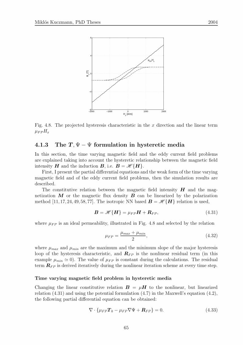
Miklos Kuczmann, PhD Theses 2004
−2000 −1000 0 1000 2000−8
−4
0
4
8
Hx [A/m]
Bx [T
]
µFP
Hx
Fig. 4.8. The projected hysteresis characteristic in the x direction and the linear termµFPHx
4.1.3 The T ,Ψ−Ψ formulation in hysteretic media
In this section, the time varying magnetic field and the eddy current field problemsare explained taking into account the hysteretic relationship between the magnetic fieldintensity H and the induction B, i.e. B = H H.
First, I present the partial differential equations and the weak form of the time varyingmagnetic field and of the eddy current field problems, then the simulation results aredescribed.
The constitutive relation between the magnetic field intensity H and the mag-netization M or the magnetic flux density B can be linearized by the polarizationmethod [11, 17, 24, 49, 58, 77]. The isotropic NN based B = H H relation is used,
B = H H = µFPH + RFP , (4.31)
where µFP is an ideal permeability, illustrated in Fig. 4.8 and selected by the relation
µFP =µmax + µmin
2, (4.32)
where µmax and µmin are the maximum and the minimum slope of the major hysteresisloop of the hysteresis characteristic, and RFP is the nonlinear residual term (in thisexample µmin ' 0). The value of µFP is constant during the calculations. The residualterm RFP is derived iteratively during the nonlinear iteration scheme at every time step.
Time varying magnetic field problem in hysteretic media
Changing the linear constitutive relation B = µH to the nonlinear, but linearizedrelation (4.31) and using the potential formulation (4.7) in the Maxwell’s equation (4.2),the following partial differential equation can be obtained:
∇ · µFPT 0 − µFP∇Ψ + RFP = 0. (4.33)
65
Miklos Kuczmann, PhD Theses 2004
This equation is valid in the magnetic material Ωc. The partial differential equationin the air region Ωn is (4.8), but µ = µ0. The boundary conditions are the same asprescribed in section 4.1.1.
Applying the method of weighted residuals, the following system of equations for onefinite element can be obtained in the nonlinear medium:
I∑
i=1
µFP
∫
Ωe
∇Nj · ∇Ni dΩ
Ψi
=
K∑
k=1
µFP
∫
Ωe
∇Nj ·W k dΩ
T0,k +
∫
Ωe
∇Nj ·RFP dΩ.
(4.34)
This system of equations is coupled with the weak form (4.13) with µ = µ0.Only one NN based hysteresis operator is defined in the barycenter of one finite
element, therefore the nonlinear residual term RFP is supposed to be constant in a finiteelement.
Eddy current field problem in hysteretic media
Using the linearized constitutive relation (4.31) in nonlinear media, Ωc, and the secondpotential formulation in (4.20) in the Maxwell’s equations (4.15) and (4.16) with therelation (4.18) leads to the following partial differential equations:
∇×1
σ∇× T + µFP T − µFP∇Ψ = −∇×
1
σ∇× T 0 − µFP T 0 − RFP , (4.35)
∇ · µFPT 0 + µFPT − µFP∇Ψ + RFP = 0. (4.36)
The partial differential equation (4.8) valid in the air region Ωn with µ = µ0 must becoupled with the above partial differential equations (4.35) and (4.36) applying the sameboundary conditions as prescribed in section 4.1.2.
After using the method of weighted residuals and the Euler backward algorithm, thefollowing system of linear equations can be obtained for one finite element from thepartial differential equations (4.35) and (4.36):
K∑
k=1
1
σ
∫
Ωe
∇×W j · ∇ ×W k dΩ +µFP4t
∫
Ωe
W j ·W k dΩ
T
(n+1)k
−
I∑
i=1
µFP4t
∫
Ωe
W j · ∇Ni dΩ
Ψ
(n+1)i
=K∑
k=1
µFP4t
∫
Ωe
W j ·W k dΩ
T
(n)k −
I∑
i=1
µFP4t
∫
Ωe
W j · ∇Ni dΩ
Ψ
(n)i
−
K∑
k=1
1
σ
∫
Ωe
∇×W j · ∇ ×W k dΩ
T
(n+1)0,k
−K∑
k=1
µFP4t
∫
Ωe
W j ·W k dΩ
T
(n+1)0,k − T
(n)0,k
−1
4t
∫
Ωe
W j ·R
(n)FP −R
(n−1)FP
dΩ,
(4.37)
66
Miklos Kuczmann, PhD Theses 2004
and
−
K∑
k=1
µFP
∫
Ωe
∇Nj ·W k dΩ
T
(n+1)k +
I∑
i=1
µFP
∫
Ωe
∇Nj · ∇Ni dΩ
Ψ
(n+1)i
=K∑
k=1
µFP
∫
Ωe
∇Nj ·W k dΩ
T
(n+1)0,k +
∫
Ωe
∇Nj ·R(n)FP dΩ.
(4.38)
The fixed–point iteration method
Handling the nonlinearity of the hysteresis characteristics can be worked out by thepolarization method. An iterative solution of the governing system of linear equationsleads to an approximate solution of the time varying magnetic field and of the eddycurrent field problems at the time instant tn [11, 17, 24, 49, 58, 77].
The initial conditions (when t0 = 0) are as follows: the magnetic field intensity, themagnetic flux density and the residual term are set to be zero in all finite elements, i.e.H = 0, B = 0, RFP = 0. This is the demagnetized state of the magnetic material.
During the fixed–point iteration, the time does not change, so for simplicity, super-script n does not label. The steps of the jth fixed–point iteration step are illustrated inFig. 4.9 and are the following:
1. Generating and solving the actual –above described– system of linear equations(Kxj = bj, where K is the constant system matrix, bj is the right hand side ofthe assembled equations and the vector xj contains the unknown potentials, i.e.xj = [Tj Ψj]
T ) which gives the new iteration of the potentials Ψj and/or T j.
2. The actual value of the magnetic field intensity H j inside the magnetic material canbe calculated by the equation (4.7) or by the second expression in (4.20) accordingto the time varying magnetic field or the eddy current field problem. The value ofvector Hj is calculated only in the barycenter of all finite elements.
3. An under relaxation method has been applied to speed up the convergence of theiteration,
Hj ← (1− α)Hj−1 + αHj,
where α = 0.5j. It generates an always convergent method [65].
4. The value of the magnetic flux density vector of all finite elements Bj can beobtained by the NN based vector hysteresis operator according to the vector H j.These Hj − Bj pairs are stored. Only one vector hysteresis operator has beenapplied in one finite element, and the residual term is supposed to be constantover it.
5. Updating the residual term RFPj+1in every finite element placed in the magnetic
material,RFPj+1
= Bj − µFPHj.
6. Convergence can be controlled by the norm
ε = ‖Hj −Hj−1‖.
67

Miklos Kuczmann, PhD Theses 2004
PSfrag replacements
Initialization (demagnetized state):
t0 = 0, T 0 = 0, T = 0, Ψ = 0,M = 0, B = 0, µFP , RFP = 0,
Assembling the system matrix K
tn+1 = tn +4tn, T 0
Assembling the vector bj
Solving the equation Kxj = bj
xj → T j, Ψj
Hj = T 0 + T j −∇Ψj
Bj = H Hj
RFPj+1= Bj − µFPHj
ε = ‖Hj −Hj−1‖
Convergence?no
yes
Fix
ed–p
oint
iter
atio
n
j = 0
j = 0
j ← j + 1
Under relaxation
Fig. 4.9. Block diagram of the fixed–point iteration scheme
68

Miklos Kuczmann, PhD Theses 2004
20 30 40 50 6020
30
40
50
60
x [mm]
y [m
m]
(a) The magnetic field intensity, H
20 30 40 50 6020
30
40
50
60
x [mm]
y [m
m]
(b) The magnetic flux density, B
Fig. 4.10. Results of the nonlinear time varying magnetic field simulations
20 30 40 50 6020
30
40
50
60
x [mm]
y [m
m]
(a) The magnetic field intensity, H
20 30 40 50 6020
30
40
50
60
x [mm]
y [m
m]
(b) The magnetic flux density, B
Fig. 4.11. Results of the nonlinear eddy current field simulations, f = 1 Hz
If it is fulfilled in every finite element, then the iteration step is convergent (in myexperiments ε = 10−4 has been used after some trials). In this case, the new timeinstant can be applied (tn+1 = tn + ∆t, and j = 0), otherwise the iteration mustbe repeated from the 1st step (j ← j + 1). The new iteration step uses the new,updated residual term.
Iteration has no physical meaning, i.e. every iteration step must be started from theprevious stable point on the hysteresis characteristic and R
(n−1)FP does not change, but
R(n)FP = R
(j+1)FP .
69

Miklos Kuczmann, PhD Theses 2004
−1200 −600 0 600 1200 −1.6
−0.8
0
0.8
1.6
Hx [A/m]
Bx [T
]
H−Bs
H−Be
(a) Point 1, hysteresis curveHx −Bx
−1200 −600 0 600 1200 −1.6
−0.8
0
0.8
1.6
Hy [A/m]
By [T
]
H−Bs
H−Be
(b) Point 1, hysteresis curveHy −By
−1200 −600 0 600 1200 −1.6
−0.8
0
0.8
1.6
Hx [A/m]
Bx [T
]
H−Bs
H−Be
(c) Point 2, hysteresis curveHx −Bx
−1200 −600 0 600 1200 −1.6
−0.8
0
0.8
1.6
Hy [A/m]
By [T
]
H−Bs
H−Be
(d) Point 2, hysteresis curveHy −By
−1200 −600 0 600 1200 −1.6
−0.8
0
0.8
1.6
Hx [A/m]
Bx [T
]
H−Bs
H−Be
(e) Point 3, hysteresis curveHx −Bx
−1200 −600 0 600 1200 −1.6
−0.8
0
0.8
1.6
Hy [A/m]
By [T
]
H−Bs
H−Be
(f) Point 3, hysteresis curveHy −By
Fig. 4.12. Comparison of the projected hysteresis characteristics in the x and y directionsobtained from the time varying magnetic field (s) and eddy current field (e) problems
70
Miklos Kuczmann, PhD Theses 2004
The 2D nonlinear time varying magnetic field and the eddy current field problemshave been applied to study the fixed–point technique in the FEM. The steady state ofthe eddy current field problem can be reached after the second period of the excitation,but four periods has been calculated. The magnetic field intensity and the magneticflux density vectors are plotted in Fig. 4.10(a), Fig. 4.10(b) and in Fig. 4.11(a), Fig.
4.11(b) at the steady state when the exciting current has a maximum value (I = 5 A).The effect of eddy currents inside the magnetic material is unambiguous in the figures:the magnetic field intensity and the magnetic flux density inside the magnetic materialare smaller in the case of the eddy current field problem than in the case of the timevarying magnetic field problem. The figures show only the corner of the magnetic yoke.
I have worked out an other comparison between the time varying magnetic field andthe eddy current field problems: the projected hysteresis characteristics in the x and inthe y directions resulting by the orthogonal components of the magnetic field intensityand of the magnetic flux density have been analyzed. Three points have been selected;Point 1 is at the vertical left leg of the yoke, where the magnetic field intensity has onlyvertical, y directed component, Point 2 is at the center of the horizontal part, wherethe magnetic field intensity has only horizontal, x directed component and Point 3 is atthe corner. Results are plotted in Fig. 4.12(a)–4.12(f). The result of skin effect can beseen easily in the figures: the amplitude of the magnetic field intensity is smaller wheneddy currents are taken into account than in the time varying magnetic field problem.Hysteresis characteristics projected in the x and in the y directions are plotted at thesteady state. In the case of eddy current field problem, the hysteresis curves are smaller,since the magnetic field intensity is smaller according to the skin effect.
4.2 Summary
This 2D example shows the applicability of the T ,Ψ − Ψ potential formulation withtaking into account the hysteresis characteristic of the magnetic material in the frameof the FEM using nodal and edge shape functions.
The same formulations can be used to solve the nonlinear 3D simulation of themeasuring test equipment introduced in the next chapter.
4.3 New scientific results
2. Thesis I have implemented the developed neural network based vector hysteresismodel to the finite element method. I have applied the Ψ and the T ,Ψ − Ψ potentialformulations, because these directly give the magnetic field intensity vector which isthe input variable of the direct vector hysteresis model. I have used the nodal and theedge shape functions for the approximation of the potentials. I have handled the neuralnetwork based vector hysteresis model by applying the B–scheme of the polarizationmethod, and I have solved the linearized system of equations by the fixed–point iterationtechnique. I have used an under–relaxation scheme to speed up the convergence of themethod. This results in a convergent and a well applicable method to solve both timevarying magnetic field problem and eddy current field problem.
71
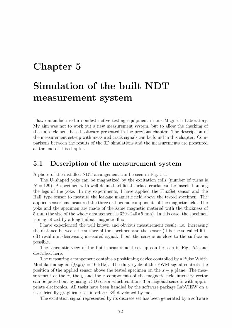
Chapter 5
Simulation of the built NDT
measurement system
I have manufactured a nondestructive testing equipment in our Magnetic Laboratory.My aim was not to work out a new measurement system, but to allow the checking ofthe finite element based software presented in the previous chapter. The description ofthe measurement set–up with measured crack signals can be found in this chapter. Com-parisons between the results of the 3D simulations and the measurements are presentedat the end of this chapter.
5.1 Description of the measurement system
A photo of the installed NDT arrangement can be seen in Fig. 5.1.The U–shaped yoke can be magnetized by the excitation coils (number of turns is
N = 129). A specimen with well defined artificial surface cracks can be inserted amongthe legs of the yoke. In my experiments, I have applied the FluxSet sensor and theHall–type sensor to measure the leakage magnetic field above the tested specimen. Theapplied sensor has measured the three orthogonal components of the magnetic field. Theyoke and the specimen are made of the same magnetic material with the thickness of5 mm (the size of the whole arrangement is 320×240×5 mm). In this case, the specimenis magnetized by a longitudinal magnetic flux.
I have experienced the well known and obvious measurement result, i.e. increasingthe distance between the surface of the specimen and the sensor (it is the so called lift–off) results in decreasing measured signal. I put the sensors as close to the surface aspossible.
The schematic view of the built measurement set–up can be seen in Fig. 5.2 anddescribed here.
The measuring arrangement contains a positioning device controlled by a Pulse WidthModulation signal (fPWM = 10 kHz). The duty cycle of the PWM signal controls theposition of the applied sensor above the tested specimen on the x− y plane. The mea-surement of the x, the y and the z components of the magnetic field intensity vectorcan be picked out by using a 3D sensor which contains 3 orthogonal sensors with appro-priate electronics. All tasks have been handled by the software package LabVIEW on auser–friendly graphical user interface [38] developed by me.
The excitation signal represented by its discrete set has been generated by a software
72

Miklos Kuczmann, PhD Theses 2004
Fig. 5.1. The installed measuring arrangementPSfrag replacements
PC
Excitation current
Excitation waveform NI-DAQ
Measuring
PWM control
KIKUSUI PBX 20–20
Sensor
x–y positioning device xyz
GPIB bus
Fig. 5.2. The schematic view of the measurement set–up
based on the Instrument Control Toolbox of MATLAB [99] and has been downloaded intothe memory of the power supply KIKUSUI using the GPIB bus [22,100] (remote–controlin high speed fast sequence, in CC mode). KIKUSUI can follow this signal continuously.The current generation and the measurements can be separated by this method.
At the scanning points, measurements have been performed through the NI–DAQcard built in the PC [38]. The basis of the measurements is very similar which usedin the scalar hysteresis measurement system. After measuring some points, the average
73
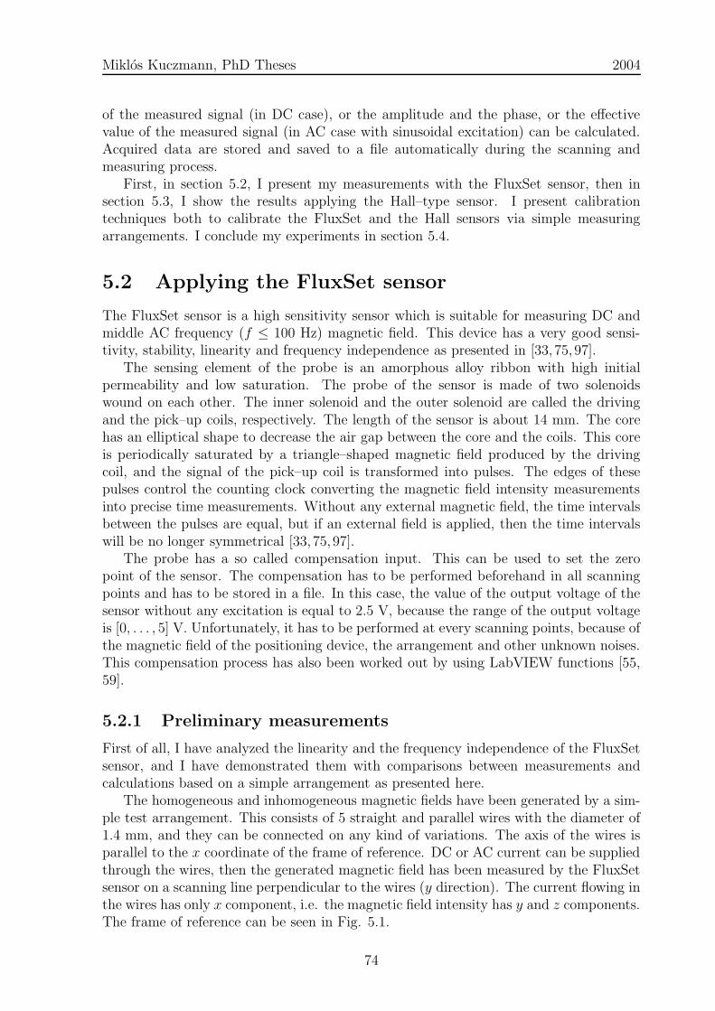
Miklos Kuczmann, PhD Theses 2004
of the measured signal (in DC case), or the amplitude and the phase, or the effectivevalue of the measured signal (in AC case with sinusoidal excitation) can be calculated.Acquired data are stored and saved to a file automatically during the scanning andmeasuring process.
First, in section 5.2, I present my measurements with the FluxSet sensor, then insection 5.3, I show the results applying the Hall–type sensor. I present calibrationtechniques both to calibrate the FluxSet and the Hall sensors via simple measuringarrangements. I conclude my experiments in section 5.4.
5.2 Applying the FluxSet sensor
The FluxSet sensor is a high sensitivity sensor which is suitable for measuring DC andmiddle AC frequency (f ≤ 100 Hz) magnetic field. This device has a very good sensi-tivity, stability, linearity and frequency independence as presented in [33, 75, 97].
The sensing element of the probe is an amorphous alloy ribbon with high initialpermeability and low saturation. The probe of the sensor is made of two solenoidswound on each other. The inner solenoid and the outer solenoid are called the drivingand the pick–up coils, respectively. The length of the sensor is about 14 mm. The corehas an elliptical shape to decrease the air gap between the core and the coils. This coreis periodically saturated by a triangle–shaped magnetic field produced by the drivingcoil, and the signal of the pick–up coil is transformed into pulses. The edges of thesepulses control the counting clock converting the magnetic field intensity measurementsinto precise time measurements. Without any external magnetic field, the time intervalsbetween the pulses are equal, but if an external field is applied, then the time intervalswill be no longer symmetrical [33, 75, 97].
The probe has a so called compensation input. This can be used to set the zeropoint of the sensor. The compensation has to be performed beforehand in all scanningpoints and has to be stored in a file. In this case, the value of the output voltage of thesensor without any excitation is equal to 2.5 V, because the range of the output voltageis [0, . . . , 5] V. Unfortunately, it has to be performed at every scanning points, because ofthe magnetic field of the positioning device, the arrangement and other unknown noises.This compensation process has also been worked out by using LabVIEW functions [55,59].
5.2.1 Preliminary measurements
First of all, I have analyzed the linearity and the frequency independence of the FluxSetsensor, and I have demonstrated them with comparisons between measurements andcalculations based on a simple arrangement as presented here.
The homogeneous and inhomogeneous magnetic fields have been generated by a sim-ple test arrangement. This consists of 5 straight and parallel wires with the diameter of1.4 mm, and they can be connected on any kind of variations. The axis of the wires isparallel to the x coordinate of the frame of reference. DC or AC current can be suppliedthrough the wires, then the generated magnetic field has been measured by the FluxSetsensor on a scanning line perpendicular to the wires (y direction). The current flowing inthe wires has only x component, i.e. the magnetic field intensity has y and z components.The frame of reference can be seen in Fig. 5.1.
74
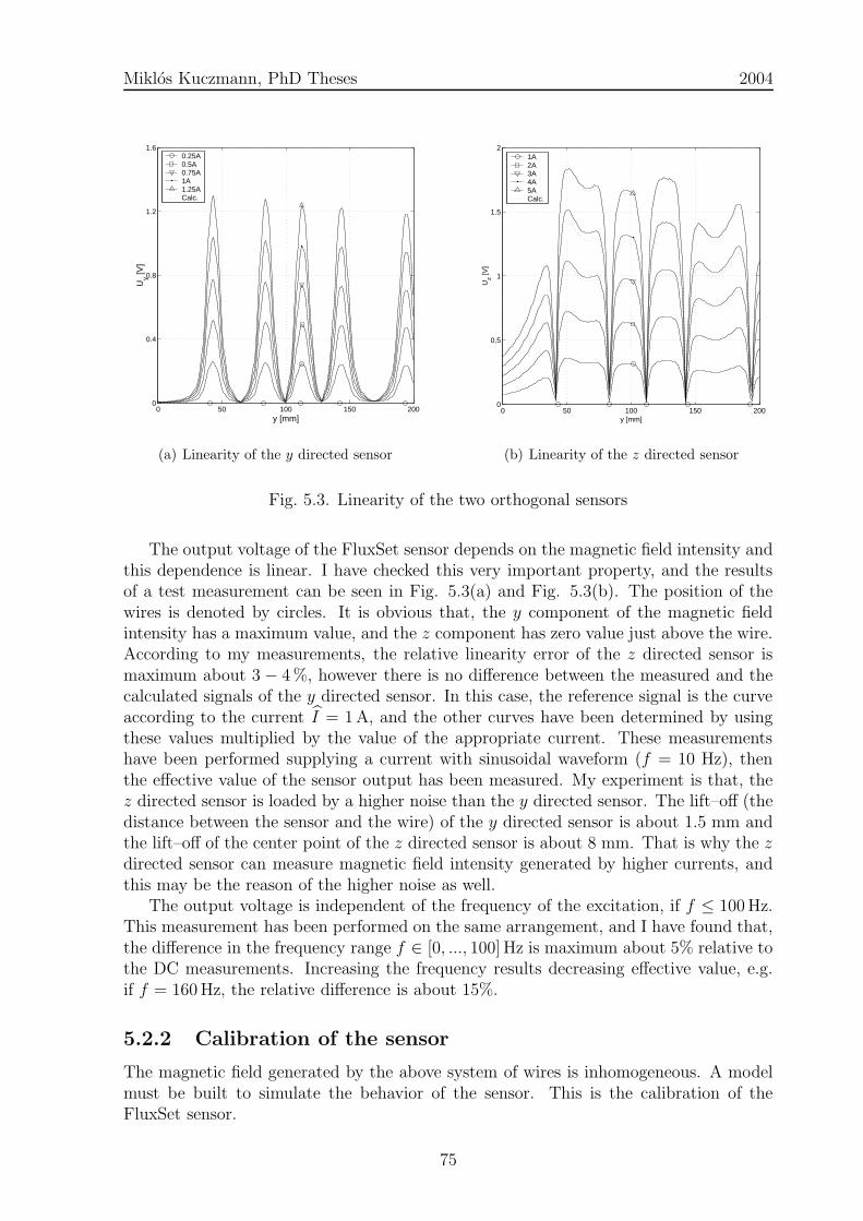
Miklos Kuczmann, PhD Theses 2004
0 50 100 150 2000
0.4
0.8
1.2
1.6
y [mm]
Uy [V
]
0.25A0.5A0.75A1A1.25ACalc.
(a) Linearity of the y directed sensor
0 50 100 150 2000
0.5
1
1.5
2
y [mm]
Uz [V
]
1A2A3A4A5ACalc.
(b) Linearity of the z directed sensor
Fig. 5.3. Linearity of the two orthogonal sensors
The output voltage of the FluxSet sensor depends on the magnetic field intensity andthis dependence is linear. I have checked this very important property, and the resultsof a test measurement can be seen in Fig. 5.3(a) and Fig. 5.3(b). The position of thewires is denoted by circles. It is obvious that, the y component of the magnetic fieldintensity has a maximum value, and the z component has zero value just above the wire.According to my measurements, the relative linearity error of the z directed sensor ismaximum about 3− 4 %, however there is no difference between the measured and thecalculated signals of the y directed sensor. In this case, the reference signal is the curveaccording to the current I = 1 A, and the other curves have been determined by usingthese values multiplied by the value of the appropriate current. These measurementshave been performed supplying a current with sinusoidal waveform (f = 10 Hz), thenthe effective value of the sensor output has been measured. My experiment is that, thez directed sensor is loaded by a higher noise than the y directed sensor. The lift–off (thedistance between the sensor and the wire) of the y directed sensor is about 1.5 mm andthe lift–off of the center point of the z directed sensor is about 8 mm. That is why the zdirected sensor can measure magnetic field intensity generated by higher currents, andthis may be the reason of the higher noise as well.
The output voltage is independent of the frequency of the excitation, if f ≤ 100 Hz.This measurement has been performed on the same arrangement, and I have found that,the difference in the frequency range f ∈ [0, ..., 100] Hz is maximum about 5% relative tothe DC measurements. Increasing the frequency results decreasing effective value, e.g.if f = 160 Hz, the relative difference is about 15%.
5.2.2 Calibration of the sensor
The magnetic field generated by the above system of wires is inhomogeneous. A modelmust be built to simulate the behavior of the sensor. This is the calibration of theFluxSet sensor.
75
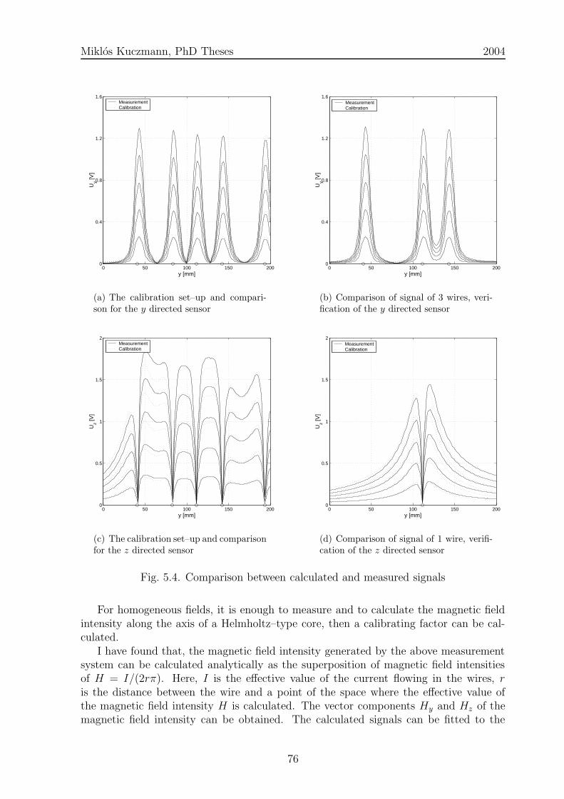
Miklos Kuczmann, PhD Theses 2004
0 50 100 150 2000
0.4
0.8
1.2
1.6
y [mm]
Uy [V
]
MeasurementCalibration
(a) The calibration set–up and compari-son for the y directed sensor
0 50 100 150 2000
0.4
0.8
1.2
1.6
y [mm]
Uy [V
]
MeasurementCalibration
(b) Comparison of signal of 3 wires, veri-fication of the y directed sensor
0 50 100 150 2000
0.5
1
1.5
2
y [mm]
Uz [V
]
MeasurementCalibration
(c) The calibration set–up and comparisonfor the z directed sensor
0 50 100 150 2000
0.5
1
1.5
2
y [mm]
Uz [V
]
MeasurementCalibration
(d) Comparison of signal of 1 wire, verifi-cation of the z directed sensor
Fig. 5.4. Comparison between calculated and measured signals
For homogeneous fields, it is enough to measure and to calculate the magnetic fieldintensity along the axis of a Helmholtz–type core, then a calibrating factor can be cal-culated.
I have found that, the magnetic field intensity generated by the above measurementsystem can be calculated analytically as the superposition of magnetic field intensitiesof H = I/(2rπ). Here, I is the effective value of the current flowing in the wires, ris the distance between the wire and a point of the space where the effective value ofthe magnetic field intensity H is calculated. The vector components Hy and Hz of themagnetic field intensity can be obtained. The calculated signals can be fitted to the
76
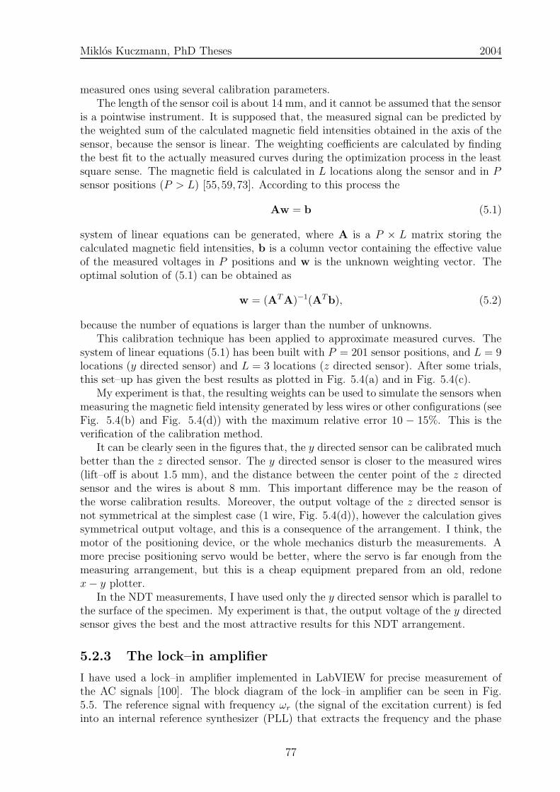
Miklos Kuczmann, PhD Theses 2004
measured ones using several calibration parameters.The length of the sensor coil is about 14 mm, and it cannot be assumed that the sensor
is a pointwise instrument. It is supposed that, the measured signal can be predicted bythe weighted sum of the calculated magnetic field intensities obtained in the axis of thesensor, because the sensor is linear. The weighting coefficients are calculated by findingthe best fit to the actually measured curves during the optimization process in the leastsquare sense. The magnetic field is calculated in L locations along the sensor and in Psensor positions (P > L) [55, 59, 73]. According to this process the
Aw = b (5.1)
system of linear equations can be generated, where A is a P × L matrix storing thecalculated magnetic field intensities, b is a column vector containing the effective valueof the measured voltages in P positions and w is the unknown weighting vector. Theoptimal solution of (5.1) can be obtained as
w = (ATA)−1(ATb), (5.2)
because the number of equations is larger than the number of unknowns.This calibration technique has been applied to approximate measured curves. The
system of linear equations (5.1) has been built with P = 201 sensor positions, and L = 9locations (y directed sensor) and L = 3 locations (z directed sensor). After some trials,this set–up has given the best results as plotted in Fig. 5.4(a) and in Fig. 5.4(c).
My experiment is that, the resulting weights can be used to simulate the sensors whenmeasuring the magnetic field intensity generated by less wires or other configurations (seeFig. 5.4(b) and Fig. 5.4(d)) with the maximum relative error 10 − 15%. This is theverification of the calibration method.
It can be clearly seen in the figures that, the y directed sensor can be calibrated muchbetter than the z directed sensor. The y directed sensor is closer to the measured wires(lift–off is about 1.5 mm), and the distance between the center point of the z directedsensor and the wires is about 8 mm. This important difference may be the reason ofthe worse calibration results. Moreover, the output voltage of the z directed sensor isnot symmetrical at the simplest case (1 wire, Fig. 5.4(d)), however the calculation givessymmetrical output voltage, and this is a consequence of the arrangement. I think, themotor of the positioning device, or the whole mechanics disturb the measurements. Amore precise positioning servo would be better, where the servo is far enough from themeasuring arrangement, but this is a cheap equipment prepared from an old, redonex− y plotter.
In the NDT measurements, I have used only the y directed sensor which is parallel tothe surface of the specimen. My experiment is that, the output voltage of the y directedsensor gives the best and the most attractive results for this NDT arrangement.
5.2.3 The lock–in amplifier
I have used a lock–in amplifier implemented in LabVIEW for precise measurement ofthe AC signals [100]. The block diagram of the lock–in amplifier can be seen in Fig.5.5. The reference signal with frequency ωr (the signal of the excitation current) is fedinto an internal reference synthesizer (PLL) that extracts the frequency and the phase
77
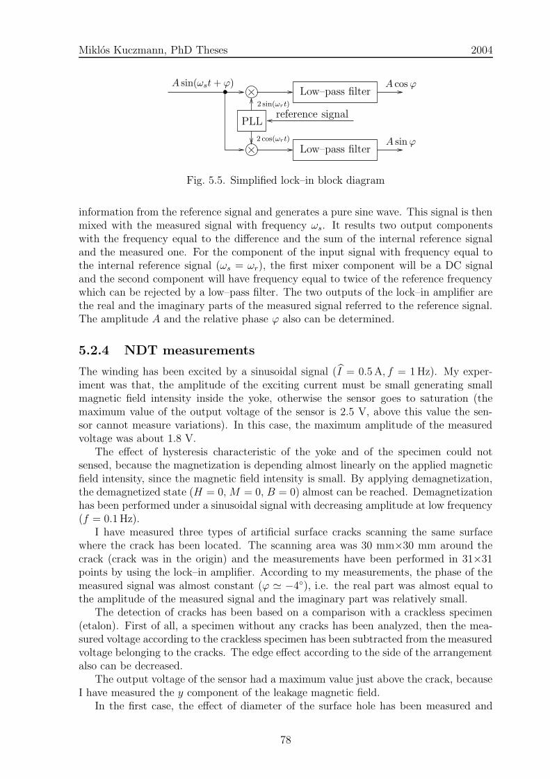
Miklos Kuczmann, PhD Theses 2004PSfrag replacements
A sin(ωst + ϕ)
reference signal2 sin(ωrt)
2 cos(ωrt)
PLL
A cos ϕ
A sin ϕLow–pass filter
Low–pass filter
Fig. 5.5. Simplified lock–in block diagram
information from the reference signal and generates a pure sine wave. This signal is thenmixed with the measured signal with frequency ωs. It results two output componentswith the frequency equal to the difference and the sum of the internal reference signaland the measured one. For the component of the input signal with frequency equal tothe internal reference signal (ωs = ωr), the first mixer component will be a DC signaland the second component will have frequency equal to twice of the reference frequencywhich can be rejected by a low–pass filter. The two outputs of the lock–in amplifier arethe real and the imaginary parts of the measured signal referred to the reference signal.The amplitude A and the relative phase ϕ also can be determined.
5.2.4 NDT measurements
The winding has been excited by a sinusoidal signal (I = 0.5 A, f = 1 Hz). My exper-iment was that, the amplitude of the exciting current must be small generating smallmagnetic field intensity inside the yoke, otherwise the sensor goes to saturation (themaximum value of the output voltage of the sensor is 2.5 V, above this value the sen-sor cannot measure variations). In this case, the maximum amplitude of the measuredvoltage was about 1.8 V.
The effect of hysteresis characteristic of the yoke and of the specimen could notsensed, because the magnetization is depending almost linearly on the applied magneticfield intensity, since the magnetic field intensity is small. By applying demagnetization,the demagnetized state (H = 0, M = 0, B = 0) almost can be reached. Demagnetizationhas been performed under a sinusoidal signal with decreasing amplitude at low frequency(f = 0.1 Hz).
I have measured three types of artificial surface cracks scanning the same surfacewhere the crack has been located. The scanning area was 30 mm×30 mm around thecrack (crack was in the origin) and the measurements have been performed in 31×31points by using the lock–in amplifier. According to my measurements, the phase of themeasured signal was almost constant (ϕ ' −4), i.e. the real part was almost equal tothe amplitude of the measured signal and the imaginary part was relatively small.
The detection of cracks has been based on a comparison with a crackless specimen(etalon). First of all, a specimen without any cracks has been analyzed, then the mea-sured voltage according to the crackless specimen has been subtracted from the measuredvoltage belonging to the cracks. The edge effect according to the side of the arrangementalso can be decreased.
The output voltage of the sensor had a maximum value just above the crack, becauseI have measured the y component of the leakage magnetic field.
In the first case, the effect of diameter of the surface hole has been measured and
78
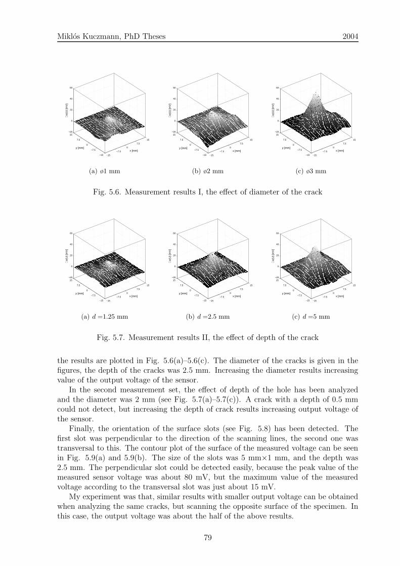
Miklos Kuczmann, PhD Theses 2004
−15
−7.5
0
7.5
15
−15
−7.5
0
7.5
15−20
0
20
40
60
x [mm]y [mm]
ℜe(
U)
[mV
]
(a) ø1 mm
−15
−7.5
0
7.5
15
−15
−7.5
0
7.5
15−20
0
20
40
60
x [mm]y [mm]
ℜe(
U)
[mV
](b) ø2 mm
−15
−7.5
0
7.5
15
−15
−7.5
0
7.5
15−20
0
20
40
60
x [mm]y [mm]
ℜe(
U)
[mV
]
(c) ø3 mm
Fig. 5.6. Measurement results I, the effect of diameter of the crack
−15
−7.5
0
7.5
15
−15
−7.5
0
7.5
15−20
0
20
40
60
x [mm]y [mm]
ℜe(
U)
[mV
]
(a) d =1.25 mm
−15
−7.5
0
7.5
15
−15
−7.5
0
7.5
15−20
0
20
40
60
x [mm]y [mm]
ℜe(
U)
[mV
]
(b) d =2.5 mm
−15
−7.5
0
7.5
15
−15
−7.5
0
7.5
15−20
0
20
40
60
x [mm]y [mm]
ℜe(
U)
[mV
]
(c) d =5 mm
Fig. 5.7. Measurement results II, the effect of depth of the crack
the results are plotted in Fig. 5.6(a)–5.6(c). The diameter of the cracks is given in thefigures, the depth of the cracks was 2.5 mm. Increasing the diameter results increasingvalue of the output voltage of the sensor.
In the second measurement set, the effect of depth of the hole has been analyzedand the diameter was 2 mm (see Fig. 5.7(a)–5.7(c)). A crack with a depth of 0.5 mmcould not detect, but increasing the depth of crack results increasing output voltage ofthe sensor.
Finally, the orientation of the surface slots (see Fig. 5.8) has been detected. Thefirst slot was perpendicular to the direction of the scanning lines, the second one wastransversal to this. The contour plot of the surface of the measured voltage can be seenin Fig. 5.9(a) and 5.9(b). The size of the slots was 5 mm×1 mm, and the depth was2.5 mm. The perpendicular slot could be detected easily, because the peak value of themeasured sensor voltage was about 80 mV, but the maximum value of the measuredvoltage according to the transversal slot was just about 15 mV.
My experiment was that, similar results with smaller output voltage can be obtainedwhen analyzing the same cracks, but scanning the opposite surface of the specimen. Inthis case, the output voltage was about the half of the above results.
79

Miklos Kuczmann, PhD Theses 2004
PSfrag replacements
x
y
perpendicular transversalscan
nin
glin
es
Fig. 5.8. The manufactured perpendicular and transversal slots
−15 −7.5 0 7.5 15−15
−7.5
0
7.5
15
x [mm]
y [m
m]
(a) The perpendicular slot
−15 −7.5 0 7.5 15−15
−7.5
0
7.5
15
x [mm]
y [m
m]
(b) The transversal slot
Fig. 5.9. Top view of the measured voltage
A 2D adaptive noise–removal filtering has been performed on measured signals bythe Wiener filter implemented in the Image Processing Toolbox of MATLAB [99]. Thislowpass filters the intensity image that has been degraded by additive noise and Wienerfiltering causes a little smoothing as well.
80

Miklos Kuczmann, PhD Theses 2004
−200 −100 0 100 2000
0.5
1
1.5
2
z [mm]
UH
all [V
]
0.5 A
1 A
2 A
3 A
4 A
(a) The linearity and calibration results
−200 −100 0 100 2000.4
0.55
0.7
0.85
1
z [mm]
UH
all [V
]
1Hz5Hz10Hz20Hz
(b) The frequency independence
Fig. 5.10. Examination of the Hall–type sensor
5.3 Applying the Hall–type sensor
A 3D Hall–type sensor has been developed in the frame of a student work under mysupervisorship [42]. The sensor is a GaAs sensor, and the type is OH10003. The pre-pared probe contains three orthogonal Hall sensors as close to each others as possible.The output signal of the Hall sensor is very small (in this case, it is in the range of10 . . . 100µV), so it is amplified by an operational amplifier (to the range of 1 . . . 10 V).This is a simpler and cheaper instrument than the FluxSet sensor. The size of the ap-plied Hall sensor is 2.9 mm × 1.5 mm× 1.1 mm, and it is much smaller than the lengthof the coil in the FluxSet sensor (14 mm).
Classically, the Hall effect in a semiconducting medium is based on the Lorentz forceF = Q(v × B) when a particle with charge Q is moving with velocity v within amagnetic field B. If a long, flat current–carrying conductor is placed in a magnetic field,the moving charges will experience a force perpendicular to the direction of the currentand of the magnetic field. It results an un–even charge distribution and gives rise to anelectric field E which generates a measurable Hall–voltage which is proportional to themagnetic flux density [69, 70].
5.3.1 Preliminary measurements and calibration
However the sensor has satisfactory linearity with respect to the magnetic field intensityand small temperature coefficient according to the catalogue of the sensor, we haveanalyzed the linearity and the frequency independence of the sensor and its electronics.
Test measurements have been performed by a calibrating coil which length wasl = 340 mm, the radius was about r = 50 mm and the number of turns was N = 305.The Hall sensor has been placed into the axis of the coil and the output voltage has beenmeasured in the range of z ∈ [−155, . . . , 155] mm, if z = 0 is the center point of the coil.The magnetic field intensity along the axis of the coil can be calculated easily by the
81
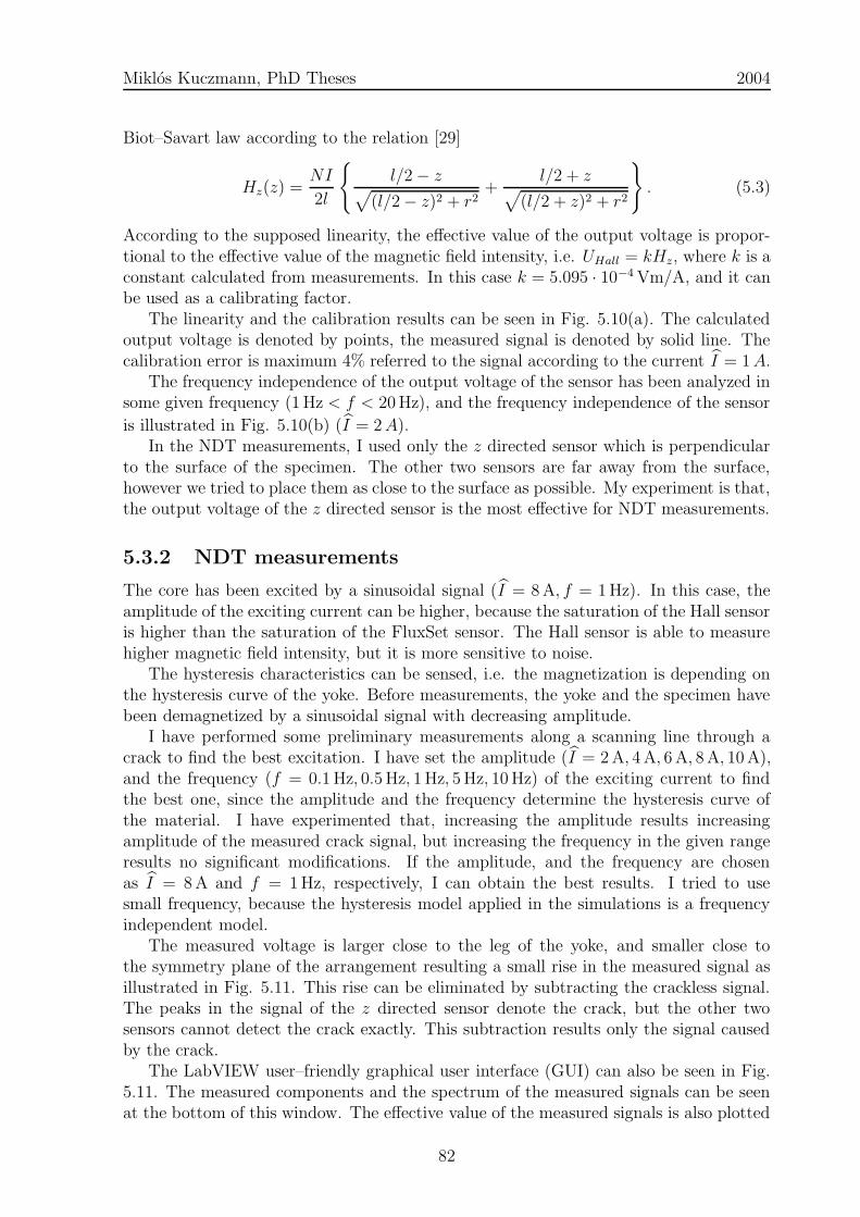
Miklos Kuczmann, PhD Theses 2004
Biot–Savart law according to the relation [29]
Hz(z) =NI
2l
l/2− z√
(l/2− z)2 + r2+
l/2 + z√(l/2 + z)2 + r2
. (5.3)
According to the supposed linearity, the effective value of the output voltage is propor-tional to the effective value of the magnetic field intensity, i.e. UHall = kHz, where k is aconstant calculated from measurements. In this case k = 5.095 · 10−4 Vm/A, and it canbe used as a calibrating factor.
The linearity and the calibration results can be seen in Fig. 5.10(a). The calculatedoutput voltage is denoted by points, the measured signal is denoted by solid line. Thecalibration error is maximum 4% referred to the signal according to the current I = 1A.
The frequency independence of the output voltage of the sensor has been analyzed insome given frequency (1 Hz < f < 20 Hz), and the frequency independence of the sensor
is illustrated in Fig. 5.10(b) (I = 2A).In the NDT measurements, I used only the z directed sensor which is perpendicular
to the surface of the specimen. The other two sensors are far away from the surface,however we tried to place them as close to the surface as possible. My experiment is that,the output voltage of the z directed sensor is the most effective for NDT measurements.
5.3.2 NDT measurements
The core has been excited by a sinusoidal signal (I = 8 A, f = 1 Hz). In this case, theamplitude of the exciting current can be higher, because the saturation of the Hall sensoris higher than the saturation of the FluxSet sensor. The Hall sensor is able to measurehigher magnetic field intensity, but it is more sensitive to noise.
The hysteresis characteristics can be sensed, i.e. the magnetization is depending onthe hysteresis curve of the yoke. Before measurements, the yoke and the specimen havebeen demagnetized by a sinusoidal signal with decreasing amplitude.
I have performed some preliminary measurements along a scanning line through acrack to find the best excitation. I have set the amplitude (I = 2 A, 4 A, 6 A, 8 A, 10 A),and the frequency (f = 0.1 Hz, 0.5 Hz, 1 Hz, 5 Hz, 10 Hz) of the exciting current to findthe best one, since the amplitude and the frequency determine the hysteresis curve ofthe material. I have experimented that, increasing the amplitude results increasingamplitude of the measured crack signal, but increasing the frequency in the given rangeresults no significant modifications. If the amplitude, and the frequency are chosenas I = 8 A and f = 1 Hz, respectively, I can obtain the best results. I tried to usesmall frequency, because the hysteresis model applied in the simulations is a frequencyindependent model.
The measured voltage is larger close to the leg of the yoke, and smaller close tothe symmetry plane of the arrangement resulting a small rise in the measured signal asillustrated in Fig. 5.11. This rise can be eliminated by subtracting the crackless signal.The peaks in the signal of the z directed sensor denote the crack, but the other twosensors cannot detect the crack exactly. This subtraction results only the signal causedby the crack.
The LabVIEW user–friendly graphical user interface (GUI) can also be seen in Fig.5.11. The measured components and the spectrum of the measured signals can be seenat the bottom of this window. The effective value of the measured signals is also plotted
82

Miklos Kuczmann, PhD Theses 2004
and saved in a file. Important data can be set through the GUI: the coordinates ofthe scanning area, the number of steps above the specimen, the number of samples perperiods and the number of periods to be measured.
The bridge, where the sensor is moving in the y direction is made of aluminum, butunfortunately, the mechanics of it disturbs the measured signal. I have prepared a spacerwhich enables to move the sensor far away from this mechanics. A comparison betweenthe two measurements can be seen in Fig. 5.12, where the 1st measurement is performedwithout the spacer and the 2nd is with using the spacer. This figure shows the outputvoltage of the z directed sensor. Measurements are closer to the calculated results whenthe effect of mechanics has been eliminated. I have realized this problem after developingthe FEM software and I have made the measurements again.
I have measured the same artificial surface cracks as analyzed by the FluxSet sensor.In this case, the scanning area was 40 mm×40 mm around the crack and the measure-ments are performed 41×41 points (the crack is in the origin). After measuring 5 periods,the effective value of the measured voltage has been calculated, then the crackless signalhas been subtracted from it.
The output voltage of the sensor had zero value just above the crack and had maxi-mum and minimum values before and after the crack, because I have measured applyingthe z directed sensor. These two peaks results much accurate contour plots than the onepeak of the y component.
In the first case, the effect of diameter of the surface hole has been measured and theresults are plotted in Fig. 5.13(a)–5.13(c). The diameter of the cracks is given in thefigures, the depth of the cracks was 2.5 mm. Increasing the diameter results increasingvalue of the output voltage.
In the second measurement set, the effect of depth of the hole has been analyzed,when the diameter was 2 mm (see Fig. 5.14(a)–5.14(c)). A crack with a depth of 0.5 mmcould be detected again, but increasing the depth of the crack results in increasing outputvoltage.
Finally, the orientation of the same surface slots has been detected (see Fig. 5.8).The first slot was perpendicular to the direction of the scanning line, the second one wastransversal to this. The top view of the measured voltages can be seen in Fig. 5.15(a) andFig. 5.15(b). The perpendicular slot could be detected easily, because the peak valueof the measured voltage was about 0.15 V, and the maximum value of the measuredvoltage according to the transversal slot was just about 0.06 V, but the contour plot ofthe measurements show the orientation of the crack. The orientation and the size of theslots is deducible. Measuring the z component gives more accurate contour plots thanmeasuring the y component.
5.4 Conclusions of the measurements
I have experimented that, the FluxSet sensor is more sensitive than the Hall–type sensor,i.e. the FluxSet sensor can measure small magnetic fields. The Hall sensor is able tomeasure much higher magnetic fields.
The Hall sensor has a very small size, but I think, a matrix with 3×3, or 5×5 sensorswould give better and more accurate measurements. Of course, more sensitive type ofsensor should be used. There exists a problem of the demagnetizing process: the powersupply can generate a current with the maximum peak value of 20 A. It seems that, it is
83
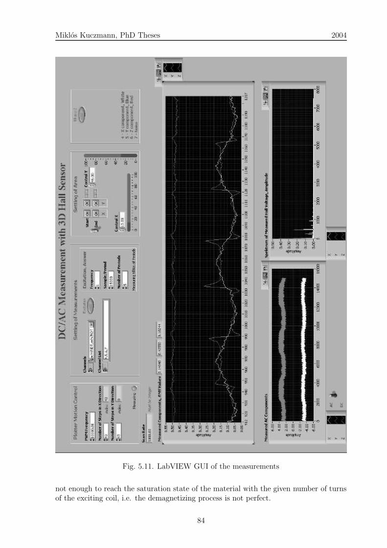
Miklos Kuczmann, PhD Theses 2004
Fig. 5.11. LabVIEW GUI of the measurements
not enough to reach the saturation state of the material with the given number of turnsof the exciting coil, i.e. the demagnetizing process is not perfect.
84
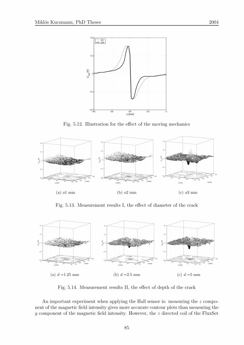
Miklos Kuczmann, PhD Theses 2004
−40 −30 −20 −10 0−0.2
−0.1
0
0.1
0.2
y [mm]
UH
all [V
]
1st2nd
Fig. 5.12. Illustration for the effect of the moving mechanics
170180
190200
210
−40−30
−20−10
0−0.2
−0.1
0
0.1
0.2
x [mm]y [mm]
UH
all [V
]
(a) ø1 mm
170180
190200
210
−40−30
−20−10
0−0.2
−0.1
0
0.1
0.2
x [mm]y [mm]
UH
all [V
]
(b) ø2 mm
170180
190200
210
−40−30
−20−10
0−0.2
−0.1
0
0.1
0.2
x [mm]y [mm]
UH
all [V
]
(c) ø3 mm
Fig. 5.13. Measurement results I, the effect of diameter of the crack
170180
190200
210
−40−30
−20−10
0−0.2
−0.1
0
0.1
0.2
x [mm]y [mm]
UH
all [V
]
(a) d =1.25 mm
170180
190200
210
−40−30
−20−10
0−0.2
−0.1
0
0.1
0.2
x [mm]y [mm]
UH
all [V
]
(b) d =2.5 mm
170180
190200
210
−40−30
−20−10
0−0.2
−0.1
0
0.1
0.2
x [mm]y [mm]
UH
all [V
]
(c) d =5 mm
Fig. 5.14. Measurement results II, the effect of depth of the crack
An important experiment when applying the Hall sensor is: measuring the z compo-nent of the magnetic field intensity gives more accurate contour plots than measuring they component of the magnetic field intensity. However, the z directed coil of the FluxSet
85

Miklos Kuczmann, PhD Theses 2004
(a) The perpendicular slot
170 180 190 200 210−40
−30
−20
−10
0
x [mm]
y [m
m]
(b) The transversal slot
Fig. 5.15. Top view of the measured voltage
sensor is far from the surface of the specimen.I have developed a 3D nonlinear FEM software to simulate the presented measure-
ment system to compare calculations and the above measurements. I only focus on themeasurements performed by the Hall sensor. Other important measured signals withcomparisons with the simulated ones are also shown in the next section.
5.5 Simulation of the installed NDT equipment
The same mathematical formulations can be used as described in the previous chapter,but applying the 3D shape functions in tetrahedral finite elements (I = 4 and K = 6)and the 3D NN based vector hysteresis model [61].
On the basis of the 2D problem presented in the previous chapter, I have developedthe 3D numerical simulation of the built NDT equipment. A global to local model hasbeen used: first, a global model has been applied to determine the potential distributionnear the crack, then a local domain including the crack has been investigated. Theglobal model has been applied to determine the artificial boundary conditions of thelocal model.
Comparisons between the measured and the simulated crack signals are presented atthe end of this section.
5.5.1 Global–local model in 3D calculations
The generated meshes, the boundary conditions and properties of the calcu-
lations
The size of a manufactured crack is very small comparing with the size of the wholearrangement: e.g. the diameter of a surface hole is maximum 2.5 mm and its depth ismaximum 5 mm, the size of the U–shaped yoke is 320×240×5 mm, i.e. the order is
86
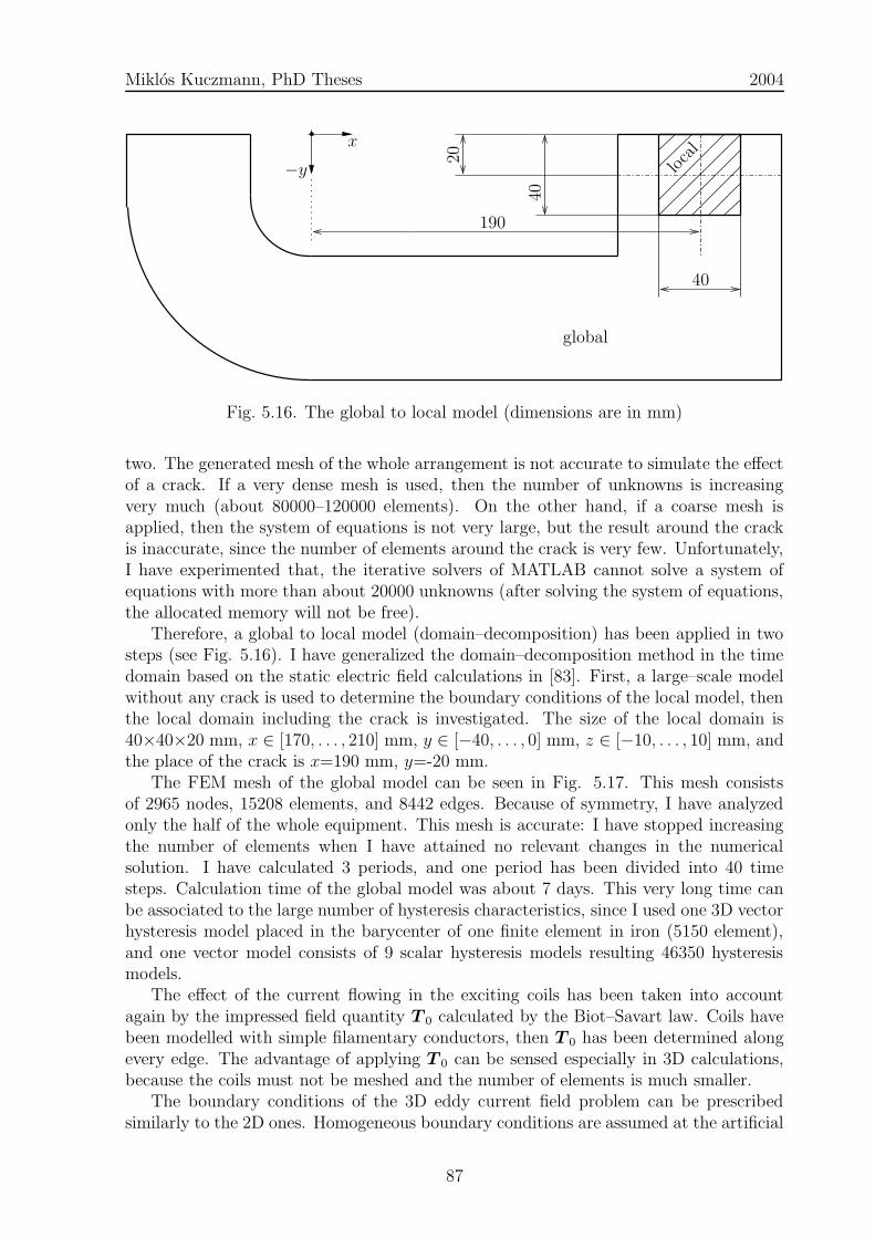
Miklos Kuczmann, PhD Theses 2004
PSfrag replacements 190
20
x
−y
40
40
global
local
Fig. 5.16. The global to local model (dimensions are in mm)
two. The generated mesh of the whole arrangement is not accurate to simulate the effectof a crack. If a very dense mesh is used, then the number of unknowns is increasingvery much (about 80000–120000 elements). On the other hand, if a coarse mesh isapplied, then the system of equations is not very large, but the result around the crackis inaccurate, since the number of elements around the crack is very few. Unfortunately,I have experimented that, the iterative solvers of MATLAB cannot solve a system ofequations with more than about 20000 unknowns (after solving the system of equations,the allocated memory will not be free).
Therefore, a global to local model (domain–decomposition) has been applied in twosteps (see Fig. 5.16). I have generalized the domain–decomposition method in the timedomain based on the static electric field calculations in [83]. First, a large–scale modelwithout any crack is used to determine the boundary conditions of the local model, thenthe local domain including the crack is investigated. The size of the local domain is40×40×20 mm, x ∈ [170, . . . , 210] mm, y ∈ [−40, . . . , 0] mm, z ∈ [−10, . . . , 10] mm, andthe place of the crack is x=190 mm, y=-20 mm.
The FEM mesh of the global model can be seen in Fig. 5.17. This mesh consistsof 2965 nodes, 15208 elements, and 8442 edges. Because of symmetry, I have analyzedonly the half of the whole equipment. This mesh is accurate: I have stopped increasingthe number of elements when I have attained no relevant changes in the numericalsolution. I have calculated 3 periods, and one period has been divided into 40 timesteps. Calculation time of the global model was about 7 days. This very long time canbe associated to the large number of hysteresis characteristics, since I used one 3D vectorhysteresis model placed in the barycenter of one finite element in iron (5150 element),and one vector model consists of 9 scalar hysteresis models resulting 46350 hysteresismodels.
The effect of the current flowing in the exciting coils has been taken into accountagain by the impressed field quantity T 0 calculated by the Biot–Savart law. Coils havebeen modelled with simple filamentary conductors, then T 0 has been determined alongevery edge. The advantage of applying T 0 can be sensed especially in 3D calculations,because the coils must not be meshed and the number of elements is much smaller.
The boundary conditions of the 3D eddy current field problem can be prescribedsimilarly to the 2D ones. Homogeneous boundary conditions are assumed at the artificial
87
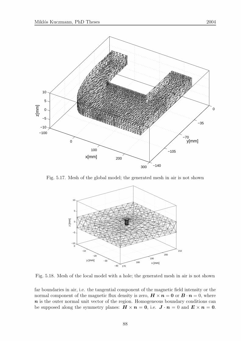
Miklos Kuczmann, PhD Theses 2004
−100
0
100
200
300 −140
−105
−70
−35
0
−10
−5
0
5
10
y[mm]
x[mm]
z[m
m]
Fig. 5.17. Mesh of the global model; the generated mesh in air is not shown
170
180
190
200
210
−40
−30
−20
−10
0−10
−5
0
5
10
x [mm]y [mm]
z [m
m]
Fig. 5.18. Mesh of the local model with a hole; the generated mesh in air is not shown
far boundaries in air, i.e. the tangential component of the magnetic field intensity or thenormal component of the magnetic flux density is zero, H ×n = 0 or B ·n = 0, wheren is the outer normal unit vector of the region. Homogeneous boundary conditions canbe supposed along the symmetry planes: H × n = 0, i.e. J · n = 0 and E × n = 0.
88
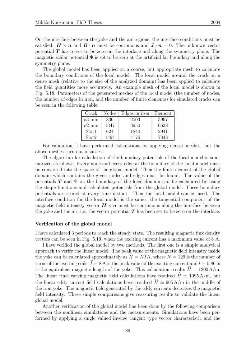
Miklos Kuczmann, PhD Theses 2004
On the interface between the yoke and the air regions, the interface conditions must besatisfied: H × n and B · n must be continuous and J · n = 0. The unknown vectorpotential T has to set to be zero on the interface and along the symmetry plane. Themagnetic scalar potential Ψ is set to be zero at the artificial far boundary and along thesymmetry plane.
The global model has been applied on a coarse, but appropriate mesh to calculatethe boundary conditions of the local model. The local model around the crack on adense mesh (relative to the size of the analyzed domain) has been applied to calculatethe field quantities more accurately. An example mesh of the local model is shown inFig. 5.18. Parameters of the generated meshes of the local model (the number of nodes,the number of edges in iron, and the number of finite elements) for simulated cracks canbe seen in the following table:
Crack Nodes Edges in iron Elementø3 mm 830 2503 3997ø2 mm 1347 3950 6638Slot1 624 1840 2941Slot2 1494 4176 7343
For validation, I have performed calculations by applying denser meshes, but theabove meshes turn out a success.
The algorithm for calculation of the boundary potentials of the local model is sum-marized as follows. Every node and every edge at the boundary of the local model mustbe converted into the space of the global model. Then the finite element of the globaldomain which contains the given nodes and edges must be found. The value of thepotentials T and Ψ on the boundary of the local domain can be calculated by usingthe shape functions and calculated potentials from the global model. These boundarypotentials are stored at every time instant. Then the local model can be used. Theinterface condition for the local model is the same: the tangential component of themagnetic field intensity vector H × n must be continuous along the interface betweenthe yoke and the air, i.e. the vector potential T has been set to be zero on the interface.
Verification of the global model
I have calculated 3 periods to reach the steady state. The resulting magnetic flux densityvectors can be seen in Fig. 5.19, when the exciting current has a maximum value of 8 A.
I have verified the global model by two methods. The first one is a simple analyticalapproach to verify the linear model. The peak value of the magnetic field intensity insidethe yoke can be calculated approximately as H = NI/l, where N = 129 is the number of
turns of the exciting coils, I = 8 A is the peak value of the exciting current and l = 0.86 mis the equivalent magnetic length of the yoke. This calculation results H = 1200 A/m.
The linear time varying magnetic field calculations have resulted H ' 1095 A/m, but
the linear eddy current field calculations have resulted H ' 905 A/m in the middle ofthe iron yoke. The magnetic field generated by the eddy currents decreases the magneticfield intensity. These simple comparisons give reassuring results to validate the linearglobal model.
Another verification of the global model has been done by the following comparisonbetween the nonlinear simulations and the measurements. Simulations have been per-formed by applying a single valued inverse tangent type vector characteristic and the
89

Miklos Kuczmann, PhD Theses 2004
−105 −15 75 165 255−140
−100
−60
−20
20
x [mm]
y [m
m]
Fig. 5.19. The resulting magnetic flux density vectors inside the yoke simulated by theglobal model(there are two layers, where the vectors are drawn: z = −1.25 mm and z = 1.25 mm)
3D NN based isotropic vector hysteresis model identified by the presented method (seeChapter 3). I have used real measurements applying a toroidal shape coil made of thesame material as the specimen and as the yoke. I have supposed that, the material is anisotropic magnetic material. Characteristics are shown Fig. 5.20(a). The measurementwas the following: I have measured the induced voltage of a coil wound the yoke’s leg andI have calculated it as well. The number of turns of the measurement coil was N = 100.The Fig. 5.20(b) shows this comparison. These comparisons show the very good agree-ment between the simulations and the measurements, especially when I have applied theNN based vector hysteresis characteristic. However, applying the simpler inverse tangenttype characteristic has also resulted accurate solution. The induced voltage simulatedby the inverse tangent type characteristic is higher than the induced voltage simulatedby the NN based vector hysteresis model, because the inverse tangent type characteristicis steeper and the induced voltage depends on the shape of the characteristic, i.e.
Ui = −Nd
dt
∫
S
B · n dS,
where S is the area of the yoke’s leg. These simulations show the applicability of theNN based vector hysteresis model and of the proposed identification technique. Thecorrectness of the applied global FEM mesh, the boundary conditions, the iteration
90

Miklos Kuczmann, PhD Theses 2004
−2500 −1250 0 1250 2500−1.6
−0.8
0
0.8
1.6
H [A/m]
B [T
]
(a) The applied single valued and hystere-sis characteristics
0 0.25 0.5 0.75 1−0.6
−0.3
0
0.3
0.6
t [s]
Ui [V
]
HysteresisArcus tangentMeasurement
(b) Measured and calculated inducedvoltages
Fig. 5.20. Verification of the global model
scheme have also been validated by these calculations and comparisons.
Surface integrals in the local model
When the global model is applied, the boundary conditions on the artificial far boundaryand on the symmetry plane can be subscribed easily. In the case of the local model, thesurface integrals on the boundary cannot be neglected, because the local model is notsymmetrical. If the local model is used, then the boundary conditions can be calculatedfrom the global model as described above, and the terms from the surface integrals mustbe included into the assembled system of linear equations.
The following surface integrals are derived only in the 3D eddy current field problemusing the local model.
There is a time varying magnetic field problem in the air region Ωn, therefore theequation (4.10) has to be used, but the boundary integral term on Γn cannot be neglected,i.e. ∮
Γn
Nj
µ0T 0 − µ0∇Ψ
· ndΓ 6= 0. (5.4)
This surface integral must be calculated at every triangular face of a tetrahedron con-necting to the boundary as
6∑
k=1
µ0
∫
S
Nj(W k ·n) dS T0,k −4∑
i=1
µ0
∫
S
Nj(∇Ni) · n dSΨi, (5.5)
where S is the area of the face of the tetrahedron connecting to the boundary of thelocal model and n is the outer normal unit vector of this surface triangle. The first sumis known and it has to be subtracted from the right hand side of (4.13). There are threenodes connecting to the boundary which potential value Ψi are known from the globalmodel. These surface integral terms must also be assembled to the right hand side of
91

Miklos Kuczmann, PhD Theses 2004
(4.13). There is only one node with unknown potential and the according term must beassembled to the left hand side of (4.13).
There is an eddy current field problem inside the specimen Ωc, that is the boundaryintegral term from the integral (4.28) must be applied, i.e.
∮
Γc
Nj
µT 0 + µT − µ∇Ψ
· n dΓ 6= 0. (5.6)
This surface integral must be calculated at every triangular face of a tetrahedron con-necting to the boundary as
6∑
k=1
µ
∫
S
Nj(W k · n) dS T0,k +6∑
k=1
µ
∫
S
Nj(W k · n) dS Tk
−4∑
i=1
µ
∫
S
Nj(∇Ni) · ndS Ψi.
(5.7)
The surface integral in (4.24)∮
Γc
W j × 1
σ∇× T 0 +
1
σ∇× T
· n dΓ (5.8)
gives
6∑
k=1
1
σ
∫
S
W j · (∇×W k × n) dST0,k
+
6∑
k=1
1
σ
∫
S
W j · (∇×W k × n) dSTk.
(5.9)
There are three nodes and three edges of a tetrahedron connecting to the boundary ofthe local model. The according potentials Ψi and Tk are known from the global modeland these surface integral terms must be assembled to the right hand side of (4.29)and (4.27). There is only one node and three edges with unknown potentials and theaccording terms must be assembled to the left hand side of (4.29) and (4.27).
In the case of taking into account the hysteresis characteristic of the nonlinear media,the surface integral ∮
Γc
Nj(RFP · n) dΓ (5.10)
from the weak form of the partial differential equation (4.36) must also be inserted. Thevalue of RFP ·n is constant in one finite element and must be subtracted from the righthand side of the according equations. In this case, the above surface integrals should bemodified as µ = µFP .
A comparison between the magnetic induction vectors inside the specimen accordingto the area of the local domain, calculated using the global model and using the localmodel can be seen in Fig. 5.21(a) and Fig. 5.21(b). The maximum relative difference be-tween the calculated induction vectors is about 5%. This comparison shows the accuracyof the global–local model.
The global model is a time consuming model, but this must be used only once. Thelocal model can be applied to simulate all of the measured cracks (the computation timeof the local model is about 2 hours).
92

Miklos Kuczmann, PhD Theses 2004
160 175 190 205 220−60
−45
−30
−15
0
x [mm]
y [m
m]
(a) Using the global model
160 175 190 205 220−60
−45
−30
−15
0
x [mm]
y [m
m]
(b) Using the local model
Fig. 5.21. Comparison between the resulting B vectors (there are two layers, where the normalizedvectors are drawn: z = −1.25 mm and z = 1.25 mm)
5.5.2 Simulation of the Hall sensor
Calculation of the output signal
The gradient of the measured and of the calculated signal ∂U∂y
is increasing near to thecrack, because this signal is varying rapidly. Let us have a look at to Fig. 5.22. Thesimulated signal is narrower than the measured one, therefore I have used the followingcalibration process (it may be that, the mechanics of the positioning device has disturbedthe measurements, however I have used a spacer as presented in the section 5.3.2).
First of all, I have calculated the magnetic field intensity vector H = T 0 − ∇Ψat the scanning points along the scanning line through the center of the crack abovethe specimen (x = 190 mm, y = −40, . . . , 0 mm). I have supposed that, the sensor is apointwise instrument, i.e. I have just multiplied the z–component of the magnetic fieldintensity vector (Hz) by the calibrating factor k = 5.095 · 10−4 Vm/A which has beendetermined by the calibrating solenoid (see section 5.3.1). This results a very narrowsignal as can be seen in Fig. 5.22, however the simulated peak values are very closeto the measured ones. This signal is a bit staged, because ∇Ψ is constant in a finiteelement, since I have used first order shape functions.
Second, I have supposed that, the sensor is not a pointwise instrument, but a verysmall one with the length of 2.9 mm. I have calculated the magnetic field intensity at5 given points along the axis of the sensor and a linear combination of these magneticfield intensities multiplied by the calibration factor k results in a better simulation (itis denoted by k′H). This is a similar calibration process presented in the calibration ofthe FluxSet sensor (see section 5.2.2). The above calibration technique has to be used,because the length of the Hall sensor is commensurable with the size of the cracks.
93
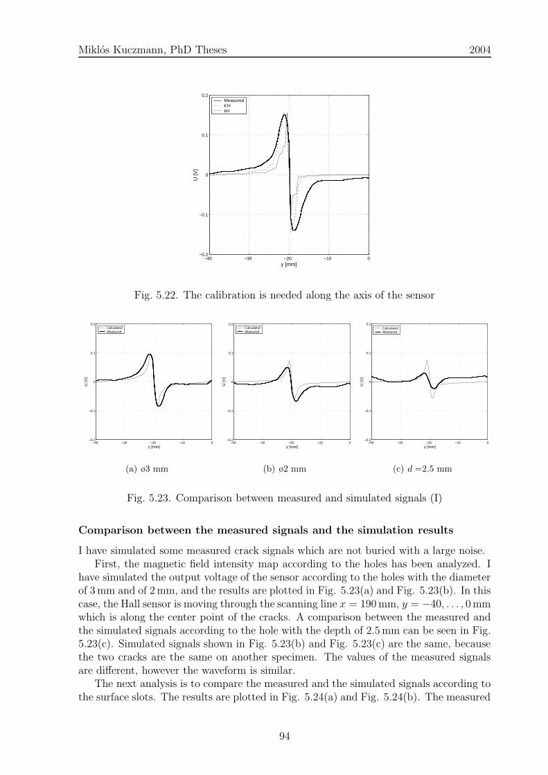
Miklos Kuczmann, PhD Theses 2004
−40 −30 −20 −10 0−0.2
−0.1
0
0.1
0.2
y [mm]
U [V
]
Measuredk’HkH
Fig. 5.22. The calibration is needed along the axis of the sensor
−40 −30 −20 −10 0−0.2
−0.1
0
0.1
0.2
y [mm]
U [V
]
CalculatedMeasured
(a) ø3 mm
−40 −30 −20 −10 0−0.2
−0.1
0
0.1
0.2
y [mm]
U [V
]
CalculatedMeasured
(b) ø2 mm
−40 −30 −20 −10 0−0.2
−0.1
0
0.1
0.2
y [mm]
U [V
]
CalculatedMeasured
(c) d =2.5 mm
Fig. 5.23. Comparison between measured and simulated signals (I)
Comparison between the measured signals and the simulation results
I have simulated some measured crack signals which are not buried with a large noise.First, the magnetic field intensity map according to the holes has been analyzed. I
have simulated the output voltage of the sensor according to the holes with the diameterof 3 mm and of 2 mm, and the results are plotted in Fig. 5.23(a) and Fig. 5.23(b). In thiscase, the Hall sensor is moving through the scanning line x = 190 mm, y = −40, . . . , 0 mmwhich is along the center point of the cracks. A comparison between the measured andthe simulated signals according to the hole with the depth of 2.5 mm can be seen in Fig.5.23(c). Simulated signals shown in Fig. 5.23(b) and Fig. 5.23(c) are the same, becausethe two cracks are the same on another specimen. The values of the measured signalsare different, however the waveform is similar.
The next analysis is to compare the measured and the simulated signals according tothe surface slots. The results are plotted in Fig. 5.24(a) and Fig. 5.24(b). The measured
94
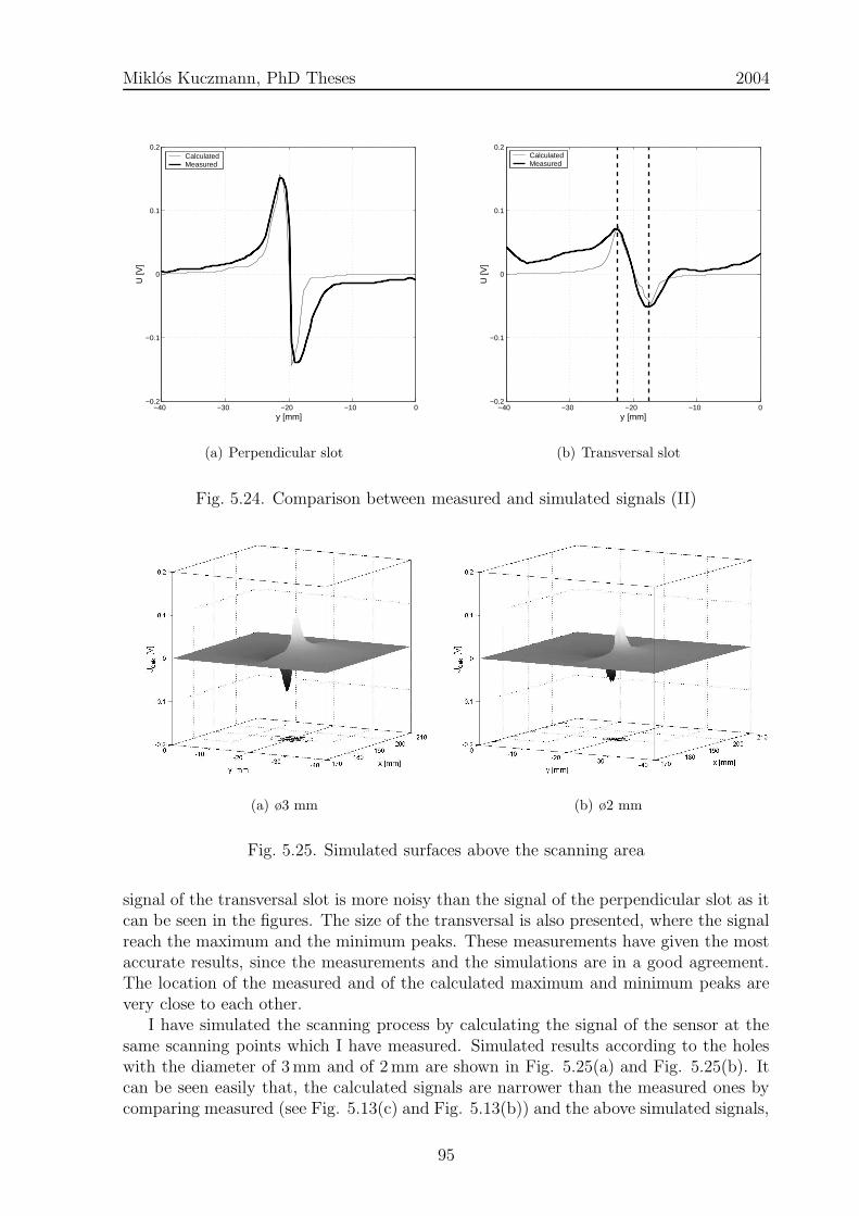
Miklos Kuczmann, PhD Theses 2004
−40 −30 −20 −10 0−0.2
−0.1
0
0.1
0.2
y [mm]
U [V
]
CalculatedMeasured
(a) Perpendicular slot
−40 −30 −20 −10 0−0.2
−0.1
0
0.1
0.2
y [mm]
U [V
]
CalculatedMeasured
(b) Transversal slot
Fig. 5.24. Comparison between measured and simulated signals (II)
(a) ø3 mm (b) ø2 mm
Fig. 5.25. Simulated surfaces above the scanning area
signal of the transversal slot is more noisy than the signal of the perpendicular slot as itcan be seen in the figures. The size of the transversal is also presented, where the signalreach the maximum and the minimum peaks. These measurements have given the mostaccurate results, since the measurements and the simulations are in a good agreement.The location of the measured and of the calculated maximum and minimum peaks arevery close to each other.
I have simulated the scanning process by calculating the signal of the sensor at thesame scanning points which I have measured. Simulated results according to the holeswith the diameter of 3 mm and of 2 mm are shown in Fig. 5.25(a) and Fig. 5.25(b). Itcan be seen easily that, the calculated signals are narrower than the measured ones bycomparing measured (see Fig. 5.13(c) and Fig. 5.13(b)) and the above simulated signals,
95
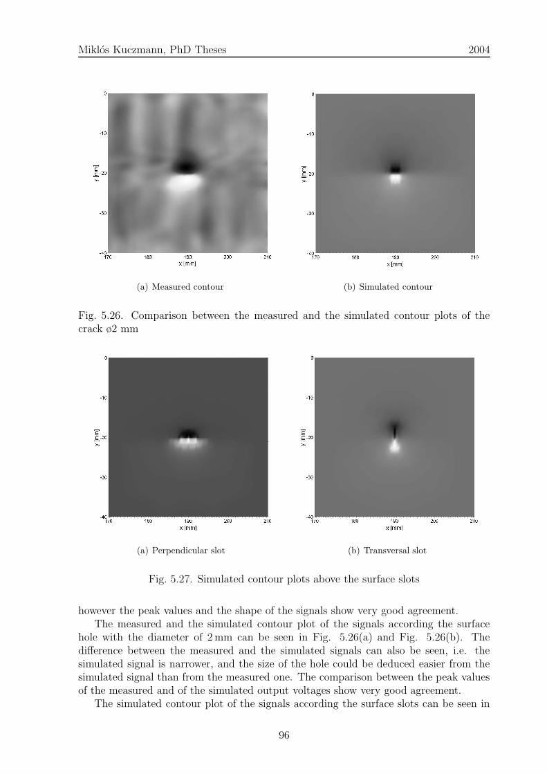
Miklos Kuczmann, PhD Theses 2004
(a) Measured contour (b) Simulated contour
Fig. 5.26. Comparison between the measured and the simulated contour plots of thecrack ø2 mm
(a) Perpendicular slot (b) Transversal slot
Fig. 5.27. Simulated contour plots above the surface slots
however the peak values and the shape of the signals show very good agreement.The measured and the simulated contour plot of the signals according the surface
hole with the diameter of 2 mm can be seen in Fig. 5.26(a) and Fig. 5.26(b). Thedifference between the measured and the simulated signals can also be seen, i.e. thesimulated signal is narrower, and the size of the hole could be deduced easier from thesimulated signal than from the measured one. The comparison between the peak valuesof the measured and of the simulated output voltages show very good agreement.
The simulated contour plot of the signals according the surface slots can be seen in
96
Miklos Kuczmann, PhD Theses 2004
Fig. 5.27(a) and Fig. 5.27(b). The size and the orientation of the slots can be determinedeasier from simulations than from measurements (see Fig. 5.15(a) and Fig. 5.15(b)). Itcan also be seen that, the simulated signals are narrower than the measured ones.
The location and the orientation of the manufactured surface holes and slots can bedetermined easier from simulations than from measurements, since simulated signals arenarrower than the measured ones and calculations are not buried with noise.
Conclusions
A more precise measurement arrangement would result much better agreement betweenthe measurements and the simulations, however I could reach my aim, i.e. to simulateaccurately the test equipment, to check the developed nonlinear FEM software and theNN based vector hysteresis characteristic by the comparisons between the measurementsand the simulations.
The comparison between the measured and the simulated induced voltages has shownvery good agreement. This global quantity can be measured easily, because the errorsfrom measurements are averaging. The crack signals are measured in the scanning pointsand this measurement is buried with local noise and local measurement error.
5.6 New scientific results
3. Thesis I have confirmed the three dimensional nonlinear simulation technique bycomparing simulated and measured results. I have worked out a measurement systemwhich is able to detect the surface cracks of a specimen and I have developed the nu-merical simulation of this arrangement. I have worked out the global to local model(domain–decomposition) of the arrangement in the time domain. The boundary condi-tions of the local model have been calculated by using the global model. I have comparedthe simulated and the measured output signal of the Hall sensor, and these comparisonsshow very good agreement.
3.a I have built a measurement system to analyze the FluxSet sensor and the Hall–type sensor in the field of measuring the crack signals. I have examined the signalscorresponding to cracks with different size and shape. I have worked out calibrationmethods to predict the output voltage of the sensors by using simple arrangements.The measurements are performed by using the software environment LabVIEW.
3.b I have developed the three dimensional nonlinear numerical analysis of the builtnondestructive testing measurement system and I have used the finite elementmethod and the T ,Ψ−Ψ potential formulation. I have developed a global to localmodel of the built arrangement in the time domain. I have used the global modelwithout any crack to predict the artificial boundary conditions of the local modelwhere the crack has been taken into account. I have developed the surface integralsobtained from the weak form of the partial differential equations necessary to usein the local model. I have implemented the identified three dimensional neuralnetwork based isotropic vector hysteresis model to the eddy current field problem byapplying the fixed–point iteration technique and the B–scheme of the polarizationmethod. The comparisons between the measured crack signals performed by theHall sensor and the simulation results show the good applicability of the developedmodel.
97
Chapter 6
Summary of the new scientific
results
Finally, I gather my research work in the field of hysteresis modeling and of the FEM.
1. Thesis I have developed a new scalar hysteresis operator based on the function ap-proximation capability of the neural networks to simulate the behavior of ferromagneticmaterials. I have represented the first order reversal curves with a surface by introduc-ing the variable ξ and I have approximated this surface by neural network technique.I have built a knowledge–base which contains if–then type rules about the behavior ofthe hysteresis characteristics. I have shown the applicability of the model by comparingsimulated and measured results. I have taken into account the vectorial behavior of themagnetic field intensity and the magnetic flux density by applying the neural networkbased vector hysteresis model, and I have recommended a new identification procedureto build up the vector model. I have worked out the three dimensional anisotropic vectorhysteresis model, and I have analyzed the behavior of the developed vector models.
1.a I have developed a new neural network based mathematical representation of thescalar hysteresis operator. I have handled the multivalued property of the hysteresischaracteristics by introducing the new variable ξ associated with the measured firstorder reversal curves. This preprocessing can be applied on any kind of hysteresischaracteristics. I have built a knowledge–base which contains if–then type rulesabout the behavior of the hysteresis characteristics. This is the memory mechanismof the model. I have realized the identification procedure by the training of theneural networks. I have built a measurement system to measure hysteresis curveson a toroidal shape C19 structural steel, and I have used these measurementsto show the applicability of the neural network based scalar hysteresis model bycomparing measurements and simulation results.
1.b I have developed the two dimensional and the three dimensional isotropic vectorhysteresis models based on the neural network based scalar model. I have workedout an original and new identification procedure based on the measurable Everettfunction both to predict two dimensional and three dimensional isotropic hysteresischaracteristics. I have compared the measured and the predicted curves and I haveshown the behavior of the vector model in linear and in rotational magnetic fields.
98
Miklos Kuczmann, PhD Theses 2004
1.c I have developed the two dimensional and the three dimensional neural networkbased anisotropic vector hysteresis models by the means of Fourier expansion ofthe measured Everett function of the anisotropic material. I have generalized thetwo dimensional model in three dimensions as a theoretical expansion of the twodimensional model, and I have recommended an identification procedure to fit tomeasured curves. I have compared the measured and the predicted curves and Ihave shown the behavior of the vector model in linear and in rotational magneticfields, finally I have compared the isotropic and the anisotropic models.
2. Thesis I have implemented the developed neural network based vector hysteresismodel to the finite element method. I have applied the Ψ and the T ,Ψ − Ψ potentialformulations, because these directly give the magnetic field intensity vector which isthe input variable of the direct vector hysteresis model. I have used the nodal and theedge shape functions for the approximation of the potentials. I have handled the neuralnetwork based vector hysteresis model by applying the B–scheme of the polarizationmethod, and I have solved the linearized system of equations by the fixed–point iterationtechnique. I have used an under–relaxation scheme to speed up the convergence of themethod. This results in a convergent and a well applicable method to solve both timevarying magnetic field problem and eddy current field problem.
3. Thesis I have confirmed the three dimensional nonlinear simulation technique bycomparing simulated and measured results. I have worked out a measurement systemwhich is able to detect the surface cracks of a specimen and I have developed the nu-merical simulation of this arrangement. I have worked out the global to local model(domain–decomposition) of the arrangement in the time domain. The boundary condi-tions of the local model have been calculated by using the global model. I have comparedthe simulated and the measured output signal of the Hall sensor, and these comparisonsshow very good agreement.
3.a I have built a measurement system to analyze the FluxSet sensor and the Hall–type sensor in the field of measuring the crack signals. I have examined the signalscorresponding to cracks with different size and shape. I have worked out calibrationmethods to predict the output voltage of the sensors by using simple arrangements.The measurements are performed by using the software environment LabVIEW.
3.b I have developed the three dimensional nonlinear numerical analysis of the builtnondestructive testing measurement system and I have used the finite elementmethod and the T ,Ψ−Ψ potential formulation. I have developed a global to localmodel of the built arrangement in the time domain. I have used the global modelwithout any crack to predict the artificial boundary conditions of the local modelwhere the crack has been taken into account. I have developed the surface integralsobtained from the weak form of the partial differential equations necessary to usein the local model. I have implemented the identified three dimensional neuralnetwork based isotropic vector hysteresis model to the eddy current field problem byapplying the fixed–point iteration technique and the B–scheme of the polarizationmethod. The comparisons between the measured crack signals performed by theHall sensor and the simulation results show the good applicability of the developedmodel.
99

Chapter 7
Conclusions and future
developments
A neural network based hysteresis operator has been presented in this work. The iden-tification of the scalar model is a simple training method on measured and preprocessedfirst order reversal curves. The vector hysteresis model in 2D and in 3D has also beenimplemented for both the isotropic and the anisotropic case. While the scalar hysteresismeasurement is an easy task, the measurement of the 2D vector hysteresis character-istics is a great challenge, and it is a large project. There are some problems on themeasurements of the magnetic field intensity as can be found in the literature. It is afuture work to build a vector hysteresis measurement system in our laboratory. The 3Dvector hysteresis measurement is an open question, I have not found any paper aboutthis topic. I have developed a theoretical representation of the 3D anisotropic model,but I think there may be several generalizations of this model.
I have built a measurement system which is able to perform simple NDT measure-ments. It is important to note that, I have used this system to check my computations.Building a measurement system is a hard work, because several problems can be emerged,such as the system noise, and other phenomena, that disturb the measurement. This istrue for all measurement systems. I have found that, a more precise x–y positioning de-vice should be used. The positioning device may be the weak point in my measurements.I think that, a more sensitive sensor can be built by using the developed Hall–type probeand by making a sensor matrix with 3×3 or 5×5 sensors.
At the last part of the presented work, I have presented the implemented FEM codeto simulate the built measurement system. As it was presented, the main goal was tobuild the developed neural network based vector hysteresis model into the FEM. Thenonlinear behavior of the hysteresis characteristics has been handled by the fixed–pointtechnique which results relatively long computation time, especially in 3D case using theglobal model. The Newton–Raphson type iterative methods may give faster solution.
Another and very important observation is that, a stand alone software should be usedto simulate any arrangement, when applying the FEM. The software package MATLABis very powerful, but this is very slow in this case, i.e. a C–code (especially a parallelcode running on a parallel computer) may be a better alternative. Higher order shapefunctions may also give better approximation as well [101, 102]. In the case of higherorder shape functions, some case study have to be done (e.g. solving TEAM problems).
100

Bibliography
[1] A.A. Adly and S.K. Abd-El-Hafiz. Using neural networks in the identification ofPreisach-type hysteresis models. IEEE Trans. on Magn., 34(3):629–635, 1998.
[2] A.A. Adly, S.K. Abd-El-Hafiz, and I.D. Mayergoyz. Identification of vectorPreisach models from arbitrary measured data using neural networks. MagneticImaging and Modeling, 87(9):6821–6823, 2000.
[3] R. Albanese, E. Coccorese, G. De Santis, R. Martone, and C. Create. A neuralnetwork based technique for non destructive evaluation exploiting soft computingconcepts. Nondestructive Testing of Materials, pages 1–12, 1995.
[4] M. Berend and E. Berend. Biological Lexicon for Students (in Hungarian).Akademia Kiado, Budapest, 1996.
[5] G. Bertotti. Hysteresis in Magnetism. Academic Press, 1998.
[6] O. Bıro. Edge element formulations of eddy current problems. Comput. Meth.Appl. Mech. Engrg., 169:391–405, 1999.
[7] O. Bıro, K. Hollaus, J. Pavo, and K. Preis. Numerical computation of the mag-netic field due to a crack in a conducting plate. Electromagnetic NondestructiveEvaluation (V), pages 11–15, 2001.
[8] I. Bojtar and Zs. Gaspar. Finite Element Method for Engineers. TERC, Budapest,2003.
[9] A. Bossavit. Computational Electromagnetism. Academic Press, Boston, 1998.
[10] I.D.O. Bottauscio, D. Chiarabaglio, C. Ragusa, M. Chiampi, and M. Repetto.Analysis of isotropic materials with vector hysteresis. IEEE Trans. on Magn.,34:1258–1260, 1997.
[11] O. Bottuascio, M. Chiampi, and C. Ragusa. Transient analysis of hysteretic fieldproblems using fixed point technique. IEEE Trans. on Magn., 39(3):1179–1182,2003.
[12] J. Bowler. Pulsed eddy current inversion for the determination of crack shape.Electromagnetic Nondestructive Evaluation, pages 263–269, 1997.
[13] T. Chady, M. Enokizono, R. Sikora, and K. Takeuchi. Eddy current testing of con-crete structures. International Journal of Applied Electromagnetics and Mechanics,15:33–37, 2001/2002.
i
Miklos Kuczmann, PhD Theses 2004
[14] T. Chady, M. Enokizono, and R. Sykora. Signal restroration using dynamic neuralnetwork model for eddy current nondestructive testing. IEEE Trans. on Magn.,37(5):3737–3740, 2001.
[15] T. Chady, M. Enokizono, T. Todaka, Y. Tsuchida, and R. Sykora. Evaluation of theJSAEM round robin test samples using multi-frequency excitation and spectogrammethod. Electromagnetic Nondestructive Evaluation (V), pages 171–178, 2001.
[16] W. Cheng, K. Miya, and K. Demachi. Application of FEM-BEM coupling methodto eddy current testing problem. Electromagnetic Nondestructive Evaluation (IV),pages 17–24, 2000.
[17] M. Chiampi, A.L. Negro, and M. Tartaglia. A finite element method to computethree-dimensional magnetic field distribution in transformer cores. IEEE Trans.on Magn., MAG-16(6):1413–1419, 1980.
[18] S. Chikazumi. Physics of Magnetism. John Wiley and Sons, New York, 1964.
[19] C. Christodoulou and M. Georgiopoulos. Applications of Neural Networks in Elec-tromagnetics. Artech House, Norwood, 2001.
[20] S. Cincotti. Approximation properties of a PWL circuit model of hysteresis. Phys-ica B, 275:216–222, 2000.
[21] V. Cingoski. Study on Improved Three-Dimensional Electromagnetic Field Compu-tations Utilizing Vector Edge Finite Elements. PhD thesis, Hiroshima University,1996.
[22] Kikusui Electronics Corporation. Operation Manual, PBX Series. KIKUSUI,Japan, 1992-2000.
[23] M. Dotterweich, G. Szymanski, and M. Waszak. Approximation of the Preisachfunction using feedforward neural network approximator. International Journal ofApplied Electromagnetics and Mechanics, 17 (1-3):243–250, 2003.
[24] L.R. Dupre, O. Bottuascio, M. Chiampi, M. Repetto, and J.A.A. Melkebeek. Mod-eling of electromagnetic phenomena in soft magnetic materials under unidirectionaltime periodic flux excitation. IEEE Trans. on Magn., 35(5):4171–4184, 1999.
[25] G. Horvath (editor). Neural Networks with Applications (in Hungarian).Muegyetemi Kiado, Budapest, 1998.
[26] G. Stoyan (editor). Matlab, version 4. and 5. (in Hungarian). TypoTex, Budapest,1999.
[27] V.R. Vemuri (editor). Artificial Neural Networks, Concepts and Control Applica-tions. IEEE Computer Soc. Press, Los Alamos, California, 1992.
[28] M. Enokizono, T. Chady, T. Todaka, and Y. Tsuchida. Frequency scanning in NDEusing multi-frequency excitation system. Energy and Information in Non-LinearSystems, pages 90–93, 2001.
ii

Miklos Kuczmann, PhD Theses 2004
[29] Gy. Fodor. Electromagnetic Fields (in Hungarian). Muegyetemi Kiado, 1996.
[30] J. Fuzi. Computationally efficient rate dependent hysteresis model. COMPEL,18(3):445–457, 1999.
[31] J. Fuzi, A. Ivanyi, and Zs. Szabo. Preisach model with continuous output inelectrical circuit analysis. Journal of Electrical Engineering, Bratislava, Slovakia,48:18–21, 1997.
[32] J. Fuzi, Gy. Szekely, and Zs. Szabo. Experimental construction of classical Preisachmodel. Proceedings of the 8th IGTE Symposium, Graz, Austria, pages 452–457,1998.
[33] A. Gasparics, Cs.S. Daroczi, S. Calcagno, V. Mollo, R. Albanese, and J. Pavo.Comparative study on the performance of ECT probes. Electromagnetic Nonde-structive Evaluation (IV), pages 227–234, 2000.
[34] V. Gorican, A. Hamler, M. Jesenik, B. Stumberger, and M. Trlep. Unreliable deter-mination of vector B in 2-D SST. Journal of Magnetism and Magnetic Materials,254-255:130–132, 2003.
[35] Sz. Gyimothy. Adaptıv automatikus halogeneralas a vegeselem modszerhez. PhDthesis, Budapest University of Technology and Economics, 2003.
[36] M. Hano, T. Miyamura, and M. Hotta. Finite element eddy current analysis bynovel mixed-order vector elements. International Journal of Applied Electromag-netics and Mechanics, 14:19–22, 2001/2002.
[37] H. Hoshikawa, K. Koyama, H. Hayakawa, and H. Morisaki. Study on the appro-priate exciter-to-detector distance in remote field eddy current tubing inspection.Electromagnetic Nondestructive Evaluation (IV), pages 71–78, 2000.
[38] National Instruments. LabVIEW, Basics Manual. -, 2000.
[39] A. Ivanyi. Hysteresis Models in Electromagnetic Computation. Akademia Kiado,Budapest, 1997.
[40] A. Ivanyi. Magnetic Field Computation with R-functions. Akademia Kiado, Bu-dapest, 1998.
[41] A. Ivanyi. Continuous and Discrete Simulations in Electrodinamics (in Hungar-ian). Akademia Kiado, Budapest, 2003.
[42] Sz. Jagasics. Building a 3D Hall-type sensor. Budapest, 2003.
[43] D.C. Jiles. Introduction to Magnetism and Magnetic Material. Chapman and Hall,London, 1991.
[44] Gy. Kadar and E.D. Torre. Hysteresis modeling: I. Noncongruency. IEEE Trans.on Magn., MAG-23(5):2820–2822, 1987.
[45] Gy. Kadar and E.D. Torre. Determination of the bilinear product Preisach function.J.Appl. Phys., 63(8):3001–3003, 1988.
iii
Miklos Kuczmann, PhD Theses 2004
[46] Gy. Kajdi. Material Testing with Eddy Currents (in Hungarian). ProfessionalExtention and Company, Budapest, 1990.
[47] P. Kis and A. Ivanyi. Computer aided magnetic hysteresis measurement in Lab-VIEW environment. Journal of Electrical Engineering, 53(10):173–176, 2002.
[48] P. Kis, M. Kuczmann, and A. Ivanyi. Hysteresis measurement in LabVIEW. Phys-ica B, 343:357–363, 2004.
[49] P.I. Koltermann, J.P.A. Bastos, N. Sadowski, N.J. Batistela, A. Kost, L. Janicke,and K. Miethner. Nonlinear magnetic field model by FEM taking into accounthysteresis characteristics with M-B variables. IEEE Trans. on Magn., 38(2):897–900, 2002.
[50] M. Kuczmann and A. Ivanyi. Neural network based scalar hysteresis model. In-ternational Journal of Applied Electromagnetics and Mechanics, pages 225–230,2001/2002.
[51] M. Kuczmann and A. Ivanyi. Isotropic and anisotropic vector hysteresis modelbased on neural networks. Journal of Electrical Engineering 9/s, pages 73–76,2002.
[52] M. Kuczmann and A. Ivanyi. Measuring and identification of scalar hys-teresis characteristics applying neural network based hysteresis (in Hungarian).Hıradastechnika, LVII:4–9, 2002.
[53] M. Kuczmann and A. Ivanyi. Neural network model of magnetic hysteresis. COM-PEL, pages 367–376, 2002.
[54] M. Kuczmann and A. Ivanyi. A new neural-network-based scalar hysteresis model.IEEE Trans. on Magn., pages 857–860, 2002.
[55] M. Kuczmann and A. Ivanyi. Calibration and measurement with 3D FluxSet sensor(in Hungarian). Hıradastechnika, pages 34–37, 2003.
[56] M. Kuczmann and A. Ivanyi. Neural network model for scalar and vector hysteresis.Journal of Electrical Engineering 1-2, pages 12–21, 2003.
[57] M. Kuczmann and A. Ivanyi. Vector hysteresis model based on neural network.COMPEL, pages 730–743, 2003.
[58] M. Kuczmann and A. Ivanyi. Nonlinear 2D edge element based FEM in T , ψ − ψformulation. Proceedings of the 9th OPTIM Conference, Brasov, Romania, pages41–48, 2004.
[59] M. Kuczmann and A. Ivanyi. Calibration of FluxSet sensor. Proceedings of the12th International Symposium on Theoretical and Electrical Engineering, Warsaw,Poland, pages 389–392, July 16-19, 2003.
[60] M. Kuczmann and A. Ivanyi. Neural network based scalar hysteresis model. Pro-ceedings of the 10th International Symposium on Applied Electromagnetics andMechanics, Tokyo, Japan, pages 493–494, May 13-16, 2001.
iv

Miklos Kuczmann, PhD Theses 2004
[61] M. Kuczmann and A. Ivanyi. Simulation of a nondestructive testing measurementsystem. Proceedings of the 11th IGTE Symposium, Seggau Castle, Austria, pages376–381, September 13-15, 2004.
[62] M. Kuczmann and A. Ivanyi. Vector hysteresis model based on neural network.Proceedings of the 10th International IGTE Symposium, Graz, Austria, pages 453–458, September 16-18, 2002.
[63] M. Kuczmann and A. Ivanyi. Neural network based simulation of scalar hystere-sis. Proceedings of the 10th International Symposium on Electromagnetic Fields inElectrical Engineering, Cracow, Poland, pages 413–416, September 20-22, 2001.
[64] M. Kuczmann, P. Kis, A. Ivanyi, and J. Fuzi. Vector hysteresis measurement.Physica B, 343:390–394, 2004.
[65] D. Lederer, H. Igarashi, A. Kost, and T. Honma. Effective reluctivity calculationversus time step calculation of magnetic shielding with ferromagnetic material.COMPEL, 18:410–421, 1999.
[66] Y. Liu, A. Bondeson, R. Bergstrom, M.G. Larson, and K. Samuelsson. Methods forcomputing eddy currents in laminated materials using edge elements. Proceedingsof the 10th IGTE Symposium, Graz, Austria, pages 351–356, 2002.
[67] I.D. Mayergoyz. Mathematical Models of Hysteresis. Springer-Verlag, New York,1991.
[68] O. Mihalache, G. Preda, T. Uchimoto, K. Demachi, and K. Miya. Crack recon-struction in ferromagetic materials using nonlinear FEM-BEM scheme and neuralnetworks. Electromagnetic Nondestructive Evaluation (V), pages 67–74, 2001.
[69] D. Minkov, T. Shoji, and J. Lee. Determining the depth distribution of mag-netic dipoles in the dipole model of surface crack. Electromagnetic NondestructiveEvaluation (IV), pages 9–16, 2000.
[70] D. Minkov, T. Shoji, and J. Lee. Crack inversion based on measuring leakagemagnetic field by InAs Hall element. Electromagnetic Nondestructive Evaluation(V), pages 113–120, 2001.
[71] M. Oka and M. Enokizono. High sensitive ECT probe using a differential typemagneto-impedance effect sensor for a small reverse-side crack. ElectromagneticNondestructive Evaluation (IV), pages 95–102, 2000.
[72] C. Papusoi and A. Stancu. Anhysteretic remanent susceptibility and the movingPreisach model. IEEE Trans. on Magn., 29(1):77–81, 1993.
[73] J. Pavo, O. Bıro, and K. Hollaus. Calculation of the field map from the measure-ment data of the FluxSet sensor. COMPEL, 20(2):404–416, 1998.
[74] G. Preda, O. Mihalache, B. Cranganu-Cretu, Z. Chen, and K. Miya. FEM-BEMcoupling and neural network for reconstruction of crack shape from simulated pulseeddy current signals. Energy and Information in Non-Linear Systems, pages 110–113, 2001.
v
Miklos Kuczmann, PhD Theses 2004
[75] K. Preis, I. Bardi, O. Bıro, K.R. Richter, J. Pavo, A. Gasparics, and I. Ticar.Numerical simulation and design of a FluxSet sensor by finite element method.IEEE Trans. on Magn., 34(5):3475–3478, 1998.
[76] J. Prohaszka. Material Science (in Hungarian). Tankoknyvkiado, Budapest, 1993.
[77] C. Ragusa and M. Repetto. Anisotropic vector Preisach model and magnetic fieldsolutions. COMPEL, 18(3):458–468, 1999.
[78] C. Ragusa and M. Repetto. Accurate analysis of magnetic devices with anisotropicvector hysteresis. Physica B, 275:92–98, 2000.
[79] M. Saghafifar, A. Kundu, and A. Nafalski. Dynamic magnetic hysteresis modellingusing Elman recurrent neural network. International Journal of Applied Electro-magnetics and Mechanics, 13:209–214, 2001/2002.
[80] A. Salvini and P. Del Vecchio. Neural network and Fourier descriptor macro-modeling dynamic hysteresis. Proceedings of the 12th COMPUMAG Conference,Sapporo, Japan, pages 228–229, October 25-28, 1999.
[81] E.S. Sazonov. An Automated Damage Detection System for Armoured VehicleLaunched Bridge. PhD thesis, West Virginia University, 2002.
[82] H.R. Schwarz. Methode der finiten Elemente. B.G. Teubner, Stuttgart, 1991.
[83] I. Sebestyen. Electric-field calculation for HV insulators using domain-decomposition method. IEEE Trans. on Magn., 38(2):1213–1216, 2002.
[84] C. Serpico and C. Visone. Magnetic hysteresis modeling via feed-forward neuralnetworks. IEEE Trans. on Magn., 34(3):623–628, 1998.
[85] H. Shimoji and M. Enokinozo. E&S2 model for vector magnetic hysteresis property.Journal of Magnetism and Magnetic Materials, 254-255:290–292, 2003.
[86] H. Shimoji, M. Enokinozo, and T. Todaka. Iron loss and magnetic fields analysisof permanent magnet motors by improved finite element method with E&S model.IEEE Trans. on Magn., 37(5):3526–3529, 2001.
[87] K. Simonyi and L. Zombory. Theoretical Electrotechnik (in Hungarian). MuszakiKonyvkiado, Budapest, 2000.
[88] Zs. Szabo. Hysteresis Models of Elementary Operators and Integral Equations. PhDthesis, Budapest University of Technology and Economics, 2002.
[89] T. Takagi and H. Fukutomi. Benchmark activities of eddy current testing for steamgenerator tubes. Electromagnetic Nondestructive Evaluation (V), pages 235–252,2001.
[90] M. Tanaka and H. Tsuboi. Finite element model of natural crack in eddy currenttesting problem. IEEE Trans. on Magn., 37(5):3125–3128, 2001.
vi
Miklos Kuczmann, PhD Theses 2004
[91] M. Tanaka, H. Tsuboi, K. Ooshima, and M. Hashimo. Finite element model forcrack with narrow gap in ECT problem. Electromagnetic Nondestructive Evalua-tion (VI), pages 68–73, 2002.
[92] T. Taniguchi, K. Nakamura, S. Yamada, and M. Iwahara. Image processing ineddy current testing for extraction of orientations of defects. International Journalof Applied Electromagnetics and Mechanics, 14:503–506, 2001/2002.
[93] E. D. Torre. Magnetic Hysteresis. IEEE Press, New York, 1999.
[94] E.D. Torre and Gy. Kadar. Hysteresis modeling: II. Accommodation. IEEE Trans.on Magn., MAG-23(5):2823–2825, 1987.
[95] L. Toth. Fatigue crack growth laws and their material parameters. VII SummerSchool of Fracture Mechanic-Current Research on Fatigue and Fracture, Pokrzy-wna, Poland, 2001.
[96] M. Uesaka, K. Hakuta, K. Miya, K. Aoki, and A. Takahashi. Eddy-current testingby flexible microloop magnetic sensor array. IEEE Trans. on Magn., 34(4):2287–2297, 1998.
[97] G. Vertesy, A. Gasparics, and J. Szollosy. High sensitivity magnetic field sensor.Sensors and Actuators, 85:202–208, 2000.
[98] C. Visone, C. Serpico, I.D. Mayergoyz, M.W. Huang, and A.A. Adly. Neural-Preisach-type models and their application to the identification of magnetic hys-teresis from noisy data. Physica B, 275:223–227, 2000.
[99] www.mathworks.com.
[100] www.ni.com.
[101] T.V. Yioultsis and T.D. Tsiboukis. Multiparametric vector finite elements: a sys-tematic approach to the construction of three-dimensional, higher order, tangentialvector shape functions. IEEE Trans. on Magn., 32(3):1389–1392, 1996.
[102] T.V. Yioultsis and T.D. Tsiboukis. Development and implementation of secondand third order vector finite elements in various 3-d electromagnetic field problems.IEEE Trans. on Magn., 33(2):1812–1815, 1997.
[103] N. Yusa, W. Cheng, and K. Miya. Reconstruction of the parameters of naturalcrack model candidates by using neural networks. Electromagnetic NondestructiveEvaluation (IV), pages 135–142, 2000.
[104] F. Zaoui, C. Marchand, and A. Razek. Sizing and localization of cracks using FEMand a constrained stochastic algorithm. Electromagnetic Nondestructive Evaluation(III), pages 89–97, 1999.
[105] O.C. Zienkiewicz and R. Taylor. The Finite Element Method. McGraw-Hill, Maid-enhead, 1991.
vii