Neural ComputationFinal Project -Earthquake Prediction 0368-4149-01, Spring 2004-5 Alon TalmorIdo Yariv

Project Goal The task Create an architecture which can

provide a tight bound on the variability of the data (when no earthquake is present) and produces increasing abnormalities (outlieres) when earthquake conditions are beginning to develop. An architecture which receives the output of the previous architecture as an input provides a probably score for the development of an earthquake in the next 24 hours.

 

Earthquake Prediction – the problem The physics that control earthquakes are at

this time poorly understood Good Sensors are hard to deploy Earthquakes are very long term – it is hard

to collect large amount of statistics

Our Approach Changes in the eather and Seismic Events

are very long term – use long term information.

Good features are extracted by seismologists – use them.

Use a more visual presentation of the data in order to choose the location , features and classifiers to work with.

Hypothesis We Assume two main types of events:

A periodic release of pressure - where the local region of the earth is in a “loop” and releases its pressure periodically.

A sudden release of a large amount of pressure - this event happens after a period of local “silence”. The earth can not release the pressure because of some blocking, pressure is accumulated, and then in one instance a large amount of pressure is released. This usually causes a large earthquake.

Gathering Data

Reconstruction of the International Seismological Centre’s Database

International Seismological Centre A non-governmental organization charged with

the final collection, analysis and publication of standard earthquake information from all over the world

The parametric data is available to the general public via various means

Offers a web interface for limited DB queries Concurrent querying are not allowed, due to

bandwidth restrictions (56k/sec)

International Seismological Centre (Cont’d) The DB holds two kinds of data: Phases and

Summery Phase data - The parametric data collected at each

sensor worldwide (Local magnitude, time, etc.) Summery data - The summery of phase data from

all stations, such as the weighted average of the magnitude, the calculated location, time of event, and so on.

International Seismological Centre (Cont’d) In order to quickly gather the data, we’ve

written a Python script The script queries the DB via the web

interface, parses the results, and inserts them into a local database

The local database is based on SQLite, which makes it easy to reuse the data in future research works

ISC’s website

ISC’s Query Page

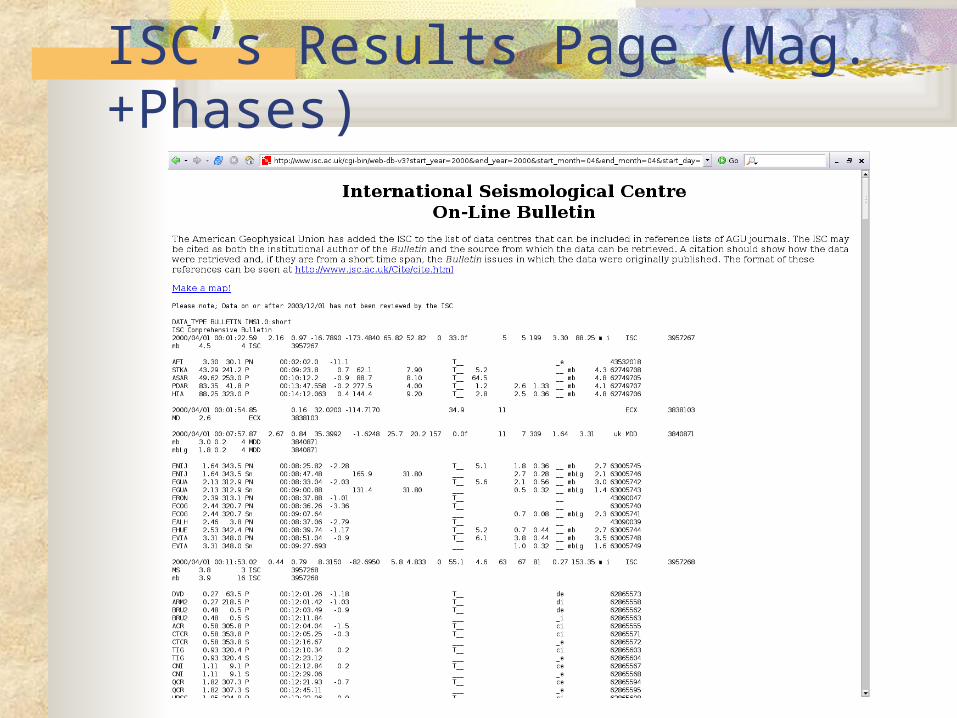
ISC’s Results Page (Mag.+Phases)

ISC’s Bandwidth Problems

Method – Analyzing the data

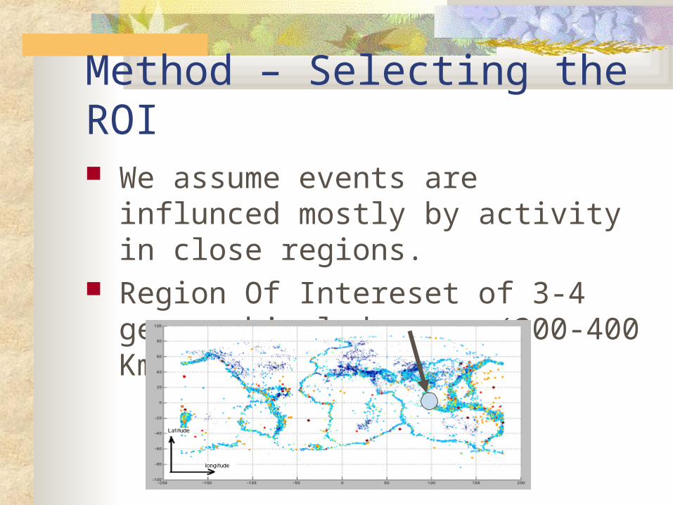
Method – Selecting the ROI We assume events are influnced mostly by

activity in close regions. Region Of Intereset of 3-4 geographical

degrees (300-400 Km) is chosen.

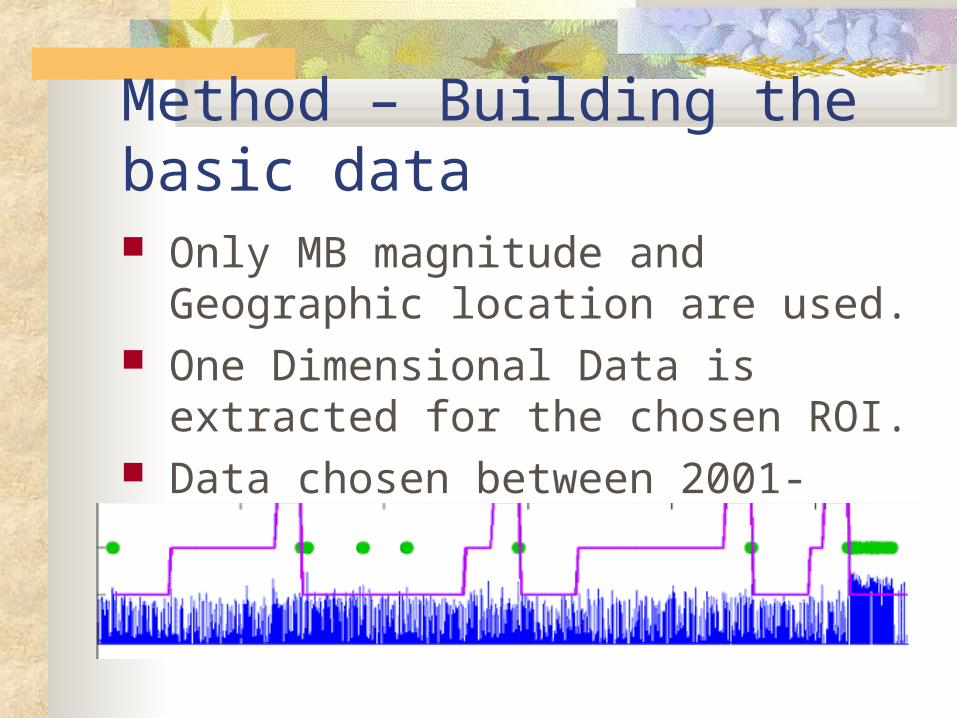
Method – Building the basic data Only MB magnitude and Geographic

location are used. One Dimensional Data is extracted for the

chosen ROI. Data chosen between 2001-2005.

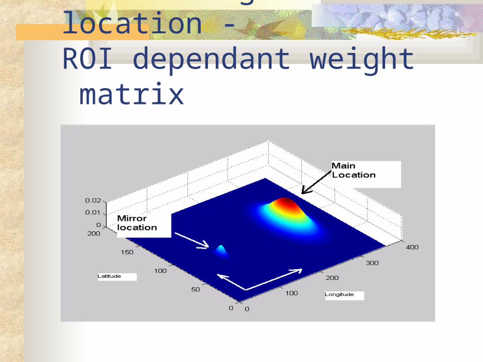
Considering the location - ROI dependant weight matrix

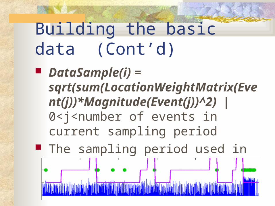
Building the basic data (Cont’d) DataSample(i) =

sqrt(sum(LocationWeightMatrix(Event(j))*Magnitude(Event(j))^2) | 0<j<number of events in current sampling period

The sampling period used in this project is 3600 seconds = 1 hour.

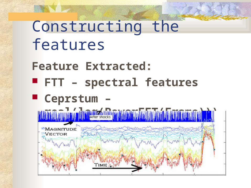
Constructing the featuresFeature Extracted: FTT – spectral features Ceprstum –real(log(PowerFFT(Frame)))

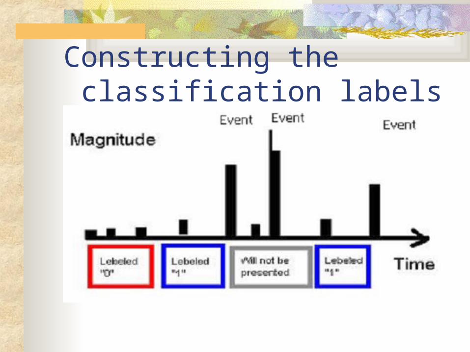
Constructing the classification labels

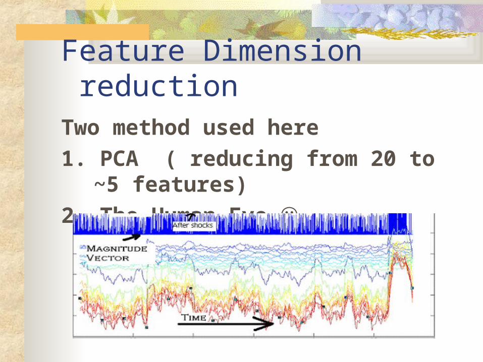
Feature Dimension reduction Two method used here

1. PCA ( reducing from 20 to ~5 features)

2. The Human Eye

Choosing the model5 classifiers were compared: Perceptron Expectation-Maximization – Gaussian

Mixture Models Radial Basis function Artificial neural network Support Vector Machine

Classifying Earthquakes Using SVM

Method The data was divided (after randomly

shuffling it) into two separate sets: A training set (75%) - Used for

constructing the classification model A testing set (25%) - Used for testing the

model The model was constructed using only the

training set, and tested on the testing set

Method (Cont’d) SVM has several variables which need to be set

prior to the model construction process, namely the kernel function and its associated parameters

Since RBF performed well on the data, and it is known as a generally good first pick, we chose it as our kernel function

Thus, there were two free parameters left for us to set

Method (Cont’d) Cross-validation on the training set was used in

order to evaluate various pairs of the parameters For each pair, the training set was divided into 5

different folds A SVM model was trained on four folds, and

tested on the fifth This process was repeated for each of the folds

(leave one out)

Method (Cont’d)

In order to test the model on a set it is not enough to measure the general accuracy of the model, that is, the number of vectors which the model had successfully labeled

Since there are more negative labeled vectors than positive ones, a trivial classifier which would label any vector as being negative could be evaluated as a relatively good classifier (with a record of over 80% success)

Thus, it is important to divide the resulting classification labels into four groups: True Positives, True Negatives, False

Positives and False Negatives

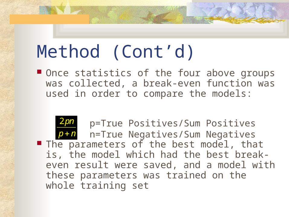
Method (Cont’d) Once statistics of the four above groups was

collected, a break-even function was used in order to compare the models:

The parameters of the best model, that is, the model which had the best break-even result were saved, and a model with these parameters was trained on the whole training set

p=True Positives/Sum Positivesn=True Negatives/Sum Negatives

2pn

p n

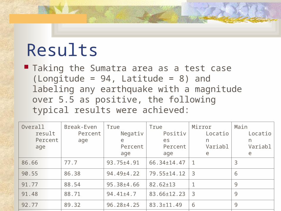
Results Taking the Sumatra area as a test case (Longitude

= 94, Latitude = 8) and labeling any earthquake with a magnitude over 5.5 as positive, the following typical results were achieved:

Main Location Variable

Mirror Location Variable

True Positives Percentage

True Negative Percentage

Break-Even Percentage

Overall result Percentage

3166.34±14.4793.75±4.9177.786.66

6379.55±14.1294.49±4.2286.3890.55

9182.62±1395.38±4.6688.5491.77

9383.66±12.2394.41±4.788.7191.48

9683.3±11.4996.28±4.2589.3292.77

12677±11.9995.39±485.2190.31

Results (Cont’d) Results show that SVM can classify the extracted

features quite well, achieving a record of 83.3%/96.28% (True Positive/True Negative)

This is quite surprising, considering the problem's nature

Further research could calibrate the variables more accurately, achieving even better results

The GUI

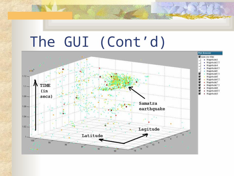
The GUI (Cont’d)

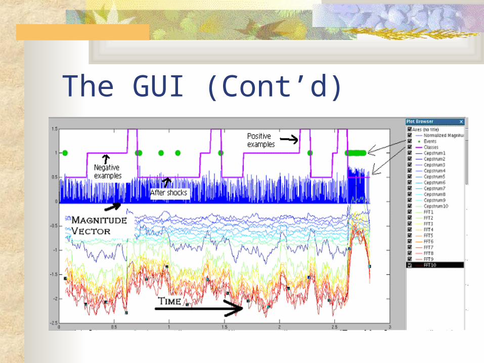
The GUI (Cont’d)

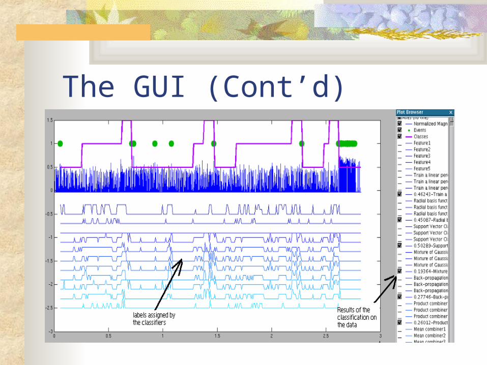
The GUI (Cont’d)

The GUI (Cont’d)