network reliability importance measures : combinatorics ... · network reliability importance...

Network reliability importance measures : combinatorics and Monte Carlo based computations

ILYA GERTSBAKH

Department of Mathematics Ben Gurion University

P.O.B 653 Beer Sheva 84105 ISRAEL

[email protected] YOSEPH SHPUNGIN

Department of Software Engineering Negev Academic College of Engineering and NMCRC

P.O.B 950 Beer Sheva 84100 ISRAEL

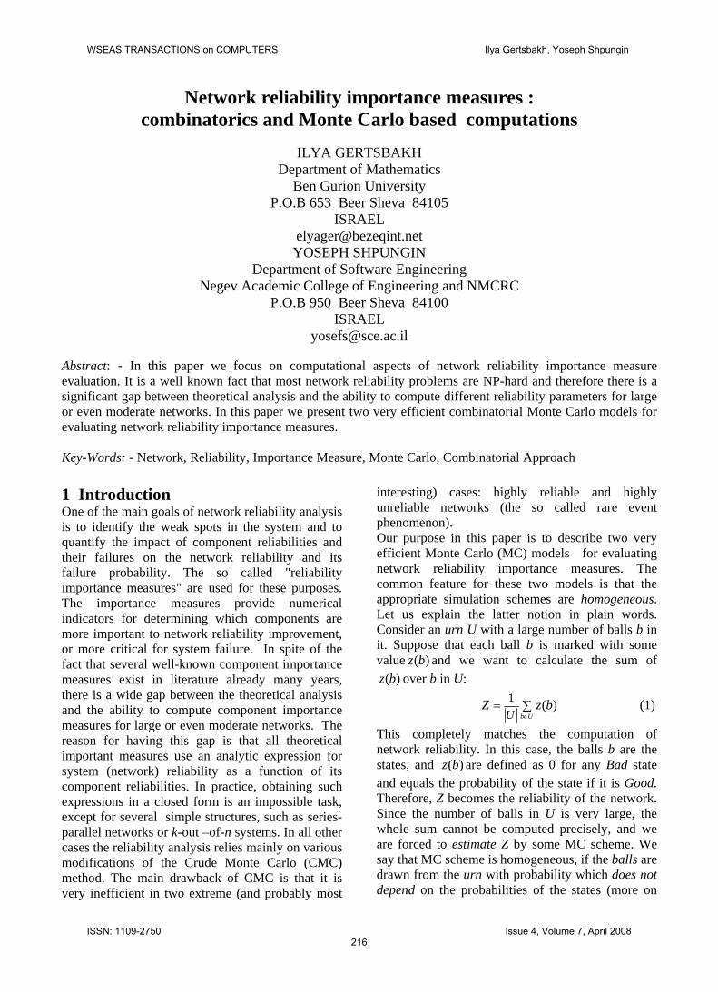
[email protected] Abstract: - In this paper we focus on computational aspects of network reliability importance measure evaluation. It is a well known fact that most network reliability problems are NP-hard and therefore there is a significant gap between theoretical analysis and the ability to compute different reliability parameters for large or even moderate networks. In this paper we present two very efficient combinatorial Monte Carlo models for evaluating network reliability importance measures. Key-Words: - Network, Reliability, Importance Measure, Monte Carlo, Combinatorial Approach 1 Introduction One of the main goals of network reliability analysis is to identify the weak spots in the system and to quantify the impact of component reliabilities and their failures on the network reliability and its failure probability. The so called "reliability importance measures" are used for these purposes. The importance measures provide numerical indicators for determining which components are more important to network reliability improvement, or more critical for system failure. In spite of the fact that several well-known component importance measures exist in literature already many years, there is a wide gap between the theoretical analysis and the ability to compute component importance measures for large or even moderate networks. The reason for having this gap is that all theoretical important measures use an analytic expression for system (network) reliability as a function of its component reliabilities. In practice, obtaining such expressions in a closed form is an impossible task, except for several simple structures, such as series-parallel networks or k-out –of-n systems. In all other cases the reliability analysis relies mainly on various modifications of the Crude Monte Carlo (CMC) method. The main drawback of CMC is that it is very inefficient in two extreme (and probably most

interesting) cases: highly reliable and highly unreliable networks (the so called rare event phenomenon). Our purpose in this paper is to describe two very efficient Monte Carlo (MC) models for evaluating network reliability importance measures. The common feature for these two models is that the appropriate simulation schemes are homogeneous. Let us explain the latter notion in plain words. Consider an urn U with a large number of balls b in it. Suppose that each ball b is marked with some value and we want to calculate the sum of

over b in U: ( )z b

( )z b

1 ( )b UU

Z z b∈

= ∑

( )z b

(1)

This completely matches the computation of network reliability. In this case, the balls b are the states, and are defined as 0 for any Bad state and equals the probability of the state if it is Good. Therefore, Z becomes the reliability of the network. Since the number of balls in U is very large, the whole sum cannot be computed precisely, and we are forced to estimate Z by some MC scheme. We say that MC scheme is homogeneous, if the balls are drawn from the urn with probability which does not depend on the probabilities of the states (more on

WSEAS TRANSACTIONS on COMPUTERS

Ilya Gertsbakh, Yoseph Shpungin

ISSN: 1109-2750216

Issue 4, Volume 7, April 2008

homogeneous schemes see in [1]). The important feature of homogeneous schemes is that the relative error is bounded (a basic example of a non-homogeneous scheme is the CMC and its variations). The paper is organized as follows. In Section 2, we give some basic notions and definitions. In Section 3, we present an efficient computation model [1,2] for evaluating reliability gradient vector, which is used for computing Birnbaum Importance Measure for a general case of networks with non-identical elements. As we mentioned above, our method allows obtaining numerical values of the component important measures without deriving the analytic expression for the network reliability function. In Section 4, we propose a highly efficient spectrum approach [3-5] for networks with identical components. It's worth noting that this approach provides easily implemented computations and allows obtaining, with minimal difficulties, various topological features of the network. Section 5 presents a series of numerical examples. 2 Basic notions and definitions 2.1 Network and its reliability All networks have vertices (nodes) and edges. There are many types of networks varying in their performance definitions and therefore with different concepts of their reliability. Let K-network be an undirected graph ( , , )N V E K= with a node-set V , an edge-set E and a set K V⊆ of special nodes called terminals. Also let | and ||V m= |E n= . In our model, nodes can never fail, while edges can. Note that all of our results are valid also for the case of reliable edges and unreliable nodes. If an edge fails, we say that it is down; otherwise we say it is up. By state of a network we call a binary vector 1( ,.., )nx x , where each component 1ix = if an edge is up and otherwise. Denote by

the network induced by its state, i.e. with the same node-set V and the edge-set consisting of all edges being up. A state of the network N is defined as being Good if any two terminals in the induced network are connected by some path of its edges. Otherwise it is Bad. The terminal connectivity criterion has the property of being monotone: each subset of a Bad state is a Bad state and each superset of a Good state is a Good state.

There are two network reliability models: static and dynamic. In this paper we restrict our attention to static networks. Each edge is associated with probability

ie 0ix =*N

*E

*N

ieip of being up and a probability

1iq ip= − of being down. We say that edges are identical if they all have the same probability of being up, that is for each i we havej≠ i jp p p= = . We define the network reliability 1( ,..., )nR R p p= as the probability that the network is in a Good state. 2.2 Reliability importance measures (IM's) IM's aim at quantifying the contribution of components to the measure of system performance, which in our case is system reliability. We present below a short description of several prevalent IM's proposed in literature. IM's were first introduced by Birnbaum [6]. The Birnbaum Importance Measure (BIM) of element is defined as ie

1( ,..., )B ni

i

R p pIp

∂=∂

(2)

It expresses the rate of increase of the network reliability with respect to the i-th element reliability increase.

Remark. For equal ip p≡ , first the derivatives i

Rp∂

∂

are computed and only afterwards all ip set to be equal p . Fussel and Vesely [7] later proposed another importance measure termed as Fussel-Vesely Importance Measure (FVIM):

1 1 1

1

( ,..., ,0, ,..., )1( ,..., )

FV i ii

n

nR p p p pIR p p

− += − (3)

It quantifies the decrement in system reliability caused by a particular component failure. Among other popular important measures let us note the following two: CIM and JIM. The Criticality Importance Measure (CIM) [8, 9] is a natural extension of BIM and includes the component unreliability whereas the BIM does not. The three above measures (BIM, FVIM and CIM) are functionally different and measure slightly different properties of system behavior, and one can infer different information from each one of them [10].These IM’s are united by the fact that quantify the importance rank of individual components. Contrary to them, the Joint Importance Measures (JIM's) quantify the importance of groups of components. They are very useful and have many applications [11, 12, 13]. Recently they became

WSEAS TRANSACTIONS on COMPUTERS Ilya Gertsbakh, Yoseph Shpungin

ISSN: 1109-2750217


popular in risk-informed applications [14, 15]. All the above mentioned IM’s are of universal nature with respect to the object of their application. Another direction is a more detailed study of IM's characteristics for specific systems. Recently, the most studied systems were the so called consecutive-k-systems [16, 17]. As a rule, the use of IM’s rests on the assumption that we have at our disposal the functional form of system reliability function. The fact that in practice we often don’t have this functional description, especially for complex systems, stimulated the interest in developing computational and numerical methods for evaluating IM's, see for example [18, 19, 20, 21]. These works, however, demand computing system reliability parameters. The method we develop in the present paper is based on system structural description and allows components ranking by their IM's without knowing the analytic form of the reliability function. 3 Using Reliability Gradient Vector for BIM evaluation 3.1 Gradient and border states The numerical evaluation of BIM will be done using some special properties of the reliability gradient vector. In this section we describe a special form of the gradient vector which allows using a highly efficient Graph Evolution Model [2] for its computation. Similar form of the gradient was outlined in [1]. Let us consider a monotone system [22] of n elements. Suppose that each element may be in two states: up with probability

ie

ip and down with probability . The state of a system is defined as a binary vector

iq1( ,.., )nx x , where each component

if is up and otherwise. All binary states are divided into two classes: Good and Bad.

1ix = ie 0ix = 2n

Definition 1. Reliability gradient vector R∇ is

defined as1

( ,..., )n

R RRp p∂ ∂∇ =∂ ∂

, i.e. component i of

the reliability gradient vector is the BIM of element . ie

Definition 2. System state is called direct neighbor or simply neighbor of state

if w differs from v in exactly one position (i.e. the Manhattan distance between vectors w and v equals 1). The set of all neighbor states of Bad is called the border set and is denoted

as DN*. Obviously,

1( ,..., )nw w w Bad= ∈

1( ,..., )nv v v Good= ∈

* .DN Bad⊆Surprisingly, it turns out that the reliability gradient vector is intimately related to the border states. To reveal this connection, we introduce an artificial evolution process on system elements. At 0t = all elements are down. Element is "born" after random time

ie~ exp( )i iτ λ , where iλ is chosen so that

the following equality takes place: ( 1) 1 i

i ip P e λτ −= ≤ = − . After the "birth", element remains up forever. Consider two system states

ie

1 1 1... ,...( , , ,0, , )i iv v v v v− + n= and . Suppose that at time t the system is in state v. We look for the probability that during a small time interval

1 1 1,( ,..., ,1, ..., )i i nw v v v v− +=

tΔ the system moves from v to w. Obviously, it will happen iff the element is born during this interval, and all other components which are in state 0 will not become alive during the same interval. The first event has probability

ie

( )i t o tλ ⋅Δ + Δ , and the second event has probability1 ( )o t− Δ . Then the probability that during [ , ]t t t+ Δ there will be the transition equals

v w→( )i t o tλ ⋅Δ + Δ . Let be a border state of the

system, i.e. v

*v DN∈ . Denote by the sum of ( )vΓ

iλ over the set of all indices i such that (0,...,1 ,...0)iv Good+ ∈ . Call the flow from v

into Good. Formally, ( )vΓ

*{ , (0,...,0,1 ,0,...,0) }( ) iv DN v Goodiv λ

∈ + ∈Γ = ∑ . We need two

other notations. Let 1( ( ),..., ( ))nR p t p t be the probability that the system is in Good state at the instant t. Let be the probability that the system is in state v at time t. Now let us consider the event "the system is in Good state at time t t

( ; )P v t

+ Δ ". This event takes place if at time t the system was already in the Good set or at time t it was in one of its border states and went during this interval from a border state to Good. All other possibilities which involve more than one transition during [ , ]t t t+ Δ have probability . Formally, ( )o tΔ

1( ( ),..., ( ))nR p t t p t t+ Δ + Δ

1*

( ( ),..., ( )) (=

; ) ( ) ( )v

nDN

R p t p t P v t v t o t∈

= + ⋅Γ ⋅Δ + Δ∑ .

Transfer 1( ( ),..., ( ))nR p t p t to the left-hand side, divide both sides by tΔ and set . We arrive at the following relationship:

0tΔ →

1

*

( ( ),..., ( )) ( ; ) ( )n

v DN

dR p t p t P v t vdt ∈

= Γ∑ . (4)

Now, represent the left-hand side of (4) in an alternative form:


ISSN: 1109-2750218


1

1

( )( ( ),..., ( )) n jn

j j

dp tdR p t p t dRdt dp dt

1( ( ) 1 , ( ) )

nt tj jj j

j j

dRp t e q t e q

dp j j

1 1{ ,..., }n nR q q . (5) Comparing (4) and (5) we arrive at the desired relationship between the gradient vector and the border state probabilities: 1 1

*{ ,..., } ( ; ) ( )n n

v DN

R q q P v t v (6)

From the latter formula we can get the expression for BIM of system elements in the following manner. It follows from the above proof that if we set 1 1{ ,..., }n nq q equal to{0,..., ,...,0}i iq , then we arrive at the following important formula:

{0,..., ,...,0}i i i ii

Rq R q

p *{ , (0,...,1 ,...,0) }

( ;1) iv DN v GoodiP v (7)

This relationship says that the sum of the probabilities of all border states which make a transition into the Good state by “activating” edge

is equal, up to a multiplier , to the BIM of component i.

ie iq

This formula will be the principal tool for the Monte Carlo evaluation of the gradient vector. Example 1. Let us take the network given in Fig. 1 and compute the BIM for edge e . The corresponding border states v such that

are: , ,. Then by (7) we get:

1

(1,0,0,0)v Good 1 (0,1,0,0)S 2 (0,1,1,0)S

3 (0,1,0,1)S

1 11

Rq

p= 1 1 2 3( ( ) ( ) ( )P S P S P S ) =

1 2 1 3 4 2 3 1 4 2 4 1 3( )p q q q p p q q p p q q .Dividing the both sides of the latter expression by 1 1q , we arrive at the BIM of .1e

The above example demonstrates computations via

formula (6). It is obvious that the main technical difficulty lies in identifying the border states and finding their probabilities. Computations similar to shown in the above example are difficult to carry out for large or even moderate networks. There exists, however a powerful computational Monte Carlo technique based on introducing a special scheme called Evolution and Merging process, which allows an efficient estimation of expressions of type (6). It was first suggested in the principal work [2].

3.2 Lomonosov's turnip To make the appropriate Monte Carlo scheme for evaluating BIM more transparent, we give here a short description of the Evolution and Merging process (EMP or Lomonosov's turnip) [1] which will be adopted to our needs. Let us consider the case of unreliable edges and reliable nodes The EMP uses two basic ideas. The first one is introducing an artificial random process associated with each edge. The second is defining the trajectories of a random process built on network states. Introduce now for each edge an artificialcreation process, as it was described above in 3.1. Remind that the probability of being down at 0 1tfor each edge coincides with the static down-probability . At ( )q e 0t the network is in Bad set (there are no edges). Denote by ( )N network's "birth" time, i.e. at random instant ( )N the network becomes Goodand remains Good forever. Let us denote by { ( ) 1}P N the probability that at moment 0 1tin the creation process the network is Good.Then we have:

N

( ) { ( ) 1}R N P N (8) In words: the static probability ( )R N that the network is Good coincides with the probability that in the edge creation process network state is Good at the instant t0 1

3eS, i.e. N enters the Good set before

or at 0 1t . On Fig. 2 we present the creation process for the network of Fig 1. The operational criterion is the two terminal connectivity with terminal nodes S and T.

4e1e

Initially all edges are in the down state (the zerolevel of the turnip). The first level shows all possible evolution results from the zero level which appear as a result of a birth of a single edge. There are four such states. The second level of the turnip showswhat happens when a second edge is born. We

2e T

Fig. 1


ISSN: 1109-2750219


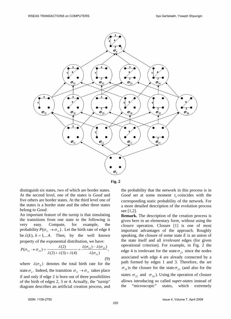
Fig. 2 distinguish six states, two of which are border states. At the second level, one of the states is Good and five others are border states. At the third level one of the states is a border state and the other three states belong to Good. An important feature of the turnip is that simulating the transitions from one state to the following is very easy. Compute, for example, the probability 11 21(P )σ σ→ . Let the birth rate of edge k be ( ), 1,...4k kλ = . Then, by the well known property of the exponential distribution, we have:

11 2111 21

11

( ) ( )(2)( )

(2) (3) (4) ( )P

λ σ λ σλσ σ

λ λ λ λ σ−

→ = =+ +

,

(9) where )( ijσλ denotes the total birth rate for the state .ijσ Indeed, the transition 11 21σ σ→ takes place if and only if edge 2 is born out of three possibilities of the birth of edges 2, 3 or 4. Actually, the "turnip" diagram describes an artificial creation process, and

the probability that the network in this process is in Good set at some moment t coincides with the corresponding static probability of the network. For a more detailed description of the evolution process see [1,2].

0

Remark. The description of the creation process is given here in an elementary form, without using the closure operation. Closure [1] is one of most important advantages of the approach. Roughly speaking, the closure of some state E is an union of the state itself and all irrelevant edges (for given operational criterion). For example, in Fig. 2 the edge 4 is irrelevant for the state 21σ since the nodes associated with edge 4 are already connected by a path formed by edges 1 and 3. Therefore, the set

31σ is the closure for the state 21σ (and also for the states 22σ and 24σ ). Using the operation of closure allows introducing so called super-states instead of the “microscopic” states, which extremely


ISSN: 1109-2750220


accelerates the evolution process on turnip. For instance, if we have a network with 100 vertices and 2000 edges, using the super-states will result in a trajectory of maximal length 99. Without the closure operation the maximal length can be up to 2000. Consider a random process ( )tσ whose states are the states of the described creation process. It was proved in [1] (for the super-states too) that (i) ( )tσ is a Markov process; (ii) The time spent by ( )tσ in a particular state σ ′ is distributed as exp( ( ))λ σ ′ . Define now a trajectory, which plays the central role in the described process and in the corresponding Monte Carlo scheme. Definition 3. A trajectory is a sequence

0 1( , ,..., )ru σ σ σ= of states such that 0σ is the initial trivial state, each iσ is the direct successor of 1iσ − , and rσ is the first state belonging to Good. For example, the sequence 0 11 21 31 4( , , , , )σ σ σ σ σ on the Fig. 2, is a trajectory. Now, in terms of the trajectories, the network is Good at moment t if there exists at least one trajectory that reaches Good before t. It is easy to calculate the probability p(u) of the trajectory :u . (10)

1

10

( ) ( )r

i ii

p u P σ σ−

+=

= →∏

Denote by the probability that the Good state will be reached before time t given that the creation process goes along trajectory u. Then by the above mentioned property, the process is sitting in each state

( | )P t u

jσ an exponentially distributed random time ( )jτ σ . Due to the Markov property, the total time

along the trajectory u is a sum of the respective independent random variables, and 0 1( | ) ( ( ) ... ( ) | ).rP t u P t uτ σ τ σ −= + ≤ (11) Note that is a convolution and can be computed analytically [1] or simulated [23]. Now the probability that at moment t the creation process reaches Good equals:

( | )P t u

( ) ( ( ) ) ( ) ( | ),u U

R N P N t p u P t uξ∈

= ≤ = ⋅∑ (12)

where U is the set of all trajectories. The expression (12) has the form of an expectation and opens the way to estimating ( )R N by means of a Monte Carlo algorithm described in [1,2]. 3.3 Numerical evaluation of BIM's Let us now use the turnip for evaluating BIM. Remind that by the formula (6) we have

1 1*

{ ,..., } ( ) ( )n nv DN

R q q P v vλ λ∈

∇ ⋅ = Γ∑ ,

or using the turnip notations :

1 1*

{ ,..., } ( ) ( )n n jDNj

R q q P vσ

λ λ σ∈

∇ ⋅ = ∑ Γ , (13)

where *{ , (0,...,0,1 ,0,...,0) }( ) iDN v UPj iv

σλ

∈ + ∈Γ = Σ . Now, for each

border state σ we have following formula: ( ) ( ( ) 1) ( ( ) 1).P P P Nσ ξ σ ξ= ≤ − ≤

Here the first term is the probability that the creation process is at 0 1t = in the state σ or is in Good. The second term is the probability that the Good state was reached before . The difference is therefore the desired probability that at

0 1t =

0 1t = the process is inσ . Considering all trajectories leading from 0σ into Good, we obtain the following formula:

0 0( ) ( )( ( ( ) | ) ( ( ) | ).u U

P p u P t u P N t uσ ξ σ ξ∈

= ≤ − ≤∑

Substituting the latter expression into (13), we get: 1 1

*

0 0*

{ ,..., } ( ) ( )

( )( ( ( ) | ) ( ( ) | ) ( ).

n n jDNj

ju UDNj

R q q P v

p u P t u P N t uσ

σ

λ λ σ

ξ σ ξ∈

∈∈

σ

∇ ⋅ = Γ =∑

≤ − ≤ Γ∑ ∑

Changing the order of summation we arrive at the following formula:

1 1{ ,..., }n nR q qλ λ∇ ⋅ =

( , ),

(14)

1 such that ( )

( ( )m

ii u U e ui

p u f uσ

λ σ+= ∈ ∈

⋅∑ ∑

where ( )uσ is the border state defined by the trajectory , u ( )uσ + is a set of all edges which "transfer" ( )uσ to the Good state and ( , )f uσ =

0 0( ( ) | ) ( ( ) | )P t u P N t uξ σ ξ≤ − ≤ . The sum in (14) has the form of the expectation, which is the key for Monte Carlo numerical procedures on the turnip. We use the following simulation scheme to evaluate BIM's values simultaneously for all network edges. Define by ArB an array of size n so that ArB[i] will denote the BIM of edge i. Simulation scheme. Step1. Put [ ] 0, 1 .ArB i i n= ≤ ≤ Step2. Generate trajectory u leading from the trivial state to the state in Good. Step3. Let jσ be a border state on this trajectory and let edge ( )i je uσ +∈ . Then

0 0[ ] [ ] ( ( ( ) | ) ( ( ) | ).jArB i ArB i P t u P N t uξ σ ξ= + ≤ − ≤ Step4. Repeat steps 2 and 3 K times. Step5. For all i (1 i n≤ ≤ ) put [ ] [ ]/ .ArB i ArB i K=(For the calculation of the difference of two


ISSN: 1109-2750221


convolutions (Step 3 ) see [1] and [11]). 4 Spectral approach to computing network reliability importance measures In this section we will derive the BIM and the FVIM for networks with identical elements by means of so called network combinatorial spectrum. This notion was introduced in [3] and [4,5] to estimate network lifetime distribution and /or its static reliability. For reader’s convenience we remind shortly the principal idea of network combinatorial characteristic called spectrum. For simplicity we demonstrate the method for the case of reliable nodes and unreliable edges. It was shown in [4] that this approach is applicable also to the case of reliable edges and unreliable nodes, or – which is more complicated – to the case of both unreliable nodes and edges. Let EΠ be the set of all edge permutations in E. Let π be a particular permutation. By sub-permutation

(1... )iπ of π we denote a sequence constructed of the first i edges in π . For each sub-permutation (1... )iπ we define a network state ( (1... ))S iπ , where all the edges in (1... )iπ are up and all other edges in π are down. For each edge

je and permutation π denote by ( )jeπ the index of this edge in π . Example 2. Let us take the network in Fig.1 and let our permutation be (1,3,2,4)π = . Then, for example,

(1...3) (1,3,2)π = and ( (1...3))S π is a state in which edges 1,3,2 are up, and edge 4 is down. We have also: 1( ) 1eπ = , 2( ) 3eπ = , 3( ) 2eπ = , 4( ) 4eπ = . Next we define an anchor. This notion plays a central role in our reasoning. Definition 4. Let ( )r r π= be the first index in permutation π so that ( (1... ))N rπ is Good. We say that ( )r π is the anchor of the permutation π . Definition 5. Denote by ix the number of all permutationsπ such that is the anchor ofi π . We say that the set

SP={{ },1 }ix i n≤ ≤ (15) is the combinatorial spectrum of the network. Example 3. We demonstrate these definitions on a network given in Fig. 1. The total number of permutations of 4 edges in the network is 24. Let

(3,1,2,4)π = . We see that the first index such that the network state becomes Good is 3. Therefore

( ) (3,1,2,4) 3r rπ = = is the anchor of this permutation. After going over all permutations we arrive at the following combinatorial spectrum of the given network: i | 1 2 3 4 ix | 0 4 14 6 It was shown in [4] that given a network spectrum

{{ },1 }iSP x i n= ≤ ≤ , the network reliability may be expressed in the following form:

1 ! ( )!

i n in n

rr i r

p qR xi n i

−

= =

⋅= ∑ ∑⋅ −

(16)

In our example, the network reliability is: 4 4

1 ! (4 )!

i n i

rr i r

p qR xi i

−

= =

⋅= =∑ ∑⋅ −

4 3 23p p q p q+ ⋅ + ⋅ 2 .

Remark. Sometimes it is more convenient to use the cumulative form of the spectrum: *

1{ : ,1 }

i

i i ik

SP y y x i n=

= = ≤ ≤∑ (17)

The value expresses the number of permutations iyπ such that ( )r iπ ≤ , or, in other words, that

( ( ))N iπ is Good. Example 4. For the network on Fig. 1, we have from the above example that there are 14 permutations with anchor and 4 permutations with anchor

3r =2r = . So, we get . 3 18y =

It is easy to check from (16) that in the case of the cumulative spectrum the network reliability is given by

1 ! ( )!

i n in

ii

p qR yi n i

−

=

⋅= ⋅∑⋅ −

(18)

Clearly, in the case of large or moderate networks we can not get the exact values of the spectrum. We can however try to estimate them by a Monte Carlo simulation [3,4]. It is worth to mention the main advantages of this combinatorial approach: (a) eliminating the rare event phenomenon. This fact results in bounding the relative error, so the method is especially efficient for highly reliable networks. (b) once computed, the combinatorial spectrum serves for as many values of nodes or edge failure probabilities as needed. (c) possibility to use for solving different reliability problems in dynamic networks. Definition 6. Denote by the number of all permutations

,i jzπ such that ( (1... ))S iπ is Good and

( )je iπ ≤ . We call the set - the BIM spectrum.

,{ ,1 ,1 }i jz i n j≤ ≤ ≤ ≤ n

Definition 7. Denote by the number of all permutations

,i jvπ such that ( (1... ))S iπ is Good and


ISSN: 1109-2750222


( )je iπ > .We call the set -

the FVIM spectrum. ,{ ,1 ,1 }i jv i n j≤ ≤ ≤ ≤ n

We see from these definitions that . , ,i j i j iz v y+ =

i 1y ,1iz ,2iz ,3iz ,4iz 1 0 0 0 0 0 2 4 4 4 0 0 3 18 12 18 12 12 4 24 24 24 24 24

Table 1

Example 5. Let us take the edge from the network in Fig. 1 and let us compute . It is easy to see that there are 6 permutations

1e

3,1zπ such that

( (1...3))S π is Good and 1( ) 3eπ > . So we get . From the previous example, 3 3,1 6y z− = 3 18y = .

Hence, we get that . The BIM spectrum for the network is given in Table 1.

3,1 12z =

Claim 1. (a) The BIM for edge j is given by the following formula:

1 1

, ,

1

( )! ( )!

i n i i n in i j i i jB

ji

z p q y z p qI

i n i

− − − −

=

⋅ ⋅ − − ⋅ ⋅= ∑

⋅ − (19)

(b) The FVIM for edge j is given by the following formula:

1

,

1

11( ) ! ( )!

i n in i jFV

ji

v p qI

R p i n i

− −

=

⋅ ⋅= − ∑

⋅ − (20)

Proof. (a) Remind that BIM for edge je equals

1 1( ,...1 ,..., ) ( ,...,0 ,..., )j n jj

RnR p p R p

p∂ = −∂

p

(see[12 ]). The value , by the definition 5, is the number of permutations

,i jzπ such that ( (1... ))S iπ is Good and the

edge je is up. For fixed permutationπ the probability of an appropriate state with je being up, equals . Take into account that a specific state with i edges being up and n-i edges being down we obtain times (from different permutations). Then the summary probability of all Good states with i edges being up and n-i edges

being down equals

1i np q− ⋅ i−

! ( )!i n i⋅ −

1,

! ( )!

i ni jz p qi n i

− −⋅ ⋅

⋅ −

i

. For the case of

the edge je being down we get the expression of the

appropriate probability as 1

,( )! ( )!

i n ii i jy z p q

i n i

− −− ⋅ ⋅

⋅ −, and

(a) follows. (b) Using (a), the definition of FVIS and the above mentioned fact that , ,i j i j i jz v y ,+ = we arrive at the desired expression. In order to rank the elements according to their importance measure there is no need to compute the partial derivatives. The following simple claim takes place. Claim 2. Let { ,1 }ijz i n≤ ≤ and be the BIM spectrum elements for the edges

{ ,1 }isz i n≤ ≤

je and se respectively. Then: (a) If for all 1 i n≤ ≤ the inequality holds,

then

ij isz z≥

j s

R Rp p∂ ∂≥∂ ∂

. Moreover, if for at least one index

i a strong inequality holds, thenij isz z>j s

R Rp p∂ ∂>∂ ∂

.

(b) Suppose that the condition of (a) does not take place. Then let be the maximal index such that

kij isz z≠ . Suppose that . Then there exists

some valuekj ksz z>

0p such that for all 0p p≥ the inequality

j s

R Rp p∂ ∂>∂ ∂

holds.

Proof. (a) From (12) we have:

j s

R Rp p∂ ∂− =∂ ∂

1 1

, ,

1

( )! ( )!

i n i i n in i j i i j

i

z p q y z p qi n i

− − − −

=

⋅ ⋅ − − ⋅ ⋅−∑

⋅ −

1 1, , , ,

1

( ) ( )! ( )!

i n i i n in i j i s i s i j

i

z z p q z z p qi n i

− − − −

=

− ⋅ ⋅ − − ⋅ ⋅=∑

⋅ −

1 1, ,

1

( )! ( )!

i n in i j i s

i

z z p qi n i

− − −

=

− ⋅ ⋅∑

⋅ − and (a) follows.

(b) From the definition of k and the latter expression we obtain:

1 1, ,

1

( )! ( )!

i n ik i j i s

i

z z p qi n i

− − −

=

− ⋅ ⋅=∑

⋅ −

, ,1 1

1

( )( (

! ( )!k i j i sk n k k i

i

z z qp qi n i p

− − − −

=) )

−⋅ ⋅ ⋅∑

⋅ − and for ,

the assertion follows.

1p →

We use the following Monte Carlo scheme to obtain unbiased estimates for the , and . iy ,i jz ,i jvSimulation scheme. Step1. Initialize all , and to be 0. ia ,i jb ,i jcStep2. Simulate the permutationπ ∈Π . Step3. Find ( )r r π= - the minimal index of edge inπ so that the state ( (1... ))N rπ is Good.


ISSN: 1109-2750223


Step4. Let . : 1r ra a= +Step5. For all j such that ( )je rπ ≤ let . , ,: 1r j r jb b= +Step6. For all s such that ( )se rπ > let . , ,: 1r s r sc c= +Step7. Let . If Go to Step4. : 1r r= + r n≤Step8. Repeat steps 2-7 M times.

Computing , ,, ,

! !!ˆ ˆˆ, ,i j i jii i j i j

b n c na ny z vM M M

⋅ ⋅⋅= = = we

can from (18), (19), (20) obtain, respectively, the unbiased estimates for R , BI and FVI . 5 Numerical examples In this section we present several examples, which explain how we can rank network elements (edges and nodes) in accordance to their BIM's by using spectrum approach. For this purpose we choose some hypercubes (note that hypercube configurations are widely used in computer networks [24]). Example 6. Consider a four-terminal hypercube with =16 nodes and 32 edges. This hypercube is shown on Fig. 2. Let its terminals be nodes 1, 8, 9 and 16. Edges will be denoted by (k,s) , where k and s are node numbers.

4H42

Fig. 3 Table 2 presents a fragment of simulation results, based on replications. By we marked the simulated value of spectrum and by - the

simulated value of BIM spectrum

410 ia

,( , )i k sbBIS for edge (k,s).

Remind that for edge ranking there is no need to compute their BIM's. We see from Table 2 that the values of BIS for edges (1,9) and (8,16) are very close to each other. On the other hand, these values are consistently greater than the BIM spectrum values for edge (1,2) and the latter – than those of (3,4). So, we rank the edges by their importance in

the following order (read table 2 in horizontal direction) (1,9) (8,16) (1,2) (3,4)= > > .

i ia ,(1,9)ib ,(8,16)ib ,(1,2)ib ,(3,4)ib 6 2 2 1 0 1 7 15 14 14 2 3 8 59 51 50 12 12 9 154 129 128 40 38 10 350 286 267 109 91 11 679 501 492 235 206 12 1333 886 904 525 438 13 2385 1478 1492 996 892 14 3723 2187 2210 1625 1547 15 5230 3012 3042 2502 2363

Table 2

Note that from the whole data array (not presented here) one can infer that in our network there are three, by their BIM's, different groups of edges. The first consists of edges (1,9) and (8,16), which connect the pairs of terminals. The second is the group consisting of all other edges incident to one of the terminals 1, 8, 9 and 16, and the third – all other edges. The edges within each group have equal BIM’s, the first group dominates the second, and the second dominates the third. This conclusion may seem to be intuitively obvious, but for the same hypercube with nonsymmetrical terminals, or for other nonsymmetrical networks, similar conclusions are not so obvious. More involved cases may need to use special statistical analysis for better discrimination between edges with close BIM’s spectra.. Example 7. Consider now the same hypercube, but with three terminals: 1, 10 and 16. Table 3 presents a fragment of simulation results, based on replications. The notation is the same as in the Table 2. This case is less obvious due to the non-symmetrical terminals. We can, by the results, rank the edges in the following order: (1,9)>(9,10)>(8,16)>(3,4)>(7,8). (A simulation run with 100,000 replications leads to the same conclusion). An interesting feature of the data in Table 3 is that here we can not unite in one group (as it was in Example 6) all edges incident to one of the terminals. For example, edge (1,9) is ranked higher than the edge (9,10). Note also that there exist edges which are not incident to any terminal and do not belong to one rank group (this was not

410


ISSN: 1109-2750224


the case of the previous example). Such edges, for example, are (3,4) and (7,8).

i ia ,(1,9)ib ,(9,10)ib ,(8,16)ib ,(3,4)ib ,(7,8)ib

6 13 11 11 2 0 2 7 41 33 29 8 5 4 8 99 78 72 37 23 20 9 193 163 159 93 79 68 10 322 311 310 208 167 150 11 547 583 553 441 356 320 12 795 970 923 818 660 614 13 1195 1576 1527 1416 1173 1123 14 1351 2288 2234 2151 1845 1777 15 1435 3027 3033 2969 2681 2590

Table 3

Example 8. Our initial hypothesis was that the type of inequality between BIM's of two elements remains unchanged for all values of i (see Claim 2(a)). We'll see from the following example that it is not so. Consider the same hypercube with three terminals: 1, 10, 16, but with reliable edges and unreliable nodes. (Remind that the terminal nodes are supposed to be reliable). Table 4 presents the results (also based on replications). As it is seen from this table, the nodes 2, 9 and 15 are ranked as follows: (2) = (9)>15. It is interesting that all these three nodes are the "neighbors" of terminals, but the node 15 is less important than the first two.

4H

410

i ia ,(2)ib ,(9)ib ,(15)ib ,(7)ib ,(6)ib 6 1161 800 805 208 140 208 7 2045 1712 1718 964 837 812 8 2483 2926 2926 2307 2088 1986 9 2052 4161 4165 3821 3569 3497

10 1097 5200 5204 5038 4889 4871 11 450 6091 6088 6028 5970 5964 12 158 6912 6904 6894 6909 6879 13 49 7696 7694 7688 7694 7692 14 0 8460 8460 8458 8465 8459 15 0 9232 9228 9227 9230 9228

Table 4

Let us now pay attention to the last two columns, related to nodes 7 and 6. We see that , but for all the inequalities become reversed. We have checked this fact by increasing the number of simulation replications and got the same results.

We have also combinatorial explanation: the number of short paths is greater for node 6, but the number of longer paths is greater for node 7. Here the conditions of the Claim 2(b) hold and therefore starting with some

1,(7) 1,(6)b b<

1i >

0p , node 7 is more important than node 6. Example 9. One of the important characteristics of Monte Carlo computations is the convergence rate of parameter estimates to their true values. Numerous simulation experiments reveal that the estimates of component importance rapidly become stable and change very little as the number of simulation runs increases. For example, BIM’s were estimated for a hypercube with 128 nodes (5 of them were terminals) and 448 edges . Nodes are subject to failures and edges are reliable. Table 5 presents the estimated BIM's spectrum for node 2, divided by number of replications K, for K= ,

, ,see columns 2,3,4, respectively.

7H

410510 610

i 4

,(2) /10ib 5,(2) /10ib 6

,(2) /10ib

20 0 0 0.00005 30 0.01500 0.01610 0.01854 40 0.13500 0.13270 0.13559 50 0.29900 0.28900 0.29929 60 0.41300 0.41660 0.42126 70 0.51200 0.51400 0.51752 80 0.60100 0.60650 0.60722 90 0.69400 0.68610 0.69079 100 0.76500 0.77090 0.77191 110 0.84400 0.85160 0.85211 120 0.93800 0.93430 0.93405 125 0.97500 0.97580 0.97583

Table 5

6 Conclusions (1) We have developed a new method of computing network component importance measures, for networks with different component reliabilities. (We deal with Birnbaum importance measure-the BIM). Our method is based on a connection between the so-called border state probabilities and the reliability gradient vector. The network component importance measures are the coordinates of the reliability gradient vector. Using a specially constructed evolution process on the network components, we have developed an efficient numerical procedure for estimating the border state probabilities and obtaining, therefore, the BIM’s. Our numerical procedure avoids the rare event phenomenon and


ISSN: 1109-2750225


allows obtaining all gradient coordinates in one simulation run. (2) For the case of networks with equally reliable components (nodes, or edges or both), we have developed a new efficient computation scheme for evaluating the BIM’s. Its main idea is based on calculating, via a Monte Carlo scheme, network combinatorial invariant called spectrum and on the connection between the spectrum and the component BIM’s. Spectrum based BIM computations allow obtaining results without calculating the gradient vector. (3) The techniques developed in this paper can be viewed as a first step toward developing an algorithm for optimal network reliability design, since the latter has to be based on computing network reliability gradient vector. References: [1] T. Elperin, I. Gertsbakh, M. Lomonosov, An

evolution model for Monte Carlo estimation of equilibrium network renewal parameters, Probability in the Engineering and Informational Sciences, Vol. 6, 1992, pp. 457-469.

[2] T. Elperin, I. Gertsbakh, M. Lomonosov, Estimation of network reliability using graph evolution models, IEEE Transactions on Reliability, Vol. 40, No.5, 1991, pp. 572-581.

[3] Gertsbakh and Y. Shpungin, Combinatorial approaches to Monte Carlo estimation of network lifetime distribution, Appl. Stochastic Models Bus. Ind., Vol 20, 2004, pp. 49-57.

[4] Y. Shpungin, Combinatorial Approach to Reliability Evaluation of Network with Unreliable Nodes and Unreliable Edges, International Journal of Computer Science, Vol.1, No.3, 2006, pp. 177-183.

[5] Y. Shpungin, Networks with unreliable nodes and edges: Monte Carlo lifetime Estimation, International Journal of Applied Mathematics and Computer Sciences, Vol. 4, No. 1, 2007, pp. 168-173.

[6] Z. W. Birnbaum, On the importance of different components in a multicomponent system, Multivariate Analysis 2, New York, Academic Press, 1969.

[7] J. Fussel, How to calculate system reliability and safety characteristics, IEEE Transactions on Reliability, Vol. 24, No.3, 1975, pp. 169-174.

[8] F. C. Meng, Comparing the importance of system elements by some structural

characteristics, IEEE Transctions on Reliability, Vol 45, No 1, 1996, pp. 59-65.

[9] L. M. Leemis, Reliability – Probabilistic models and Statistical Methods, Prentice Hall, Inc, 1995.

[10] J. F. Espiritu, D. W. Coit and U. Prakash, Component Criticality Importance Measures for the Power Industry, Electric Power Systems Research, Vol. 77, Issues 5-6, 2007, pp. 407-420.

[11] E. Zio and L. Podofillini, Accounting for components interactions in the differential importance measure, Reliability Engineering & System Safety, Vol. 91, Issues 10-11, 2006, pp. 1163-1174.

[12] J.S. Hong and C. H. Lie, Joint reliability-importance of two edges in an undirected network, IEEE Trans. on Reliab., Vol. 42, No.1, 1993, pp. 17-23.

[13] M. J. Armstrong, Joint reliability-importance of elements, IEEE Trans. on Reliab., Vol. 44, No. 3, 1995, pp 408-412.

[14] Bogronovo E., Apostolakis G. E., A new importance measure for risk-informed decision making, Reliab. Eng. And Sys. Safety, Vol. 72, 2001, pp. 193-212.

[15] Youngblood R. W., Risk significance and safety significance, Reliab. Eng. And Sys. Safety, Vol. 73, 2001, pp. 121-136.

[16] Hsun-Wen Chang, Jun-Da Chen, Joint Structural Importance in Consecutive-k- Systems, Proceedings of 7th WSEAS International Conference on Applied Computer Science, 2007, pp. 95-100.

[17] H. W. Chang, R. J. Chen and F. K. Hwang, The structural Birnbaum importance of consecutive-k systems, Journal of Combinatorial Optimization, Vol. 6, 2002, pp. 183-197.

[18] Yung-Ruei Chang, Amari S.V, Sy-Yen Kuo, OBDD-based evaluation of reliability and importance measures for multistate systems subject to imperfect fault coverage, IEEE Transactions on Dependable and Secure Computing, Vol. 2, Issue 4, 2005, pp. 336-347.

[19] Bogronovo E., Differential, criticality and Birnbaum importance measures: An applicationn to basic event, groups and SSCs in event trees and binary decision diagrams, Reliability Engineering & System Safety, Vol. 92, Issue 10, 2007, pp. 1458-1467.

[20] Hae Sang Lee, Chang Hoon Lie, Jung Sik Hong, A computation method for evaluating importance measures of gates in a fault tree,


ISSN: 1109-2750226


IEEE Transactions on Reliability, Vol. 46, Issue 3, 1997, pp. 360-365.

[21] G. Rubino, Sensitivity analysis of network reliability using Monte Carlo, Proceedings of the 37th conference on Winter simulation, Orlando, Florida, 2005, pp. 491-498.

[22] I. Gertsbakh, Reliability Theory with Applications to Preventive Maintenance, Springer, 2000.

[23] I. Gertsbakh and Y. Shpungin, Product-Type Estimators of Convolutions, Semi-Markov Models and Applications, Kluwer Academic Publishers, 1999, pp. 201-206. [24] M. Mitzenmacher, E. Upfal, Probability and Computing . Randomized Algorithms and Probabilistic Analysis, Cambridge University Press, 2005.


ISSN: 1109-2750227


network reliability importance measures : combinatorics ... · network reliability importance...

Documents