network model of flow, transport and biofilm effects in porous media

Transport in Porous Media30: 1–23, 1998. 1© 1998Kluwer Academic Publishers. Printed in the Netherlands.

Network Model of Flow, Transport and Biofilm

Effects in Porous Media

BRIAN J. SUCHOMEL1, BENITO M. CHEN2,? and MYRON B. ALLEN III21Institute for Mathematics and its Applications, University of Minnesota, Minneapolis,Minnesota, U.S.A.2Department of Mathematics, University of Wyoming, Laramie, WY 82071, U.S.A.

(Received: 22 November 1996: in final form: 29 July 1997)

Abstract. In this paper, we develop a network model to determine porosity and permeability changesin a porous medium as a result of changes in the amount of biomass. The biomass is in the formof biofilms. Biofilms form when certain types of bacteria reproduce, bond to surfaces, and produceextracellular polymer (EPS) filaments that link together the bacteria. The pore spaces are modeledas a system of interconnected pipes in two and three dimensions. The radii of the pipes are given bya lognormal probability distribution. Volumetric flow rates through each of the pipes, and throughthe medium, are determined by solving a linear system of equations, with a symmetric and positivedefinite matrix. Transport through the medium is modeled by upwind, explicit finite differenceapproximations in the individual pipes. Methods for handling the boundary conditions betweenpipes and for visualizing the results of numerical simulations are developed. Increases in biomass,as a result of transport and reaction, decrease the pipe radii, which decreases the permeability ofthe medium. Relationships between biomass accumulation and permeability and porosity reductionare presented.

Key words: biofilm, network model, permeability, transport, numerical diffusion.

1. Introduction

Biofilms, complexes of bacterial biomass and extracellular polymer, have a varietyof interesting effects when they grow in porous media. Typically, the presence ofbiofilms in the voids of a porous medium reduces its permeability and porosity. Thisfact suggests a wide range of applications in the control of groundwater contaminanttransport and production from oil reservoirs. This paper presents a network modelof fluid flow and the transport and growth of biofilms in a porous medium.

There is a fundamental difficulty in modeling the effects of biofilm growth andtransport in porous media: the microscopic dynamics, best understood at the scale ofindividual pores, affect macroscopic flow properties such as permeability and poros-ity, which are meaningful on much coarser scales. This is thescale-upproblem. Thepurpose of our model is to help scale up from a simplified but reasonable representa-tion of the microscopic physics to the scale described by macroscopic flow properties.The macroscale we model is in the order of a soil column in a lab. At this scale, soilsamples are fairly homogenous but have heterogeneous microstructure typical of the

2 BRIAN J. SUCHOMEL ET AL.

pore scale. The scaling up to the level of field tests is a different task, which we donot attempt.

Several researchers have studied biofilms and their effects on porous media. Van-deviver and Baveye (1992) experimentally investigated a relationship between trans-port and clogging for biofilms. Other researchers, including Tanet al. (1994) andLindqvist et al. (1994), developed models of porous media based on the continuumhypothesis, including transport and sorption of bacteria, and used physical experi-ments to test their models. Taylor and Jaffe (1990a,b,c) experimentally showed thatpermeability reductions up to a factor of 5× 10−4 can be obtained and investigatedthe relationship between biomass and permeability reduction. They also investigateda biofilm’s effect on dispersivity.

There also exists a large literature on network models of porous media. Amongthe applications most pertinent to our work are those that investigated particle entrap-ment (Rege and Fogler, 1986; Sahimi and Imdakm, 1991). Koplik (1982) comparedflow properties derived from network models to that predicted by effective-mediumtheory. Koplik and Lasseter (1982) investigated immiscible displacement on a two-dimensional network model. Simon and Kelsey (1971, 1972) modeled miscible dis-placement on a network model. Sugitaet al. (1995) used particle tracking to modelsolute transport on a network model.

In this paper, we construct a network flow model, and show that the resulting sys-tem of equations may be solved using an iterative SOR technique. We develop a newmethod for modeling transport in a network model and consider some of the method’snumerical properties such as stability and numerical diffusion. We describe how thegrowth of a biofilm may be incorporated into the model and how to account forresulting changes in the permeability and porosity of a porous medium. We presentnumerical results showing that the network obeys macroscopically Darcy’s law. Wealso show that our method of modeling transport behaves similarly to, but not exact-ly the same as, classical continuum solutions to the advection-diffusion equation.Finally, we include results of some numerical simulations of flow and transport ofnutrients accompanied by biofilm growth. A sequel to this paper (Suchomelet al.,1998) describes scale-up results in more detail.

There are several main contributions of this paper. One is a proof that a networkmodel yields a symmetric, positive-definite linear system. This is curiously lackingfrom the literature, but it implies that the linear systems are ‘easy’ to solve. A secondis a new method for modeling transport in a network model. This numerical methodmakes it easy to add terms that model other physical phenomena and couple equationsrepresenting a number of solutes. These physical phenomena may include, but arenot limited to, reaction kinetics, adsorption, and erosion. The extra terms may belinear or nonlinear.

NETWORK MODEL OF FLOW, TRANSPORT AND BIOFILM EFFECTS 3

2. Development of the Flow Model

Scientists have used network models to describe flow through porous media for over40 years. One of the earliest examples is the work of Fatt (1956). The idea is to avoida detailed geometric description of the pore spaces, which is essentially impossiblein natural porous media (Scheidegger, 1957), in favor of idealized descriptions thatpreserve macroscopic properties of the media. In our setting, network models canhelp quantify how bacterial transport and biofilm growth affect permeability andporosity. In this section, we develop a model of porous media based on networksof pipes and junctions. We derive a system of equations that describes flow throughthis network and examine properties of this system that are relevant to its numericalsolution.

2.1. network geometry

We represent the pore spaces by a network of interconnected, cylindrical pipes withrandom radii, assigned according to a lognormal probability distribution. We assumeno spatial correlation to simulate the heterogeneities at the pore scale. We refer to thephysics of individual pipes and the junctions that connect them as themicroscale.We use lowercase letters to denote microscale quantities. For example, the pressurehead at junctioni is hi ; the flow through the pipe connecting junctionsi and j

is qi,j . (Sometimes it is useful to index pipes according to the junctions that theyconnect; sometimes it is more useful to index pipes with a single subscript.) Our goalis to understand themacroscale, i.e. the overall physics of the network, in terms ofstatistical properties of the microscale. We use uppercase letters to denote macroscalequantities. For instance,Q is the total flow rate through the network.

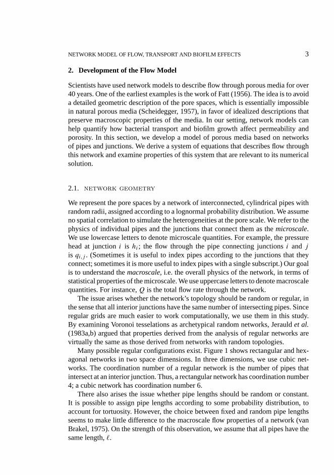
The issue arises whether the network’s topology should be random or regular, inthe sense that all interior junctions have the same number of intersecting pipes. Sinceregular grids are much easier to work computationally, we use them in this study.By examining Voronoi tesselations as archetypical random networks, Jerauldet al.(1983a,b) argued that properties derived from the analysis of regular networks arevirtually the same as those derived from networks with random topologies.

Many possible regular configurations exist. Figure 1 shows rectangular and hex-agonal networks in two space dimensions. In three dimensions, we use cubic net-works. The coordination number of a regular network is the number of pipes thatintersect at an interior junction. Thus, a rectangular network has coordination number4; a cubic network has coordination number 6.

There also arises the issue whether pipe lengths should be random or constant.It is possible to assign pipe lengths according to some probability distribution, toaccount for tortuosity. However, the choice between fixed and random pipe lengthsseems to make little difference to the macroscale flow properties of a network (vanBrakel, 1975). On the strength of this observation, we assume that all pipes have thesame length,.


Figure 1. Square and hexagonal networks used to model two-dimensional porous media.Both networks have size 7× 5.

We designate left-to-right as the overall (horizontal) flow direction, determinedby the macroscopic head gradient. Denote byM, the number of junctions in the flowdirection; letN be the number of junctions in the vertical direction and, in threedimensions, letP be the number of junctions in horizontal direction orthogonal tothe overall flow direction. Thus, the size of a two-dimensional rectangular grid isM × N , and the size of a three-dimensional cubic grid isM × N × P .

2.2. flow physics

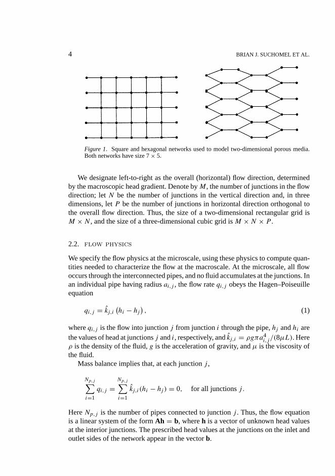
We specify the flow physics at the microscale, using these physics to compute quan-tities needed to characterize the flow at the macroscale. At the microscale, all flowoccurs through the interconnected pipes, and no fluid accumulates at the junctions. Inan individual pipe having radiusai,j , the flow rateqi,j obeys the Hagen–Poiseuilleequation

qi,j = kj,i(hi − hj

), (1)

whereqi,j is the flow into junctionj from junctioni through the pipe,hj andhi arethe values of head at junctionsj andi, respectively, andkj,i = ρgπa4

i,j /(8µL). Hereρ is the density of the fluid,g is the acceleration of gravity, andµ is the viscosity ofthe fluid.

Mass balance implies that, at each junctionj ,

Np,j∑i=1

qi,j =Np,j∑i=1

kj,i(hi − hj ) = 0, for all junctionsj .

HereNp,j is the number of pipes connected to junctionj . Thus, the flow equationis a linear system of the formAh = b, whereh is a vector of unknown head valuesat the interior junctions. The prescribed head values at the junctions on the inlet andoutlet sides of the network appear in the vectorb.


The macroscale volumetric flow rateQ through the grid is the sum of themicroscale flow rates through the outlet side of the grid. Under the hypothesis thatthe macroscale flow obeys Darcy’s law, the permeability of the network is

K = − QL

A 1H,

whereA is the cross-sectional area of the network,L is its length, and1H is the nethead drop between its left and right boundaries. We discuss the Darcy hypothesis inSection 7.

2.3. solving the linear system

We now show that the coefficient matrix,A, for the flow equation is sparse, symmetric,weakly diagonally dominant, irreducible, and positive definite.

First, consider the zero structure ofA. In two dimensions, a square grid has acoordination number of 4, while a hexagonal grid has a coordination number of 3.In three dimensions, a cubic grid has a coordination number of 6. Therefore, thematrix A for a square grid has at most four nonzero off-diagonal elements in a row.The matrix for a hexagonal grid has at most three nonzero off-diagonal elements ina row, and a cubic grid has at most six. Similarly,A has at most four, three, and sixoff-diagonal entries, respectively, in each column.

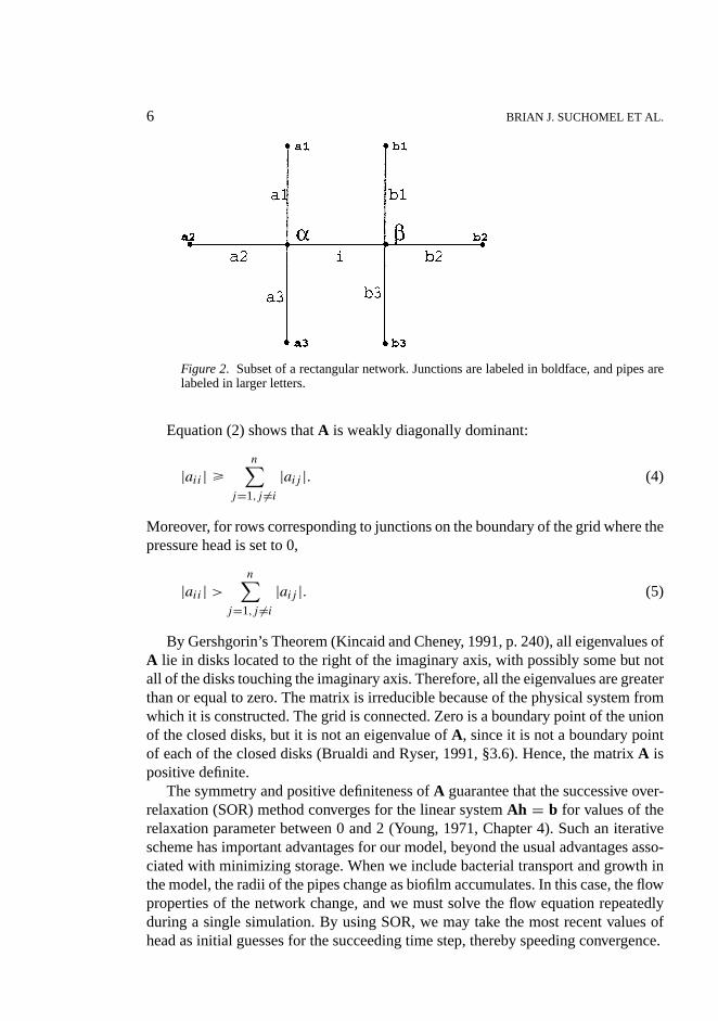
Next, we establish thatA is symmetric. The mass balance furnishes one equationfor each node. Alternatively, we may view each pipe as directly influencing twoequations. In a two-dimensional square grid, consider the pipe connecting junctionsα andβ, with flow coefficientkα,β , as shown in Figure 2. Associated with junctionα is a row inA representing the equation

ka1,α(hα−ha1) + ka2,α(hα − ha2) + ka3,α(hα − ha3) + kα,β(hα − hβ) = 0.

We can rearrange this equation as follows:

(ka2,α + kα,β + ka1,α + ka3,α)hα −− kα,βhβ − ka1,αha1 − ka2,αha2 − ka1,αha1 = 0. (2)

Therefore, the diagonal entries are positive. Also the entryaα,β in the matrixA is−kα,β . Associated with junctionβ we have the equation

(kα,β + kb1,β + kb2,β + kb3,β)hβ −− kα,βhα − kb1,βhb1 − kb2,βhb2 − kb1,βhb1 = 0. (3)

Thus,aβ,α = −kα,β = aα,β whenα andβ are indices of adjacent junctions. Fornonadjacent junctionsα andβ, aα,β = 0 = aβ,α. It follows that the matrixA is realand symmetric and, therefore, all eigenvalues ofA are real. Similar reasoning appliesto hexagonal and cubic networks.


Figure 2. Subset of a rectangular network. Junctions are labeled in boldface, and pipes arelabeled in larger letters.

Equation (2) shows thatA is weakly diagonally dominant:

|aii | >

n∑j=1,j 6=i

|aij |. (4)

Moreover, for rows corresponding to junctions on the boundary of the grid where thepressure head is set to 0,

|aii | >

n∑j=1,j 6=i

|aij |. (5)

By Gershgorin’s Theorem (Kincaid and Cheney, 1991, p. 240), all eigenvalues ofA lie in disks located to the right of the imaginary axis, with possibly some but notall of the disks touching the imaginary axis. Therefore, all the eigenvalues are greaterthan or equal to zero. The matrix is irreducible because of the physical system fromwhich it is constructed. The grid is connected. Zero is a boundary point of the unionof the closed disks, but it is not an eigenvalue ofA, since it is not a boundary pointof each of the closed disks (Brualdi and Ryser, 1991, §3.6). Hence, the matrixA ispositive definite.

The symmetry and positive definiteness ofA guarantee that the successive over-relaxation (SOR) method converges for the linear systemAh = b for values of therelaxation parameter between 0 and 2 (Young, 1971, Chapter 4). Such an iterativescheme has important advantages for our model, beyond the usual advantages asso-ciated with minimizing storage. When we include bacterial transport and growth inthe model, the radii of the pipes change as biofilm accumulates. In this case, the flowproperties of the network change, and we must solve the flow equation repeatedlyduring a single simulation. By using SOR, we may take the most recent values ofhead as initial guesses for the succeeding time step, thereby speeding convergence.


We use a residual criteria for convergence. Define the vectorr by

ri = bi −n∑

j=1

ai,jhj .

We iterate until max{ri} < ε, whereε is some pre-set tolerance. We computer everytenth iteration. The residual at nodei amounts to the sum of volumetric flow ratesout of that node.

3. Development of the Transport Model

Modeling biofilm growth in the network requires solving for the transport of biofilm-forming bacteria through the pipes. Among the earliest work in modeling transport innetworks is that of Simon and Kelsey (1971). They modeled miscible displacement ofone fluid by another by tracking concentration fronts in the pipes, assuming completemixing at the junctions. Sugitaet al. (1995) used a particle-tracking technique inwhich each computational particle represents a given mass of solute.

In contrast, we adopt a Eulerian viewpoint and model concentrations at fixedpoints in the network. More specifically, we use finite differences to model transportin each of the individual pipes. In this section, we describe this transport model indetail.

3.1. transport physics

We model transport within each pipep as a one-dimensional process obeying theequation

∂u

∂t+ vp

∂u

∂x− D

∂2u

∂x2 = 0. (6)

Here,D is the longitudinal (axial) diffusion coefficient,u is concentration, andvp isthe mean velocity through the pipe.

We calculatevp, using the microscopic flow equation, as follows: the heads at thejunctions of the network determine the volumetric flow rates through individual pipesvia Equation (1). We compute the mean fluid velocity through pipep by dividing thevolumetric flow rate by the cross-sectional area of the pipe

vp = qp

πa2p

. (7)

We will discuss the treatment of longitudinal diffusion,D, shortly.

3.2. discretizing the pipes

Equation (6) can be solved exactly but, in general, for bounded spatial domains thesolution involves an infinite series that is expensive to evaluate. Instead, we proposeto use a finite difference approximation as described below.


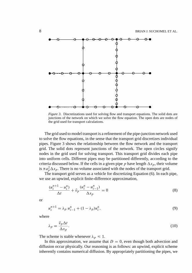
Figure 3. Discretizations used for solving flow and transport equations. The solid dots arejunctions of the network on which we solve the flow equation. The open dots are nodes ofthe grid used for transport calculations.

The grid used to model transport is a refinement of the pipe-junction network usedto solve the flow equations, in the sense that the transport grid discretizes individualpipes. Figure 3 shows the relationship between the flow network and the transportgrid. The solid dots represent junctions of the network. The open circles signifynodes in the grid used for solving transport. This transport grid divides each pipeinto uniform cells. Different pipes may be partitioned differently, according to thecriteria discussed below. If the cells in a given pipep have length1xp, their volumeis πa2

p1xp. There is no volume associated with the nodes of the transport grid.The transport grid serves as a vehicle for discretizing Equation (6). In each pipe,

we use an upwind, explicit finite-difference approximation,

(un+1i − un

i )

1t+ vp

(uni − un

i−1)

1xp= 0 (8)

or

un+1i = λp un

i−1 + (1 − λp)uni , (9)

where

λp = vp1t

1xp. (10)

The scheme is stable wheneverλp < 1.In this approximation, we assume thatD = 0, even though both advection and

diffusion occur physically. Our reasoning is as follows: an upwind, explicit schemeinherently contains numerical diffusion. By appropriately partitioning the pipes, we


can adjust the numerical diffusion to control the effective diffusion in the pipes. Wenow discuss the details of this procedure.

3.3. controlling numerical diffusion

To quantify the numerical diffusion in Equation (8), we examine Taylor expansionsfor each term about a point midway between spatial nodesi − 1 andi and midwaybetween time levelsn andn+1. Substituting these expansions into the scheme yields

(un+1i − un

i )

1t+ vp

(uni − un

i−1)

1xp

= ∂u

∂t

∣∣∣∣n+ 12

i− 12

+ vp∂u

∂x

∣∣∣∣n+ 12

i− 12

+ (1xp − vp1t)

2

∂2u

∂x∂t

∣∣∣∣∣n+ 1

2

i− 12

+ O((1xp + 1t)2).

The first two terms on the right are identical to those in the diffusion-free transportequation. By using the transport equation, we write the mixed derivative in the thirdterm on the right as

−Dnump

∂2u

∂x2

∣∣∣n+ 12

i− 12

,

where

Dnump = vp1xp(1 − λp)

2. (11)

Thus, up toO((1xp+1t)2), the Scheme (8) approximates the diffusion-free transportequation and adds numerical diffusion given by Equation (11).

This analysis allows us to control the numerical diffusion generated in the indi-vidual pipes by adjusting the numbersN1, N2, . . . , NP of cells in each of the pipes,indexed 1, 2, . . . , P , and the common time step1t . To facilitate the discussion, wedefine dimensionless position and time variables

ξ = x

L, τp = vpt

L.

In terms of these variables, the cell length in pipep is1ξp = 1/Np, and the numericaldiffusion there is

Dnump = vpL(1ξp − 1τp)

2(12)

= vpL

2

(1

Np− 1τp

). (13)

Stability requires thatDnump > 0, which implies that

1t <L

vpNp, k = 1, 2, . . . , P . (14)


To impose this condition across the entire network, we choose

1t <L

|vmax|Nmin, (15)

whereNmin is the smallest number of cells allowed in any pipe andvmax is thelargest-magnitude mean velocity occurring among the pipes. This way, if we assignNp = Nmin for any pipe in which|vp| = |vmax|, we haveDnum

k = 0 in that pipe. Tominimize numerical diffusion elsewhere, we divide other pipes into as many cells aspossible, subject to the constraint that

Np <L

vp1t.

In other words, we want

Np <1

1τp< Np + 1. (16)

When the flow through a pipe is very slow, the criterion (16) calls for very largevalues ofNp. To avoid impractical computational expense, we set an upper boundNmax on the number of cells allowed in any pipe. Thus,

Np = min

{⌊1

vp1t

⌋, Nmax

}, (17)

whereb·c denotes the greatest integer function.If we chooseNmax to be the smallest positive integer satisfying

Nmax >

√Nmin(Nmin + 1)2

2, (18)

then the numerical diffusion generated in any pipe obeys the bound

max(Dnump ) <

vmaxL

2(Nmin + 1)2 . (19)

4. Boundary Conditions

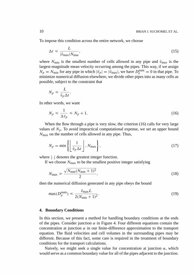
In this section, we present a method for handling boundary conditions at the endsof the pipes. Consider junctionα in Figure 4. Four different equations contain theconcentration at junctionα in our finite-difference approximation to the transportequation. The fluid velocities and cell volumes in the surrounding pipes may bedifferent. Because of this fact, some care is required in the treatment of boundaryconditions for the transport calculations.

Naively, we might seek a single value for concentration at junctionα, whichwould serve as a common boundary value for all of the pipes adjacent to the junction.


Figure 4. The pipes surrounding nodeα. Flow directions in the pipes are indicated by thearrows.

However, a simple example illustrates why this is impossible. In our finite-differencescheme, the concentration at junctionα would have to obey both of the followingequations:

un+1α = λau

na3 + (1 − λa)u

nα

and

un+1α = λbu

nb5 + (1 − λb)u

nα,

whereλa = va1t/1xa andλb = vb1t/1xb. These equations need not give thesame value foruα.

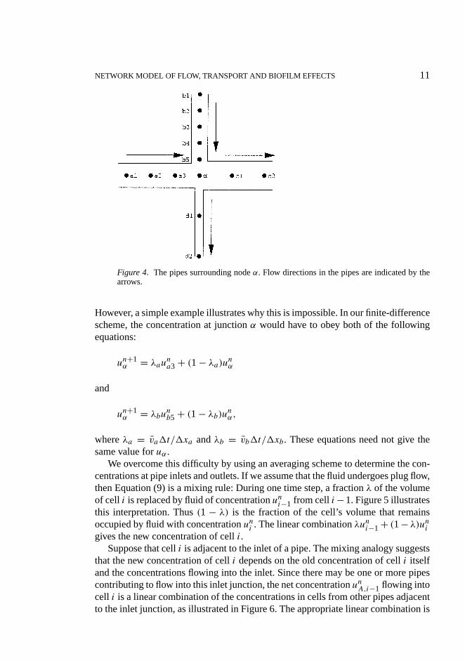
We overcome this difficulty by using an averaging scheme to determine the con-centrations at pipe inlets and outlets. If we assume that the fluid undergoes plug flow,then Equation (9) is a mixing rule: During one time step, a fractionλ of the volumeof cell i is replaced by fluid of concentrationun

i−1 from cell i −1. Figure 5 illustratesthis interpretation. Thus(1 − λ) is the fraction of the cell’s volume that remainsoccupied by fluid with concentrationun

i . The linear combinationλuni−1 + (1− λ)un

i

gives the new concentration of celli.Suppose that celli is adjacent to the inlet of a pipe. The mixing analogy suggests

that the new concentration of celli depends on the old concentration of celli itselfand the concentrations flowing into the inlet. Since there may be one or more pipescontributing to flow into this inlet junction, the net concentrationun

A,i−1 flowing intocell i is a linear combination of the concentrations in cells from other pipes adjacentto the inlet junction, as illustrated in Figure 6. The appropriate linear combination is


Figure 5. Interpretation ofλ as the fraction of the cell that the fluid moves through in onetime step1t .

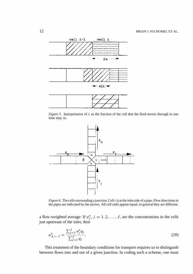
Figure 6. The cells surrounding a junction. Celli is at the inlet side of a pipe. Flow directions inthe pipes are indicated by the arrows. All cell radii appear equal; in general they are different.

a flow-weighted average: Ifunj , j = 1, 2, . . . , J , are the concentrations in the cells

just upstream of the inlet, then

unA,i−1 =

∑Jj=1 un

j qj∑Jj=1 qj

. (20)

This treatment of the boundary conditions for transport requires us to distinguishbetween flows into and out of a given junction. In coding such a scheme, one must


store the indices of the pipes that meet at a each junction, along with the direction ofthe flow from each pipe.

Other authors have proposed models for partial mixing at junctions. Hull andKoslow (1986) investigate streamline routing in 2-D planar, perpendicular junctions.Philip (1988) does a more thorough investigation of the same phenomena. Both setsof authors assume perpendicular junctions with very simple geometries. Naturallyoccuring porous media do not exhibit these characteristics. We have neglected tor-tuosity factors in our pipe lengths and volume at the junctions in our model. We donot presume that pipes enter junctions at right angles. We use a simple flow weight-ed average, which assumes complete mixing, as a reasonable approximation. Ourmodel does allow for there to be either only one pipe entering or one pipe leaving ajunction, in which case, either no mixing is encountered, or complete mixing is theonly possibility.

5. Visualization

In any computational study of scale-up from microscale to macroscale, the issue ofvisualization arises. In our model, flow and transport are essentially one-dimensionalat the microscopic scale, but they may be two- or three-dimensional macroscopically,depending on the type of network used. Displaying all of the pipe radii and flow ratesand the concentrations in all cells at each time level requires animation of a finelydetailed database.

Instead, we adopt a simpler visualization scheme that still captures the macro-scopic behavior of the system. We display mean concentrations at the junctions of thenetwork, calculated in a fashion similar to that used to calculate inlet concentrationsin the transport model. However, for visualization, we use weighted averages basedon static volumes (or, equivalently, cross-sectional areas) of the pipes meeting at ajunction, rather than on flow rates. To illustrate this scheme, consider the junctionshown in Figure 6. Letaα,aβ ,aγ , andai be the radii of the pipes surrounding the nodeand letcα, cβ , cγ , andci be the corresponding concentrations at the midpoints of thecells bordering the node. The static-volume averaging scheme yields the followingconcentration at the node:

cnode= cαa2α + cβa2

β + cγ a2γ + cia

2i

a2α + a2

β + a2γ + a2

i

.

To plot solute concentration as a function of depth in a square network, we cal-culate the average concentration over all junctions in each column. Again, we usestatic-volume averaging: in columnj , the average concentration is

cj =∑N

i=1

(∑α ci,j,αa2

i,j,α

)∑N

i=1

(∑α a2

i,j,α

) .


In this equation,i indexes the row in the network,j indexes the column, and thetriple (i, j, α) indexes the∝th cell bordering on the junction at rowi, columnj . Thiscell has radiusai,j,α.

In three-dimensional networks, we display breakthrough curves by averaging theconcentrations of cells at the outlet side of the network, using flow rates for theweighting. If α, β, . . . are the indices of the cells adjacent to the outlet side ofthe network, with corresponding volumetric flow ratesqα, qβ, . . ., the macroscopiceffluent concentration is

Cout = cαqα + cβqβ + · · ·qα + qβ + · · · .

6. Inclusion of Biofilm Phenomena

Modeling biofilm growth and transport in the network requires keeping track of atleast two species: bacteria and one type of nutrient. We also assume that we havetwo phases present within the pipes: a solution phase and an adsorbed (biofilm)phase. The total volume of a pipe is given at the beginning of a simulation. It isdivided evenly among the cells in the pipe. The solution phase occupies the entirevolume of a cell. The adsorbed phase occupies a portion of the volume of a celldetermined by its concentration and density. Physically, a biofilm is composed mainlyof fluid (Christensen and Characklis, 1990). We consider it, not as a solid, but asa phase occupying a certain volume which may also be occupied by species in thesolution phase. We ignore transport processes between the bulk phase and the biofilm.The biofilm decreases the effective radius of a cell. This decreases the effectiveconductivity of the cell, and hence the conductivity of the pipe.

We treat each cell in the transport grid as a tank reactor connected only to cellsthat are immediately upstream or downstream. Within each cell, species concentra-tions are spatially uniform, and some of a species’ mass may be in the adsorbedphase (biofilm), while the rest is in solution. Mass in solution undergoes transportvia advection, while adsorbed mass undergoes no advection or diffusion. The con-centrations of the species are coupled, since bacteria consume nutrients. In addition,there may be some mass transport of bacteria between phases.

We incorporate adsorption into our model with a novel approach. The thicknessof the biofilm influences the radius of a pipe. Letao be the radius initially assigned toa pipe by the probability distribution. We assume that any concentration of a speciesin the adsorbed phase adheres to the walls of the pipe, decreasing its effective radiusby an amount equal to the thickness of the biofilm. The dissolved species do notaffect the size of a pipe. LetcB be the total adsorbed concentration in a cell, and letρB be the density of the biofilm. The fractioncB/ρB has units of biofilm volume percell volume. The radius at timet is

at = ao

√1 − cB(t)

ρB(t). (21)


The biofilm thickness in the cell is therefore

dB,t = ao − at .

Mass is conserved in all components at each step. In solving the flow equationwe impose a no accumulation condition at each node. We have conservation of massbetween species within each cell. All carbon lost from the nutrient concentration isaccounted for as gains in other concentrations. Mass transfer of bacteria between theadsorbed and solution phases does not affect total mass. Since we assume that thesolution phase occupies the entire cell, there is no loss of fluid.

A biofilm affects the radii of the pipes which, in turn, affect the coefficientsk inthe flow equation. In principle, biofilm-induced changes in pipe radii require us tosolve the flow equations iteratively at each time level, to account for the couplingbetween flow and transport. When biofilm growth is slow enough, the flow propertiesof the network do not change significantly within a time step, and computationallyit may not be necessary to solve the flow equation at every time step. Instead, toreduce computational expense, we assume that the pipe velocities remain unchangedfor several time levels.

When we do compute new flow rates through the grid, we redistribute biofilmconcentrations. We calculate the biofilm concentration of a pipe as the arithmeticmean of the concentrations of the individual cells in the pipe. Then we calculate thenew radii of the pipes using Equation (21) and use these radii to calculatek values.

At the beginning of a simulation all of the pipes have positive radii. As a simulationprogresses and a biofilm grows in the pipes, some of the radii may go to zero. Thematrix becomes singular if all of the pipes meeting at any given node become zero atthe same time. This corresponds to a zero row in the matrix and a zero right-hand side.Any value for pressure head is acceptable at that node, since there will not be any flowinto or out of the node for anyh. We essentially decrease the number of unknowns byone when this happens. Another situation can develop which causes more significantnumerical problems. There will be no solution toAh = b when a whole column ofconnected nodes have zero flow, and our iterative scheme will not converge. Thiscorresponds physically to complete clogging of the medium. Simulation results nolonger make sense after this point.

The discussion presented here describes just the rudiments of biofilm modeling.A complete description of the PDEs and ODEs used in incorporating biofilm effectsinto a network model may be found in a companion paper (Suchomelet al., 1998).That paper also describes reaction and phase change kinetics along with stabilitycriteria and a stable integration scheme.

7. Numerical Results

To verify that the coupled flow-and-transport model produces physically reason-able results, we examine numerical results from several model problems. We assesswhether the flow model produces macroscopic velocities consistent with Darcy’s


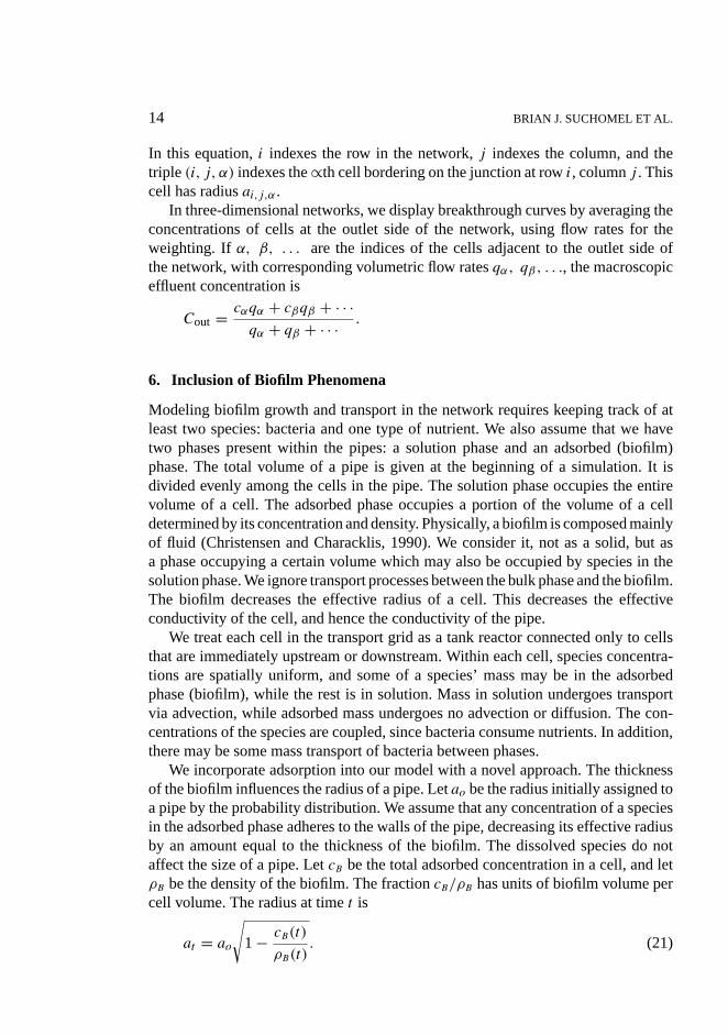
Figure 7. Variability in the ratioQ/1H over suites of 100 realizations of networks withrandomly assigned pipe radii.

law, whether the transport model yields macroscopic plumes that agree with stan-dard models of hydrodynamic dispersion, and whether the coupled model computesplausible results for biofilm growth and transport. In a companion paper (Suchomeletal., 1998) we present more detailed results relating to the scale-up of biofilm growthand transport.

We begin with the flow calculations. Here the question is whether or not it is rea-sonable to calculate a macroscopic permeability by averaging the results of the micro-scopic model. Many naturally occurring porous media have irregular pore spaces withsome degree of randomness in their configurations. We expect some small variationsin the permeabilities in different samples of these substances. By analogy, within anysuite of networks having pipe radii assigned from a fixed probability distribution, weexpect some variations in the apparent macroscale permeability.

Figure 7 shows how the ratioQ/1H varies within suites of one hundred 20× 20networks, each suite having pipe radii assigned from a lognormal distribution havingmeanµ = 1. The figure shows histograms ofQ/1H for four different choices ofstandard deviation in the lognormal distribution. We conclude from this figure thatapparent macroscale permeabilities tend to cluster around a central, representativevalue, especially at smaller values of standard deviation. This result is expected sincesmaller standard deviations represent more homogeneous media. We useσ = 0.6for most of our calculations, since it represents an average porous medium and isalso near the middle of the range of values used by other authors which go fromσ = 0.02 to 1.2. Sugitaet al. (1995) claim thatσ = 0.2 to 0.3 is representative of


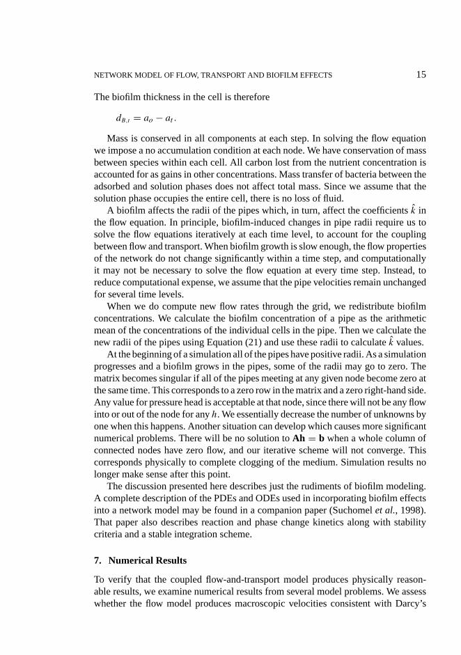
Figure 8. Dependence of flow to head drop ratio on width and length of a grid. All valuesplotted represent the mean of 100 realizations. The mean pore size is 1 in all realizations.Standard deviations of the log-normal distributions are shown by the curves.

an actual homogeneous porous medium and Imdakm and Sahimi (1991) claim thatσ = 2

3 closely approximates experimentally-determined pore size distributions ofOttawa sandpack.

Of more direct interest is the question whetherQ/1H varies linearly with thelength of the medium, i.e., whether Darcy’s law is a valid hypothesis for the macro-scopic flow. Figure 8 suggests that Darcy’s hypothesis is valid and that, for a givenlength, the medium’s permeability decreases as the standard deviation in pipe diam-eters increases.

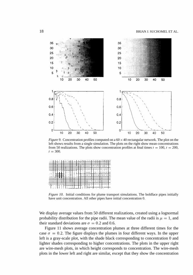
Next, we examine the model’s results for macroscopic, biofilm-free transport.Figure 9 shows concentration fronts entering an initially solute-free network, com-puted using a two-dimensional, rectangular network. Here, the macroscopic flowdirection is from left to right. Fort > 0, all of the fluid entering the grid has unitconcentration. The top two plots show concentration fronts at timet = 300. Thebottom two plots show mean concentration as a function of depth. The plots on theleft show results for a single realization, while the plots on the right show mean con-centrations computed from 50 realizations of the network, each having a differentassignment of pipe radii using a lognormal distribution, withµ = 1 andσ = 0.6.

As the figure shows, solute distributions in a single realization typically exhibit fin-gering, reflecting the fact that solute advects preferentially through the larger pipes.Averaging several realizations smooths out the fingers, yielding fronts that exhibitthe diffusion-like spreading associated with stochastic solute transport.

In addition to concentration fronts, we examine the transport of concentrationplumes by assigning nonzero initial concentration in some pipes while leaving otherpipes solute-free. Figure 10 shows the pipes in a 30×20 rectangular network that haveunit initial concentration. All other pipes in the network have initial concentration 0.


Figure 9. Concentration profiles computed on a 60×40 rectangular network. The plot on theleft shows results from a single simulation. The plots on the right show mean concentrationsfrom 50 realizations. The plots show concentration profiles at final timest = 100,t = 200,t = 300.

Figure 10. Initial conditions for plume transport simulations. The boldface pipes initiallyhave unit concentration. All other pipes have initial concentration 0.

We display average values from 50 different realizations, created using a lognormalprobability distribution for the pipe radii. The mean value of the radii isµ = 1, andtheir standard deviations areσ = 0.2 and 0.6.

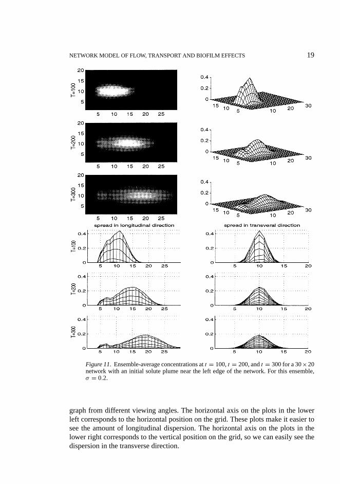
Figure 11 shows average concentration plumes at three different times for thecaseσ = 0.2. The figure displays the plumes in four different ways. In the upperleft is a gray-scale plot, with the shade black corresponding to concentration 0 andlighter shades corresponding to higher concentrations. The plots in the upper rightare wire-mesh plots, in which height corresponds to concentration. The wire-meshplots in the lower left and right are similar, except that they show the concentration


Figure 11. Ensemble-average concentrations att = 100,t = 200, andt = 300 for a 30×20network with an initial solute plume near the left edge of the network. For this ensemble,σ = 0.2.

graph from different viewing angles. The horizontal axis on the plots in the lowerleft corresponds to the horizontal position on the grid. These plots make it easier tosee the amount of longitudinal dispersion. The horizontal axis on the plots in thelower right corresponds to the vertical position on the grid, so we can easily see thedispersion in the transverse direction.


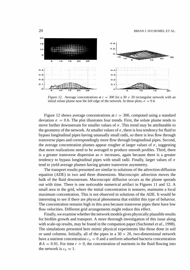
Figure 12. Average concentrations att = 300 for a 30× 20 rectangular network with aninitial solute plume near the left edge of the network. In these plots,σ = 0.6.

Figure 12 shows average concentrations att = 300, computed using a standarddeviationσ = 0.6. The plot illustrates four trends. First, the solute plume tends tomove further downstream for smaller values ofσ . This trend may be attributable tothe geometry of the network. At smaller values ofσ , there is less tendency for fluid tobypass longitudinal pipes having unusually small radii, so there is less flow throughtransverse pipes and correspondingly more flow through longitudinal pipes. Second,the average concentration plumes appear rougher at larger values ofσ , suggestingthat more realizations need to be averaged to produce smooth profiles. Third, thereis a greater transverse dispersion asσ increases, again because there is a greatertendency to bypass longitudinal pipes with small radii. Finally, larger values ofσ

tend to yield average plumes having greater transverse asymmetry.The transport results presented are similar to solutions of the advection-diffusion

equation (ADE) in two and three dimensions. Macroscopic advection moves thebulk of the fluid downstream. Macroscopic diffusion occurs as the plume spreadsout with time. There is one noticeable numerical artifact in Figures 11 and 12. Asmall area in the grid, where the initial concentration is nonzero, maintains a localmaximum concentration. This is not observed in solutions of the ADE. It would beinteresting to see if there are physical phenomena that exhibit this type of behavior.The concentration remains high in this area because transverse pipes there have lowflow velocities. Different grid arrangements might reduce this effect.

Finally, we examine whether the network models gives physically plausible resultsfor biofilm growth and transport. A more thorough investigation of this issue alongwith scale-up results, may be found in the companion paper (Suchomelet al., 1998).The simulations presented here mimic physical experiments like those done in soilor sand columns. Initially, all of the pipes in a 30× 20, two-dimensional networkhave a nutrient concentrationcn = 0 and a uniform adsorbed bacteria concentrationBA = 0.01. For timet > 0, the concentration of nutrients in the fluid flowing intothe network iscn = 1.


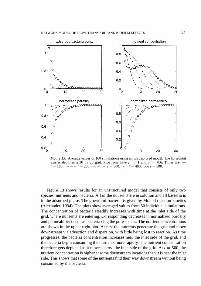
Figure 13. Average values of 100 simulations using an unstructured model. The horizontalaxis is depth in a 30 by 20 grid. Pipe radii haveµ = 1 andσ = 0.6. Times are: —t = 100; − − − t = 200; −. − . − t = 300; · · · t = 400; ooot = 500.

Figure 13 shows results for an unstructured model that consists of only twospecies: nutrients and bacteria. All of the nutrients are in solution and all bacteria isin the adsorbed phase. The growth of bacteria is given by Monod reaction kinetics(Alexander, 1994). The plots show averaged values from 50 individual simulations.The concentration of bacteria steadily increases with time at the inlet side of thegrid, where nutrients are entering. Corresponding decreases in normalized porosityand permeability occur as bacteria clog the pore spaces. The nutrient concentrationsare shown in the upper right plot. At first the nutrients penetrate the grid and movedownstream via advection and dispersion, with little being lost to reaction. As timeprogresses, the bacteria concentration increases near the inlet side of the grid, andthe bacteria begin consuming the nutrients more rapidly. The nutrient concentrationtherefore gets depleted as it moves across the inlet side of the grid. Att = 500, thenutrient concentration is higher at some downstream locations than it is near the inletside. This shows that some of the nutrients find their way downstream without beingconsumed by the bacteria.


8. Conclusions

Network models of porous media have been in use for over 40 years. In this paper,we create a new type of network simulator specifically for modeling biofilm growthand transport. In this pipe-and-junction model, the equations for the fluid flow yield acoefficient matrix that is symmetric and positive definite and, hence, the system maybe solved using an iterative SOR technique. We develop a new method for modelingtransport in the network. This method employs an upwind, explicit finite-differencescheme within each pipe, together with a partitioning technique that enables us tobound the numerical diffusion generated in each pipe. A simple adsorption modelaccounts for bacteria and nutrients and their interactions. We compute macroscopicproperties of the flow such as porosity and permeability and their dependence on theamount of biomass. Such a model is useful in the scale-up of microscopic dynamicsto macroscopic descriptions needed in continuum-level models of biofilms in porousmedia. A sequel (Suchomelet al., 1998) to this paper describes this application.

References

Alexander, M.: 1994,Biodegradation and Bioremediation, Academic Press, New York.Brualdi, B. A. and Ryser, H. J.: 1991,Combinatorial Matrix Theory, Cambridge University Press.Christensen, B. E. and Characklis, W. G.: 1990, Physical and Chemical Properties of Biofilms,

In: W. G. Characklis and K. C. Marshall (eds),Biofilms, Wiley-Interscience, New York, pp.93–130.

Hull, L. C. and Koslow, K. N.: 1986, Streamline routing through fracture junctions,Water Resour.Res.22(12), 1731–1734.

Imdakm, A. O. and Sahimi, M.: 1991, Computer simulation of particle transport processes in flowthrough porous media,Chem. Eng. Sci.46(8), 1977–1993.

Jerauld, G. R., Hatfield, J. C., Scriven, L. E. and Davis, H. T.: 1984a, Percolation and conductionon Voronoi and triangular networks: a case study in topological disorder,J. Phys. C: Solid StatePhys.17, 1519–1529.

Jerauld, G. R., Scriven, L. E. and Davis, H. T.: 1984b, Percolation and conduction on the 3D Voronoiand regular networks: a second case study in topological disorder,J. Phys. C: Solid State Phys.17, 3429–3439.

Kincaid, D. and Cheney, W.: 1991,Numerical Analysis, Brooks/Cole Publ. Co., Pacific Grove, Ca.,p. 690.

Koplik, J.: 1982, Creeping flow in two-dimensional networks,J. Fluid Mech.119, 219–247.Koplik, J. and Lasseter, T.: 1982, Two-phase flow in random network models of porous media,

Paper presented at 57th Annual Fall Technical Conference and Exhibition of the Society ofPetroleum Engineers of AIME.

Lindqvist, R., Cho, J. S. and Enfield, C. G.: 1994, A kinetic model for cell density dependentbacterial transport in porous media,Water Resour. Res.30(12), 3291–3299.

Philip, J. R.: 1988 The fluid mechanics of fracture and other junctions,Water Resour. Res.24(2),239–246.

Rege, S. and Fogler, H.: 1987, Network model for straining dominated particle entrapment in porousmedia,Chem. Eng. Sci.42(7), 1553–1564.

Scheidegger, A. E.: 1957,The Physics of Flow Through Porous Media, University of Toronto Press.Simon, R. and Kelsey, F. J.: 1971, The use of capillary tube networks in reservoir performance

studies: I. equal-viscosity miscible displacements,Soc. Petrol. Eng. J.11, 99–112.Simon, R. and Kelsey, F. J.: 1971, The use of capillary tube networks in reservoir performance

studies: II. effect of heterogeneity and mobility on miscible displacement efficiency,Soc. Petrol.Eng. J.12, 345–351.


Suchomel, B. J., Chen, B. M. and Allen, M. B.: 1998, Macro-scale properties in porous media froma network model,Transport in Porous Media(to appear).

Sugita, F., Gillham, R. W. and Mase, C.: 1995, Pore scale variation in retardation factor as a causeof nonideal breakthrough curves: 2. Pore network analysis,Water Resour. Res.31(1), 113–119.

Tan, Y., Gannon, J. T., Baveye, R. and Alexander, M.: 1994, Transport of bacteria in an aquifersand: experiments and model simulations,Water Resour. Res.30(12), 3243–3252.

Taylor, S. W. and Jaffe, P. R.: 1990a, Biofilm Growth and the related changes in the physicalproperties of a porous medium 1. Experimental investigation,Water Resour. Res.26(9), 2153–2159.

Taylor, S. W., Milly, P. C. D. and Jaffe, P. R.: 1990b, Biofilm growth and the related changes in thephysical properties of a porous medium 2. Permeability,Water Resour. Res.26(9), 2161–2169.

Taylor, S. W. and Jaffe, P. R.: 1990c, Biofilm growth and the related changes in the physicalproperties of a porous medium 3. Dispersivity and model verification,Water Resour. Res.26(9),2171–2180.

van Brakel, J.: 1975, Pore space models for transport phenomena in porous media, review andevaluation with special emphasis on capillary liquid transport,Powder Technol.11, 205–236.

Vandevivere, P. and Baveye, P.: 1992, Effect of bacterial extracellular polymers on the saturatedhydraulic conductivity of sand columns,Appl. Environ. Microbiol.58(5), 1690–1698.

Young, D. M.: 1971,Iterative Solution of Large Linear Systems, Academic Press, New York, p. 570.

network model of flow, transport and biofilm effects in porous media

Documents