necesitate contraunda lege3 newton

Global Scaling Theory Compendium Version 1.2

21.12.2007

Global Scaling TheoryCompendium

Institute for Space Energy Research Ltd. in memoriam Leonard Euler, Munich, Germany

A Natural Phenomenon

Scaling means logarithmic scale-invariance. Scaling is a basic quality of fractal structures andprocesses. The Global Scaling Theory explains why structures and processes of nature are fractaland the cause of logarithmic scale-invariance.

Historical Excursion

Scaling in Physics

In 1967 / 68 Physicists, Richard P. Feyman and James Bjorken discovered the phenomenon ofLogarithmic Scale-Invariance (Scaling) in high-energy physics, exactly, dependent on rest mass,frequency distributions of Baryon resonances.Bjorken J. D. Phys. Rev. D179 (1969) 1547

In 1967 russian Physicist, Simon E. Shnoll discovered process-independent Scaling in the finestructure of histograms of physical and chemical processes, for example, in radioactiv decay and inthermic noise.Shnoll S. E., Oscillatory processes in biological and chemical systems, Moscow, Nauka, 1967Shnoll S. E., Kolombet V. A., Pozharski E. V., Zenchenko T. A., Zvereva I. M., Konradov A. A.,Realization of discrete states during fluctuations in macroscopic processes, Physics Uspekhi 41(10) 1025 - 1035 (1998)

In 1982 – 84, Hartmut Müller discovered Scaling further in the frequency distributions ofelementary particles, nuclei and atoms dependent on their masses, and in the distributions ofasteroids, moons, planets and stars dependent on their orbital factors, sizes and masses.Müller H., Global Scaling // Munich, 2001-2006

Scaling in Biology

In 1981, Leonid L. Chislenko published his work on Logarithmic Scale-Invariance in the frequencydistribution of biological species, dependent on body size and weight. By introducing a logarithmicscale for biologically significant parameters, such as mean body weight and size, Chislenko wasable to prove that sections of increased specie representation repeat themselves in equal intervals(ca. 0.5 Units of the Log based 10 Scale).Chislenko L. L., The structure of the fauna and flora in connection with the sizes of the organisms,Moskow University Press, 1981.

In 1984, Knut Schmidt-Nielsen was able to prove Logarithmic Scale-Invariance in the synthesis oforganisms and in metabolic processes.Schmidt-Nielsen K., Scaling. Why is the animal size so important? Cambridge University Press,1984.


21.12.2007

In 1981, Alexey Zhirmunsky and Viktor Kuzmin discovered process-independent logarithmic scaleinvariance in the development stages in Embryo-, Morpho- and Ontogenesis and in geologicalhistory .Zhirmunsky A. V., Kuzmin V. I., Critical scaling levels in the development of biological systems,Moskow, Nauka, 1982

Scaling in Neurophysiology

We live in a logarithmic world. All of our senses perceive the logarithm of a signal, not the linearintensity of the signal itself. That is why we measure sound volume in decibels, and consequentlyin logarithmic units.

Sounds whose frequencies differentiate themselves by double, quadruple or eight-times, weperceive as a, a’ or a’’, the same sound. This property of our sense of hearing makes it possible forus to differentiate harmony from disharmony. The harmonic sound sequence 1/2 (Octave), 2/3(Fifth), 3/4 (Fourth), 4/5 (Major Third), and so forth is logarithmic, hyperbolic scale-invariant.

Our sense of touch is also calibrated logarithmically. Assuming that one holds in the left hand 100grams and in the right hand 200 grams; if one then adds 10 grams to the left hand, then 20 gramsmust be added to the right hand in order to sense the same weight increase. This fact is known inSensing Physiology as the Weber-Fechner Law (Ernst Heinrich Weber, 1795 – 1878, GustavTheodor Fechner, 1801 – 1887): The strength of a sensory impression is proportional to thelogarithm of strength of the stimulus.

The Weber-Fechner law also touches on our senses of smell and sight. The retina records only thelogarithm, not the number of impinging photons. That is why we can see not only in sunlight butalso at night. Whereas, the number of impinging photons varies by billionths, the logarithm variesonly by twentieths. (Ln 1000,000,000 ≈ 20.72)

Our vision is logarithmically calibrated not only in regards our perception of the intensity of light,but also relative to the lights wave length which we perceive as colors.

Our ability to judge lineal distances is based on the possibility of comparison of sizes and thedetermination of relative measurement scales. The linear perspective assumes a constant sizeproportion that is defined by size enlargement or reduction factor. This factor is multiplied severaltimes with itself in the perspective. From this an exponential function is defined which argument isa logarithm.

The function of our sense organs is concerned with acoustic or electromagnetic wave processes.The logarithmic scale-invariant perception of the world is a consequence of the logarithmic scale-invariant, construction of the world.

Scaling in Mathematics

All natural numbers 1, 2, 3, 4, 5 ... can be constructed from prime numbers. Prime numbers arenatural numbers that are only divisible by the number 1 and themselves without leaving aremainder; accordingly, the numbers 2, 3, 5, 7, 11, 13, 17, 19, 23, 29, 31 … are quasi elementaryparts of the real number continuum. The distribution of the prime numbers among the naturalnumbers is irregular to such an extent that formula for this distribution cannot be defined. Ofcourse, prime numbers become found more seldom the further one moves along the number line.Already in 1795, Carl Friedrich Gauß noticed this. He discovered that the set p1(n) of prime


21.12.2007

numbers up to the number n could be calculated approximate according to the formula p1(n) = n / lnn. The larger the value of n, the more precisely is this law fulfilled; and means that the distributionof the set of prime numbers among the natural numbers is scale-invariant.

Non-prime numbers can clearly be represented as products of prime numbers. One could also saythat non-prime numbers are prime-number clusters. This means that non-prime numbers arecomposed from several prime numbers. In this interpretation, one can derive the prime-factordensity distribution on the number line.

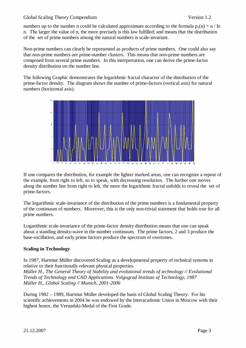
The following Graphic demonstrates the logarithmic fractal character of the distribution of theprime-factor density. The diagram shows the number of prime-factors (vertical axis) for naturalnumbers (horizontal axis).

If one compares the distribution, for example the lighter marked areas, one can recognize a repeat ofthe example, from right to left, so to speak, with decreasing resolution. The further one movesalong the number line from right to left, the more the logarithmic fractal unfolds to reveal the set ofprime-factors.

The logarithmic scale-invariance of the distribution of the prime numbers is a fundamental propertyof the continuum of numbers. Moreover, this is the only non-trivial statement that holds true for allprime numbers.

Logarithmic scale-invariance of the prime-factor density distribution means that one can speakabout a standing density-wave in the number continuum. The prime factors, 2 and 3 produce thebase-oscillation, and early prime factors produce the spectrum of overtones.

Scaling in Technology

In 1987, Hartmut Müller discovered Scaling as a developmental property of technical systems inrelative to their functionally relevant physical properties.Müller H., The General Theory of Stability and evolutional trends of technology // EvolutionalTrends of Technology and CAD Applications. Volgograd Institute of Technology, 1987Müller H., Global Scaling // Munich, 2001-2006

During 1982 – 1989, Hartmut Müller developed the basis of Global Scaling Theory. For hisscientific achievements in 2004 he was endowed by the Interacademic Union in Moscow with theirhighest honor, the Vernadski-Medal of the First Grade.


21.12.2007

From the Model to the Theory

Oscillations are the most energetically efficient kind of movement. For this reason, all matter, notonly each atom, but also the planetary system and our galaxy, oscillate and light is an unfoldingoscillation and, naturally, the cells and organs of our bodies also oscillate.

Based on their energy efficiency, oscillatory processes determine the organization of matter at alllevels – from atoms to galaxies.

In his most meaningful work, “World Harmonic”, Johannes Kepler established the bases forharmonic research. Building on the ancient musical ‘World Harmony’ of the Pythagoreans, Keplerdeveloped a cosmology of harmonics.

Global Scaling research continues this tradition.

The Melody of Creation

Scaling arises very simply – as a consequence of-natural oscillation processes. Natural -oscillations are oscillations of matter that already exist at very low energy levels.

To differentiate from simulated-oscillations, Natural-oscillations therefore occur at the lowestpossible energy level. They, therefore lose little energy, and likewise fulfill the Law of theConservation of Energy.

The energy of an oscillation is dependent on its amplitude as well as on its frequency (events pertime unit).

Consequently, the following is valid for Natural-oscillations: The higher the frequency, the less theamplitude. For Natural-oscillations, the product of frequency and wave length as well as theproduct of frequency and amplitude are conserved. They limit the speed of propagation ofoscillations in mediums, or the speed of deflection.

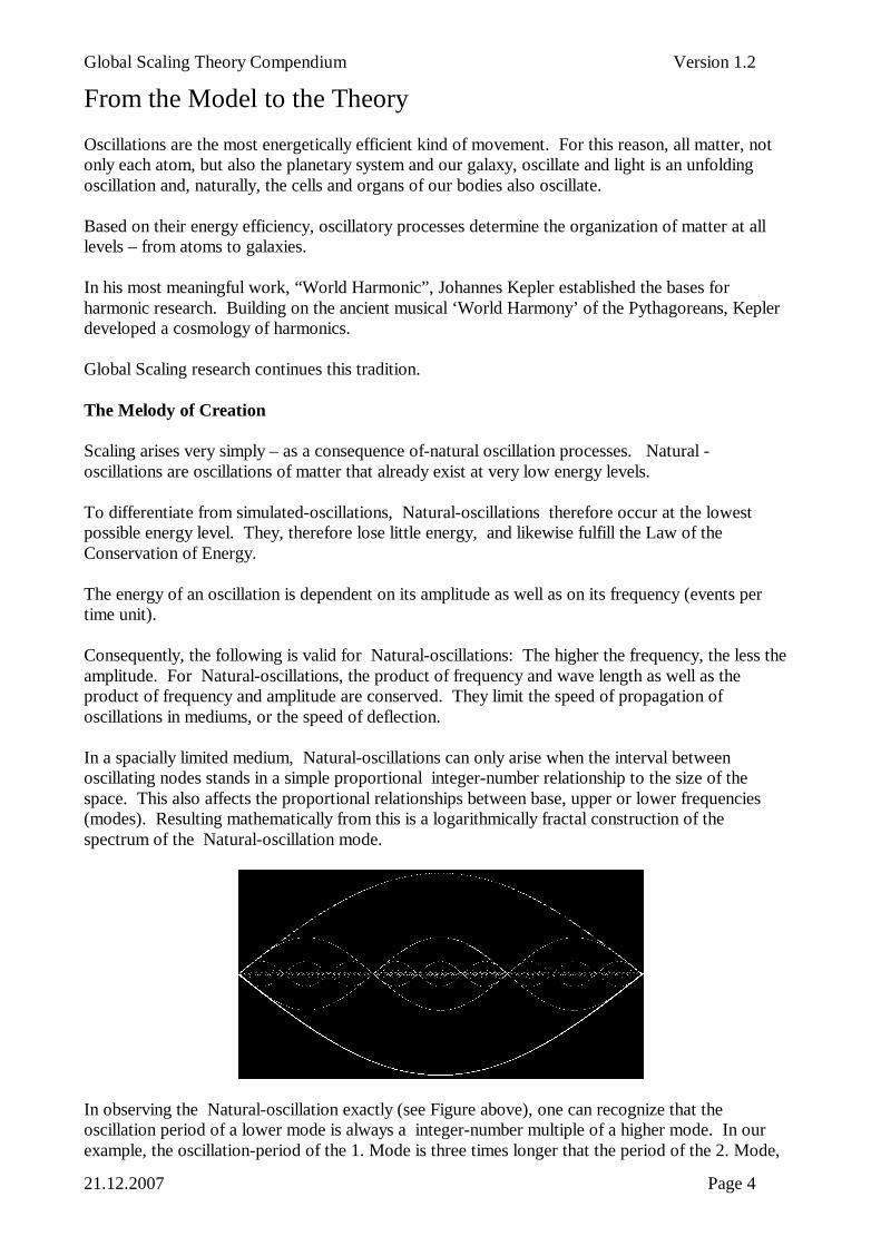
In a spacially limited medium, Natural-oscillations can only arise when the interval betweenoscillating nodes stands in a simple proportional integer-number relationship to the size of thespace. This also affects the proportional relationships between base, upper or lower frequencies(modes). Resulting mathematically from this is a logarithmically fractal construction of thespectrum of the Natural-oscillation mode.

In observing the Natural-oscillation exactly (see Figure above), one can recognize that theoscillation period of a lower mode is always a integer-number multiple of a higher mode. In ourexample, the oscillation-period of the 1. Mode is three times longer that the period of the 2. Mode,


21.12.2007

nine times longer than the period of the 3. Mode and 27 times longer that the period of the 4. Mode.From this follows the logarithmic, fractal, construction of the (repeating itself in all scales)oscillation representation. In this connection, one speaks of scale-invariance (Scaling). In natureScaling is distributed widely – from the elementary particles to the galaxies. It is in this connectionthat one speaks of Global Scaling.

Natural-oscillations of matter produce logarithmic, fractal spectrums of the frequencies, wave-lengths, amplitudes and a logarithmic, fractal network of oscillating-nodes in space.

In physical mediums, base-tones, upper- or undertones are produced simultaneously, and in thisthere arise consonances and dissonances. Not only our hearing can distinguish consonance fromdissonance; this capability extends to all matter, and has to do with the energy expenditurenecessary to produce an overtone. A musical ‘Fifth’ arises most easily (the least expense of energyper oscillation period), because merely a frequency doubling and trebling is necessary in order toproduce an overtone in interval of 3/2 of the base frequency. Somewhat more energy is necessaryto produce a musical ‘Fourth’, 4/3, while this additionally requires a quadrupling of the basefrequency; and even more energy is necessary for the production of the larger musical ‘third’, 6/5,of the same amplitude, and so forth.

The musical intervals accordingly play an energetic, key-role in the spectrum of the Natural-oscillation-modes. In fact, this spectrum is constructed like the spectrum of a melody.

Natural Oscillations of matter are probably the most important structure-forming factor in theUniverse. For this reason one finds fractal proportions everywhere in nature. The logarithmic,fractal distribution of matter in the universe is a consequence of Natural Oscillation processes incosmic, space and time measurement scales. In this connection, one speaks of the “Melody ofCreation.”

Logarithmic periodic structural Change

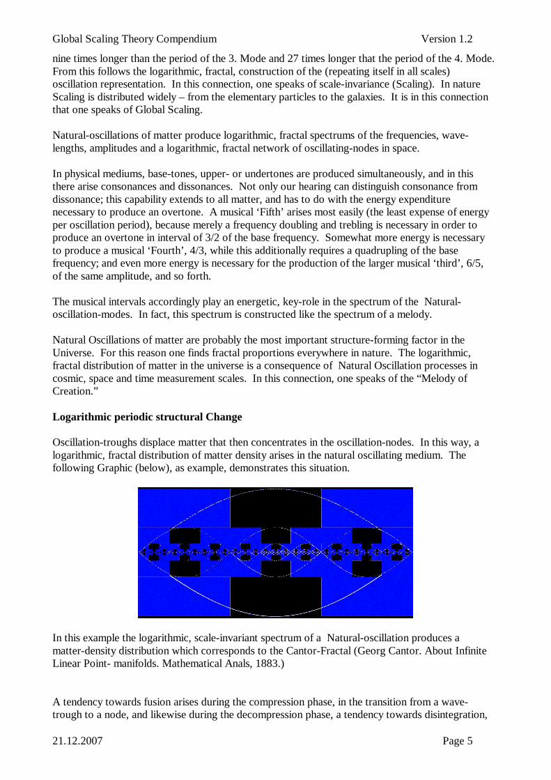
Oscillation-troughs displace matter that then concentrates in the oscillation-nodes. In this way, alogarithmic, fractal distribution of matter density arises in the natural oscillating medium. Thefollowing Graphic (below), as example, demonstrates this situation.

In this example the logarithmic, scale-invariant spectrum of a Natural-oscillation produces amatter-density distribution which corresponds to the Cantor-Fractal (Georg Cantor. About InfiniteLinear Point- manifolds. Mathematical Anals, 1883.)

A tendency towards fusion arises during the compression phase, in the transition from a wave-trough to a node, and likewise during the decompression phase, a tendency towards disintegration,


21.12.2007

in the transition from a node to wave-trough. This change from compression to decompressioncauses a logarithmic, periodic structural change in the oscillating medium; and areas of compressionand decompression arise in a logarithmic, fractal pattern.

A logarithmic-periodic structural change can be observed in all scales of measurement of theuniverse – from atoms to galaxies.

Determined by global logarithmic-periodic compression and decompression change, essentialstructural signposts in the universe repeat themselves unobserved, that it is a question of variousscales of measurement.

Compressed atomic nuclei with a density in the range of 1014 g/cm3 form larger decompressedatoms whose densities, for example for metals this lies between 0.5 and 20 g/cm3. Small moleculesare, as a rule, more compressed than large molecules. Compressed cell nuclei (and other cellorganelles) form relatively decompressed cells. Organisms form (relatively decompressed)populations. Heavenly bodies (moons, planets and stars) form decompressed planetary systems.Compressed star-clusters are, in large measure, detached which again forming relativelycompressed galaxy-clusters.

We have the good fortune that galaxy-clusters belong among the compressed structures in theuniverse. Due to this circumstance, we can be thankful that we know about the existence of othergalaxies. If the matter in the universe were not logarithmic, scale-invariant, but linearly distributed,the distances between galaxies would be proportionally; exactly so large as the distance between thestars in our galaxy, and we would have no chance to ever learn anything of the existence of anothergalaxy. Consequently, Scaling is a global phenomenon, so to speak, the creation plan of theuniverse.

Continued Fraction as Word Formula

In his works “About Continued Fractions” (1737) and “About the Oscillations of a String” (1748),Leonard Euler formulated problems whose solutions would keep the field of mathematics busy for200 years. Euler investigated the Fundamental-oscillations of an elastic, mass-less string of pearls.In connection with this task, d’Alembert developed his method of integration for a system of lineardifferential equations. Daniel Bernoulli asserted his known statement that the solution of theproblem of the free-oscillating string can be represented as trigonometric sequence, somethingwhich started a discussion between Euler, d’Alembert and Bernoulli lasting a decade. Later,Lagrange showed more correctly how one arrives at the solution of the problem of oscillations of astring-of-pearls and the solution of the problem of a homogenous string. The problem-solution wasfirst completely solved by Fourier in 1822.

Almost insurmountable problems arose in the meantime with pearls of various mass and irregulardistribution. This task led to functions with gaps (or voids). After a letter from Charles Hermite,May 20, 1893, who additionally added, “Reject in nervous horror the lamentable annoyance of thefunctions without derivative”; T. Stieltjes investigated functions with discontinuities and found anintegration method for these functions which led to ‘Continued-fractions.’

Meanwhile, Euler already recognized that complex, oscillating systems can contain such solutions(integral) that themselves are not overall differentiateable, and left behind to the futuremathematical world an analytical “Monster” – that is, the non-analytic functions (this term waschosen by Euler himself). Non-analytic functions provided ample and profuse study up to the 20th

century, after the identity crises in mathematics, appeared to be conquered.


21.12.2007

The crises began, and lasted until about 1925, when Emil Heinrich Bois Reymond, in 1875,reported for the first time about a Wierstrass constructed continuous, but non-differentiablefunction. The main players were Cantor, Peano, Lebesgue and Hausdorff; and as a result, a newbranch of mathematics was born – Fractal Geometry.

Fractal comes from the Latin 'fractus' and means “broken-up-in-pieces” and “irregular.” Fractalsare consequently distinct, fragmentary, tricky mathematical objects. Mathematics in the 19th

Century considered these objects as exceptions and from there, tried to derive fractal-objects fromregular, continuous and smooth structures.

The theory of fractal groups made possible in-depth investigations in “non-analytic”, manifold,granular or fragmentary forms. It immediately it becomes apparent that fractal structures are by nomeans so infrequently encountered in the world. More fractal objects are discovered in nature thanever suspected. Moreover, it suddenly seemed as if the entire natural universe were fractal.

Especially, works of Mandelbrot finally advanced the geometry to the position where fractal objectscould be mathematically correctly described: fragmented crystal-lattices, ‘Brownian Motion’ of gasmolecules, complex, giant polymer-molecules, irregular star-clusters, cirrus-clouds, the ‘Rings-of-Saturn,’ the distribution of moon-craters, turbulences in fluids, bizarre coast-lines, snake-like river-streams, faults in mountain-chains, development branches of the most varied kinds of plants,surface areas of islands and lakes, mineral-formations, geological sediments, the distribution inspace of raw-material-occurrences, and, and, and……

A deciding factor in the accurate treatment of fractal objects was the introduction of real and alsoirrational dimensions, in contrast with the whole-number dimensions of Euclidean Geometry. Let’sconsider an example: In Euclidean Geometry, a disappearing, small grain-of-sand has dimension 0.A line – dimension 1. But which dimension does sequence of grains-of-sand arranged one after theother? The Euclidean point of view only knows boundary conditions: Either one proceeds on awide path – until one cannot recognize anymore grains-of-sand and then assigns to this object thedimension 1, or one recognizes the grains-of-sand as objects of dimension 0. and while it is usuallyknown that 0=0=…+0 = 0, the grains-of-sand, are likewise assigned dimension 0. That through thisthe essential is lost is obvious.

The first step of an in-depth analysis of this situation was undertaken by Cantor in his letter of June20th, 1877 to Dedekind, the next was followed by Peano in 1890. The mathematicians recognizedthat an accurate understanding of fractal structures could not be reached when one defines‘dimensions’ as a number of coordinates. Therefore, in 1919 Hausdorff defined a new conception ofdimension. The fractal (broken) dimension D completed the topological (whole-number) dimensionthrough logarithmic values. The fractal dimension of a grain-of-sand sequence of N grains-of-sandof the relative (In comparison to the total length of the sequence) size 1/k, where D = log(N) /log(k). Assuming a sequence of 100 grains-of-sand is 100 mm in length and the size of a grain-of-sand 1 mm. Then D = log (100) / log (100) = 1. However, if the sequence only consists of 50grains-of-sand, then D = log (50) / log (100) = 0.849485. The fractal dimension D is, accordingly, ameasure for the fragmentary nature of an object. The larger the gaps, the further D is from integernumber values.

The application of the Hausdorff-Dimension in geometry now makes it possible to deal with notonly completely irregular real mathematical objects, but at the same time provides the formula forthe creation of home-made fractal creations. The creation of various Mandelbrot- und Julia-groupsusing the computer gave rise to a popular mathematical sport. The Mandelbrot-group is still todaythe object of non-resolved theoretical investigations. However, it is important that these through


21.12.2007

mathematics that their connections become visible, and are being investigated in the most varied ofspecialist fields.

Nevertheless, the fractal ‘Grain-of-sand’ sequence strongly reminds of Euler’s ‘String-of-Pearls.’Both of these objects are fractal. In 1950, the Leningrad mathematicians, F. R. Gantmacher and M.G. Krein regarded the line-of-deflection of an oscillating string of pearls as a broken line. Thisinitial step even enabled them a fractal view of the problem, without which they were unaware(Mandelbrots Classic “Fractal Objects”, appeared in 1975 and was his first works of which 50 werein the field of Linguistics). They first brought the Fractal visibly into the situation, and tocompletely solve (and also for the most general case) the 200 year old Euler Problem of theoscillating “Sting-of-Pearls” for variable masses and irregular Distribution.

In their work, “Oscillation-matrices, Oscillation-nuclei, and Small Oscillations of MechanicalSystems” (Leningrad, 1950, Berlin, 1960), Gantmacher and Krein show that Stieltjes-Continued-Fractions are solutions of the Euler-Lagrange Motion Equations for natural oscillating systems.These continued fractions produce fractal spectrums.

In the same year, the comprehensive work of Oskar Perron appeared “The Theory of Continued-Fractions.” The theme was also worked on by N. I. Achieser in his work, “The Classical MomentProblem and Some Associated Questions About the Analysis (Moscow 1961). Terskichgeneralized the (with regard to the contents) Continued-fraction method on the analyses ofFundamental-oscillating, branching chain-systems (Terskich, V. P., The Continued-fractionMethod, Leningrad, 1955). Khintchine resolved the meaning of Continued-fractions in arithmeticand algebra (Khintchine, A. J., Continued fractions. University of Chicago Press, Chicago 1964).Additional works by Thiele, Markov, Khintchine, Murphy, O'Donohoe, Chovansky, Wall, Bodnar,Kučminskaja, and Skorobogat’ko, etc. helped lead to the final break-through for the continued-fraction method, and in 1981 enabled the development of efficient algorithms for the addition andmultiplication of continued-fractions.

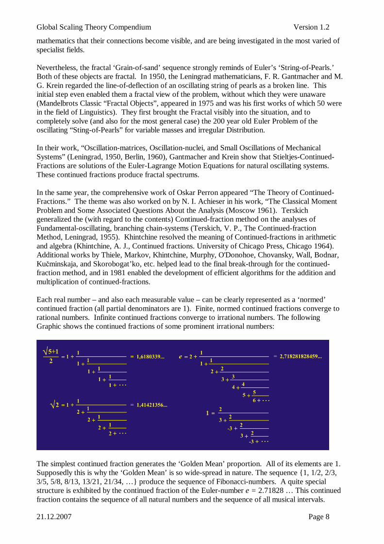
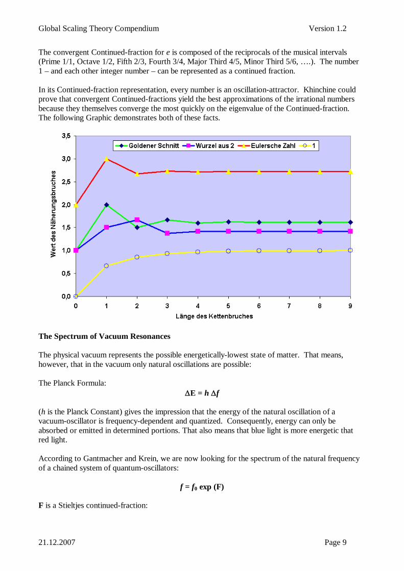
Each real number – and also each measurable value – can be clearly represented as a ‘normed’continued fraction (all partial denominators are 1). Finite, normed continued fractions converge torational numbers. Infinite continued fractions converge to irrational numbers. The followingGraphic shows the continued fractions of some prominent irrational numbers:

The simplest continued fraction generates the ‘Golden Mean’ proportion. All of its elements are 1.Supposedly this is why the ‘Golden Mean’ is so wide-spread in nature. The sequence {1, 1/2, 2/3,3/5, 5/8, 8/13, 13/21, 21/34, …} produce the sequence of Fibonacci-numbers. A quite specialstructure is exhibited by the continued fraction of the Euler-number e = 2.71828 … This continuedfraction contains the sequence of all natural numbers and the sequence of all musical intervals.


21.12.2007

The convergent Continued-fraction for e is composed of the reciprocals of the musical intervals(Prime 1/1, Octave 1/2, Fifth 2/3, Fourth 3/4, Major Third 4/5, Minor Third 5/6, ….). The number1 – and each other integer number – can be represented as a continued fraction.

In its Continued-fraction representation, every number is an oscillation-attractor. Khinchine couldprove that convergent Continued-fractions yield the best approximations of the irrational numbersbecause they themselves converge the most quickly on the eigenvalue of the Continued-fraction.The following Graphic demonstrates both of these facts.

The Spectrum of Vacuum Resonances

The physical vacuum represents the possible energetically-lowest state of matter. That means,however, that in the vacuum only natural oscillations are possible:

The Planck Formula:E = h f

(h is the Planck Constant) gives the impression that the energy of the natural oscillation of avacuum-oscillator is frequency-dependent and quantized. Consequently, energy can only beabsorbed or emitted in determined portions. That also means that blue light is more energetic thatred light.

According to Gantmacher and Krein, we are now looking for the spectrum of the natural frequencyof a chained system of quantum-oscillators:

f = f0 exp (F)

F is a Stieltjes continued-fraction:


21.12.2007

Natural oscillations occur at the energetically lowest possible level and, therefore, lose little energy.Consequently, natural oscillations very strongly fulfill the laws of energy conservation.

For this reason, the chained system of quantum-oscillators possesses a standard spectrum with aminimal level quantization and a continuous occupation. For the Stieltjes continued-fraction thatmeans:

Z =2| N0 | = 0, 1, 2, 3, ...| Ni > 0 | = 1, 2, 3, ...

The convergence criterion for Stieltjes continued-fractions requires that

| Ni > 0 | | Z | +1

Attractor-values of the continued-fraction fulfill the condition:

| Ni | = ( | Z | +1 ) mm = 0, 1, 2, ... für i = 0m = 1, 2, 3, ... für i > 0

The Stieltjes continued-fraction

with the partial denominator Z = 2 generates the logarithmic-fractal spectrum of the naturalfrequencies of the chained system of quantum-oscillators:

Die quantum-numbers N0, N1, N2, for layers i = 0, 1, 2, ... take on a integer number value:

| N0 | = 0, 1, 2, 3, ...| Ni > 0 | = 1, 2, 3, ...

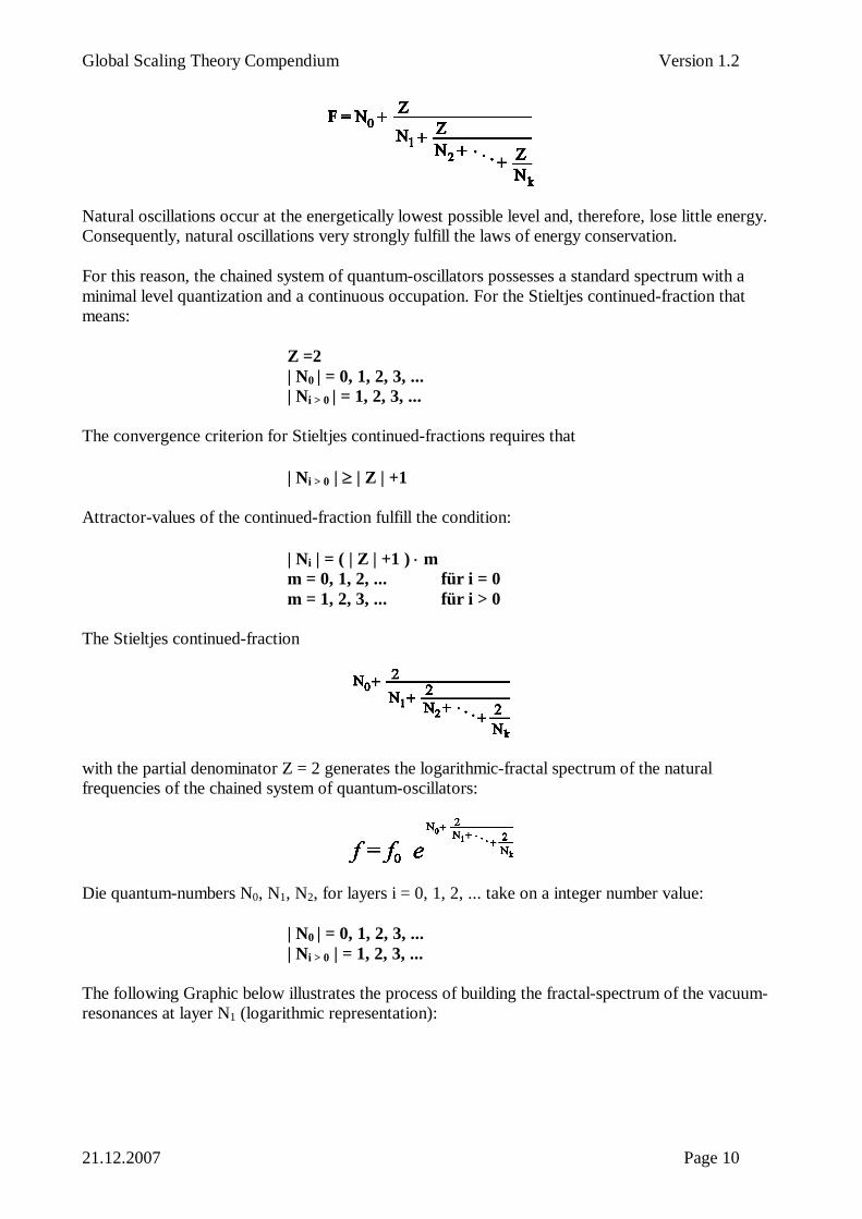
The following Graphic below illustrates the process of building the fractal-spectrum of the vacuum-resonances at layer N1 (logarithmic representation):


21.12.2007

The quantum-numbers N1 run through all positive as well as negative integer numbers. Areas ofmaximal spectral-density arise automatically in intervals of 3 logarithmic units:

For all | Ni | = 3j (j = 1, 2, 3, ...), the spectral-density reaches a local (at layer i) maximum. In theareas between | Ni | = 3j – 2 to | Ni | = 3j – 1 for i > 0, the spectral-density is minimal. Areas ofmaximal spectral-density are indicated as Nodes, areas of minimal spectral-density are indicated asGaps in the Spectrum.

In quantum physics, The Heisenberg ‘uncertainty’ relation, below, defines the proportionalrelationship of complementary measurands, for example, the uncertainty of the place x and theimpulse p of a particle that is moving in the direction x:

x p h/4

Uncertainty relations also exist between many other pairs of quantum-physical measurands.Generally, for each quantum-physical measurand, one finds its complementary measurand.

In the natural-oscillation-mode (before and after measurement), the phase-shift of the spectrumamounts to a complementary measurand is | | = 3/2. Accordingly, when a quantum physicalmeasurand reaches a minimum absolute value, the complementary measurand runs through amaximum absolute value:

The overlapping areas of the complementary spectrum are marked in green:


21.12.2007

The more layers calculated, the more clearly the fine structure of the spectrum can be recognized.

Major-quantum-numbers, divisible by 3 without remainder | N0 | = 3j, are spectrum Major-nodes,and, divisible by 3 without remainder Sub-quantum-numbers | N1 | = 3j, are spectrum Sub-nodes, allother Sub-quantum numbers | N1 | 3j indicate the boundaries of Sub-gaps.

The Proton Resonance Spectrum

Whether atom, planetary system, or Milky Way - over 99 percent of the volume of normal matterconsists of vacuum (particle-free physical fields). Elementary particles, from which matter consists,are Vacuum-resonances, and consequently Oscillation-nodes, Attractors, and singularities of thevacuum.

Vacuum-resonance is one of the most important mechanisms, which regulates the harmonicorganization of matter at all levels (scales) – from the sub-atomic particles to the galaxies. As this isa matter of harmonic oscillations, one speaks of the “Melody of Creation.”

The Proton is, by far, the most stable Vacuum-resonance. Its life-span exceeds everythingimaginable, exceeding one-hundred-thousand billion billion billion (1032) years. No one knows theactual life-span of a Proton. No scientist could ever witness the decay of a Proton.

The unusually high life-span of the Proton is the reason why over 99 percent of matter’s massconsists of Protons and Proton Resonances - Nucleons.

That is why Proton Resonances determine the course of all processes and the composition of allstructures in the universe.

The objective of Global Scaling Theory is the Spectrum of Proton-resonances. As spectrum ofnatural-oscillation-processes, it is fractal, that means fragmentary, similarly which is itself andlogarithmically scale-invariant.

Global Scaling Theory sees in logarithmic scale-invariance of the Spectrum of Proton-resonancesthe origin of the Global Scaling phenomenon – the logarithmic scale-invariance in the compositionof matter.


21.12.2007

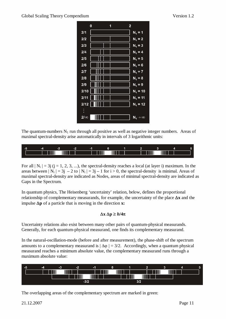
Algebraically, the logarithmic spectrum of the Proton-resonances is described by the Global Scalingcontinued-fraction:

fP = 1.425486... x 1024 Hz is the natural frequency of the Proton, f is the frequency of a proton-resonance. In the natural-oscillation-mode, the phase-angle can only assume the value = {0;3/2}, N0 and the partial denominators N1, ... are integer numbers (Quantum-numbers). Partialdenominators, whose values are multiples of 3, correspond to Nodes in the Spectrum. All other(integer number) values correspond to Gap-boundaries. The Spectrum of Proton-resonances is theFundamental-Fractal of the Global Scaling Theory.

Global Scaling Theory is based on the quantum metrology of the Proton. The values of the basicphysical constants (Rest-mass of the Proton mp, and Planck-constant h, Speed-of-light in theVacuum c, Boltzmann-constant k, and Fundamental Electrical Charge e) and the transcendentalnumbers e = 2.71828... and = 3.14159 are the uniquely physical standard parameters of thetheory.

The Quantum Metrology of the Proton

rest mass mp 1.672621... 10-27 kgnatural wavelength p = h / 2 mp 2.103089... 10-16 m

natural frequency fp = c / p 1.425486... 1024 Hz

natural oscillation period p = 1 / fp 7.01515... 10-25 s

natural energy Ep = mp c2 9.38272... 108 eVnatural temperature Tp = mp c2 / k 1.08881... 1013 Kelectrical charge ep 1.6021764...10-19 C

The Fundamental Fractal not only describes the Spectrum of Proton-resonance-frequencies, but alsothe Proton-resonance-period-spectrum, - Energy-spectrum, - Mass-spectrum, - Velocity-spectrum,Temperature-spectrum, - Pressure-spectrum, Electrical-charge-quantity-spectrum, etc.

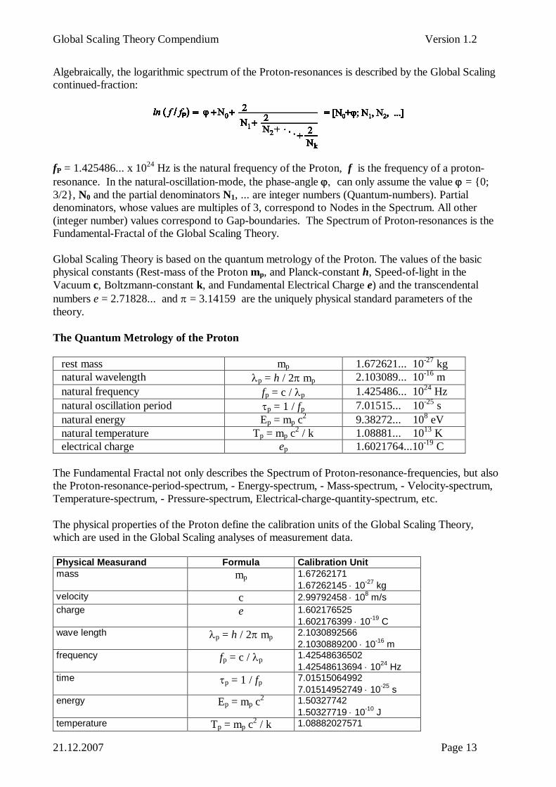
The physical properties of the Proton define the calibration units of the Global Scaling Theory,which are used in the Global Scaling analyses of measurement data.

Physical Measurand Formula Calibration Unitmass mp 1.67262171

1.67262145 10-27

kgvelocity c 2.99792458 10

8m/s

charge e 1.6021765251.602176399 10

-19C

wave length p = h / 2 mp2.10308925662.1030889200 10

-16m

frequency fp = c / p1.425486365021.42548613694 10

24Hz

time p = 1 / fp7.015150649927.01514952749 10

-25s

energy Ep = mp c2 1.503277421.50327719 10

-10J

temperature Tp = mp c2 / k 1.08882027571


21.12.2007

1.08881639695 1013

Kforce Fp = mp c2 / 7.14794990157

7.14794764678 105

Npressure Pp = Fp / p

1.616092553881.61609152693 10

37N/m

2

electrical current intensity Ip = e fp 2.28388079072.2838802457 10

5A

electrical voltage Up = Ep / e 9.38272105919.3827188627 10

8V

electrical resistance Rp = Up / Ip 4.10823688184.1082349398 10

3

electrical capacity Cp = e / Up 1.70758236331.7075818293 10

-28F

Global Scaling Methods of Research and Development

Global Scaling Analysis

Global Scaling Analysis begins with the localization of reproduceable measure-values in thecorrespondingly calibrated Proton-resonance-spectrum. Mathematically, this first stage in GlobalScaling analysis consists of the following steps:

1. One divides the measure-value by the corresponding Proton calibration unit.Example: GS-Analysis of the wavelength = 540 nm:

/ p = 540 10-9

m / 2,103089... 10-16

m = 2,56765... 109

2. The logarithm of the result based on e = 2,71828... is calculated:

ln (2,56765... 109) = 21,666...

3. The logarithm is decomposed into a Global Scaling Continued-fraction:

21,666... = 0 + 21 + 2/3 = [21+0; 3]

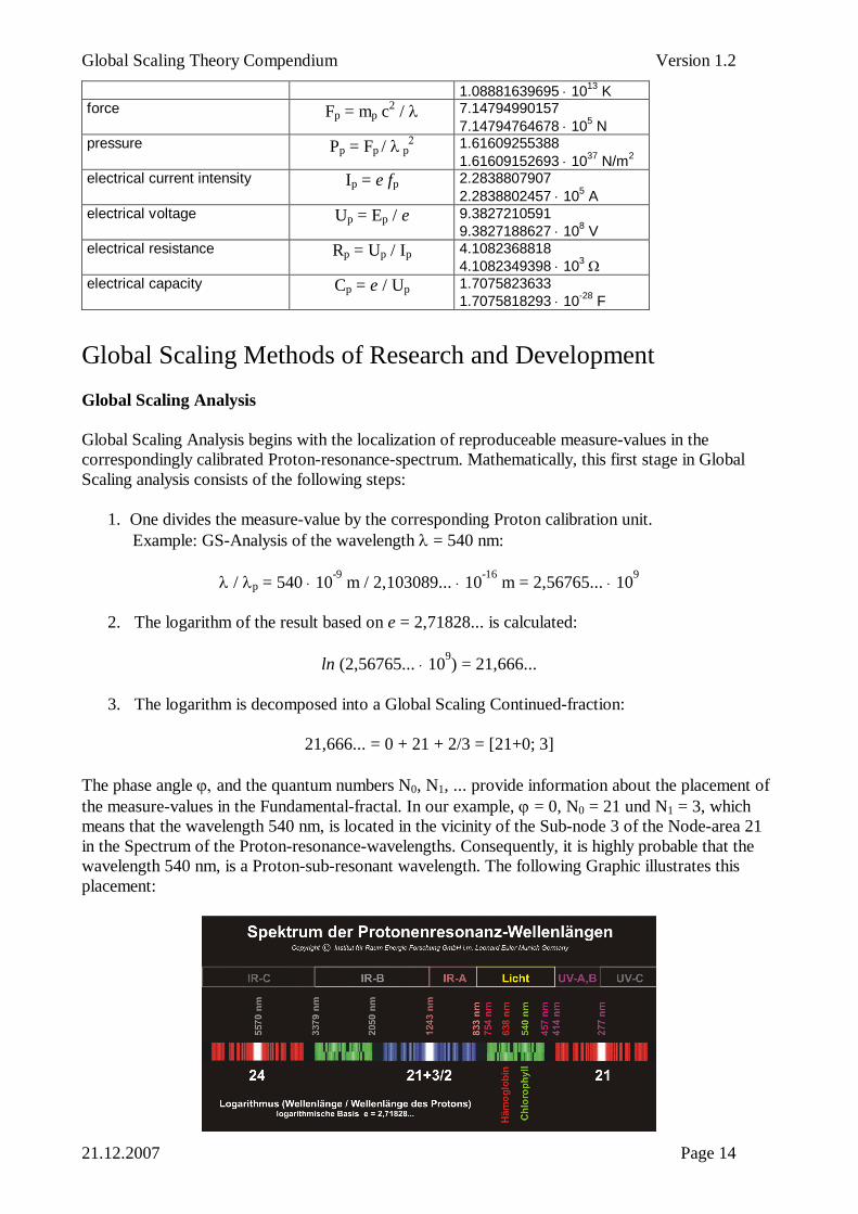
The phase angle and the quantum numbers N0, N1, ... provide information about the placement ofthe measure-values in the Fundamental-fractal. In our example, = 0, N0 = 21 und N1 = 3, whichmeans that the wavelength 540 nm, is located in the vicinity of the Sub-node 3 of the Node-area 21in the Spectrum of the Proton-resonance-wavelengths. Consequently, it is highly probable that thewavelength 540 nm, is a Proton-sub-resonant wavelength. The following Graphic illustrates thisplacement:


21.12.2007

Visible light covers the green area (area of higher process complexity and higher influence /sensitivity) between the Proton-resonances [24+3/2] and [21].

The reflection maximum for eukariotic cells at 1250 nm, and the absorption maximum forprokariotic cells at 280 nm are, consequently, with high probability, Proton-resonance wave lengths.It means that these reflections and absorptions, with high probability, are based on Proton resonanceprocesses.

The placement of reproduceable measure-values in the Fundamental Fractal provides explanationabout the state of a system or the stage of a process.

If the measure-values relevant to a process lie in a Gap of the Fundamental Fractal, then theprocess, with high probability, is not in the Proton-resonance-modus and, with high probability,runs through a laminar phase.

If the measure-values relevant to a process lie in the vicinity of a Node (place of high spectraldensity) in the Fundamental Fractal, then the process is in the Proton-resonance-modus and, withhigh probability, runs through a turbulent phase.

If the measure-values relevant to a process stay in the vicinity of a Node, then the process, with highprobability, is located in a relatively early phase of its development.

If the measure-values relevant to a process stabilize on the border of a Node area, for example onthe border of a Gap in the Fundamental Fractal, then the process, with high probability, is located ina relatively late phase of its development.

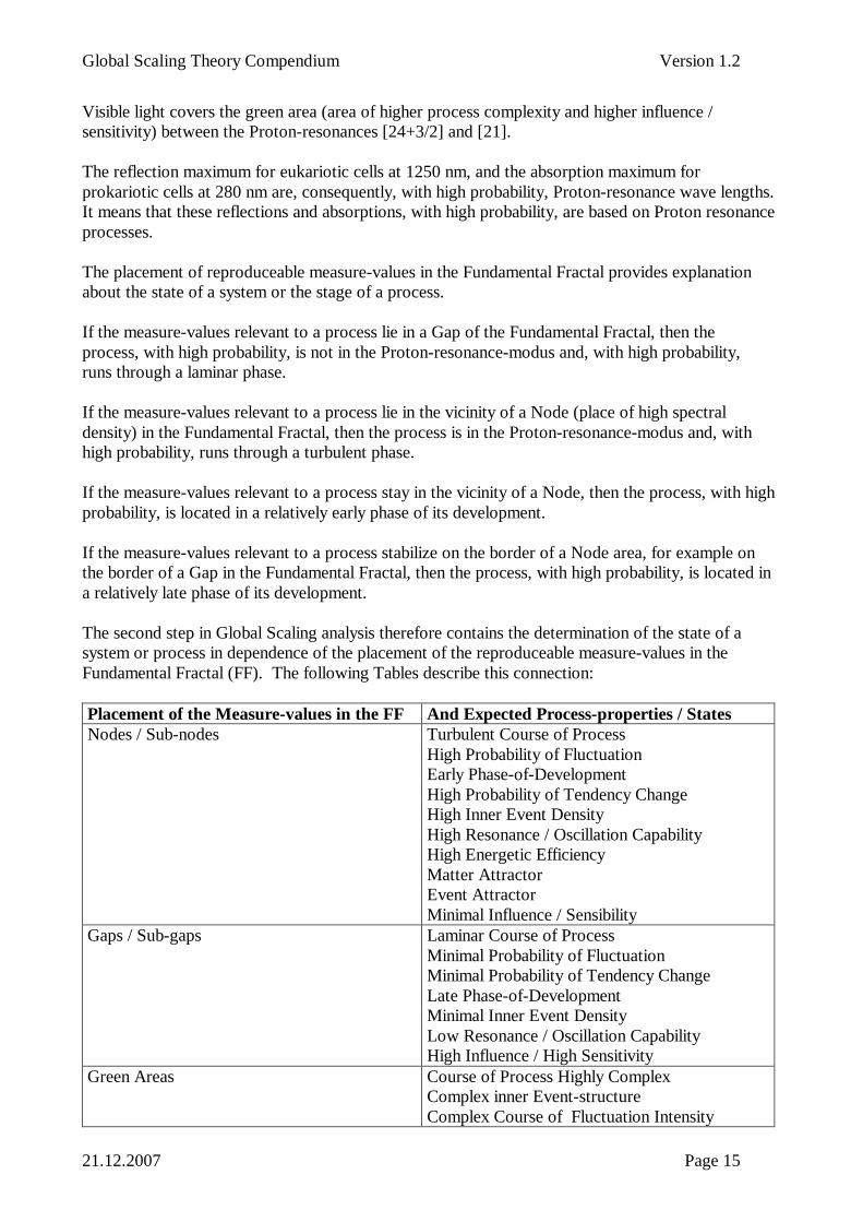
The second step in Global Scaling analysis therefore contains the determination of the state of asystem or process in dependence of the placement of the reproduceable measure-values in theFundamental Fractal (FF). The following Tables describe this connection:

Placement of the Measure-values in the FF And Expected Process-properties / StatesNodes / Sub-nodes Turbulent Course of Process

High Probability of FluctuationEarly Phase-of-DevelopmentHigh Probability of Tendency ChangeHigh Inner Event DensityHigh Resonance / Oscillation CapabilityHigh Energetic EfficiencyMatter AttractorEvent AttractorMinimal Influence / Sensibility

Gaps / Sub-gaps Laminar Course of ProcessMinimal Probability of FluctuationMinimal Probability of Tendency ChangeLate Phase-of-DevelopmentMinimal Inner Event DensityLow Resonance / Oscillation CapabilityHigh Influence / High Sensitivity

Green Areas Course of Process Highly ComplexComplex inner Event-structureComplex Course of Fluctuation Intensity


21.12.2007

Laminar Course of Process / Weak TurbulenceHigh Influence / High SensitivityMean Phase-of-Development

Gap Borders Beginning of the compression of event densityEnd of the decompression of the event densityBeginning / Breaking-off of an Event ChainDevelopment limitEvolution AttractorHigh Phase-of-Development

If process relevant, reproduceable measure-values move through the Fundamental Fractal during thecourse of a process, it is highly-probable that the character of the process will also change. Thefollowing Table describes this connection.

Direction-of-Movement of theMeasure-Values in the FF

Expected Process-properties / States

Increasing Spectral-density(Compression)

Increasing Probability of FluctuationsIncreasing Probability of TurbulenceIncreasing Probability of Trend ChangeIncreasing Energetic EfficiencyIncreasing Inner Event DensityIncreasing Complexity in Process CourseIncreasing Resonance / Oscillation-CapabilityHigh Probability of Fusion

Decreasing Spectral-density (Decompression) Decreasing Probability of FluctuationsDecreasing Probability of TurbulenceDecreasing Probability of Trend ChangeDecreasing Energetic EfficiencyDecreasing Inner Event DensityDecreasing Complexity in Process CourseDecreasing Resonance / Oscillation-CapabilityHigh Probability of Matter Decay

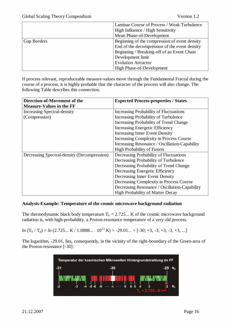
Analysis-Example: Temperature of the cosmic microwave background radiation

The thermodynamic black body temperature Tk = 2.725... K of the cosmic microwave backgroundradiation is, with high-probability, a Proton-resonance temperature of a very old process.

ln (Tk / Tp) = ln (2.725... K / 1.0888... 1013 K) = -29.01... = [-30; +3, -3, +3, -3, +3, ...]

The logarithm, -29.01, lies, consequently, in the vicinity of the right-boundary of the Green-area ofthe Proton-resonance [-30]:


21.12.2007

The most exterior boundary of the Green-area denotes a Proton-resonance limit temperature value(Evolution Attractor).

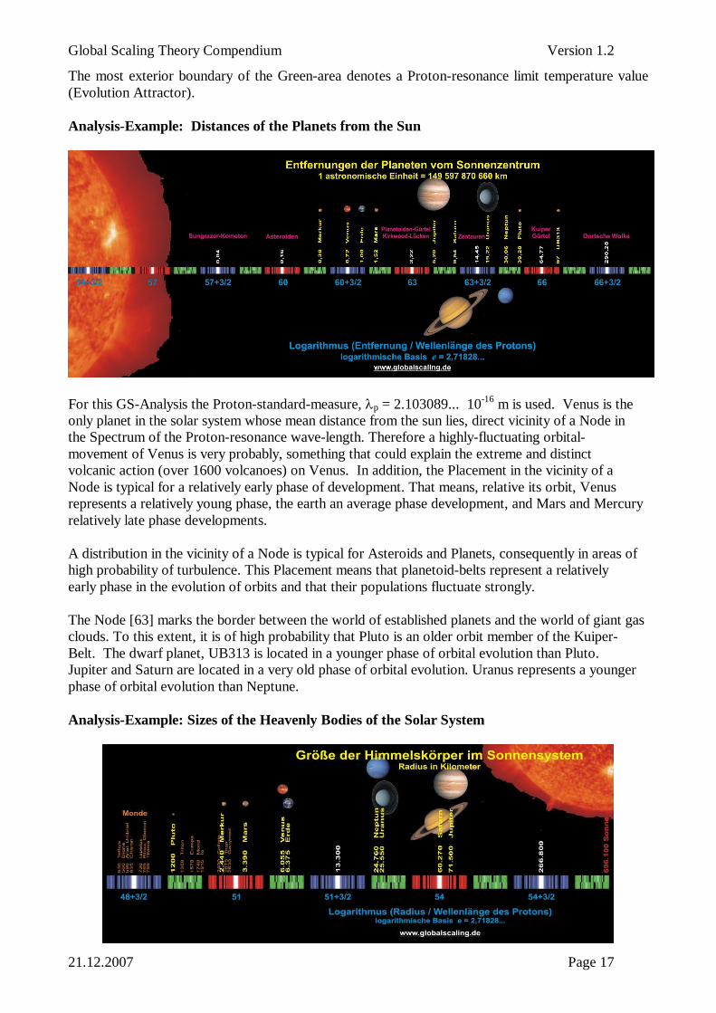
Analysis-Example: Distances of the Planets from the Sun

For this GS-Analysis the Proton-standard-measure, p = 2.103089... 10-16 m is used. Venus is theonly planet in the solar system whose mean distance from the sun lies, direct vicinity of a Node inthe Spectrum of the Proton-resonance wave-length. Therefore a highly-fluctuating orbital-movement of Venus is very probably, something that could explain the extreme and distinctvolcanic action (over 1600 volcanoes) on Venus. In addition, the Placement in the vicinity of aNode is typical for a relatively early phase of development. That means, relative its orbit, Venusrepresents a relatively young phase, the earth an average phase development, and Mars and Mercuryrelatively late phase developments.

A distribution in the vicinity of a Node is typical for Asteroids and Planets, consequently in areas ofhigh probability of turbulence. This Placement means that planetoid-belts represent a relativelyearly phase in the evolution of orbits and that their populations fluctuate strongly.

The Node [63] marks the border between the world of established planets and the world of giant gasclouds. To this extent, it is of high probability that Pluto is an older orbit member of the Kuiper-Belt. The dwarf planet, UB313 is located in a younger phase of orbital evolution than Pluto.Jupiter and Saturn are located in a very old phase of orbital evolution. Uranus represents a youngerphase of orbital evolution than Neptune.

Analysis-Example: Sizes of the Heavenly Bodies of the Solar System


21.12.2007

For this GS-Analysis the Proton calibration unit p = 2.103089... 10-16 m is used. Saturn and Jupiterare located in a relatively young phase in the evolution of their sizes. Saturn is located just a little tothe right of Node [54], Jupiter somewhat further to the right, and Saturn and Jupiter, with highprobability, therefore become essentially larger. Uranus and Neptune represent an essential laterphase of the evolution of the giant gas clouds than Jupiter and Saturn. In the solar system, the Node[51+3/2] separates the world of established planets from the world of the giant gas clouds. Mercuryand Mars represent a relatively early phase of size evolution, and Pluto represents, essentially, anolder one. This also holds for our moon as well as for the Neptune Moon, Triton, and for theJupiter Moons, Europa and Io. The sun finds itself, in the evolution of its size, in a relatively latephase. It is highly probable that the sun will become larger, whereby its radius will reach amaximum, [54+3/2; 2] 725260 km; after which, with high probability, it will not essentiallychange for a long time.

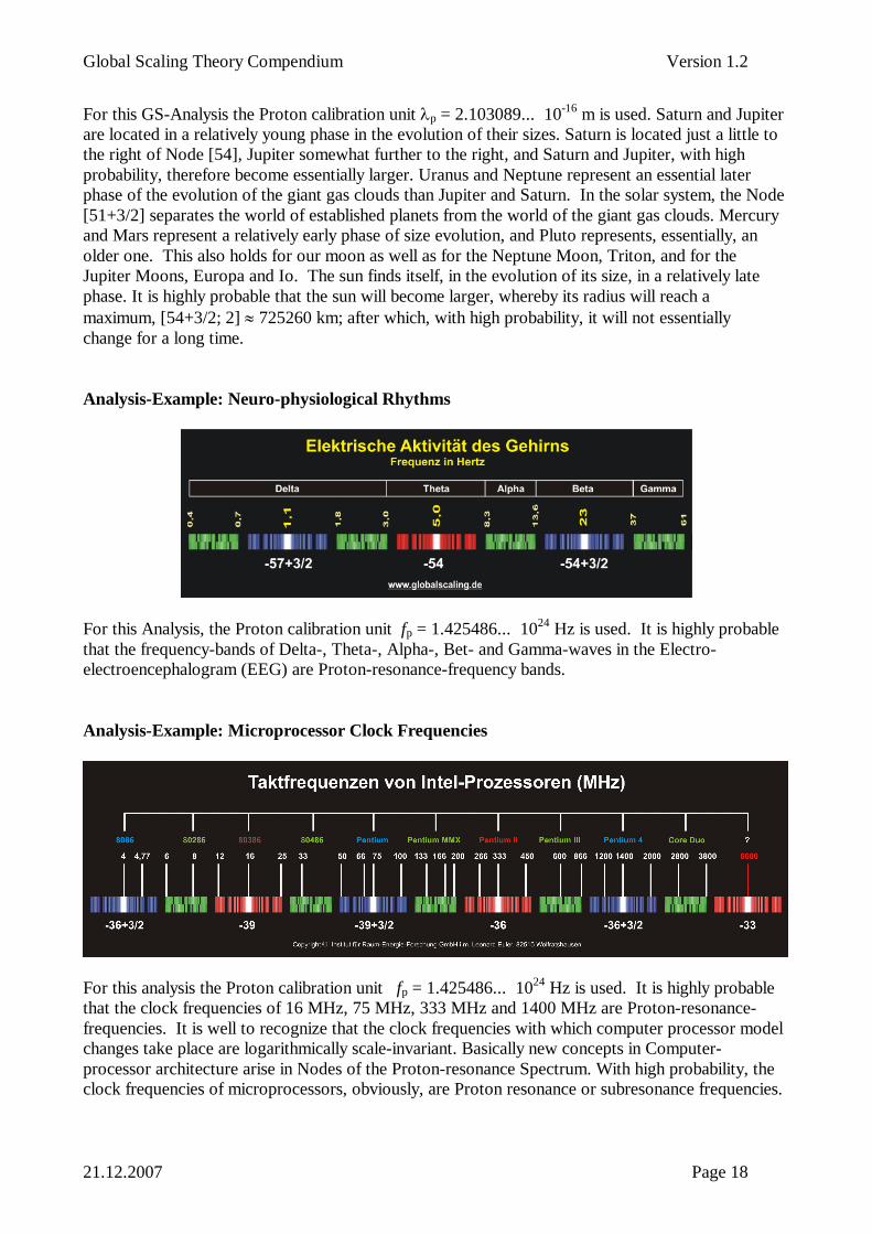
Analysis-Example: Neuro-physiological Rhythms

For this Analysis, the Proton calibration unit fp = 1.425486... 1024 Hz is used. It is highly probablethat the frequency-bands of Delta-, Theta-, Alpha-, Bet- and Gamma-waves in the Electro-electroencephalogram (EEG) are Proton-resonance-frequency bands.

Analysis-Example: Microprocessor Clock Frequencies

For this analysis the Proton calibration unit fp = 1.425486... 1024 Hz is used. It is highly probablethat the clock frequencies of 16 MHz, 75 MHz, 333 MHz and 1400 MHz are Proton-resonance-frequencies. It is well to recognize that the clock frequencies with which computer processor modelchanges take place are logarithmically scale-invariant. Basically new concepts in Computer-processor architecture arise in Nodes of the Proton-resonance Spectrum. With high probability, theclock frequencies of microprocessors, obviously, are Proton resonance or subresonance frequencies.


21.12.2007

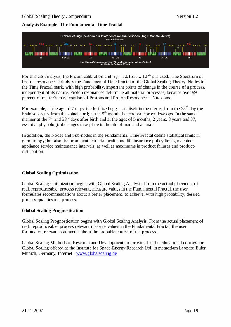
Analysis Example: The Fundamental Time Fractal

For this GS-Analysis, the Proton calibration unit p = 7.01515... 10-25 s is used. The Spectrum ofProton-resonance-periods is the Fundamental Time Fractal of the Global Scaling Theory. Nodes inthe Time Fractal mark, with high probability, important points of change in the course of a process,independent of its nature. Proton resonances determine all material processes, because over 99percent of matter’s mass consists of Protons and Proton Resonances - Nucleons.

For example, at the age of 7 days, the fertilized egg nests itself in the uterus; from the 33rd day thebrain separates from the spinal cord; at the 5th month the cerebral cortex develops. In the samemanner at the 7th and 33rd days after birth and at the ages of 5 months, 2 years, 8 years and 37,essential physiological changes take place in the life of man and animal.

In addition, the Nodes and Sub-nodes in the Fundamental Time Fractal define statistical limits ingerontology; but also the prominent actuarial health and life insurance policy limits, machineappliance service maintenance intervals, as well as maximums in product failures and product-distribution.

Global Scaling Optimization

Global Scaling Optimization begins with Global Scaling Analysis. From the actual placement ofreal, reproduceable, process relevant, measure values in the Fundamental Fractal, the userformulates recommendations about a better placement, to achieve, with high probability, desiredprocess-qualities in a process.

Global Scaling Prognostication

Global Scaling Prognostication begins with Global Scaling Analysis. From the actual placement ofreal, reproduceable, process relevant measure values in the Fundamental Fractal, the userformulates, relevant statements about the probable course of the process.

Global Scaling Methods of Research and Development are provided in the educational courses forGlobal Scaling offered at the Institute for Space-Energy Research Ltd. in memoriam Leonard Euler,Munich, Germany, Internet: www.globalscaling.de

http://www.globalscaling.de/


21.12.2007

Global Scaling Applications

Global Scaling in Medicine

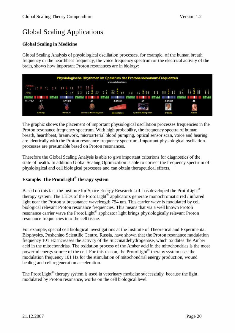
Global Scaling Analysis of physiological oscillation processes, for example, of the human breathfrequency or the hearthbeat frequency, the voice frequency spectrum or the electrical activity of thebrain, shows how important Proton resonances are in biology:

The graphic shows the placement of important physiological oscillation processes frequencies in theProton resonance frequency spectrum. With high probability, the frequency spectra of humanbreath, hearthbeat, brainwork, microarterial blood pumping, optical sensor scan, voice and hearingare identically with the Proton resonance frequency spectrum. Important physiological oscillationprocesses are presumable based on Proton resonances.

Therefore the Global Scaling Analysis is able to give important criterions for diagnostics of thestate of health. In addition Global Scaling Optimization is able to correct the frequency spectrum ofphysiological and cell biological processes and can obtain therapeutical effects.

Example: The ProtoLight therapy system

Based on this fact the Institute for Space Energy Research Ltd. has developed the ProtoLight

therapy system. The LEDs of the ProtoLight applicators generate monochromatic red / infraredlight near the Proton subresonance wavelength 754 nm. This carrier wave is modulated by cellbiological relevant Proton resonance frequencies. This means that via a well known Protonresonance carrier wave the ProtoLight applicator light brings physiologically relevant Protonresonance frequencies into the cell tissue.

For example, special cell biological investigations at the Institute of Theoretical and ExperimentalBiophysics, Pushchino Scientific Centre, Russia, have shown that the Proton resonance modulationfrequency 101 Hz increases the activity of the Succinatdehydrogenase, which oxidates the Amberacid in the mitochondrias. The oxidation process of the Amber acid in the mitochondrias is the mostpowerful energy source of the cell. For this reason, the ProtoLight therapy system uses themodulation frequency 101 Hz for the stimulation of mitochondrial energy production, woundhealing and cell regeneration acceleration.

The ProtoLight therapy system is used in veterinary medicine successfully. because the light,modulated by Proton resonance, works on the cell biological level.


21.12.2007

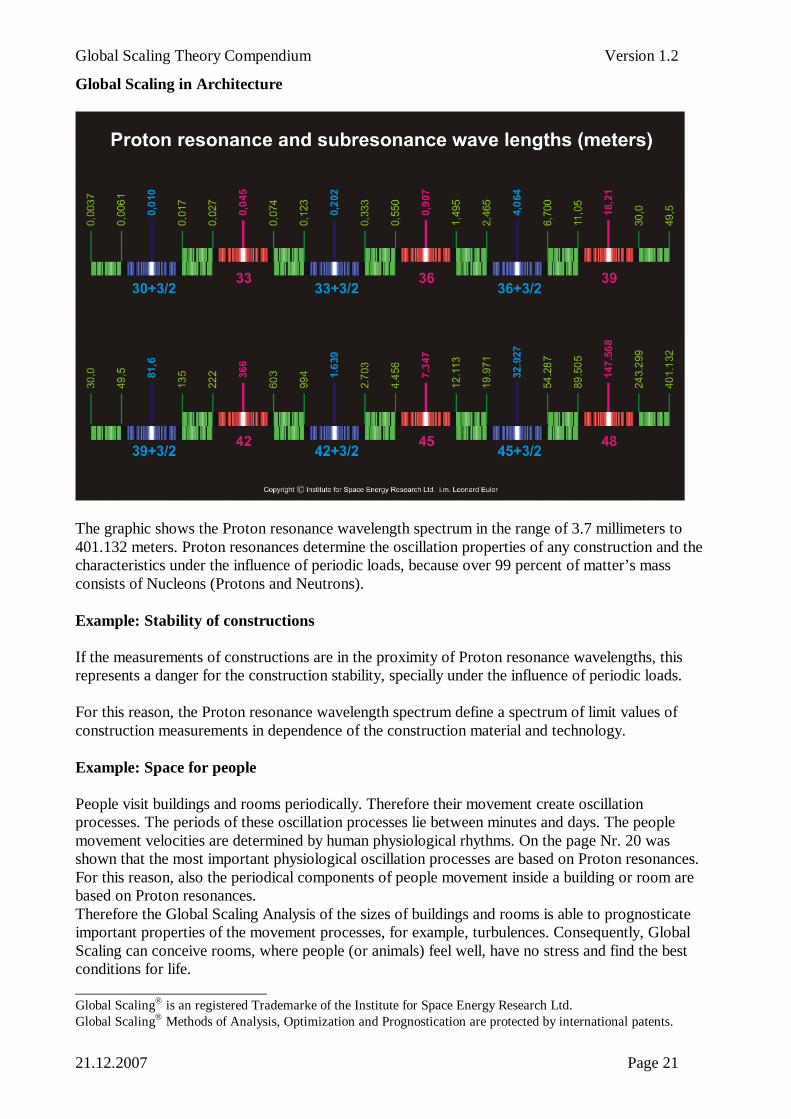
Global Scaling in Architecture

The graphic shows the Proton resonance wavelength spectrum in the range of 3.7 millimeters to401.132 meters. Proton resonances determine the oscillation properties of any construction and thecharacteristics under the influence of periodic loads, because over 99 percent of matter’s massconsists of Nucleons (Protons and Neutrons).

Example: Stability of constructions

If the measurements of constructions are in the proximity of Proton resonance wavelengths, thisrepresents a danger for the construction stability, specially under the influence of periodic loads.

For this reason, the Proton resonance wavelength spectrum define a spectrum of limit values ofconstruction measurements in dependence of the construction material and technology.

Example: Space for people

People visit buildings and rooms periodically. Therefore their movement create oscillationprocesses. The periods of these oscillation processes lie between minutes and days. The peoplemovement velocities are determined by human physiological rhythms. On the page Nr. 20 wasshown that the most important physiological oscillation processes are based on Proton resonances.For this reason, also the periodical components of people movement inside a building or room arebased on Proton resonances.Therefore the Global Scaling Analysis of the sizes of buildings and rooms is able to prognosticateimportant properties of the movement processes, for example, turbulences. Consequently, GlobalScaling can conceive rooms, where people (or animals) feel well, have no stress and find the bestconditions for life.________________________Global Scaling is an registered Trademarke of the Institute for Space Energy Research Ltd.Global Scaling Methods of Analysis, Optimization and Prognostication are protected by international patents.

necesitate contraunda lege3 newton

Documents

global scaling munich

processindependent scaling

critical scaling levels

logarithmic world

chemical processes

macroscopic processes

oscillatory processes

metabolic processes