NBER WORKING PAPER SERIES

VENTURE CAPITAL CONTRACTING ANDSYNDICATION: AN EXPERIMENT IN

COMPUTATIONAL CORPORATE FINANCE

Zsuzsanna FluckKedran GarrisonStewart C. Myers

Working Paper 11624http://www.nber.org/papers/w11624

NATIONAL BUREAU OF ECONOMIC RESEARCH1050 Massachusetts Avenue

Cambridge, MA 02138September 2005

We are grateful for helpful comments from Ulf Axelson, Amar Bhide, Francesca Cornelli, Paul Gompers,Steve Kaplan, Josh Lerner, Tom Noe, David Scharfstein, Per Str¡§omberg, Michael Weisbach andparticipants at presentations at LSE, MIT, Michigan State University, the University of Minnesota, theConference on Venture Capital and Private Equity (Stockholm), the Financial Intermediation ResearchSociety Conference (Capri) and the American Finance Association meetings (Philadelphia). The viewsexpressed herein are those of the author(s) and do not necessarily reflect the views of the National Bureauof Economic Research.

©2005 by Zsuzsanna Fluck, Kedran Garrison and Stewart C. Myers. All rights reserved. Short sections oftext, not to exceed two paragraphs, may be quoted without explicit permission provided that full credit,including © notice, is given to the source.

Venture Capital Contracting and Syndication: An Experiment in Computational CorporateFinanceZsuzsanna Fluck, Kedran Garrison and Stewart C. MyersNBER Working Paper No. 11624September 2005JEL No. G24, G32

ABSTRACT

This paper develops a model to study how entrepreneurs and venture-capital investors deal with

moral hazard, effort provision, asymmetric information and hold-up problems. We explore several

financing scenarios, including first-best, monopolistic, syndicated and fully competitive financing.

We solve numerically for the entrepreneur's effort, the terms of financing, the venture capitalist's

investment decision and NPV. We find significant value losses due to holdup problems and under-

provision of effort that can outweigh the benefits of staged financing and investment. We show that

a commitment to later-stage syndicate financing increases effort and NPV and preserves the option

value of staged investment. This commitment benefits initial venture capital investors as well as the

entrepreneur.

Zsuzsanna Fluck Michigan State UniversityDepartment of Finance Graduate School of Management315 Eppley CenterEast Lansing, MI 48824-1122fluck@bus.msu.edu

Kedran Garrison MIT - EFA77 Massachusetts AvenueCambridge, MA 02139-4307garrisk@mit.edu

Stewart C. MyersSloan School of ManagementMIT, Room E52-45150 Memorial DriveCambridge, MA 02142-1347and NBERscmyers@mit.edu

1 Introduction

This paper develops a model to study how entrepreneurs and venture-capital investors dealwith effort provision, moral hazard, asymmetric information and hold-up problems whencontracts are incomplete and investment proceeds in stages. How much value is lost in theentrepreneur-venture capital relationship relative to first-best value? How does the valuelost depend on risk and the time-pattern of required investment? What determines whethera positive-NPV project can in fact be financed? What are the advantages and disadvantagesof staged financing? Are there significant efficiency gains from syndication of later-stagefinancing?

We argue that these and related questions should not be analyzed one by one, butjointly in a common setting. Some features of venture-capital contracting may not solve aparticular problem, but instead trade off one problem against another. For example, a studythat focused just on the option-like advantages of staged investment could easily miss thecosts of staging, particularly the negative feedback to effort if venture-capital investors canhold up the entrepreneur by dictating financing terms in later stages. (We find many caseswhere hold-up costs outweigh the advantages of staged financing and full upfront financingactually increases value.)

A joint analysis of the problems inherent in the entrepreneur-venture capital relationshipdoes not lead to closed-form solutions or simple theorems. Therefore we embark on anexperiment in computational corporate finance, which is the formal study of financing andinvestment problems that do not have closed-form solutions.1 We believe the time is ripefor a computational model of venture capital. Venture-capital institutions, contracts andprocedures were well documented more than a decade ago. It was clear then that the agencyand information problems encountered in ordinary financing decisions are especially acutein venture capital. The successes of venture capital have stimulated theoretical work on howthese problems are mitigated. But most theoretical papers have focused on only one problemor tradeoff and run the risk of missing the bigger picture.

Of course the breadth and richness of a computational model do not come free, andnumerical results are never absolutely conclusive. One can never rule out the possibilitythat results would have been different with different inputs or modeling choices. But ourmodel, though simplified, follows actual practice in venture capital. We have verified ourmain results over a wide range of inputs. We believe our results help to clarify why venture-capital investment works when it works and why it sometimes fails.

The structure of venture-capital financing is known frommany sources, including Sahlman(1990), Lerner (1994), Fenn, Liang and Prowse (1995), Gompers (1995), Gompers and Lerner(1996, 2002), Hellman and Puri (2000, 2002) and Kaplan and Stromberg (2003). We willpreview our model and results after a brief review of the features of venture-capital con-tracting that are most important to our paper. The review includes comments on related

1Computational models are frequently used to understand the value of real and financial options, buttheir use on the financing side of corporate balance sheets is an infant industry. The short list of com-putational papers on financing includes Mello and Parsons (1992), Leland (1994, 1998), Boyd and Smith(1994), Parrino and Weisbach (1999), Robe (1999, 2001), Parrino, Poteshman and Weisbach (2002) and Ju,Parrino, Poteshman and Weisbach (2004). These papers explore the tradeoff theory of capital structure andthe risk-shifting incentives created by debt financing.

1

theoretical work.

1.1 Venture capital contracting

Venture capital brings together one or more entrepreneurs, who contribute ideas, plans, hu-man capital and effort, and private investors, who contribute experience, expertise, contactsand most of the money. For simplicity, we will refer to one entrepreneur and to one initialventure-capital investor. Their joint participation creates a two-way incentive problem. Theinvestor has to share financial payoffs with the entrepreneur in order to secure her commit-ment and effort. Thus the investor may not be willing to participate even if the startup haspositive overall NPV. Second, the entrepreneur will underinvest in effort if she has to shareher marginal value added with the investor.2

1.1.1 Sweat equity

The entrepreneur invests even when she puts up none of the financing. She contributes hereffort and absorbs part of the firm’s business risk. The difference between her salary andher outside compensation is an opportunity cost. Specialization of her human capital to thenew firm also creates an opportunity cost if the firm fails.3

The entrepreneur receives shares in exchange for these investments. These shares may notvest immediately, and they are illiquid unless and until the firm is sold or goes public.4 Theventure capitalist frequently requires the entrepreneur to sign a contract that precludes workfor a competitor. The entrepreneur therefore has a strong incentive to stick with the firmand make it successful. In our model, the entrepreneur contributes no financial investmentand is willing to continue so long as the present value of her shares exceeds her costs of effort.

1.1.2 Staged investment and financing

A startup is a compound call option. Financing and investment are made in stages. Thestages match up with business milestones, such as a demonstration of technology or a suc-cessful product introduction.

We assume that the entrepreneur and venture capitalist cannot write a complete contractto specify the terms of future financing. The terms are determined by bargaining as financingis raised stage by stage. If additional investors join in later stages, the bargain has to beacceptable to them as well as the entrepreneur and initial venture capitalist.

The option value added by staging is obvious, but staging may also serve other purposes.In Bergemann and Hege (1998) and Noldeke and Schmidt (1998), staging allows the venturecapitalist to learn the startup’s value and thereby induce the entrepreneur’s effort. In Neher

2This is an extreme version of Myers’s (1977) underinvestment problem.3This opportunity cost could perhaps be reduced if new ventures are developed as divisions of larger

firms. See Gromb and Scharfstein (2003) and Gompers, Lerner and Scharfstein (2003).4Employees typically receive options that vest gradually as employment continues and the startup sur-

vives. But our entrepreneur is a founder, not an employee hired later. Founders typically receive shares, notoptions. The entrepreneur’s shares are fully vested, but additional shares may be granted later. See Kaplanand Stromberg (2003).

2

(1996) and Landier (2002), the venture capitalist’s ability to deny financing at each stageforces the entrepreneur to exert higher effort and prevents her from diverting cash flows.

Venture capital investors usually buy convertible preferred shares. If the firm is shutdown, the investors have a senior claim on any remaining assets. The shares convert tocommon stock if the firm is sold or taken public.5 Ordinary debt financing is rarely used,although we will consider whether debt could serve as an alternative source of financing.

1.1.3 Control

The venture capitalist does not have complete control of the new firm. For example, Kaplanand Stromberg (2003, Table 2) find that venture-capital investors rarely control a majority ofthe board of directors. But Kaplan and Stromberg also find that venture capitalists’ controlincreases when the firm’s progress is unsatisfactory.

Staged financing can give incumbent venture capitalists effective control over access tofinancing. Their refusal to participate in the second or later rounds of financing would send astrong negative signal to other potential investors and probably deter them from investing.6

In practice, the incumbents’ decision not to participate is usually a decision to shut downthe firm.

Giving venture capitalists effective veto power over later-stage investment is in somerespects efficient. The decision to shut down or continue cannot be left to the entrepreneur,who is usually happy to continue investing someone else’s money as long as there is anychance of success. The venture capitalist is better equipped to decide whether to exerciseeach stage of the compound call option.

Thus staged financing has a double benefit, at least for the venture capitalist. It can blockthe entrepreneur’s incentive to continue and it allows the venture capitalist to exploit thestartup’s real-option value. But it is also costly if the venture capitalist can use the threat ofshutdown to hold up the entrepreneur and dilute her stake. Anticipated dilution feeds backinto the entrepreneur’s incentives and effort and reduces overall value. This is the holdupproblem of staged financing. For a wide range of parameter values we find that the holdupproblem is so severe that the venture capitalist is better off abandoning staged financing andproviding all financing upfront. When later financing stages are syndicated on competitiveterms, however, staged financing is always more efficient than full upfront financing. We willalso show that the holdup problem cannot be solved simply by substituting debt for equityfinancing. When contracts are incomplete, stage by stage bargaining enables the incumbentventure capitalist to extract surplus regardless of the form of financing.

Most prior theory assumes that venture-capital investors retain residual rights of control.The venture capitalist’s rights to decide on investment (Aghion and Bolton (1992)) and toreplace the entrepreneur (Fluck (1998), Hellman (1998), Myers (2000), Fluck (2001)) playan important role in enforcing financial contracts between investors and entrepreneurs. The

5The use of convertible securities in venture capital is analyzed in Green (1984), Berglof (1994), Kalayand Zender (1997), Repullo and Suarez (1998), Cornelli and Yosha (2003), Schmidt (2003) and Winton andYerramilli (2003).

6The role of the monopolist financier was investigated in Rajan (1992), Petersen and Rajan (1994) andCestone wand White (2004).

3

entrepreneur’s option to reacquire control and realize value in an initial public offering isa key incentive in Black and Gilson (1998), Myers (2000) and Aghion, Bolton and Tirole(2001).

1.1.4 Syndication of later-stage financing

Later-stage financing usually comes from a syndicate of incumbent and new venture-capitalinvestors. We show how a commitment to syndicate can alleviate the holdup problem byassuring the entrepreneur more favorable terms in later rounds of financing. This encourageseffort in all periods, which increases overall value.

Syndication of venture capital investments has been explained in several other ways.It is one way to gather additional information about a startup’s value — see, for example,Gompers and Lerner (2002, Ch. 9) and Sah and Stiglitz (1986). Wilson (1968) attributessyndication to venture capitalists’ risk aversion. Syndication may also reflect tacit collusion:early investors syndicate later rounds of financing, and the syndication partners return thefavor when they develop promising startups (Pichler and Wilhelm (2001)). In Cassamattaand Haritchabalet (2004), venture capitalists acquire different skills and experience andsyndication pools their expertise. We offer a different rationale: syndication can protect theentrepreneur from ex post holdup by investors and thereby encourage effort.

1.1.5 Exit

Entrepreneurs can rely on venture capitalists to cash out of successful startups. Venturecapital generally comes from limited-life partnerships, and the partners are not paid untilthe startups are sold or taken public. Myers (2000) shows that venture capitalists wouldcash out voluntarily in order to avoid the adverse incentives of long-term private ownership.

Chelma, Habib and Lyngquist (2002) consider how the various provisions of venture-capital contracts are designed to mitigate multiple agency and information problems. Theirpaper focuses on exit provisions and does not consider syndication.

1.2 Preview of the model and results

We aim to capture the most important features of venture capital. For simplicity we assumetwo stages of financing and investment at dates 0 and 1. If successful, the firm is sold ortaken public at date 2, and the entrepreneur and the investors cash out. The entrepreneurand the investors are risk-neutral NPV maximizers, although the entrepreneur’s NPV is netof the costs of her effort.

We value the startup as a real option. The underlying asset is the potential market valueof the firm, which we assume is lognormally distributed. But full realization of potentialvalue requires maximum effort from the entrepreneur at dates 0 and 1. The entrepreneur’seffort is costly, so her optimal effort is less than the maximum and depends on her expectedshare of the value of the firm at date 2. The venture capitalist and the entrepreneur negotiateownership percentages at date 0, but these percentages change at date 1 when additionalfinancing is raised and invested.

4

We assume that the firm cannot start or continue without the entrepreneur. If financingcannot be arranged on terms that satisfy her participation constraints, no investment ismade and the firm shuts down. The venture capitalist’s date-0 and date-1 participationconstraints must also be met, since he will not invest if his NPV is negative.

The efficiency of venture-capital investment hinges on the nature and terms of financing.We compare six cases.

1. First-best. If the entrepreneur could finance the startup out of her own pocket, shewould maximize overall value, net of the required financial investments and her costsof effort. First-best is our main benchmark for testing the efficiency of other cases.

2. Fully competitive. In this case, financing is available on competitive terms (NPV = 0)at both date 0 and date 1, which gives the highest possible value when the entrepreneurmust raise capital from outside investors. We include this case as an alternative bench-mark to first-best.

3. Monopoly, staged investment. Here the initial venture capitalist can dictate the termsof financing at dates 0 and 1 and can hold up the entrepreneur at date 1.7 The venturecapitalist does not squeeze the last dollar from the entrepreneur’s stake, however. Hesqueezes just enough in each period to maximize the present value of his shares.

4. Monopoly, no staging. In this case, the venture capitalist commits all necessary fundsat date 0 and lets the entrepreneur decide whether to continue at date 1. This meansinefficient investment decisions at date 1, because the entrepreneur is usually better offcontinuing, even when the odds of success are low and overall NPV is negative. Buteffort increases at both date 0 and date 1, because the venture capitalist can no longercontrol the terms of later-stage financing. This case helps clarify the tradeoff betweenthe real-option value of staged investment and the under-provision of effort because ofthe holdup problem.

5. Syndication. In this case a syndicate of additional investors joins the original venturecapitalist at date 1. We assume that the syndicate financing comes on more com-petitive terms than in the monopoly case, for simplicity we will focus on the fullycompetitive case (NPV = 0). Syndication mitigates the holdup problem, increasingthe entrepreneur’s effort and overall NPV.

6. Debt. Venture capitalists rarely finance startups with ordinary debt, but we neverthe-less consider debt financing briefly as an alternative. Debt financing effectively givesthe entrepreneur a call option on the startup’s final value at date 2.

We assume that the initial venture capitalist and the entrepreneur are equally informedabout potential value, although potential value is not verifiable and contractible. But fi-nancing terms in the syndication case depend on the information available to new investors.We start by assuming complete information, but also consider asymmetric information andexplore whether the terms of the incumbent venture capitalist’s participation in date-1 fi-nancing could reveal the incumbent’s inside information.

7This would be the case if the venture capitalist decided that certain non-verifiable performance milestoneshad not been met.

5

We solve the model for each financing case over a wide range of input parameters, in-cluding the potential value of the firm, the variance of this value, the amount and timing ofrequired investment and the marginal costs and payoffs of effort. We report a representativesubset of results in Table 1 and Figures 3 through 10. Results are especially sensitive to themarginal costs and payoffs of effort, so we vary these parameters over very wide ranges. Ourmain results include the following:

1. We find economically significant value losses, relative to first best, even when the dollar-equivalent cost of effort is a small fraction of required financial investment. Thus manystartups with positive NPVs cannot be financed. Value losses decline as the marginalbenefit of effort increases or the marginal cost declines.

2. Value losses are especially high in the monopoly case with staged investment, wherethe incumbent venture capitalist can dictate the terms of financing at date 1. Fora wide range of parameter values, both the venture capitalist and entrepreneur arebetter off in the no-staging case with full upfront financing. That is, the costs of theno-staging case (inefficient investment at date 1) can be less than the value loss due tounder-provision of effort in the monopoly, staged financing case.

3. Syndicate financing at date 1 increases effort and the date-0 NPVs of both the en-trepreneur and the initial venture capitalist. The venture capitalist is better off thanin the monopoly case, despite taking a smaller share of the venture. Moreover, stagedfinancing with syndication always produces higher overall values than the no-stagingcase. The combination of staged financing and later-stage syndication dominates thealternative of giving the entrepreneur all the money upfront.

4. Syndicate financing is most effective when new investors are fully informed. The incum-bent venture capitalist may be able to reveal his information through his participationin date-1 financing. However, the fixed-fraction participation rule derived by Admatiand Pfleiderer (1994) does not achieve truthful information revelation in our model,because the terms of financing effect the entrepreneur’s effort. The fixed-fraction rulewould lead the venture capitalist to over-report the startup’s value: the higher theprice paid by new investors, the more the entrepreneur’s existing shares are worth, andthe harder she works. The incumbent venture capitalist captures part of the gain fromher extra effort. A modified fixed-fraction rule works in some cases, however. With themodified rule, the incumbent’s fractional participation increases as the reported valueincreases.

5. We expected venture-capital contracting to be more efficient for high-variance invest-ments, but that is not generally true. Increasing the variance of potential value some-times increases value losses, relative to first best, and sometimes reduces them, de-pending on effort parameters and the financing case assumed.

6. Debt financing does not solve the holdup problem, because the venture capitalist canstill squeeze the entrepreneur by demanding a high interest rate on debt issued at date1. Debt financing is more efficient in some cases but not generally. Debt can improvethe entrepreneur’s incentives at later financing stages, but many startups that can befinanced with equity cannot raise financing by issuing debt. Switching from equity to

6

debt financing does add value in some cases, but not generally. In most cases, syndicatefinancing with equity rather than debt increases both overall NPV and the NPV tothe original venture capitalist.

We recognize that we have left out several aspects of venture capital that could influenceour results. First, we ignore risk aversion. The venture capitalist and entrepreneur areassumed risk-neutral. This is reasonable for venture capitalists, who have access to financialmarkets.8 It is less reasonable for entrepreneurs, who can’t hedge or diversify payoffs withoutdamaging incentives.9

Second, we do not explicitly model the costs and value added of the venture capitalist’seffort. We are treating his effort as a cost sunk at startup and fixed afterwards. In effect, weassume that if the venture capitalist decides to invest, he will exert appropriate effort, andthat the cost of this effort is rolled into the required investment.

Third, we assume that final payoffs to the entrepreneur and venture-capital investorsdepend only on the number of shares bargained for at dates 0 and 1. We do not explic-itly model the more complex, contingent contracts observed in some cases by Kaplan andStromberg (2003),10 and we do not attempt to derive the optimal financial contracts for ourmodel setup. However, our results in Section 4 suggest that the use of contingent shareawards may facilitate truthful revelation of information by the initial venture capitalist tomembers of a later-stage financing syndicate.

Finally, we do not model the search and screening processes that bring the entrepreneurand venture capitalist together in the first place. The costs and effectiveness of these pro-cesses could affect the terms of financing.11 For example, if an entrepreneur’s search for alter-native financing would be cheap and quick, the initial venture capitalist’s bargaining power isreduced. Giving the entrepreneur the option to search for another initial investor would notchange the structure of our model, however. It would simply tighten the entrepreneur’s par-ticipation constraint at date 0 and thereby reduce the intial venture capitalist’s bargainingpower.

The rest of this paper is organized as follows. Section 2 sets up our model and solvesthe first-best case. Section 3 covers monopoly financing with and without staging. Section4 covers the syndication and fully competitive cases. Numerical results are summarized andinterpreted in Section 5. Section 6 briefly considers debt financing. Section 7 sums up ourconclusions and notes questions remaining open for further research.

8Of course, the venture capitalist will seek an expected rate of return high enough to cover the marketrate of risk in the startup. The payoffs in our model can be interpreted as certainty equivalents.

9Perhaps the entrepreneur’s risk aversion is cancelled out by optimism. See Landier and Thesmar (2003).10Kaplan and Stromberg (2003, Table 3) find contingent contracts in 73% of the financing rounds in their

sample. The most common contingent contract depends on the founding entrepreneur staying with the firm,for example a contract requiring the entrepreneur’s shares to vest. Vesting is implicit in our model, becausethe entrepreneur gets nothing if the firm is shut down at date 1. Contingent contracts are also triggered bysale of securities, as in IPOs, or by default on a dividend or redemption payment. But solving the incentiveand moral hazard problems in our model would require contracts contingent on effort or interim performance,which are non-verifiable in our model. Such contracts are rare in Kaplan and Stromberg’s sample.11Inderst and Muller (2003) present a model of costly search and screening, with bargaining and endogenous

effort by both the entrepreneur and the venture capitalist. Their model does not consider staged investmentand financing.

7

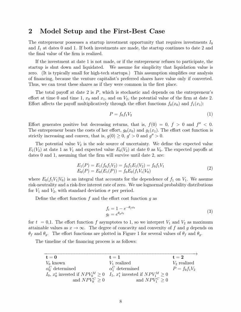
2 Model Setup and the First-Best Case

The entrepreneur possesses a startup investment opportunity that requires investments I0and I1 at dates 0 and 1. If both investments are made, the startup continues to date 2 andthe final value of the firm is realized.

If the investment at date 1 is not made, or if the entrepreneur refuses to participate, thestartup is shut down and liquidated. We assume for simplicity that liquidation value iszero. (It is typically small for high-tech startups.) This assumption simplifies our analysisof financing, because the venture capitalist’s preferred shares have value only if converted.Thus, we can treat these shares as if they were common in the first place.

The total payoff at date 2 is P , which is stochastic and depends on the entrepreneur’seffort at time 0 and time 1, x0 and x1, and on V2, the potential value of the firm at date 2.Effort affects the payoff multiplicatively through the effort functions f0(x0) and f1(x1):

P = f0f1V2 (1)

Effort generates positive but decreasing returns, that is, f(0) = 0, f > 0 and f < 0.The entrepreneur bears the costs of her effort, g0(x0) and g1(x1). The effort cost function isstrictly increasing and convex, that is, g(0) ≥ 0, g > 0 and g > 0.

The potential value V2 is the sole source of uncertainty. We define the expected valueE1(V2) at date 1 as V1 and expected value E0(V2) at date 0 as V0. The expected payoffs atdates 0 and 1, assuming that the firm will survive until date 2, are:

E1(P ) = E1(f0f1V2) = f0f1E1(V2) = f0f1V1E0(P ) = E0(E1(P )) = f0E0(f1V1|V0) (2)

where E0(f1V1|V0) is an integral that accounts for the dependence of f1 on V1. We assumerisk-neutrality and a risk-free interest rate of zero. We use lognormal probability distributionsfor V1 and V2, with standard deviation σ per period.

Define the effort function f and the effort cost function g as

ft = 1− e−θfxtgt = e

θgxt (3)

for t = 0,1. The effort function f asymptotes to 1, so we interpret V1 and V2 as maximumattainable values as x→∞. The degree of concavity and convexity of f and g depends onθf and θg. The effort functions are plotted in Figure 1 for several values of θf and θg.

The timeline of the financing process is as follows:

−−−−−−−−−−−−−−−−−−−−−−−−−−−−−−−−−−−−−−−−−−−−−−−−−−−−−−−−−−→t = 0 t = 1 t = 2V0 known V1 realized V2 realizedαC0 determined αC1 determined P = f0f1V2I0, x

∗0 invested if NPV

M0 ≥ 0 I1, x

∗1 invested if NPV

M1 ≥ 0

and NPV C0 ≥ 0 and NPV C1 ≥ 0

8

First, the entrepreneur (M ) goes to the initial venture capitalist (C ) to raise startup financ-ing. If he is willing to invest, then she and he negotiate the initial ownership shares αM0and αC0 . At date 1, V1 is observed and there is another round of bargaining over the termsof financing. If the initial venture capitalist also supplies all financing at date 1, then hecan dictate the terms and his share becomes αC1 , with a corresponding adjustment in α

M1 .

If the initial venture capitalist brings in a syndicate of new investors at date 1, then thesyndicate receives an ownership share of αS1 , and α

M1 and αC1 adjust accordingly. The terms

of financing are fixed after date 1.

2.1 First-best

In the first-best case, the entrepreneur supplies all of the money, I0 + I1, and owns the firm(αM0 = αM1 = 1). The entrepreneur maximizes NPV net of her costs of effort. If she decidesto invest, she expends the optimal efforts x0 and x1.The entrepreneur has a compound real call option. The exercise price at date 1 is

endogenous, however, because it includes the cost of effort, and effort depends on the realizedpotential value f0V1. Since we use the lognormal, our solutions will resemble the Black-Scholes formula, with extra terms capturing the cost of effort.

We now derive the first-best investment strategy, solving backwards. Details of this andsubsequent derivations are in the Appendix. By date 1, the entrepreneur’s date-0 effort andinvestment are sunk. Her date-1 NPV is

NPV M1 = max[0,maxx1(f0f1(x1)V1 − g1(x1)− I1)] (4)

The first-order condition for effort is f0V1 =g1f1, which determines optimal effort x1 and the

benefit and cost of effort, f1(x1) and g1(x1).

Define the strike value V 1 such that NPVM1 (V 1) = 0. The entrepreneur exercises her

option to invest at date 1 when V1 > V 1 and NPVM1 > 0. This strike value is similar to

the strike price of a traded option, except that the strike value has to cover the cost of theentrepreneur’s effort g1(x1) as well as the investment I1.

At date 0, the entrepreneur anticipates her choice of effort and continuation decision atdate 1. She determines the effort level x0 that maximizes NPV0, the difference between theexpected NPV at date 1 and the immediate investment I0 and cost of effort x0.

NPV M0 = max[0,maxx0(E0(NPV

M1 (x0))− g0(x0)− I0)]

E0(NPVM1 (x0)) depends on x0 in two ways. First, increasing effort at date 0 increases f0,

and thus increases the value of the startup when it is in the money at date 1. Second,increasing effort at date 0 decreases the strike value V 1 for investment at date 1 and makesit more likely that the startup will continue.

The tradeoff between effort cost and startup value is illustrated in Figure 2. The toppayoff line is the date-1 NPV for a call option with no cost of effort. In this case the valuewould be V1 and the strike price I1. The lower payoff line shows the net NPV when the

9

entrepreneur exerts less than the maximum effort at date 0 (f0 < 1). NPV1 is close to linearin V1, but the slope and the level of NPV1 are reduced by the cost of effort. We have addeda lognormal distribution to show the probability weights assigned to these NPVs. The twohorizontal lines are the date-0 financial investment I0 and the full cost I0+ g0 of investmentand effort.

We calculate E0(NPV1) by integrating from V 1(x0). Since NPVM1 (x0, V 1(x0)) = 0, the

entrepreneur’s first-order condition reduces to

E0(NPVM1 (x0)) = g0(x0).

From (4) we obtain

E0(NPVM1 (x0)) = f0

⎡⎢⎣ ∞

V 1(x0)

Π(V )V dV− 1

1 + θrθ− θr1+θr

r + θ1

1+θr

r f− θr1+θr

0

∞

V 1(x0)

Π(V )V1

1+θrdV

⎤⎥⎦(5)

where Π(V ) is the lognormal density and θr = θf/θg.

We solve for x0 analytically, using properties of the lognormal distribution. Then weevaluate NPV M0 (x0) = E0(NPV

M1 (x0))− g0 − I0. When NPV M0 (x0) > 0, the entrepreneur

invests and the firm is up and running.

Table 1 includes examples of first-best numerical results. Start with the first two linesof Panel A, which report Black-Scholes and first-best results when potential value is V0 =E0(V2) = 150 and required investments are I0, I1 = 50, 50. The standard deviation is σ = 0.4per period. The effort parameters are θf = 1.8 and θg = 0.6, so the value added by effortis high relative to the cost. Thus the option to invest in the startup should be well in themoney, even after the costs of effort are deducted.

If the costs of effort were zero, first-best NPV could be calculated from the Black-Scholesformula, with a date-1 strike price of V = 50. But when the cost of effort is introduced, Vincreases and NPV declines. First-best NPV is 37.90, less than the Black-Scholes NPV by12.13. The difference reflects the cost of effort and the increase in strike value to V = 55.35.12

Panel B repeats the example with higher standard deviation of σ = 0.8. Panels C and Dassume lower investment at date 0 and higher investment at date 1 (I0, I1 = 10, 90). NPVincreases for higher standard deviations and when more investment can be deferred. Thefirst-best initial effort decreases in these cases, though not dramatically. Panels E and Fassume θf = 0.6, so that effort is less effective, and also back-loaded investment (again, I0,I1 = 10, 90).

13 First-best effort actually increases, compared to panels C and D, but NPVdeclines dramatically.

12The effort parameters in panel A of Table 1 are θf = 1.8 and θg = 0.6. Date 0 effort is x0 = 2.4, sof0 = 0.99 and g0 = 4.59. Of course the date 0 effort is sunk by date 1. From (4), f∗1 = 0.978 and g

∗1 = 3.58.

The breakeven value level V = 55.35 is determined by 0.99× 0.978× 55.35− 3.58 = I1 = 50.13We do not include panels for equal investment (I0, I1 = 50, 50) and θf = 0.6, because NPVs are negative

in all cases where outside venture-capital financing is required. A startup with these parameters could notbe financed.

10

Figure 3 plots first-best NPV for a wide range of standard deviations and effort parame-ters. Due to exponential function choice, only θr = θf/θg, the ratio of the effort parameters,matters, so that ratio is used on the bottom-left axis. The ratio is θr = 3 in Panels A toD of Table 1 and θr = 1.0 in Panels E and F. In Figure 3, θr is varied from 1/11 to 11.The startup becomes worthwhile, with first-best NPV ≥ 0, for θr slightly below 1.0. NPVincreases rapidly for higher values of θr, then flattens out. NPV also increases with standarddeviation, especially when most investment can be deferred to date 1.

3 Monopoly financing and staged investment

Now we explore the monopoly case in which the entrepreneur approaches the venture capi-talist for financing and the initial venture capitalist can dictate terms of financing at bothdate 0 and date 1, subject to the entrepreneur’s participation constraints. The venturecapitalist will not exploit all his bargaining power, however, because of the feedback to theentrepreneur’s effort. In some cases, the venture capitalist is better off if he gives up bar-gaining power and gives the entrepreneur all the financing upfront. We do not argue thatthe monopoly case is realistic, but it is a useful benchmark, and we believe that venturecapitalists do have bargaining power, especially in early-stage financing, and receive at leastsome (quasi) rents.

By “terms of financing” we mean the fraction of common shares held by the entrepreneurand venture capitalist at dates 0 and 1. The entrepreneur’s fractional share at dates 1 and2 is αM1 , the complement of α

C1 . The entrepreneur’s share at date 0 is irrelevant in the

monopoly case, because a monopolist venture capitalist can force the terms of financing atdate 1 and is free to dilute shares awarded earlier. We do assume that the entrepreneur hasclear property rights to her shares at date 2 and that these shares cannot be taken away ordiluted between dates 1 and 2. The division of the final payoff P is enforceable once date-1financing is completed.

3.1 Effort and investment at date 1.

Both the entrepreneur and the venture capitalist now have the option to participate at date1. There are two derivative claims on one underlying asset. Both must be exercised in orderfor the project to proceed.

At date 1 the entrepreneur decides whether to exercise her option to continue, based onher strike price, the cost of optimal effort g1(x1). But first the venture capitalist sets α

C1 and

αM1 = 1−αC1 and decides whether to put up the financial investment I1. We can focus on theventure capitalist’s decision if we incorporate the entrepreneur’s response into the venturecapitalist’s optimization problem.

The equation for the entrepreneur’s NPV is similar to Eq. (4), except that the second-period investment I1 drops out and firm value is multiplied by the entrepreneur’s shareαM1 .

NPV M1 (αC1 ) = max[0,maxx1

(αM1 f0f1(x1)V1 − g1(x1))] (6)

11

The maximum share the venture capitalist can take is obtained by setting NPV M1 (αC1 ) = 0.

This defines αC1 (max) and αM1 (min). When αM1 (min) ≥ αM1 , the entrepreneur will notparticipate.14 The venture capitalist chooses αC1 to maximize his date-1 NPV, subject tohis and the entrepreneur’s participation constraints.

NPV C1 = max

⎡⎣0, maxαC1 ∈(0,αC1 (max)]

αC1 f0f1(x1)V1−I1⎤⎦ (7)

If the entrepreneur’s participation constraint is binding, the venture capitalist assigns

αC1 (max). Otherwise, he assigns an interior value. But in most of our experiments, VC1 , the

venture capitalist’s strike value for the monopoly case, falls in the region αC1 ∈ 0,αC1 (max)where the entrepreneur’s NPV is positive. In these cases the venture capitalist is better offby taking a share αC1 < αC1 (max) in order to give the entrepreneur stronger incentives. Nev-ertheless, those incentives are weaker than first-best, because αM1 (x0) < 1, which decreasesthe expected payoff by reducing x1.

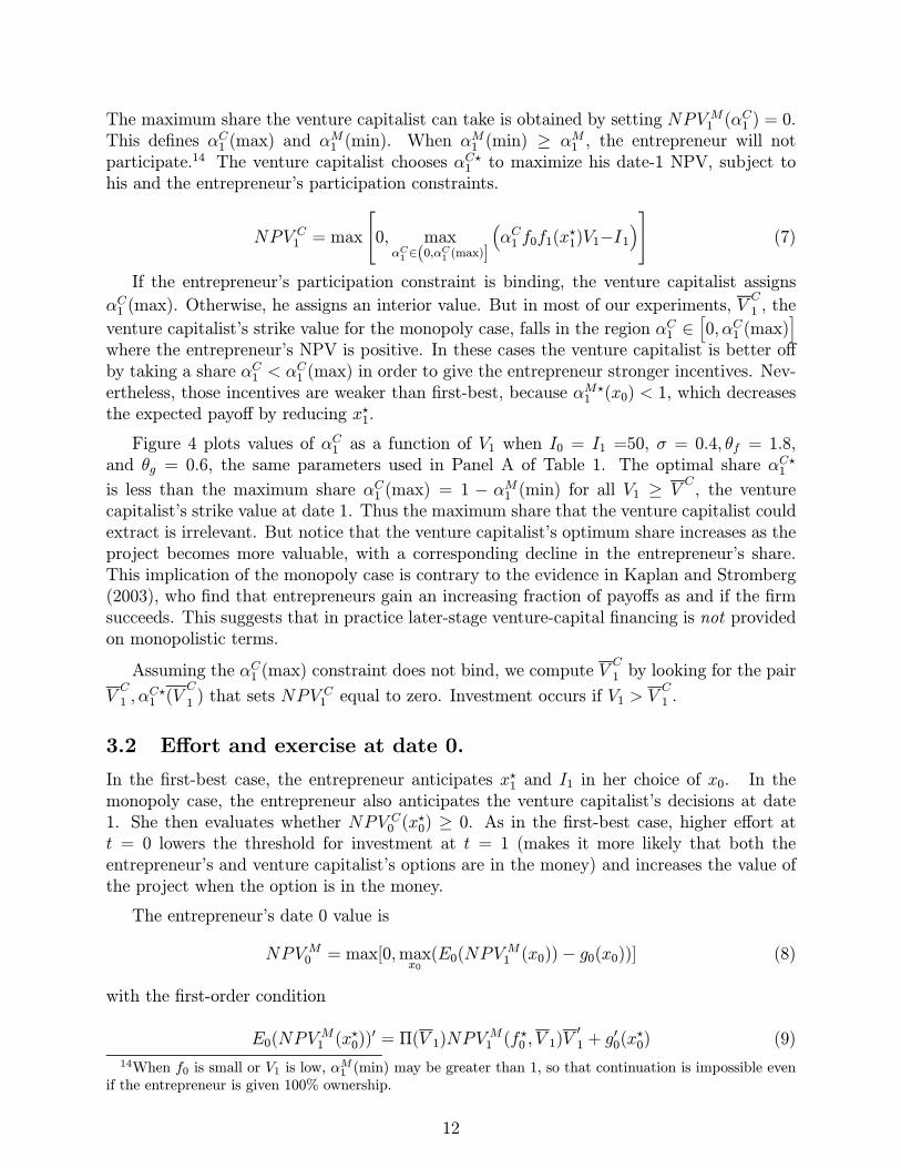
Figure 4 plots values of αC1 as a function of V1 when I0 = I1 =50, σ = 0.4, θf = 1.8,and θg = 0.6, the same parameters used in Panel A of Table 1. The optimal share αC1is less than the maximum share αC1 (max) = 1 − αM1 (min) for all V1 ≥ V

C, the venture

capitalist’s strike value at date 1. Thus the maximum share that the venture capitalist couldextract is irrelevant. But notice that the venture capitalist’s optimum share increases as theproject becomes more valuable, with a corresponding decline in the entrepreneur’s share.This implication of the monopoly case is contrary to the evidence in Kaplan and Stromberg(2003), who find that entrepreneurs gain an increasing fraction of payoffs as and if the firmsucceeds. This suggests that in practice later-stage venture-capital financing is not providedon monopolistic terms.

Assuming the αC1 (max) constraint does not bind, we compute VC1 by looking for the pair

VC1 ,α

C1 (V

C

1 ) that sets NPVC1 equal to zero. Investment occurs if V1 > V

C1 .

3.2 Effort and exercise at date 0.

In the first-best case, the entrepreneur anticipates x1 and I1 in her choice of x0. In themonopoly case, the entrepreneur also anticipates the venture capitalist’s decisions at date1. She then evaluates whether NPV C0 (x0) ≥ 0. As in the first-best case, higher effort att = 0 lowers the threshold for investment at t = 1 (makes it more likely that both theentrepreneur’s and venture capitalist’s options are in the money) and increases the value ofthe project when the option is in the money.

The entrepreneur’s date 0 value is

NPV M0 = max[0,maxx0(E0(NPV

M1 (x0))− g0(x0))] (8)

with the first-order condition

E0(NPVM1 (x0)) = Π(V 1)NPV

M1 (f0 , V 1)V 1 + g0(x0) (9)

14When f0 is small or V1 is low, αM1 (min) may be greater than 1, so that continuation is impossible even

if the entrepreneur is given 100% ownership.

12

Here there are no closed-form expressions. We solve the first-order condition and de-termine x∗0 numerically. Given x

∗0, and assuming that the entrepreneur wants to go ahead

(NPV M0 (x∗0) > 0), the venture capitalist invests if:

NPV C0 = max[0, E0(NPVC1 (x0))− I0] > 0 (10)

Thus two options must be exercised at date 0 in order to launch the startup. Theentrepreneur picks x∗0 to maximize the value of her option to continue at date 1, and thendetermines whether this value exceeds her current strike price, the immediate cost of effortg∗0. The venture capitalist values his option to invest I1 at date 1, taking the entrepreneur’simmediate and future effort into account, and then decides whether to invest I0.

Monopoly financing can be extremely inefficient. The venture capitalist’s ability to claima large ownership fraction at date 1 reduces the entrepreneur’s effort at date 0 as well as date

1, reducing value and increasing the venture capitalist’s breakeven point VC1 . For example,

compare the monopoly and first-best results in Panel A of Table 1. The entrepreneur’s

initial effort falls by about 50 percent from the first-best level and the date-1 strike value VC1

increases by almost 30 percent. The entrepreneur’s NPV drops by more than 90 percent.Overall NPV drops by more than half. Similar value losses occur in panels B to F. In PanelE, a startup with first-best NPV of 10.98 cannot be financed in the monopoly case. NPVwould be negative for both the entrepreneur and the initial venture capitalist.

3.3 Monopoly financing without staged investment

The incentive problems of the monopoly case can sometimes overwhelm the option-like ad-vantages of staged financing. All may be better off if the entire investment I0+ I1 is givento the entrepreneur upfront and she is granted full control thereafter.

In the monopoly, no-staging case, the entrepreneur and venture capitalist bargain onlyonce at date 0 to determine their ownership shares αM and αC , which are then fixed fordates 1 and 2. The entrepreneur calculates her NPV at date 1 just as in the monopolycase with staging, but her share of the firm αM1 is predetermined. Also, she ignores thefinancial investment I1 and continues at date 1 so long as her NPV exceeds her cost of effort,g1(x1).

15 The venture capitalist retains monopoly power over financing at date 0, but losesall his bargaining power at date 1. He sets αC to maximize his NPV at date 0, taking intoaccount the effects on the entrepreneur’s effort at dates 0 and 1. His maximization problemis identical in appearance to Eq. (10) but the values of x∗0, x

∗1 and α

C1 = αC0 are different. The

entrepreneur’s date-0 maximization problem closely resembles Eq. (8) except for the choicesof x∗1 and α

C1 = αC0 . If both parties’ participation constraints are met at date 0 (NPV

C0 ≥ 0

and NPV M0 ≥ 0), the startup is launched.The value loss from the holdup problem in the monopoly, staged financing case can be

so severe that it can actually exceed the cost of inefficient continuation in the no-stagingcase. For example, note the improvement in the no-staging case in Panel A of Table 1. The

15We do assume that the entrepreneur cannot launch the firm at date 0 and then run off with the date-1investment I1. Venture-capital investors typically hold convertible preferred shares and have priority inliquidation.

13

NPV to the entrepreneur more than doubles, compared to the monopoly case with stagedinvestment, and overall NPV increases from 16.47 to 26.89.

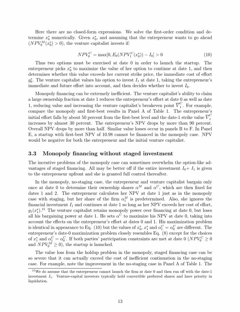
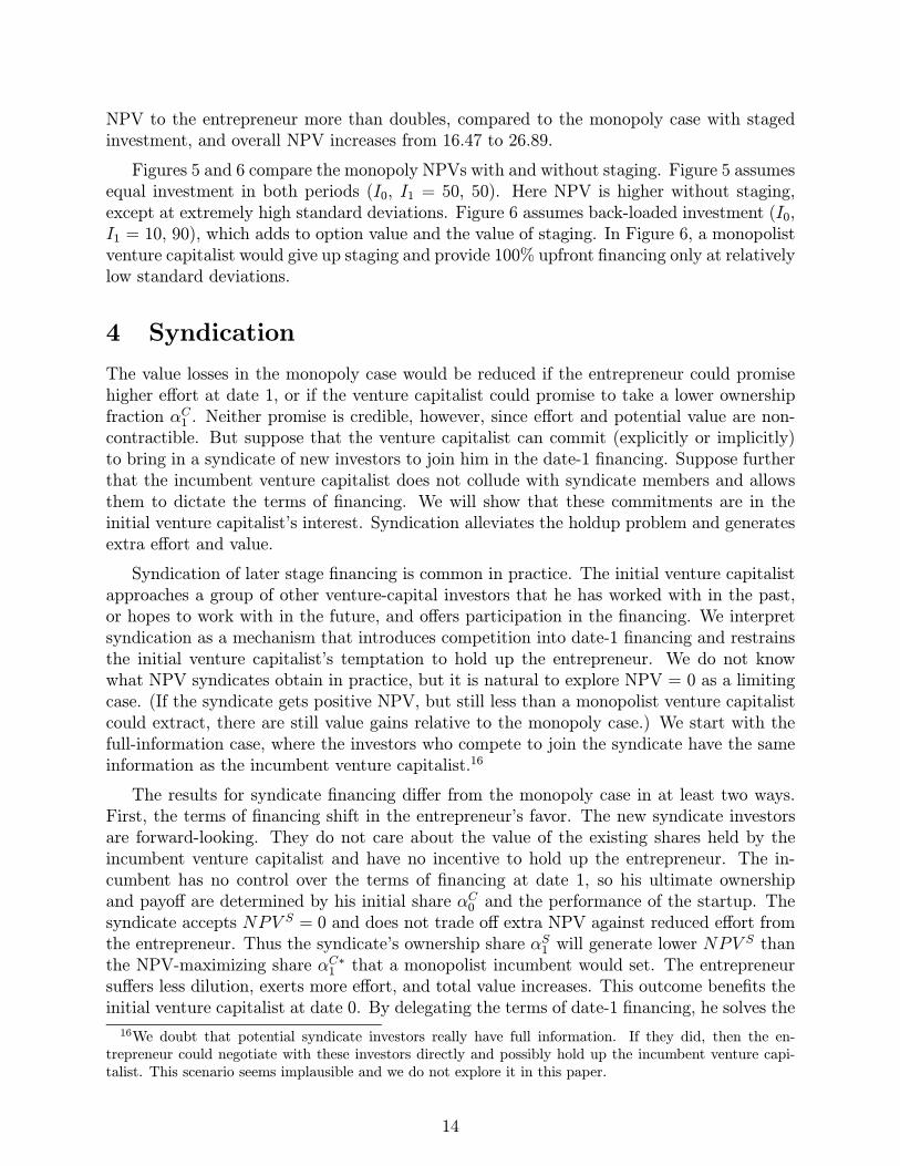
Figures 5 and 6 compare the monopoly NPVs with and without staging. Figure 5 assumesequal investment in both periods (I0, I1 = 50, 50). Here NPV is higher without staging,except at extremely high standard deviations. Figure 6 assumes back-loaded investment (I0,I1 = 10, 90), which adds to option value and the value of staging. In Figure 6, a monopolistventure capitalist would give up staging and provide 100% upfront financing only at relativelylow standard deviations.

4 Syndication

The value losses in the monopoly case would be reduced if the entrepreneur could promisehigher effort at date 1, or if the venture capitalist could promise to take a lower ownershipfraction αC1 . Neither promise is credible, however, since effort and potential value are non-contractible. But suppose that the venture capitalist can commit (explicitly or implicitly)to bring in a syndicate of new investors to join him in the date-1 financing. Suppose furtherthat the incumbent venture capitalist does not collude with syndicate members and allowsthem to dictate the terms of financing. We will show that these commitments are in theinitial venture capitalist’s interest. Syndication alleviates the holdup problem and generatesextra effort and value.

Syndication of later stage financing is common in practice. The initial venture capitalistapproaches a group of other venture-capital investors that he has worked with in the past,or hopes to work with in the future, and offers participation in the financing. We interpretsyndication as a mechanism that introduces competition into date-1 financing and restrainsthe initial venture capitalist’s temptation to hold up the entrepreneur. We do not knowwhat NPV syndicates obtain in practice, but it is natural to explore NPV = 0 as a limitingcase. (If the syndicate gets positive NPV, but still less than a monopolist venture capitalistcould extract, there are still value gains relative to the monopoly case.) We start with thefull-information case, where the investors who compete to join the syndicate have the sameinformation as the incumbent venture capitalist.16

The results for syndicate financing differ from the monopoly case in at least two ways.First, the terms of financing shift in the entrepreneur’s favor. The new syndicate investorsare forward-looking. They do not care about the value of the existing shares held by theincumbent venture capitalist and have no incentive to hold up the entrepreneur. The in-cumbent has no control over the terms of financing at date 1, so his ultimate ownershipand payoff are determined by his initial share αC0 and the performance of the startup. Thesyndicate accepts NPV S = 0 and does not trade off extra NPV against reduced effort fromthe entrepreneur. Thus the syndicate’s ownership share αS1 will generate lower NPV

S thanthe NPV-maximizing share αC∗1 that a monopolist incumbent would set. The entrepreneursuffers less dilution, exerts more effort, and total value increases. This outcome benefits theinitial venture capitalist at date 0. By delegating the terms of date-1 financing, he solves the

16We doubt that potential syndicate investors really have full information. If they did, then the en-trepreneur could negotiate with these investors directly and possibly hold up the incumbent venture capi-talist. This scenario seems implausible and we do not explore it in this paper.

14

incomplete contracting problem that causes the holdup problem in the monopoly case withstaged financing.

Second, under zero-NPV date-1 financing, the initial venture capitalist effectively owns acall option with a zero exercise price and will always want the investment to proceed at date1 whether or not the project can generate enough value to cover the syndicate’s investment.With full information, it does not matter whether the initial venture capitalist participates inthe syndicate, because the syndicate’s investment is zero-NPV. Of course the initial venturecapitalist’s participation matters if the syndication terms are not fully competitive. Thehigher the NPV for the syndicate, the closer is the syndicate case to the monopoly case.

4.1 Effort and investment at date 1

For a given share αM1 , the entrepreneur’s NPV and maximization problem at date 1 are thesame as in the monopoly case. We obtain x1, f1 , g1, and NPV

M1 (α

S1 ) exactly as in Eq. (6),

but with αM1 = αM0 (1−αS1 ). The share given to the outside syndicate, αS1 , is determined byNPV S1 = 0, that is, by I1 = αS1 f0f1(x1)V1. Investment at date 1 occurs for V1 > V

S1 . We

solve for VS1 by finding the value of α

S1 that maximizes NPV1, subject to the constraint that

NPV S = 0 for the syndicate. The solution is generally in the region where NPV M1 (αS1 ) > 0

at V 1 and αM1 < αM1 (min).

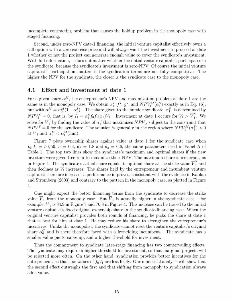
Figure 7 plots ownership shares against value at date 1 for the syndicate case whenI0, I1 = 50, 50, σ = 0.4, θf = 1.8 and θg = 0.6, the same parameters used in Panel A ofTable 1. The top two lines show the syndicate’s maximum and optimal shares if the newinvestors were given free rein to maximize their NPV. The maximum share is irrelevant, as

in Figure 4. The syndicate’s actual share equals its optimal share at the strike value VS1 and

then declines as V1 increases. The shares held by the entrepreneur and incumbent venturecapitalist therefore increase as performance improves, consistent with the evidence in Kaplanand Stromberg (2003) and contrary to the pattern in the monopoly case, as plotted in Figure4.

One might expect the better financing terms from the syndicate to decrease the strikevalue V 1 from the monopoly case. But V 1 is actually higher in the syndicate case — forexample, V 1 is 84.9 in Figure 7 and 70.8 in Figure 4. This increase can be traced to the initialventure capitalist’s fixed original ownership share in the syndicate-financing case. When theoriginal venture capitalist provides both rounds of financing, he picks the share at date 1that is best for him at date 1. He may reduce his share to strengthen the entrepreneur’sincentives. Unlike the monopolist, the syndicate cannot reset the venture capitalist’s originalshare αC0 and is there therefore faced with a free-riding incumbent. The syndicate has asmaller value pie to carve up, and a higher threshold for investment.

Thus the commitment to syndicate later-stage financing has two countervailing effects.The syndicate may require a higher threshold for investment, so that marginal projects willbe rejected more often. On the other hand, syndication provides better incentives for theentrepreneur, so that low values of f0V1 are less likely. Our numerical analysis will show thatthe second effect outweighs the first and that shifting from monopoly to syndication alwaysadds value.

15

4.2 Renegotiation at date 1

Of course a low realization of V1 could trigger a renegotiation between the incumbent and theentrepreneur to reset the incumbent’s initial share αC0 before syndicate financing is sought.The incumbent can transfer ownership to the entrepreneur, retaining αC(R) < αC∗0 , whereαC(R) denotes the incumbent’s renegotiated equity stake. The incumbent may be betteroff accepting a reduced ownership share to improve the chance of success for low values

of V1 or to increase continuation for V1 < VS1 . By accepting a lower ownership share, the

incumbent improves effort incentives for the entrepreneur to the point where enough extravalue is added to support syndicate financing at NPV = 0. Of course the incumbent willgive up as little as possible. In the worst renegotiation case, where V1 approaches a lowerbound, the value of the incumbent’s shares approaches zero, just as in the monopoly case.

Renegotiation requires dilution of the incumbent venture capitalist’s ownership share.Dilution could happen in several ways. For example, the incumbent could provide bridgefinancing on terms favorable to the entrepreneur. Dilution could also occur in a ”downround” — a round of financing where new investors buy in at a price per share lower than inprevious rounds. But our model says that a down round should dilute the entrepreneur lessthan the incumbent venture capitalist. The entrepreneur could be given additional sharesor options, for example.

While renegotiation adds value ex post by improving effort and preserving access tofinancing, the flexibility to reset shares at date 1 could introduce new problems. Supposethe initial venture capitalist sets αC0 at a very high level, knowing that he can renegotiatedown to the monopoly level at date 1, even when the realized value V1 exceeds the syndicate

strike value VS1 .17 The entrepreneur would then cut back effort at dates 0 and 1 and reduce

the value of the firm. This strategy amounts to a return to monopoly financing. It wouldreduce date-0 value to the venture capitalist as well as the entrepreneur.

Thus two conditions must hold in order for syndicate financing to work as we havedescribed it. First, the initial venture capitalist has to commit at date 0 to syndicate atdate 1. In practice this is not an explicit, formal commitment, but syndication is standardoperating procedure. As part of the commitment, the initial venture capitalist has to limithis initial ownership share αC0 to its level in the syndicate case, so that he cannot start with ahigher value and bargain down to the monopoly share αC∗1 at date 1. The commitment is inthe venture capitalist’s interest, because it increases his ex ante value relative to the monopolycase. Second, the terms of financing in later rounds should be reasonably competitive. Inpractice they may not be perfectly competitive, but we believe the terms are materiallybetter for the entrepreneur than the monopoly terms would be.

It turns out that opportunities for renegotiation are rare in our numerical experimentsfor the syndicate case. Therefore, incorporating the benefits of renegotiation would addrelatively little to NPV at date 0. For example, including renegotiation gains would increasethe NPVs reported in Table 1 by about 2% of the required total investment of I0+I1 = 100.

18

17The entrepreneur could retain the upside if she could bypass the incumbent venture capitalist and godirectly to the syndicate for financing. In practice the incumbent could block this end run by refusing toparticipate in the syndicate. The syndicate would assume that the incumbent has inside information, andwould interpret the refusal to participate as bad news sufficient to deter their investment.18We approximate renegotiation gains (holding αC∗0 and x0 constant) by solving for (1) the value realization

16

4.3 Effort and exercise at date 0

At date 0, the venture capitalist sets αC0 and the entrepreneur decides how much effort toexert. Given αC0 , the entrepreneur chooses x0 to maximize:

NPV M0 (αC0 ) = max[0,maxx0

(E0(NPVM1 (x0(α

C0 ),α

C0 )− g0(x0(αC0 )))] (11)

The entrepreneur anticipates the syndicate’s share αS1 as a function of date-1 value V1. Fora given αC0 , date-1 syndicate financing will result in less dilution of her share than in themonopoly case, so she provides higher effort at t = 0 as well as at t = 1. We cannot expressNPV or effort in closed form, so we compute them numerically.

The venture capitalist anticipates the entrepreneur’s reaction when he sets αC0 . He must

restrict his search to αC0 ∈ 0,αC0 (max) , where αC0 (max) is determined by

E0(NPVM1 (x0(α

C0 (max)),α

C0 (max))− g0(x0(αC0 (max)))) = 0 (12)

This constraint rarely binds, since at the margin there is almost always value added byleaving positive value to the entrepreneur. Thus αC∗0 is determined by

αC0 = arg maxαC0 ∈(0,αC0 (max)]

E0(NPVC1 (x0(α

C0 ),α

C0 ))− I0 (13)

If NPV C0 ≥ 0, investment proceeds.Typical results for syndicate financing are shown in Table 1. Effort and value increase

across the board, despite increases in the strike value VS

1 from the monopoly case. We findthat syndicate financing dominates monopoly financing with or without staged financing.Syndicate financing is better ex ante for the initial venture capitalist and also increases overallNPV. This is true for all parameter values, including values outside the range reported inTable 1. Yet there are still value losses relative to the first best.

4.4 The fully competitive case

Of course first best is never attainable when the entrepreneur has to seek outside financing.Table 1 shows an alternative benchmark, the fully competitive case, in which all venturecapital investors, including the initial investor at date 1, receive NPV = 0. Fully competitivefinancing gives an upper bound on the overall NPV when the entrepreneur has no moneyand has to share her marginal value added with outside investors. Solution procedures forthe fully competitive case are identical to the syndication case, except that αC0 is set so thatNPV C0 = 0.

Figure 8 shows date-1 ownership shares for the fully competitive case in the same formatas the syndication case in Figure 7. Two things stand out. First, the entrepreneur’s share

at which the venture capitalist will start to reduce his share; (2) the new strike value and (3) the integralof NPV changes over this range. Only a small portion of the renegotiation gains come from more efficient

continuation decisions (VS

1 (R) < V1 < VS

1 ). Most of the gains can be attributed to better effort incentives

(higher x1) in the region where the project continues regardless (V1 > VS1 ). These gains further increase the

value advantages of syndicate financing over monopoly financing.

17

is higher and the initial venture capitalist’s lower than in Figure 7, because competitivefinancing at date 0 gives relatively more shares to the entrepreneur. Both shares of courseincrease with the realized value V1. Second, the strike value V 1 is lower in the competitivecase, primarily because the entrepreneur’s initial effort is higher. Note also that the fullycompetitive NPVs, which go entirely to the entrepreneur, are less than in the first-bestcase, because the entrepreneur’s effort is lower. There is always some value loss when theentrepreneur has to share the marginal value added by her effort with outside investors.

4.5 Syndication with asymmetric information

So far we have assumed that the incoming syndicate investors and the incumbent venturecapitalist are equally informed. Now we consider asymmetric information between the in-cumbent and new investors.

Both the incumbent and entrepreneur want the syndicate to perceive a high value V1.The more optimistic the syndicate, the higher the ownership shares retained by the incum-bent and entrepreneur. Reducing the syndicate’s share also increases the entrepreneur’seffort. Therefore, mere announcements of “great progress” or “high value” coming from theentrepreneur or incumbent are not credible.

Credibility may come from the incumbent’s fractional participation in date-1 financing.Suppose the incumbent invests βI1 and the outside syndicate the rest. What participationfraction β is consistent with truthful revelation of V1? If we could hold the entrepreneur’seffort constant, we could rely on Admati and Pfleiderer’s (1994) proof that β should be fixedat the incumbent investor’s ownership share at date 0, that is, at αC0 . This fixed-fractionrule would remove any incentive for the incumbent to over-report V1. (The more he over-reports, the more he has to overpay for his new shares. When β = αC0 , the amount overpaidcancels out any gain in the value of his existing shares.)19 The fixed-fraction rule would alsoinsure optimal investment, since the incumbent’s share of date-1 investment exactly equalshis share of the final payoff V2. Admati and Pfleiderer also show that no other financing ruleor procedure works in their setting.

Fixed-fraction financing does not induce truthful information revelation in our model,although a modified fixed-fraction financing works in some cases. The problem is the effectof the terms of date-1 financing on the entrepreneur’s effort. Suppose the incumbent investortakes a fraction β = αC0 of date-1 financing and then reports a value V1 that is higher than thetrue value V1. If the report is credible, the new shares are over-priced. The incumbent doesnot gain or lose from the mispricing, because β = αC0 , but the entrepreneur gains on his oldshares at the syndicate’s expense. Since the entrepreneur’s ownership share is higher than itwould be under a truthful report, she exerts more effort, firm value increases, and both theentrepreneur and incumbent are better off. Therefore the incumbent will over-report.

A modified fixed-fraction rule can work, however, provided that β is set above αC0 andeffort is not too sensitive to changes in the entrepreneur’s NPV at date 1. The requireddifference between β and αC0 depends on the responsiveness of the entrepreneur’s effort to

19The fixed-fraction rule would also remove any incentive to underreport. The more the incumbent under-reports, the more he gains on the new shares. But the amount of profit made on the new shares is exactlyoffset by losses incurred on existing shares.

18

her ownership share. In many cases, a constant β set a few percentage points above αC0removes the incentive to overreport over a wide range of V1 realizations. But this rule maybreak down as a general revelation mechanism in at least three ways.

First, when V1 is very low but exceeds V 1, we find situations where the required β exceeds1. This would make sense only if the new syndicate investors could short the company, sowe must constrain β < 1. This outcome is common in our numerical results, because theincumbent’s initial share αC0 is frequently above 85% - 90%, and in some of these cases theentrepreneur’s effort is very sensitive to the value of her stake in the firm. There is notmuch room for β to increase between these starting points and a maximum level strictly lessthan 1. When β hits the maximum, the modified fixed fraction rule fails to induce truthfulrevelation.20

Second, the modified fixed fraction rule also fails when V1 falls just below V 1. In this casethe incumbent’s incentive to over-report becomes very strong, and only extremely high βscan discipline the incumbent to tell the truth. This problem flows from the discontinuity ofthe entrepreneur’s effort at the strike value V 1. Here the limit of β as V1 approaches V 1 frombelow is infinity and no fixed-fraction rule works. This problem can be solved, however, if theincumbent and the entrepreneur renegotiate their ownership shares when V1 falls between

the monopoly and syndicate strike values VC1 and V

S1 . If the incumbent venture capitalist

renegotiates, the lower strike value removes the discontinuity of effort. As the incumbent’sshare declines, it is easier to find a β < 1 that works. The required β approaches 0 as V1approaches V

C1 and the incumbent’s share approaches zero.

The third problem arises at high levels of V1. Setting β > αC0 gives the incumbentventure capitalist an incentive to under-report V1. The incumbent would gain more fromunderpricing the new shares and buying them cheaply than he would lose from dilution ofhis existing stake. Revelation works only if this incentive is offset by the impact on theentrepreneur’s effort. But as V1 and V1 increase, effort becomes higher and less sensitive tothe terms of financing. As effort tops out, the incentive to under-report takes over. Thiscould be prevented locally by allowing β to decrease with V1, returning to β = αC0 at very highvalues. But then the almost-fixed fraction rule fails globally to induce truthful informationrevelation, because at lower V1 realizations he wants to over-report to these higher levels atwhich β = αC0 .

One possible solution, not fully explored here, is to introduce more complex contractsthat allow signalling along two dimensions. For example, the incentive for the incumbentventure capitalist to under-report at high levels of V1 could be offset by an incentive contractthat grants the entrepreneur extra shares if the incumbent reports very high project value.With this additional provision in place, it should be possible to allow β to decrease with V1,reaching β = αC0 at high values of V1. This could be one justification for contingent shareawards to the entrepreneurs, as observed in Kaplan and Stromberg (2003). Alternatively,the entrepreneur could be granted a series of stock options with increasing exercise prices,so that the entrepreneur’s final ownership share increases at high values of V2.

20This failure is less frequent if the entrepreneur has some personal wealth and can co-invest with theventure capitalist at date 0. The coinvestment reduces the venture capitalist’s ownership share and providesmore room for β to increase to a maximum level strictly less than 1.

19

When the modified fixed fraction rule fails, the syndicate investors face the asymmetricinformation problem analyzed by Myers and Majluf (1984). In the special case of their modelthat is closest to our problem here, the firm has no assets in place (no value in liquidation),so it goes ahead with financing on terms fixed by the new investors’ knowledge of the averagevalue of V1. Syndicate investors would have to infer the average V1 from conditions at date0, the entrepreneur’s effort functions and the entrepreneur’s and incumbent’s decision rules,given the anticipated terms of date-1 financing. But the investors do not know the truevalue V1, so their new financing is overpriced when V1 is low and underpriced when V1 ishigh. This leads to more effort when V1 is low and less when it is high, compared to thefull-revelation case. But again there are problems. For example, if V1 is high, the incumbentwill be better off cancelling syndicate financing and providing the date-1 money directly.But if this is allowed, then the incumbent will have an incentive to claim a high value V1 inorder to reclaim monopoly power over the terms of financing. In addition, if the syndicateinvestors know less than the incumbent and the incumbent is free to finance the investmentfrom his own pocket, then the incumbent will only raise syndicate financing if the syndicateis paying too much. Therefore a rational syndicate will not invest.21

Even if the revelation mechanism fails, there may be other ways to convey V1. Thevalue of the incumbent investor’s reputation could generate truthful reports in a repeatedgame setting, for example. The syndicate usually includes other venture capitalists that theincumbent has worked with in the past and expects to work with in the future.

5 Summary of Numerical Results

Table 1 illustrates our main results. It shows surprisingly large value losses in most cases,relative to first-best. (For now ignore the debt-financing entries.) Value losses are greatestin the monopoly case where the initial venture capitalist provides all financing and dictatesthe terms of financing at date 1 as well as date 0. This does not imply that the venturecapitalist extracts all value, leaving the entrepreneur with zero NPV. The venture capitalistwants to preserve the entrepreneur’s incentives to some extent. Nevertheless, the financingterms that maximize value for the venture capitalist usually leave the entrepreneur with asmall minority slice of a diminished pie.

The problem with staged financing is that a monopolistic venture capitalist cannot com-mit not to hold up the entrepreneur ex post. Thus NPV can be higher and the initial venturecapitalist better off if staged financing is abandoned and all financing is committed at date0. Complete upfront financing is superior for all effort parameters (all values of θr = θf/θg)when option value is relatively low, as it is for most of the range of standard deviationsin Figure 5. Figure 6 shows that when the option value is high, staged financing is moreefficient, despite the monopoly holdup problem.

Syndication of date-1 financing always makes both the entrepreneur and the initial ven-ture capitalist better off as long as the syndicate’s financing terms are reasonably competi-tive. This key result of our paper is evident in Table 1 and also holds generally. We believethat our syndicate case, in which the initial venture capitalist can set financing terms atdate 0 but not date 1, is a good match to actual venture capital contracting. Of course we

21This is a variation of Myers and Majluf’s (1984) pecking-order proofs.

20

observe syndication in practice, but that observation does not settle whether the terms ofsyndicate financing are competitive (NPV = 0) or monopolistic. Our analysis indicates thatsyndication terms are reasonably competitive. With monopoly financing terms at date 1,we find that the entrepreneur’s final ownership share is a decreasing function of firm value.With competitive terms, as in our syndication case, the entrepreneur’s share is an increasingfunction of value, consistent with practice (Kaplan and Stromberg (2003)).

The syndicate case is still inefficient, because it gives the initial venture capitalist thebargaining power to set financing terms at date 0. We believe that venture capitalists do havebargaining power and receive at least some (quasi) rents in early financing rounds. They havebargaining power because of experience and expertise, because of the fixed costs of setting upa venture capital partnership and because of the cost and delay that the entrepreneur wouldabsorb in looking for another venture-capital investor. But there are obviously efficiencyimprovements if and as the terms of date-0 financing become more competitive. The fullycompetitive case shows the limit where the initial venture capitalist has no special bargainingpower and just receives NPV = 0. Even the fully competitive case falls short of first best,however. The entrepreneur’s effort falls whenever outside financing has to be raised, becausethe entrepreneur bears the full cost of effort, but has to share the marginal value added byeffort with the outside investors.

Figure 9 summarizes value losses for the monopoly, no-staging, syndication and fullycompetitive cases over a wide range of the effort parameter θr. Value loss is defined as thedifference between NPV at date 0 and first-best NPV. The four panels correspond to panelsA to D in Figure 1, except for the variation in θr. Figure 10 repeats Figure 9 for a moreprofitable startup with V0 = 200.

The value losses plotted in Figure 9 increase rapidly with θr when θr is below 1.0, butthe losses are always less in the syndication case than in the monopoly cases. The lossesin the syndicate case still appear economically significant, however. The only situations inwhich losses do not appear significant occur in the fully competitive case when θr is above2.0. High values for θr mean that effort generates value at relatively little cost, so that theentrepreneur is willing to expend close to first-best effort in the fully competitive case, eventhough the marginal benefit of effort is shared with outside investors.

Value losses in the monopoly, no staging case increase as standard deviation is increasedfrom σ = 0.4 to 0.8. This is as expected, since staged financing is more valuable as volatilityincreases. But value losses may also increase with standard deviation in the monopoly andsyndication cases, at least for the region where θr is about 1.0 and higher. We found this sur-prising. Our original intuition was that increased uncertainty would enhance the optionalityof investment and mitigate incentive problems. Instead it can make these problems worse,because more uncertainty can lead to lower initial effort.22 Compare the bottom-left andbottom-right panels in Figure 9, for example. The effects of volatility on effort and valuecan also be seen in panels E and F of Table 1. In the syndicate case, the value loss in panel

22When overall NPV is near zero, the entrepreneur’s effort x0 increases rapidly with σ. The more un-certainty, the greater chance that the entrepreneur’s call option will be in the money and the greater themarginal reward to effort. But as θr increases and NPV rises, effort eventually declines as σ increases,because the marginal impact of effort is less. The difference can be traced to the slope of the cumulativelognormal, which is lower at the mean when σ is high.

21

E, with σ = 0.4, is 10.98 - 1.55 = 9.43. In panel F, with σ = 0.8, value loss is 27.72 - 17.50= 10.22. Initial effort falls from x0 = 3.05 in panel E to x0 = 2.80 in panel F.

The value-loss patterns in Figure 9 are repeated in Figure 10, where V0 = 200 ratherthan 150. Financing is feasible in Figure 10 at lower levels of the effort parameter θr. Valuelosses are lower for the fully competitive case, but actually increase for the monopoly andsyndication cases. This problem can be traced to the initial venture capitalist’s bargainingpower at date 0. Consider the monopoly case. Since the marginal product of effort is higherwhen V0 = 200, the entrepreneur will put in more effort at date 1. This allows the initialventure capitalist to tighten the screws and extract a greater ownership share, which in turnfeeds back to lower effort by the entrepreneur at date 0.

The effects of other parameters on our results are generally as expected. NPV increaseswhen the ratio θr = θf/θg increases. The strike value V falls with θr, increasing the proba-bility that the date-1 option to invest is in the money, and when the option is in the moneyit is worth more. Overall NPV increases when σ increases (generating more uncertainty inV1 and V2) and when a greater fraction of investment can be deferred to date 1. These effectsare natural for investments in real options.

6 Debt financing

So far we have considered only equity financing, following venture-capital practice. Is equityfinancing efficient for venture capitalists? We cannot answer this question without derivingoptimal contracts, a task that we do not attempt in this paper. But it is interesting toconsider the alternative of debt financing. We have interpreted syndicate financing as adevice to secure the entrepreneur’s effort by protecting her from ex-post holdup. Could aswitch to debt financing achieve the same or better result? In traditional agency models,debt financing calls forth maximum effort, because the entrepreneur retains the maximumfraction of the value added at the margin by her effort. Perhaps we have oversimplifiedventure-capital practice to the extent that debt dominates equity as a financing contract.

In this section we show that debt is not superior to equity. When effort and investmentare made in stages, debt financing can actually amplify the hold-up problem and reducethe entrepreneur’s initial effort at date 0. We will show that debt financing could increaseefficiency in some cases, however.

Suppose that the startup firm issues debt rather than equity to venture-capital investors.The face value of the debt equals the required investment. Of course, this debt faces a highprobability of default, so the promised payoff at date 2, including interest, is well above facevalue. (Safe debt is nearly impossible, given the high variance of most startups and mostentrepreneurs’ limited funds available for equity investment.) The promised debt payoff(face value plus interest) sets a strike value for V2 below which the startup defaults and theinvestors receive all of the startup’s payoff P . Above this point the investors’ payoff is cappedand the entrepreneur receives the residual. Thus debt financing converts the entrepreneur’sstake to a call option, and our discussion of debt financing also applies if the entrepreneurreceives no shares but only options. The implicit call options created by debt financingwould probably be out of the money, however, because the promised payment to the venture

22

capitalists would have to exceed total investment by enough to cover the risk of failure anddefault.

Now we revisit the monopoly case, holding all aspects of our model constant, except thatat date 1 the venture capitalist and entrepreneur negotiate a promised debt payoffK1 insteadof ownership shares αC1 and α

M1 . (With debt, α

M1 = 1.) The entrepreneur’s NPV at date 1

is her expected residual payout at date 2, that is, E0[max(0, f0f1V2 −K1)]. As before, theentrepreneur chooses effort to maximize NPV M1 , and the venture capitalist chooses K

∗1 to

maximize NPV C1 . The startup continues if NPVC1 > I1. At date 0, the entrepreneur antic-

ipates K∗1 and chooses initial effort accordingly. We solve numerically for the entrepreneur’seffort, the promised payoff K∗1 and the venture capitalist’s and entrepreneur’s NPVs. If bothparties’ participation constraints are met at date 0, the venture is launched.

Table 1 shows examples comparing debt versus equity financing in the monopoly case.It is immediately clear that debt is no panacea. When monopoly debt financing is feasible,it can enhance effort and NPV. In Panels B and D of Table 1, for example, initial effort ishigher and NPVs increase in the monopoly (debt) cases. The resulting NPVs in these casesapproach the fully competitive outcome. But in Panels A, C and F startups that could befinanced by a monopolist venture capitalist with equity cannot be financed with debt. Thisbreakdown occurs because debt makes the holdup problem worse. At date 1, the venturecapitalist is able to set the promised debt payoff so high that the entrepreneur is left withwith a very small slice of value. The entrepreneur’s effort at date 1 is increased, given K∗1 ,because the entrepreneur holds an option and receives all value in excess of K∗1 . But theentrepreneur’s date-1 NPV is very small, and her effort at date 0 is drastically reduced. Itappears that linear equity contracts between the entrepreneur and venture capitalist mitigatethe hold-up problem at date 1 and generate more efficient effort at date 0.

In the syndicate financing case, the venture capitalist negotiates an initial debt level KC0

at date 0 in exchange for initial funding. At date 1, if V1 is large enough, new, pari passudebt with face value KS

1 is issued to a syndicate of investors for zero expected return. Theincumbent venture capitalist and syndicate share in debt payouts at date 2 according to their

shares of debt ownershipKC0

KC0 +K

S1and

KS1

KC0 +K

S1. The entrepreneur makes the same decisions

as in the monopolistic case, but faces the combined debt level KC0 + K

S1 . As before, the

syndicate provides date-1 financing on competitive terms.

Introducing debt contracts in the syndication case increases the entrepreneur’s initialeffort, but also increases V , the threshold for project continuation. Higher effort increasesNPV and higher V reduces it. If the first (second) effect outweighs the second (first), thensyndicated debt yields higher (lower) NPV. In Panels A to D and F of Table 1, overall NPVfalls when financing is syndicated and debt is substituted for equity. Note the high valuesfor V in Panels A to D and F. Panel E is an exception, where syndicate financing is feasiblewith debt but not with equity.

Syndication in the debt financing case reduces the initial venture capitalist’s financialflexibility. Since the syndicate does not allow the initial venture capitalist to hold up theentrepreneur ex post, he sets the face value of his own date-0 debt higher in order to extractas much upside as possible. This creates a debt overhang, which translates in turn to higher

23

strike values (higher V s) and to lower NPV.

According to Table 1, the initial venture capitalist should abandon syndication and switchto monopoly debt financing if faced with the parameter values in panels B and D. Whyis syndicate debt financing not better than monopoly debt financing? Syndicated debtshould eliminate holdup problems at date 1. One answer is that Table 1 does not includepotential gains from renegotiation at date 1 before syndicate financing is raised. We discussedrenegotiation for the syndicated equity case, but left it out of our calculations. Opportunitiesfor renegotiation are rare with equity financing, and syndicated equity is more efficient thanmonopoly equity even when potential gains from renegotiation are ignored. With syndicateddebt, opportunities for renegotiation are much more common, because of the high strikevalues created by the initial venture capitalist’s debt holdings, and potential value gainsmuch larger.

Other things equal, including the date-1 strike value V 1, financing on competitive ratherthan monopolistic terms at date 1 must improve effort and ex ante NPV. But it is not clearwhether renegotiation is a reliable mechanism to reduce the high strike values that we havecalculated for the debt syndication case. Frequent opportunities for renegotiation may alsomean frequent opportunities for the incumbent venture capitalist to reassert his monopolypower. The incumbent could force renegotiation even when the startup is performing welland V1 > V 1. The syndicate investors, who are unlikely to be fully informed about V1, haveno particular reason to object to renegotiation, since their investment is zero-NPV in anycase. These issues, which we leave as a topic for further research, are probably second-orderwith equity financing, because opportunities to add value by renegotiation are rare and onlyoccur at low values of V1, for example in down rounds. These issues may be much moreserious with syndicated debt financing.

The syndication results in Table 1 may shed some light on why venture capitalists chooseto hold equity when later-stage financing is syndicated. In Panels A through D and F,syndicate financing with equity rather than debt increases both overall NPV and the NPVto the original venture capitalist. Hence, if the choice of financing can be dictated by theventure capitalist at time 0, then he would maximize his NPV by offering equity financingto the entrepreneur. The entrepreneur does better with debt, but cannot bribe the venturecapitalist to change to debt. Even if the entrepreneur had independent wealth to financea bribe, no deal could be struck, because the change from equity to debt would decreaseoverall value. Panel E is the exception where a switch from equity to debt would make boththe entrepreneur and the venture capitalist better off.23

We summarize our findings on debt versus equity in venture capital as follows. First,debt does not eliminate the holdup problem when incumbent venture capitalists can dictatethe terms of later-stage financing. Second, debt financing is not generally more efficient than

23We have not explored differences between debt and equity over all possible parameter values. Thus wecannot rule out cases where a switch from equity to debt in the syndication case increases overall NPV atthe venture capitalist’s expense. In such cases the entrepreneur could compensate the venture capitalist forthe switch, providing she has sufficient wealth. If her wealth is not sufficient, the alternative is to offer theventure capitalist some extra shares, options or warrants at date 1. But then we have a mix of debt andequity financing, which would affect effort and value. For the use of equity securities in debt renegotiation,see Kalay and Zender (1997) and Bhattacharya and Faure-Grimaud (2001).

24

equity. Even in the fully competitive case, switching from equity to debt sometimes addsvalue (in Panels C, E and F of Table 1) and sometimes reduces value (Panels A, B and D).Third, debt financing for high-risk startups is equivalent to compensating the entrepreneurexclusively with options rather than shares. We think that the most efficient contract will bea mixture of shares and options for the entrepreneur — or equivalently, a combination of aninitial share award plus additional shares conditional on high realized value for the startup.Kaplan and Stromberg (2003) document such contingent payoffs in practice.24

Contingent compensation for the entrepreneur should also help reveal the startup’s valueto potential syndicate investors. Recall our discussion of the modified fixed-fraction rule,in which the incumbent venture capitalist’s participation in date-1 financing can negate hisincentive to over-report the value of the startup. We noted that that options or contingentshare awards to the entrepreneur may be necessary to prevent a breakdown of revelation athigh values of V1.

An investigation of optimal contracts for venture capital will have to address (1) the mixof shares, options or other securities given to the entrepreneur and venture capitalists, (2)bargaining and renegotiation between incumbent venture capitalists and the entrepreneurbefore additional financing is raised and (3) information revelation. We believe that thesethree issues are interconnected. We leave them for further research.

7 Conclusions

As far as we know, this paper is the first to combine the main features of venture-capitalcontracting in a consistent formal model. As we expected, the model has no closed-formsolution, except in the first-best case, so we embarked on an experiment in computationalcorporate finance. We show how multiple contractual provisions that are common in ven-ture capital contracts affect the moral hazard, effort provision, asymmetric information andholdup problems in the entrepreneur-venture capital relationship. Venture capital contract-ing does not solve these problems indvidually but trades them off. For example, stagedfinancing induces more efficient investment decisions in later stages but creates a potentialholdup problem. A commitment to later stage syndication can alleviate the holdup problembetween the entrepreneur and the initial venture capitalist but introduces information rev-elation problems between the incumbent venture capitalist and members of the later stagesyndicate.

Venture capital financing comes with efficiency losses. We find significant underinvest-ment: many positive NPV-projects cannot be financed. For projects that can be financed,there can be large value losses due to under-provision of effort, even for relatively small effortcosts. A commitment to syndicate financing in later stages reduces the entrepreneur’s un-derprovision of effort, increasing overall efficiency. Syndication increases the NPVs of boththe entrepreneur and the initial venture capitalist. The venture capitalist’s profits increasedespite taking a smaller share than in the monopoly case.

Syndicate financing is most effective when the incumbent venture capitalist’s inside in-

24Contingent payoffs are implicit in our model, at least in the syndication and the fully competitive cases,because the entrepreneur’s share of the firm increases as date-1 value increases. See Figures 7 and 8.

25

formation is revealed through his participation in financing. However, the fixed-fractionparticipation rule derived by Admati and Pfleiderer (1994) does not work as a revelationmechanism in our model, because the terms of financing affect the entrepreneur’s effort. Amodified fixed-fraction rule, in which the incumbent’s fractional participation increases asthe reported value increases, can work in some cases. We suggest that a combination ofthe modified rule with additional contingent share awards to the entrepreneur should workgenerally, although a full analysis of asymmetric information and revelation will remain atopic for further research.

The startups that venture capitalists invest in are compound call options. Thereforewe expected strong option-like behavior, for example a strong dependence of strike valuesand NPVs on the variance of final payoffs. But this expected behavior was attenuated oroverridden by agency and incentive problems. We noted how increased uncertainty dampensthe entrepreneur’s effort, for example. This feedback is not a result of risk aversion, becausethe entrepreneur is assumed risk-neutral. It arises because increased uncertainty reduces themarginal value added by effort when potential value is sufficiently high.

The option-like properties of venture capital investments are also attenuated becausefinancing is feasible only for startups that are well in the money, from a purely financialpoint of view. They have to be well in the money to overcome incentive problems and costsof effort. That is why all the numerical results presented in this paper assume expectedpotential value of V0 = 150 or 200, versus total investment of only 100. Even with theseprospects, financing may not be feasible, even with competitive syndicate financing. Notethe negative NPVs in panel E of Table 1, for example.

Of course numerical results are never conclusive. One can never rule out the possibilitythat results would have been different with different inputs or modeling choices. But weverified our results over a wide range of inputs. Our model, though simplified, follows actualpractice in venture capital. Once we simplified, our only judgment calls were the choices ofthe lognormal distribution for the startup’s value and of exponential functions for the valueadded and cost of effort. We believe these assumptions are reasonable, but further researchcould explore alternatives.

8 Appendix

8.1 Appendix 1. Solving the optimization problems.

8.1.1 First-best.

Date 1: The entrepreneur’s date-1 NPV is

NPV M1 = max[0,maxx1(E1P (x1)− g1(x1)− I1)] (14)

with first-order condition for effort f0V1 =g1f1. This implies the first-best effort level and

function valuesx1 =

1θln(θrf0V1)

f1 = 1− (θrf0V1)−θf/θg1 = (θrf0V1)

θg/θ

(15)

26

letting θ = θf + θg, θr = θf/θg. Substituting f∗1 and g

∗1 into (14) yields

NPV M1 = max[0, f0V1 − θ(f0V1)θg/θ − I1] (16)

letting θ = θ−θf/θr + θ

θg/θ

r .Investment procedes when NPV M1 ≥ 0. Let V 1 be such that NPV

M1 (V 1) = 0. Then

V 1 is calculated numerically from

I1 = f0V 1 − θ(f0V 1)θg/θ (17)

Date 0: The entrepreneur’s date-0 NPV is the difference between her expected date-1NPV and the t = 0 costs of investment and effort:

NPV M0 = max[0,maxx0(E0NPV

M1 (x0)− g0(x0)− I0)] (18)

The NPV expectation is taken by weighting each possible NPV M1 realization (Eq. (16))from V 1 onwards

E0NPVM1 (x0) = f0

∞

V 1(x0)

Π(V )V dV − θfθg/θ

0

∞

V 1(x0)

Π(V )Vθg/θ

dV − I1∞

V 1(x0)

Π(V )dV (19)

where Π(V ) is the lognormal density. Since NPV M1 (x0, V 1(x0)) = 0, the entrepreneur’sfirst-order condition for effort reduces to

E0(NPVM1 (x0)) = g0(x0)

with E0(NPVM1 (x0)) taken from (19)

E0(NPVM1 (x0)) = f0

⎡⎢⎣ ∞

V 1(x0)

Π(V )V dV − θgθ

θf0−θf/θ

∞

V 1(x0)

Π(V )Vθg/θ

dV

⎤⎥⎦ (20)

Change of variables on the lognormal establishes that

∞

a

Π(V )V kdV = ek2σ2

2+µk

N(0,1)µ− ln a

σ+ kσ (21)

where µ = E(lnV ), σ2 = V ar(lnV ), and N(0,1) is the standard normal cdf. Using thisproperty the entrepreneur’s first-order condition simplifies to

1

θreθx0 = V0N(0,1) φ+

1

2σ − e

− θf θgσ2

2θ2 θgθ

θVθg/θ0 f

−θf/θ0 N(0,1) φ+ σ

2θg − θ

2θ(22)

letting φ = 1σln V0

V1. We solve numerically for x0 since φ = φ(V 1(x0)). A calculation whether

NPV M0 (x0) ≥ 0 determines whether the initial I0 + g0 investment will be made.

27

8.1.2 Monopolist case.

Date 1: The entrepreneur’s date-1 effort and NPV are similar to Eqs. (14)-(16). Firmvalue is multiplied by the entrepreneur’s share of the project αM1 = 1−αC1 and I1 drops outof her NPV term, yielding

NPV M1 (αC1 ) = max[0,maxx1

αM1 E1P (x1)− g1(x1) ] (23)

x1 =1θln(θrα

M1 f0V1)

f1 = 1− (θrαM1 f0V1)−θf/θg1 = (θrα

M1 f0V1)

θg/θ

(24)

NPV M1 (αC1 ) = max 0,α

M1 f0V1 − θ(αM1 f0V1)

θg/θ (25)

The venture capitalist chooses αC1 to maximize his date 1 NPV , equal to his share ofthe firm value decreased by time 1 investment costs. Plugging in f1 from (24) yields

NPV C1 = max

⎡⎣0, maxαC1 ∈(0,αC1 (max)]

αC1 E1P (x1(αC1 ))− I1

⎤⎦ (26)

= max

⎡⎣0, maxαC1 ∈(0,αC1 (max)]

αC1 f0V1 − θ−θf/θr (f0V1)θg/θαC1 1− αC1

−θf/θ − I1⎤⎦

The venture capitalist operates subject to the entrepreneur’s participation constraint ofNPV M1 (α

C1 ) ≥ 0. The maximum αC1 share he can take is obtained by setting the last term

in (25) equal to zero. This yields

αC1 (max) = 1− αM1 (min) = 1−θθ/θf

f0V1(27)

the limit point for αC1 in (26). The unconstrained first-order condition for αC1 is:

(θrf0V1)θf/θ = (1− αC1 )

−θf/θ−1 1− θgθαC1 (28)

If αC1 ∈ 0,αC1 (max) , the venture capitalist chooses the unconstrained value; if not, he

assigns αC1 (max).25

However, in most parameterizations the constraint never binds. That is, V1, the con-tinuation point, is typically high enough that the entrepreneur’s participation constraint isalways slack. For large V1, α

C1 grows more slowly than αC1 (max), so it is only for small V 1

25This follows because NPV C1 is concave in αC1 . αM1 (min) may be greater than 1 if f0 is small or the V1realization is low. Liquidation would ensue.

28

(which result from small I1) that the constraint may bind. For realistic parameterizations,the entrepreneur enjoys positive NPV everywhere past (and including) V 1.

26

Since the venture capitalist typically hits his participation constraint first, his NPV

determines V 1. We compute VC1 by looking for the pair V

C1 ,α

C1 V

C1 that sets NPV C1 =

0. This pair solves, from Eq. (26),

I1 = αC1 VC1 f0V

C1 − f0V

C1

θg/θαC1 V

C1 θr 1− αC1 V

C1

−θf/θ(29)

and from Eq. (28)

θrf0VC1

θf/θ= 1− αC1 V

C1

−θf/θ−11− θg

θαC1 V

C1 (30)

Solving this system of equations implies

VC1 =

I1 1− θgθαC1 V

C1

θfθf0 αC1 V

C1

2 (31)

after first solving for αC1 VC1 numerically from

I1 =

θgθ

αC1 VC1

21− θg

θαC1 V

C1

1θr

1− αC1 VC1

(1+θ/θf)(32)

Investment occurs if V1 > VC1 .

Date 1: The entrepreneur’s date 0 value is

NPV M0 = max[0,maxx0(E0NPV

M1 (x0)− g0(x0))] (33)

with first-order condition

E0 NPVM1 (x0) = Π V

C

1 NPV M1 f0 , VC

1 VC

1 + g0(x0) (34)

To compute (NPV M1 (x0)) , we need the formula for∂αC1∂x0

or αC1 . Using the implicitfunction theorem on Eq. (28) yields

αC1 =f0(1− αC1 )(1− θg

θαC1 )

f0 2− θgθαC1

(35)

26One can look at the entrepreneur’s positive NPV intuitively or mathematically. Intuitively, the venturecapitialist is better off when the entrepreneur has a higher incentive to provide effort. αC1 (max) is generallyvery high, and venture capitalist does better by taking a smaller than maximum share.Mathematically, the continuation point V 1 is determined by the venture capitalist’s NPV because of the

additive investment cost function. Since I1 does not affect FOCC1 or FOCM1 , by altering I1 one alters the

venture capitalist’s profitability without changing the optimal αC1 and the entrepreneur’s profitability. Rea-sonable I1 is high enough to make the venture capitalist’s NPV surpass 0 without causing the entrepreneur’sto fall below 0.

29

Deriving entrepreneur value (Eq. (25)) with respect to initial effort, taking its expectation

over all possible V1 realizations from VC1 onwards, and using (35) yields the left-hand side

term in (34):

E0(NPVM1 (x0)) = f0

⎡⎢⎢⎣∞

V 1(x0)

Π(V )αM1 V

2− θgθαC1

dV − θgθθf−θf/θ0

∞

V 1(x0)

Π(V )αM1 V

θg/θ

2− θgθαC1

dV

⎤⎥⎥⎦(36)

The middle term in Eq. (34) is evaluated as follows. NPV M1 is found plugging VC1 and

αC1 VC1 from Eq.s (31) and (32) into Eq. (25). Π V

C1 is taken from the lognormal

distribution. For VC1 , the implicit function theorem on Eq. (31) and αC1 from Eq. (35)

yield

VC1 =

−f0V C1f0αC1

(37)

We solve numerically for x0 from Eq. (34). We evaluate the integrals point-by-point,ending the summation at 6 times the standard deviation of V1. Given x∗0, and assumingthat the entrepreneur wants to continue, i.e. NPV M0 (x

∗0) > 0, the venture capitalist decides

whether to invest. His option is worth

NPV C0 = max[0, E0NPVC1 (x0)− I0] (38)

with

E0NPVC1 (x0) =

⎡⎢⎢⎢⎢⎣f0

∞

V 1(x0)

Π(V )αC1 V dV

−θ−θf/θr fθg/θ

0

∞

V 1(x0)

Π(V )αC1 (1− αC1 )−θf/θV

θg/θdV − I1

∞

V 1(x0)

Π(V )dV

⎤⎥⎥⎥⎥⎦(39)

If NPV C0 > 0 the venture capitalist will provide funding.

8.1.3 Monopolist case, no staging.

Date 1: The entrepreneur’s date-1 NPV and effort is determined as in Eqs. (23-24) exceptthat αM1 , the manager’s date 1 project share, has already been negotiated and set at date 0.Denoting this as αM1 = αM0 , the manager’s date-1 NPV simplifies to

NPV M1 = max 0,αM0 f0V1 − θ(αM0 f0V1)θg/θ (40)

Because all funding (I0+ I1) has been supplied upfront, the venture capitalist no longer hasany decisions to make at t = 1. The entrepreneur now makes the continuation decision, sothat V1, the continuation point, is found by setting NPV

M1 = 0. This yields

V M1 =θθ/θf

αM0 f0(41)

Letting αC1 = αC0 , the venture capitalist’s NPV (26) simplifies to

NPV C1 =

⎧⎨⎩ 0 if V1 < VM1

αC0 f0V1 − αC0 (f0V1)θg/θ θr 1− αC0

−θf/θif V1 ≥ V M1

(42)

30

Date 0: At date 0, the venture capitalist decides his ultimate project share αC∗0 andthe entrepreneur decides how much effort to exert. For a given αC0 , the entrepreneur’s valueis

NPV M0 (αC0 ) =max[0,maxx0

(E0NPVM1 x0(α

C0 ),α

C0 − g0 x0(αC0 ) ] (43)

The expectation of the entrepreneur’s date-1 NPV is found by weighting (40) over possibleV1 realizations. Again letting α

M1 = αM0 and using the strike value from (41), we obtain

E0NPVM1 (x0(α

C0 ),α

C0 ) = αM0 f0

∞

VM1

Π(V )V dV − θ(αM0 f0)θg/θ

∞

VM1

Π(V )Vθg/θ

dV (44)

Change of variables on the lognormal (as in the first-best case) establishes that

E0NPVM1 (x0(α

C0 ),α

C0 ) = αM0 f0V0N(0,1) φ+

1

2σ (45)

−e−θf θgσ2

2θ2

θ αM0 f0V0θg/θ

N(0,1) φ+ σ2θg − θ

2θ

leading to the entrepreneur’s first-order condition for effort

1

θreθx0 = αM0 V0N(0,1) φ+

1

2σ − e

− θf θgσ2

2θ2 θgθ

θαM0 V0

θg/θf−θf/θ0 N(0,1) φ+ σ

2θg − θ

2θ(46)

letting φ = 1σln V0

V 1M. Again we solve numerically for x0.

The venture capitalist anticipates x0(αC0 ) when he sets α

C0 . He must restrict his search

to αC0 ∈ 0,αC0 (max) , where αC0 (max) is such that

E0NPVM1 (x0(α

C0 (max)),α

C0 (max))− g0(x0(αC0 (max))) = 0 (47)

This constraint rarely binds, and αC∗0 will be chosen to maximize

NPV C0 = max 0, maxαC0 (max)≥αC0

E0NPVC1 (x0(α

C0 ),α

C0 )− I0 − I1 (48)

Taking the expectation of (42) and using x0 from the entrepreneur’s maximization and thestrike value from (41), we obtain

E0NPVC1 (x0(α

C0 ),α

C0 ) = αC0 f0

∞

VM1

Π(V )V dV (49)

−αC0 (1− αC0 )−θf/θf θg/θ0 θ−θf/θr

∞

VM1

Π(V )V θg/θdV

= αC0 f0V0N(0,1) φ+1

2σ − (50)

αC0 θr(1− αC0 )−θf/θ

(f0V0)θg/θ e

−θf θgσ22θ2

N(0,1) φ+ σ2θg − θ

2θ

31

again using change of variables and letting φ = 1σln V0

VM1

. We solve for αC∗0 numerically, since

f0 = f0(x0(αC0 )). If NPV

C0 ≥ 0 investment will proceed.

8.1.4 Syndicate case.

Date 1: At date 1, for a given share αM1 , the entrepreneur’s NPV and maximizationproblem are the same as before. We obtain x1, f1 , g1, and NPV

M1 (α

S1 ) exactly as in Eq.s

(23)-(25), but where αM1 = αM0 (1 − αS1 ). The share given to the outside syndicate, αS1 , isdetermined by setting NPV S1 equal to zero, which yields

I1 = αS1 f0f1 (αS1 )V1 (51)

= αS1 f0V1 − αS1 (1− αS1 )−θf /θ

(f0V1)θg/θ(θrα

M0 )−θf/θ (52)

after substituting f1 . This is solved numerically for αS1 .

We solve for V 1 using the same procedure as in the monopolistic venture capitalist sce-nario. As previously, V 1 may imply that NPV

M1 (V 1) > 0 or that NPV

M1 (V 1) = 0. Again,

for realistic values of I1 the entrepreneur’s participation constraint is always slack. There-fore we identify V 1 by finding the point where the maximum value to the syndicate is zero.At this point the value of αS1 implied by the syndicate’s zero-profit condition (51) is equalto the value implied by the syndicate’s hypothetical maximization problem. The syndicate’shypothetical FOCS1 is:

27

(θrαM0 f0V1)

θf/θ = 1− αS1−θf/θ−1

1− θgθαS1 (53)

We solve for V 1 by finding the pair VS

1 ,αS1 V

S

1 such that αS1 VS

1 = αS1 VS

1 . We

compute αS1 VS1 numerically from

I1αM0 =

θgθ

αS1 VS1

21− θg

θαS1 V

S1

1θr

1− αS1 VS1

1+θ/θf(54)

Using FOCS1 (Eq. (53)) once again, we compute VS1 as

VS1 =

I1 1− θgθαS1 V

S1

θfθf0 αS1 V

S1

2 (55)

These two expressions are nearly identical to Eq.s (31) and (32), pertaining to the mo-nopolistic venture capitalist’s breakeven point. The sole difference in the expressions is thepresence of αM0 , the entrepreneur’s initial project share, on the left-hand side of Eq. (54).

27In general there will be two solutions to the zero-profit equation, αS1 and αS1 . αS1 is the maximumshare which can be given to the syndicate and still return NPV S = 0; αS1 is the minimum share. ForαS1 ∈ (αS1 ,αS1 ), the syndicate enjoys positive expected profits (indeed these two values can be thought ofas bounds for the profit-maximizing share). When V1 = V 1, then αS1 = αS1 = αS1 . We use αS1 in allcomputations.

32

This lowers αS1 VS1 , implying a higher V

S1 than in the monopolistic venture capitalist sce-

nario. Investment at date 1 occurs for V1 > VS1 .

Date 0: At date 0, the venture capitalist decides his project share αC∗0 and the en-trepreneur decides how much effort to exert. For a given αC0 , the entrepreneur’s valueis

NPV M0 (αC0 ) =max[0,maxx0

(E0NPVM1 x0(α

C0 ),α

C0 − g0 x0(αC0 ) ] (56)

Using the solutions for f1 , g1 , and αS1 from Eqs. (24) and (51), we get

E0NPVM1 (x0(α

C0 ),α

C0 ) = αM0 f0

∞

V 1(x0(αC0 ),αC0 )

Π(V )V (1− αS1 )dV (57)

−θ(αM0 f0)θg/θ∞

V 1(x0(αC0 ),αC0 )

Π(V )(V (1− αS1 ))θg/θ

dV

We solve for x0(αC0 ) numerically, exactly as in the monopolistic venture capitalist case, only

using the lower αS1 share in the entrepreneur’s NPV term.

The venture capitalist anticipates x0(αC0 ) when he sets α

C0 . He must restrict his search

to αC0 ∈ 0,αC0 (max) , where αC0 (max) is such that

E0NPVM1 (x0(α

C0 (max)),α

C0 (max))− g0(x0(αC0 (max))) = 0 (58)

This constraint rarely binds, and αC∗0 will be chosen to maximize

NPV C0 = max 0, maxαC0 �αC0 (max)

E0NPVC1 (x0(α

C0 ),α

C0 )− I0 (59)

Using the solutions for f1 , g1, and αS1 from Eq.s (24) and (51), and x0 from the entrepreneur’s

maximization, we obtain

E0NPVC1 (x0(α

C0 ),α

C0 ) = αC0 f0

∞

V 1(x0(αC0 ),α

C0 )

Π(V )V (1− αS1 )dV (60)

−αC0 (1− αC0 )−θf/θf θg/θ0 θ−θf/θr

∞

V 1(x0(αC0 ),α

C0 )

Π(V )(V (1− αS1 ))θg/θdV

We solve for αC∗0 numerically, again evaluating the integrals point-by-point, ending the sum-mation at 6 standard deviations of V1. If NPV

C0 ≥ 0 investment will proceed.

8.2 Appendix 2. Syndicate Financing: Asymmetric Information.

8.2.1 The Case of no effort at t = 1.

Consider a project where there is no date 1 effort, only the I1 cost. In expectation theproject is worth (letting f0 = 1 for simplicity) P = V1− I1. The original venture capitalist’sexposure is

33

NPV C1 = αC1 V1 − βI1 (61)

where

αC1 = αC0 + αS1 (β − αC0 ) (62)

If the truth is reported in equilibrium, then

αS1 =I1V1=I1

V1= αS1 (63)

To make the capitalist indifferent between telling the truth and lying about V1, we takethe derivative of Eq. (61) with respect to V1 and set it equal to zero which yields

V1∂αC1∂V1

= I1∂β

∂V1(64)

or, using αS1 V1 = I1,

V1(β − αC0 )−I1V 21

+ I1∂β

∂V1= I1

∂β

∂V1(65)

The only solution is β = αC0 . Similarly, we can derive the solution when I1 can vary (forinstance if I1 influences the probability of favorable V2 realizations).

8.2.2 The Case of t = 1 effort by the entrepreneur.

When we have endogenous effort,

NPV C1 = αC1 f1V1 − βI1 (66)

and

αS1 =I1f1V1

=I1

f1V1= αS1 (67)

Differentiating by V1, we obtain

V1 f1∂αC1∂V1

+ αC1∂f1

∂V1= I1

∂β

∂V1(68)

or

V1f1−I1f1V1

1

f1

∂f1

∂V1+1

V1(β − αC0 ) + I1

∂β

∂V1+ V1α

C1

∂f1

∂V1= I1

∂β

∂V1(69)

Enforcing V1 = V1 and using αS1 f1V1 = I1, this reduces to

(β − αC0 )I1V1=

∂f1

∂V1V1α

C1 − V1(β − αC0 )α

S1 = V1α

C0

∂f1

∂V1(70)

that is

αC1 − αC0αC0

=V1f1

∂f1

∂V1(71)

34

First we note that if the effort did not change with V1, the right-hand side would equalzero requiring again that αC1 = αC0 or β = αC0 . However when

∂f1∂V1

> 0, αC1 must be greater

than αC0 in order to prevent overreporting of V1. The gap between αC1 and α

C0 is responsible

for the under-reporting motive, because for high V1 realizations the venture capitalist canincrease his share of the project, relative to αC0 , on an NPV > 0 basis.

8.3 Appendix 3:

8.3.1 Monopolist debt financing.

Date-2: The final payouts in the debt financing case are options on final firm value:

NPV M2 = max(0, f0f1V2 −K1)NPV C2 = f0f1V2 −max(0, f0f1V2 −K1)

(72)

Let V 2 identify the point at which the entrepreneur begins receiving cashflows or

V 2 =K1

f0f1(73)

Date-1: The entrepreneur’s date-1 effort and NPV must be solved for numerically withdebt financing. The entrepreneur’s NPV is the probability weighted expectation of her t = 2payouts past V 2. That is

NPV M1 (K1, x1) = f0

∞

V 2(x1)

Π(V )f1(x1)V dV −K1

∞

V 2(x1)

Π(V )dV − g1(x1) (74)

Change of variables on the lognormal establishes that

NPV M1 (K1) = max[0,maxx1

f0f1V1N(0,1) φ+σ

2−K1N(0,1) φ− σ

2− g1(x1) ] (75)

where N(0,1) is standard normal cdf and φ = 1σln V1

V 2. We solve numerically for x1 since

φ = φ(V 2(x1)).

The venture capitalist chooses K1 to maximize his date 1 NPV , anticipating f1 (K1)from the entrepreneur’s maximization. The venture capitalist’s NPV is derived similarly tothe entrepreneur’s, yielding

NPV C1 = max[0, maxK1∈(0,K1(max)]

f0f1V1 1−N(0,1) φ+σ

2+K1N(0,1) φ− σ

2− I1 ]

(76)As before, the venture capitalist operates subject to the entrepreneur’s participation

constraint of NPV M1 (K1) ≥ 0. The maximum K1 level he can take is obtained numerically,as is K1 . If K1 ∈ [0,K1(max)] , the venture capitalist chooses the unconstrained value; ifnot, he assigns K1(max).

Since we impose that NPV M1 (K1) ≥ 0, we solve for the continuation point V C1 by settingthe venture capitalist’s maximized NPV from (76) to zero. Investment occurs if V1 > V

C1 .

35

Date-0: The entrepreneur’s date 0 value is

NPV M0 = max[0,maxx0(E0NPV

M1 (x0)− g0(x0))] (77)

where

E0NPVM1 (x0) = f0

∞

VC1

Π(V )f1V N(0,1) φ+σ

2dV (78)

−∞

VC1

Π(V )K1N(0,1) φ− σ

2dV −

∞

VC1

Π(V )g∗1dV (79)

Recall that each V1 realization implies K1(V1), f1 (K1(V1)), and φ(V 2(K1 , f1 )). We solvefor x0 numerically, evaluating the integrals point-by-point, ending the summation at 6 timesthe standard deviation of V1.

Given x∗0, and assuming that the entrepreneur wants to continue, i.e. NPVM0 (x

∗0) > 0,

the venture capitalist decides whether to invest. His option is worth

NPV C0 = max[0, E0NPVC1 (x0)− I0] (80)

with

E0NPVC1 (x0) = f0

∞

VC1

Π(V )f1V 1−N(0,1) φ+σ

2dV (81)

+

∞

VC1

Π(V )K1N(0,1) φ− σ

2dV −

∞

VC1

Π(V )I1dV0

If NPV C0 > 0 the venture capitalist will provide funding.

8.3.2 Debt financing with date-1 syndication.

Date-2: At t = 1 a syndicate of investors provides I1, purchasing a pari passu debt issuanceon competitive terms. Denoting this debt level as KS

1 , and defining K as the total debt dueor K = KC

0 +KS1 , final payouts are

NPV M2 = max(0, f0f1V2 −K)NPV C2 =

KC0

Kf0f1V2 −max(0, K

C0

Kf0f1V2 −KC

0 )

NPV S2 =KS1

Kf0f1V2 −max(0, K

S1

Kf0f1V2 −KS

1 )

(82)

Let VS2 identify the point at which the entrepreneur begins receiving cash flows or

VS2 =

K

f0f1(83)

36

Date-1:At date 1, for a given combined debt level K, the entrepreneur’s NPV and maximization

problem are the same as before. We obtain x1(K), f1 (K), g1(K), and NPVM1 (K) from Eq.

(75), but using K = KC0 +K

S1 rather than K1 .

The face value of debt issued to the outside syndicate is determined by setting NPV S1equal to zero. Taking the expectation of his t = 2 payouts from (82) and using change ofvariables yields

NPV S1 (KS1 ) =

KS1

Kf0f1V1 1−N(0,1) φ+

1

2σ +KS

1N(0,1) φ− 12σ − I1 (84)

where φ = 1σln V1

VS2

. This implies

I1 =KS1

Kf0f1V1 1−N(0,1) φ+

1

2σ +KS

1N(0,1) φ− 12σ (85)

Substituting f1 (K) from the entrepreneur’s maximization, this is solved numerically for KS1 .

We solve for V 1 using the same procedure as in the monopolistic venture capitalist sce-nario, finding the point where the maximum value to the syndicate is zero. There are twodifferences in the syndicate’s and monopolistic venture capitalist’s maximization problem,both stemming from the incumbent venture capitalist’s outstanding debt level. First, the

debt default point, VS2 , is higher by K

C0 . Second, the presence of

KS1

K, the syndicate’s share

of total debt, reduces the syndicate’s share of firm value when debt defaults. Both imply a

higher VS1 than in the monopolistic venture capitalist scenario. Investment at date 1 occurs

for V1 > VS1 .

Date-0:At date 0, the venture capitalist decides his debt level KC∗

0 and the entrepreneur decideshow much effort to exert. For a given KC

0 , the entrepreneur’s value is

NPV M0 (KC0 ) =max[0,maxx0

(E0NPVM1 x0(K

C0 ), K

C0 − g0 x0(KC

0 ) ] (86)

where

E0NPVM1 x0(K

C0 ),K

C0 = f0

∞

VS1

Π(V )f1V N(0,1) φ+1

2σ dV (87)

−∞

VS1

Π(V )KN(0,1) φ− 12σ dV −

∞

VS1

Π(V )g∗1dV

Each V1 realization implies K(V1), f1 (K(V1)), and φ(V 2(K, f1 )). We solve for x0(KC0 )

numerically, exactly as in the monopolistic venture capitalist case, but using the combineddebt level K = KC

0 +KS1 .

The venture capitalist anticipates x0(KC0 ) when he sets K

C0 . He restricts his search to

KC0 ∈ 0,KC

0 (max) , where KC0 (max) is such that

E0NPVM1 (x0(K

C0 (max)),K

C0 (max))− g0(x0(KC

0 (max))) = 0 (88)

37

This constraint rarely binds, and KC∗0 is chosen to maximize

NPV C0 = max[0, maxKC0 (max)≥KC

0

E0NPVC1 (x0(K

C0 ), K

C0 )− I0] (89)

Using x0 from the entrepreneur’s maximization, the venture capitalist’s expected t = 1 valueis

E0NPVC1 (x0(K

C0 ), K

C0 ) = KC

0 f0

∞

VS1

Π(V )f1V

K1−N(0,1) φ+

1

2σ dV (90)

+KC0

∞

VS1

Π(V )N(0,1) φ− 12σ dV

We solve for KC∗0 numerically, again evaluating the integrals point-by-point, ending the

summation at 6 standard deviations of V1. If NPVC0 ≥ 0 investment will proceed.

38

References

[1] Admati, A.R. and P. Pfleiderer, 1994, “Robust Financial Contracting and the Role ofVenture Capitalists”, Journal of Finance, 371-402.

[2] Aghion, P. and P. Bolton, 1992, “An Incomplete Contract Approach to Financial Con-tracting,” Review of Economic Studies, 59, 473-494.

[3] Aghion, P., Bolton, P. and J. Tirole, 2004, “Exit Options in Corporate Finance: Liq-uidity versus Incentives”, Review of Finance, forthcoming.

[4] Bergemann and Hege, 1998, “Venture Capital Finance, Moral Hazard and Learning”,Journal of Banking and Finance, 22, 703-735.

[5] Berglof, E. 1994, “A Control Theory of Venture Capital Finance”, Journal of Law,Economics and Organization, 10, 247-267.

[6] Bhattacharya, S. and A. Faure-Grimaud, 2001, “The Debt Hangover: Renegotiationwith Noncontractible Investment,” Economics Letters, 70, 413-419.

[7] Black, B. and R. Gilson, 1998, “Venture Capital and the Structure of Capital Markets”,Journal of Financial Economics, 47, 243-277.

[8] Boyd, J. and B. Smith, 1994, How Good Are Standard Debt Contracts? StochasticVersus Non-stochastic Monitoring in a Costly State Verification Environment, Journalof Business, 67, 539-561.

[9] Cestone, G. and L. White, 2003, “Anticompetitive Financial Contracting: The Designof Financial Claims”, Journal of Finance, 58, 2109-2141.

[10] Cassamatta, C., 2003, Financing and Advising: Optimal Financial Contracts with Ven-ture Capitalists, Journal of Finance, 58, 2059-2086.

[11] Cassamatta, C. and C. Haritchabalet, 2004, Learning and Syndication in Venture Cap-ital Investments, mimeo, University of Toulouse.

[12] Chemla, G., Habib, M. and A. Lyngquist, 2002, Shareholder Agreements, WorkingPaper, University of British Columbia.

[13] Cornelli, F. and O. Yosha, 2003, “Stage Financing and the Role of Convertible Securi-ties”, Review of Economic Studies, 70, 1-32.

[14] Fenn, G., W. Liang and S. Prowse, 1995, ”The Economics of the Private Equity Market”,Boards of Governors of the Federal Reserve System Publications.

[15] Fluck, Z., 1998, “Optimal Financial Contracting: Debt versus Outside Equity,” Reviewof Financial Studies, 11, 383-418.

[16] Fluck, Z., 2001, Financial Contracting in Start-ups and Ongoing Firms: A Life-cycleTheory of Financing, Working Paper, Michigan State University.

39

[17] Gompers, 1995, “Optimal Investment, Monitoring and the Staging of Venture Capital”,Journal of Finance, 50, 1461-1489.

[18] Gompers, Paul A., and J. Lerner, 1996, “The Use of Covenants: An Empirical Analysisof Venture Partnership Agreements”. Journal of Law and Economics, 39, No. 2, 463-498.

[19] Gompers, P. and J. Lerner, 2002, The Venture Capital Cycle, MIT Press, Cambridge,MA.

[20] Gompers, P., Lerner, J. and D. Scharfstein, 2003, Entrepreneurial Spawning: PublicCorporations and the Genesis of New Ventures, 1986-1999, Working Paper, HarvardUniversity.

[21] Gorman, A. and W. Sahlman, 1989, “What do Venture Capitalists Do?”, Journal ofBusiness Venturing, 4, 231-248.

[22] Green, R., 1984, “Investment Incentives, Debt and Warrants”, Journal of FinancialEconomics, 13, 115-136.

[23] Gromb, D. and D. Scharfstein, 2003, Entrepreneurship in Equilibrium, Working Paper,MIT.

[24] Hellmann, T., 1998, “The allocation of control rights in venture capital contracts”, RandJournal of Economics, 29, 57-76.

[25] Hellmann, T. and M. Puri, 2000, “The Interaction of Product market and FinancingStrategy: The Role of Venture Capital”, Review of Financial Studies, 13, 959-984.

[26] Hellmann, T. and M. Puri, 2002, “Venture Capital and the Professionalization of Start-up Firms: Empirical Evidence”, Journal of Finance, 57, 169-197.

[27] Inderst and Mueller, 2003, Venture Capital Contracts and Market Structure, WorkingPaper, New York University.

[28] Kalay, A. and J. Zender, 1997, “Bankruptcy, Warrants, and State-Contingent Changesin the Ownership of Control”, Journal of Financial Intermediation, 6(4), 347-379.

[29] Kaplan, S. and Stromberg, 2003, “Financial Contracting Theory Meets the Real World:An Empirical Analysis of Venture Capital Contracts”, Review of Economic Studies, 70,281-315.

[30] Landier, 2001, Start-Up Financing: From Banks to Venture Capital, Working Paper,MIT.

[31] Landier and Thesmar, 2003, Entrepreneurial Optimism and Financial Contracting,Working Paper, New York University.

[32] Leland, H., 1994, “Corporate Debt Value, Bond Covenants, and Optimal Capital Struc-ture”, Journal of Finance, 49, 1213-1252.

[33] Leland, H., 1998, “Agency Costs, Risk Management and Capital Structure”, Journal ofFinance, 53, 1213-1244.

40

[34] Lerner, J., 1994, “The Syndication of Venture Capital Investments”, Financial Man-agement, Vol. 23 (Autumn), 16-27.

[35] Mello and Parsons, 1992, “ Measuring the Agency Cost of Debt”, Journal of Finance,47, 1887-1904.

[36] Myers, S., 1977, “The Determinants of Corporate Borrowing,” Journal of FinancialEconomics, 147-176.

[37] Myers, S., 1984, “The Capital Structure Puzzle,” Journal of Finance, 39, 575-592.

[38] Myers, S. and N. Majluf, 1984, “Financing Decisions When Firms Have Informationthat Investors Do Not Have,” Journal of Financial Economics, 13, 187-221.

[39] Myers, S. C., 2000, “Outside Equity”, Journal of Finance , 55, 1005-1038.

[40] Neher, D., 1999, “Staged Financing: An Agency Perspective”, Review of EconomicStudies, 66, 255-275.

[41] Ju, N., Parrino, R., Poteshman, A. and M. Weisbach, 2004, “Horses or Rabbits? Trade-off Theory and Optimal Capital Structure”, Journal of Financial and Quantitative Anal-ysis, forthcoming.

[42] Noldeke, G. and K. Schmidt, 1998, “Sequential Investments and Options to Own”, RandJournal of Economics, 29, 633-653.

[43] Parrino, R. and M. Weisbach, 1999, “Measuring Investment Distortions Arising fromthe Stockholder-Bondholder Conflict”, Journal of Financial Economics, 53, 3—42.

[44] Parrino, R., Poteshman, A. and M. Weisbach, 2002, “Measuring Investment DistortionsWhen Risk-Averse Managers Decide Whether to Undertake Risky Projects”, WorkingPaper, University of Illinois.

[45] Petersen and Rajan, 1994, “The Effect of Credit Market Competition on Lending Re-lationships”, Quarterly Journal of Economics, 110, 407-443.

[46] Pichler, P. and W. Wilhelm, 2001, “A Theory of the Syndicate: Form Follows Function”,Journal of Finance, 56(6), 2237-64.

[47] Rajan R., 1992, “Insiders and Outsiders: The Choice between Informed and Arm’sLength Debt”, Journal of Finance, 47(4), 1367-1400.

[48] Repullo, R. and J. Suarez, 2004, “Venture Capital Finance: A Security Design Ap-proach”, Review of Finance, 8, 75-108.

[49] Robe, M., 1999, “Optimal versus Traditional Securities under Moral Hazard”, Journalof Financial and Quantitative Analysis, 34, 161-189.

[50] Robe, M., 2001, “What can we learn from simulating a standard agency model?”,Economics Letters, 73, 137-146.

41

[51] Sah and Stiglitz, 1986, “The Architecture of Economic Systems: Hierarchies and Pol-yarchies”, American Economic Review (September), 716-727.

[52] Sahlman, W. A., 1990, “The Structure and Governance of Venture Capital Organiza-tions”, Journal of Financial Economics (October), 473-521.

[53] Schmidt, K., 2003, “Convertible Securities and Venture Capital Finance”, Journal ofFinance, 58(3), 1139-1166.

[54] Wilson, R., 1968, “The Theory of Syndicates”, Econometrica (January), 119-132.

[55] Winton, A. and V. Yerramilli, 2003, A Model of Entrepreneurial Finance, WorkingPaper, University of Minnesota.

42

9 Tables and Figures

Table 1. Example of numerical results for nine cases: (1) No cost of effort (Black-Scholes),(2) First-best, (3) Monopoly (one investor provides all financing), (4) 100% Upfront financ-ing, (5) Syndicate Financing at date 1, (6) Fully Competitive financing at dates 0 and 1,(7) Monopoly Debt Financing (investor sets date 1 debt level instead of equity share), (8)Syndicate Debt Financing at date 1 (initial investor sets debt level and syndicate sets pari-passu debt level at date 1) and (9) Fully Competitive Debt Financing at dates 0 and 1. Theentrepreneur’s initial ownership share or contracted debt level, where relevant, is αM0 andK0 and effort is x0. V is the minimum value necessary for investment at date 1. NPV isthe net present value at date 0, overall and for the entrepreneur (M) and initial investor(C). Potential value is V0 = E0(V2) = 150. I0 and I1 denote fixed investment costs, and σ isstandard deviation per period of Vt. Effort parameters are θf (value-added) and θg (cost).Increases in θf and θg represent increases in marginal returns and costs to effort, respectively.

A. I0 = 50, I1 = 50, σ = 0.4, θf = 1.8, θg = 0.6

αM0 K0 x0 V NPV M NPV C NPVBlack-Scholes - - ∞ 50.00 - - 50.03

First-best 1.00 - 2.54 55.35 37.90 - 37.90

Monopoly - - 1.18 70.84 3.43 13.58 17.01

Monopoly, No Staging 0.09 - 1.54 23.77 7.53 19.36 26.89

Syndicate, date 1 0.15 - 1.72 84.93 7.05 20.50 27.55

Competitive, dates 0, 1 0.46 - 2.22 69.10 36.02 0.00 36.02

Monopoly (Debt) - - 0.00 ∞ -1.00* -50.00* -51.00*

Syndicate, date 1 (Debt) - 109.31 2.27 124.60 17.80 3.92 21.72

Competitive, dates 0, 1 (Debt) - 76.69 2.39 105.48 30.47 0.00 30.47

B. I0 = 50, I1 = 50, σ = 0.8, θf = 1.8, θg = 0.6

αM0 K0 x0 V NPV M NPV C NPVBlack-Scholes - - ∞ 50.00 - - 52.55

First-best 1.00 - 2.52 55.37 41.48 - 41.48

Monopoly - - 1.17 71.14 2.59 19.45 22.05

Monopoly, No Staging 0.10 - 1.55 22.97 8.11 19.42 27.53

Syndicate, date 1 0.13 - 1.64 87.28 7.00 23.95 30.95

Competitive, dates 0, 1 0.48 - 2.21 68.83 39.63 0.00 39.63

Monopoly (Debt) - - 2.02 60.22 8.15 31.40 39.55

Syndicate, date 1 (Debt) - 355.84 2.08 143.77 16.15 7.66 23.80

Competitive, dates 0, 1 (Debt) - 167.75 2.29 103.12 34.85 0.00 34.85

*indicates projects that yield, at best, negative net present value to at least one party. Such projects

will not be implemented.

43

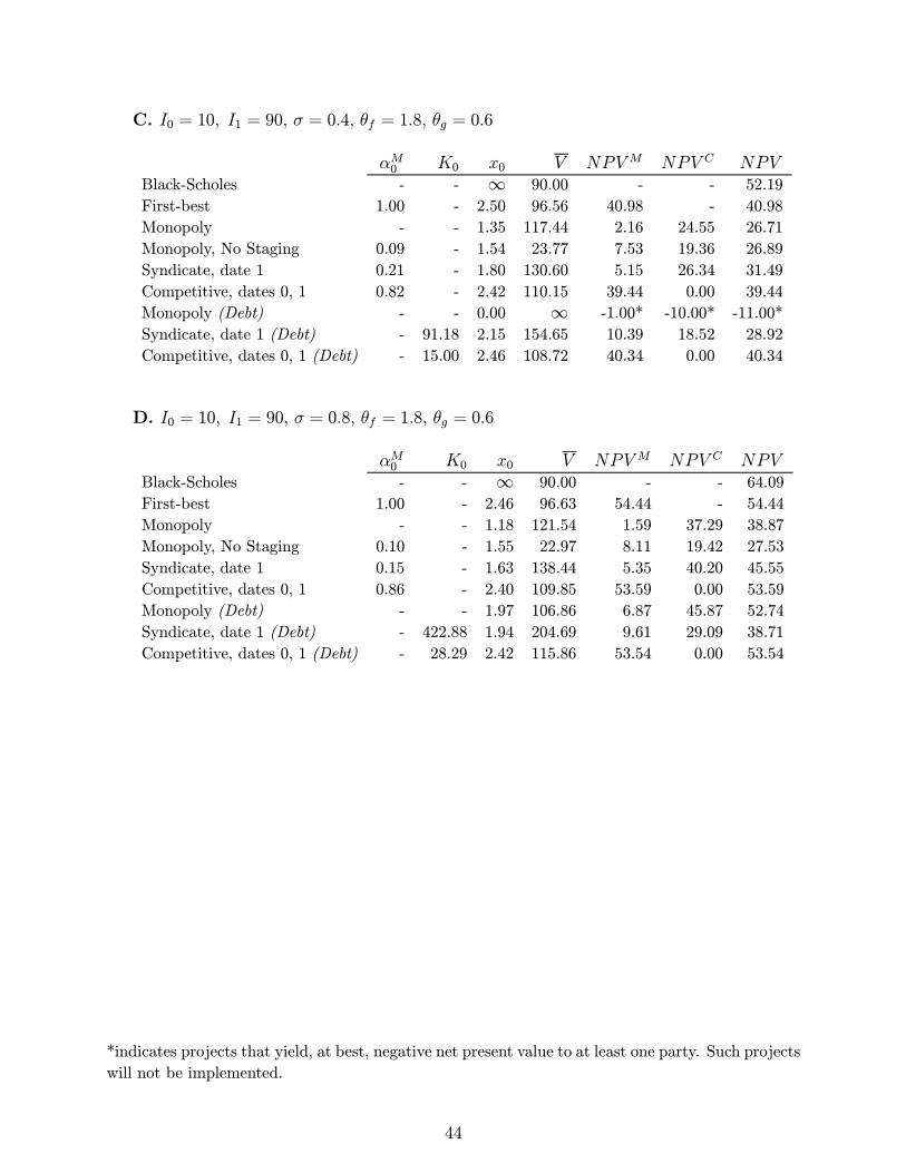
C. I0 = 10, I1 = 90, σ = 0.4, θf = 1.8, θg = 0.6

αM0 K0 x0 V NPV M NPV C NPVBlack-Scholes - - ∞ 90.00 - - 52.19

First-best 1.00 - 2.50 96.56 40.98 - 40.98

Monopoly - - 1.35 117.44 2.16 24.55 26.71

Monopoly, No Staging 0.09 - 1.54 23.77 7.53 19.36 26.89

Syndicate, date 1 0.21 - 1.80 130.60 5.15 26.34 31.49

Competitive, dates 0, 1 0.82 - 2.42 110.15 39.44 0.00 39.44

Monopoly (Debt) - - 0.00 ∞ -1.00* -10.00* -11.00*

Syndicate, date 1 (Debt) - 91.18 2.15 154.65 10.39 18.52 28.92

Competitive, dates 0, 1 (Debt) - 15.00 2.46 108.72 40.34 0.00 40.34

D. I0 = 10, I1 = 90, σ = 0.8, θf = 1.8, θg = 0.6

αM0 K0 x0 V NPV M NPV C NPVBlack-Scholes - - ∞ 90.00 - - 64.09

First-best 1.00 - 2.46 96.63 54.44 - 54.44

Monopoly - - 1.18 121.54 1.59 37.29 38.87

Monopoly, No Staging 0.10 - 1.55 22.97 8.11 19.42 27.53

Syndicate, date 1 0.15 - 1.63 138.44 5.35 40.20 45.55

Competitive, dates 0, 1 0.86 - 2.40 109.85 53.59 0.00 53.59

Monopoly (Debt) - - 1.97 106.86 6.87 45.87 52.74

Syndicate, date 1 (Debt) - 422.88 1.94 204.69 9.61 29.09 38.71

Competitive, dates 0, 1 (Debt) - 28.29 2.42 115.86 53.54 0.00 53.54

*indicates projects that yield, at best, negative net present value to at least one party. Such projects

will not be implemented.

44

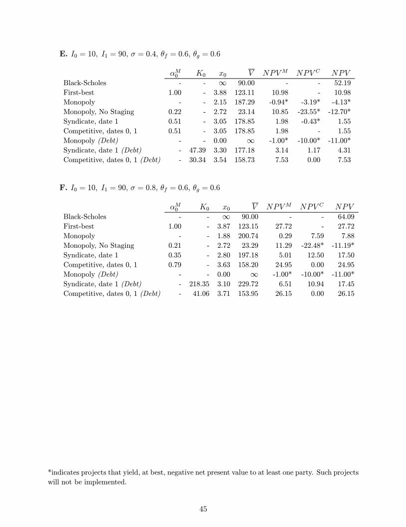
E. I0 = 10, I1 = 90, σ = 0.4, θf = 0.6, θg = 0.6

αM0 K0 x0 V NPV M NPV C NPVBlack-Scholes - - ∞ 90.00 - - 52.19

First-best 1.00 - 3.88 123.11 10.98 - 10.98

Monopoly - - 2.15 187.29 -0.94* -3.19* -4.13*

Monopoly, No Staging 0.22 - 2.72 23.14 10.85 -23.55* -12.70*

Syndicate, date 1 0.51 - 3.05 178.85 1.98 -0.43* 1.55

Competitive, dates 0, 1 0.51 - 3.05 178.85 1.98 - 1.55

Monopoly (Debt) - - 0.00 ∞ -1.00* -10.00* -11.00*

Syndicate, date 1 (Debt) - 47.39 3.30 177.18 3.14 1.17 4.31

Competitive, dates 0, 1 (Debt) - 30.34 3.54 158.73 7.53 0.00 7.53

F. I0 = 10, I1 = 90, σ = 0.8, θf = 0.6, θg = 0.6

αM0 K0 x0 V NPV M NPV C NPVBlack-Scholes - - ∞ 90.00 - - 64.09

First-best 1.00 - 3.87 123.15 27.72 - 27.72

Monopoly - - 1.88 200.74 0.29 7.59 7.88

Monopoly, No Staging 0.21 - 2.72 23.29 11.29 -22.48* -11.19*

Syndicate, date 1 0.35 - 2.80 197.18 5.01 12.50 17.50

Competitive, dates 0, 1 0.79 - 3.63 158.20 24.95 0.00 24.95

Monopoly (Debt) - - 0.00 ∞ -1.00* -10.00* -11.00*

Syndicate, date 1 (Debt) - 218.35 3.10 229.72 6.51 10.94 17.45

Competitive, dates 0, 1 (Debt) - 41.06 3.71 153.95 26.15 0.00 26.15

*indicates projects that yield, at best, negative net present value to at least one party. Such projects

will not be implemented.

45

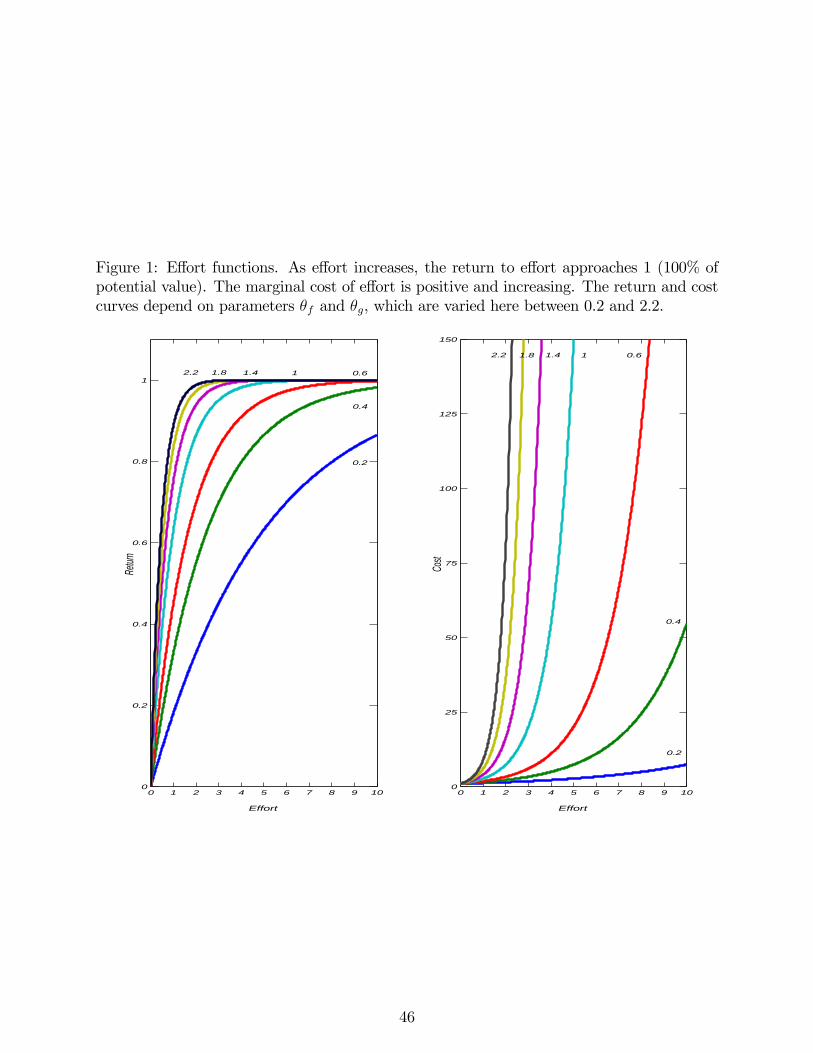
Figure 1: Effort functions. As effort increases, the return to effort approaches 1 (100% ofpotential value). The marginal cost of effort is positive and increasing. The return and costcurves depend on parameters θf and θg, which are varied here between 0.2 and 2.2.

0 1 2 3 4 5 6 7 8 9 100

0.2

0.4

0.6

0.8

1

Effort

Retur

n

0 1 2 3 4 5 6 7 8 9 100

25

50

75

100

125

150

Effort

Cost

0.2

0.4

0.6 1 1.4 1.8

1.4 1 0.6

0.2

0.4

2.2 1.8

2.2

46

Figure 2: Date-1 Net present values are plotted against V1, the date-1 realization of maximumpotential value. Potential value is V0 = E0(V2) = 150. The lognormal probability densityis plotted for a standard deviation of 0.4. Date-1 investment is I1 = 50. With no costs ofeffort, NPV1 = V1 − I1. When effort is costly, the level and slope of NPV1 decline becauseof reduced effort at date 0 (the optimal effort x0 is too low to attain maximum potentialvalue). The strike value V 1, which incorporates the cost of date-1 effort, increases from I1to I1 + g(x1) = 70.84.

0 50 100 150 200 250 300 350 400 4500

50

100

150

200

250

300

350

400NPV

1(x

0)

Prob(V1)

V1 V

0 V

1

V1 − I

1

NPV1(x

0* )

I0

I0 + g

0*

|

47

Figure 3: Net Present Value at date 0 in the first-best scenario. NPV is shown across arange of standard deviation (σ ∈ [0.1, 1.2]) and effort return (θf/θg ∈ [1/11, 11]) parameters.The dark surface presents date-0 and date-1 investment levels I0 = I1 = 50 while the lightsurface presents I0 = 10, I1 = 90. Potential value is V0 = E0(V2) = 150.

48

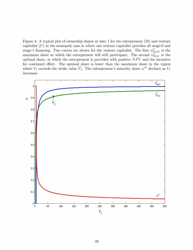
Figure 4: A typical plot of ownership shares at date 1 for the entrepreneur (M) and venturecapitalist (C) in the monopoly case in where one venture capitalist provides all stage-0 andstage-1 financing. Two curves are shown for the venture capitalist. The first αC

MAX is themaximum share at which the entrepreneur will still participate. The second αC

FOC is theoptimal share, at which the entrepreneur is provided with positive NPV and the incentivefor continued effort. The optimal share is lower than the maximum share in the regionwhere V1 exceeds the strike value V1. The entrepreneur’s minority share αM declines as V1increases.

0 50 100 150 200 250 300 350 400 450 5000

0.1

0.2

0.3

0.4

0.5

0.6

0.7

0.8

0.9

1

α

V1

αCFOC

αCMAX

αM

V1

49

Figure 5: Net Present Value at date 0, plotted for the Monopoly and Monopoly, No Stagingfinancing scenarios. NPV is shown across a range of standard deviation (σ ∈ [0.1, 1.2])and effort return (θf/θg ∈ [1/11, 11]) parameters. The dark surface presents non-stagedNPV s while the light surface presents staged NPV s. Figure 5 assumes date-0 and date-1investment levels I0 = I1 = 50 and potential value of V0 = E0(V2) = 150.

50

Figure 6: Net Present Value at date 0, plotted for the Monopoly and Monopoly, No Stagingfinancing scenarios. NPV is shown across a range of standard deviation (σ ∈ [0.1, 1.2])and effort return (θf/θg ∈ [1/11, 11]) parameters. The dark surface presents non-stagedNPV s while the light surface presents staged NPV s. Figure 6 assumes date-0 and date-1investment levels I0 = 10, I1 = 90 and potential value of V0 = E0(V2) = 150.

51

Figure 7: A typical plot of ownership shares at date 1 for the entrepreneur (M), initial venturecapitalist (C) and syndicate of new investors (S) for the syndicate case. The syndicateprovides financing on competitive terms (NPV = 0) whenever V1 exceeds the strike valueV1, which is higher than in the monopoly case shown in Figure 4. The syndicate’s optimalshare αS

FOC is lower than the maximum share αSMAX at which the entrepreneur would still

participate. The constrained share αS declines as V1 increases, while the ownership sharesheld by the entrepreneur and incumbent venture capitalist increase with V1.

0 50 100 150 200 250 300 350 400 450 5000

0.1

0.2

0.3

0.4

0.5

0.6

0.7

0.8

0.9

1

α αS

FOC

αSMAX

αM

V1

αS

αC

V1

52

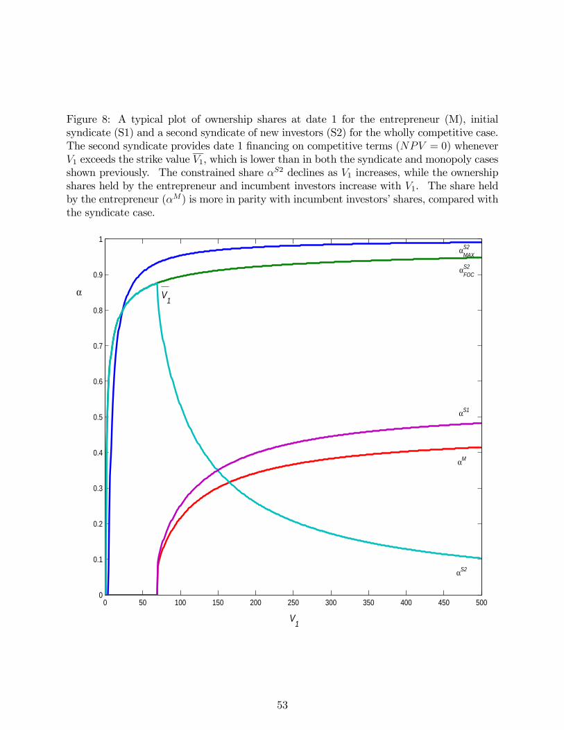
Figure 8: A typical plot of ownership shares at date 1 for the entrepreneur (M), initialsyndicate (S1) and a second syndicate of new investors (S2) for the wholly competitive case.The second syndicate provides date 1 financing on competitive terms (NPV = 0) wheneverV1 exceeds the strike value V1, which is lower than in both the syndicate and monopoly casesshown previously. The constrained share αS2 declines as V1 increases, while the ownershipshares held by the entrepreneur and incumbent investors increase with V1. The share heldby the entrepreneur (αM) is more in parity with incumbent investors’ shares, compared withthe syndicate case.

0 50 100 150 200 250 300 350 400 450 5000

0.1

0.2

0.3

0.4

0.5

0.6

0.7

0.8

0.9

1

V1

α

αS2MAX

αS2FOC

αS1

αM

αS2

V1

53

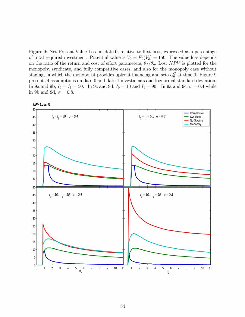
Figure 9: Net Present Value Loss at date 0, relative to first best, expressed as a percentageof total required investment. Potential value is V0 = E0(V2) = 150. The value loss dependson the ratio of the return and cost of effort parameters, θf/θg. Lost NPV is plotted for themonopoly, syndicate, and fully competitive cases, and also for the monopoly case withoutstaging, in which the monopolist provides upfront financing and sets αC

0 at time 0. Figure 9presents 4 assumptions on date-0 and date-1 investments and lognormal standard deviation.In 9a and 9b, I0 = I1 = 50. In 9c and 9d, I0 = 10 and I1 = 90. In 9a and 9c, σ = 0.4 whilein 9b and 9d, σ = 0.8.

0 0.2 0.4 0.6 0.8 10

0.2

0.4

0.6

0.8

1

5

10

15

20

25

30

35

40

45

50

0 0.2 0.4 0.6 0.8 10

0.2

0.4

0.6

0.8

1

0 0.2 0.4 0.6 0.8 10

0.2

0.4

0.6

0.8

1

0 1 2 3 4 5 6 7 8 9 10 110

5

10

15

20

25

30

35

40

45

50

0 0.2 0.4 0.6 0.8 10

0.2

0.4

0.6

0.8

1

1 2 3 4 5 6 7 8 9 10 11

Competitive SyndicateNo StagingMonopoly

NPV Loss %

θr θ

r

I0 = I

1 = 50; σ = 0.4

I0 = 10, I

1 = 90; σ = 0.4

I0 = I

1 = 50; σ = 0.8

I0 = 10, I

1 = 90; σ = 0.8

54

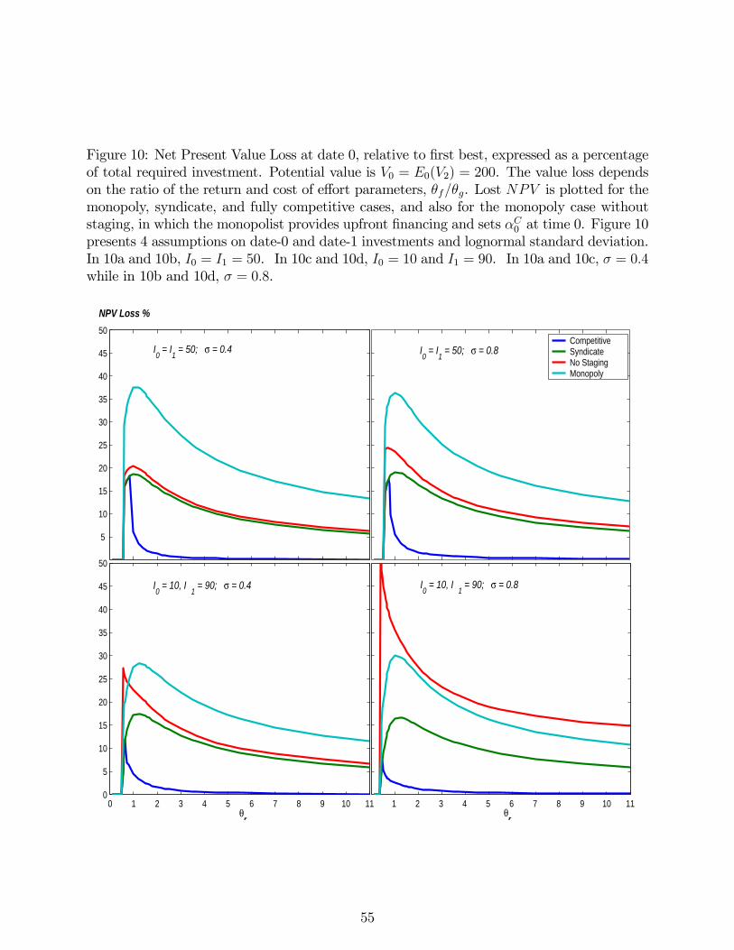
Figure 10: Net Present Value Loss at date 0, relative to first best, expressed as a percentageof total required investment. Potential value is V0 = E0(V2) = 200. The value loss dependson the ratio of the return and cost of effort parameters, θf/θg. Lost NPV is plotted for themonopoly, syndicate, and fully competitive cases, and also for the monopoly case withoutstaging, in which the monopolist provides upfront financing and sets αC

0 at time 0. Figure 10presents 4 assumptions on date-0 and date-1 investments and lognormal standard deviation.In 10a and 10b, I0 = I1 = 50. In 10c and 10d, I0 = 10 and I1 = 90. In 10a and 10c, σ = 0.4while in 10b and 10d, σ = 0.8.

0 5 10 150

10

20

30

40

0 5 10 150

10

20

30

40

0 5 10 150

5

10

15

20

25

30

0 5 10 150

10

20

30

40

50

60

5

10

15

20

25

30

35

40

45

50

0 1 2 3 4 5 6 7 8 9 10 110

5

10

15

20

25

30

35

40

45

50

1 2 3 4 5 6 7 8 9 10 11

Competitive SyndicateNo StagingMonopoly

θr θ

r

NPV Loss %

I0 = I

1 = 50; σ = 0.4 I

0 = I

1 = 50; σ = 0.8

I0 = 10, I

1 = 90; σ = 0.4 I

0 = 10, I

1 = 90; σ = 0.8

55