NBER WORKING PAPER SERIES

ALCOHOL ADVERTISING ANDALCOHOL CONSUMPTION BY ADOLESCENTS

Henry SafferDhaval Dave

Working Paper 9676http://www.nber.org/papers/w9676

NATIONAL BUREAU OF ECONOMIC RESEARCH1050 Massachusetts Avenue

Cambridge, MA 02138May 2003

The authors would like to thank Michael Grossman for his helpful comments. This project was funded byGrant Number R01 AA11851-02 from the National Institute on Alcohol Abuse and Alcoholism to theNational Bureau of Economic Research The views expressed herein are those of the authors and notnecessarily those of the National Bureau of Economic Research.

©2003 by Henry Saffer and Dhaval Dave. All rights reserved. Short sections of text not to exceed twoparagraphs, may be quoted without explicit permission provided that full credit including ©notice, is givento the source.

Alcohol Advertising and Alcohol Consumption by AdolescentsHenry Saffer and Dhaval DaveNBER Working Paper No. 9676May 2003JEL No. I1

ABSTRACT

The purpose of this paper is to empirically estimate the effects of alcohol advertising on adolescentalcohol consumption. The theory of brand capital is used to explain the effects of advertising onconsumption. The industry response function and the evidence from prior studies indicate that theempirical strategy should maximize the variance in the advertising data. The approach in this paperto maximizing the variance in advertising data is to employ cross sectional data. The Monitoringthe Future (MTF) and the National Longitudinal Survey of Youth 1997 (NLSY97) data sets, whichinclude only data for adolescents, are employed for the empirical work. These data sets areaugmented with alcohol advertising data, originating on the market level, for five media. Use ofboth the MTF and the NLSY97 data sets improves the empirical analysis since each data set has itsown unique advantages. The large size of the MTF makes it possible to estimate regressions withrace and gender specific subsamples. The panel nature of the NLSY97 makes it possible to estimateindividual fixed effects models. In addition, very similar models can be estimated with both datasets. Since the data sets are independent, the basically consistent findings increase the confidencein all the results. The results indicate that blacks participate in alcohol less than whites and theirparticipation cannot be explained with the included variables as well as it can for whites. Acomparison of male and female regressions shows that price and advertising effects are generallylarger for females. Models which control for individual heterogeneity result in larger advertisingeffects implying that the MTF results may understate the effect of alcohol advertising. The resultsbased on the NLSY97 suggest that a compete ban on all alcohol advertising could reduce adolescentmonthly alcohol participation by about 24 percent and binge participation by about 42 percent. Thepast month price-participation elasticity was estimated at about -0.28 and the price-bingeparticipation elasticity was estimated at about -0.51. Both advertising and price policies are shownto have the potential to substantially reduce adolescent alcohol consumption.

Henry Saffer Dhaval DaveNational Bureau of Economic Research National Bureau of Economic Research365 Fifth Avenue 5th floor 365 Fifth Avenue 5th floorNew York NY 10016-4309 New York NY 10016-4309hsaffer@gc.cuny.edu ddave@gc.cuny.edu

1. Introduction

Public health advocates have expressed concern that alcohol advertising is a factor

contributing to adolescent alcohol consumption. Both the level of alcohol consumption by

adolescents and the level of alcohol advertising are considerable. Data from the 2001 Monitoring

the Future Surveys (MTF) show that 7.7 percent of 8th graders, 21.9 percent of 10th graders and 49.8

percent of 12th graders consumed alcohol within the past 30 days (Johnston, O’Malley, Bachman,

2002). A Federal Trade Commission (FTC) report (1999) documents several outcomes associated

with underage drinking. These include reduced educational attainment, increased fatal motor

vehicle crashes, increased suicide attempts and increases in sexually transmitted diseases. The

probability of alcohol problems in adulthood also increases as the age of alcohol onset decreases.

Competitive Media Reporting (CMR) estimated that alcohol producers spent about $1.5 billion on

measured media advertising in 2001. This was a 25 percent increase over spending in 1998.

Alcohol industry reports to the FTC suggest that measured media advertising account for only one

half to one third of total promotional expenditures. Other forms of alcohol promotion include:

sponsorships; internet advertising; point-of-purchase advertising; consumer novelties; product

placements in movies and TV shows; direct mail; price promotions; and trade promotions directed

at wholesalers and retailers. These expenditures may enhance the effectiveness of measured media

spending.

Although there is a considerable level of alcohol advertising, the alcohol industry argues

that its advertising codes prohibit content and placement of advertising which target underage

individuals. The advertising codes require that more than 50 percent of the exposed audience be

over 21. The advertising codes also prohibit use of actors who appear underage and prohibit the use

2

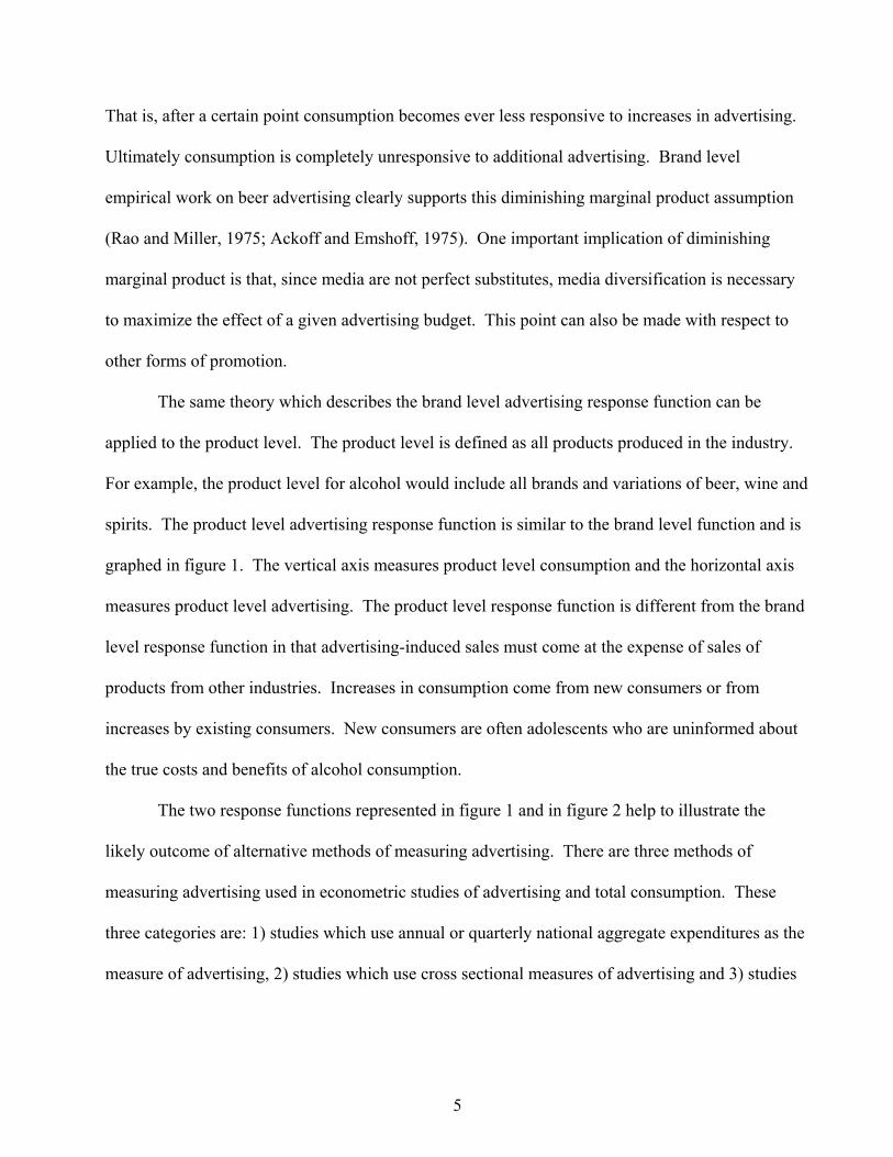
of Santa Claus. Cartoon characters, however, are not restricted and beer advertisers have no

restrictions on the use of sports celebrities.1

The Center on Alcohol Marketing and Youth (2002) examined the exposure of youth to

alcohol advertising in magazines, on TV and on radio. Youth are defined as individuals under the

age of 21. They found that in 2001, advertisers delivered 45 percent more beer advertising to youth

than to adults in magazines. For spirits, 27 percent more magazine advertising was delivered to

youth than to adults. However, for wine youths saw 58 percent less advertising than adults. Young

adults, defined as ages 21 to 34, were exposed to slightly more magazine alcohol advertising than

those under 21. Adults over 34 were exposed to the least amount of alcohol advertising in

magazines. They also found that on TV underage youth were exposed to two beer or ale ads for

every three seen by an adult. Beer and ale ads on TV represent about half of all alcohol advertising

in all media. On radio, youth heard 8 percent more beer and ale advertising, 12 percent more

malternative advertising and 14 percent more advertising for distilled spirits than adults 21 and

older. Youth heard substantially less radio advertising for wine. Grube (1995) reviews research on

the effect of alcohol advertising on knowledge, attitudes and intentions to drink by adolescents. He

finds that much of the imagery in alcohol advertising does appeal to youth and that this advertising

increases positive expectations about alcohol.

Studies of advertising exposure has led some public health groups to conclude that there is a

link between advertising and adolescent alcohol consumption. The Robert Wood Johnson

Foundation (1999) concludes that alcohol advertising and marketing are factors in the environment

that help create problems of underage drinking. There is, however, very little empirical evidence

that alcohol advertising has any effect on actual alcohol consumption (see for example, Nelson,

1 The beer, wine and spirits industries each have a somewhat different advertising code.

3

1999 or Fisher, 1993). Although both the level of alcohol consumption among adolescents and the

level of alcohol advertising are substantial and well documented, the link between the two remains

a controversial subject. There are no econometric studies of the effect of alcohol advertising on

adolescent drinking. The purpose of this paper is to provide these empirical estimates. The empirical

models include gender and race specific regressions of the effect of alcohol advertising.

2. Theoretical Framework

Competition through advertising, rather than price, is often preferred in industries that are

highly concentrated, such as the alcohol industry.2 Schmalensee (1972) shows that oligopoly firms

are likely to advertise more than similar firms in monopoly situations. Oligopoly firms attempt to

increase their share of the market with advertising rather than with price competition. Each firm

will be reluctant to use price competition if they believe that their rivals will also cut price. If all

firms cut price, they all move down an inelastic demand function similar to the industry demand

function. Share of market will not increase and revenue will decline. Advertising research usually

finds that the firm with the largest share of voice has the largest share of market.3 Each firm

attempts to advertise more than their rivals, which results in a high level of industry advertising.

The advertising-to-sales ratio for the alcohol industry is about nine percent, while the average for all

industries is about three percent (Advertising Age, 1999).

Becker and Murphy (1993) argue that advertising can be viewed as a complement to the

advertised good. They define the complementary good as a favorable image about the advertised

good. This increases the marginal utility of consumption and thus increases demand. Becker and

Murphy’s concept can be expanded somewhat and placed in the context of advertising theory.

Since advertising has a cumulative effect, the complementary good can be described as a stock and

2 This is less true for wine than for beer and spirits.

4

in advertising theory is called brand capital. Brand capital is defined as the collective positive

associations that individuals have about a brand. Advertising is one method of adding to or altering

brand capital. Brand capital depreciates over time and at differential rates for different brands. As

brand capital depreciates, a firm can attempt to offset the resulting decreases in sales with the

creation of additional brand capital. Depending on the relative marginal costs and marginal

benefits, the additions to brand capital can come in the form of new brands or from changes in the

content and level of advertising for existing brands. If advertising were banned, there would only

be limited possibilities to offset brand capital depreciation. This would reduce the marginal utility

of consumption and reduce sales.

Empirical studies of alcohol advertising estimate an alcohol demand equation. The alcohol

demand function is derived by assuming that a consumer maximizes a utility function, which

includes alcohol as one of its arguments, subject to a budget constraint. The complementarity of

brand capital suggests that alcohol advertising will increase the marginal utility of alcohol and thus

increase demand. This optimization problem results in an equation which shows that the demand

for alcohol is a function of alcohol price, alcohol advertising, and other variables affecting alcohol

demand such as income, availability of alcohol, alcohol sentiment and other taste variables.

Aggregating across consumers results in the market demand function.

Economic theory predicts that the relationship between advertising and consumption is

subject to diminishing marginal product. This concept is the basis of the advertising response

function. Advertising response functions have been used in brand level research to illustrate the

effect of advertising on consumption at various levels of advertising. Economic theory suggests

that due to diminishing marginal product, advertising response functions flatten out at some point.

3 Share of voice is the firm’s advertising as a percent of total industry advertising.

5

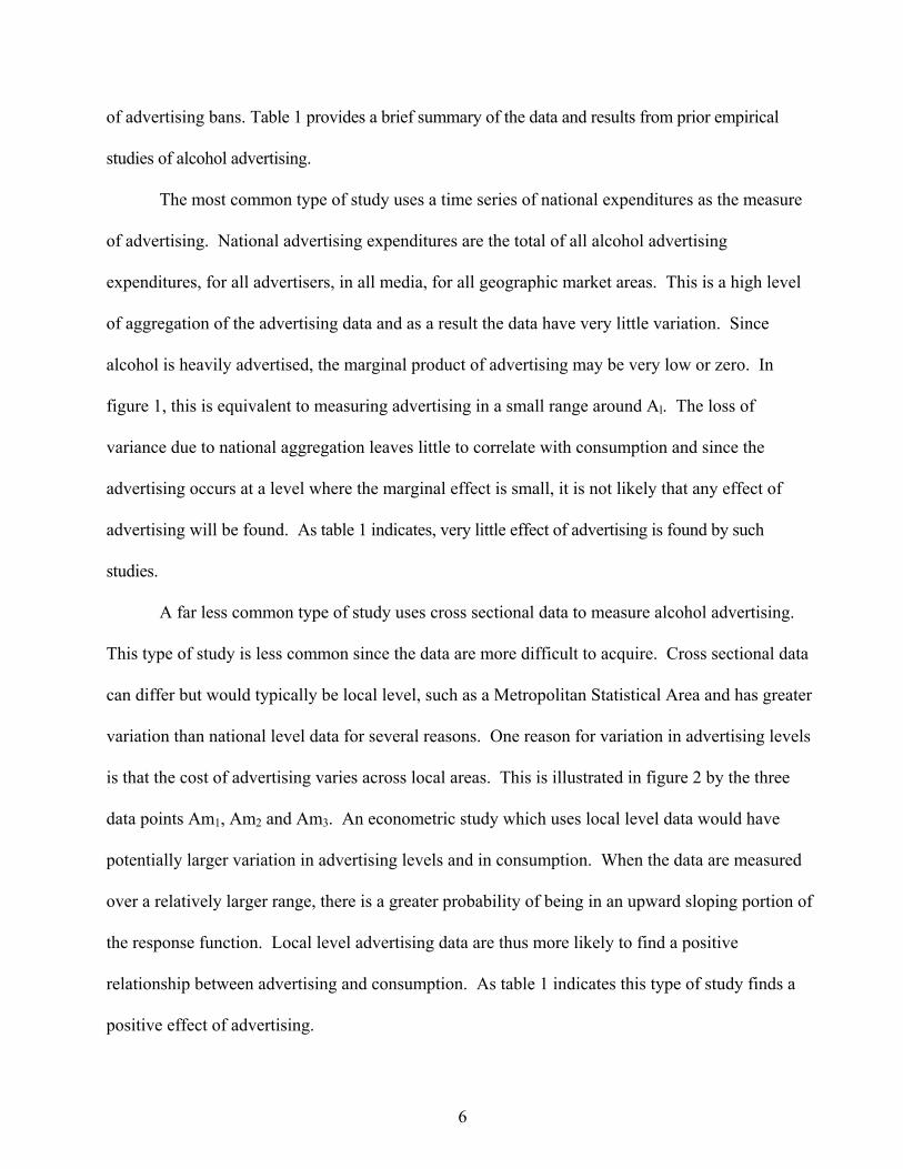
That is, after a certain point consumption becomes ever less responsive to increases in advertising.

Ultimately consumption is completely unresponsive to additional advertising. Brand level

empirical work on beer advertising clearly supports this diminishing marginal product assumption

(Rao and Miller, 1975; Ackoff and Emshoff, 1975). One important implication of diminishing

marginal product is that, since media are not perfect substitutes, media diversification is necessary

to maximize the effect of a given advertising budget. This point can also be made with respect to

other forms of promotion.

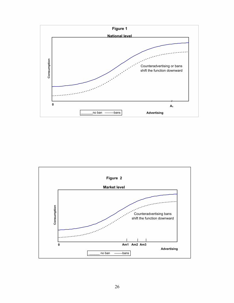
The same theory which describes the brand level advertising response function can be

applied to the product level. The product level is defined as all products produced in the industry.

For example, the product level for alcohol would include all brands and variations of beer, wine and

spirits. The product level advertising response function is similar to the brand level function and is

graphed in figure 1. The vertical axis measures product level consumption and the horizontal axis

measures product level advertising. The product level response function is different from the brand

level response function in that advertising-induced sales must come at the expense of sales of

products from other industries. Increases in consumption come from new consumers or from

increases by existing consumers. New consumers are often adolescents who are uninformed about

the true costs and benefits of alcohol consumption.

The two response functions represented in figure 1 and in figure 2 help to illustrate the

likely outcome of alternative methods of measuring advertising. There are three methods of

measuring advertising used in econometric studies of advertising and total consumption. These

three categories are: 1) studies which use annual or quarterly national aggregate expenditures as the

measure of advertising, 2) studies which use cross sectional measures of advertising and 3) studies

6

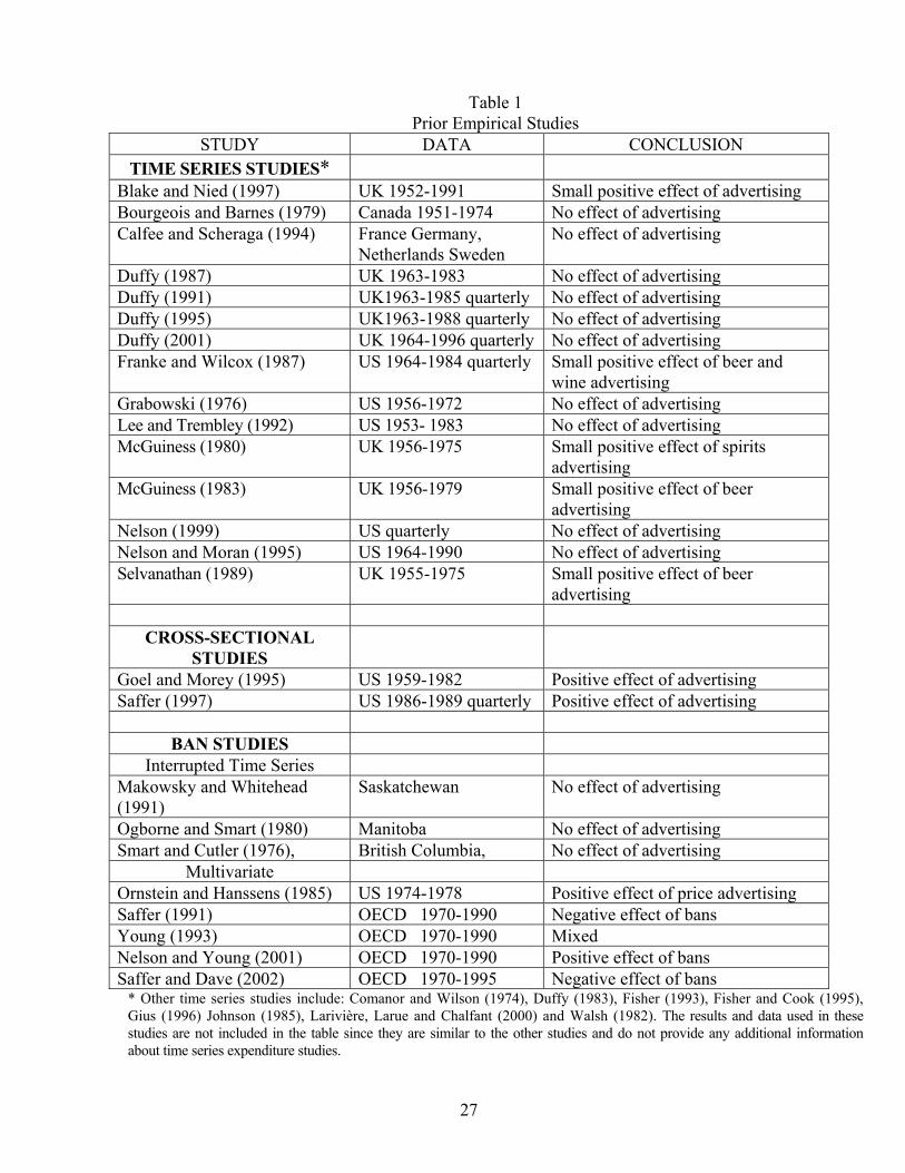
of advertising bans. Table 1 provides a brief summary of the data and results from prior empirical

studies of alcohol advertising.

The most common type of study uses a time series of national expenditures as the measure

of advertising. National advertising expenditures are the total of all alcohol advertising

expenditures, for all advertisers, in all media, for all geographic market areas. This is a high level

of aggregation of the advertising data and as a result the data have very little variation. Since

alcohol is heavily advertised, the marginal product of advertising may be very low or zero. In

figure 1, this is equivalent to measuring advertising in a small range around Al. The loss of

variance due to national aggregation leaves little to correlate with consumption and since the

advertising occurs at a level where the marginal effect is small, it is not likely that any effect of

advertising will be found. As table 1 indicates, very little effect of advertising is found by such

studies.

A far less common type of study uses cross sectional data to measure alcohol advertising.

This type of study is less common since the data are more difficult to acquire. Cross sectional data

can differ but would typically be local level, such as a Metropolitan Statistical Area and has greater

variation than national level data for several reasons. One reason for variation in advertising levels

is that the cost of advertising varies across local areas. This is illustrated in figure 2 by the three

data points Am1, Am2 and Am3. An econometric study which uses local level data would have

potentially larger variation in advertising levels and in consumption. When the data are measured

over a relatively larger range, there is a greater probability of being in an upward sloping portion of

the response function. Local level advertising data are thus more likely to find a positive

relationship between advertising and consumption. As table 1 indicates this type of study finds a

positive effect of advertising.

7

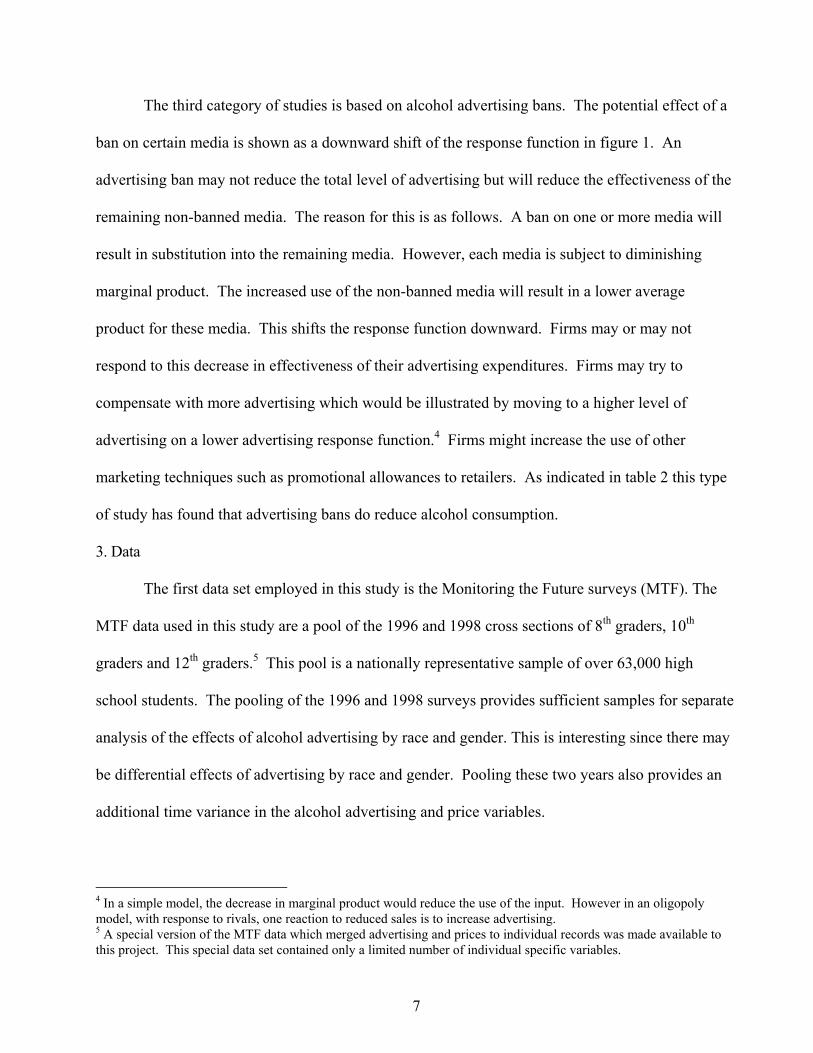
The third category of studies is based on alcohol advertising bans. The potential effect of a

ban on certain media is shown as a downward shift of the response function in figure 1. An

advertising ban may not reduce the total level of advertising but will reduce the effectiveness of the

remaining non-banned media. The reason for this is as follows. A ban on one or more media will

result in substitution into the remaining media. However, each media is subject to diminishing

marginal product. The increased use of the non-banned media will result in a lower average

product for these media. This shifts the response function downward. Firms may or may not

respond to this decrease in effectiveness of their advertising expenditures. Firms may try to

compensate with more advertising which would be illustrated by moving to a higher level of

advertising on a lower advertising response function.4 Firms might increase the use of other

marketing techniques such as promotional allowances to retailers. As indicated in table 2 this type

of study has found that advertising bans do reduce alcohol consumption.

3. Data

The first data set employed in this study is the Monitoring the Future surveys (MTF). The

MTF data used in this study are a pool of the 1996 and 1998 cross sections of 8th graders, 10th

graders and 12th graders.5 This pool is a nationally representative sample of over 63,000 high

school students. The pooling of the 1996 and 1998 surveys provides sufficient samples for separate

analysis of the effects of alcohol advertising by race and gender. This is interesting since there may

be differential effects of advertising by race and gender. Pooling these two years also provides an

additional time variance in the alcohol advertising and price variables.

4 In a simple model, the decrease in marginal product would reduce the use of the input. However in an oligopoly model, with response to rivals, one reaction to reduced sales is to increase advertising. 5 A special version of the MTF data which merged advertising and prices to individual records was made available to this project. This special data set contained only a limited number of individual specific variables.

8

The MTF surveys provide data on drinking occasions in the past year as well as the past

month and the number of times in the past two weeks that the respondent had five or more drinks in

one occasion. Three dichotomous alcohol participation variables were constructed from these data.

These are past year participation, past month participation and binge participation. The binge

drinking variable is defined as one if the youth had at least one drinking occasion in the two weeks

prior to the survey in which five or more drinks were consumed, and is zero otherwise. Binge

drinking represents those occasions most likely to have negative consequences and to be of concern

to policy makers (i.e., drinking five or more drinks in a single occasion and then driving is expected

to significantly raise the probability of a motor vehicle accident and, potentially, death).

Several independent variables were constructed from the socioeconomic and demographic

questions included in the surveys. These variables are: the individual’s income, gender, age and

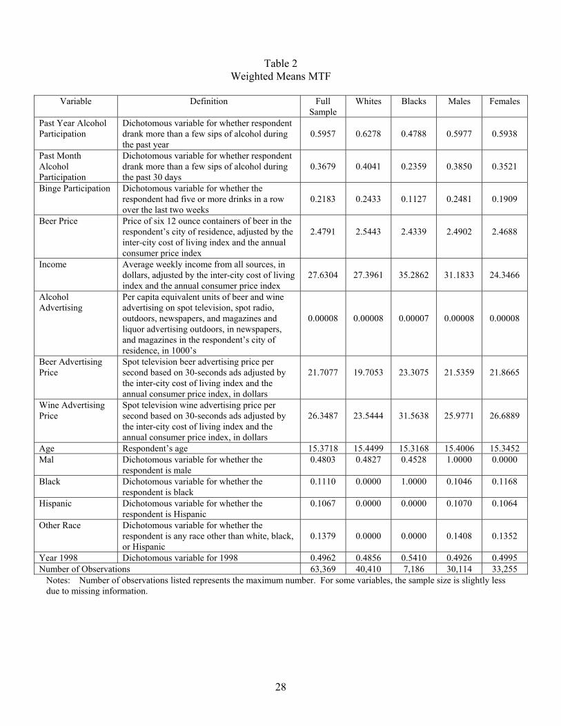
race (white, black, Hispanic or other)6. The regressions also include a single time dummy. Table 2

provides summary definitions and means for the variables which were used in the regressions with

the MTF data.

The second data set employed in this study is the National Longitudinal Survey of Youth

1997 (NLSY97). The sample consists of approximately 10,000 youths who live in the US and who

were 12 to 16 years old as of December 31, 1996. Using a statistically selected representative

sample of all households, based on the 1990 Census, the sample is representative of adolescents

nationwide. The NLSY97 data provide an important alternative to the MTF by including

individuals who are not in school and by including data collected from the parents. It is also a panel

data set, which allows for estimation of individual fixed effects models. The NLSY97 data set used

for the regressions was constructed from the 1997 and 1998 panels.

9

The NLSY97 surveys provide data on alcohol consumption and basic demographics. The

alcohol variables include past month alcohol participation and binge participation. Binge

participation is defined as one if the youth had at least one drinking occasion during the 30 days

prior to the survey in which five or more drinks were consumed, and is zero otherwise. The

independent variables constructed from the demographic questions include the individual's income,

gender, age and race (black, Hispanic or other).

In addition, the NLSY97 provides data on a number of other factors which may influence

alcohol consumption. The NLSY97 includes a set of questions on schooling, academic

achievement and aptitudes. These include a dichotomous variable equal to one for youths currently

not in school. A variable measuring years of schooling completed was also defined. Also, a

variable measuring the individual's math score on the Peabody Individual Achievement Test was

defined. In addition, a set of variables which measure parental supervision were defined. These

include a variable which measures how often the respondent eats dinner with their family. A

review by the Council of Economic Advisors (2000) found this variable to be a significant predictor

of alcohol use. Also, the respondents are asked to report the number of times during a typical week

that they do something religious as a family. The response data ranges from zero to seven.

Furthermore, a youth's ability to cope with stress and the difficulties of adolescence may affect their

alcohol consumption. Youths that report that they can get emotional support from their parents

may be less likely to use alcohol. An index of family relationship is provided in the NLSY97. This

index takes on values from zero to 32, with higher values indicating a closer relationship. In

addition, a household size variable is defined. Also a dichotomous variable equal to one if the

individual worked in the past year was defined. A dichotomous variable measuring the presence of

6The other category includes individuals who did not respond to the race question to minimize loss of data due to non-

10

another individual during the interview was also included. Finally, a year dummy is included.

Table 3 provides summary definitions and means for the variables which were used in the

regressions from the NLSY97.

Advertising data, alcohol price data and cost of living data are appended to both the MTF

and the NLSY97. Since 1996 and 1998 MTF data and 1997 and 1998 NLSY97 data are used in this

study, the advertising data which was purchased includes the years 1996 to 1998. The advertising

data come from Competitive Media Reporting (CMR). CMR collects advertising data in broadcast,

outdoor and other media. The reliability of these data is widely recognized in the advertising

industry. All of the data reported by CMR are independent estimates and do not use any

information from alcohol producers. The data are collected by monitoring the media, from

broadcast station reports and advertising wholesalers’ reports. Only alcohol advertising data with

local variation have been used in this study. Network television, syndicated television, cable

network television and network radio all have no local variation and in a regression model these

data would simply affect the intercept. Spot television, spot radio, outdoor and newspapers all have

local variation and are reported by advertising market areas. Magazine advertising can also be

included since national advertising expenditures and local circulation are available. Local

magazine advertising is estimated by multiplying national advertising by the percent of total

circulation in the local market. An advertising market area is known as a Designated Market Area

(DMA) and is similar to a Metropolitan Statistical Area. The advertising data were appended to the

individual records by DMA. This approach provides cross sectional variance in the advertising data,

which is an important empirical issue in measuring the effect of advertising. A single media

response. Excluding observations with missing race information does not materially change the results.

11

aggregated advertising variable is useful because it accounts for all media and media substitution

while avoiding problems of colinearity between media.

The advertising variable which is appended to the individual data should approximate the

exposure of an average youth to alcohol advertising. The local level alcohol advertising data that

are available include: spot television expenditures, spot radio expenditures, outdoor expenditures,

magazine expenditures and newspaper expenditures. National level advertising has no local

variation and is not included. The construction of the advertising variable assumes a competitive

market for advertising. Let:

Atv = a spot TV advertising message, Ai = an advertising message in other local media, i, Ptv = price of a TV advertising message, Pi = price of an advertising message in other local media, i and Ptv = qiPi where qi measures the impact of a TV advertisement relative to an advertisement in another local media. The advertising variable is constructed by converting all expenditure data to TV equivalent

messages. This conversion can be done by assuming that the price of a TV message relative to the

price of a message in another media is equal to impact of the TV message relative to the impact of a

message in another media. The price of TV advertising is calculated using data on number of seconds

and advertising expenditures on spot TV. The price per second is calculated from these data by

dividing expenditures by number of seconds which was done, by year, for each DMA. TV equivalent

messages for media i are Ai/qi. If A measures total TV equivalent messages, then A = Atv + Σ Ai/qi.

Since Atv can be multiplied by Ptv/Ptv, and 1/qi replaced by Pi/Ptv, then A = AtvPtv/Ptv + Σ AiPi/Ptv. Total

TV equivalent messages are thus equal to the sum of advertising expenditures on the five local media,

12

divided by the price of one second of spot TV advertising. Since the number of messages in a DMA

increases with population size, the total message variable is divided by DMA population.7

An important aspect of advertising is that its effects linger over time. That is, advertising in

one period will have a lingering, although an ever smaller effect, in subsequent periods. This could

be modeled as a Koyck transformation with constant rate of decay. A stock of advertising is created

since in each period new advertising is added to the depreciated advertising from prior periods.

However, the rate of decay from one period to the next is unknown and remains an arguable issue.

Research such as Boyd and Seldon (1990) finds that specific advertisements fully depreciate within

a year. An advertisement for a specific product helps create a personality for that product but it also

creates an expectancy about alcohol in general. Even if a specific advertisement completely decays

in less than a year, the expectancy about alcohol may linger for a longer period. If the decay rate

and structure were known, then a measure of stock could be calculated.

The dependent variables which are used in this paper are annual participation, monthly

participation and binge participation. Annual advertising can be matched to annual participation,

and annual advertising can be assumed to be a proxy for the stock of advertising when monthly

participation data are used.8 The regression results are interpreted as an estimate of the marginal

effect of an increase in annual advertising on annual, monthly alcohol participation and binge

participation.

Since beer is the most widely used alcoholic beverage by underaged drinkers the price of

beer is used in the demand functions. Data on the money price of beer was taken from the Inter-City

7 According to the Center on Alcohol Marketing and Youth, youth exposure is in the same range as overall population exposure. 8 The stock of advertising is equal to the current period advertising plus the discounted value of advertising from prior periods. Let advertising in each period be equal to an average value plus a positive or negative deviation from this average value. The sum of the discounted values of the deviations can be assumed to equal zero. The stock of

13

Cost of Living Index, published quarterly by the American Chamber of Commerce Researchers

Association (ACCRA). This data set includes prices for all the years and DMAs included in the

data sets. The ACCRA data contain the price of standard brands of beer for the years included in the

alcohol data sets.

The price of beer and income are adjusted for local cost of living and price changes over time.

Data on the local cost of living were taken from the Inter-City Cost of Living Index, published

quarterly by the American Chamber of Commerce Researchers Association (ACCRA). The

ACCRA cost of living index is based on over sixty categories of consumer purchases and uses

expenditure weights based on government survey data of expenditures of mid-management households.

The ACCRA cost of living index has no time variation and is indexed to one for the average cost of

living. Price changes over time were measured with the national CPI for all urban consumers reported

in Business Conditions Digest (Bureau of Economic Analysis, USDC). The cost of living index used to

adjust beer prices and income was computed by multiplying the ACCRA index by the national CPI.

4. Results

The first empirical issue is potential endogeneity between alcohol advertising and youth alcohol

participation. One source of endogeneity reflects the direction of causality. Current period advertising

could be a function of aggregate sales in the prior period for the overall population. However, in the

models estimated in this study, the dependent variables are dichotomous indicators of youth alcohol

participation, which may only be weakly correlated with consumption in the overall population.

Furthermore, while reverse causality may run from past period sales to current period advertising, the

models in this study estimate current period consumption as a function of current or past period

advertising. Thus, a priori, this source of endogeneity does not appear likely. Another form of

advertising will equal the average value times a factor which will be greater than one. The annual advertising is equal

14

endogeneity may be due to unobserved factors, which are correlated with both youth alcohol

participation and advertising. The extensive set of variables available in the NLSY97 and the

individual fixed effects models should account for this unobserved heterogeneity.

Nevertheless, the potential for endogeneity does remain. The alcohol participation equations

were tested with the Smith-Blundell and Wu-Hausman tests.9 This requires the specification of a

reduced form advertising demand function. This advertising demand function includes all of the

exogenous variables from the alcohol demand function and also the price of beer advertising on TV

and the price of wine advertising on TV.10 Advertising price strongly affects the level of

advertising, but has no direct effect on youth alcohol participation. Endogeneity was tested for

annual, monthly and binge participation for the MTF full sample, and for monthly and binge

participation for all specifications with the NLSY97 data. As expected, all nine tests rejected

endogeneity and the alcohol participation models are estimated with single equation techniques.

Table 4 presents the results from the estimation of 15 alternative specifications of the alcohol

demand equation with the MTF data. The table has three sections which follow the same pattern. Each

section contains five probit regressions which use alternative sample populations. The first regression

uses the full sample, the second and third limit the sample to whites and blacks, respectively, while the

fourth and fifth limit the sample to males and females, respectively. Each section presents results for a

different dependent variable.

The results for annual and monthly alcohol participation are presented in the first and second

section of table 4. For annual participation, alcohol advertising is positive and significant in four out of

to the average value times the number of periods. Annual advertising is thus proportional to the stock of advertising. 9 The Smith-Blundell test is a version of the Wu-Hausman test for exogeneity, applied to structural equations estimated as probit. This test, which is related to an auxiliary regression test for exogeneity, involves testing for the exclusion of the residual vector obtained from the first-stage regression. Under the null hypothesis, these residuals should have no explanatory power in the structural equation. See Smith and Blundell (1986). 10 Spirits did not use TV advertising during this period.

15

five regressions. For monthly participation, alcohol advertising is positive and significant in three

regressions. Two of these insignificant coefficients are for blacks and one is for males. Alcohol price is

negative and significant in all five annual participation regressions and negative and significant in three

monthly regressions. The two insignificant coefficients are again in the black and male regressions.

Income and age are positive and significant in all five regressions for both annual and monthly

participation. The Hispanic variable is never significant in the annual participation regressions and

negative and significant in two out of three monthly participation regressions. The other race variable

is negative and significant in all regressions.

The results for binge participation in the past two weeks are presented in section 3 of table 4 and

are similar to the other two alcohol use measures. Alcohol advertising is positive and significant in four

out of five regressions while alcohol price is negative and significant in three regressions. Income is

positive and significant in all five regressions and age is positive and significant in four regressions. The

Hispanic variable is negative and significant only in the female regression. The other race variable is

negative and significant in all three regressions indicating lower binge drinking.

The race specific regressions in table 4 allow for all the coefficients to vary between groups. A

comparison of white and black regressions shows that the coefficients are generally lower for blacks.

Also, the pseudo R-squares for blacks are about 0.03 while they are about 0.06 to 0.07 for whites. This

indicates that the regression equation can explain more of the variance in participation for whites than

for blacks. From the table of means, participation for whites is one and a half to two times higher than

participation for blacks. These differences in simple means are mirrored by the negative and significant

black variable in the regressions estimated with the full sample and the gender specific samples. The

marginal effects suggest that being black reduces the probability of past year and monthly alcohol

participation by about 18 percentage points. For binge participation, the marginal effect is about 14

16

percentage points, similar to the difference of 0.13 suggested by the simple means. Overall, the results

indicate that blacks participate less than whites and that their participation is less responsive to policy

than the participation by whites.

A comparison of male and female regressions in table 4 shows that for annual participation

price and advertising effects are larger for females but otherwise the coefficients are about the same.

For monthly participation and binge participation, price and advertising effects are significant for

females but not for males. However, the R-squares for males are larger than those for females. The

table of means shows that annual and monthly participation for males and females are about equal.

However, the male variable in the regressions estimated with the full sample and the race specific

samples is negative and significant for annual participation, and significantly positive for monthly and

binge participation. While the difference is not large, this indicates that when other factors are held

constant, male annual participation is somewhat less than that for females. When other factors are held

constant, males tend to have higher monthly participation than females. However, the male variable in

the white regression is not significant. Binge participation for males is also somewhat higher than for

females. This is also reflected in the male variable in the regressions estimated with the full sample and

the race specific samples which is positive and significant. Overall, the results indicate that males

participate more than females and that male participation is explained more by demographics than

public policy.

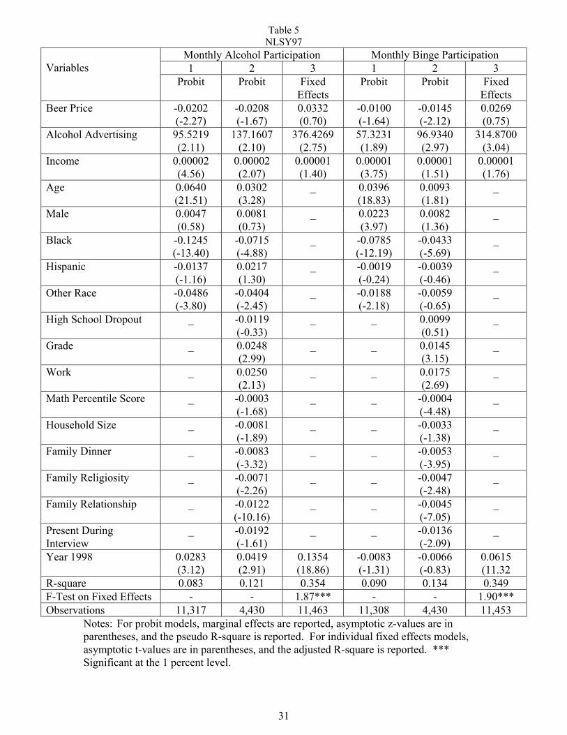
Table 5 presents the results from the estimation of six alcohol demand equations with the

NLSY97 data. Specifications 1 and 2 are estimated with probit. Specification 1 uses a limited set of

independent variables and is comparable to the MTF specification. Specification 2 uses an extended set

of independent variables, which are included to control for individual heterogeneity not controlled in

the limited specifications. Specification 3 limits the independent variables but includes a full set of

17

individual dummies and one time dummy variable. These dummy variable specifications control for all

individual specific time invariant unobservable factors and also controls for individual invariant time

specific factors. In these specifications, an included independent variable can only explain changes in

alcohol participation that occur for individuals across time. For this reason the included independent

variables are limited to advertising, price and income.

In table 5, alcohol advertising is positive and significant in all six regressions. The addition of

variables which control for a greater degree of individual heterogeneity results in larger advertising

coefficients. Alcohol price is negative and significant in four regressions and not significant in the two

fixed effects models. A regression of alcohol price on the individual and time dummies produced an R-

square of 0.98, which indicates that there is very little variation in alcohol prices across individuals over

time. For this reason the alcohol price variable has very little independent variance which might

correlate with participation and is insignificant. Income is positive and significant in four of the six

regressions. The F-tests on the individual dummy variables in both the fixed effects models are

significant indicating that these dummies have an effect on participation. The significance of the

dummies indicates that controlling for unobserved heterogeneity across individuals is important.

Specifications 1 and 2 include additional independent variables. Income, age, Hispanic and

other race are also included in the MTF. The results for these variables from both the MTF and

NLSY97 are very similar. Income is positive and significant in four out of six regressions. Age is

positive and significant in all four regressions. The Hispanic variable is insignificant but the other race

variable is negative and significant in three out of four regressions. Specification 2 includes a number

of added variables which may influence alcohol consumption. These include a dichotomous

variable equal to one for youths currently not in school which is insignificant in both regressions.

The work variable is positive and significant in both regressions. The years of schooling variable is

18

also positive and significant in both regressions. The measure of math achievement is negative and

significant in both regressions. The family variables (family dinner, family religiosity, family

relationship) are all negative and significant in both regressions. And finally, the variable

measuring the presence of another individual during the survey interview is negative and significant

in both regressions. This variable may account for youths who may have understated their true

alcohol use due to the presence of a parent or guardian during the interview.

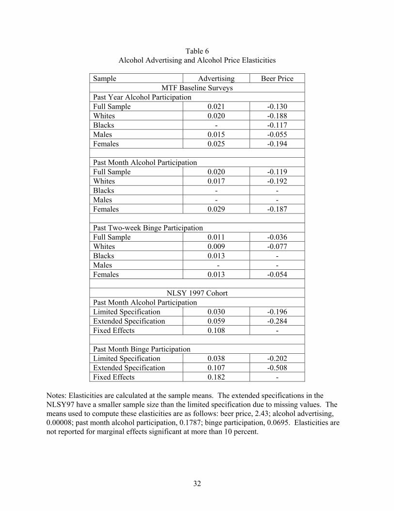
Table 6 presents the participation-advertising elasticities. From the MTF, the full sample

annual participation advertising elasticity is about 0.02. The past month participation-advertising

elasticity is about the same magnitude while the elasticity for binge participation is about half this size.

The elasticity estimates with the subsamples, where significant, follow this pattern. This regularity in

the results can be used to make a best guess for the insignificant black and male elasticities. The pattern

shows small differences by gender and race that have no substantive importance. From the NLSY97,

past month elasticity is about 0.03 in the limited specification. The elasticities estimated with the

extended specification and the fixed effects specifications are between 0.06 and 0.11. The binge

elasticity is about 0.04 in the limited specification and between 0.11 and 0.18 in the extended and fixed

effects specifications.

The elasticities presented in table 6 show the direction of bias due to heterogeneity. Table 6

presents alternative estimates of the advertising-past month participation elasticity from the MTF and

from the NLSY97. The estimated elasticities are very close in absolute terms. The same pattern is

evident in the binge drinking elasticities. The NLSY97 extended specification controls for more

heterogeneity than the limited specification and the fixed effects regressions control for all time

invariant individual heterogeneity. Table 6 shows that the elasticities increase as more controls for

heterogeneity are added. This suggests that heterogeneity bias results in an understatement of the effect

19

of advertising. The best guess elasticities are calculated from the NLSY97 extended and fixed effects

specifications. Averaging the NLSY97 elasticities for past month participation from the extended and

fixed effects models results in a value of about 0.08, and for binge participation results in a value of

about 0.14.

Table 6 also presents the participation price elasticities. From the MTF, the full sample past

year participation price elasticity is about -0.13. For past month, the magnitude is about the same and

for binge participation it is about one-third this size. The pattern shows small differences by race and

gender with lower values for blacks and higher values for females. From the NLSY97, past month

price elasticity is about -0.19 in the limited specification. The elasticity estimated with the extended

specification is higher at about -0.28. The binge elasticity is about -0.20 in the limited specification and

about -0.51 in the extended specification. This again suggests that controlling for individual

heterogeneity increases the elasticities and that the estimates from the MTF may understate the true

effect. The NLSY97 price elasticities for the extended specification may be the best since

heterogeneity is controlled to the best degree possible. These values are –0.28 for past month alcohol-

price participation, and –0.51 for binge-price participation.

5. Conclusions

Both the MTF and NLSY97 results contribute to the analyses and provide an important

comparison. The large size of the MTF data set makes it possible to estimate regressions with race

and gender specific subsamples. The panel nature of the NLSY97 makes it possible to estimate

individual fixed effects models. In addition very similar models can be estimated with both data

sets. Since the data sets are independent, the basically similar findings increase the confidence in

all the results.

20

The results from the MTF and the NLSY97 generally show that alcohol advertising has a

positive effect on annual alcohol participation, monthly participation and binge participation. Alcohol

price generally has a negative effect on these participation measures. Overall, the results indicate that

blacks participate less than whites and their participation cannot be explained with the included

variables as well as it can for whites. A comparison of male and female regressions shows that price

and advertising effects are generally larger for females, but otherwise the coefficients are about the

same. An important finding with the NLSY97 is that controlling for individual heterogeneity increases

the effects of advertising. This suggests that the results from the MTF may understate the true effects.

However, the relative black-white differences and male-female differences from the MTF are most

likely unaffected by the lack of control for heterogeneity.

The elasticity of advertising with respect to past month participation was estimated at about

0.08 and with respect to binge participation at about 0.14. Since only local advertising is included, the

actual range of potential reduction is around 300 percent. Local advertising is only about one-third of

total advertising expenditures. Thus the complete elimination of alcohol advertising would amount to a

300 percent reduction. This suggests that the compete elimination of alcohol advertising could reduce

adolescent monthly alcohol participation by about 24 percent and binge participation by about 42

percent.

The size of the price increases needed to result in a commensurate reduction can be

estimated with price elasticities. This provides a comparison of the effectiveness of advertising

reductions with tax increases as alternative policies. The price elasticities for past month

participation was estimated at about -0.28 and the binge participation elasticity at about -0.51. This

suggests that a 100 percent increase in alcohol prices would be needed to reduce adolescent monthly

alcohol participation by 28 percent, and this would reduce binge participation by 51 percent. For

21

monthly participation, the effect of a complete elimination of alcohol advertising would be similar to a

100 percent increase in alcohol prices. For binge participation, the effect of a complete elimination of

advertising would be equivalent to about an 80 percent increase in price. As a result, both advertising

and price policies are shown to have the potential to substantially reduce adolescent alcohol

participation.

22

References Ackoff, R. and J. Emshoff, “Advertising Research at Anheuser-Busch, Inc. (1963-68),” Sloan Management Review, Winter, p. 1-15, 1975. Advertising Age, Sales per Ad Dollar by Most Advertised Segment, www.adage.com, 1999. American Chamber of Commerce Researchers Association, ACCRA Cost of Living Index, Alexandria, Virginia, 1997-1999. Becker, G. and Murphy, K., “A Simple Theory of Advertising as a Good or Bad”, Quarterly Journal of Economics, 108, no. 4, 1993. Blake, D. and A. Nied, “The Demand for Alcohol in the United Kingdom”, Applied Economics, 29, 1655-1672, 1997. Bourgeois, J. and J. Barnes, "Does Advertising Increase Alcohol Consumption?", Journal of Advertising Research 19, 1979, 19-29. Boyd, R. and B. Seldon, “The Fleeting Effect of Advertising”, Economic Letters, 34, 1990. Breed, W., Wallack, L., and Grube, J. "Alcohol Advertising in College Newspapers: A 7-Year Follow-up", College Health, vol. 38, May, 1990. Bureau of Economic Analysis, Business Conditions Digest, United States Department of Commerce, 1996-1999. Calfee, J. and C. Scheraga, “The Influence of Advertising on Alcohol Consumption: A Literature Review and An Econometric Analysis of Four European Nations,” International Journal of Advertising, vol. 13, no. 4, 1994. p. 287-310. Center for Media Education, Alcohol Advertising Targeted at Youth on the Internet: An Update, http://tap.epn.org, 1998. Center on Alcohol Marketing and Youth. Overexposed, Georgetown University, September 24, 2002. Center on Alcohol Marketing and Youth. Drops in the bucket, Georgetown University, February 3, 2003. Center on Alcohol Marketing and Youth. Radio Daze, Georgetown University, April 3, 2003. Comanor, W., and Wilson, T., Advertising and Market Power, Cambridge: Harvard University Press, 1974. Competitive Media Reporting, LNA/Media Watch Multi-Media Service, CMR, New York, 2001.

23

Council of Economic Advisors, Teens and Their Parents in the 21st Century, http://clinton4.nara.gov/media/pdf/CEAreport.pdf , 2000. Duffy, M., "The Demand for Alcoholic Drink in the United Kingdom, 1963-78", Applied Economics, 15, 1983, 125-140. Duffy, M., "Advertising and the Inter-product Distribution of Demand", European Economic Review, 31, 1987, 1051-1070. Duffy, M. "Advertising in Demand Systems: Testing a Galbraithian Hypothesis", Applied Economics, 23, 1991, 485-496. Duffy, M., “Advertising in Demand Systems for Alcoholic Drinks and Tobacco: A Comparative Study,” Journal of Policy Modeling, vol. 17 no. 6, p. 557-577, 1995. Duffy, M. “Advertising in Consumer Allocation Models: Choice if Functional Form”, Applied Economics, 33, 437-456, 2001. Federal Trade Commission, Self-regulation in the Alcohol Industry, A Review of Industry Efforts to Avoid Promoting Alcohol to Underage Consumers, www.ftc.gov, 1999. Fisher, J. Advertising, Alcohol Consumption, and Abuse, A Worldwide Survey, Greenwood Press: Westport, 1993. Fisher, J. and Cook, P., Advertising, Alcohol Consumption and Mortality: An Empirical Investigation, Westport CT, Greenwood Press, 1995 Franke, G. and G. Wilcox, "Alcoholic Beverage Advertising and Consumption in the United States, 1964-1984", Journal of Advertising, 16, 1987, 22-30. Gius, M. P., “Using panel data to determine the effect of advertising on brand-level distilled spirits sales” Journal of Studies on Alcohol, 57, 73-76, 1996. Goel, R., and M. Morey, “The Interdependence of Cigarette and Liquor Demand,” Southern Economic Journal, vol. 62, no. 2, p. 441-459, 1995. Grabowski, H. "The Effects of Advertising on the Interindustry Distribution of Demand", Explorations in Economic Research, 3, 21-75 1976. Grube, J. “Alcohol Portrayals and Alcohol Advertising on Television: Content and Effects on Children and Adolescents,” Alcohol Health and Research World, vol. 17, no. 1, p. 61-66, 1993. Grube, J. and L. Wallack, "Television beer Advertising and Drinking Knowledge, Beliefs, and Intentions among Schoolchildren", American Journal of Public Health, vol. 84, no. 2, Feb. 1994.

24

Grube, J. “Television Alcohol Portrayals, Alcohol Advertising, and Alcohol Expectancies Among Children and Adolescents”, Effects of the Mass Media on the Use and Abuse of Alcohol, Martin, S.E., and Mail, P., eds. Bethesda, MD: National Institute on Alcohol Abuse and Alcoholism, 1995, 105 – 121. Johnson, L., "Alternative Econometric Estimates of the Effects of Advertising on the Demand for Alcoholic Beverages in the United Kingdom", International Journal of Advertising, 4, 1985, 19-25. Johnston, L. P. O'Malley, and J. Bachman, National Survey Results on Drug Use From Monitoring the Future Study, 1975-1994: Volume 1, Secondary School Students, Rockville MD. NIDA, 2002. Kelly, K. and Edwards, R., “Image Advertisements for Alcohol Products: Is their Appeal Associated with Adolescent Intention to Drink?”, Adolescence, 33, 47-59, 1998. Larivière, E., Larue, B. and Chalfant, J., “Modeling the Demand for Alcoholic Beverages and Advertising Specifications”, Agricultural Economics, 22, 147-162, 2000. Lee, B. and V. Tremblay, "Advertising and the US Market Demand for Beer", Applied Economics, 24, 1992, 69-76. Maddala G. Limited Dependent and Qualitative Variables in Economics, Cambridge, England: Cambridge University Press, 1983. Makowsky, C., and P. Whitehead, “Advertising and Alcohol Sales: A Legal Impact Study,” Journal of Studies on Alcohol, vol. 52, no. 6, 1991. p. 555-566. Martin, S. et al. “Alcohol Advertising and Youth”, Alcohol Clinical and Experimental Research, 26(6), 900-906, 2002. McGuiness, T. "An Econometric Analysis of Total Demand for Alcoholic Beverages in the U.K. 1956-1975", Journal of Industrial Economics, 29, 85-105, 1980. McGuiness, T. "The Demand for Beer, Spirits and Wine in the UK, 1956-1979", in Grant, Plant and Williams, eds. Economics and Alcohol Gardner Press, Inc. New York. 1983, 238-242. Nelson J. Broadcast Advertising and US Demand for Alcoholic Beverages", Southern Economic Journal 65(4) 774-790, 1999. Nelson J. P. and Young, D. J. (2001). “Do advertising bans work? An international comparison”, International Journal of Advertising, 20, 273-296. Nelson J. and J. Moran, “Advertising and US Alcoholic Beverage Demand: System-Wide Estimates,” Applied Economics, vol. 27, 1995. p. 1225-1236. Ogborne, A., and Smart, R., Will Restrictions on Alcohol Advertising Reduce Alcohol Consumption?,” British Journal of Addiction, 75, 293-296 1980.

25

Ornstein, S. and Hanssens, D., "Alcohol Control Laws and the Consumption of Distilled Spirits and Beer", Journal of Consumer Research, 12, 200-213, 1985. Parker, B. "Exploring Life Themes and Myths in Alcohol Advertisements through a Meaning-Based Model of Advertising Experiences, Journal of Advertising, vol. xxvii no. 1, Spring, 1998. Rao, R. and P. Miller, “Advertising/Sales Response Functions”, Journal of Advertising Research, 15:7-15, 1975. Robert Wood Johnson Foundation, Advances, no.1, 1999. Saffer, H., "Alcohol Advertising Bans and Alcohol Abuse: An International Perspective,” Journal of Health Economics, 10., 65-79, 1991. Saffer, H., "Alcohol Advertising and Highway Fatalities,” Review of Economics and Statistics, 79, 431-442, 1997. Saffer, H., and Dave, D., “Alcohol Consumption and Alcohol Advertising Bans”, Applied Economics, 34, 2002, 1325-1334. Schmalensee, R. The Economics of Advertising, Amsterdam: North-Holland, 1972. Selvanathan, E., "Advertising and Alcohol Demand in the UK: Further Results", International Journal of Advertising, 8, 1989, 181-188. Smart, R. and Cutler R., "The Alcohol Advertising Ban in British Columbia: Problems and Effects on Beverage Consumption,” British Journal of Addiction, 71, 13-21 1976. Smith, R. J., and Blundell, R. W. “An Exogeneity Test for a Simultaneous Equation Tobit Model with an Application to Labor Supply.” Econometrica, vol. 54, no. 3, 1986, 679-685. Walsh B., "The Demand for Alcohol in the UK: A Comment", The Journal of Industrial Economics, vol. 30, no. 4, June 1982. Young, D., "Alcohol Advertising Bans and Alcohol Abuse: Comment", Journal of Health Economics, 12, 213-228, 1993.

26

National level

Counteradvertising or bansshift the function downward

0 A1

Advertising_______no ban ---------bans

Figure 1

Market level

Counteradvertising bansshift the function downward

0 Am1 Am2 Am3Advertising

Figure 2

_______ no ban --------bans

27

Table 1 Prior Empirical Studies

STUDY DATA CONCLUSION TIME SERIES STUDIES*

Blake and Nied (1997) UK 1952-1991 Small positive effect of advertising Bourgeois and Barnes (1979) Canada 1951-1974 No effect of advertising Calfee and Scheraga (1994) France Germany,

Netherlands Sweden No effect of advertising

Duffy (1987) UK 1963-1983 No effect of advertising Duffy (1991) UK1963-1985 quarterly No effect of advertising Duffy (1995) UK1963-1988 quarterly No effect of advertising Duffy (2001) UK 1964-1996 quarterly No effect of advertising Franke and Wilcox (1987) US 1964-1984 quarterly Small positive effect of beer and

wine advertising Grabowski (1976) US 1956-1972 No effect of advertising Lee and Trembley (1992) US 1953- 1983 No effect of advertising McGuiness (1980) UK 1956-1975 Small positive effect of spirits

advertising McGuiness (1983) UK 1956-1979 Small positive effect of beer

advertising Nelson (1999) US quarterly No effect of advertising Nelson and Moran (1995) US 1964-1990 No effect of advertising Selvanathan (1989) UK 1955-1975 Small positive effect of beer

advertising

CROSS-SECTIONAL STUDIES

Goel and Morey (1995) US 1959-1982 Positive effect of advertising Saffer (1997) US 1986-1989 quarterly Positive effect of advertising

BAN STUDIES Interrupted Time Series

Makowsky and Whitehead (1991)

Saskatchewan No effect of advertising

Ogborne and Smart (1980) Manitoba No effect of advertising Smart and Cutler (1976), British Columbia, No effect of advertising

Multivariate Ornstein and Hanssens (1985) US 1974-1978 Positive effect of price advertising Saffer (1991) OECD 1970-1990 Negative effect of bans Young (1993) OECD 1970-1990 Mixed Nelson and Young (2001) OECD 1970-1990 Positive effect of bans Saffer and Dave (2002) OECD 1970-1995 Negative effect of bans

* Other time series studies include: Comanor and Wilson (1974), Duffy (1983), Fisher (1993), Fisher and Cook (1995), Gius (1996) Johnson (1985), Larivière, Larue and Chalfant (2000) and Walsh (1982). The results and data used in these studies are not included in the table since they are similar to the other studies and do not provide any additional information about time series expenditure studies.

28

Table 2 Weighted Means MTF

Variable Definition Full

Sample Whites Blacks Males Females

Past Year Alcohol Participation

Dichotomous variable for whether respondent drank more than a few sips of alcohol during the past year

0.5957

0.6278

0.4788

0.5977

0.5938

Past Month Alcohol Participation

Dichotomous variable for whether respondent drank more than a few sips of alcohol during the past 30 days

0.3679

0.4041

0.2359

0.3850

0.3521

Binge Participation Dichotomous variable for whether the respondent had five or more drinks in a row over the last two weeks

0.2183

0.2433

0.1127

0.2481

0.1909

Beer Price Price of six 12 ounce containers of beer in the respondent’s city of residence, adjusted by the inter-city cost of living index and the annual consumer price index

2.4791

2.5443

2.4339

2.4902

2.4688

Income Average weekly income from all sources, in dollars, adjusted by the inter-city cost of living index and the annual consumer price index

27.6304

27.3961

35.2862

31.1833

24.3466

Alcohol Advertising

Per capita equivalent units of beer and wine advertising on spot television, spot radio, outdoors, newspapers, and magazines and liquor advertising outdoors, in newspapers, and magazines in the respondent’s city of residence, in 1000’s

0.00008

0.00008

0.00007

0.00008

0.00008

Beer Advertising Price

Spot television beer advertising price per second based on 30-seconds ads adjusted by the inter-city cost of living index and the annual consumer price index, in dollars

21.7077

19.7053

23.3075

21.5359

21.8665

Wine Advertising Price

Spot television wine advertising price per second based on 30-seconds ads adjusted by the inter-city cost of living index and the annual consumer price index, in dollars

26.3487

23.5444

31.5638

25.9771

26.6889

Age Respondent’s age 15.3718 15.4499 15.3168 15.4006 15.3452 Mal Dichotomous variable for whether the

respondent is male 0.4803 0.4827 0.4528 1.0000 0.0000

Black Dichotomous variable for whether the respondent is black

0.1110 0.0000 1.0000 0.1046 0.1168

Hispanic Dichotomous variable for whether the respondent is Hispanic

0.1067 0.0000 0.0000 0.1070 0.1064

Other Race Dichotomous variable for whether the respondent is any race other than white, black, or Hispanic

0.1379

0.0000

0.0000

0.1408

0.1352

Year 1998 Dichotomous variable for 1998 0.4962 0.4856 0.5410 0.4926 0.4995 Number of Observations 63,369 40,410 7,186 30,114 33,255

Notes: Number of observations listed represents the maximum number. For some variables, the sample size is slightly less due to missing information.

29

Table 3 Weighted Means NLSY 97

Variable Definition

Past Month Alcohol Participation

Dichotomous variable for whether respondent drank more than a few sips of alcohol during the past 30 days

0.2776

Binge Participation Dichotomous variable for whether the respondent had five or more drinks in a row during the past 30 days

0.1384

Beer Price Price of six 12 ounce containers of beer in the respondent’s city of residence, adjusted by the inter-city cost of living index and the annual consumer price index

2.4663

Income Total income from all sources in the past year, in dollars, adjusted by the inter-city cost of living index and the annual consumer price index

412.1189

Alcohol Advertising Per capita equivalent units of beer and wine advertising on spot television, spot radio, outdoors, newspapers, and magazines and liquor advertising outdoors, in newspapers, and magazines in the respondent’s city of residence, in 1000’s

0.00008

Beer Advertising Price Spot television beer advertising price per second based on 30-seconds ads adjusted by the inter-city cost of living index and the annual consumer price index, in dollars

23.9388

Wine Advertising Price Spot television wine advertising price per second based on 30-seconds ads adjusted by the inter-city cost of living index and the annual consumer price index, in dollars

21.3526

Age Respondent’s age 15.1615 Male Dichotomous variable for whether the respondent is male 0.5128 Black Dichotomous variable for whether the respondent is black 0.1648 Hispanic Dichotomous variable for whether the respondent is Hispanic 0.1291 Other Race Dichotomous variable for whether the respondent is any race

other than white, black, or Hispanic 0.1280

High School Dropout Dichotomous variable for whether the respondent is not enrolled in school and has not completed high school

0.0488

Grade Highest grade completed as of interview date 8.5238 Work Dichotomous variable for whether the respondent received

any income from a job during the past year 0.5173

Math Percentile Score Percentile score on math assessment in the Peabody Individual Achievement Test

51.1316

Both Parents Dichotomous variable for whether the respondent lives with both parents, at least one of whom is a biological parent

0.6635

Household Size Number of members living in household 4.3966 Family Dinner Number of days respondent eats dinner with family during a

typical week 4.9182

Family Religiosity Number of days family does something religious during a typical week

1.3558

Family Relationship Index of respondent’s relationship with parents 24.6114 Present During Interview Dichotomous variable for whether someone else was present

during respondent’s interview 0.2788

Year 1998 Dichotomous variable for 1998 0.4982 Number of Observations 12,234

Notes: Number of observations listed represents the maximum number. For some variables, the sample size is slightly less due to missing information.

30

Tabl

e 4

MTF

Ann

ual A

lcoh

ol P

artic

ipat

ion

Sect

ion

1 M

onth

ly A

lcoh

ol P

artic

ipat

ion

Sect

ion

2 Pa

st T

wo-

Wee

k B

inge

Par

ticip

atio

n

Sect

ion

3 1

2 3

4 5

1 2

3 4

5 1

2 3

4 5

Var

iabl

es

Full

Sam

ple

Whi

tes

Bla

cks

Mal

es

Fem

ales

Fu

ll Sa

mpl

e

Whi

tes

Bla

cks

Mal

es

Fem

ales

Fu

ll Sa

mpl

e

Whi

tes

Bla

cks

Mal

es

Fem

ales

Bee

r Pric

e -0

.031

2 (-

7.50

) -0

.046

5 (-

8.86

) -0

.023

0 (-

1.87

) -0

.013

2 (-

2.13

) -0

.046

5 (-

8.30

) -0

.028

7 (-

6.97

) -0

.047

5 (-

8.86

) 0.

0017

(0

.16)

-0

.008

6 (-

1.37

) -0

.045

0 (-

8.24

) -0

.008

7 (-

2.51

) -0

.019

0 (-

4.13

) -0

.005

2 (-

0.68

) -0

.004

2 (-

0.76

) -0

.012

9 (-

2.95

) A

lcoh

ol

Adv

ertis

ing

157.

6283

(5

.75)

15

8.55

48

(5.0

4)

96.9

717

(1.1

9)

110.

1514

(2

.49)

18

9.21

04

(5.3

9)

146.

3631

(5

.62)

13

2.20

71

(4.2

4)

101.

8576

(1

.53)

24

.913

5 (0

.58)

21

7.86

09

(6.6

8)

83.6

681

(3.9

3)

71.2

952

(2.7

0)

87.8

913

(1.9

3)

58.9

447

(1.6

1)

94.7

178

(3.7

2)

Inco

me

0.00

23

(30.

38)

0.00

26

(26.

21)

0.00

11

(6.0

2)

0.00

21

(21.

39)

0.00

25

(21.

67)

0.00

24

(34.

11)

0.00

27

(27.

39)

0.00

13

(9.3

6)

0.00

23

(24.

71)

0.00

26

(23.

50)

0.00

20

(35.

63)

0.00

23

(28.

70)

0.00

09

(9.6

0)

0.00

22

(27.

72)

0.00

19

(22.

35)

Age

0.

0586

(4

6.01

) 0.

0633

(3

9.36

) 0.

0525

(1

3.72

) 0.

0619

(3

3.59

) 0.

0552

(3

1.13

) 0.

0528

(4

2.00

) 0.

0630

(3

8.09

) 0.

0318

(9

.82)

0.

0627

(3

4.25

) 0.

0437

(2

5.08

) 0.

0269

(2

5.78

) 0.

0382

(2

6.95

) 0.

0014

(0

.62)

0.

0414

(2

6.30

) 0.

0143

(1

0.25

) M

ale

-0.0

223

(-5.

56)

-0.0

244

(-4.

97)

-0.0

326

(-2.

70)

_ _

0.00

90

(2.2

6)

0.00

34

(0.6

7)

0.02

16

(2.1

0)

_ _

0.03

78

(11.

47)

0.03

98

(9.1

7)

0.02

38

(3.2

2)

_ _

Bla

ck

-0.1

750

(-26

.72)

_

_ -0

.181

0 (-

18.6

3)

-0.1

702

(-19

.17)

-0

.185

7 (-

30.3

5)

_ _

-0.1

799

(-19

.52)

-0

.189

6 (-

23.2

1)

-0.1

407

(-28

.64)

_

_ -0

.154

8 (-

20.2

4)

-0.1

281

(-20

.20)

H

ispa

nic

-0.0

074

(-1.

11)

_ _

-0.0

006

(-0.

06)

-0.0

138

(-1.

50)

-0.0

262

(-4.

05)

_ _

-0.0

083

(-0.

87)

-0.0

418

(-4.

78)

-0.0

035

(-0.

66)

_ _

0.00

86

(1.0

5)

-0.0

134

(-1.

94)

Oth

er R

ace

-0.0

968

(-16

.28)

_

_ -0

.086

1 (-

10.0

3)

-0.1

069

(-12

.96)

-0

.091

8 (-

16.0

2)

_ _

-0.0

882

(-10

.50)

-0

.094

9 (-

12.1

4)

-0.0

601

(-12

.82)

_

_ -0

.065

1 (-

9.10

) -0

.056

0 (-

9.09

) Y

ear 1

998

-0.0

130

(-3.

28)

-0.0

098

(-2.

00)

-0.0

137

(-1.

15)

-0.0

178

(-3.

08)

-0.0

088

(-1.

61)

-0.0

122

(-3.

10)

-0.0

117

(-2.

32)

-0.0

010

(-0.

10)

-0.0

128

(-2.

22)

-0.0

122

(-2.

27)

-0.0

064

(-1.

95)

-0.0

049

(-1.

13)

-0.0

058

(-0.

80)

-0.0

078

(-1.

57)

-0.0

054

(-1.

25)

Pseu

do R

-squ

are

0.06

4 0.

069

0.03

1 0.

067

0.06

1 0.

066

0.06

6 0.

036

0.07

6 0.

058

0.06

1 0.

059

0.02

6 0.

077

0.04

1 O

bser

vatio

ns

63,3

69

40,4

10

7,18

6 30

,114

33

,255

63

,345

40

,410

7,

165

30,1

30

33,2

15

63,4

94

40,4

97

7,20

7 30

,156

33

,338

N

otes

: M

argi

nal e

ffec

ts a

re re

porte

d, a

nd a

sym

ptot

ic z

-val

ues a

re in

par

enth

eses

.

31

Table 5 NLSY97

Monthly Alcohol Participation Monthly Binge Participation 1 2 3 1 2 3

Variables

Probit Probit Fixed Effects

Probit Probit Fixed Effects

Beer Price -0.0202 (-2.27)

-0.0208 (-1.67)

0.0332 (0.70)

-0.0100 (-1.64)

-0.0145 (-2.12)

0.0269 (0.75)

Alcohol Advertising 95.5219 (2.11)

137.1607 (2.10)

376.4269 (2.75)

57.3231 (1.89)

96.9340 (2.97)

314.8700 (3.04)

Income 0.00002 (4.56)

0.00002 (2.07)

0.00001 (1.40)

0.00001 (3.75)

0.00001 (1.51)

0.00001 (1.76)

Age 0.0640 (21.51)

0.0302 (3.28)

_ 0.0396 (18.83)

0.0093 (1.81)

_

Male 0.0047 (0.58)

0.0081 (0.73)

_ 0.0223 (3.97)

0.0082 (1.36)

_

Black -0.1245 (-13.40)

-0.0715 (-4.88)

_ -0.0785 (-12.19)

-0.0433 (-5.69)

_

Hispanic -0.0137 (-1.16)

0.0217 (1.30)

_ -0.0019 (-0.24)

-0.0039 (-0.46)

_

Other Race -0.0486 (-3.80)

-0.0404 (-2.45)

_ -0.0188 (-2.18)

-0.0059 (-0.65)

_

High School Dropout _ -0.0119 (-0.33)

_ _ 0.0099 (0.51)

_

Grade _ 0.0248 (2.99)

_ _ 0.0145 (3.15)

_

Work _ 0.0250 (2.13)

_ _ 0.0175 (2.69)

_

Math Percentile Score _ -0.0003 (-1.68)

_ _ -0.0004 (-4.48)

_

Household Size _ -0.0081 (-1.89)

_ _ -0.0033 (-1.38)

_

Family Dinner _ -0.0083 (-3.32)

_ _ -0.0053 (-3.95)

_

Family Religiosity _ -0.0071 (-2.26)

_ _ -0.0047 (-2.48)

_

Family Relationship _ -0.0122 (-10.16)

_ _ -0.0045 (-7.05)

_

Present During Interview

_ -0.0192 (-1.61)

_ _ -0.0136 (-2.09)

_

Year 1998 0.0283 (3.12)

0.0419 (2.91)

0.1354 (18.86)

-0.0083 (-1.31)

-0.0066 (-0.83)

0.0615 (11.32

R-square 0.083 0.121 0.354 0.090 0.134 0.349 F-Test on Fixed Effects - - 1.87*** - - 1.90*** Observations 11,317 4,430 11,463 11,308 4,430 11,453

Notes: For probit models, marginal effects are reported, asymptotic z-values are in parentheses, and the pseudo R-square is reported. For individual fixed effects models, asymptotic t-values are in parentheses, and the adjusted R-square is reported. *** Significant at the 1 percent level.

32

Table 6 Alcohol Advertising and Alcohol Price Elasticities

Sample Advertising Beer Price

MTF Baseline Surveys Past Year Alcohol Participation Full Sample 0.021 -0.130 Whites 0.020 -0.188 Blacks - -0.117 Males 0.015 -0.055 Females 0.025 -0.194

Past Month Alcohol Participation Full Sample 0.020 -0.119 Whites 0.017 -0.192 Blacks - - Males - - Females 0.029 -0.187

Past Two-week Binge Participation Full Sample 0.011 -0.036 Whites 0.009 -0.077 Blacks 0.013 - Males - - Females 0.013 -0.054

NLSY 1997 Cohort

Past Month Alcohol Participation Limited Specification 0.030 -0.196 Extended Specification 0.059 -0.284 Fixed Effects 0.108 -

Past Month Binge Participation Limited Specification 0.038 -0.202 Extended Specification 0.107 -0.508 Fixed Effects 0.182 -

Notes: Elasticities are calculated at the sample means. The extended specifications in the NLSY97 have a smaller sample size than the limited specification due to missing values. The means used to compute these elasticities are as follows: beer price, 2.43; alcohol advertising, 0.00008; past month alcohol participation, 0.1787; binge participation, 0.0695. Elasticities are not reported for marginal effects significant at more than 10 percent.