navrachana international school, vadodara mathematics sl · number routine use of addition,...
TRANSCRIPT

Navrachana International School, Vadodara
InternationalismOne of the aims of this course is to enable students to appreciate the multiplicity of cultural and historicalperspectives of mathematics. This includes the international dimension of mathematics.This can be achieved by discussing relevant issues as they arise and making reference to appropriatebackground information. For example, it may be appropriate to encourage students to discuss:• differences in notation• the lives of mathematicians set in a historical and/or social context• the cultural context of mathematical discoveries• the ways in which specific mathematical discoveries were made and the techniques used to make them• how the attitudes of different societies towards specific areas of mathematics are demonstrated• the universality of mathematics as a means of communication.Assessment objectivesProblem-solving is central to learning mathematics and involves the acquisition of mathematical skills andconcepts in a wide range of situations, including non-routine, open-ended and real-world problems. Havingfollowed a DP mathematics SL course, students will be expected to demonstrate the following.
1. Knowledge and understanding: recall, select and use their knowledge of mathematical facts, concepts andtechniques in a variety of familiar and unfamiliar contexts.
2. Problem-solving: recall, select and use their knowledge of mathematical skills, results and models in bothreal and abstract contexts to solve problems.
3. Communication and interpretation: transform common realistic contexts into mathematics; comment onthe context; sketch or draw mathematical diagrams, graphs or constructions both on paper and usingtechnology; record methods, solutions and conclusions using standardized notation.
AIMSThe aims of all mathematics courses in group 5 are to enable students to:1. enjoy mathematics, and develop an appreciation of the elegance and power of mathematics2. develop an understanding of the principles and nature of mathematics3. communicate clearly and confidently in a variety of contexts4. develop logical, critical and creative thinking, and patience and persistence in problem-solving5. employ and refine their powers of abstraction and generalization6. apply and transfer skills to alternative situations, to other areas of knowledge and to future developments7. appreciate how developments in technology and mathematics have influenced each other8. appreciate the moral, social and ethical implications arising from the work of mathematicians and theapplications of mathematics9. appreciate the international dimension in mathematics through an awareness of the universality ofmathematics and its multicultural and historical perspectives10. appreciate the contribution of mathematics to other disciplines, and as a particular “area of knowledge” inthe TOK course.
Syllabus and Assessment Outline
Mathematics SL(Information in this document is resourced from IB subject guide and TSM)

4. Technology: use technology, accurately, appropriately and efficiently both to explore new ideas and tosolve problems.
5. Reasoning: construct mathematical arguments through use of precise statements, logical deduction andinference, and by the manipulation of mathematical expressions.
6. Inquiry approaches: investigate unfamiliar situations, both abstract and real-world, involving organizing andanalysing information, making conjectures, drawing conclusions and testing their validity.
Mathematics SL guide 15
Syllabus
Prior learning topics
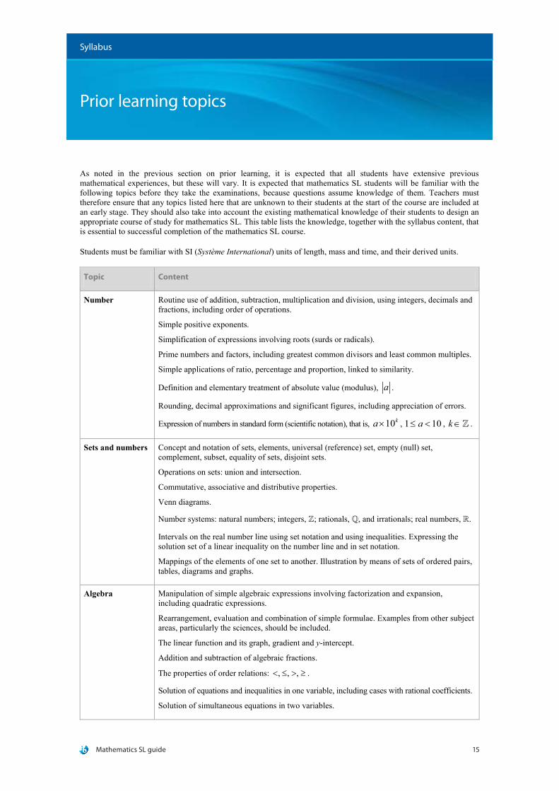
As noted in the previous section on prior learning, it is expected that all students have extensive previous mathematical experiences, but these will vary. It is expected that mathematics SL students will be familiar with the following topics before they take the examinations, because questions assume knowledge of them. Teachers must therefore ensure that any topics listed here that are unknown to their students at the start of the course are included at an early stage. They should also take into account the existing mathematical knowledge of their students to design an appropriate course of study for mathematics SL. This table lists the knowledge, together with the syllabus content, that is essential to successful completion of the mathematics SL course.
Students must be familiar with SI (Système International) units of length, mass and time, and their derived units.
Topic Content
Number Routine use of addition, subtraction, multiplication and division, using integers, decimals and fractions, including order of operations.
Simple positive exponents.
Simplification of expressions involving roots (surds or radicals).
Prime numbers and factors, including greatest common divisors and least common multiples.
Simple applications of ratio, percentage and proportion, linked to similarity.
Definition and elementary treatment of absolute value (modulus), a .
Rounding, decimal approximations and significant figures, including appreciation of errors.
Expression of numbers in standard form (scientific notation), that is, 10ka× , 1 10a≤ < , k∈ .
Sets and numbers Concept and notation of sets, elements, universal (reference) set, empty (null) set, complement, subset, equality of sets, disjoint sets.
Operations on sets: union and intersection.
Commutative, associative and distributive properties.
Venn diagrams.
Number systems: natural numbers; integers, ; rationals, , and irrationals; real numbers, .
Intervals on the real number line using set notation and using inequalities. Expressing the solution set of a linear inequality on the number line and in set notation.
Mappings of the elements of one set to another. Illustration by means of sets of ordered pairs, tables, diagrams and graphs.
Algebra Manipulation of simple algebraic expressions involving factorization and expansion, including quadratic expressions.
Rearrangement, evaluation and combination of simple formulae. Examples from other subject areas, particularly the sciences, should be included.
The linear function and its graph, gradient and y-intercept.
Addition and subtraction of algebraic fractions.
The properties of order relations: , , ,< ≤ > ≥ .
Solution of equations and inequalities in one variable, including cases with rational coefficients.
Solution of simultaneous equations in two variables.
Mathematics SL guide16
Prior learning topics
Topic Content
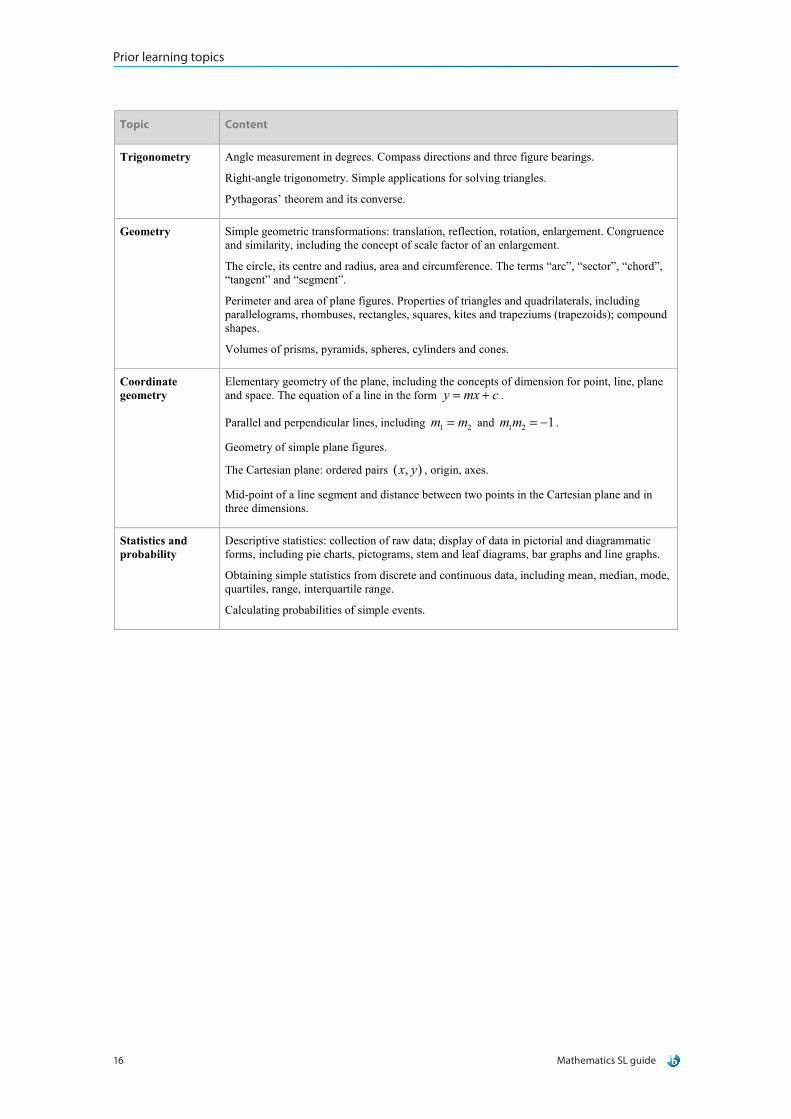
Trigonometry Angle measurement in degrees. Compass directions and three figure bearings.
Right-angle trigonometry. Simple applications for solving triangles.
Pythagoras’ theorem and its converse.
Geometry Simple geometric transformations: translation, reflection, rotation, enlargement. Congruence and similarity, including the concept of scale factor of an enlargement.
The circle, its centre and radius, area and circumference. The terms “arc”, “sector”, “chord”, “tangent” and “segment”.
Perimeter and area of plane figures. Properties of triangles and quadrilaterals, including parallelograms, rhombuses, rectangles, squares, kites and trapeziums (trapezoids); compound shapes.
Volumes of prisms, pyramids, spheres, cylinders and cones.
Coordinate geometry
Elementary geometry of the plane, including the concepts of dimension for point, line, plane and space. The equation of a line in the form y mx c= + .
Parallel and perpendicular lines, including 1 2m m= and 1 2 1m m = − .
Geometry of simple plane figures.
The Cartesian plane: ordered pairs ( , )x y , origin, axes.
Mid-point of a line segment and distance between two points in the Cartesian plane and in three dimensions.
Statistics and probability
Descriptive statistics: collection of raw data; display of data in pictorial and diagrammatic forms, including pie charts, pictograms, stem and leaf diagrams, bar graphs and line graphs.
Obtaining simple statistics from discrete and continuous data, including mean, median, mode, quartiles, range, interquartile range.
Calculating probabilities of simple events.
Mathem
atics SL guide17
Syllabus
Syllabus contentSyllabus content
Mathematics SL guide 1
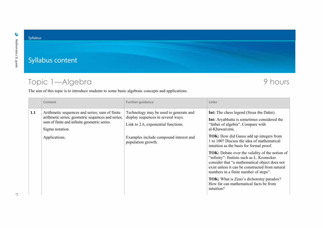
Topic 1—Algebra 9 hours The aim of this topic is to introduce students to some basic algebraic concepts and applications.
Content Further guidance Links
1.1 Arithmetic sequences and series; sum of finite arithmetic series; geometric sequences and series; sum of finite and infinite geometric series.
Sigma notation.
Technology may be used to generate and display sequences in several ways.
Link to 2.6, exponential functions.
Int: The chess legend (Sissa ibn Dahir).
Int: Aryabhatta is sometimes considered the “father of algebra”. Compare with al-Khawarizmi.
TOK: How did Gauss add up integers from 1 to 100? Discuss the idea of mathematical intuition as the basis for formal proof.
TOK: Debate over the validity of the notion of “infinity”: finitists such as L. Kronecker consider that “a mathematical object does not exist unless it can be constructed from natural numbers in a finite number of steps”.
TOK: What is Zeno’s dichotomy paradox? How far can mathematical facts be from intuition?
Applications. Examples include compound interest and population growth.
Mathem
atics SL guide18 Syllabus content
Syllabus content
Mathematics SL guide 2
Content Further guidance Links
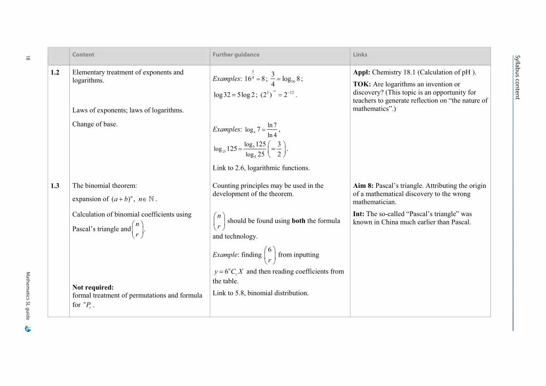
1.2 Elementary treatment of exponents and logarithms. Examples:
3416 8= ; 16
3 log 84= ;
log32 5log 2= ; 43 12(2 ) 2− −= .
Appl: Chemistry 18.1 (Calculation of pH ).
TOK: Are logarithms an invention or discovery? (This topic is an opportunity for teachers to generate reflection on “the nature of mathematics”.) Laws of exponents; laws of logarithms.
Change of base. Examples: 4
ln 7log
ln 47 = ,
255
5
loglog
log125 312525 2
= =
.
Link to 2.6, logarithmic functions.
1.3 The binomial theorem:
expansion of ( ) ,na b n+ ∈ .
Counting principles may be used in the development of the theorem.
Aim 8: Pascal’s triangle. Attributing the origin of a mathematical discovery to the wrong mathematician.
Int: The so-called “Pascal’s triangle” was known in China much earlier than Pascal.
Calculation of binomial coefficients using
Pascal’s triangle andnr
.
nr
should be found using both the formula
and technology.
Example: finding 6r
from inputting
6nry C X= and then reading coefficients from
the table.
Link to 5.8, binomial distribution. Not required: formal treatment of permutations and formula for n
rP .
Mathem
atics SL guide19
Syllabus contentSyllabus content
Mathematics SL guide 3
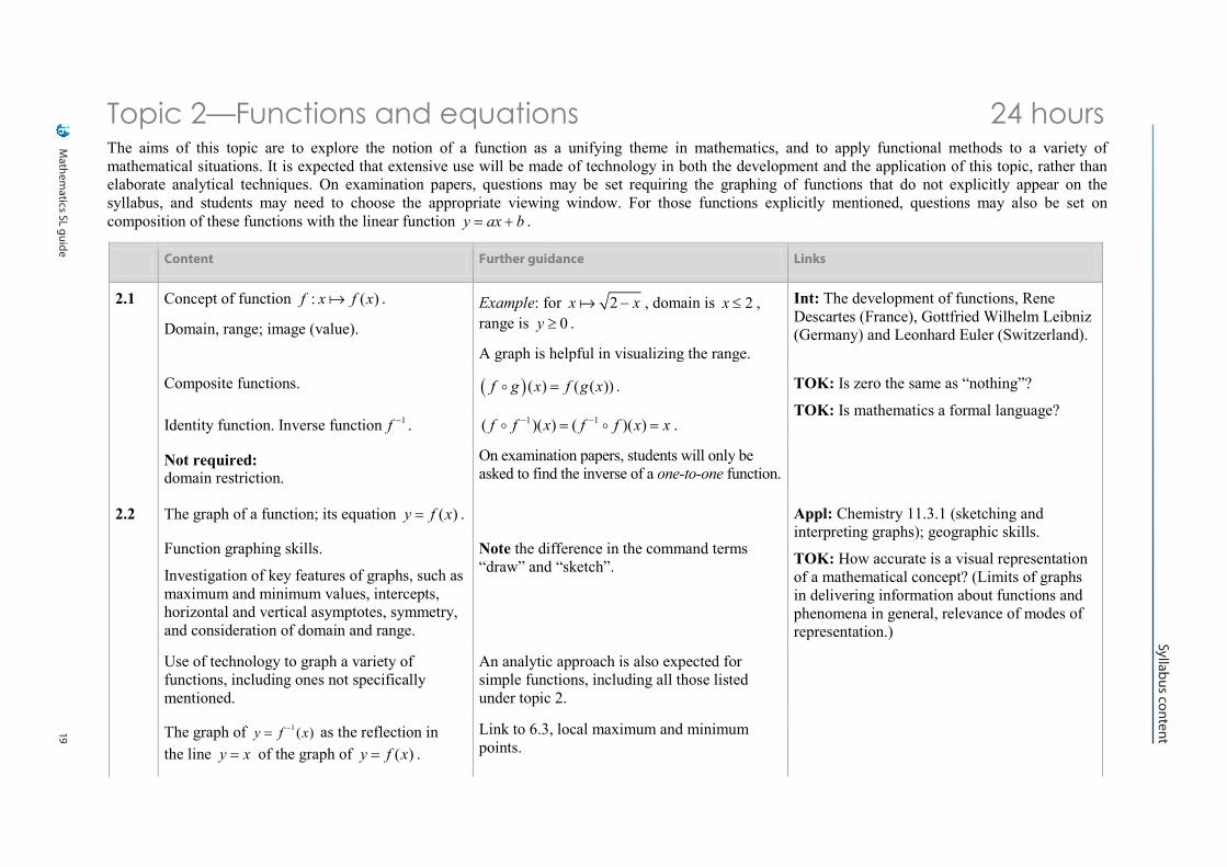
Topic 2—Functions and equations 24 hours The aims of this topic are to explore the notion of a function as a unifying theme in mathematics, and to apply functional methods to a variety of mathematical situations. It is expected that extensive use will be made of technology in both the development and the application of this topic, rather than elaborate analytical techniques. On examination papers, questions may be set requiring the graphing of functions that do not explicitly appear on the syllabus, and students may need to choose the appropriate viewing window. For those functions explicitly mentioned, questions may also be set on composition of these functions with the linear function y ax b= + .
Content Further guidance Links
2.1 Concept of function : ( )f x f x .
Domain, range; image (value). Example: for 2x x− , domain is 2x ≤ , range is 0y ≥ .
A graph is helpful in visualizing the range.
Int: The development of functions, Rene Descartes (France), Gottfried Wilhelm Leibniz (Germany) and Leonhard Euler (Switzerland).
Composite functions. ( )( ) ( ( ))f g x f g x= . TOK: Is zero the same as “nothing”?
TOK: Is mathematics a formal language? Identity function. Inverse function 1f − . 1 1( )( ) ( )( )f f x f f x x− −= = .
On examination papers, students will only be asked to find the inverse of a one-to-one function.
Not required: domain restriction.
2.2 The graph of a function; its equation ( )y f x= . Appl: Chemistry 11.3.1 (sketching and interpreting graphs); geographic skills.
TOK: How accurate is a visual representation of a mathematical concept? (Limits of graphs in delivering information about functions and phenomena in general, relevance of modes of representation.)
Function graphing skills.
Investigation of key features of graphs, such as maximum and minimum values, intercepts, horizontal and vertical asymptotes, symmetry, and consideration of domain and range.
Note the difference in the command terms “draw” and “sketch”.
Use of technology to graph a variety of functions, including ones not specifically mentioned.
An analytic approach is also expected for simple functions, including all those listed under topic 2.
The graph of 1 ( )y f x−= as the reflection in the line y x= of the graph of ( )y f x= .
Link to 6.3, local maximum and minimum points.
Mathem
atics SL guide20 Syllabus content
Syllabus content
Mathematics SL guide 4
Content Further guidance Links
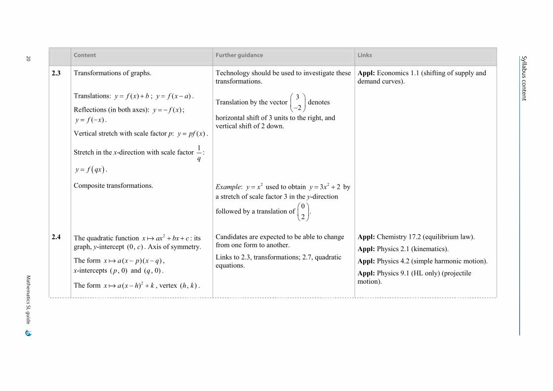
2.3 Transformations of graphs. Technology should be used to investigate these transformations.
Appl: Economics 1.1 (shifting of supply and demand curves).
Translations: ( )y f x b= + ; ( )y f x a= − .
Reflections (in both axes): ( )y f x= − ; ( )y f x= − .
Vertical stretch with scale factor p: ( )y pf x= .
Stretch in the x-direction with scale factor 1q
:
( )y f qx= .
Translation by the vector 32
−
denotes
horizontal shift of 3 units to the right, and vertical shift of 2 down.
Composite transformations. Example: 2y x= used to obtain 23 2y x= + by a stretch of scale factor 3 in the y-direction
followed by a translation of 02
.
2.4 The quadratic function 2x ax bx c+ + : its graph, y-intercept (0, )c . Axis of symmetry.
The form ( )( )x a x p x q− − , x-intercepts ( , 0)p and ( , 0)q .
The form 2( )x a x h k− + , vertex ( , )h k .
Candidates are expected to be able to change from one form to another.
Links to 2.3, transformations; 2.7, quadratic equations.
Appl: Chemistry 17.2 (equilibrium law).
Appl: Physics 2.1 (kinematics).
Appl: Physics 4.2 (simple harmonic motion).
Appl: Physics 9.1 (HL only) (projectile motion).
Mathem
atics SL guide21
Syllabus contentSyllabus content
Mathematics SL guide 5
Content Further guidance Links
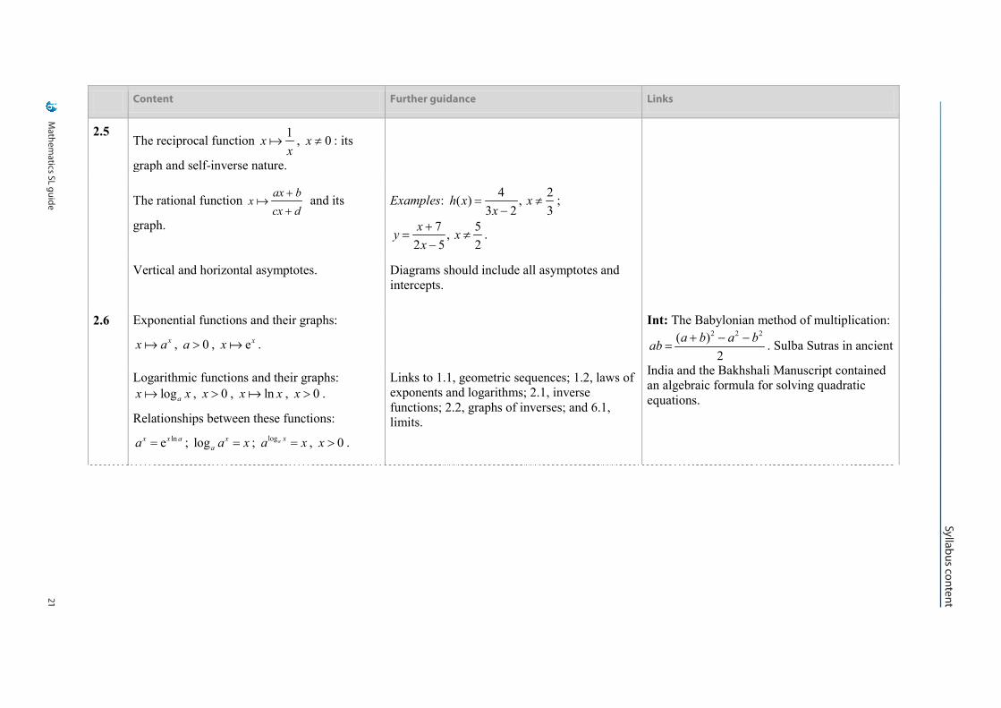
2.5 The reciprocal function 1x
x , 0x ≠ : its
graph and self-inverse nature.
The rational function ax bx
cx d+
+ and its
graph.
Examples: 4 2( ) , 3 2 3
h x xx
= ≠−
;
7 5, 2 5 2xy xx+
= ≠−
.
Vertical and horizontal asymptotes. Diagrams should include all asymptotes and intercepts.
2.6 Exponential functions and their graphs: xx a , 0a > , exx .
Int: The Babylonian method of multiplication: 2 2 2( )2
a b a bab + − −= . Sulba Sutras in ancient
India and the Bakhshali Manuscript contained an algebraic formula for solving quadratic equations.
Logarithmic functions and their graphs: logax x , 0x > , lnx x , 0x > .
Relationships between these functions: lnex x aa = ; log x
a a x= ; loga xa x= , 0x > .
Links to 1.1, geometric sequences; 1.2, laws of exponents and logarithms; 2.1, inverse functions; 2.2, graphs of inverses; and 6.1, limits.
Mathem
atics SL guide22 Syllabus content
Syllabus content
Mathematics SL guide 6
Content Further guidance Links
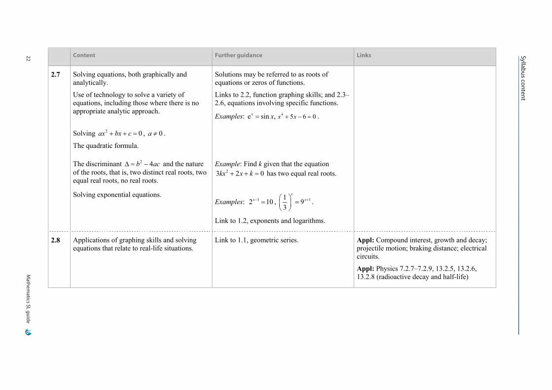
2.7 Solving equations, both graphically and analytically.
Use of technology to solve a variety of equations, including those where there is no appropriate analytic approach.
Solutions may be referred to as roots of equations or zeros of functions.
Links to 2.2, function graphing skills; and 2.3–2.6, equations involving specific functions.
Examples: 4 5 6 0e sin ,x x xx + − == .
Solving 2 0ax bx c+ + = , 0a ≠ .
The quadratic formula.
The discriminant 2 4b ac∆ = − and the nature of the roots, that is, two distinct real roots, two equal real roots, no real roots.
Example: Find k given that the equation 23 2 0kx x k+ + = has two equal real roots.
Solving exponential equations. Examples: 12 10x− = , 11 9
3
xx+ =
.
Link to 1.2, exponents and logarithms.
2.8 Applications of graphing skills and solving equations that relate to real-life situations.
Link to 1.1, geometric series. Appl: Compound interest, growth and decay; projectile motion; braking distance; electrical circuits.
Appl: Physics 7.2.7–7.2.9, 13.2.5, 13.2.6, 13.2.8 (radioactive decay and half-life)
Mathem
atics SL guide23
Syllabus contentSyllabus content
Mathematics SL guide 7
Topic 3—Circular functions and trigonometry 16 hours The aims of this topic are to explore the circular functions and to solve problems using trigonometry. On examination papers, radian measure should be assumed unless otherwise indicated.
Content Further guidance Links
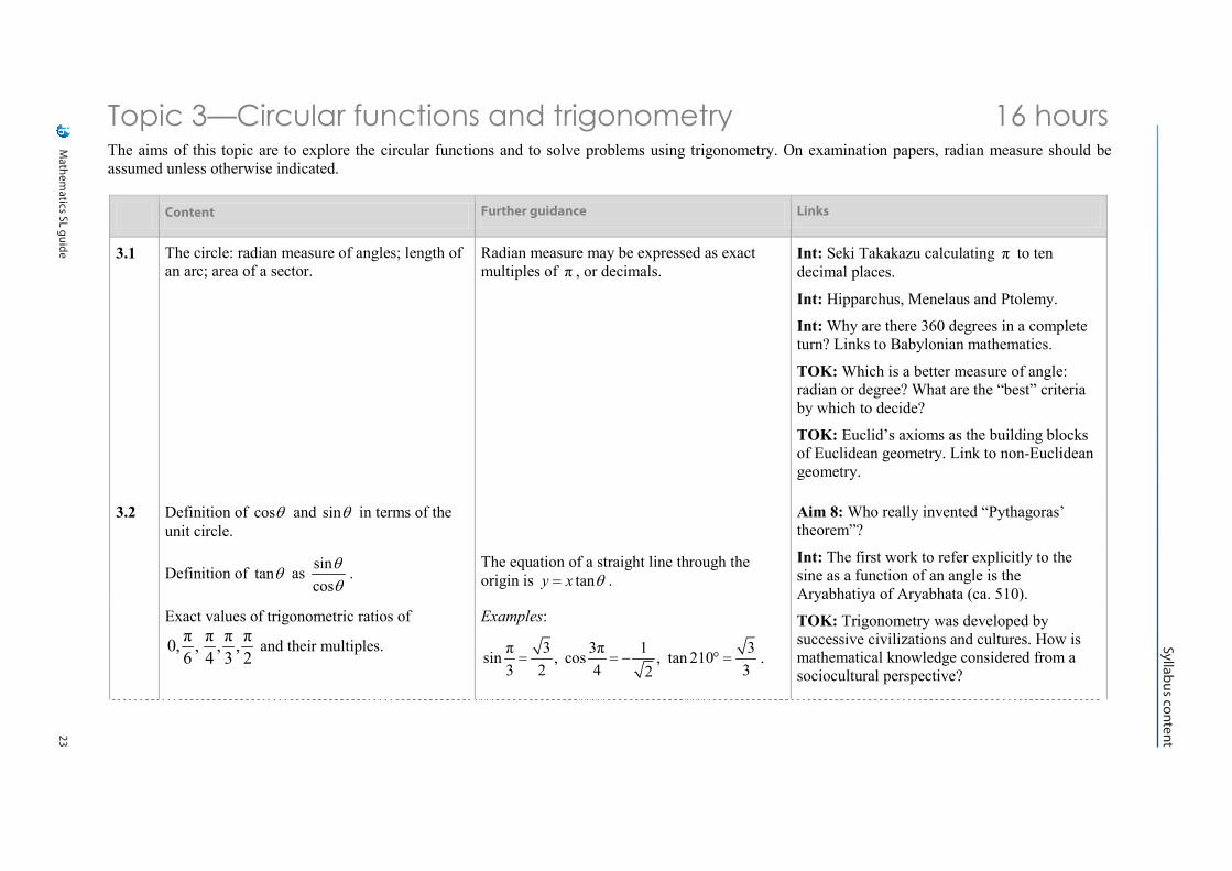
3.1 The circle: radian measure of angles; length of an arc; area of a sector.
Radian measure may be expressed as exact multiples of π , or decimals.
Int: Seki Takakazu calculating π to ten decimal places.
Int: Hipparchus, Menelaus and Ptolemy.
Int: Why are there 360 degrees in a complete turn? Links to Babylonian mathematics.
TOK: Which is a better measure of angle: radian or degree? What are the “best” criteria by which to decide?
TOK: Euclid’s axioms as the building blocks of Euclidean geometry. Link to non-Euclidean geometry.
3.2 Definition of cosθ and sinθ in terms of the unit circle.
Aim 8: Who really invented “Pythagoras’ theorem”?
Int: The first work to refer explicitly to the sine as a function of an angle is the Aryabhatiya of Aryabhata (ca. 510).
TOK: Trigonometry was developed by successive civilizations and cultures. How is mathematical knowledge considered from a sociocultural perspective?
Definition of tanθ as sincos
θθ
. The equation of a straight line through the origin is tany x θ= .
Exact values of trigonometric ratios of π π π π0, , , ,6 4 3 2
and their multiples.
Examples:
π 3 3π 1 3sin , cos , tan 2103 2 4 32= = − ° = .
Mathem
atics SL guide24 Syllabus content
Syllabus content
Mathematics SL guide 8
Content Further guidance Links
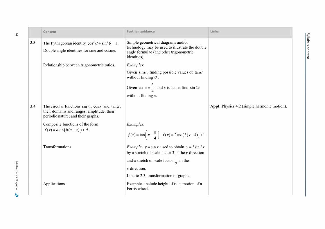
3.3 The Pythagorean identity 2 2cos sin 1θ θ+ = .
Double angle identities for sine and cosine.
Simple geometrical diagrams and/or technology may be used to illustrate the double angle formulae (and other trigonometric identities).
Relationship between trigonometric ratios. Examples:
Given sinθ , finding possible values of tanθ without finding θ .
Given 3cos4
x = , and x is acute, find sin 2x
without finding x.
3.4 The circular functions sin x , cos x and tan x : their domains and ranges; amplitude, their periodic nature; and their graphs.
Appl: Physics 4.2 (simple harmonic motion).
Composite functions of the form ( )( ) sin ( )f x a b x c d= + + .
Examples:
( ) tan4
f x x π = −
, ( )( ) 2cos 3( 4) 1f x x= − + .
Transformations. Example: siny x= used to obtain 3sin 2y x= by a stretch of scale factor 3 in the y-direction
and a stretch of scale factor 12
in the
x-direction.
Link to 2.3, transformation of graphs.
Applications. Examples include height of tide, motion of a Ferris wheel.
Mathem
atics SL guide25
Syllabus contentSyllabus content
Mathematics SL guide 9
Content Further guidance Links
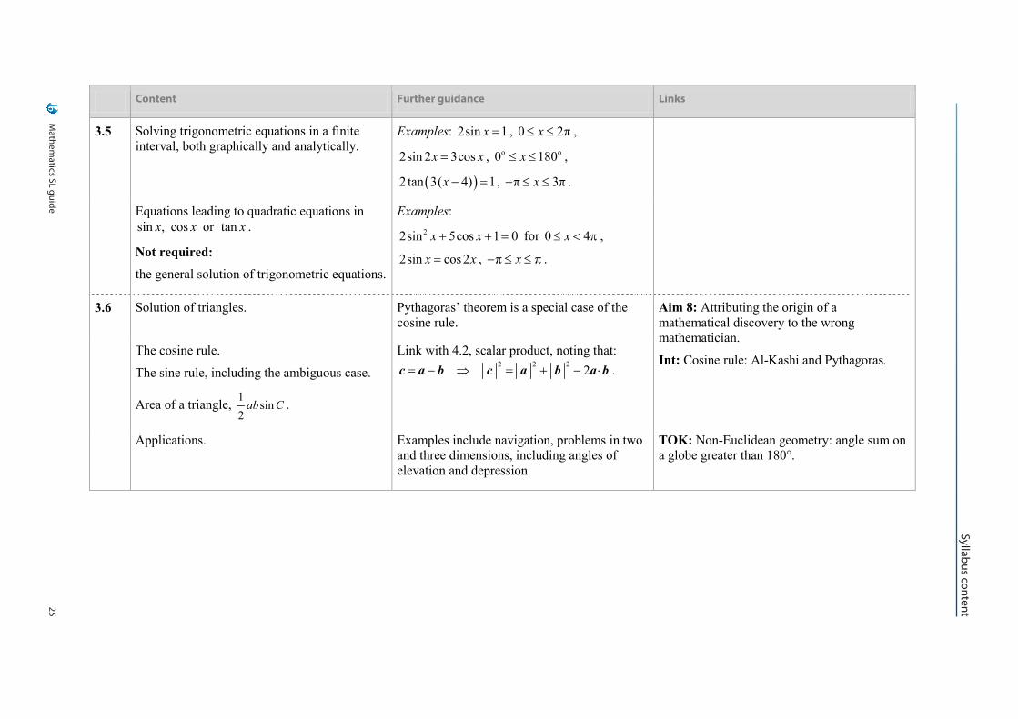
3.5 Solving trigonometric equations in a finite interval, both graphically and analytically.
Examples: 2sin 1x = , 0 2πx≤ ≤ ,
2sin 2 3cosx x= , o o0 180x≤ ≤ ,
( )2 tan 3( 4) 1x − = , π 3πx− ≤ ≤ .
Equations leading to quadratic equations in sin , cos or tanx x x .
Not required:
the general solution of trigonometric equations.
Examples: 22sin 5cos 1 0x x+ + = for 0 4x≤ < π ,
2sin cos2x x= , π πx− ≤ ≤ .
3.6 Solution of triangles. Pythagoras’ theorem is a special case of the cosine rule.
Aim 8: Attributing the origin of a mathematical discovery to the wrong mathematician.
Int: Cosine rule: Al-Kashi and Pythagoras. The cosine rule.
The sine rule, including the ambiguous case.
Area of a triangle, 1sin
2ab C .
Link with 4.2, scalar product, noting that: 2 2 2 2= − ⇒ = + − ⋅c a b c a b a b .
Applications. Examples include navigation, problems in two and three dimensions, including angles of elevation and depression.
TOK: Non-Euclidean geometry: angle sum on a globe greater than 180°.
Mathem
atics SL guide26 Syllabus content
Syllabus content
Mathematics SL guide 10
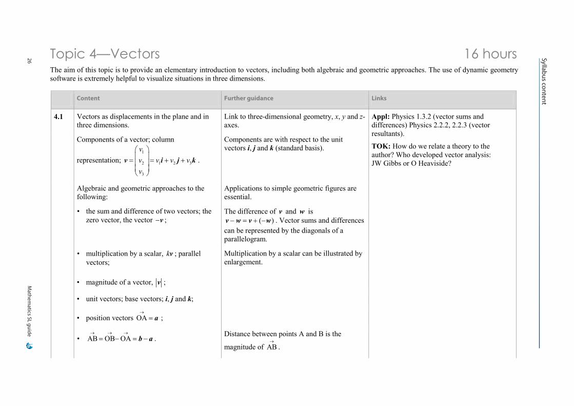
Topic 4—Vectors 16 hours The aim of this topic is to provide an elementary introduction to vectors, including both algebraic and geometric approaches. The use of dynamic geometry software is extremely helpful to visualize situations in three dimensions.
Content Further guidance Links
4.1 Vectors as displacements in the plane and in three dimensions.
Link to three-dimensional geometry, x, y and z-axes.
Appl: Physics 1.3.2 (vector sums and differences) Physics 2.2.2, 2.2.3 (vector resultants).
TOK: How do we relate a theory to the author? Who developed vector analysis: JW Gibbs or O Heaviside?
Components of a vector; column
representation; 1
2 1 2 3
3
vv v v vv
= = + +
v i j k .
Components are with respect to the unit vectors i, j and k (standard basis).
Algebraic and geometric approaches to the following:
Applications to simple geometric figures are essential.
• the sum and difference of two vectors; the zero vector, the vector −v ;
The difference of v and w is ( )− = + −v w v w . Vector sums and differences
can be represented by the diagonals of a parallelogram.
• multiplication by a scalar, kv ; parallel vectors;
Multiplication by a scalar can be illustrated by enlargement.
• magnitude of a vector, v ;
• unit vectors; base vectors; i, j and k;
• position vectors OA→
= a ;
• AB OB OA→ → →
= − = −b a . Distance between points A and B is the
magnitude of AB→
.
Mathem
atics SL guide27
Syllabus contentSyllabus content
Mathematics SL guide 11
Content Further guidance Links
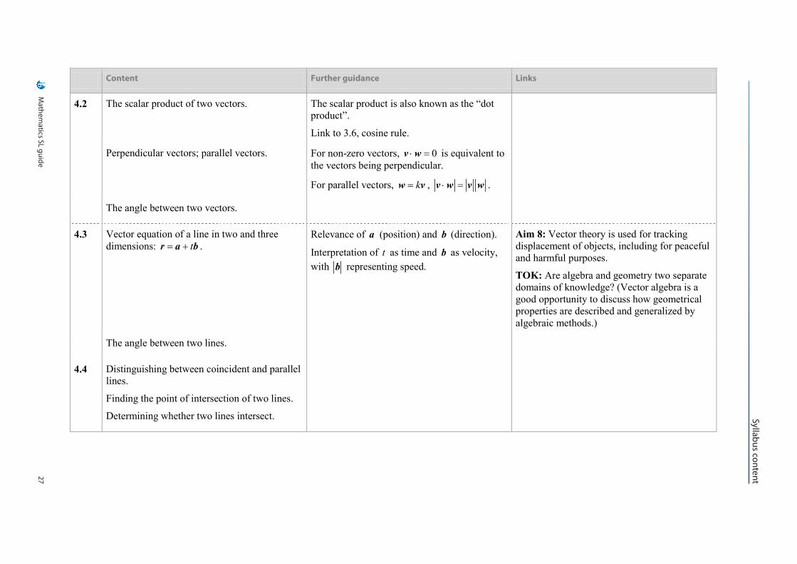
4.2 The scalar product of two vectors. The scalar product is also known as the “dot product”.
Link to 3.6, cosine rule.
Perpendicular vectors; parallel vectors. For non-zero vectors, 0⋅ =v w is equivalent to the vectors being perpendicular.
For parallel vectors, k=w v , ⋅ =v w v w .
The angle between two vectors.
4.3 Vector equation of a line in two and three dimensions: t= +r a b .
Relevance of a (position) and b (direction).
Interpretation of t as time and b as velocity, with b representing speed.
Aim 8: Vector theory is used for tracking displacement of objects, including for peaceful and harmful purposes.
TOK: Are algebra and geometry two separate domains of knowledge? (Vector algebra is a good opportunity to discuss how geometrical properties are described and generalized by algebraic methods.)
The angle between two lines.
4.4 Distinguishing between coincident and parallel lines.
Finding the point of intersection of two lines.
Determining whether two lines intersect.
Mathem
atics SL guide28 Syllabus content
Syllabus content
Mathematics SL guide 12
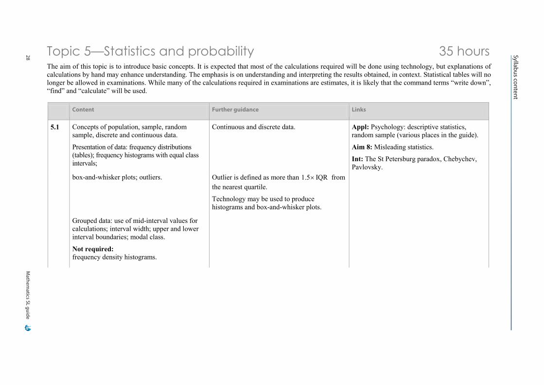
Topic 5—Statistics and probability 35 hours The aim of this topic is to introduce basic concepts. It is expected that most of the calculations required will be done using technology, but explanations of calculations by hand may enhance understanding. The emphasis is on understanding and interpreting the results obtained, in context. Statistical tables will no longer be allowed in examinations. While many of the calculations required in examinations are estimates, it is likely that the command terms “write down”, “find” and “calculate” will be used.
Content Further guidance Links
5.1 Concepts of population, sample, random sample, discrete and continuous data.
Presentation of data: frequency distributions (tables); frequency histograms with equal class intervals;
Continuous and discrete data. Appl: Psychology: descriptive statistics, random sample (various places in the guide).
Aim 8: Misleading statistics.
Int: The St Petersburg paradox, Chebychev, Pavlovsky.
box-and-whisker plots; outliers. Outlier is defined as more than 1.5 IQR× from the nearest quartile.
Technology may be used to produce histograms and box-and-whisker plots.
Grouped data: use of mid-interval values for calculations; interval width; upper and lower interval boundaries; modal class.
Not required: frequency density histograms.
Mathem
atics SL guide29
Syllabus contentSyllabus content
Mathematics SL guide 13
Content Further guidance Links
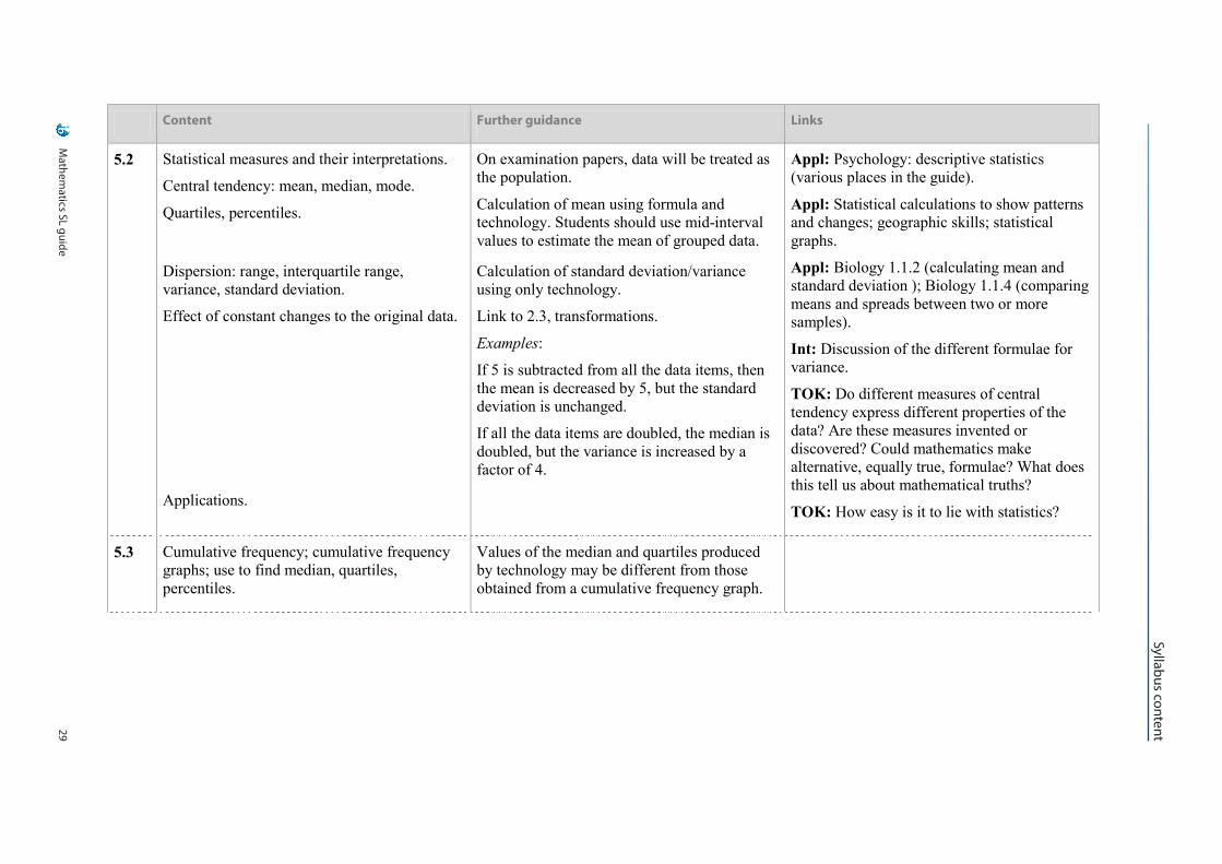
5.2 Statistical measures and their interpretations.
Central tendency: mean, median, mode.
Quartiles, percentiles.
On examination papers, data will be treated as the population.
Calculation of mean using formula and technology. Students should use mid-interval values to estimate the mean of grouped data.
Appl: Psychology: descriptive statistics (various places in the guide).
Appl: Statistical calculations to show patterns and changes; geographic skills; statistical graphs.
Appl: Biology 1.1.2 (calculating mean and standard deviation ); Biology 1.1.4 (comparing means and spreads between two or more samples).
Int: Discussion of the different formulae for variance.
TOK: Do different measures of central tendency express different properties of the data? Are these measures invented or discovered? Could mathematics make alternative, equally true, formulae? What does this tell us about mathematical truths?
TOK: How easy is it to lie with statistics?
Dispersion: range, interquartile range, variance, standard deviation.
Effect of constant changes to the original data.
Calculation of standard deviation/variance using only technology.
Link to 2.3, transformations.
Examples:
If 5 is subtracted from all the data items, then the mean is decreased by 5, but the standard deviation is unchanged.
If all the data items are doubled, the median is doubled, but the variance is increased by a factor of 4.
Applications.
5.3 Cumulative frequency; cumulative frequency graphs; use to find median, quartiles, percentiles.
Values of the median and quartiles produced by technology may be different from those obtained from a cumulative frequency graph.
Mathem
atics SL guide30 Syllabus content
Syllabus content
Mathematics SL guide 14
Content Further guidance Links
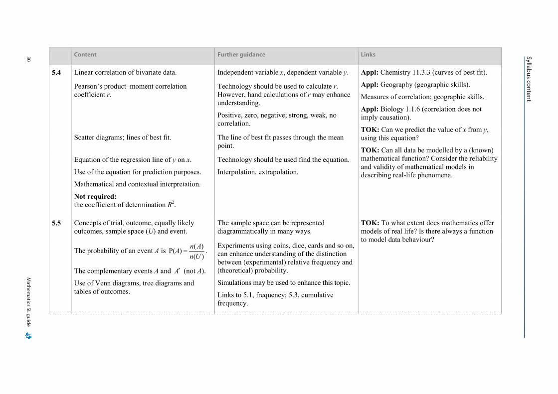
5.4 Linear correlation of bivariate data. Independent variable x, dependent variable y. Appl: Chemistry 11.3.3 (curves of best fit).
Appl: Geography (geographic skills).
Measures of correlation; geographic skills.
Appl: Biology 1.1.6 (correlation does not imply causation).
TOK: Can we predict the value of x from y, using this equation?
TOK: Can all data be modelled by a (known) mathematical function? Consider the reliability and validity of mathematical models in describing real-life phenomena.
Pearson’s product–moment correlation coefficient r.
Technology should be used to calculate r. However, hand calculations of r may enhance understanding.
Positive, zero, negative; strong, weak, no correlation.
Scatter diagrams; lines of best fit. The line of best fit passes through the mean point.
Equation of the regression line of y on x.
Use of the equation for prediction purposes.
Mathematical and contextual interpretation.
Not required: the coefficient of determination R2.
Technology should be used find the equation.
Interpolation, extrapolation.
5.5 Concepts of trial, outcome, equally likely outcomes, sample space (U) and event.
The sample space can be represented diagrammatically in many ways.
TOK: To what extent does mathematics offer models of real life? Is there always a function to model data behaviour?
The probability of an event A is ( )P( )( )
n AAn U
= .
The complementary events A and A′ (not A).
Use of Venn diagrams, tree diagrams and tables of outcomes.
Experiments using coins, dice, cards and so on, can enhance understanding of the distinction between (experimental) relative frequency and (theoretical) probability.
Simulations may be used to enhance this topic.
Links to 5.1, frequency; 5.3, cumulative frequency.
Mathem
atics SL guide31
Syllabus contentSyllabus content
Mathematics SL guide 15
Content Further guidance Links
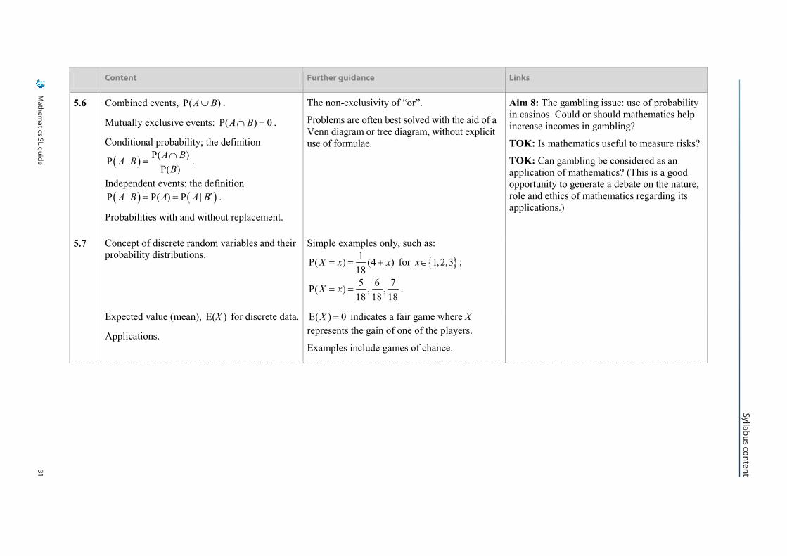
5.6 Combined events, P( )A B∪ .
Mutually exclusive events: P( ) 0A B∩ = .
Conditional probability; the definition
( ) P( )P |P( )A BA B
B∩
= .
Independent events; the definition ( ) ( )P | P( ) P |A B A A B′= = .
Probabilities with and without replacement.
The non-exclusivity of “or”.
Problems are often best solved with the aid of a Venn diagram or tree diagram, without explicit use of formulae.
Aim 8: The gambling issue: use of probability in casinos. Could or should mathematics help increase incomes in gambling?
TOK: Is mathematics useful to measure risks?
TOK: Can gambling be considered as an application of mathematics? (This is a good opportunity to generate a debate on the nature, role and ethics of mathematics regarding its applications.)
5.7 Concept of discrete random variables and their probability distributions.
Simple examples only, such as: 1P( ) (4 )
18X x x= = + for { }1,2,3x∈ ;
5 6 7P( ) , ,18 18 18
X x= = .
Expected value (mean), E( )X for discrete data.
Applications.
E( ) 0X = indicates a fair game where X represents the gain of one of the players.
Examples include games of chance.
Mathem
atics SL guide32 Syllabus content
Syllabus content
Mathematics SL guide 16
Content Further guidance Links
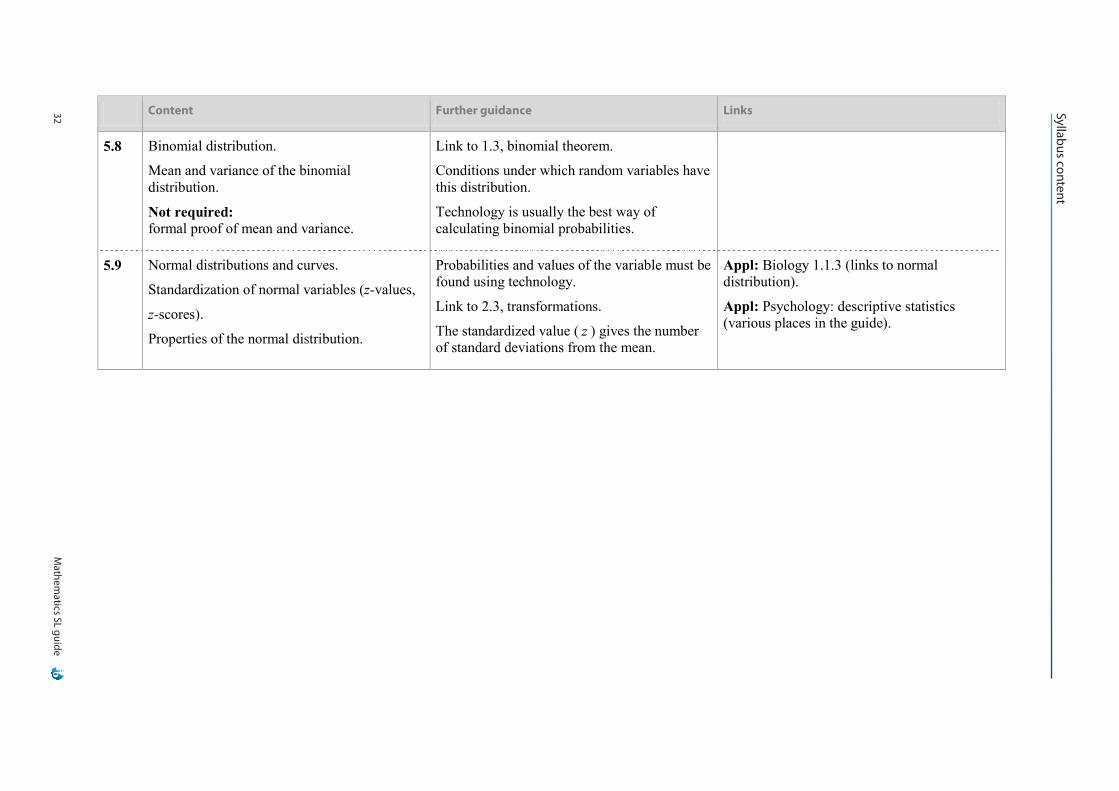
5.8 Binomial distribution.
Mean and variance of the binomial distribution.
Not required: formal proof of mean and variance.
Link to 1.3, binomial theorem.
Conditions under which random variables have this distribution.
Technology is usually the best way of calculating binomial probabilities.
5.9 Normal distributions and curves.
Standardization of normal variables (z-values,
z-scores).
Properties of the normal distribution.
Probabilities and values of the variable must be found using technology.
Link to 2.3, transformations.
The standardized value ( z ) gives the number of standard deviations from the mean.
Appl: Biology 1.1.3 (links to normal distribution).
Appl: Psychology: descriptive statistics (various places in the guide).
Mathem
atics SL guide33
Syllabus contentSyllabus content
Mathematics SL guide 17
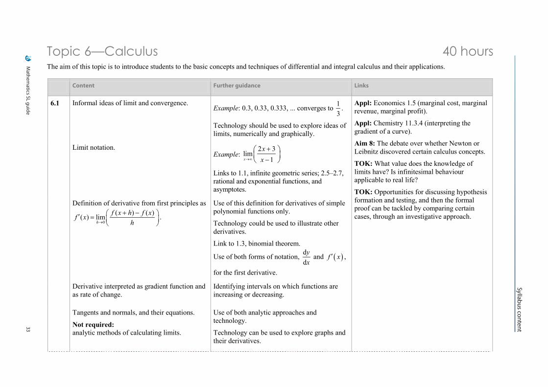
Topic 6—Calculus 40 hours The aim of this topic is to introduce students to the basic concepts and techniques of differential and integral calculus and their applications.
Content Further guidance Links
6.1 Informal ideas of limit and convergence. Example: 0.3, 0.33, 0.333, ... converges to 1
3.
Technology should be used to explore ideas of limits, numerically and graphically.
Appl: Economics 1.5 (marginal cost, marginal revenue, marginal profit).
Appl: Chemistry 11.3.4 (interpreting the gradient of a curve).
Aim 8: The debate over whether Newton or Leibnitz discovered certain calculus concepts.
TOK: What value does the knowledge of limits have? Is infinitesimal behaviour applicable to real life?
TOK: Opportunities for discussing hypothesis formation and testing, and then the formal proof can be tackled by comparing certain cases, through an investigative approach.
Limit notation. Example:
2 3lim
1x
xx→∞
+
−
Links to 1.1, infinite geometric series; 2.5–2.7, rational and exponential functions, and asymptotes.
Definition of derivative from first principles as
0
( ) ( )( ) limh
f x h f xf xh→
+ − ′ =
.
Use of this definition for derivatives of simple polynomial functions only.
Technology could be used to illustrate other derivatives.
Link to 1.3, binomial theorem.
Use of both forms of notation, ddyx
and ( )f x′ ,
for the first derivative.
Derivative interpreted as gradient function and as rate of change.
Identifying intervals on which functions are increasing or decreasing.
Tangents and normals, and their equations.
Not required: analytic methods of calculating limits.
Use of both analytic approaches and technology.
Technology can be used to explore graphs and their derivatives.
Mathem
atics SL guide34 Syllabus content
Syllabus content
Mathematics SL guide 18
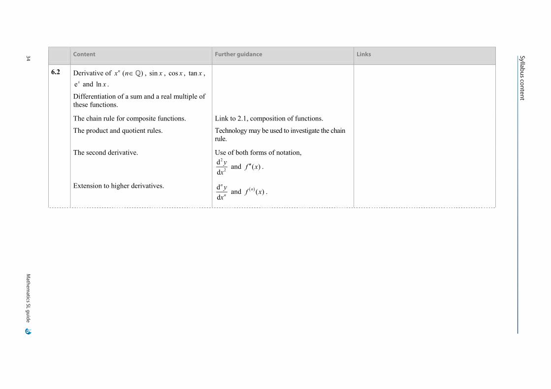
Content Further guidance Links
6.2 Derivative of ( )nx n∈ , sin x , cos x , tan x , ex and ln x .
Differentiation of a sum and a real multiple of these functions.
The chain rule for composite functions.
The product and quotient rules.
Link to 2.1, composition of functions.
Technology may be used to investigate the chain rule.
The second derivative. Use of both forms of notation, 2
2
dd
yx
and ( )f x′′ .
Extension to higher derivatives. dd
n
n
yx
and ( ) ( )nf x .
Mathem
atics SL guide35
Syllabus contentSyllabus content
Mathematics SL guide 19
Content Further guidance Links
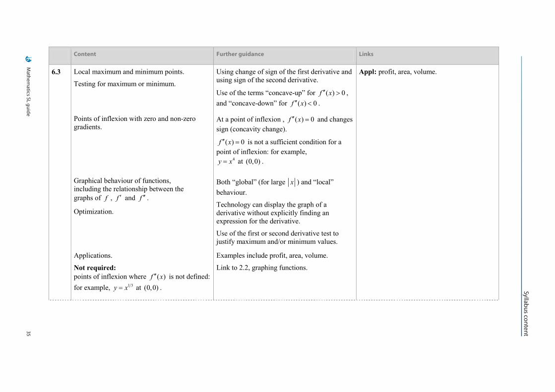
6.3 Local maximum and minimum points.
Testing for maximum or minimum.
Using change of sign of the first derivative and using sign of the second derivative.
Use of the terms “concave-up” for ( ) 0f x′′ > , and “concave-down” for ( ) 0f x′′ < .
Appl: profit, area, volume.
Points of inflexion with zero and non-zero gradients.
At a point of inflexion , ( ) 0f x′′ = and changes sign (concavity change).
( ) 0f x′′ = is not a sufficient condition for a point of inflexion: for example,
4y x= at (0,0) .
Graphical behaviour of functions, including the relationship between the graphs of f , f ′ and f ′′ .
Optimization.
Both “global” (for large x ) and “local” behaviour.
Technology can display the graph of a derivative without explicitly finding an expression for the derivative.
Use of the first or second derivative test to justify maximum and/or minimum values.
Applications.
Not required: points of inflexion where ( )f x′′ is not defined: for example, 1 3y x= at (0,0) .
Examples include profit, area, volume.
Link to 2.2, graphing functions.
Mathem
atics SL guide36 Syllabus content
Syllabus content
Mathematics SL guide 20
Content Further guidance Links
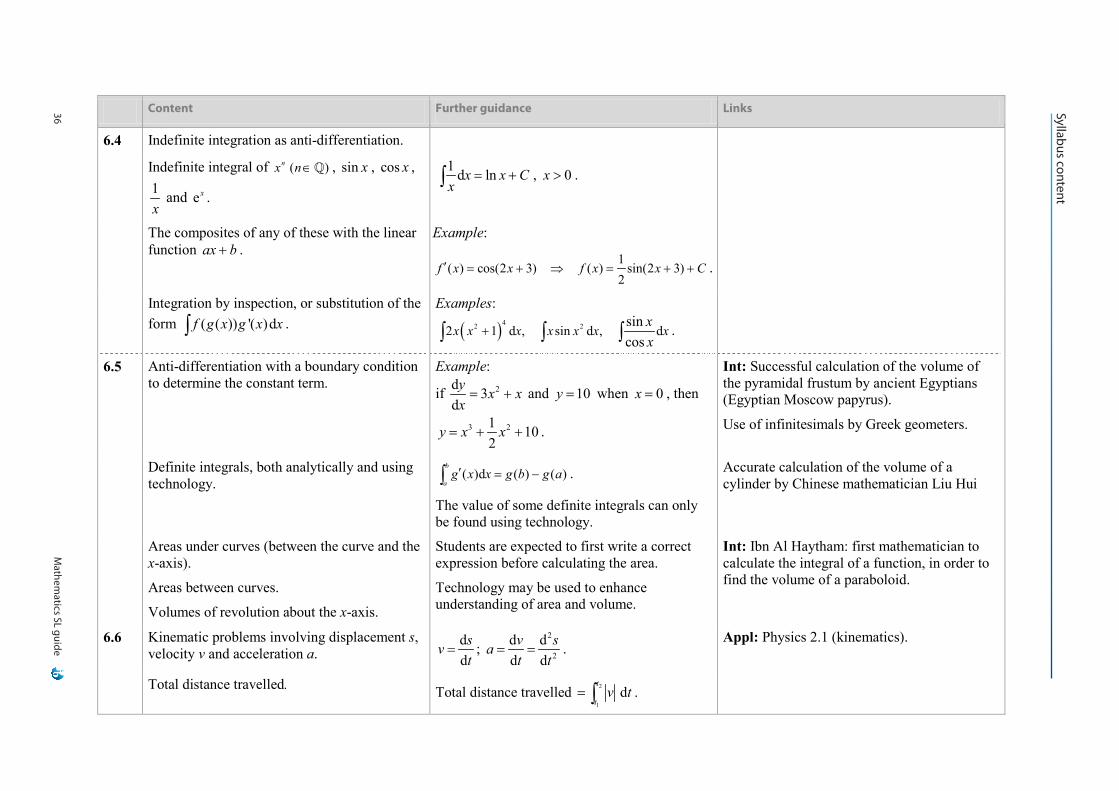
6.4 Indefinite integration as anti-differentiation.
Indefinite integral of ( )nx n∈ , sin x , cos x , 1x
and ex .
1 d lnx x Cx
= +∫ , 0x > .
The composites of any of these with the linear function ax b+ .
Example:
1( ) cos(2 3) ( ) sin(2 3)
2f x x f x x C′ = + ⇒ = + + .
Integration by inspection, or substitution of the form ( ( )) '( )df g x g x x∫ .
Examples:
( )42 22 1 d , sin d , dsincos
x x x x x x xxx
+∫ ∫ ∫ .
6.5 Anti-differentiation with a boundary condition to determine the constant term.
Example:
if 2d 3dy x xx= + and 10y = when 0x = , then
3 21 102
y x x= + + .
Int: Successful calculation of the volume of the pyramidal frustum by ancient Egyptians (Egyptian Moscow papyrus).
Use of infinitesimals by Greek geometers.
Definite integrals, both analytically and using technology.
( )d ( ) ( )b
ag x x g b g a′ = −∫ .
The value of some definite integrals can only be found using technology.
Accurate calculation of the volume of a cylinder by Chinese mathematician Liu Hui
Areas under curves (between the curve and the x-axis).
Areas between curves.
Volumes of revolution about the x-axis.
Students are expected to first write a correct expression before calculating the area.
Technology may be used to enhance understanding of area and volume.
Int: Ibn Al Haytham: first mathematician to calculate the integral of a function, in order to find the volume of a paraboloid.
6.6 Kinematic problems involving displacement s, velocity v and acceleration a.
ddsvt
= ; 2
2
d dd dv sat t
= = . Appl: Physics 2.1 (kinematics).
Total distance travelled. Total distance travelled 2
1
dt
tv t= ∫ .
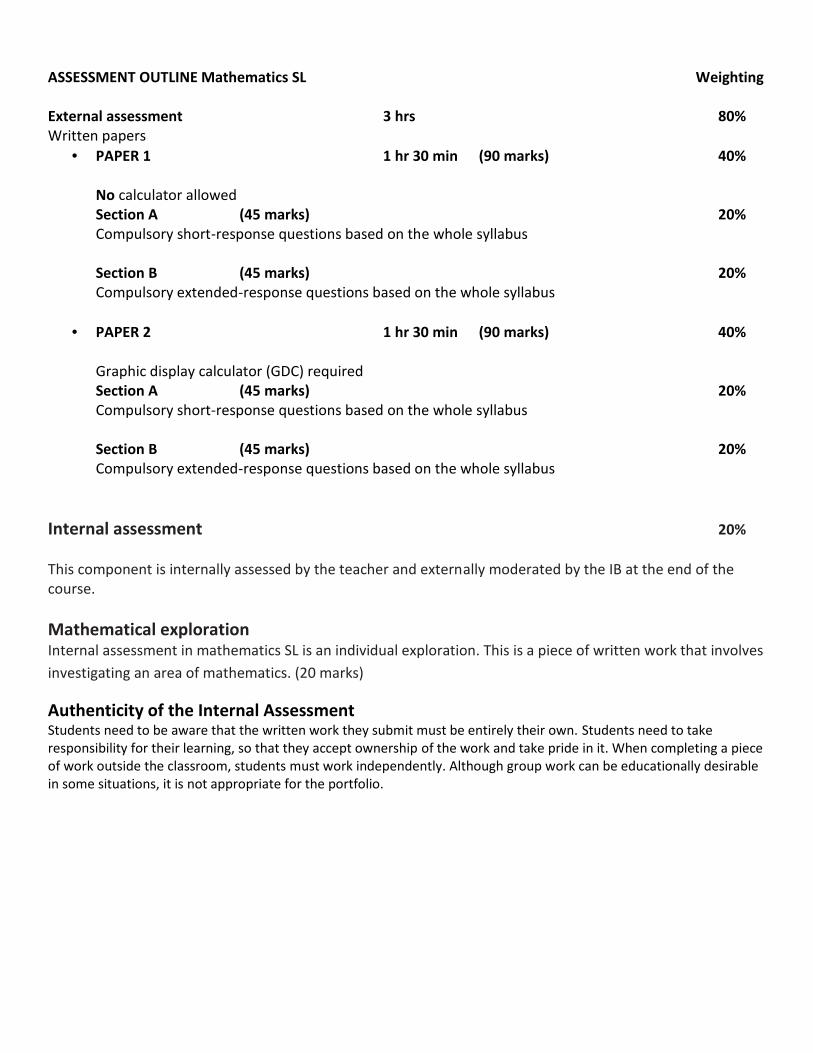
ASSESSMENT OUTLINE Mathematics SL Weighting
External assessment 3 hrs 80%Written papers
PAPER 1 1 hr 30 min (90 marks) 40%
No calculator allowedSection A (45 marks) 20%Compulsory short-response questions based on the whole syllabus
Section B (45 marks) 20%Compulsory extended-response questions based on the whole syllabus
PAPER 2 1 hr 30 min (90 marks) 40%
Graphic display calculator (GDC) requiredSection A (45 marks) 20%Compulsory short-response questions based on the whole syllabus
Section B (45 marks) 20%Compulsory extended-response questions based on the whole syllabus
Internal assessment 20%
This component is internally assessed by the teacher and externally moderated by the IB at the end of thecourse.
Mathematical explorationInternal assessment in mathematics SL is an individual exploration. This is a piece of written work that involvesinvestigating an area of mathematics. (20 marks)
Authenticity of the Internal AssessmentStudents need to be aware that the written work they submit must be entirely their own. Students need to takeresponsibility for their learning, so that they accept ownership of the work and take pride in it. When completing a pieceof work outside the classroom, students must work independently. Although group work can be educationally desirablein some situations, it is not appropriate for the portfolio.
Mathematics SL guide 47
Internal assessment
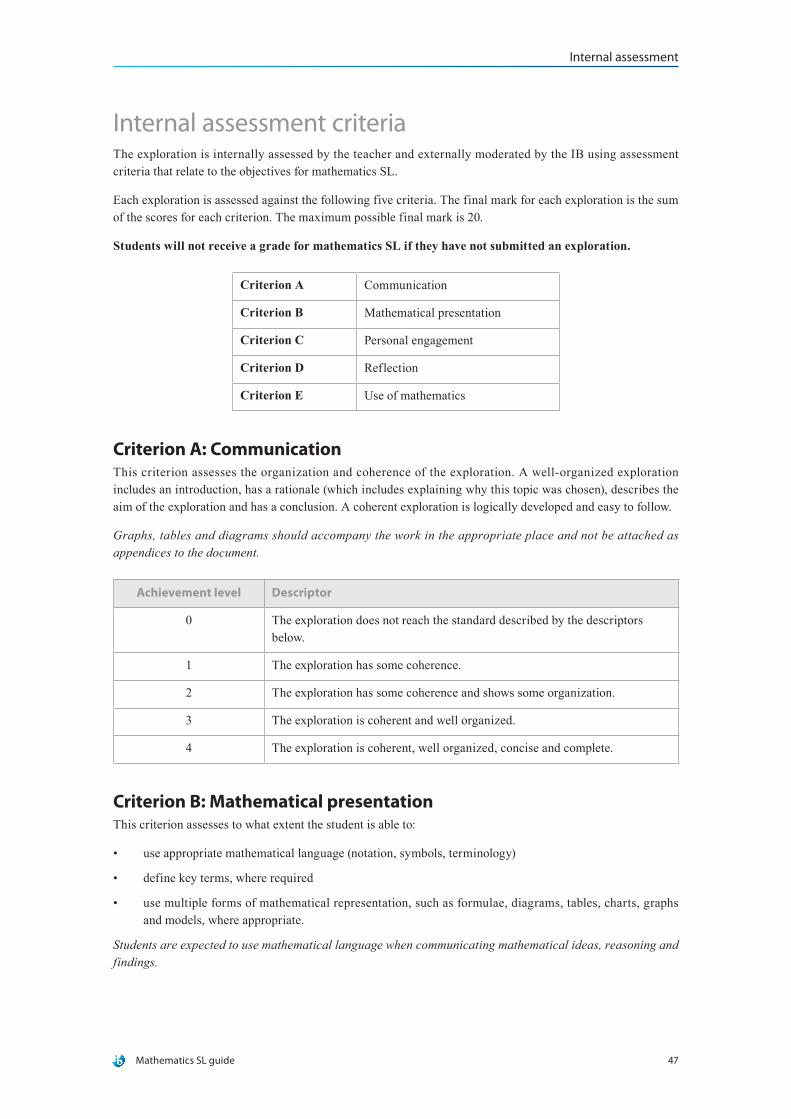
Internal assessment criteriaThe exploration is internally assessed by the teacher and externally moderated by the IB using assessment criteria that relate to the objectives for mathematics SL.
Each exploration is assessed against the following five criteria. The final mark for each exploration is the sum of the scores for each criterion. The maximum possible final mark is 20.
Students will not receive a grade for mathematics SL if they have not submitted an exploration.
Criterion A Communication
Criterion B Mathematical presentation
Criterion C Personal engagement
Criterion D Reflection
Criterion E Use of mathematics
Criterion A: CommunicationThis criterion assesses the organization and coherence of the exploration. A well-organized exploration includes an introduction, has a rationale (which includes explaining why this topic was chosen), describes the aim of the exploration and has a conclusion. A coherent exploration is logically developed and easy to follow.
Graphs, tables and diagrams should accompany the work in the appropriate place and not be attached as appendices to the document.
Achievement level Descriptor
0 The exploration does not reach the standard described by the descriptors below.
1 The exploration has some coherence.
2 The exploration has some coherence and shows some organization.
3 The exploration is coherent and well organized.
4 The exploration is coherent, well organized, concise and complete.
Criterion B: Mathematical presentationThis criterion assesses to what extent the student is able to:
• use appropriate mathematical language (notation, symbols, terminology)
• define key terms, where required
• use multiple forms of mathematical representation, such as formulae, diagrams, tables, charts, graphs and models, where appropriate.
Students are expected to use mathematical language when communicating mathematical ideas, reasoning and findings.
Mathematics SL guide48
Internal assessment
Students are encouraged to choose and use appropriate ICT tools such as graphic display calculators, screenshots, graphing, spreadsheets, databases, drawing and word-processing software, as appropriate, to enhance mathematical communication.
Achievement level Descriptor
0 The exploration does not reach the standard described by the descriptors below.
1 There is some appropriate mathematical presentation.
2 The mathematical presentation is mostly appropriate.
3 The mathematical presentation is appropriate throughout.
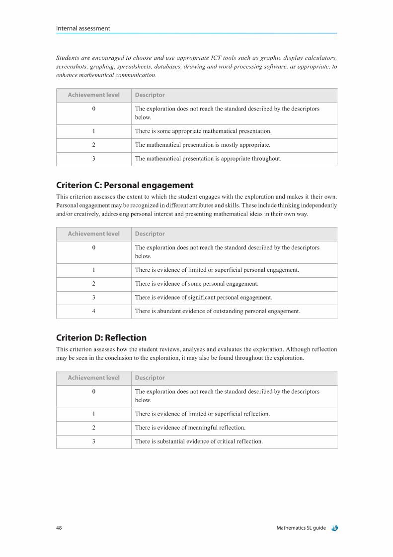
Criterion C: Personal engagementThis criterion assesses the extent to which the student engages with the exploration and makes it their own. Personal engagement may be recognized in different attributes and skills. These include thinking independently and/or creatively, addressing personal interest and presenting mathematical ideas in their own way.
Achievement level Descriptor
0 The exploration does not reach the standard described by the descriptors below.
1 There is evidence of limited or superficial personal engagement.
2 There is evidence of some personal engagement.
3 There is evidence of significant personal engagement.
4 There is abundant evidence of outstanding personal engagement.
Criterion D: ReflectionThis criterion assesses how the student reviews, analyses and evaluates the exploration. Although reflection may be seen in the conclusion to the exploration, it may also be found throughout the exploration.
Achievement level Descriptor
0 The exploration does not reach the standard described by the descriptors below.
1 There is evidence of limited or superficial reflection.
2 There is evidence of meaningful reflection.
3 There is substantial evidence of critical reflection.

Mathematics SL guide 49
Internal assessment
Criterion E: Use of mathematicsThis criterion assesses to what extent students use mathematics in the exploration.
Students are expected to produce work that is commensurate with the level of the course. The mathematics explored should either be part of the syllabus, or at a similar level or beyond. It should not be completely based on mathematics listed in the prior learning. If the level of mathematics is not commensurate with the level of the course, a maximum of two marks can be awarded for this criterion.
The mathematics can be regarded as correct even if there are occasional minor errors as long as they do not detract from the flow of the mathematics or lead to an unreasonable outcome.
Achievement level Descriptor
0 The exploration does not reach the standard described by the descriptors below.
1 Some relevant mathematics is used.
2 Some relevant mathematics is used. Limited understanding is demonstrated.
3 Relevant mathematics commensurate with the level of the course is used. Limited understanding is demonstrated.
4 Relevant mathematics commensurate with the level of the course is used. The mathematics explored is partially correct. Some knowledge and understanding are demonstrated.
5 Relevant mathematics commensurate with the level of the course is used. The mathematics explored is mostly correct. Good knowledge and understanding are demonstrated.
6 Relevant mathematics commensurate with the level of the course is used. The mathematics explored is correct. Thorough knowledge and understanding are demonstrated.

Resources:1. Mathematics standard Level for the IB Diploma by Smedly and Wiseman ( Oxford University Press )2. Mathematics Standard Level Published by IBDP Press3. Higher Level Mathematics for the IB Diploma by (Pearson Baccalaureate)4. Extended Mathematics for IGCSE by David Rayner5. Additional Mathematics by JF Talbert and HH Heng6. IBDP Math Question Bank

Mathematics SL and HL teacher support material 1
Example 2: Student work
Proving Euler’s Totient Theorem
M ATHS COURSEWORK
Proving Euler’s Totient Theorem

Mathematics SL and HL teacher support material 2
Example 2: Student work
Proving Euler’s Totient Theorem
TA B L E O F C O N T E N T S
Maths Coursework 3
Introduction 3
The Theorem 3
Euler’s Totient Function 3
Fermat’s Little Theorem 4
Proving Fermat’s Little Theorem 5
Proving Euler’s Totient Theorem 6
Applications 7
Conclusion 7
Mathematics SL and HL teacher support material 3
Example 2: Student work
Proving Euler’s Totient Theorem
M ATHS COURSEWORK
Proving Euler’s Totient Theorem
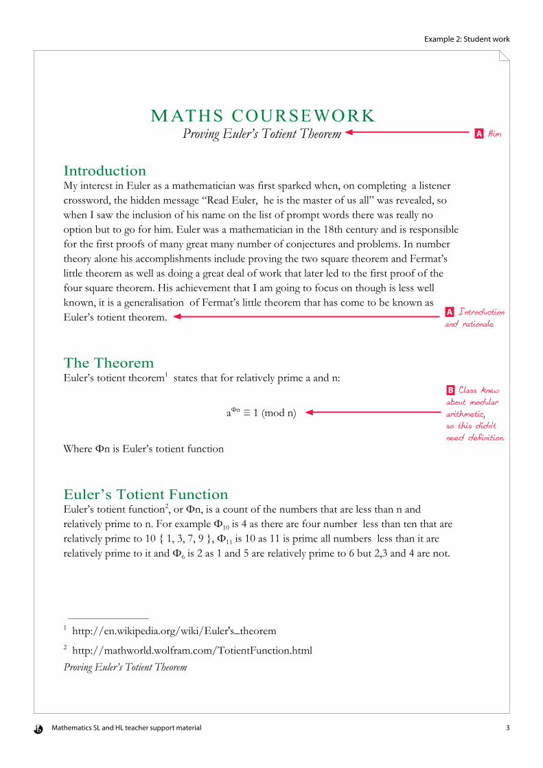
Introduction My interest in Euler as a mathematician was first sparked when, on completing a listener crossword, the hidden message “Read Euler, he is the master of us all” was revealed, so when I saw the inclusion of his name on the list of prompt words there was really no option but to go for him. Euler was a mathematician in the 18th century and is responsible for the first proofs of many great many number of conjectures and problems. In number theory alone his accomplishments include proving the two square theorem and Fermat’s little theorem as well as doing a great deal of work that later led to the first proof of the four square theorem. His achievement that I am going to focus on though is less well known, it is a generalisation of Fermat’s little theorem that has come to be known as Euler’s totient theorem.
The Theorem Euler’s totient theorem1 states that for relatively prime a and n:
aΦn ≡ 1 (mod n)
Where Φn is Euler’s totient function
Euler’s Totient Function Euler’s totient function2, or Φn, is a count of the numbers that are less than n and relatively prime to n. For example Φ10 is 4 as there are four number less than ten that are relatively prime to 10 { 1, 3, 7, 9 }, Φ11 is 10 as 11 is prime all numbers less than it are relatively prime to it and Φ6 is 2 as 1 and 5 are relatively prime to 6 but 2,3 and 4 are not.
1 http://en.wikipedia.org/wiki/Euler's_theorem 2 http://mathworld.wolfram.com/TotientFunction.html
A Aim
A Introduction and rationale
B Class knew about modular arithmetic, so this didn't need definition.
Mathematics SL and HL teacher support material 4
Example 2: Student work
Proving Euler’s Totient Theorem
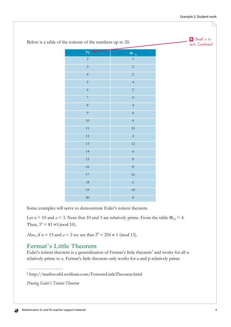
Below is a table of the totients of the numbers up to 20.
N Φ N 2 1
3 2
4 2
5 4
6 2
7 6
8 4
9 6
10 4
11 10
12 4
13 12
14 6
15 8
16 8
17 16
18 6
19 18
20 8
Some examples will serve to demonstrate Euler’s totient theorem.
Let n = 10 and a = 3. Note that 10 and 3 are relatively prime. From the table Φ10 = 4. Then, 34 = 81 ≡1(mod 10).
Also, if n = 15 and a = 2 we see that 28 = 256 ≡ 1 (mod 15).
Fermat’s Little Theorem Euler’s totient theorem is a generalisation of Fermat’s little theorem3 and works for all n relatively prime to a. Fermat’s little theorem only works for a and p relatively prime
3 http://mathworld.wolfram.com/FermatsLittleTheorem.html
B Small n in text. Condoned
Mathematics SL and HL teacher support material 5
Example 2: Student work
Proving Euler’s Totient Theorem
where p is itself prime and states:
ap ≡ a (mod p)
or
ap-1 ≡ 1 (mod p)
It is immediately apparent that this fits in with Euler’s totient theorem for primes p, as we have seen Φp, where p is a prime, is always p-1.
As an introduction to Euler’s totient theorem I shall prove Fermat’s little theorem.
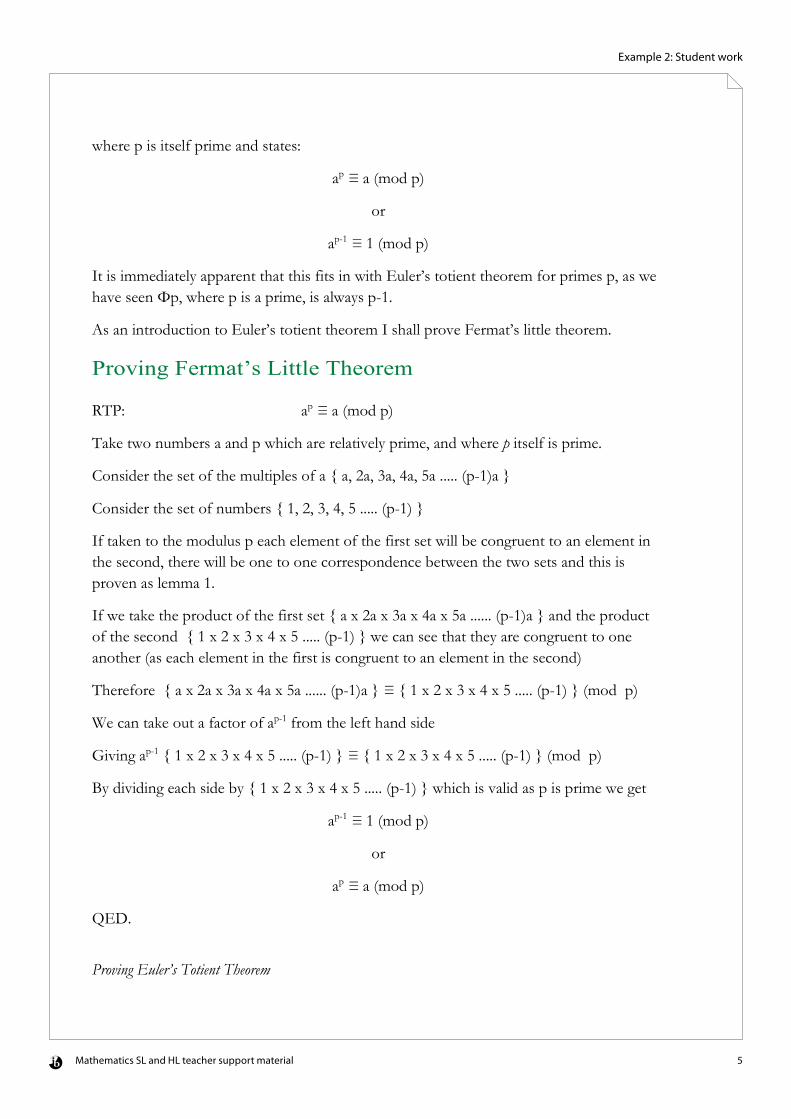
Proving Fermat’s Little Theorem RTP: ap ≡ a (mod p)
Take two numbers a and p which are relatively prime, and where p itself is prime.
Consider the set of the multiples of a { a, 2a, 3a, 4a, 5a ..... (p-1)a }
Consider the set of numbers { 1, 2, 3, 4, 5 ..... (p-1) }
If taken to the modulus p each element of the first set will be congruent to an element in the second, there will be one to one correspondence between the two sets and this is proven as lemma 1.
If we take the product of the first set { a x 2a x 3a x 4a x 5a ...... (p-1)a } and the product of the second { 1 x 2 x 3 x 4 x 5 ..... (p-1) } we can see that they are congruent to one another (as each element in the first is congruent to an element in the second)
Therefore { a x 2a x 3a x 4a x 5a ...... (p-1)a } ≡ { 1 x 2 x 3 x 4 x 5 ..... (p-1) } (mod p)
We can take out a factor of ap-1 from the left hand side
Giving ap-1 { 1 x 2 x 3 x 4 x 5 ..... (p-1) } ≡ { 1 x 2 x 3 x 4 x 5 ..... (p-1) } (mod p)
By dividing each side by { 1 x 2 x 3 x 4 x 5 ..... (p-1) } which is valid as p is prime we get
ap-1 ≡ 1 (mod p)
or
ap ≡ a (mod p)
QED.
Mathematics SL and HL teacher support material 6
Example 2: Student work
Proving Euler’s Totient Theorem
Lemma 1: Each number in the first set must be congruent to one and only one number in the second and each number in the second set must be congruent to one and only one number in the first. This may not be obvious at first but can be proved through three logical steps.
(1) Each number in the first set must be congruent to one of the elements in the second as all possible congruences save 0 are present, none will be congruent to 0 as a and p are relatively prime.
(2) A number cannot be congruent to two numbers in the second set as a number can only be congruent to numbers which differ by a multiple of p, as all elements of the second set are smaller than p a number can only be congruent to one of them.
(3) No two numbers in the first set, call them ba and ca, can be congruent to the same number in the second. This would indicate that the two numbers were congruent to each other ba ≡ ca (mod p) which would indicate that b ≡ c (mod p) which is not true as they are both different and less than p itself.
Therefore, through these three steps Lemma 1 is proven.
Proving Euler’s Totient Theorem As Fermat’s little theorem is a special case of Euler’s totient theorem (where n is prime) the two proofs are quite similar and in fact only slight adjustments need to be made to the proof of Fermat’s little theorem to give you Euler’s totient theorem4. RTP: aΦn ≡ 1 (mod n)
Take two numbers, a and n which are relatively prime
Consider the set N of numbers that are relatively prime to n { 1, n1, n2...nΦn }
This set will have Φn elements (Φn is defined as the number of numbers relatively prime to n)
Consider the set aN, where each element is the product of a and an element of N { a, an1, an2... anΦn }
Each element in set aN will be congruent to an element in set N (mod n), this is follows by the same argument as in lemma 1 and so the two sets will be congruent to each other
Therefore { a x an1 x an2 x ... x anΦn } ≡ { 1 x n1 x n2 x ... x nΦn } (mod n)
4 http://planetmath.org/?op=getobj&from=objects&id=335
Mathematics SL and HL teacher support material 7
Example 2: Student work
Proving Euler’s Totient Theorem
By taking out a factor of aΦn from the left hand side we get
aΦn { 1 x n1 x n2 x ... x nΦn } ≡ { 1 x n1 x n2 x ... x nΦn } (mod n)
If we then divide through by { 1 x n1 x n2 x ... x nΦn } which is valid as all elements are relatively prime to n we get
aΦn ≡ 1 (mod n)
QED.
Applications Unlike some of Euler’s other work in number theory such as his proof of the two square theorem Euler’s totient theorem has very real uses and applications in the world and like much of number theory those uses are almost exclusively in the world of cryptography and cryptanalysis. Both Fermat’s little theorem and Euler’s totient theorem are used in the encryption and decryption of data, specifically in the RSA encryption system5, whose protection revolves around large prime numbers raised to large powers being difficult to factorise.
Conclusion This theorem may not be Euler’s most elegant piece of mathematics (my personal favourite is his proof of the two square theorem by infinite descent) or at the time seemed like his most important piece of work at the time but this, in number theory at least, is probably his most useful piece of mathematics to the world today.
This proof has given me a chance to link up some of the work I have done in the largely separate discrete mathematics and sets relations and groups options. These two options appear to me to be the purest sections of mathematics that I have studied but are for whatever reason seldom linked in class, this project has allowed me to explore the links between them and use knowledge from one in relation to the other, broadening my view of maths.
5 http://www.muppetlabs.com/~breadbox/txt/rsa.html#7
A Complete. Achieves aim. Concise!
D Reflection. Linking mathematical ideas
A Conclusion
C Personally involved

Euler’s totient theorem. He then asked to do a pure mathematics exploration. He absolutely didunderstand everything he wrote. If only all students were like him!”
The teacher’s comment provides evidence that the student was personally engaged in theexploration and explains why some of the terms were not fully defined, as they were fullyunderstood by the student and his class, which was his intended audience.
Assessment
Criterion A B C D E (SL) E (HL) Total (SL) Total (HL)Achievement level awarded 3 3 2 2 6 6 16 16
Maximum possible achievement level 4 3 4 3 6 6 20 20
Comments
Criterion A: Communication
A3—The work is concise, as it proves the conjecture in fewer than seven pages. It fulfills theaims, is well organized and complete. The exploration would benefit from more completeexplanations (refer to page 7 annotation).
Criterion B: Mathematical presentation
B3—Condone use of “N” rather than “n” in the table on page 4. The class was familiar with themodular arithmetic, so definitions were not needed.
Criterion C: Personal engagement
C2—There was evidence of sufficient personal interest to award a level 2.
Criterion D: Reflection
D2—It links areas of maths. There is reflection on the elegance of the mathematics (page 7).
SL Criterion E: Use of mathematics
E6—It is highly unlikely that a mathematics SL student will produce work of this calibre, but itobviously achieves level 6.
HL Criterion E: Use of mathematics
E6—It is commensurate with the level of the course, precise and demonstrates thoroughknowledge, insight, sophistication and the rigour expected for mathematics HL.
General comments
Background information from the teacher:
“The student is a further mathematician and as such has been taught the ‘Discrete’ and ‘Sets,relations and groups’ options. He is therefore familiar with the language of modular arithmeticand had encountered Fermat’s little theorem in class. The proof of this theorem, although notrequired in the syllabus, was set as a homework. In his research of this, he also encountered

Euler’s totient theorem. He then asked to do a pure mathematics exploration. He absolutely didunderstand everything he wrote. If only all students were like him!”
The teacher’s comment provides evidence that the student was personally engaged in theexploration and explains why some of the terms were not fully defined, as they were fullyunderstood by the student and his class, which was his intended audience.

Mathematics SL and HL teacher support material 1
Example 6: Student work
The Polar Area Diagrams of Florence Nightingale If you read the article on Florence Nightingale in “The Children’s Book of Famous Lives”1 you will not learn that she had to battle with her parents to be allowed to study Mathematics. If you read the Ladybird book “Florence Nightingale”2 you will not discover that she was the first woman to be elected as a Fellow of the Royal Statistical Society. In looking around for an area of research I was intrigued to discover that Florence Nightingale, who I always thought of as the “lady with the lamp”, was a competent Mathematician who created her own type of statistical diagram which she used to save thousands of soldiers from needless death. Florence Nightingale headed a group of 38 nurses who went to clean up the hospitals for the British soldiers in the Crimea in 1854. She found that most of the deaths were due to diseases which could be prevented by basic hygiene, such as typhus and cholera. Her improvements were simple but they had an enormous effect:
“She and her nurses washed and bathed the soldiers, laundered their linens, gave them clean beds to lie in, and fed them”3.
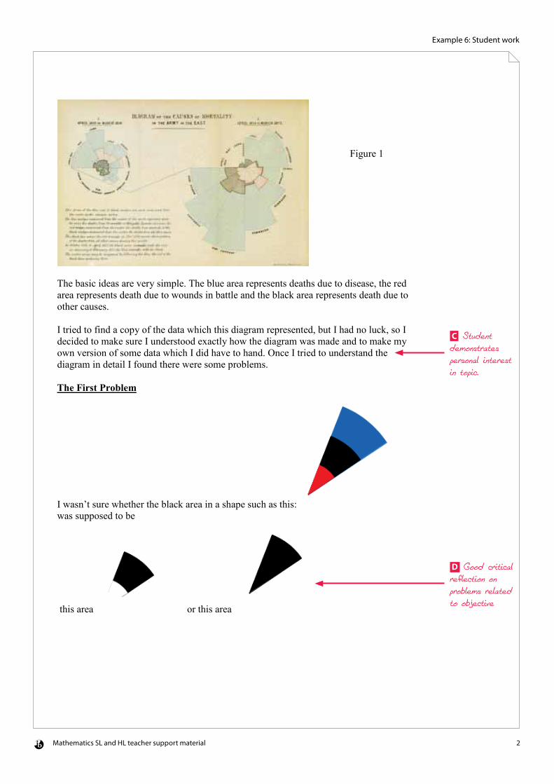
When she returned to Britain she made a detailed report to the Government setting out what conditions were like and what needed to be done to reduce deaths in the hospitals. Nothing was done, so she tried again, making another statistical report and included in it three new statistical diagrams to make data collated by William Farr more accessible to people who could not get their minds around tables of figures. These were her polar area diagrams or rose diagrams, sometimes also known as ‘coxcombs’. The first showed how many men had died over the two years 1854-5, the second showed what proportions of men had died from wounds in battle, from disease and from other causes, the third showed how the number of deaths had decreased once “sanitary improvements”4 had been introduced. I decided I would try to recreate the second of these diagrams which is the most complicated and the most shocking. It is called “Diagram of the causes of mortality in the army in the east”. A copy of it is below:
A Rationale and aim included in introduction
Mathematics SL and HL teacher support material 2
Example 6: Student work
The basic ideas are very simple. The blue area represents deaths due to disease, the red area represents death due to wounds in battle and the black area represents death due to other causes. I tried to find a copy of the data which this diagram represented, but I had no luck, so I decided to make sure I understood exactly how the diagram was made and to make my own version of some data which I did have to hand. Once I tried to understand the diagram in detail I found there were some problems. The First Problem
I wasn’t sure whether the black area in a shape such as this: was supposed to be
this area or this area
Figure 1
C Student demonstrates personal interest in topic.
D Good critical reflection on problems related to objective
Mathematics SL and HL teacher support material 3
Example 6: Student work
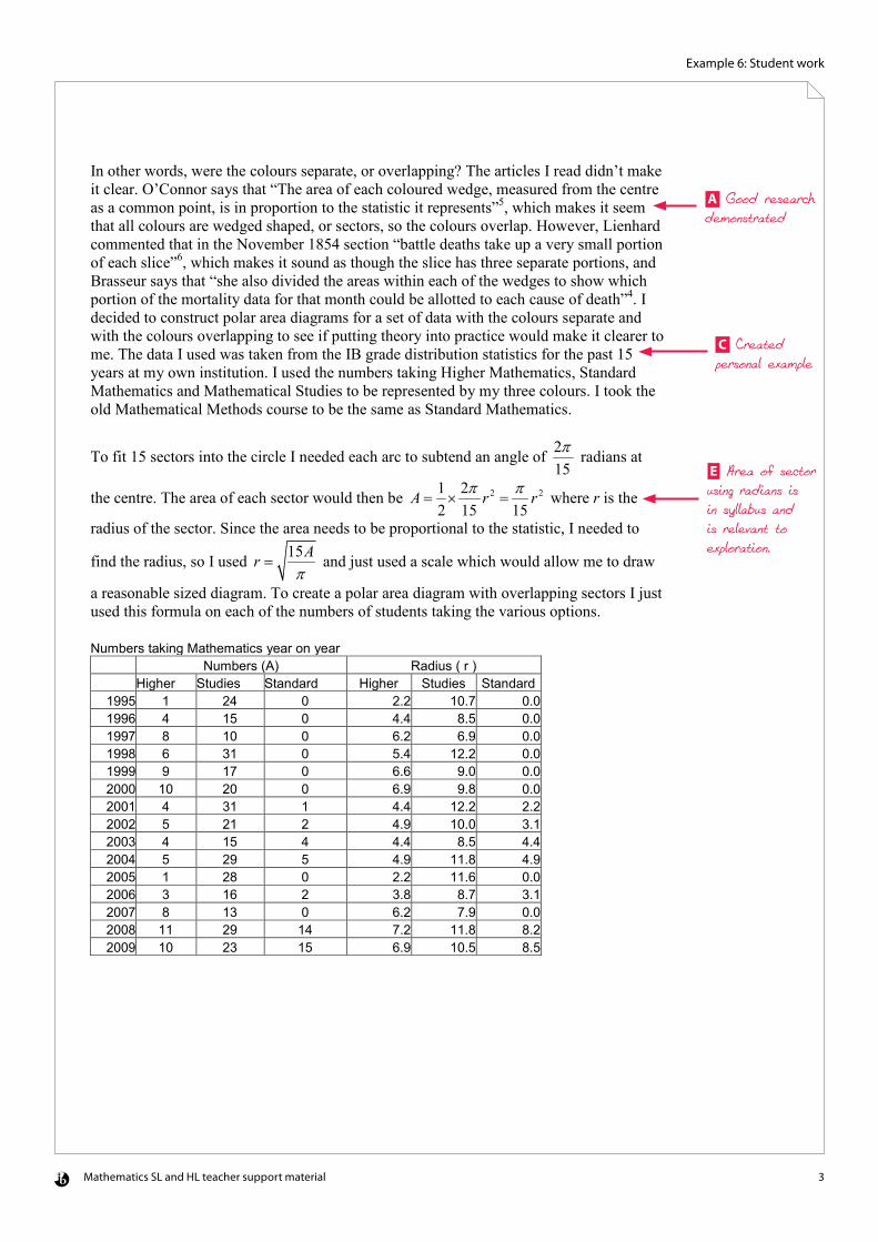
In other words, were the colours separate, or overlapping? The articles I read didn’t make it clear. O’Connor says that “The area of each coloured wedge, measured from the centre as a common point, is in proportion to the statistic it represents”5, which makes it seem that all colours are wedged shaped, or sectors, so the colours overlap. However, Lienhard commented that in the November 1854 section “battle deaths take up a very small portion of each slice”6, which makes it sound as though the slice has three separate portions, and Brasseur says that “she also divided the areas within each of the wedges to show which portion of the mortality data for that month could be allotted to each cause of death”4. I decided to construct polar area diagrams for a set of data with the colours separate and with the colours overlapping to see if putting theory into practice would make it clearer to me. The data I used was taken from the IB grade distribution statistics for the past 15 years at my own institution. I used the numbers taking Higher Mathematics, Standard Mathematics and Mathematical Studies to be represented by my three colours. I took the old Mathematical Methods course to be the same as Standard Mathematics.
To fit 15 sectors into the circle I needed each arc to subtend an angle of 215π radians at
the centre. The area of each sector would then be 2 21 22 15 15
A r rπ π= × = where r is the
radius of the sector. Since the area needs to be proportional to the statistic, I needed to
find the radius, so I used 15Arπ
= and just used a scale which would allow me to draw
a reasonable sized diagram. To create a polar area diagram with overlapping sectors I just used this formula on each of the numbers of students taking the various options. Numbers taking Mathematics year on year Numbers (A) Radius ( r ) Higher Studies Standard Higher Studies Standard
1995 1 24 0 2.2 10.7 0.0 1996 4 15 0 4.4 8.5 0.0 1997 8 10 0 6.2 6.9 0.0 1998 6 31 0 5.4 12.2 0.0 1999 9 17 0 6.6 9.0 0.0 2000 10 20 0 6.9 9.8 0.0 2001 4 31 1 4.4 12.2 2.2 2002 5 21 2 4.9 10.0 3.1 2003 4 15 4 4.4 8.5 4.4 2004 5 29 5 4.9 11.8 4.9 2005 1 28 0 2.2 11.6 0.0 2006 3 16 2 3.8 8.7 3.1 2007 8 13 0 6.2 7.9 0.0 2008 11 29 14 7.2 11.8 8.2 2009 10 23 15 6.9 10.5 8.5
A Good research demonstrated
C Created personal example
E Area of sector using radians is in syllabus and is relevant to exploration.
Mathematics SL and HL teacher support material 4
Example 6: Student work
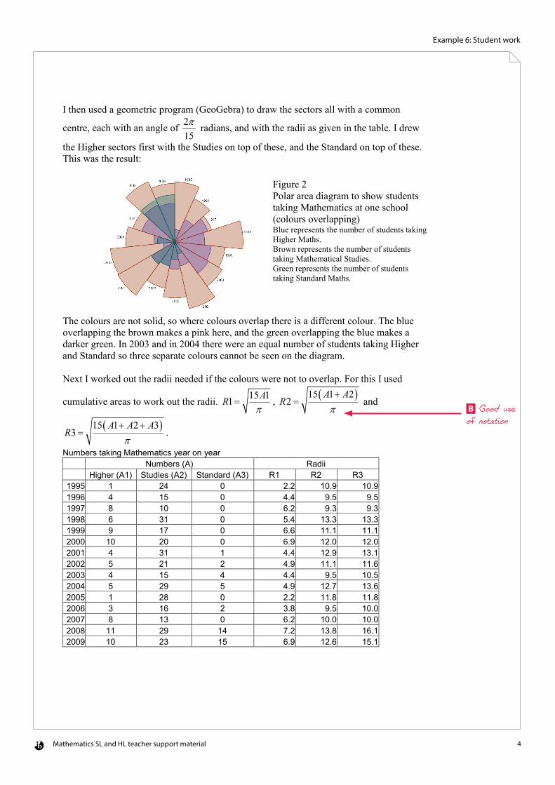
I then used a geometric program (GeoGebra) to draw the sectors all with a common
centre, each with an angle of 215π radians, and with the radii as given in the table. I drew
the Higher sectors first with the Studies on top of these, and the Standard on top of these. This was the result: The colours are not solid, so where colours overlap there is a different colour. The blue overlapping the brown makes a pink here, and the green overlapping the blue makes a darker green. In 2003 and in 2004 there were an equal number of students taking Higher and Standard so three separate colours cannot be seen on the diagram. Next I worked out the radii needed if the colours were not to overlap. For this I used
cumulative areas to work out the radii. 15 11 ARπ
= , ( )15 1 22
A AR
π+
= and
( )15 1 2 33
A A AR
π+ +
= .
Numbers taking Mathematics year on year Numbers (A) Radii Higher (A1) Studies (A2) Standard (A3) R1 R2 R3 1995 1 24 0 2.2 10.9 10.9 1996 4 15 0 4.4 9.5 9.5 1997 8 10 0 6.2 9.3 9.3 1998 6 31 0 5.4 13.3 13.3 1999 9 17 0 6.6 11.1 11.1 2000 10 20 0 6.9 12.0 12.0 2001 4 31 1 4.4 12.9 13.1 2002 5 21 2 4.9 11.1 11.6 2003 4 15 4 4.4 9.5 10.5 2004 5 29 5 4.9 12.7 13.6 2005 1 28 0 2.2 11.8 11.8 2006 3 16 2 3.8 9.5 10.0 2007 8 13 0 6.2 10.0 10.0 2008 11 29 14 7.2 13.8 16.1 2009 10 23 15 6.9 12.6 15.1
Figure 2 Polar area diagram to show students taking Mathematics at one school (colours overlapping) Blue represents the number of students taking Higher Maths. Brown represents the number of students taking Mathematical Studies. Green represents the number of students taking Standard Maths.
B Good use of notation
Mathematics SL and HL teacher support material 5
Example 6: Student work
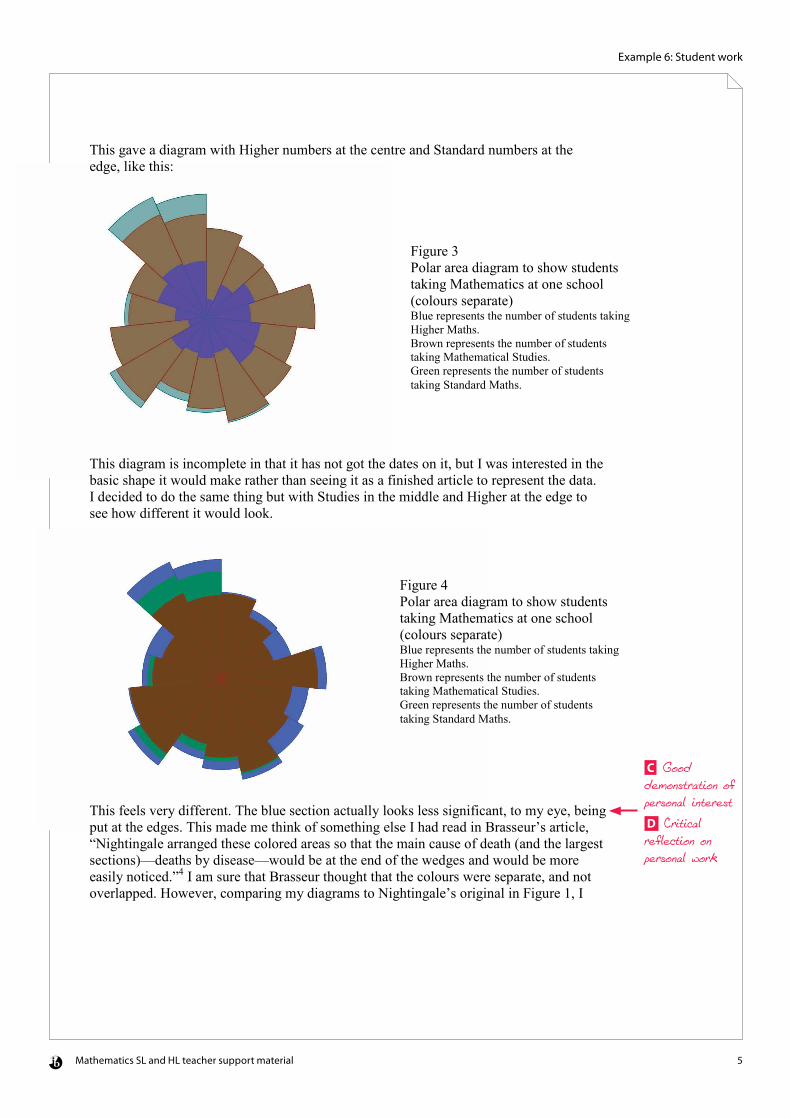
This gave a diagram with Higher numbers at the centre and Standard numbers at the edge, like this: This diagram is incomplete in that it has not got the dates on it, but I was interested in the basic shape it would make rather than seeing it as a finished article to represent the data. I decided to do the same thing but with Studies in the middle and Higher at the edge to see how different it would look. This feels very different. The blue section actually looks less significant, to my eye, being put at the edges. This made me think of something else I had read in Brasseur’s article, “Nightingale arranged these colored areas so that the main cause of death (and the largest sections)—deaths by disease—would be at the end of the wedges and would be more easily noticed.”4 I am sure that Brasseur thought that the colours were separate, and not overlapped. However, comparing my diagrams to Nightingale’s original in Figure 1, I
Figure 3 Polar area diagram to show students taking Mathematics at one school (colours separate) Blue represents the number of students taking Higher Maths. Brown represents the number of students taking Mathematical Studies. Green represents the number of students taking Standard Maths.
Figure 4 Polar area diagram to show students taking Mathematics at one school (colours separate) Blue represents the number of students taking Higher Maths. Brown represents the number of students taking Mathematical Studies. Green represents the number of students taking Standard Maths.
C Good demonstration of personal interest
D Critical reflection on personal work
Mathematics SL and HL teacher support material 6
Example 6: Student work
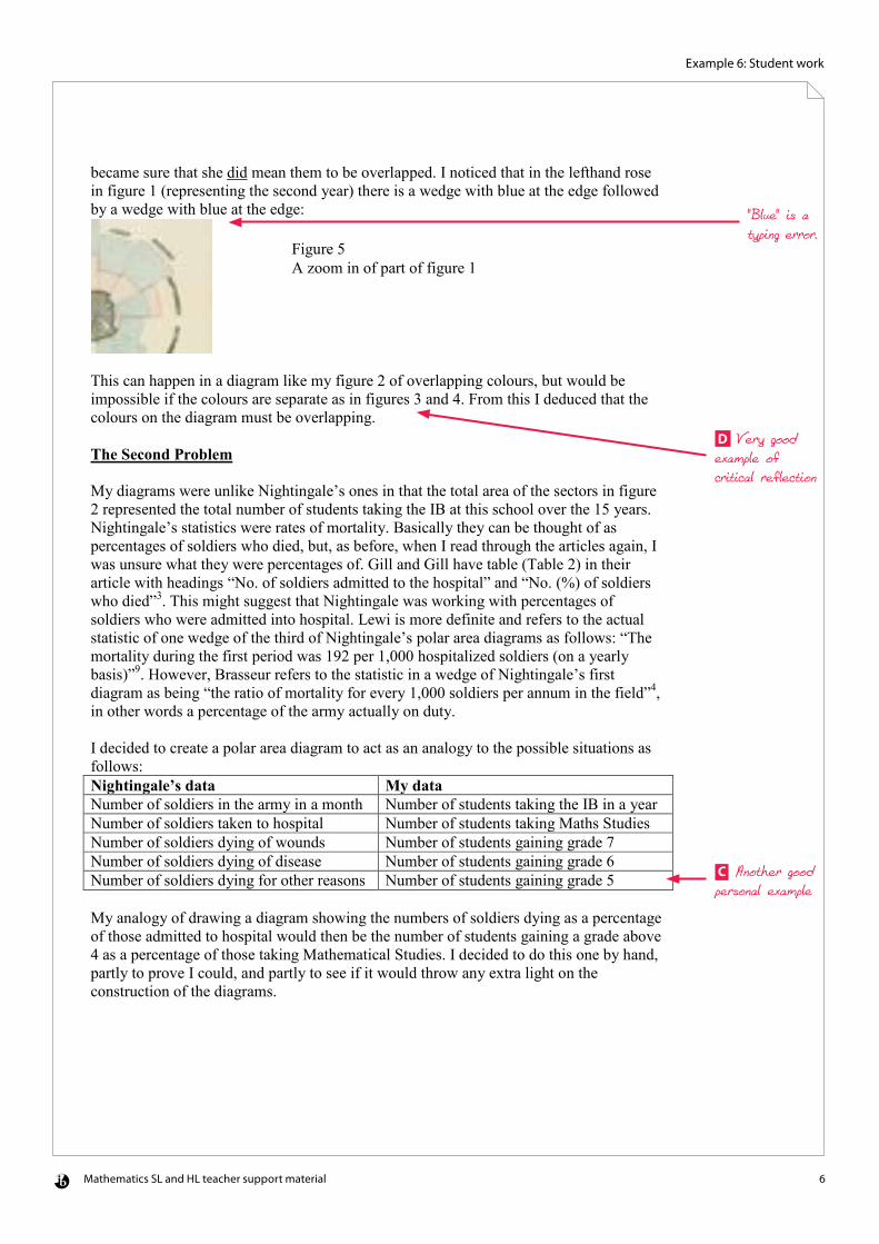
became sure that she did mean them to be overlapped. I noticed that in the lefthand rose in figure 1 (representing the second year) there is a wedge with blue at the edge followed by a wedge with blue at the edge:
This can happen in a diagram like my figure 2 of overlapping colours, but would be impossible if the colours are separate as in figures 3 and 4. From this I deduced that the colours on the diagram must be overlapping. The Second Problem My diagrams were unlike Nightingale’s ones in that the total area of the sectors in figure 2 represented the total number of students taking the IB at this school over the 15 years. Nightingale’s statistics were rates of mortality. Basically they can be thought of as percentages of soldiers who died, but, as before, when I read through the articles again, I was unsure what they were percentages of. Gill and Gill have table (Table 2) in their article with headings “No. of soldiers admitted to the hospital” and “No. (%) of soldiers who died”3. This might suggest that Nightingale was working with percentages of soldiers who were admitted into hospital. Lewi is more definite and refers to the actual statistic of one wedge of the third of Nightingale’s polar area diagrams as follows: “The mortality during the first period was 192 per 1,000 hospitalized soldiers (on a yearly basis)”9. However, Brasseur refers to the statistic in a wedge of Nightingale’s first diagram as being “the ratio of mortality for every 1,000 soldiers per annum in the field”4, in other words a percentage of the army actually on duty. I decided to create a polar area diagram to act as an analogy to the possible situations as follows: Nightingale’s data My data Number of soldiers in the army in a month Number of students taking the IB in a year Number of soldiers taken to hospital Number of students taking Maths Studies Number of soldiers dying of wounds Number of students gaining grade 7 Number of soldiers dying of disease Number of students gaining grade 6 Number of soldiers dying for other reasons Number of students gaining grade 5 My analogy of drawing a diagram showing the numbers of soldiers dying as a percentage of those admitted to hospital would then be the number of students gaining a grade above 4 as a percentage of those taking Mathematical Studies. I decided to do this one by hand, partly to prove I could, and partly to see if it would throw any extra light on the construction of the diagrams.
Figure 5 A zoom in of part of figure 1
"Blue" is a typing error.
D Very good example of critical reflection
C Another good personal example
Mathematics SL and HL teacher support material 7
Example 6: Student work
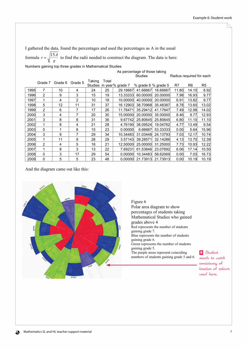
I gathered the data, found the percentages and used the percentages as A in the usual
formula 15Arπ
= to find the radii needed to construct the diagram. The data is here:
Numbers gaining top three grades in Mathematical Studies
As percentage of those taking
Studies Radius required for each
Grade 7 Grade 6 Grade 5 Taking
Studies Total
in year % grade 7 % grade 6 % grade 5 R7 R6 R5 1995 7 10 4 24 25 29.16667 41.66667 16.66667 11.80 14.10 8.92 1996 2 9 3 15 19 13.33333 60.00000 20.00000 7.98 16.93 9.77 1997 1 4 2 10 18 10.00000 40.00000 20.00000 6.91 13.82 9.77 1998 5 12 11 31 37 16.12903 38.70968 35.48387 8.78 13.60 13.02 1999 2 6 7 17 26 11.76471 35.29412 41.17647 7.49 12.98 14.02 2000 3 4 7 20 30 15.00000 20.00000 35.00000 8.46 9.77 12.93 2001 3 8 8 31 36 9.67742 25.80645 25.80645 6.80 11.10 11.10 2002 1 8 4 21 28 4.76190 38.09524 19.04762 4.77 13.49 9.54 2003 0 1 8 15 23 0.00000 6.66667 53.33333 0.00 5.64 15.96 2004 3 9 7 29 34 10.34483 31.03448 24.13793 7.03 12.17 10.74 2005 1 11 9 28 29 3.57143 39.28571 32.14286 4.13 13.70 12.39 2006 2 4 5 16 21 12.50000 25.00000 31.25000 7.73 10.93 12.22 2007 1 8 3 13 22 7.69231 61.53846 23.07692 6.06 17.14 10.50 2008 0 3 17 29 54 0.00000 10.34483 58.62069 0.00 7.03 16.73 2009 0 5 5 23 48 0.00000 21.73913 21.73913 0.00 10.19 10.19
And the diagram came out like this:
Figure 6 Polar area diagram to show percentages of students taking Mathematical Studies who gained grades above 4 Red represents the number of students gaining grade 7. Blue represents the number of students gaining grade 6. Green represents the number of students gaining grade 5. The purple areas represent coinciding numbers of students gaining grade 5 and 6.
B Student needs to watch consistency of location of colours used here.
Mathematics SL and HL teacher support material 8
Example 6: Student work
One thing which I learnt from this exercise is that you have to be very careful about your scale and think through every move before you start if you don’t want to fall off the edge of the paper! It is a far more tense experience drawing a diagram by hand because you know that one slip will make the whole diagram flawed. A computer slip can be corrected before you print out the result. My admiration for Florence Nightingale’s draftsmanship was heightened by doing this. The other thing which drawing by hand brought out was that, if you draw the arcs in in the appropriate colours, the colouring of the sectors sorts itself out. You colour from the arc inwards until you come to another arc or the centre. The only problem came when two arcs of different colours came in exactly the same place. I got around this problem by colouring these areas in a totally different colour and saying so at the side. At this point in my research someone suggested some more possible websites to me, and following these up I found a copy of Nightingale’s second diagram which was clear enough for me to read her notes, and a copy of the original data she used. The first of these was in a letter by Henry Woodbury suggesting that Nightingale got her calculations wrong and the radii represented the statistics rather than the area.7 The letter had a comment posted by Ian Short which led me to an article by him8 giving the data for the second diagram and explaining how it was created. The very clear reproduction of Nightingale’s second diagram in Woodbury’s letter7 shows that Miss Nightingale wrote beside it: “The areas of the blue, red and black wedges are each measured from the centre as the common vertex”. This makes it quite clear that the colours are overlapped and so solves my first problem. She also wrote “In October 1854 & April 1855 the black area coincides with the red”. She coloured the first of these in red and the second in black, but just commented on it beside the diagram to make it clear. The article by Short8 was a joy to read, although I could only work out the mathematical equations, which were written out in a way which is strange to me ( for example “$$ \text{Area of sector B} = \frac{\pi r_B^2}{3}=3$$”8 ) because I already knew what they were (The example had a sector B in a diagram which I could see had
2 21 22 3 3B BareaB r rπ π
= = ). The two things I found exciting from this article were the
table of data which Nightingale used to create the second diagram, and an explanation of what rates of mortality she used. She described these as follows; “The ratios of deaths and admissions to Force per 1000 per annum are calculated from the monthly ratios given in Dr. Smith’s Table B”4 and I had not been able to understand the meaning of this from the other articles. (Brasseur adds that “Dr. Smith was the late director-general of the army.”4). Using Short’s article I was able to work out what it meant. I will use an example of data taken from the table in Short’s article, which is in turn taken from “A contribution to the sanitary history of the British army during the late war with Russia” by Florence Nightingale of 18598. In February 1855 the average size of the army was 30919. Of these 2120 died of ‘zymotic diseases’, 42 died of ‘wounds & injuries’ and 361 died of ‘all other causes’. This gives a total of 2120 42 361 2523+ + = deaths. 2523
C This section shows a lot of personal interest.
Mathematics SL and HL teacher support material 9
Example 6: Student work
out of 30919 means that 2523 1000 81.600330919
× = men died per 1000 men in the army in
that month. If the size of the army had stayed at 30919, with no more men being shipped in or out, and the death rate had continued at 81.6 deaths per 1000 men per month over 12 months, the number of deaths per annum would have been 81.6003 12 979.2× = per 1000 men in the army. In other words 979.2 deaths per 1000 per annum. This understanding of the units used allowed me to finally understand why O’Connor says of the death rate in January 1855, “if this rate had continued, and troops had not been replaced frequently, then disease alone would have killed the entire British army in the Crimea.”5 The number of deaths due to disease in January 1855 was 2761 and the
average size of the army was 32393. This gives a rate of 2761 1000 12 1022.832393
× × =
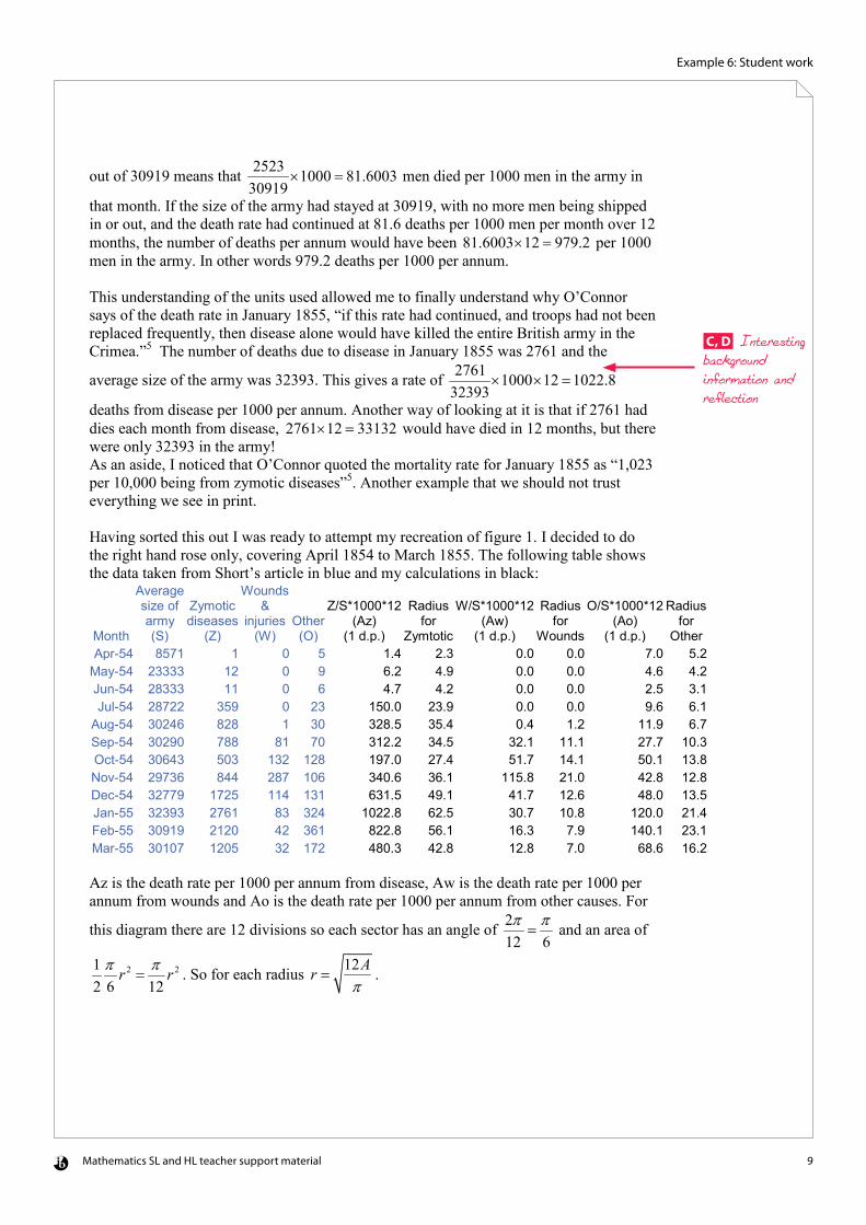
deaths from disease per 1000 per annum. Another way of looking at it is that if 2761 had dies each month from disease, 2761 12 33132× = would have died in 12 months, but there were only 32393 in the army! As an aside, I noticed that O’Connor quoted the mortality rate for January 1855 as “1,023 per 10,000 being from zymotic diseases”5. Another example that we should not trust everything we see in print. Having sorted this out I was ready to attempt my recreation of figure 1. I decided to do the right hand rose only, covering April 1854 to March 1855. The following table shows the data taken from Short’s article in blue and my calculations in black:
Month
Average size of army (S)
Zymotic diseases
(Z)
Wounds &
injuries (W)
Other (O)
Z/S*1000*12 (Az)
(1 d.p.)
Radius for
Zymtotic
W/S*1000*12 (Aw)
(1 d.p.)
Radius for
Wounds
O/S*1000*12 (Ao)
(1 d.p.)
Radius for
Other Apr-54 8571 1 0 5 1.4 2.3 0.0 0.0 7.0 5.2
May-54 23333 12 0 9 6.2 4.9 0.0 0.0 4.6 4.2 Jun-54 28333 11 0 6 4.7 4.2 0.0 0.0 2.5 3.1 Jul-54 28722 359 0 23 150.0 23.9 0.0 0.0 9.6 6.1
Aug-54 30246 828 1 30 328.5 35.4 0.4 1.2 11.9 6.7 Sep-54 30290 788 81 70 312.2 34.5 32.1 11.1 27.7 10.3 Oct-54 30643 503 132 128 197.0 27.4 51.7 14.1 50.1 13.8 Nov-54 29736 844 287 106 340.6 36.1 115.8 21.0 42.8 12.8 Dec-54 32779 1725 114 131 631.5 49.1 41.7 12.6 48.0 13.5 Jan-55 32393 2761 83 324 1022.8 62.5 30.7 10.8 120.0 21.4 Feb-55 30919 2120 42 361 822.8 56.1 16.3 7.9 140.1 23.1 Mar-55 30107 1205 32 172 480.3 42.8 12.8 7.0 68.6 16.2 Az is the death rate per 1000 per annum from disease, Aw is the death rate per 1000 per annum from wounds and Ao is the death rate per 1000 per annum from other causes. For
this diagram there are 12 divisions so each sector has an angle of 212 6π π= and an area of
2 212 6 12
r rπ π= . So for each radius 12Ar
π= .
C, D Interesting background information and reflection
Mathematics SL and HL teacher support material 10
Example 6: Student work
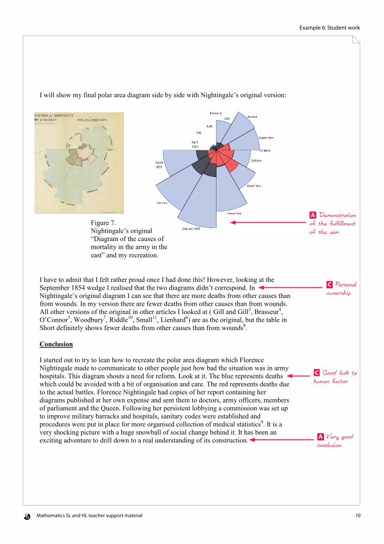
I will show my final polar area diagram side by side with Nightingale’s original version: I have to admit that I felt rather proud once I had done this! However, looking at the September 1854 wedge I realised that the two diagrams didn’t correspond. In Nightingale’s original diagram I can see that there are more deaths from other causes than from wounds. In my version there are fewer deaths from other causes than from wounds. All other versions of the original in other articles I looked at ( Gill and Gill3, Brasseur4, O’Connor5, Woodbury7, Riddle10, Small11, Lienhard6) are as the original, but the table in Short definitely shows fewer deaths from other causes than from wounds8. Conclusion I started out to try to lean how to recreate the polar area diagram which Florence Nightingale made to communicate to other people just how bad the situation was in army hospitals. This diagram shouts a need for reform. Look at it. The blue represents deaths which could be avoided with a bit of organisation and care. The red represents deaths due to the actual battles. Florence Nightingale had copies of her report containing her diagrams published at her own expense and sent them to doctors, army officers, members of parliament and the Queen. Following her persistent lobbying a commission was set up to improve military barracks and hospitals, sanitary codes were established and procedures were put in place for more organised collection of medical statistics4. It is a very shocking picture with a huge snowball of social change behind it. It has been an exciting adventure to drill down to a real understanding of its construction.
Figure 7. Nightingale’s original “Diagram of the causes of mortality in the army in the east” and my recreation.
A Demonstration of the fulfillment of the aim
C Personal ownership
C Good link to human factor
A Very good conclusion

Mathematics SL and HL teacher support material 11
Example 6: Student work
However, the biggest lesson I have learnt from this research is that you can’t trust what you read. As I have argued in the main text, I am moderately sure that Brasseur thought the colours of the second diagram did not overlap4, I think O’Connor got his death rates wrong for January 18555, and I think Short may have transcribed the data incorrectly for September 18548. According to Brasseur, Florence Nightingale cross checked her data and was systematic about addressing objections to her analysis4. Everyone can make mistakes, and errors can propagate if we just quote what someone else says without looking for corroboration. I have been left with a desire to find out more about this tenacious woman who wouldn’t let society mould her into a genteel wife. Also, if I ever get the chance, I would like to get a look at one of the 2000 copies of “Notes on Matters Affecting the Health, Effiency and Hospital Administration of the British Army. Founded Chiefly on the Experience of the Late War” which Florence Nightingale had published in 1858, to see the actual table of data and check the numbers for September 1854.
D Reflection on what has been learned
Mathematics SL and HL teacher support material 12
Example 6: Student work
References/Bibliography 1.Duthie, Eric ed. The Children’s Book of Famous Lives.Odhams Press Ltd, London 1957 2. Du Garde Peach, L. Florence Nightingale. Wills & Hepworth Ltd, Loughborough, 1959 3. Gill, Christopher J. and Gill, Gillian C. Nightingale in Scutari: Her Legacy Reexamined Center for Internatinal Health, Boston University School of Public Health, Boston, Massachusetts, <http://www.countryjoe.com/nightingale/FN%20in%20CID%20final.pdf > viewed 26th July 2009 4. Brasseur, Lee, Florence Nightingale’s Visual Rhetoric in the Rose Diagrams. Technical Communication Quarterly, 14(2), 161-182, Lawrence Erlbaum Associates, Inc, 2005, <http://benninghoff.emich.edu/424W06/handouts/Brasseur_Florence_Nightengale.pdf> viewed 26th July 2009 5. O’Connor, J.J. and Robertson, E.F., Florence Nightingale. <http://www-groups.dcs.st-and.ac.uk/~history/Biographies/Nightingale.html> viewed 26th July 2009 6. Lienhard, John H., Nightingale’s Graph, The Engines of Our Ingenuity. 2002 <http://www.uh.edu/engines/epi1712.htm> viewed 26th July 2009 7. Woodbury, Henry, Nightingale’s Rose. American Physical SocietyLaunches Dynamic Diagrams Redesign of Physical Review Letters, January 9, 2008, 4:05 pm, filed under Information Design, Visual Explanation <http://dd.dynamicdiagrams.com/2008/01/nightingales-rose/> Viewed 30th July 2009 8. Short, Ian, Mathematics of the Coxcombs. November 5th, 2008 <http://understandinguncertainty.org/node/214> viewed 30th July 2009 9. Lewi, Paul J. Florence Nightingale and Polar Area Diagrams, Speaking of Graphics. 2006 < www.datascope.be/sog/SOG-Chapter5.pdf> viewed 26th July 2009
10. Riddle, Larry, Polar-Area Diagram. 2006 , <http://www.scottlan.edu/lriddle/women/nightpiechart.htm> viewed 26th July 2009
11. Small, Hugh, Florence Nightingale’s statistical diagrams. Presentation to Research Conference organized by the Florence Nightingale Museum St. Thomas’s Hospital, 18th March 1998 <http://www.florence-nightingale-avenging-angel.co.uk/GraphicsPaper/Graphics.htm> viewed 26th July 2009
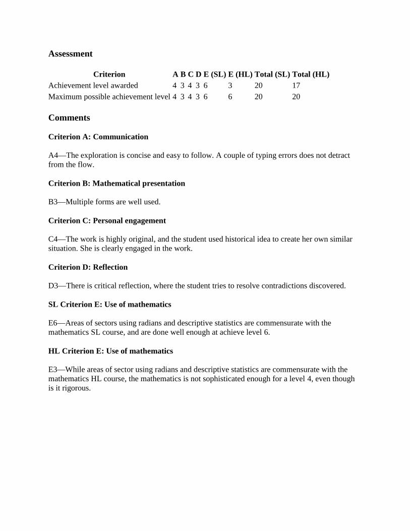
Assessment
Criterion A B C D E (SL) E (HL) Total (SL) Total (HL)Achievement level awarded 4 3 4 3 6 3 20 17
Maximum possible achievement level 4 3 4 3 6 6 20 20
Comments
Criterion A: Communication
A4—The exploration is concise and easy to follow. A couple of typing errors does not detractfrom the flow.
Criterion B: Mathematical presentation
B3—Multiple forms are well used.
Criterion C: Personal engagement
C4—The work is highly original, and the student used historical idea to create her own similarsituation. She is clearly engaged in the work.
Criterion D: Reflection
D3—There is critical reflection, where the student tries to resolve contradictions discovered.
SL Criterion E: Use of mathematics
E6—Areas of sectors using radians and descriptive statistics are commensurate with themathematics SL course, and are done well enough at achieve level 6.
HL Criterion E: Use of mathematics
E3—While areas of sector using radians and descriptive statistics are commensurate with themathematics HL course, the mathematics is not sophisticated enough for a level 4, even thoughis it rigorous.
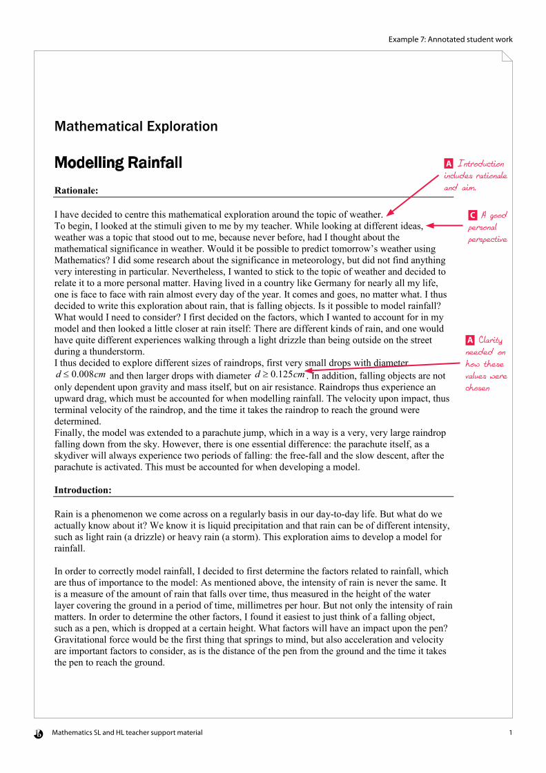
Mathematics SL and HL teacher support material 1
Example 7: Annotated student work
Mathematical Exploration Modelling Rainfall Rationale: I have decided to centre this mathematical exploration around the topic of weather. To begin, I looked at the stimuli given to me by my teacher. While looking at different ideas, weather was a topic that stood out to me, because never before, had I thought about the mathematical significance in weather. Would it be possible to predict tomorrow’s weather using Mathematics? I did some research about the significance in meteorology, but did not find anything very interesting in particular. Nevertheless, I wanted to stick to the topic of weather and decided to relate it to a more personal matter. Having lived in a country like Germany for nearly all my life, one is face to face with rain almost every day of the year. It comes and goes, no matter what. I thus decided to write this exploration about rain, that is falling objects. Is it possible to model rainfall? What would I need to consider? I first decided on the factors, which I wanted to account for in my model and then looked a little closer at rain itself: There are different kinds of rain, and one would have quite different experiences walking through a light drizzle than being outside on the street during a thunderstorm. I thus decided to explore different sizes of raindrops, first very small drops with diameter d ≤ 0.008cm and then larger drops with diameter d ≥ 0.125cm . In addition, falling objects are not only dependent upon gravity and mass itself, but on air resistance. Raindrops thus experience an upward drag, which must be accounted for when modelling rainfall. The velocity upon impact, thus terminal velocity of the raindrop, and the time it takes the raindrop to reach the ground were determined. Finally, the model was extended to a parachute jump, which in a way is a very, very large raindrop falling down from the sky. However, there is one essential difference: the parachute itself, as a skydiver will always experience two periods of falling: the free-fall and the slow descent, after the parachute is activated. This must be accounted for when developing a model. Introduction: Rain is a phenomenon we come across on a regularly basis in our day-to-day life. But what do we actually know about it? We know it is liquid precipitation and that rain can be of different intensity, such as light rain (a drizzle) or heavy rain (a storm). This exploration aims to develop a model for rainfall. In order to correctly model rainfall, I decided to first determine the factors related to rainfall, which are thus of importance to the model: As mentioned above, the intensity of rain is never the same. It is a measure of the amount of rain that falls over time, thus measured in the height of the water layer covering the ground in a period of time, millimetres per hour. But not only the intensity of rain matters. In order to determine the other factors, I found it easiest to just think of a falling object, such as a pen, which is dropped at a certain height. What factors will have an impact upon the pen? Gravitational force would be the first thing that springs to mind, but also acceleration and velocity are important factors to consider, as is the distance of the pen from the ground and the time it takes the pen to reach the ground.
A Introduction includes rationale and aim.
C A good personal perspective
A Clarity needed on how these values were chosen
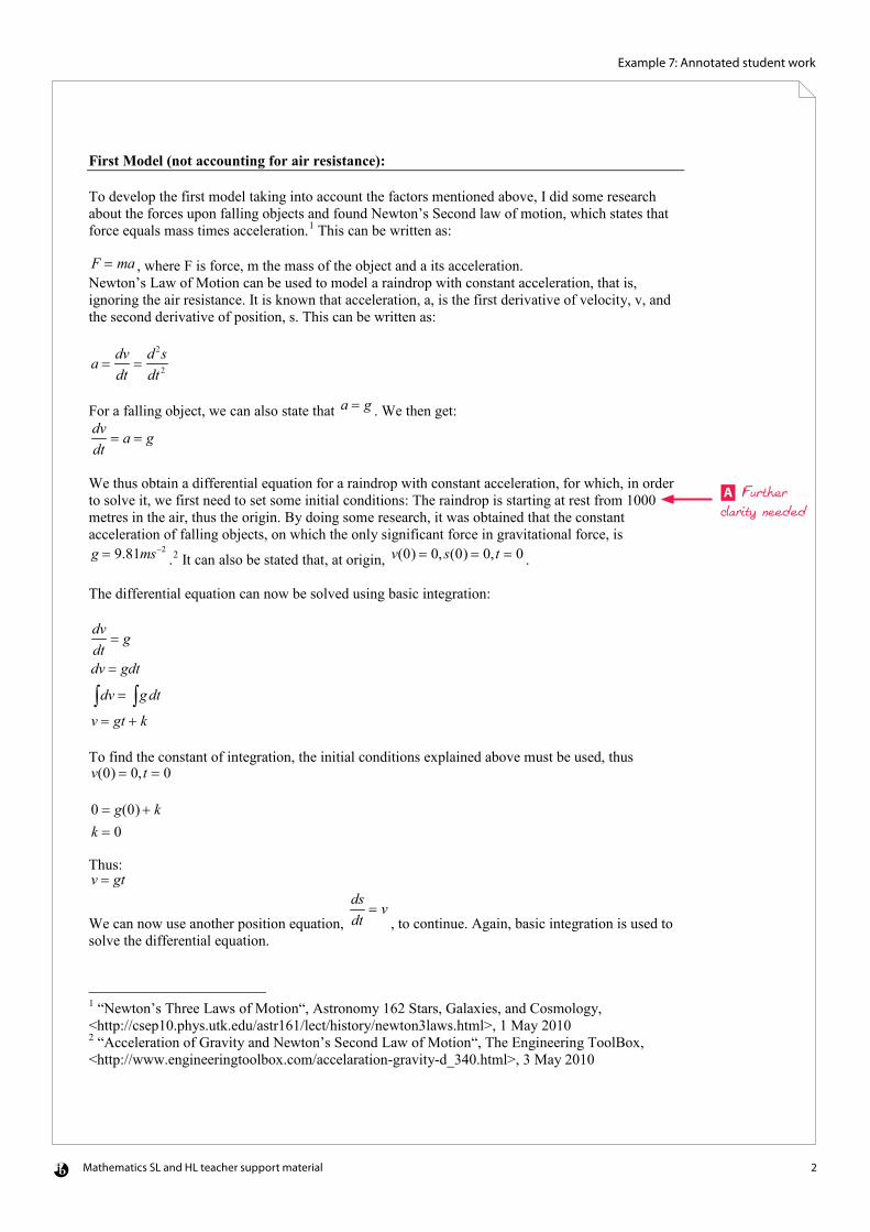
Mathematics SL and HL teacher support material 2
Example 7: Annotated student work
First Model (not accounting for air resistance): To develop the first model taking into account the factors mentioned above, I did some research about the forces upon falling objects and found Newton’s Second law of motion, which states that force equals mass times acceleration.1 This can be written as: F = ma , where F is force, m the mass of the object and a its acceleration. Newton’s Law of Motion can be used to model a raindrop with constant acceleration, that is, ignoring the air resistance. It is known that acceleration, a, is the first derivative of velocity, v, and the second derivative of position, s. This can be written as:
a =dvdt
=d 2sdt 2
For a falling object, we can also state that a = g . We then get: dvdt
= a = g
We thus obtain a differential equation for a raindrop with constant acceleration, for which, in order to solve it, we first need to set some initial conditions: The raindrop is starting at rest from 1000 metres in the air, thus the origin. By doing some research, it was obtained that the constant acceleration of falling objects, on which the only significant force in gravitational force, is g = 9.81ms−2
.2 It can also be stated that, at origin, v(0) = 0, s(0) = 0,t = 0 . The differential equation can now be solved using basic integration: dvdt
= g
dv = gdt
dv∫ = gdt∫v = gt + k To find the constant of integration, the initial conditions explained above must be used, thus v(0) = 0,t = 0 0 = g(0) + kk = 0 Thus: v = gt
We can now use another position equation,
dsdt
= v, to continue. Again, basic integration is used to
solve the differential equation.
1 “Newton’s Three Laws of Motion“, Astronomy 162 Stars, Galaxies, and Cosmology, <http://csep10.phys.utk.edu/astr161/lect/history/newton3laws.html>, 1 May 2010 2 “Acceleration of Gravity and Newton’s Second Law of Motion“, The Engineering ToolBox, <http://www.engineeringtoolbox.com/accelaration-gravity-d_340.html>, 3 May 2010
A Further clarity needed
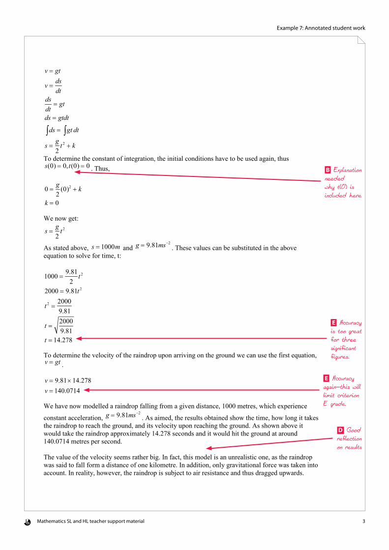
Mathematics SL and HL teacher support material 3
Example 7: Annotated student work
v = gt
v = dsdt
dsdt
= gt
ds = gtdt
ds∫ = gt dt∫ s = g
2t 2 + k
To determine the constant of integration, the initial conditions have to be used again, thus s(0) = 0,t(0) = 0 . Thus,
0 =g2
(0)2 + k
k = 0 We now get:
s = g2
t 2
As stated above, s = 1000m and g = 9.81ms−2
. These values can be substituted in the above equation to solve for time, t:
1000 =9.81
2t 2
2000 = 9.81t 2
t 2 =20009.81
t = 20009.81
t = 14.278 To determine the velocity of the raindrop upon arriving on the ground we can use the first equation, v = gt . v = 9.81×14.278v = 140.0714 We have now modelled a raindrop falling from a given distance, 1000 metres, which experience
constant acceleration, g = 9.81ms−2. As aimed, the results obtained show the time, how long it takes
the raindrop to reach the ground, and its velocity upon reaching the ground. As shown above it would take the raindrop approximately 14.278 seconds and it would hit the ground at around 140.0714 metres per second. The value of the velocity seems rather big. In fact, this model is an unrealistic one, as the raindrop was said to fall form a distance of one kilometre. In addition, only gravitational force was taken into account. In reality, however, the raindrop is subject to air resistance and thus dragged upwards.
B Explanation needed why t(0) is included here
E Accuracy is too great for three significant figures.
E Accuracy again—this will limit criterion E grade.
D Good reflection on results
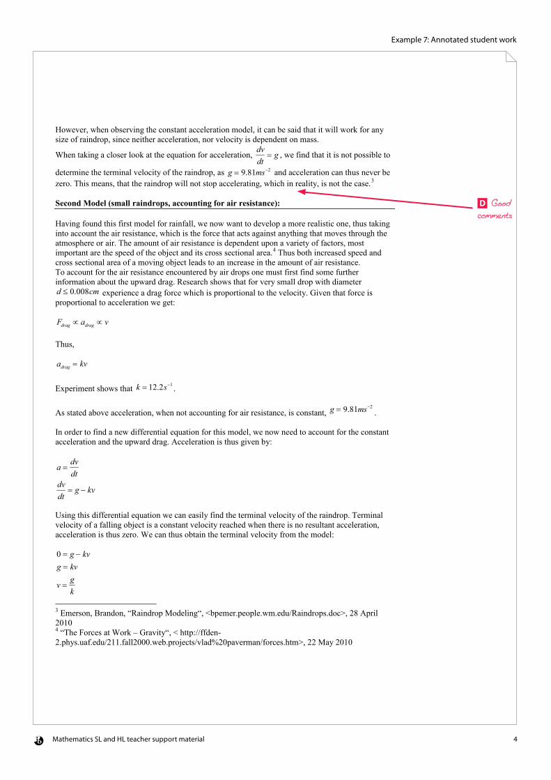
Mathematics SL and HL teacher support material 4
Example 7: Annotated student work
However, when observing the constant acceleration model, it can be said that it will work for any size of raindrop, since neither acceleration, nor velocity is dependent on mass.
When taking a closer look at the equation for acceleration, dvdt
= g , we find that it is not possible to
determine the terminal velocity of the raindrop, as g = 9.81ms−2 and acceleration can thus never be zero. This means, that the raindrop will not stop accelerating, which in reality, is not the case.3 Second Model (small raindrops, accounting for air resistance): Having found this first model for rainfall, we now want to develop a more realistic one, thus taking into account the air resistance, which is the force that acts against anything that moves through the atmosphere or air. The amount of air resistance is dependent upon a variety of factors, most important are the speed of the object and its cross sectional area.4 Thus both increased speed and cross sectional area of a moving object leads to an increase in the amount of air resistance. To account for the air resistance encountered by air drops one must first find some further information about the upward drag. Research shows that for very small drop with diameter d ≤ 0.008cm experience a drag force which is proportional to the velocity. Given that force is proportional to acceleration we get: Fdrag ∝ adrag ∝ v Thus, adrag = kv Experiment shows that k = 12.2s−1 .
As stated above acceleration, when not accounting for air resistance, is constant, g = 9.81ms−2.
In order to find a new differential equation for this model, we now need to account for the constant acceleration and the upward drag. Acceleration is thus given by:
a =dvdt
dvdt
= g − kv
Using this differential equation we can easily find the terminal velocity of the raindrop. Terminal velocity of a falling object is a constant velocity reached when there is no resultant acceleration, acceleration is thus zero. We can thus obtain the terminal velocity from the model: 0 = g − kvg = kv
v = gk
3 Emerson, Brandon, “Raindrop Modeling“, <bpemer.people.wm.edu/Raindrops.doc>, 28 April 2010 4 “The Forces at Work – Gravity“, < http://ffden-2.phys.uaf.edu/211.fall2000.web.projects/vlad%20paverman/forces.htm>, 22 May 2010
D Good comments
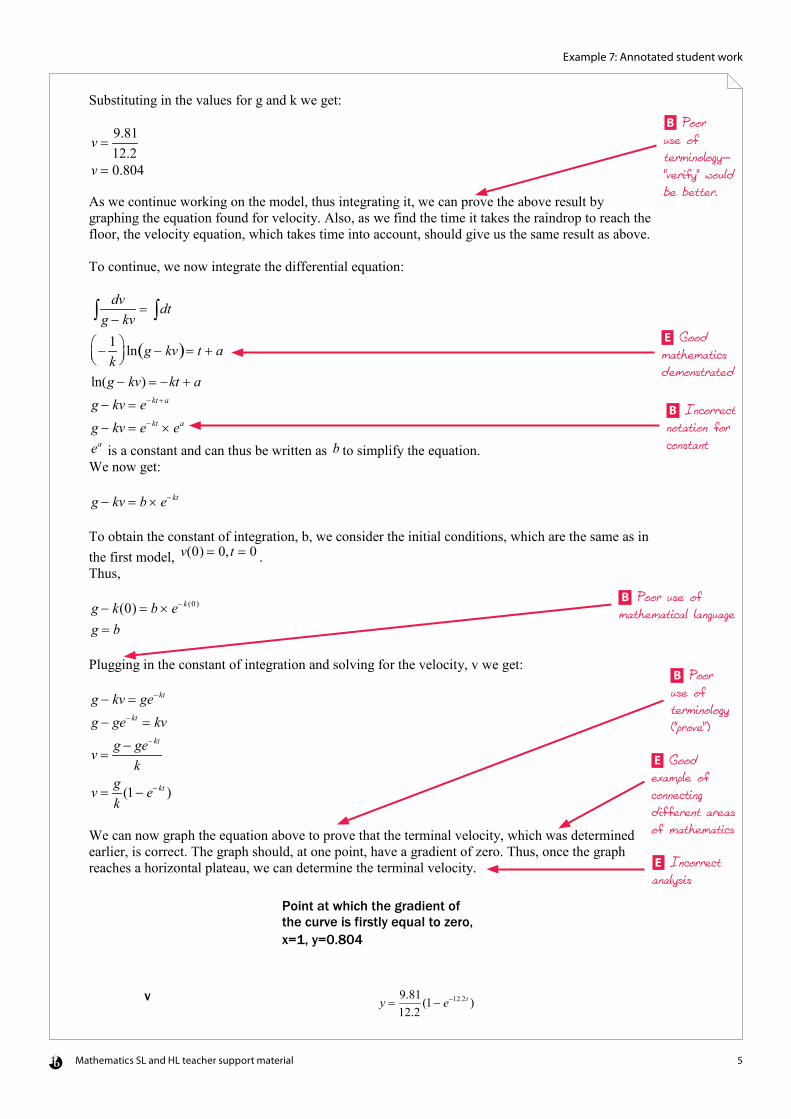
Mathematics SL and HL teacher support material 5
Example 7: Annotated student work
Substituting in the values for g and k we get:
v = 9.8112.2
v = 0.804 As we continue working on the model, thus integrating it, we can prove the above result by graphing the equation found for velocity. Also, as we find the time it takes the raindrop to reach the floor, the velocity equation, which takes time into account, should give us the same result as above. To continue, we now integrate the differential equation:
dvg − kv
= dt∫∫
−1k
ln g − kv( )= t + a
ln(g − kv) = −kt + ag − kv = e−kt+a
g − kv = e−kt × ea
ea is a constant and can thus be written as b to simplify the equation. We now get: g − kv = b × e−kt
To obtain the constant of integration, b, we consider the initial conditions, which are the same as in the first model, v(0) = 0,t = 0 . Thus, g − k(0) = b × e−k (0)
g = b Plugging in the constant of integration and solving for the velocity, v we get: g − kv = ge−kt
g − ge−kt = kv
v = g − ge−kt
k
v = gk
(1− e−kt )
We can now graph the equation above to prove that the terminal velocity, which was determined earlier, is correct. The graph should, at one point, have a gradient of zero. Thus, once the graph reaches a horizontal plateau, we can determine the terminal velocity.
y = 9.8112.2
(1− e−12.2t )
v
Point at which the gradient of the curve is firstly equal to zero, x=1, y=0.804
B Poor use of terminology—"verify" would be better.
E Good mathematics demonstrated
B Incorrect notation for constant
B Poor use of mathematical language
B Poor use of terminology ("prove")
E Good example of connecting different areas of mathematics
E Incorrect analysis
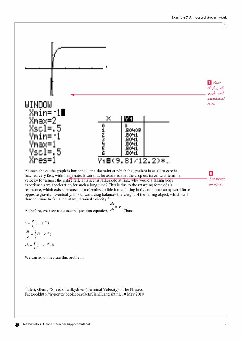
Mathematics SL and HL teacher support material 6
Example 7: Annotated student work
As seen above, the graph is horizontal, and the point at which the gradient is equal to zero is reached very fast, within a minute. It can thus be assumed that the droplets travel with terminal velocity for almost the entire fall. This seems rather odd at first, why would a falling body experience zero acceleration for such a long time? This is due to the retarding force of air resistance, which exists because air molecules collide into a falling body and create an upward force opposite gravity. Eventually, this upward drag balances the weight of the falling object, which will thus continue to fall at constant, terminal velocity.5
As before, we now use a second position equation,
dsdt
= v. Thus:
v = gk
(1− e−kt )
dsdt
=gk
(1− e−kt )
ds = gk
(1− e−kt )dt
We can now integrate this problem:
5 Elert, Glenn, “Speed of a Skydiver (Terminal Velocity)“, The Physics Factbookhttp://hypertextbook.com/facts/JianHuang.shtml, 10 May 2010
t
B Poor display of graph and associated data
E Incorrect analysis
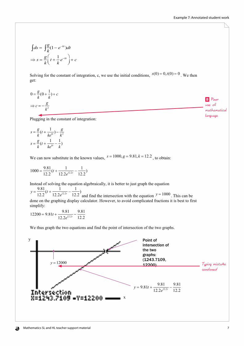
Mathematics SL and HL teacher support material 7
Example 7: Annotated student work
ds = gk∫∫ (1− e−kt )dt
⇒ s = gk
t + 1k
e−kt
+ c
Solving for the constant of integration, c, we use the initial conditions, s(0) = 0,t(0) = 0 . We then get:
0 =gk
(0 +1k
) + c
⇒ c = − gk2
Plugging in the constant of integration:
s = gk
(t + 1kekt ) −
gk2
s = gk
(t + 1kekt −
1k
)
We can now substitute in the known values, s = 1000,g = 9.81,k = 12.2 , to obtain:
1000 =9.8112.2
(t + 112.2e12.2t −
112.2
)
Instead of solving the equation algebraically, it is better to just graph the equation
y = 9.8112.2
(t + 112.2e12.2t −
112.2
)and find the intersection with the equation y = 1000 . This can be
done on the graphing display calculator. However, to avoid complicated fractions it is best to first simplify:
12200 = 9.81t + 9.8112.2e12.2t −
9.8112.2
We thus graph the two equations and find the point of intersection of the two graphs.
Point of intersection of the two graphs: (1243.7109, 12200) y = 12000
x
y
y = 9.81t + 9.8112.2e12.2t −
9.8112.2
B Poor use of mathematical language
Typing mistake condoned
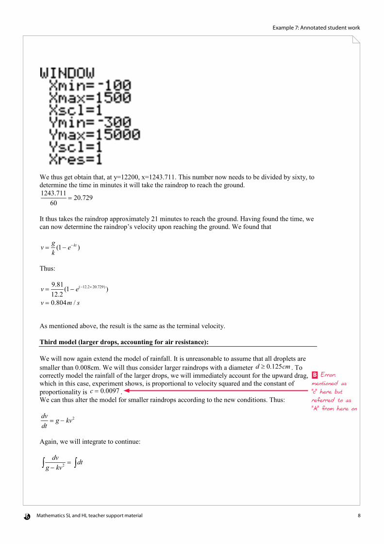
Mathematics SL and HL teacher support material 8
Example 7: Annotated student work
We thus get obtain that, at y=12200, x=1243.711. This number now needs to be divided by sixty, to determine the time in minutes it will take the raindrop to reach the ground. 1243.711
60= 20.729
It thus takes the raindrop approximately 21 minutes to reach the ground. Having found the time, we can now determine the raindrop’s velocity upon reaching the ground. We found that
v = gk
(1− e−kt )
Thus:
v = 9.8112.2
(1− e(−12.2×20.729) )
v = 0.804m / s As mentioned above, the result is the same as the terminal velocity. Third model (larger drops, accounting for air resistance): We will now again extend the model of rainfall. It is unreasonable to assume that all droplets are smaller than 0.008cm. We will thus consider larger raindrops with a diameter d ≥ 0.125cm . To correctly model the rainfall of the larger drops, we will immediately account for the upward drag, which in this case, experiment shows, is proportional to velocity squared and the constant of proportionality is c = 0.0097 . We can thus alter the model for smaller raindrops according to the new conditions. Thus: dvdt
= g − kv2
Again, we will integrate to continue:
dvg − kv2 = dt∫∫
B Error: mentioned as "c" here but referred to as "k" from here on
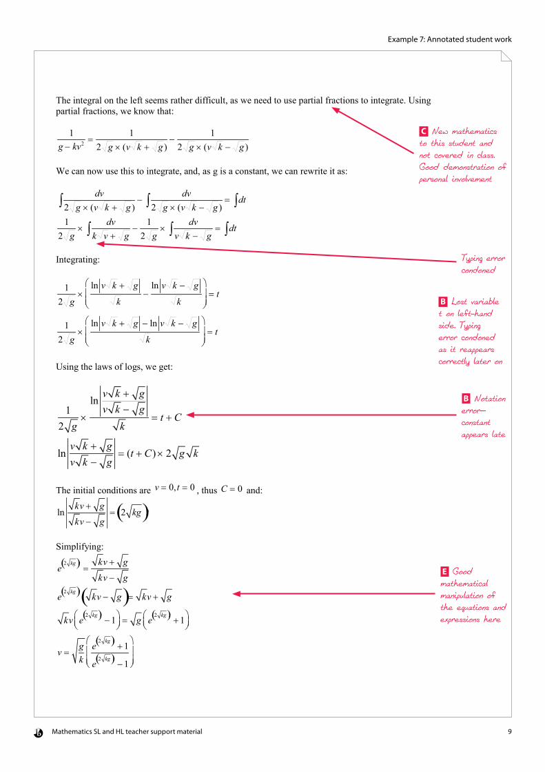
Mathematics SL and HL teacher support material 9
Example 7: Annotated student work
The integral on the left seems rather difficult, as we need to use partial fractions to integrate. Using partial fractions, we know that:
1g − kv2 =
12 g × (v k + g )
−1
2 g × (v k − g ) We can now use this to integrate, and, as g is a constant, we can rewrite it as:
dv2 g × (v k + g )∫ −
dv2 g × (v k − g )
= dt∫∫1
2 g×
dvk v + g∫ −
12 g
×dv
v k − g∫ = dt∫
Integrating:
12 g
×ln v k + g
k−
ln v k − g
k
= t
12 g
×ln v k + g − ln v k − g
k
= t
Using the laws of logs, we get:
12 g
×
lnv k + gv k − g
k= t + C
lnv k + gv k − g
= (t + C) × 2 g k
The initial conditions are v = 0,t = 0 , thus C = 0 and:
lnkv + g
kv − g= 2 kg( )t
Simplifying:
e2 kg( )t = kv + g
kv − g
e2 kg( )t kv − g( )= kv + g
kv e2 kg( )t −1
= g e
2 kg( )t +1
v = gk
e2 kg( )t +1
e2 kg( )t −1
C New mathematics to this student and not covered in class. Good demonstration of personal involvement
Typing error condoned
B Lost variable t on left-hand side. Typing error condoned as it reappears correctly later on
B Notation error—constant appears late
E Good mathematical manipulation of the equations and expressions here
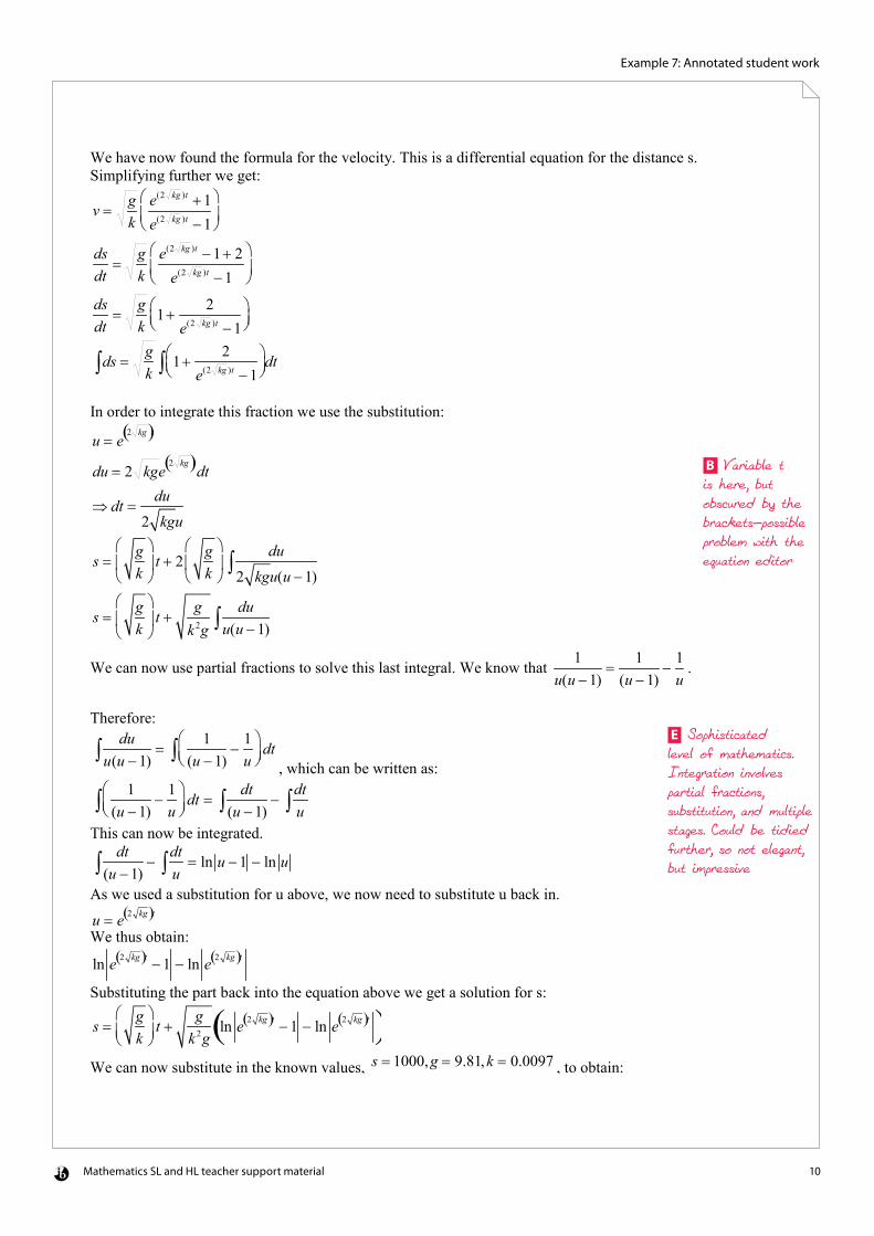
Mathematics SL and HL teacher support material 10
Example 7: Annotated student work
We have now found the formula for the velocity. This is a differential equation for the distance s. Simplifying further we get:
v = gk
e(2 kg )t +1e(2 kg )t −1
dsdt
=gk
e(2 kg )t −1+ 2e(2 kg )t −1
dsdt
=gk
1+2
e(2 kg )t −1
ds∫ =gk
1+2
e(2 kg )t −1
∫ dt
In order to integrate this fraction we use the substitution:
u = e2 kg( )t
du = 2 kge2 kg( )tdt
⇒ dt = du2 kgu
s = gk
t + 2
gk
du2 kgu(u −1)∫
s = gk
t + g
k2gdu
u(u −1)∫
We can now use partial fractions to solve this last integral. We know that 1u(u −1)
=1
(u −1)−
1u
.
Therefore:
duu(u −1)∫ =
1(u −1)
−1u
dt∫, which can be written as:
1(u −1)
−1u
dt∫ =dt
(u −1)∫ −dtu∫
This can now be integrated. dt
(u −1)∫ −dtu∫ = ln u −1 − ln u
As we used a substitution for u above, we now need to substitute u back in.
u = e 2 kg( )t We thus obtain:
ln e 2 kg( )t −1 − ln e 2 kg( )t
Substituting the part back into the equation above we get a solution for s:
s = gk
t + g
k2gln e 2 kg( )t −1 − ln e 2 kg( )t( )
We can now substitute in the known values, s = 1000,g = 9.81,k = 0.0097 , to obtain:
B Variable t is here, but obscured by the brackets—possible problem with the equation editor
E Sophisticated level of mathematics. Integration involves partial fractions, substitution, and multiple stages. Could be tidied further, so not elegant, but impressive
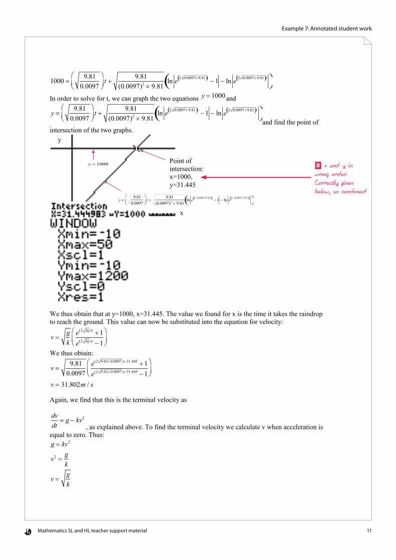
Mathematics SL and HL teacher support material 11
Example 7: Annotated student work
1000 =9.81
0.0097
t + 9.81
(0.0097)2 × 9.81ln e 2 0.0097×9.81( )t −1 − ln e 2 0.0097×9.81( )t( )
In order to solve for t, we can graph the two equations y = 1000 and
y = 9.810.0097
t + 9.81
(0.0097)2 × 9.81ln e 2 0.0097×9.81( )t −1 − ln e 2 0.0097×9.81( )t( )
and find the point of intersection of the two graphs.
We thus obtain that at y=1000, x=31.445. The value we found for x is the time it takes the raindrop to reach the ground. This value can now be substituted into the equation for velocity:
v = gk
e(2 kg )t +1e(2 kg )t −1
We thus obtain:
v = 9.810.0097
e(2 9.81×0.0097 )×31.445 +1e(2 9.81×0.0097 )×31.445 −1
v = 31.802m / s Again, we find that this is the terminal velocity as dvdt
= g − kv2
, as explained above. To find the terminal velocity we calculate v when acceleration is equal to zero. Thus: g = kv2
v2 =gk
v = gk
x
y
Point of intersection: x=1000, y=31.445
y = 1000
y = 9.810.0097
t + 9.81
(0.0097)2 × 9.81ln e 2 0.0097×9.81( )t −1 − ln e 2 0.0097×9.81( )t( )
B x and y in wrong order. Correctly given below, so condoned
Mathematics SL and HL teacher support material 12
Example 7: Annotated student work
v = 9.810.0097
v = 31.802 It is thus reasonable to assume that the large raindrops also travel at terminal velocity for most of the time. The Parachute Problem: To apply the concept of raindrop modelling to human beings, one could now consider a parachute jump. As I do not know much about skydiving, I first did some research around the basics of it. A typical parachute jump consists of the individuals jumping out of an aircraft at approximately 4,400 metres altitude. The period of free-fall takes about a minute, then the parachute is opened to slow the landing down, which takes between five and seven minutes. To model a parachute jump, we can say that the parachutist, just like any other falling object,
experiences constant acceleration g = 9.81ms−2, wince all objects fall with the same rate of
acceleration regardless of their mass. We also need to account for air resistance and can thus use the same model as before, when modelling the fall of small raindrops.
a =dvdt
dvdt
= g − kv
However, as the size of humans is not comparable to the size of small raindrops, we need to find a different value for k, as the air resistance is not the same in this case. Also, the significance of air resistance will ultimately depend on the position of the skydiver in the air. For example, a skydiver in the spread eagle position will encounter more air resistance than a parachutist, who falls feet or head first, which related back to the cross sectional area of the falling object as explained earlier. As explained earlier, the amount of air resistance is subject to change throughout the free fall, as it is also dependent upon speed. The air resistance is small at the start of the jump and the parachutist accelerates downward. As the speed of the free faller increases, the amount of air resistance goes up as well, thus slowing down acceleration. The air resistance force will eventually be equal and opposite to the downward force due to gravity and at this point the skydiver’s speed remains constant. Terminal velocity has thus been reached.6 In order to develop a model for the parachute problem, one would thus have to divide the free fall into three parts, each with a different amount of air resistance and then also develop a model for the slow descent after the parachute is deployed. The mathematical process however is very simple and the same as in the second model for small raindrops, k is just exchanged for the respective values of the air resistance, that is the constant of proportionality in reference to velocity. Having extended the mathematical exploration to the problem of a parachute jump, one can now critically reflect upon the work done. We can start by looking at the first model, which merely looks at raindrops as falling objects. It is an unrealistic model as such, as it does not account for air
6 „KS§ 9K Air resistance and friction“, slideshare, <http://www.slideshare.net/scienceinteractive/ks3-9k-air-resistance-and-friction>, 23 May 2010
Typing error
D Meaningful reflection
A Good conclusion

Mathematics SL and HL teacher support material 13
Example 7: Annotated student work
resistance. The results could thus be used as a rough idea on how to develop the other models, but other than that, were hypothetical. The second model, which looks at smaller raindrops, takes air resistance into account and thus gets a lot closer to reality. However, there are certain uncertainties to this model. To begin, we put all raindrops with a diameter smaller that 0.008cm into one group, the results are thus not specific to the respective size of the raindrop. In addition, we made the assumption that the amount of air resistance is always that same. In reality, the amount of air resistance is subject to a number of factors. As stated earlier, it depends upon the cross sectional area and speed of the object and thus changes throughout the fall. However, this is only a minor inaccuracy, as we found out that raindrops reach terminal velocity after a very short period of time and thus travel at terminal velocity, and thus the same speed, for almost the entire fall. The air resistance, however, can also be influenced by environmental factors, such as a strong wind. These uncertainties are the same for the third model, looking at larger raindrops. Bibliography: Elert, Glenn. "Speed of a Skydiver (Terminal Velocity)." The Physics Factbook. Web. 10 May
2010. <http://hypertextbook.com/facts/JianHuang.shtml>. Emerson, Brandon. "Raindrop Modeling." 2005. Web. 28 Apr. 2010.
<bpemer.people.wm.edu/Raindrops.doc>. "The Forces at Work - Gravity." Web. 22 May 2010. <http://ffden-
2.phys.uaf.edu/211.fall2000.web.projects/vlad%20paverman/forces.htm>. "Intensity of Rainfall." FLOODsite. Web. 07 May 2010.
<http://www.floodsite.net/juniorfloodsite/html/en/student/thingstoknow/hydrology/rainfallintensity.html>.
"KS3 9K Air Resistance and Friction." Slideshare. Web. 23 May 2010.
<http://www.slideshare.net/scienceinteractive/ks3-9k-air-resistance-and-friction>. Meade, Douglas B. "Ode Models for the Parachute Problem." Web. 16 May 2010.
<http://www.math.sc.edu/~meade/papers/sr-parachute.pdf>. Phoebus, Ronald, and Cole Reilly. "Differential Equations and the Parachute Problem." 10 May
2004. Web. 15 May 2010. <http://online.redwoods.cc.ca.us/instruct/darnold/DEProj/sp04/coleron/paper1.pdf>.
Smith, David A., and Lawrence C. Moore. "Raindrops." Math DL The MAA Mathematical Science
Digital Library. The Mathematical Association of America. Web. 05 May 2010. <http://mathdl.maa.org/mathDL/?pa=content&sa=viewDocument&nodeId=315&pf=1>.

Mathematics SL and HL teacher support material 14
Example 7: Annotated student work
"Student Project: Skydiving." Pure Mathematics 30. Alberta Education, Feb. 2009. Web. 18 May 2010. <http://education.alberta.ca/media/930712/03%20pure30%20feb-09%20skydiving%20student%20project_pdf%20final.pdf>.

solution she was after. Having supervised the student throughout the process, I can confirm thatthe student was very engaged with the task and all the work produced is her own.”
This information provided by the teacher justifies the levels awarded. Without this information,it may not be clear to others that the student was engaged and understood the work.
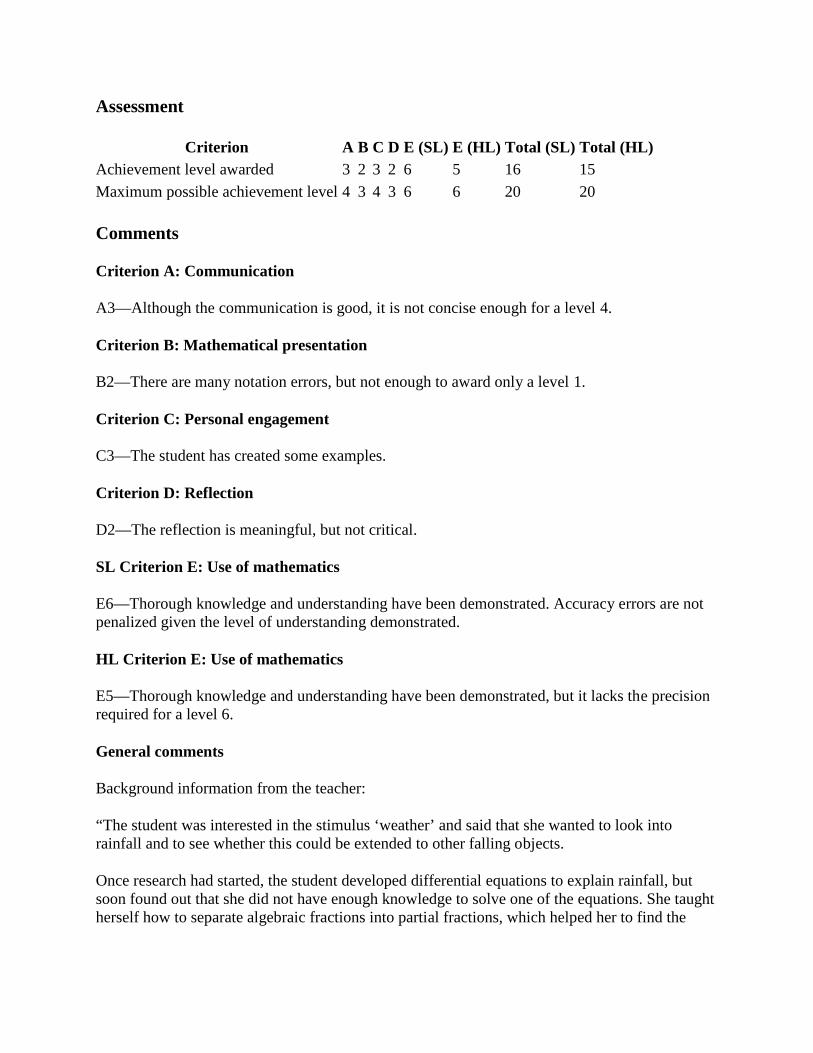
Assessment
Criterion A B C D E (SL) E (HL) Total (SL) Total (HL)Achievement level awarded 3 2 3 2 6 5 16 15
Maximum possible achievement level 4 3 4 3 6 6 20 20
Comments
Criterion A: Communication
A3—Although the communication is good, it is not concise enough for a level 4.
Criterion B: Mathematical presentation
B2—There are many notation errors, but not enough to award only a level 1.
Criterion C: Personal engagement
C3—The student has created some examples.
Criterion D: Reflection
D2—The reflection is meaningful, but not critical.
SL Criterion E: Use of mathematics
E6—Thorough knowledge and understanding have been demonstrated. Accuracy errors are notpenalized given the level of understanding demonstrated.
HL Criterion E: Use of mathematics
E5—Thorough knowledge and understanding have been demonstrated, but it lacks the precisionrequired for a level 6.
General comments
Background information from the teacher:
“The student was interested in the stimulus ‘weather’ and said that she wanted to look intorainfall and to see whether this could be extended to other falling objects.
Once research had started, the student developed differential equations to explain rainfall, butsoon found out that she did not have enough knowledge to solve one of the equations. She taughtherself how to separate algebraic fractions into partial fractions, which helped her to find the

solution she was after. Having supervised the student throughout the process, I can confirm thatthe student was very engaged with the task and all the work produced is her own.”
This information provided by the teacher justifies the levels awarded. Without this information,it may not be clear to others that the student was engaged and understood the work.