Naïve Bayes classification

1

Probability theory

Random variable: a variable whose possible values are numerical outcomes of a random phenomenon. Examples: A person’s height, the outcome of a coin toss Distinguish between discrete and continuous variables. The distribution of a discrete random variable: The probabilities of each value it can take. Notation: P(X = xi). These numbers satisfy:

2

X

i

P (X = xi) = 1

Probability theory

Marginal Probability Conditional Probability

Joint Probability

Probability theory

A joint probability distribution for two variables is a table. If the two variables are binary, how many parameters does it have? Let’s consider now the joint probability of d variables P(X1,…,Xd). How many parameters does it have if each variable is binary?

4

Probability theory

Marginalization:

Product Rule

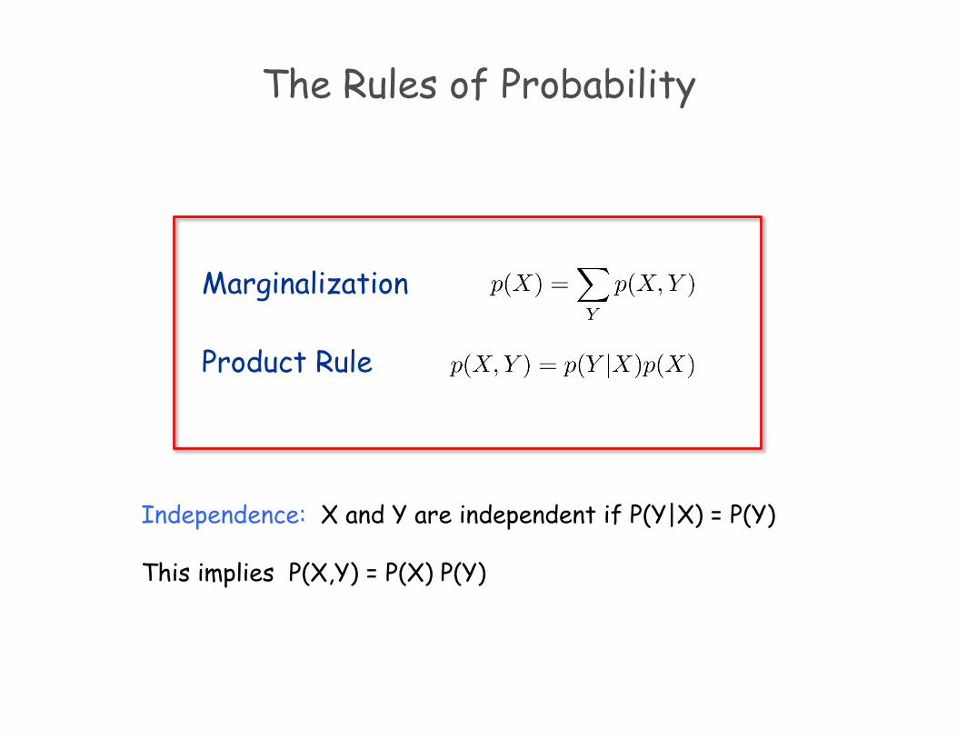
The Rules of Probability

Marginalization Product Rule

Independence: X and Y are independent if P(Y|X) = P(Y) This implies P(X,Y) = P(X) P(Y)

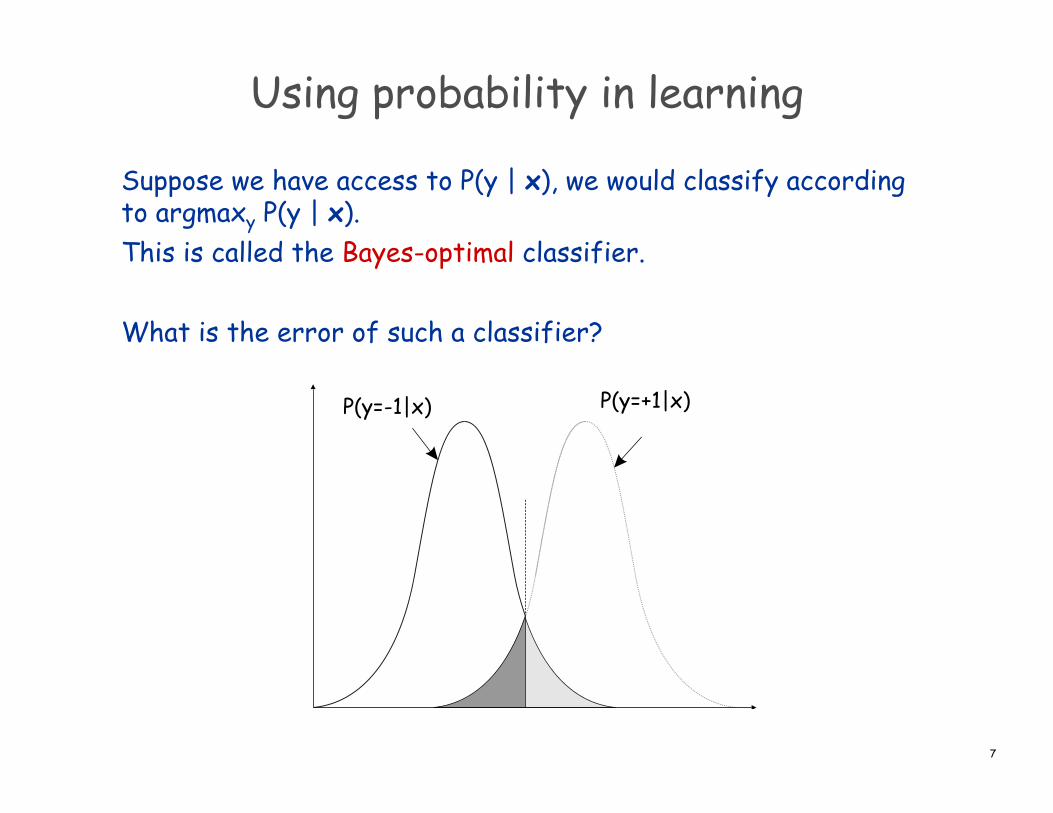
Using probability in learning

Suppose we have access to P(y | x), we would classify according to argmaxy P(y | x). This is called the Bayes-optimal classifier. What is the error of such a classifier?

7

J.Stat.M

ech.(2010)

P11015

A pattern recognition approach to complex networks

Figure 5. Example of the two regions R1 and R2 formed by the Bayesian classifierfor the case of two classes.

from the features of the classes known a priori. On the other hand, if the probabilitydensity function is not known initially, nonparametric estimation methods are necessary.These methods are variations of the histogram approximation technique for a probabilitydensity function. In the next subsections, we describe parametric and nonparametricclassification.

4.2.1. Parametric classification. In this method, the functional form of the probabilitydensity function is known or can be at least estimated. In most cases, each classof observations (e.g. network models) presents a Gaussian like distribution in the d-dimensional feature space, defined by a set of d measurements. In this way, the datadistribution for a given class c is described by

Pc(!x) =1

(2")d|!|1/2exp

!!1

2(!x ! !µc)

T !!1(!x ! !µc)

", (19)

where !µ is the d-dimensional average vector !µ = E [!x], E is the expectation [26], and ! isthe d " d covariance matrix, given by

! = E [(!x ! !µ)(!x ! !µ)T ], (20)

which is symmetric and has d(d + 1)/2 independent components. The term inside themultivariate normal density is the Mahalanobis distance, " = (!x ! !µ)T !!1(!x ! !µ), from!x to !µ.

The first step for the parametric classification is to compute the average of eachmeasurement for all elements of each class c and the respective covariance matrix, whichare used to estimate Pc. The classification is performed considering the decision ruledescribed above, i.e. for a given observation i (network, community or vertex), whosevector feature is !xi, the values Pc(!xi) are calculated for each class c. Then, the observationi is associated to the class with the largest probability. It should be noticed that theclassification can be performed in the original space or the projections obtained by the

doi:10.1088/1742-5468/2010/11/P11015 14

P(y=+1|x) P(y=-1|x)

Using probability in learning

Some classifiers model P(Y | X) directly: discriminative learning However, it’s usually easier to model P(X | Y) from which we can get P(Y | X) using Bayes rule: This is called generative learning

8

Op)mal&Classifica)on&Optimal predictor: (Bayes classifier)

3%

0%

0.5%

1%

Equivalently,%

P (Y |X) =P (X|Y )P (Y )

P (X)

Maximum likelihood

Fit a probabilistic model P(x | θ) to data   Estimate θ

Given independent identically distributed (i.i.d.) data X = (x1, x2, …, xn)   Likelihood

  Log likelihood

Maximum likelihood solution: parameters θ that maximize ln P(X | θ)

lnP (X|✓) =nX

i=1

lnP (xi|✓)

P (X|✓) = P (x1|✓)P (x2|✓), . . . , P (xn|✓)

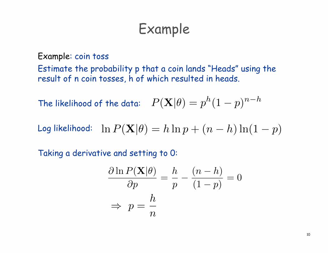
Example

Example: coin toss Estimate the probability p that a coin lands “Heads” using the result of n coin tosses, h of which resulted in heads. The likelihood of the data: Log likelihood: Taking a derivative and setting to 0:

10

P (X|✓) = ph(1� p)n�h

lnP (X|✓) = h ln p+ (n� h) ln(1� p)

@ lnP (X|✓)@p

=h

p� (n� h)

(1� p)= 0

) p =h

n

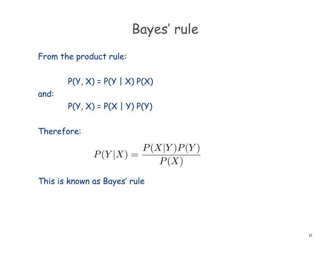
Bayes’ rule

From the product rule:

P(Y, X) = P(Y | X) P(X) and:

P(Y, X) = P(X | Y) P(Y) Therefore: This is known as Bayes’ rule

11

P (Y |X) =P (X|Y )P (Y )

P (X)

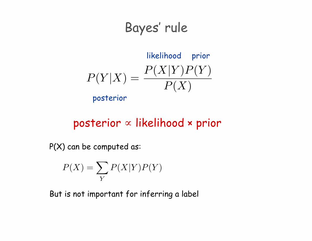
Bayes’ rule

posterior ∝ likelihood × prior

P (Y |X) =P (X|Y )P (Y )

P (X)posterior

prior

likelihood

P (X) =X

Y

P (X|Y )P (Y )

P(X) can be computed as: But is not important for inferring a label

Maximum a-posteriori and maximum likelihood

The maximum a posteriori (MAP) rule: If we ignore the prior distribution or assume it is uniform we obtain the maximum likelihood rule: A classifier that has access to P(Y|X) is a Bayes optimal classifier.

13

yMAP = argmax

YP (Y |X) = argmax

Y

P (X|Y )P (Y )

P (X)

= argmax

YP (X|Y )P (Y )

yML = argmax

YP (X|Y )

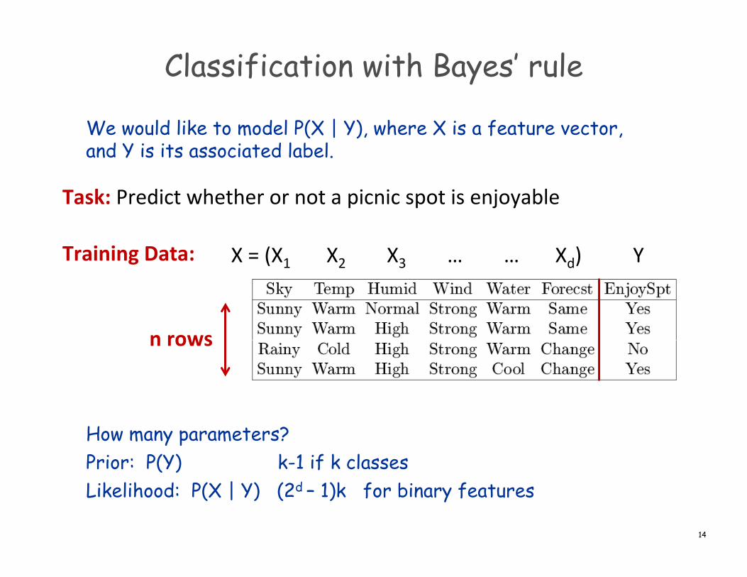
Classification with Bayes’ rule

We would like to model P(X | Y), where X is a feature vector, and Y is its associated label. How many parameters? Prior: P(Y) k-1 if k classes Likelihood: P(X | Y) (2d – 1)k for binary features

14

Learning&the&Op)mal&Classifier&Task:%Predict%whether%or%not%a%picnic%spot%is%enjoyable%%

Training&Data:&&

Lets&learn&P(Y|X)&–&how&many&parameters?&

9%

X%=%(X1%%%%%%%X2%%%%%%%%X3%%%%%%%%…%%%%%%%%…%%%%%%%Xd)%%%%%%%%%%Y%

Prior:%P(Y%=%y)%for%all%y% %%

Likelihood:%P(X=x|Y%=%y)%for%all%x,y %%

n&rows&

KR1&if&K&labels&

(2d&–&1)K&if&d&binary&features%

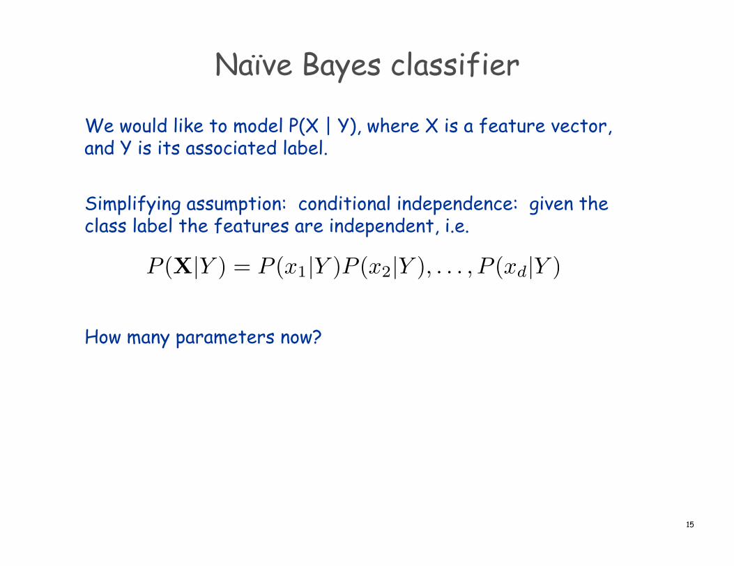
Naïve Bayes classifier

We would like to model P(X | Y), where X is a feature vector, and Y is its associated label. Simplifying assumption: conditional independence: given the class label the features are independent, i.e. How many parameters now?

15

P (X|Y ) = P (x1|Y )P (x2|Y ), . . . , P (xd|Y )

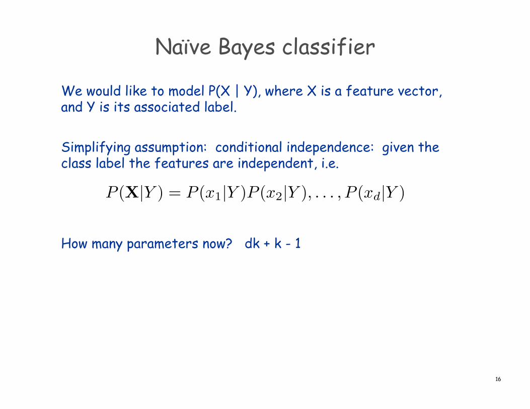
Naïve Bayes classifier

We would like to model P(X | Y), where X is a feature vector, and Y is its associated label. Simplifying assumption: conditional independence: given the class label the features are independent, i.e. How many parameters now? dk + k - 1

16

P (X|Y ) = P (x1|Y )P (x2|Y ), . . . , P (xd|Y )

Naïve Bayes classifier

Naïve Bayes decision rule: If conditional independence holds, NB is an optimal classifier!

17

yNB = argmax

YP (X|Y )P (Y ) = argmax

Y

dY

i=1

P (xi|Y )P (Y )

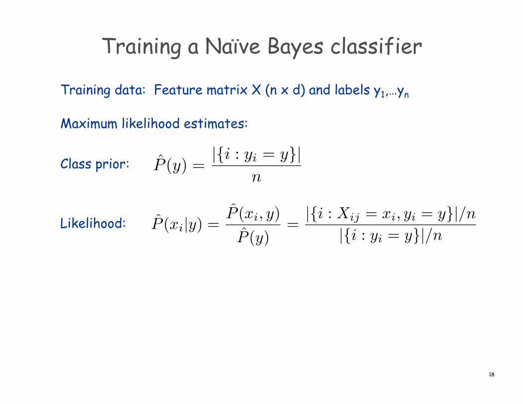
Training a Naïve Bayes classifier

Training data: Feature matrix X (n x d) and labels y1,…yn Maximum likelihood estimates: Class prior: Likelihood:

18

P̂ (y) =|{i : yi = y}|

n

P̂ (xi|y) =P̂ (xi, y)

P̂ (y)=

|{i : Xij = xi, yi = y}|/n|{i : yi = y}|/n

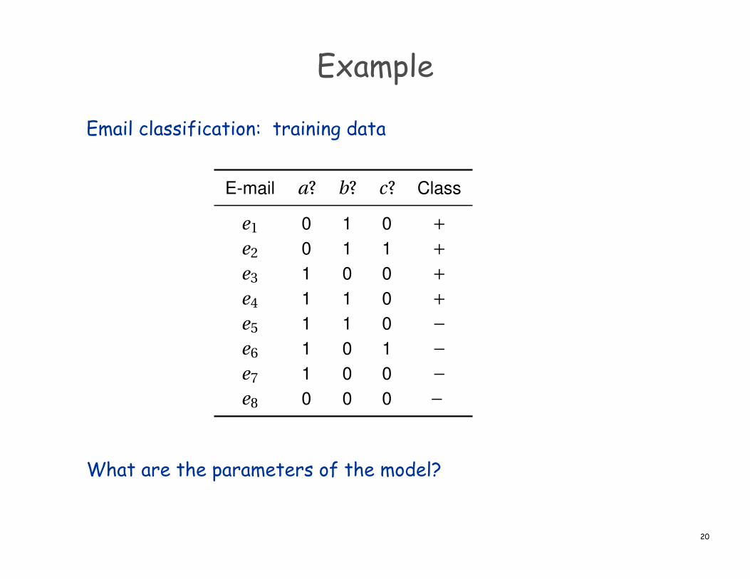
Example

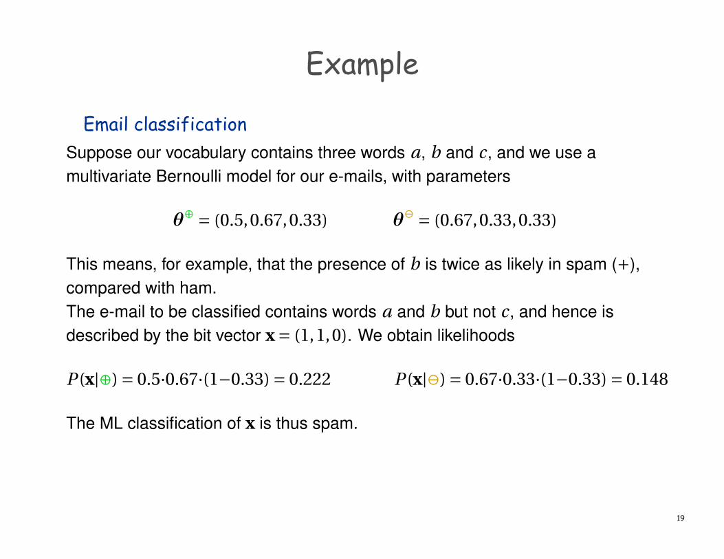
Email classification

19

9. Probabilistic models 9.2 Probabilistic models for categorical data

p.276 Example 9.4: Prediction using a naive Bayes model I

Suppose our vocabulary contains three words a, b and c, and we use amultivariate Bernoulli model for our e-mails, with parameters

✓© = (0.5,0.67,0.33) ✓™ = (0.67,0.33,0.33)

This means, for example, that the presence of b is twice as likely in spam (+),compared with ham.The e-mail to be classified contains words a and b but not c, and hence isdescribed by the bit vector x = (1,1,0). We obtain likelihoods

P (x|©) = 0.5·0.67·(1°0.33) = 0.222 P (x|™) = 0.67·0.33·(1°0.33) = 0.148

The ML classification of x is thus spam.

Peter Flach (University of Bristol) Machine Learning: Making Sense of Data August 25, 2012 273 / 349

Example

Email classification: training data What are the parameters of the model?

20

9. Probabilistic models 9.2 Probabilistic models for categorical data

p.280 Table 9.1: Training data for naive Bayes

E-mail #a #b #c Class

e1 0 3 0 +e2 0 3 3 +e3 3 0 0 +e4 2 3 0 +e5 4 3 0 °e6 4 0 3 °e7 3 0 0 °e8 0 0 0 °

E-mail a? b? c? Class

e1 0 1 0 +e2 0 1 1 +e3 1 0 0 +e4 1 1 0 +e5 1 1 0 °e6 1 0 1 °e7 1 0 0 °e8 0 0 0 °

(left) A small e-mail data set described by count vectors. (right) The same data setdescribed by bit vectors.

Peter Flach (University of Bristol) Machine Learning: Making Sense of Data August 25, 2012 277 / 349

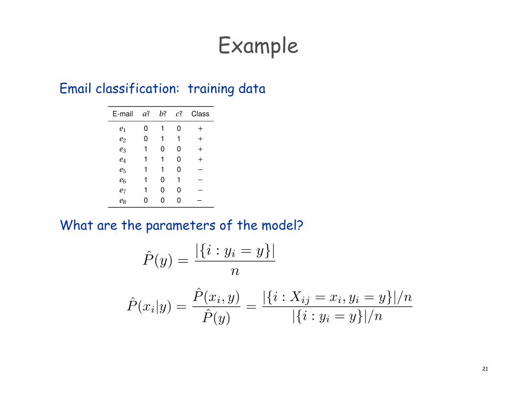
Example

Email classification: training data What are the parameters of the model?

21

9. Probabilistic models 9.2 Probabilistic models for categorical data

p.280 Table 9.1: Training data for naive Bayes

E-mail #a #b #c Class

e1 0 3 0 +e2 0 3 3 +e3 3 0 0 +e4 2 3 0 +e5 4 3 0 °e6 4 0 3 °e7 3 0 0 °e8 0 0 0 °

E-mail a? b? c? Class

e1 0 1 0 +e2 0 1 1 +e3 1 0 0 +e4 1 1 0 +e5 1 1 0 °e6 1 0 1 °e7 1 0 0 °e8 0 0 0 °

(left) A small e-mail data set described by count vectors. (right) The same data setdescribed by bit vectors.

Peter Flach (University of Bristol) Machine Learning: Making Sense of Data August 25, 2012 277 / 349

P̂ (y) =|{i : yi = y}|

n

P̂ (xi|y) =P̂ (xi, y)

P̂ (y)=

|{i : Xij = xi, yi = y}|/n|{i : yi = y}|/n

Example

Email classification: training data What are the parameters of the model? P(+) = 0.5, P(-) = 0.5 P(a|+) = 0.5, P(a|-) = 0.75 P(b|+) = 0.75, P(b|-)= 0.25 P(c|+) = 0.25, P(c|-)= 0.25

22

9. Probabilistic models 9.2 Probabilistic models for categorical data

p.280 Table 9.1: Training data for naive Bayes

E-mail #a #b #c Class

e1 0 3 0 +e2 0 3 3 +e3 3 0 0 +e4 2 3 0 +e5 4 3 0 °e6 4 0 3 °e7 3 0 0 °e8 0 0 0 °

E-mail a? b? c? Class

e1 0 1 0 +e2 0 1 1 +e3 1 0 0 +e4 1 1 0 +e5 1 1 0 °e6 1 0 1 °e7 1 0 0 °e8 0 0 0 °

(left) A small e-mail data set described by count vectors. (right) The same data setdescribed by bit vectors.

Peter Flach (University of Bristol) Machine Learning: Making Sense of Data August 25, 2012 277 / 349

P̂ (y) =|{i : yi = y}|

n

P̂ (xi|y) =P̂ (xi, y)

P̂ (y)=

|{i : Xij = xi, yi = y}|/n|{i : yi = y}|/n

Comments on Naïve Bayes

Usually features are not conditionally independent, i.e. And yet, one of the most widely used classifiers. Easy to train! It often performs well even when the assumption is violated.

Domingos, P., & Pazzani, M. (1997). Beyond Independence: Conditions for the Optimality of the Simple Bayesian Classifier. Machine Learning. 29, 103-130.

23

P (X|Y ) 6= P (x1|Y )P (x2|Y ), . . . , P (xd|Y )

When there are few training examples

What if you never see a training example where x1=a when y=spam? P(x | spam) = P(a | spam) P(b | spam) P(c | spam) = 0 What to do?

24

When there are few training examples

What if you never see a training example where x1=a when y=spam? P(x | spam) = P(a | spam) P(b | spam) P(c | spam) = 0 What to do? Add “virtual” examples for which x1=a when y=spam.

25

Naïve Bayes for continuous variables

Need to talk about continuous distributions!

26

f (x)

x

Uniform

x1 x2

x

f (x) Normal/Gaussian

x1 x2

Continuous Probability Distributions

The probability of the random variable assuming a value within some given interval from x1 to x2 is defined to be the area under the graph of the probability density function between x1 and x2.

Expectations

Conditional expectation (discrete)

Approximate expectation (discrete and continuous)

Continuous variables Discrete variables

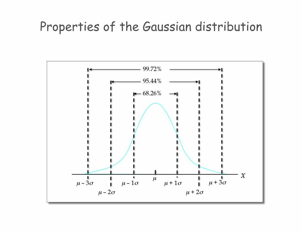
The Gaussian (normal) distribution

x µ – 3σ µ – 1σ

µ – 2σ µ + 1σ

µ + 2σ

µ + 3σ µ

68.26%

95.44%

99.72%

Properties of the Gaussian distribution

Standard Normal Distribution

A random variable having a normal distribution with a mean of 0 and a standard deviation of 1 is said to have a standard normal probability distribution.

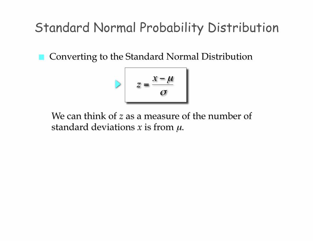
  Converting to the Standard Normal Distribution

z x=

− µσ

We can think of z as a measure of the number of standard deviations x is from µ.

Standard Normal Probability Distribution

Gaussian Parameter Estimation

Likelihood function

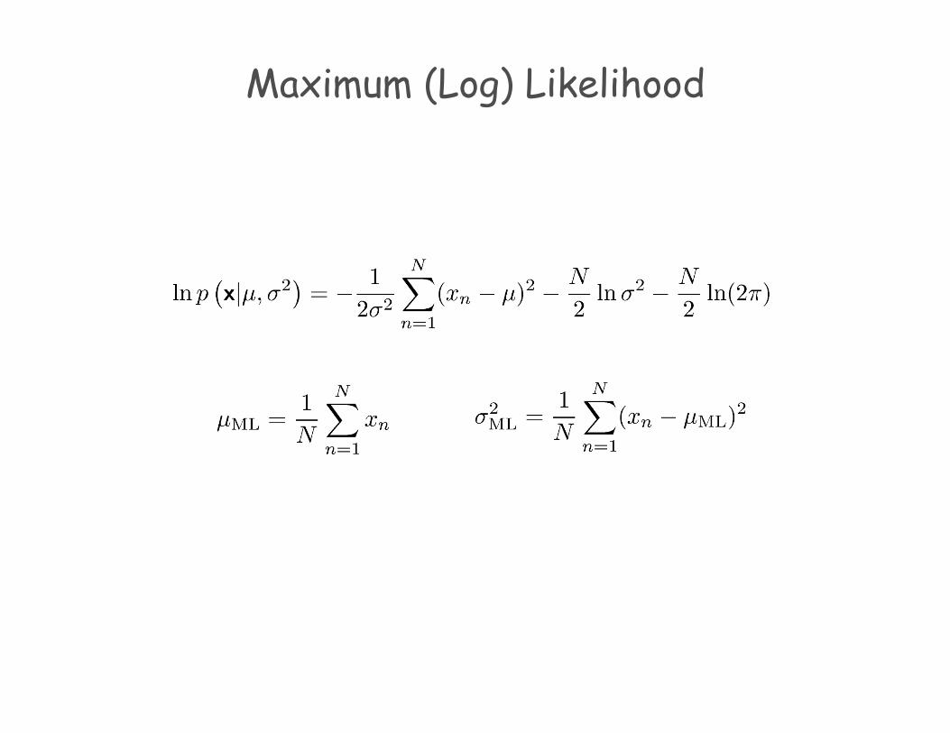
Maximum (Log) Likelihood

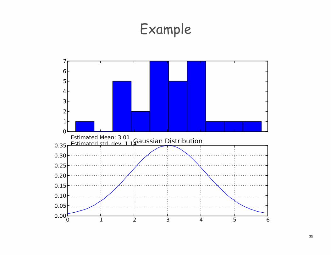
Example

35

Gaussian models

Assume we have data that belongs to three classes, and assume a likelihood that follows a Gaussian distribution

36

Gaussian Naïve Bayes

Likelihood function: Need to estimate mean and variance for each feature in each class.

37

P (Xi = x|Y = yk) =1p

2⇡�ik

exp

✓� (x� µik)

2

2�

2ik

◆

Summary

Naïve Bayes classifier: ²  What’s the assumption ²  Why we make it ²  How we learn it Naïve Bayes for discrete data Gaussian naïve Bayes

38