nano-indentation deformation studies of al-cu alloys via ... · nano-indentation deformation...
TRANSCRIPT
Nano-Indentation Deformation Studies of Al-Cu Alloys via Molecular
Dynamic Simulation
A Thesis submitted in partial fulfillment of the requirements for the
Degree
Of
Master of Technology (M. Tech) In
METALLURGICAL & MATERIALS ENGINEERING
By
PAUL PRAMOD LAKRA
(211MM1199)
Department of Metallurgical & Materials Engineering
National Institute of Technology
Rourkela-769008
2013
Nano-Indentation Deformation Studies of Al-Cu Alloys via Molecular
Dynamic Simulation
A Thesis submitted in partial fulfillment of the requirements for the
Degree
Of
Master of Technology (M. Tech)
In
METALLURGICAL & MATERIALS ENGINEERING
By
PAUL PRAMOD LAKRA (211MM1199)
Under the Guidance of
Prof. S. N. ALAM
And
Prof. N. YEDLA
Department of Metallurgical & Materials Engineering
National Institute of Technology
Rourkela-769008
2013
[i]
DEPARTMENT OF METALLURGICAL & MATERIALS
ENGINEERING
NATIONAL INSTITUTE OF
TECHNOLOGY ROURKELA-769008,
INDIA
CERTIFICATE This is to certify that the project entitled “ Nano-Indentation Deformation Studies of
Al-Cu Alloy Via Molecular Dynamic Simulation ” submitted by Mr. PAUL PRAMOD
LAKRA(211MM1199) in partial fulfillments for the requirements for the award of
Master of Technology Degree in Metallurgical & Materials Engineering at National
Institute of Technology, Rourkela (Deemed University) is an authentic work carried
out by them under my supervision and guidance.
To the best of my knowledge, the matter embodied in the report has not been submitted to
any other University / Institute for the award of any Degree or Diploma.
Date: 22.05.2013 Prof. N. YEDLA
Department of Metallurgical & Materials Engineering
National Institute of Technology
Rourkela-769008
[ii]
AC K N O WLE D GE M EN T
I would like to thank NIT Rourkela for giving me the opportunity to use its resources
and work in such a challenging environment. First and foremost, I take this opportunity to
express my deep regards and sincere gratitude to my guides Prof. S .N.Alam and
Prof. N. Yedla for his able guidance and constant encouragement during my project
work. This project would not have been possible without their help and the valuable time
that they have given me amidst their busy schedule.
I would also like to express my utmost gratitude to Prof. B.C Ray, HOD, Metallurgical
& Materials Engineering for allowing me to use the departmental facilities.
I would also like to extend my hearty gratitude to my friends and senior students of
this department who have always encouraged and supported in doing my work. Last but not
the least, I would like to thank all the staff members of Department of Metallurgical
&Materials Engineering who have been very cooperative with me.
Place: NIT-Rourkela Paul Pramod Lakra
Date: 22.05.201

[iii]
List of Symbols
K Kelvin
Tg onset of glass transition
Tx onset of crystallization
g(r) Radial distribution function
r radius
Å Angstrom
k Boltzmann constant
mi Mass of atom ‘i’
Fxi force acting on atom ‘i’ in X-direction
ri position vector of atom ‘i’
rj position vector of atom ‘j’
U(dij) Interaction potential between atoms ‘i’ and ‘j’
dij Distance between atom ‘i’ and atom ‘j’
Ei Total energy of atom ‘i’
t time
nN nano Newton
N number of particles/atoms
m particle mass
v root-mean square velocity

[iv]
ABSTRACT
This thesis is concerned with the modeling and simulation deformation studies of
crystalline Al-Cu (Al50-70:Cu30-50) alloys by classical molecular dynamic simulations (MD).
Deformation studies were done by nano-indentation by coding in LAMMPS (Large Scale
Atomic/Molecular Massively Parallel Simulator) which is a well studied and widely used
open source code. In this study the effect of temperature, indenter diameter, loading rate,
composition on mechanical properties of alloys have been investigated.
The simulated deformation studies were carried out by nano-indentation at room
temperature as well as at elevated temperatures (300 K and 500 K). Also the effect of Cu on
the deformation behavior was studied by varying copper content in the range of 15-25 at%.
The simulation box size of dimension (100 Ǻ×100Ǻ×100 Ǻ) and consisting of 62500 atoms
were used for all the alloys. In this study NVT ensemble with periodic boundary conditions
along the non-loading directions was used. It has been found that with increase in copper
content the strength of the alloy increased. Further, with increase of loading rate from 1 Å/ps
to 2 Å/ps the load increases as there is no sufficient time for atomic rearrangements. Also,
with increase in indenter diameter from 15 Å to 20 Å hardness increases, this is due to more
resistance offered by the atoms of the alloy to indentation. Furthermore, with increasing
temperature the hardness of the alloys decreased. The results obtained could lead to better
understanding the behavior of the alloys at the macroscopic level.
Keywords: Molecular dynamic, Nano-indentation, crystalline, Hardness.
[v]
List of Figures
Figure No. Description
Figure 2.1 Represent difference between crystalline and amorphous structure
Figure 2.2 Volume-temperature plots showing the relationships between liquid, glassy and
solid states
Figure 2.3 Nano indentations with spherical indenter
Figure 2.4 Schematic representation of a force displacement curve for loading and
unloading, indicating stiffness S as the slope of the unloading curve at peak
load, total displacement ht at peak load, and the residual deformation hr after
unloading
Figure 2.5 Shows with increasing cu content hardness of Al-Cu alloys increases
Figure 2.6 Shows extruded space frame BIW architecture, Al-Cu alloy -Audi A8.
Figure 2.7 The measuring chamber case.
Figure 2.8 Forged Al-Cu Wheel
Figure 4.1 Atomic arrangements in a crystalline material
Figure 4.2 (a) VMD snap shot of Al70-Cu30 crystalline alloy (b) RDF plot for Al70-Cu30
pair.
Figure 4.3 (a) VMD snap shot of Al67-Cu33 crystalline alloy (b) RDF plot for
Al67- Cu33 pair
Figure 4.4 (a) VMD snap shot of Al50-Cu50 crystalline alloy (b) RDF plot for Al50-Cu50
pair.
Figure 4.5 Time step vs. Temperature plot for (a) Al70-Cu30 (b) Al67-Cu and (c) Al50-Cu50
alloy.
[vi]
Figure 4.6 VMD snapshots of the alloy during indentation at different loading rates: a) 1
Å/ps; b) 2 Å/ps.
Figure 4.7 Load-displacement curves during indentation at different loading rates 1 Å/ps
and 2 Å/ps.
Figure 4.8 Temperature-time plots during indentation at 300 K
Figure 4.9 Load-displacement curves during indentation at different temperature during
loading rate of 2 Å/ps.
Figure 4.10 Load-displacement curves during indentation at different indenter diameters
(15 Å and 20 Å) during loading rate of 1 Å/ps and 300 K.
Figure 4.11 Load-displacement curves during indentation at different indenter diameters
(15 Å and 20 Å) during loading rate of 2 Å/ps and 300 K.
Figure 4.12 Load-displacement plot of the alloy during different indenter diameter at 500
K and loading rate of (a) 1 Å/ps and (b) 2 Å/ps.
Figure 4.13 VMD snapshots of the alloy during indentation at different loading rates a) 1
Å/ps; b) 2 Å/ps.
Figure 4.14 Load-displacement curves during indentation at different loading rates 1 Å/
and 2 Å/ps.
Figure 4.15 Temperature-time plots during indentation at 300 K.
Figure 4.16 Load-displacement curves during indentation at different temperature during
loading rate of 2 Å/ps with different indenter diameters.
Figure 4.17 Load-displacement curves during indentation at different indenter diameters
(15 Å and 20 Å) during loading rate of 1 Å/ps and 300 K.
Figure 4.18 Load-displacement curves during indentation at different indenter diameters
(15 Å and 20 Å) during loading rate of 2 Å/ps and at 300 K.
Figure4.19 shows the load-displacement plot of the alloy during different indenter
diameter at 500 K and loading rate of 1 Å/ps and 2 Å/ps
Figure 4.20 VMD snapshots of the alloy during indentation at different loading rates a)
1Å/ps; b) 2 Å/ps.
Figure 4.21 Load-displacement curves during indentation at different loading rate 1 Å/ps
and 2 Å/ps.
[vii]
Figure 4.22 Temperature-time plot during indentation at 300 K
Figure 4.23 Load-displacement curves during indentation at different temperature during
loading rate of 2 Å/ps with indenters of different diameters: a) 15 Å b) 20 Å.
Figure 4.24 Load-displacement curves during indentation at different indenter diameters
(15 Å and 20 Å) during loading rate of 1 Å/ps and 300 K.
Figure 4.25 Load-displacement curves during indentation at different indenter diameters
(15 Å and 20 Å) during loading rate of 2 Å/ps and 300 K.
Figure 4.26 Load-displacement plot of the alloy during different indenter diameter at 500
K and loading rate of 1 Å/ps and 2 Å/ps.
Figure 4.27 Load-displacement plots of the alloys at 300 K and different loading rates
(a) 1 Å/ps and (b) 2 Å/ps
Figure 4.28 Load-displacement plots of the alloys at 500 K and different loading rates i.e.
(a) 1 Å/ps and (b) 2 Å/ps.

[viii]
Contents
Page no.
Certificate i
Acknowledgements ii
List of symbols iii
Abstract iv
List of Figure v-vii
Contents viii-xi
Chapter 1 Introduction
1.1 Background 1
1.2 Motivation for the present study 2
1.3 Key objective 2
1.4 Organization of thesis 2
Chapter 2 Literature Review
2.1 Background 3
2.2 Formation of crystalline state 3
2.3 Crystalline solid 4
2.4 Properties of crystalline materials 5
2.5 MD simulation historical background 5
2.6 Applications of MD simulation 6
2.7 Nano-indentation 6-8
2.8 Spherical indenter 8-9
2.9 Details about Al-Cu alloy 9
2.10 Properties of Al-Cu alloys 10
[ix]
2.10.1 Microhardness 10
2.10.2 Grain size, impact energy, flow stress and mechanical characteristics 11
2.11 Application of Al-Cu alloys 11-13
Chapter 3 Procedure of Classical Molecular Dynamic Simulation
3.1 Introduction 14
3.2 Interatomic potential 14
3.3 Potentials MD simulations 15
3.3.1 Embedded atom method (EAM) 15
3.3.2 Empirical Potentials 15
3.3.3 Pair wise Potentials & Many-Body Potentials 15
3.3.4 Semi-Empirical Potentials 16
3.3.5 Polarizable potential 16
3.4 Ab-initio Quantum-Mechanical Methods 16-17
3.5 Simulation method in Molecular dynamics 17-18
3.6 General steps of molecular dynamics simulation 18
3.7 Periodic boundary condition 18
3.8 Ensembles 18
3.9 Calculation of Temperature 18
3.10 Introduction to LAMMPS (Large-scale Atomic/Molecular Massively Parallel 19
Simulator)
3.10.1 Background 19
3.10.2 General features 19
3.10.3 Force fields 19
3.10.4 Atoms creation 19
3.10.5 Ensembles, constraints, and boundary conditions 20
3.10.6 Boundary conditions 20
[x]
3.10.7 Integrator 20
3.10.8 Energy minimization 20
3.10.9 LAMMPS input script 20-21
3.11 Output 21-22
3.12 Simulation studies performed using LAMMPS 22
3.13 Visual Molecular dynamics (VMD) 22
Chapter 4 Results and discussions
4.1 Creation of Al-Cu Crystalline alloy 23
4.2 Radial Distribution Function (RDF) 23
4.3 Time step vs. Temperature plots 24-25
4.4 Indentation studies 26
4.4.1 Indentation studies of model Al70-Cu30 alloy 26
4.4.2 Effect of loading rate 26-27
4.4.3 Effect of Temperature 27-28
4.4.4 Effect of Indentation diameter 28-30
4.5 Indentation studies of model Al67-Cu33 alloy 30
4.5.1 Effect of loading rate 30-31
4.5.2 Effect of Temperature 32
4.5.3 Effect of Indentation diameter 33-34
4.6 Indentation studies of model Al50-Cu50 alloy 34
4.6.1 Effect of loading rate 34-35
4.6.2 Effect of Temperature 36
4.6.3 Effect of Indentation diameter 37
4.7 Effect of composition 38-39

[xi]
Chapter 5 Conclusion and Scope for future work
5.1 Conclusions 40
5.2 Scope for future work 40
Chapter 6 References

CHAPTER 1
INTRODUCTION
[1]
CHAPTER 1
INTRODUCTION
1.1 Back ground
In recent years considerable use has been made of large digital computers to study
various aspects of molecular dynamic in solids, liquids, and gases [1]. The atomic
arrangement or crystalline structure of a material is important in determining the behavior
and properties of a solid material. Aluminum is the second widely used metal due to its
desirable chemical, physical and mechanical properties and it represents an important
category of technological materials. Due to its high strength-to weight ratio, besides other
desirable properties e.g. desirable appearance, non-toxic, non-sparking, nonmagnetic, high
corrosion resistance, high electrical and thermal conductivities and ease of fabrication,
aluminum and its alloys are used in a wide range of industrial applications for different
aqueous solutions. These properties led also to the association of aluminum and its alloys
with transportation particularly with aircraft and space vehicles, construction and building,
containers and packaging and electrical transmission lines [2].
In our study the method of molecular dynamics is applied to calculate the mechanical
properties of Al-Cu alloys. One of the main peculiarities of the classical molecular dynamics
is a choice of model potentials of inter atomic interaction, especially when metal systems are
under consideration. We used the embedded atom method (EAM) based on the potential,
which consists of many-body contribution to the interaction taking into account atomic
density distribution. On the other hand the EAM can be easily combined with the molecular
dynamics method and it is proved to give highly reliable results for a number of pure liquid
metals and some alloys [3]. All strengthening techniques rely on simple principal; restricting
or hindering dislocation motion which renders the material harder and stronger. The
strengthening mechanisms can be introduced by solid solution, strain hardening, precipitation
hardening and grain size reduction. Fine grain size is often desired for high strength. Fine
particles may be added to increase strength and phase transformations may also be utilized to
increase strength [4]. Mechanical properties of Al-Cu alloys depend on copper content.
Copper is generally added to aluminum alloys to increase their strength, hardness, fatigue and
creep resistances and mach-inability. The first and most widely used aluminum alloys were
those containing 4-10 wt. % Cu. On the other hand Al-Cu alloys, among the main aluminum
alloys, have the lowest negative potential of corrosion [5]. Copper is being used, because it is
[2]
one of the few elements that have relatively high solubility in Al. Thus, the product has an Al
(Cu) solid solution matrix that is mechanically tougher than a pure Al matrix [6].
1.2 Motivation of present studies
Al-Cu alloys are widely used in a light material production. Their practical
application is dictated by distinctive characteristics such as low density, high melting
temperature and a good thermal conductivity. In literature, one can find a variety of
experimental data related to these alloys, while there is a lack of computer simulation studies,
which could expand our knowledge about microscopic behavior in Al-Cu alloys [3].
1.3 Keys objective
a. To study the effect of composition on strength of Al-Cu alloys.
b. To study effect of loading rate on strength of Al-Cu alloys.
c. To study the effect of temperature on strength of Al-Cu alloys
d. To study the effect of indenter diameter on strength of Al-Cu alloys.
1.4 Organization of thesis
This chapter (Chapter 1) provides a brief introduction of the present work along with
its primary objectives and a brief look at the MD simulation studies on deformation of Al-Cu
crystalline alloys. Chapter 2 presents a literature review on the subject matter of crystalline
forming ability, historical background, properties of crystalline materials, nano-indentation
deformation studies effect of spherical indenter, details about Al alloys, properties of Al-Cu
alloys, MD simulation studies and application of Al-Cu alloys. Also gives brief explanation
of effect of loading rate, temperature, indenter diameter and composition on mechanical
properties of Al-Cu alloys. Chapter 3 gives a brief description of classical molecular
dynamics modeling, features of LAMMPS software and plan showing the details of
simulation studies. Chapter 4 describes Creation of Al-Cu Crystalline alloy with Radial
Distribution Function (RDF). Further it shows Time step vs. Temperature plots for stabilized
at room temperature. Then it describes Indentation studies of the entire alloys model to know
the effect of loading rate, effect of Temperature and effect of Indentation diameter on
strength of alloys. At last it shows the effect of composition. Chapter 5 presents the
conclusions of this study and scope for future work.

CHAPTER 2 Literature review
[3]
CHAPTER 2
LITERATURE REVIEW
2.1 Back ground
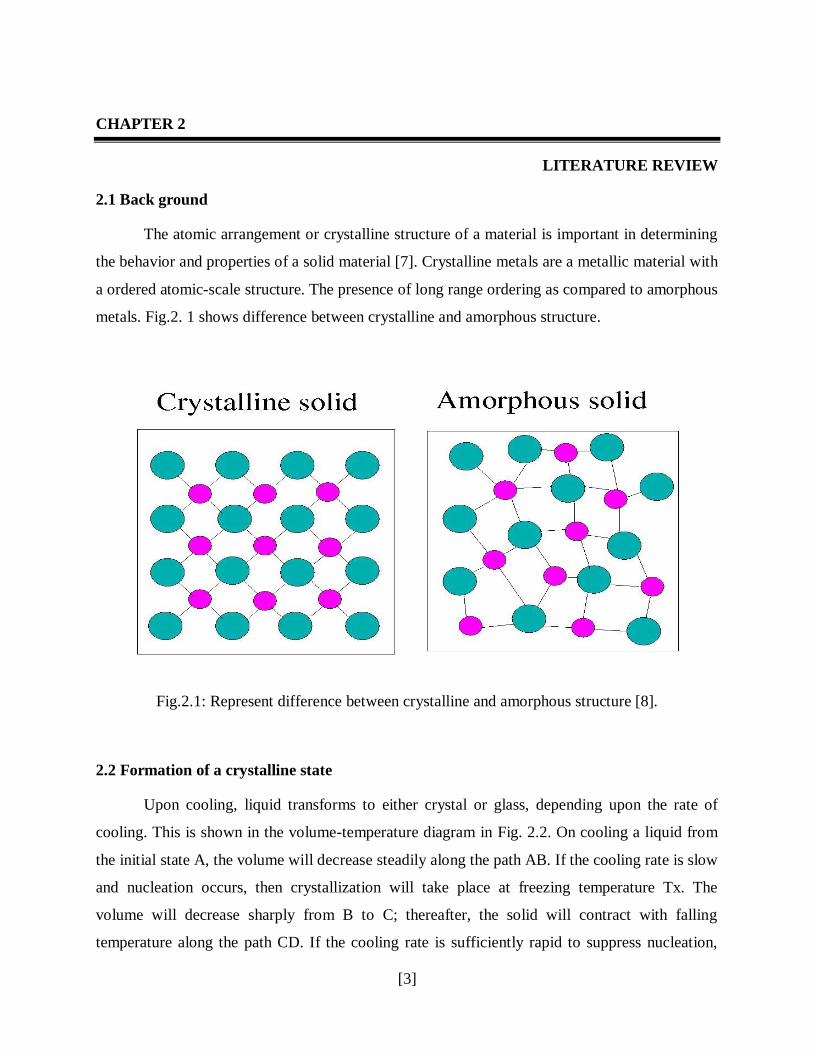
The atomic arrangement or crystalline structure of a material is important in determining
the behavior and properties of a solid material [7]. Crystalline metals are a metallic material with
a ordered atomic-scale structure. The presence of long range ordering as compared to amorphous
metals. Fig.2. 1 shows difference between crystalline and amorphous structure.
Fig.2.1: Represent difference between crystalline and amorphous structure [8].
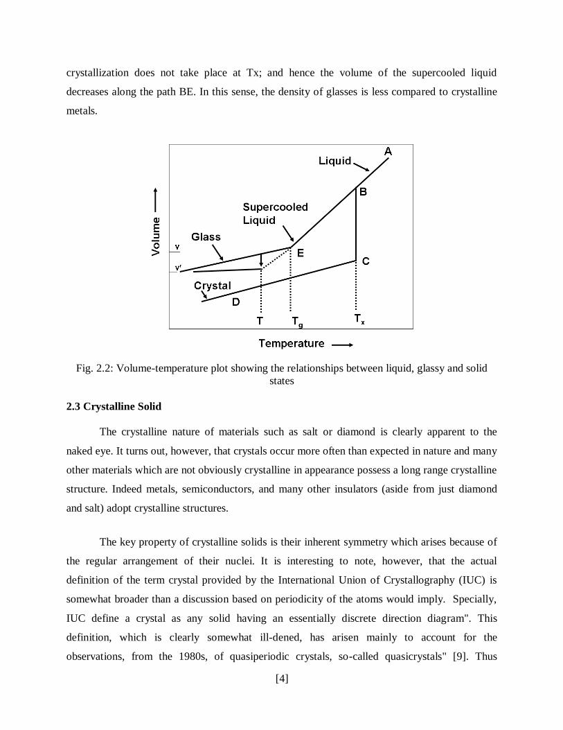
2.2 Formation of a crystalline state
Upon cooling, liquid transforms to either crystal or glass, depending upon the rate of
cooling. This is shown in the volume-temperature diagram in Fig. 2.2. On cooling a liquid from
the initial state A, the volume will decrease steadily along the path AB. If the cooling rate is slow
and nucleation occurs, then crystallization will take place at freezing temperature Tx. The
volume will decrease sharply from B to C; thereafter, the solid will contract with falling
temperature along the path CD. If the cooling rate is sufficiently rapid to suppress nucleation,
[4]
crystallization does not take place at Tx; and hence the volume of the supercooled liquid
decreases along the path BE. In this sense, the density of glasses is less compared to crystalline
metals.
Fig. 2.2: Volume-temperature plot showing the relationships between liquid, glassy and solid
states
2.3 Crystalline Solid
The crystalline nature of materials such as salt or diamond is clearly apparent to the
naked eye. It turns out, however, that crystals occur more often than expected in nature and many
other materials which are not obviously crystalline in appearance possess a long range crystalline
structure. Indeed metals, semiconductors, and many other insulators (aside from just diamond
and salt) adopt crystalline structures.
The key property of crystalline solids is their inherent symmetry which arises because of
the regular arrangement of their nuclei. It is interesting to note, however, that the actual
definition of the term crystal provided by the International Union of Crystallography (IUC) is
somewhat broader than a discussion based on periodicity of the atoms would imply. Specially,
IUC define a crystal as any solid having an essentially discrete direction diagram". This
definition, which is clearly somewhat ill-dened, has arisen mainly to account for the
observations, from the 1980s, of quasiperiodic crystals, so-called quasicrystals" [9]. Thus
[5]
periodic crystals, which we will focus on here, are just a subset. How the nuclei are arranged
leads to the crystal structure which is the unique arrangement of atoms in a crystal composed of a
unit cell: a set of atoms arranged in a particular way which is periodically repeated in three
dimensions on a lattice. The unit cell is given in terms of its lattice parameters, the length of the
unit cell edges and the angles between them.
2.4 Properties of Crystalline Material
These solids have a particular three dimensional geometrical structure.
The arrangement order of the ions in crystalline solids is of long order. The strength of all the
bonds between different ions, molecules and atoms is equal. Melting point of crystalline solids is
extremely sharp. Mainly the reason is that the heating breaks the bonds at the same time [10].
The physical properties like thermal conductivity, electrical conductivity, refractive index
and mechanical strength of crystalline solids are different along different directions. These solids
are the most stable solids as compared to other solids.
2.5 MD simulation historical background
The molecular dynamics method was original introduced by Alder and Wainwright in the
late 1950’s to learn the interactions of hard spheres. Many significant insights concerning the
behavior of simple liquids emerged from their studies [11][12] . The next major advance was in
1964, when Rahman carried out the first simulation using a realistic potential for liquid argon
[13]. The first molecular dynamics simulation of a realistic system was done by Rahman and
Stillinger in their simulation of liquid water in 1974[14]. The first protein simulations appeared
in 1977 with the simulation of the bovine pancreatic trypsin inhibitor (BPTI) [15].
Today in the literature, one routinely finds molecular dynamics simulations of solvated
proteins, protein-DNA complexes as well as lipid systems addressing a variety of issues
including the thermodynamics of ligand binding and the folding of small proteins. The number
of simulation techniques has greatly expanded; there exist now many specialized techniques for
particular problems, including mixed quantum mechanical - classical simulations that are being
employed to study enzymatic reactions in the context of the full protein. Molecular dynamics
[6]
simulation techniques are widely used in experimental procedures such as X-ray crystallography
and NMR structure determination.
2.6 Applications of MD simulation [16]:
i. I t is mostly used for simulation of bio-molecular systems like protein synthesis and
characterization.
ii. Used for drugs designing in pharmaceutical industry to test properties of a molecule
without synthesizing it.
iii. Used to study the effect of neutrons and ion irradiation on solid surfaces.
iv. It has wide applications in materials sectors too where experiments regarding any
problem are very difficult to carry out in laboratory conditions.
v. It is also used to study various properties of metals, non-metals and alloys like fatigue
properties, tensile properties, deformation behavior, high temperature behavior etc.
2.7 Nano-Indentation
Nano-indentation has been shown to be a useful technique for characterizing the
mechanical properties of materials and thin films in particular [17-19]. Indentation technique was
for the first time introduced in XIX century. Primarily, indentation technique was used to
measure material hardness H. In history the indentation was done by indenters of various shapes
thus leading to a variety of tests and analytical definitions of the hardness value. Currently, the
indentation technique was enhanced in order to assess additionally basic mechanical properties,
which was elastic modulus E of the investigated material. The above indentation method was
introduced in the year 1992 and was named as nano-indentation [20]. Currently the indentation
technique was enhanced in order to address problems referring to nano-scale. The above
technique is referred to as nanoindentation [21]. It is an improvement of the traditional
indentation technique.
[7]
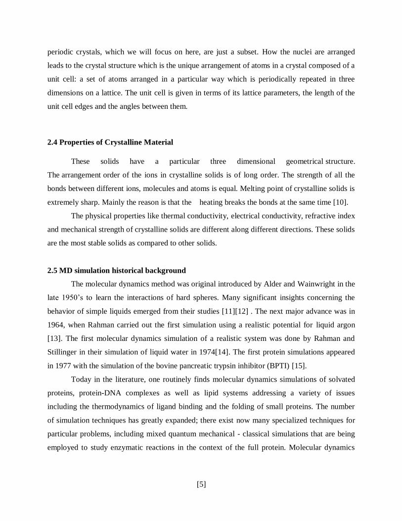
Fig.2.3: Nano indentation with spherical indenter[22]
Nano-indention is an experimental technique for measuring the hardness of materials on
the nanoscale and as such it can be used to measure the properties of thin films and
nanoparticulate materials. A sharp tip attached to the end of a cantilever is pushed into the
material and the required force is measured as a function of the depth the tip is pushed in. From
this both the material's hardness and its Young's modulus can be measured. On retraction of the
tip from the material any piling up of material around the hole made by the indenter can be
studied. This gives some insight into the nature of the atomistic processes taking place in the
sample. Although the technique is becoming established as a useful experimental methodology
for the measurement of the properties of materials on the nanoscale little is known about the
atomistic processes that take place during the nano- indentation process. These can be elucidated
through the use of modeling and to this goal we have modeled the nano-indentation process
using molecular dynamics (MD), describing both the tip and the sample automatically [23]. This
has allowed us to study the important atomistic processes that take place during the indentation
and the retraction of the tip. They have used this approach to study a number of systems
including Fe and Si experiments has shown that the model is able to pick up a number of
macroscopic features that are observed in the experiments and provide an explanation for these at
the atomic level [24].
[8]
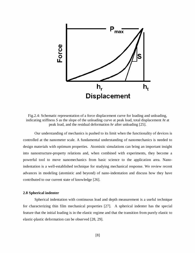
Fig.2.4: Schematic representation of a force displacement curve for loading and unloading,
indicating stiffness S as the slope of the unloading curve at peak load, total displacement ht at
peak load, and the residual deformation hr after unloading [25].
Our understanding of mechanics is pushed to its limit when the functionality of devices is
controlled at the nanometer scale. A fundamental understanding of nanomechanics is needed to
design materials with optimum properties. Atomistic simulations can bring an important insight
into nanostructure-property relations and, when combined with experiments, they become a
powerful tool to move nanomechanics from basic science to the application area. Nano-
indentation is a well-established technique for studying mechanical response. We review recent
advances in modeling (atomistic and beyond) of nano-indentation and discuss how they have
contributed to our current state of knowledge [26].
2.8 Spherical indenter
Spherical indentation with continuous load and depth measurement is a useful technique
for characterizing thin film mechanical properties [27]. A spherical indenter has the special
feature that the initial loading is in the elastic regime and that the transition from purely elastic to
elastic-plastic deformation can be observed [28, 29].
[9]
The main advantages of indentation with spherical indenters are:
1) Possibility of measurement under low stresses so as to obtain elastic and viscoelastic material
parameters without influence of irreversible processes,
2) Gradual increase of stresses and strains with increasing indenter depth, enabling the
construction of stress-strain diagrams,
3) Negligible pile-up for small depths of penetration. An important issue is the knowledge of the
indenter tip radius, and its calibration is necessary.
2.9 Details about Al-Cu alloy
Aluminum is the second widely used metal due to its desirable chemical, physical and
mechanical properties and it represents an important category of technological materials [30].
Due to its high strength to weight ratio, besides other desirable properties e.g. desirable
appearance, non-toxic, non-sparking, nonmagnetic, high corrosion resistance, high electrical and
thermal conductivities and ease of fabrication, aluminum and its alloys are used in a wide range
of industrial applications for different aqueous solutions. These properties led also to the
association of aluminum and its alloys with transportation particularly with aircraft and space
vehicles, construction and building, containers and packaging and electrical transmission lines.
All strengthening techniques rely on simple principal; restricting or hindering dislocation
motion which renders the material harder and stronger. The strengthening mechanisms can be
introducedby solid solution, strain hardening, precipitation hardening and grain size reduction.
Fine graisize is often desired for high strength. Fine particles may be added to increase strength
and phase transformations may also be utilized to increase strength [31]. Mechanical properties
of Al-Cu alloys depend on copper content. Copper is added to aluminum alloys to increase their
strength, hardness, fatigue and creep resistances and machinability. The first and most widely
used aluminum alloys were those containing 4-10 wt.% Cu. On the other hand Al-Cu alloys,
among the main aluminum alloys, have the lowest negative potential of corrosion [32]. Copper is
being used, because it is one of the few elements that have relatively high solubility in Al. Thus,
the product has an Al (Cu) solid solution matrix that is mechanically tougher than a pure Al
matrix [33].
[10]
2.10 Properties of Al-Cu alloys
2.10.1 Microhardness
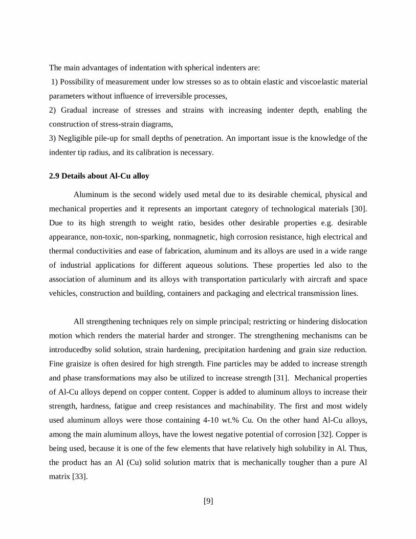
Figure 3 shows the Vickers microhardness, in HV, of the Al and Al-Cu alloys for the
compositions investigated in this study. Hardness is one of the most important properties, which
is commonly used to give a general indication of the strength and resistance to wear and
scratching of a material. It can be defined as the ability of a material to resist permanent
indentation or deformation when it is in contact with an indenter under load. In this study, the
initial microhardness of pure Al is 28 HV. The addition of Cu resulted in a linear increase of the
hardness of aluminum. The percentage improvements are 4, 25, and 46 % for 3, 6, and 9 wt. %
Cu contents, respectively. According to Man et. al [34], the hardness value of an Al-Mg-Si alloy
with 0.6% Cu is always distinctly higher than that of the alloy without Cu during isothermal
treatment.
Fig.2.5: shows with increasing cu content hardness of Al-Cu alloys increases
2.10.2 Grain size, impact energy, flow stress and mechanical characteristics
It can be noticed clearly that the addition of only 3 wt. % Cu resulted in grain refinement
of aluminum as the average grain size is decreased by 50 %, whereas addition of Cu at a rate of 6
wt. % and 9 wt. % resulted in grain refinement of aluminum by 69.2 % and 72.5 %, respectively.
However, there is a direct relationship between the copper content and the reduction in the grain
size diameter which it related to the enhancement of the mechanical characteristics of
commercially pure Al. Impact energy is a measure of the work done to fracture a test specimen.
It can be seen from the histogram that the addition of Cu to pure aluminum decreases the impact
[11]
energy by 22.4%, 33 % and 43% for 3 wt, % Cu, 6 wt. % Cu and 9 wt. % Cu, respectively.
Optimal impact energy is clearly noticed at 6 wt. % Cu. It can be seen from the histogram that
the addition of Cu to pure aluminum resulted in enhancement of the flow stress of pure
aluminum by 85.7 %, 73.2 %, and 101.8 % for 3 wt. % Cu, 6 wt. % Cu and 9 wt. % Cu,
respectively. Similar to the impact energy, an optimal value is clearly noticed at 6 wt. % Cu.
There is a direct relation between the copper addition and the mechanical characteristics
and the value is nearly similar for 3 wt. % Cu and 9 wt. % Cu additions, whereas it is different
and optimal for 6 wt. % Cu. This can be attributed to the fact that the maximum solubility of
copper in aluminum is about 5.65 %. According to Geng et. al[35], addition of Cu improved the
machinability of martensitic stainless steel 4Cr16Mo. The machinability of stainless steel was
optimal when the content of copper was 1.4%.
2.11 Application of Al-Cu alloys
Material competition in the automotive market has been traditionally intensive. Steel has
been the dominant material used in building automobiles since the 1920s. What types of
materials are likely to be winners in the 21st century? The automotive manufacturers’ decisions
on material’s usage are complex and are determined by a number of factors. The increasing
requirement to improve fuel economy triggered by concerns about global warming and energy
usage has a significant influence on the choice of materials. For example, the US government
regulations mandate that the automotive companies reduce vehicle exhaust emissions, improve
occupant safety, and enhance fuel economy [36]. To meet this requirement, automotive
manufacturers are making efforts to improve conventional engine efficiency, to develop new
power trains such as hybrid systems and to reduce vehicle weight.
Up to now the growth of aluminium in the automotive industry has been in the use of castings for
engine, transmission and wheel applications, and in heat exchangers. The cost of aluminium and
price stability remains its biggest impediment for its use in large-scale sheet applications.
Aluminium industry has targeted the automotive industry for future growth and has devote
significant resources to support this effort. The body-in-white (BIW) offers the greatest scope for
weight reduction with using large amount of aluminium. Recent developments have shown that
up to 50% weight saving for the BIW can be achieved by the substitution of steel by aluminium
[12]
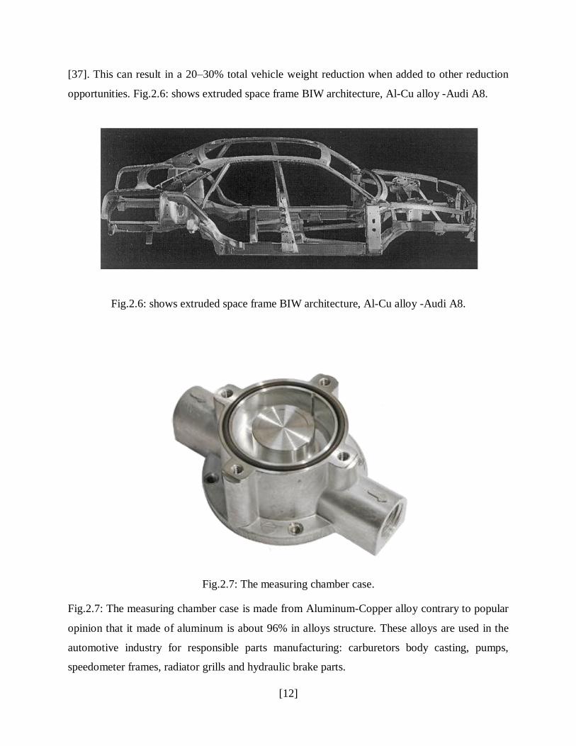
[37]. This can result in a 20–30% total vehicle weight reduction when added to other reduction
opportunities. Fig.2.6: shows extruded space frame BIW architecture, Al-Cu alloy -Audi A8.
Fig.2.6: shows extruded space frame BIW architecture, Al-Cu alloy -Audi A8.
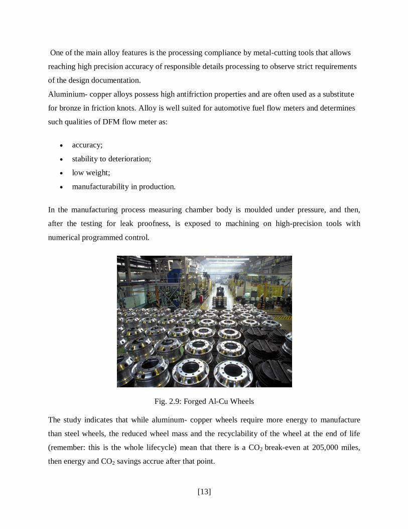
Fig.2.7: The measuring chamber case.
Fig.2.7: The measuring chamber case is made from Aluminum-Copper alloy contrary to popular
opinion that it made of aluminum is about 96% in alloys structure. These alloys are used in the
automotive industry for responsible parts manufacturing: carburetors body casting, pumps,
speedometer frames, radiator grills and hydraulic brake parts.
[13]
One of the main alloy features is the processing compliance by metal-cutting tools that allows
reaching high precision accuracy of responsible details processing to observe strict requirements
of the design documentation.
Aluminium- copper alloys possess high antifriction properties and are often used as a substitute
for bronze in friction knots. Alloy is well suited for automotive fuel flow meters and determines
such qualities of DFM flow meter as:
accuracy;
stability to deterioration;
low weight;
manufacturability in production.
In the manufacturing process measuring chamber body is moulded under pressure, and then,
after the testing for leak proofness, is exposed to machining on high-precision tools with
numerical programmed control.
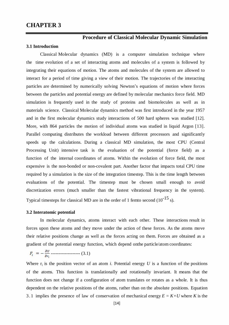
Fig. 2.9: Forged Al-Cu Wheels
The study indicates that while aluminum- copper wheels require more energy to manufacture
than steel wheels, the reduced wheel mass and the recyclability of the wheel at the end of life
(remember: this is the whole lifecycle) mean that there is a CO2 break-even at 205,000 miles,
then energy and CO2 savings accrue after that point.
CHAPTER 3
Procedure of Classical
Molecular Dynamic
Simulation
[14]
CHAPTER 3
Procedure of Classical Molecular Dynamic Simulation
3.1 Introduction
Classical Molecular dynamics (MD) is a computer simulation technique where
the time evolution of a set of interacting atoms and molecules of a system is followed by
integrating their equations of motion. The atoms and molecules of the system are allowed to
interact for a period of time giving a view of their motion. The trajectories of the interacting
particles are determined by numerically solving Newton’s equations of motion where forces
between the particles and potential energy are defined by molecular mechanics force field. MD
simulation is frequently used in the study of proteins and biomolecules as well as in
materials science. Classical Molecular dynamics method was first introduced in the year 1957
and in the first molecular dynamics study interactions of 500 hard spheres was studied [12].
More, with 864 particles the motion of individual atoms was studied in liquid Argon [13].
Parallel computing distributes the workload between different processors and significantly
speeds up the calculations. During a classical MD simulation, the most CPU (Central
Processing Unit) intensive task is the evaluation of the potential (force field) as a
function of the internal coordinates of atoms. Within the evolution of force field, the most
expensive is the non-bonded or non-covalent part. Another factor that impacts total CPU time
required by a simulation is the size of the integration timestep. This is the time length between
evaluations of the potential. The timestep must be chosen small enough to avoid
discretization errors (much smaller than the fastest vibrational frequency in the system).
Typical timesteps for classical MD are in the order of 1 femto second (10-15
s).
3.2 Interatomic potential
In molecular dynamics, atoms interact with each other. These interactions result in
forces upon these atoms and they move under the action of these forces. As the atoms move
their relative positions change as well as the forces acting on them. Forces are obtained as a
gradient of the potential energy function, which depend onthe particle/atom coordinates:
------------------- (3.1)
Where ri is the position vector of an atom i. Potential energy U is a function of the positions
of the atoms. This function is translationally and rotationally invariant. It means that the
function does not change if a configuration of atom translates or rotates as a whole. It is thus
dependent on the relative positions of the atoms, rather than on the absolute positions. Equation
3 . 1 implies the presence of law of conservation of mechanical energy E = K+U where K is the
[15]
kinetic energy.
3.3 Potentials in MD simulations
3.3.1 Embedded atom method (EAM)
Embedded atom method is an approximation describing the energy between two
atoms. The energy is a function of sum of functions of the separation between an atom and its
neighbors. It was first developed by Daw and Baskes (1984) for studying the defects in the
metals. EAMs are widely used in MD simulations. In the EAM (Daw and Baskes, 1984),
the total energy of an N- atom system is represented in the following equation [38]:-
------------------------- (3.2)
Where ( ) is a short range pair potential between atom i and j with the separation
distance , is the embedding energy of atom i with the electron density due to all its
neighbors is expressed below
------------------------- (3.3)
3.3.2 Empirical Potentials:
Those used in chemistry are frequently called force fields, while those used in
materials physics are called just empirical or analytical potentials. Most force fields in
chemistry are empirical and consist of a summation of bonded forces associated
with chemical bonds, bond angles, torsional forces and bond dihedrals and non-bonded forces
associated with vanderWaals forces and electrostatic charge. The total potential energy can be
expressed as:
Epot = ∑Vbond +∑ Vang +∑Vtorsion +∑VvdW +∑Vele + …---------------- (3.4)
Its calculation is the main culprit in the speed of MD simulations. Examples of such
potentials include the Brenner potential for hydrocarbons and its further developments for the
C-Si-H and C-O-H systems.
3.3.3 Pair wise Potentials & Many-Body Potentials:
In pair wise potentials, the total potential energy is calculated from the sum of energy
contributions between pairs of atoms. An example of such a pair potential is the non- bonded
Lennard–Jones potential used for calculating van der Waals forces.
[16]
In many-body potentials, the potential energy includes the effects of three or more
particles interacting w it h e a c h o t he r . In s i mu la t io ns w it h p a i r wise p o t e nt ia ls ,
g lo ba l interactions in the system also exist, but they occur only through pairwise terms. In
many- body potentials, the potential energy cannot be found by a sum over pairs of atoms, as
these interactions are calculated explicitly as a combination of higher-order terms. For
example, the Tersoff potential, which was originally used to simulate carbon, silicon and
germanium and the most widely used embedded-atom method (EAM).
3.3.4 Semi-Empirical Potentials:
It makes use of the matrix representation from quantum mechanics. The matrix is
then diagonalized to determine the occupancy of the different atomic orbitals, and empirical
formulae are used to determine the energy contributions of the orbitals.
3.3.5 Polarizable Potentials:
It includes the effect of polarizability, e.g. by measuring the partial charges obtained
from quantum chemical calculations. This allows for a dynamic redistribution of charge
between atoms which responds to the local chemical environment. For systems like water and
protein better simulation results obtained by introducing polarizability.
3.4 Ab-initio Quantum-Mechanical Methods:
Ab-initio calculations produce a vast amount of information that is not available from
empirical methods, such as density of electronic states or other electronic properties. A
significant advantage of using ab-initio methods is the ability to study reactions that
involve breaking or formation of covalent bonds, which correspond to multiple electronic
states.Another parameter that affects total CPU time required by a simulation is the size of the
integration timestep. This is the time length between evaluations of the potential function. The
time step must be chosen small enough to avoid discretization errors (i.e. smaller than the
fastest vibrational frequency in the system). Typical time steps for classical MD are in the order
of 1 femtosecond (10−15
s). Proper time integration algorithm should be implemented to
achieve optimum simulation time.Time integration algorithms are based on finite difference
methods, where time is discretized on a finite grid, the time step being the distance between
consecutive points on the grid. Knowing the positions and some of their time derivatives at
time t, the integration scheme gives the same quantities at a later time t+ . By iterating the
[17]
procedure, the time evolution of the system can be followed for long times. The schemes are
approximate and there are errors associated with them which can be reduced by decreasing .
Two popular integration methods for MD calculations are the Verlet algorithm and Predictor-
corrector algorithms. The most widely used time integration algorithm is the Verlet algorithm. In
this case, the position of a particle at any time t is given by:
V (t) = {r(t+Δt) – r(t-Δt)}/2Δt.....................................------------(3.5)
Where V (t) = Velocity of a particle at time t.
r (t) = position of a particle at time t.
Δt = Small change in time.
The predictor-corrector algorithm consists of three steps
Step 1: Predictor: From the positions and their time derivatives at time t, one ‘predicts’
the same quantities at time t+ by means of a Taylor expansion. One such quantity is
acceleration.
Step 2: Force evaluation: The force is computed by taking the gradient of the potential at the
predicted positions. The difference between the resulting acceleration and the predicted
acceleration gives error.
Step 3: Corrector. This error signal is used to ‘correct’ positions and their derivatives.All the
corrections are proportional to the error signal, the coefficient of proportionality
being determined to maximize the stability of the algorithm.
In all kinds of molecular dynamics simulations, the simulation box size must be large
enough to avoid surface effects. Atoms near the boundary have fewer neighbours than atoms
inside resulting surface effects in the simulation to be much more important than they are in the
real system. Boundary conditions are often treated by choosing fixed values at the edges (which
may cause surface effects), or by employing periodic boundary conditions where the particles
interact across the boundary and can move from one end to another end.
3.5 Simulation method in Molecular dynamics
MD simulation is a technique for computing the equilibrium and transport
properties of a classical many-body system. In classical MD the molecular motion obeys
the laws of classical mechanics. Given an initial set of position and velocities of atoms
(phase space), the subsequent time evolution is determined. The result is a trajectory
[18]
that specifies how the position and velocities of the atoms in the system vary with time.
The trajectory is obtained by solving the differential equations embodied in Newton’s
second law (Force = mass × acceleration)
----------------------------------- (3.6)
This equation describes the motion of particle of mass mi along one coordinate
(xi) with Fxi being the net force on the particle in that direction.
3.6 General steps of molecular dynamics simulation
i. Assigning the initial positions and velocities of the atoms
ii. Computing the forces on all the atoms based on interatomic potential Integrating Newton’s
equation of motion for obtaining the trajectory.
iii. The above and the present step make up the core of the simulation. They are repeated until
time evolution of the desired property of the system is obtained.
3.7 Periodic boundary condition
Periodic boundary condition is used to simulate a large system by modeling a small
part (primary cell) that is far from its edge. The primary cell chosen has no surface effect.
3.8 Ensembles
(a) Micro-canonical or NVE
In the micro-canonical NVE ensemble the system is isolated from changes in atoms
(N), volume (V) and energy (E). NVE integrator updates position and velocity for atoms
in the group each timestep. It corresponds to an adiabatic process with no heat exchange. The
trajectory of atoms in the system is generated during which there is an exchange of potential
and kinetic energy, and the total energy is conserved.
(b) Canonical or NVT
In the canonical ensemble NVT, the number of atoms (N), volume of the system (V) and the
system temperature (T) are the independent variables and are kept constant. Temperature is
controlled by Noose-Hover thermostat.
(c) Isothermal–Isobaric or NPT
NPT is the isothermal-isobaric ensemble in which number of atoms (N), pressure (P)
and temperature (T) are conserved. The volume of the system is allowed to change over
time. Temperature and pressure are controlled by Nose-Hoover thermostat and Nose
Hoover barostat.
3.9 Calculation of Temperature
The relation between kinetic energy and temperature is given below
[19]
--------------------- (3.7)
k = Boltzmann constant
N = number of particles/atoms
m = particle mass
v = root-mean square velocity
3.10 Introduction to LAMMPS (Large-scale Atomic/Molecular Massively Parallel
Simulator)
3.10.1 Background
LAMMPS is a classical molecular dynamics code (Plimpton, 1995). It was
developed at Sandia National Laboratories, which is under United States Department of
Energy. It is distributed as an open source code under general public license
(http://lammps.sandia.gov). The features of LAMMPS are briefly described in the following
section.
3.10.2 General features
The general features of LAMMPS are as follows:
i. runs on single processor or parallel processors
ii. distributed-memory message-passing parallelism (MPI)
iii. spatial-decomposition of simulation domain for parallelism
iv. optional libraries used: MPI and single-processor FFT
v. runs from an input script
vi. syntax for defining and using variables and formulas
vii. syntax for looping over runs and breaking out of loops
3.10.3 Force fields
Some of the force fields that are employed in LAMMPS are:
i. pairwise potentials: Lennard-Jones, Buckhingam, Morse, Born-Mayer-
Huggins, Yukawa, soft, class 2 (COMPASS), hydrogen bond.
ii. charged pairwise potentials: Coulombic, point-dipole
iii. manybody potentials: EAM, Finnis/Sinclair EAM,modified EAM
3.10.4 Atoms creation
[20]
The various methods of creating atoms are:
i. read_data – this command reads the initial atom coordinates from an
ASCII text or a gzipped text file.
ii. lattice – this command creates atoms, in the lattice points inside the
simulation box.
iii. delete_atoms – this can be used to deletes atoms in order to create void.
iv. displace_atoms – this can be used to move atoms a large distance before
beginning a simulation or to randomize atoms initially on a lattice
3.10.5 Ensembles, constraints, and boundary conditions
In LAMMPS ‘fix’ is any operation that is applied to the system during time
stepping or minimization. For example, the updating of atom positions and velocities due to
time integration, controlling temperature, applying constraint forces to atoms, enforcing
boundary conditions, and computing diagnostics etc. Fixes perform their operations at
different stages of the timestep. If two or more fixes operate at the same stage of the
timestep, they are invoked in the order they were specified in the input script.
3.10.6 Boundary conditions
The boundary conditions that are employed in LAMMPS are:
i. p p p
ii. p p s
iii. p f p
Where ‘p’ stands for periodic along the three directions, ‘f’ and‘s’ stand for fixed and
shrink wrapped, which are non-periodic.
3.10.7 Integrator
The integrators that are available in LAMMPS are:
i. velocity-Verlet integrator
ii. Brownian dynamics
iii. rigid body integration
iv. energy minimization via conjugate or steepest descent relaxation
3.10.8 Energy minimization

[21]
LAMMPS performs an energy minimization of the system, by iteratively adjusting
atom coordinates. Iterations are terminated when one of the stopping criteria is satisfied. At
that point the system will be in local minimum potential energy. The minimization
algorithm used is set by the ‘min_style’ command. The minimizers bound the distance
atoms movement in single iteration, so that it is possible to relax systems with highly
overlapped atoms (large energies and forces) by pushing the atoms off each other.
3.10.9 LAMMPS input script
LAMMPS executes by reading commands from an input script (text file), one line at a
time. When the input script ends, LAMMPS exits. Each command causes LAMMPS to take
some action. It may set an internal variable, read in a file, or run a simulation. Most
commands have default settings, which can be changed upon once requirements. LAMMPS
input script typically consists of four parts:
i. Initialization
ii. atom definition
iii. Settings
iv. run a Simulation
i. Initialization commands used in the present study
units metal
boundary p p p
atom_style atomic
pair_style eam/alloy
read_data indent.txt
ii. Atom definition commands used in the present study
region box block 0 100 0 100 0 100 units box
create_box 2 box
lattice fcc 4.05
iii. Settings used in the present study
The next step after defining atoms is settting up force field coefficients, simulation
parameters, output options etc.
pair_coeff * * A l C u . e a m . a l l o y A l C u (force field parameter)
minimize 1.0e-3 1.0e-6 10000 10000 (energy minimization)
timestep 0.002
[22]
thermo 100 (output)
dump 1 all atom 10 7030n_cryst_3d_large.lammpstrj (output)
log log7030n_cryst_3d_large.data
iv. Run a simulation
MD simulation is run using the ‘run’ command.
3.11 Output
After successful running of the in.file, we will get four out-put files as follows:
a) DUMP file (containing the atomic co-ordinates of the final structure after simulation
and also for deformation studies it contains the stress Component values).
b) RDF file (contains co-ordination values of atoms and radial distribution function
values). RDF or radial distribut ion funct ion is a measure of arrangement of atoms
in the material.
c) Log file (contains thermodynamic data e.g temperature, pressure, volume, and total
energy after a particular no of steps).
d) Log. lammps file
The output of the LAMMPS simulation is written onto text files called dump file
containing the information of the atom coordinates along with the velocities dumped at the
required time step. They also contain per-atom quantities. While the thermodynamic
information of the simulation is stored as log file.
3.12 Simulation studies performed using LAMMPS
3.12.1Nano-indentation deformation study
The command used for nano-indentation in the present study is ‘indent’. The indenter
used is spherical indenter.
fix 4 m o b i l e i n d e n t 1 0 0 0 . 0 s p h e r e 5 0 v _ y 5 0 1 5 . 0 u n i t s b o x
3.13 Visual Molecular dynamics (VMD)
VMD is a molecular graphics program designed for the display and analysis of molecular
assemblies, in particular biopolymers such as proteins and nucleic acids. VMD can
simultaneously display any number of structures using a wide variety of rendering styles and
coloring methods. Molecules are displayed as one or more "representations," in which each
representation embodies a particular rendering method and coloring scheme for a selected subset
of atoms. The atoms displayed in each representation are chosen using an extensive atom
selection syntax, which includes Boolean operators and regular expressions. VMD is a
molecular visualization package for displaying, animating, and analyzing large
atoms/molecules using 3-D graphics and built-in scripting. In the present study all the atomic
snapshots are taken by VMD software [40].

CHAPTER 4
Results &
Discussion
[23]
CHAPTER 4
RESULT AND DISSCUSSION
4. Results and Discussion
In this work we carried out molecular dynamics simulation deformation studies of
Al-Cu alloys (Al70-Cu30, Al67-Cu33 and Al50-Cu50) by nano-indentaion. The effect of
composition, strain rate, temperature and indenter diameter were investigated. The
following paragraphs describe the methods of creation of crystalline alloys and their
analysis by radial distribution function (RDF) followed by indentation studies of the alloys.
4.1 Creation of Al-Cu Crystalline alloy
Crystall ine model was created by Isothermal-Isobaric canonical ensemble using the
LAMMPS code performing 2000 integration steps at 300K and timestep of 0.002 ps (pico
seconds) with box size (100Å×100Å×100Å) consisting of 62500 atoms. Three crystalline
models were created i.e Al70-Cu30, Al67-Cu33, Al50-Cu50 alloys having the same box size.
VMD snap shots, RDF and time vs. temperature plots of all the alloys are given below.
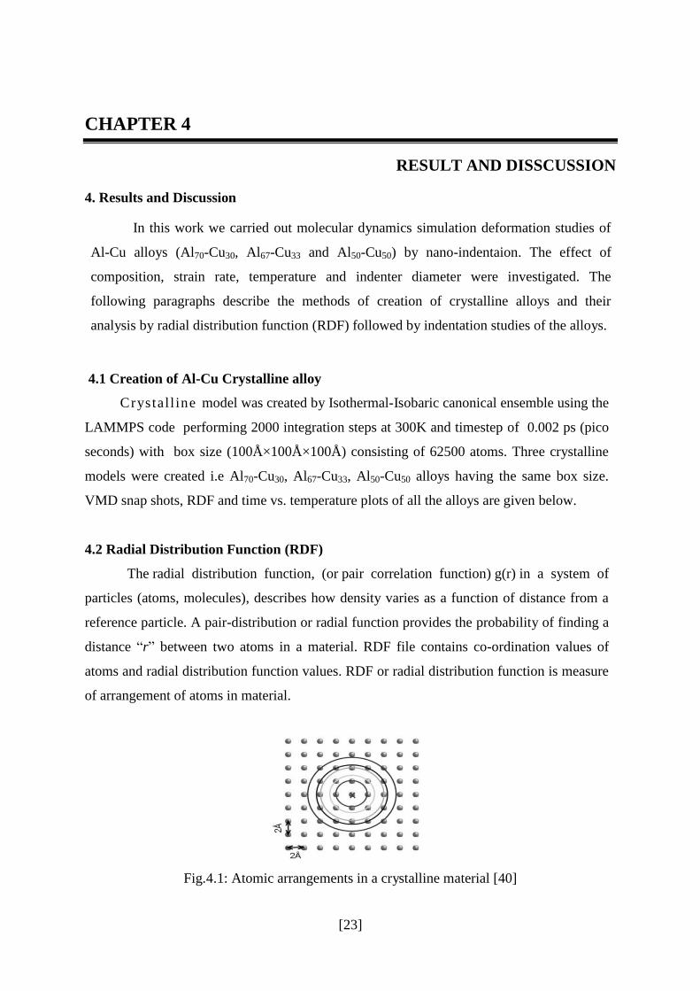
4.2 Radial Distribution Function (RDF)
The radial distribution function, (or pair correlation function) g(r) in a system of
particles (atoms, molecules), describes how density varies as a function of distance from a
reference particle. A pair-distribution or radial function provides the probability of finding a
distance “r” between two atoms in a material. RDF file contains co-ordination values of
atoms and radial distribution function values. RDF or radial distribution function is measure
of arrangement of atoms in material.
Fig.4.1: Atomic arrangements in a crystalline material [40]
[24]
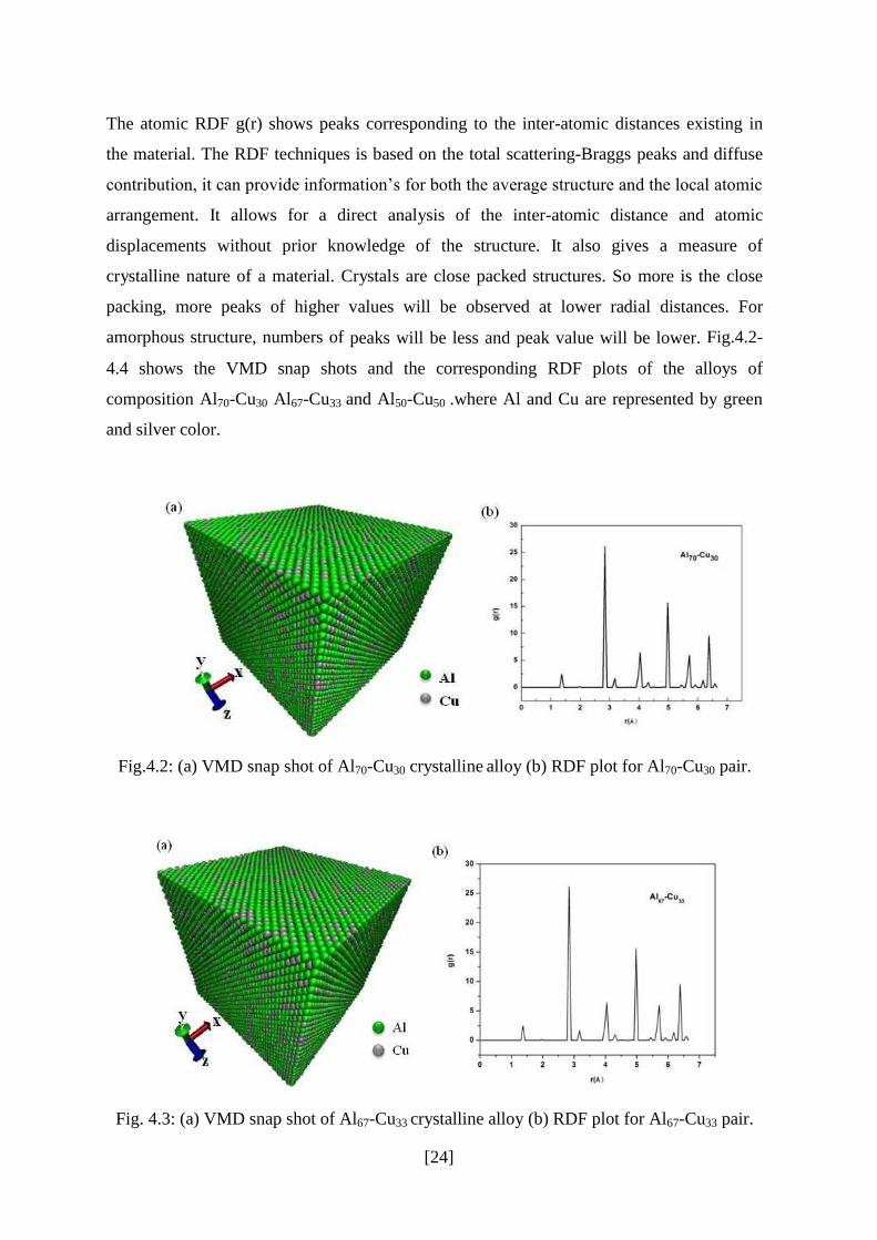
The atomic RDF g(r) shows peaks corresponding to the inter-atomic distances existing in
the material. The RDF techniques is based on the total scattering-Braggs peaks and diffuse
contribution, it can provide information’s for both the average structure and the local atomic
arrangement. It allows for a direct analysis of the inter-atomic distance and atomic
displacements without prior knowledge of the structure. It also gives a measure of
crystalline nature of a material. Crystals are close packed structures. So more is the close
packing, more peaks of higher values will be observed at lower radial distances. For
amorphous structure, numbers of peaks will be less and peak value will be lower. Fig.4.2-
4.4 shows the VMD snap shots and the corresponding RDF plots of the alloys of
composition Al70-Cu30 Al67-Cu33 and Al50-Cu50 .where Al and Cu are represented by green
and silver color.
Fig.4.2: (a) VMD snap shot of Al70-Cu30 crystalline alloy (b) RDF plot for Al70-Cu30 pair.
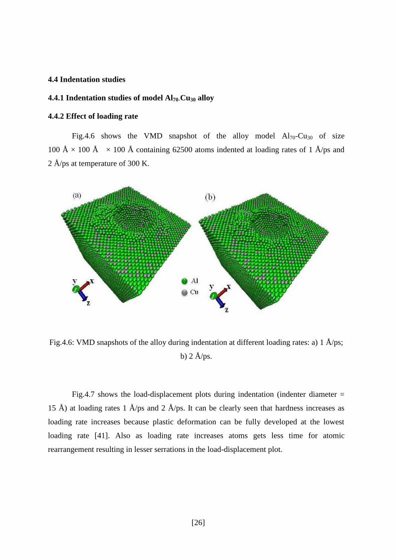
Fig. 4.3: (a) VMD snap shot of Al67-Cu33 crystalline alloy (b) RDF plot for Al67-Cu33 pair.

[25]
Fig.4.4: (a) VMD snap shot of Al50-Cu50 crystalline alloy (b) RDF plot for Al50-Cu50 pair.
4.3 Time step vs. Temperature plots
It shows the average of the instantaneous kinetic temperature over many molecular
dynamic time steps. Fig.4.5 shows the Time step vs. Temperature plots for (a) Al70-Cu30 (b)
Al67-Cu33 and (c) Al50-Cu50alloy. From the temperature-time plots it is clear that the
structures are stabilized at room temperature.
Fig.4.5: Time step vs. Temperature plot for (a) Al70-Cu30 (b) Al67-Cu33 and (c) Al50-Cu50
alloy.
[26]
4.4 Indentation studies
4.4.1 Indentation studies of model Al70-Cu30 alloy
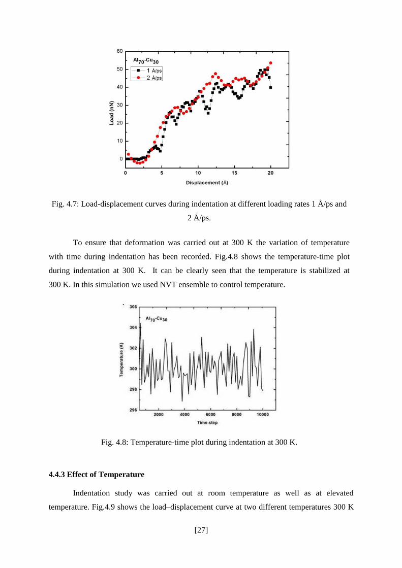
4.4.2 Effect of loading rate
Fig.4.6 shows the VMD snapshot of the alloy model Al70-Cu30 of size
100 Å × 100 Å × 100 Å containing 62500 atoms indented at loading rates of 1 Å/ps and
2 Å/ps at temperature of 300 K.
Fig.4.6: VMD snapshots of the alloy during indentation at different loading rates: a) 1 Å/ps;
b) 2 Å/ps.
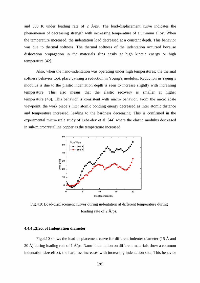
Fig.4.7 shows the load-displacement plots during indentation (indenter diameter =
15 Å) at loading rates 1 Å/ps and 2 Å/ps. It can be clearly seen that hardness increases as
loading rate increases because plastic deformation can be fully developed at the lowest
loading rate [41]. Also as loading rate increases atoms gets less time for atomic
rearrangement resulting in lesser serrations in the load-displacement plot.
[27]
Fig. 4.7: Load-displacement curves during indentation at different loading rates 1 Å/ps and
2 Å/ps.
To ensure that deformation was carried out at 300 K the variation of temperature
with time during indentation has been recorded. Fig.4.8 shows the temperature-time plot
during indentation at 300 K. It can be clearly seen that the temperature is stabilized at
300 K. In this simulation we used NVT ensemble to control temperature.
Fig. 4.8: Temperature-time plot during indentation at 300 K.
4.4.3 Effect of Temperature
Indentation study was carried out at room temperature as well as at elevated
temperature. Fig.4.9 shows the load–displacement curve at two different temperatures 300 K
[28]
and 500 K under loading rate of 2 Å/ps. The load-displacement curve indicates the
phenomenon of decreasing strength with increasing temperature of aluminum alloy. When
the temperature increased, the indentation load decreased at a constant depth. This behavior
was due to thermal softness. The thermal softness of the indentation occurred because
dislocation propagation in the materials slips easily at high kinetic energy or high
temperature [42].
Also, when the nano-indentation was operating under high temperatures; the thermal
softness behavior took place causing a reduction in Young’s modulus. Reduction in Young’s
modulus is due to the plastic indentation depth is seen to increase slightly with increasing
temperature. This also means that the elastic recovery is smaller at higher
temperature [43]. This behavior is consistent with macro behavior. From the micro scale
viewpoint, the work piece’s inter atomic bonding energy decreased as inter atomic distance
and temperature increased, leading to the hardness decreasing. This is confirmed in the
experimental micro-scale study of Lebe-dev et al. [44] where the elastic modulus decreased
in sub-microcrystalline copper as the temperature increased.
Fig.4.9: Load-displacement curves during indentation at different temperature during
loading rate of 2 Å/ps.
4.4.4 Effect of Indentation diameter
Fig.4.10 shows the load-displacement curve for different indenter diameter (15 Å and
20 Å) during loading rate of 1 Å/ps. Nano- indentation on different materials show a common
indentation size effect, the hardness increases with increasing indentation size. This behavior
[29]
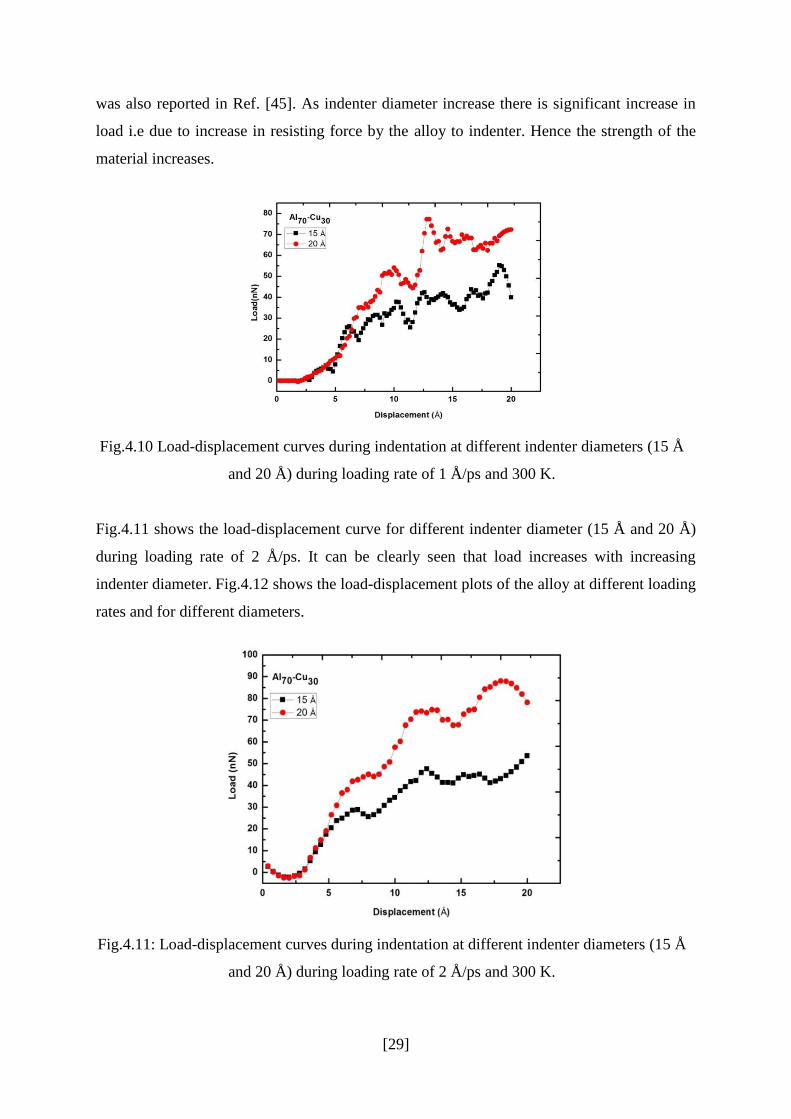
was also reported in Ref. [45]. As indenter diameter increase there is significant increase in
load i.e due to increase in resisting force by the alloy to indenter. Hence the strength of the
material increases.
Fig.4.10 Load-displacement curves during indentation at different indenter diameters (15 Å
and 20 Å) during loading rate of 1 Å/ps and 300 K.
Fig.4.11 shows the load-displacement curve for different indenter diameter (15 Å and 20 Å)
during loading rate of 2 Å/ps. It can be clearly seen that load increases with increasing
indenter diameter. Fig.4.12 shows the load-displacement plots of the alloy at different loading
rates and for different diameters.
Fig.4.11: Load-displacement curves during indentation at different indenter diameters (15 Å
and 20 Å) during loading rate of 2 Å/ps and 300 K.
[30]
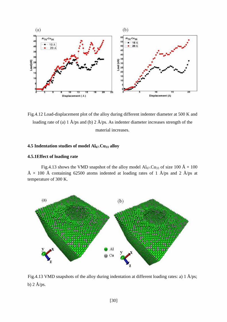
Fig.4.12 Load-displacement plot of the alloy during different indenter diameter at 500 K and
loading rate of (a) 1 Å/ps and (b) 2 Å/ps. As indenter diameter increases strength of the
material increases.
4.5 Indentation studies of model Al67-Cu33 alloy
4.5.1Effect of loading rate
Fig.4.13 shows the VMD snapshot of the alloy model Al67-Cu33 of size 100 Å × 100
Å × 100 Å containing 62500 atoms indented at loading rates of 1 Å/ps and 2 Å/ps at
temperature of 300 K.
Fig.4.13 VMD snapshots of the alloy during indentation at different loading rates: a) 1 Å/ps;
b) 2 Å/ps.
[31]
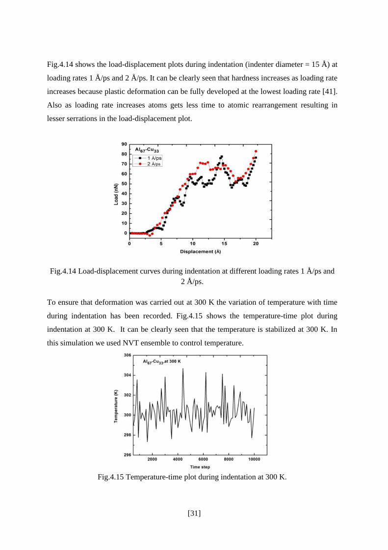
Fig.4.14 shows the load-displacement plots during indentation (indenter diameter = 15 Å) at
loading rates 1 Å/ps and 2 Å/ps. It can be clearly seen that hardness increases as loading rate
increases because plastic deformation can be fully developed at the lowest loading rate [41].
Also as loading rate increases atoms gets less time to atomic rearrangement resulting in
lesser serrations in the load-displacement plot.
Fig.4.14 Load-displacement curves during indentation at different loading rates 1 Å/ps and
2 Å/ps.
To ensure that deformation was carried out at 300 K the variation of temperature with time
during indentation has been recorded. Fig.4.15 shows the temperature-time plot during
indentation at 300 K. It can be clearly seen that the temperature is stabilized at 300 K. In
this simulation we used NVT ensemble to control temperature.
Fig.4.15 Temperature-time plot during indentation at 300 K.
[32]
4.5.2 Effect of Temperature
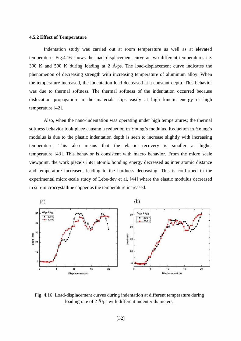
Indentation study was carried out at room temperature as well as at elevated
temperature. Fig.4.16 shows the load–displacement curve at two different temperatures i.e.
300 K and 500 K during loading at 2 Å/ps. The load-displacement curve indicates the
phenomenon of decreasing strength with increasing temperature of aluminum alloy. When
the temperature increased, the indentation load decreased at a constant depth. This behavior
was due to thermal softness. The thermal softness of the indentation occurred because
dislocation propagation in the materials slips easily at high kinetic energy or high
temperature [42].
Also, when the nano-indentation was operating under high temperatures; the thermal
softness behavior took place causing a reduction in Young’s modulus. Reduction in Young’s
modulus is due to the plastic indentation depth is seen to increase slightly with increasing
temperature. This also means that the elastic recovery is smaller at higher
temperature [43]. This behavior is consistent with macro behavior. From the micro scale
viewpoint, the work piece’s inter atomic bonding energy decreased as inter atomic distance
and temperature increased, leading to the hardness decreasing. This is confirmed in the
experimental micro-scale study of Lebe-dev et al. [44] where the elastic modulus decreased
in sub-microcrystalline copper as the temperature increased.
Fig. 4.16: Load-displacement curves during indentation at different temperature during
loading rate of 2 Å/ps with different indenter diameters.
[33]
4.5.3 Effect of Indentation diameter
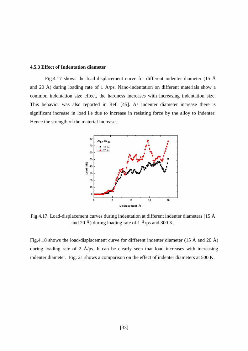
Fig.4.17 shows the load-displacement curve for different indenter diameter (15 Å
and 20 Å) during loading rate of 1 Å/ps. Nano-indentation on different materials show a
common indentation size effect, the hardness increases with increasing indentation size.
This behavior was also reported in Ref. [45]. As indenter diameter increase there is
significant increase in load i.e due to increase in resisting force by the alloy to indenter.
Hence the strength of the material increases.
Fig.4.17: Load-displacement curves during indentation at different indenter diameters (15 Å
and 20 Å) during loading rate of 1 Å/ps and 300 K.
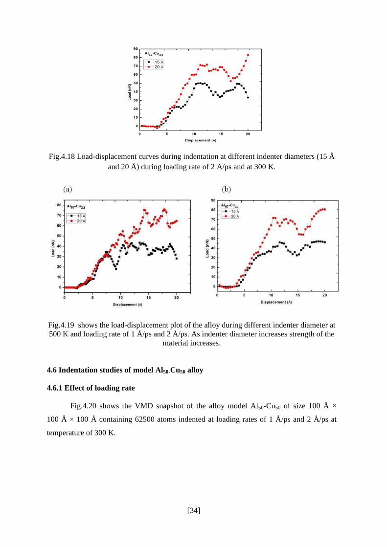
Fig.4.18 shows the load-displacement curve for different indenter diameter (15 Å and 20 Å)
during loading rate of 2 Å/ps. It can be clearly seen that load increases with increasing
indenter diameter. Fig. 21 shows a comparison on the effect of indenter diameters at 500 K.
[34]
Fig.4.18 Load-displacement curves during indentation at different indenter diameters (15 Å
and 20 Å) during loading rate of 2 Å/ps and at 300 K.
Fig.4.19 shows the load-displacement plot of the alloy during different indenter diameter at
500 K and loading rate of 1 Å/ps and 2 Å/ps. As indenter diameter increases strength of the
material increases.
4.6 Indentation studies of model Al50-Cu50 alloy
4.6.1 Effect of loading rate
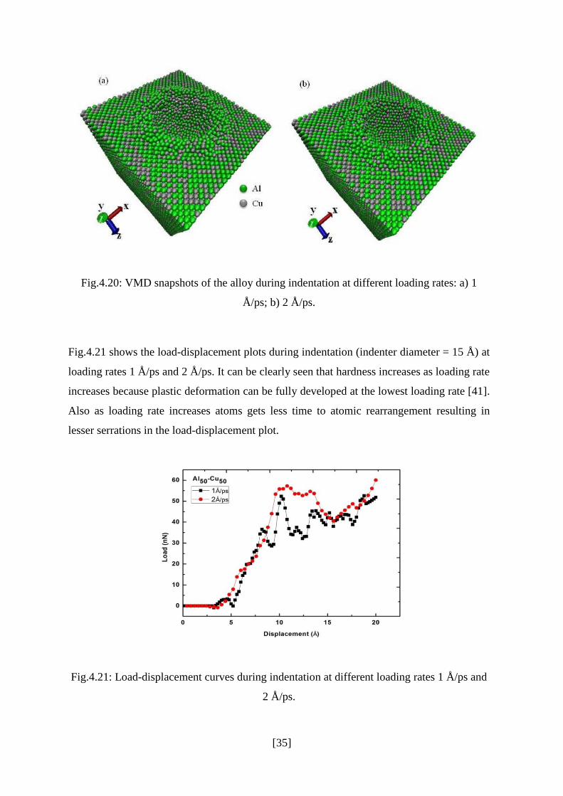
Fig.4.20 shows the VMD snapshot of the alloy model Al50-Cu50 of size 100 Å ×
100 Å × 100 Å containing 62500 atoms indented at loading rates of 1 Å/ps and 2 Å/ps at
temperature of 300 K.
[35]
Fig.4.20: VMD snapshots of the alloy during indentation at different loading rates: a) 1
Å/ps; b) 2 Å/ps.
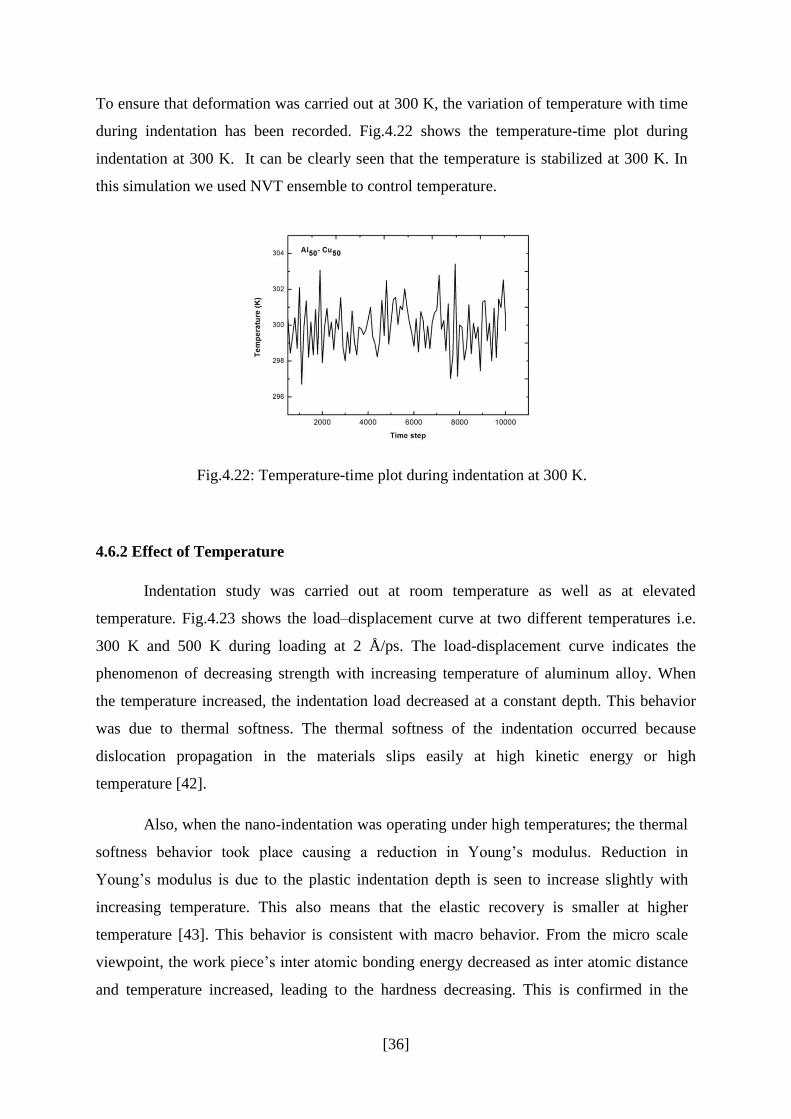
Fig.4.21 shows the load-displacement plots during indentation (indenter diameter = 15 Å) at
loading rates 1 Å/ps and 2 Å/ps. It can be clearly seen that hardness increases as loading rate
increases because plastic deformation can be fully developed at the lowest loading rate [41].
Also as loading rate increases atoms gets less time to atomic rearrangement resulting in
lesser serrations in the load-displacement plot.
Fig.4.21: Load-displacement curves during indentation at different loading rates 1 Å/ps and
2 Å/ps.
[36]
To ensure that deformation was carried out at 300 K, the variation of temperature with time
during indentation has been recorded. Fig.4.22 shows the temperature-time plot during
indentation at 300 K. It can be clearly seen that the temperature is stabilized at 300 K. In
this simulation we used NVT ensemble to control temperature.
Fig.4.22: Temperature-time plot during indentation at 300 K.
4.6.2 Effect of Temperature
Indentation study was carried out at room temperature as well as at elevated
temperature. Fig.4.23 shows the load–displacement curve at two different temperatures i.e.
300 K and 500 K during loading at 2 Å/ps. The load-displacement curve indicates the
phenomenon of decreasing strength with increasing temperature of aluminum alloy. When
the temperature increased, the indentation load decreased at a constant depth. This behavior
was due to thermal softness. The thermal softness of the indentation occurred because
dislocation propagation in the materials slips easily at high kinetic energy or high
temperature [42].
Also, when the nano-indentation was operating under high temperatures; the thermal
softness behavior took place causing a reduction in Young’s modulus. Reduction in
Young’s modulus is due to the plastic indentation depth is seen to increase slightly with
increasing temperature. This also means that the elastic recovery is smaller at higher
temperature [43]. This behavior is consistent with macro behavior. From the micro scale
viewpoint, the work piece’s inter atomic bonding energy decreased as inter atomic distance
and temperature increased, leading to the hardness decreasing. This is confirmed in the
[37]
experimental micro-scale study of Lebe-dev et al. [44]. Where the elastic modulus decreased
in sub-microcrystalline copper as the temperature increased.
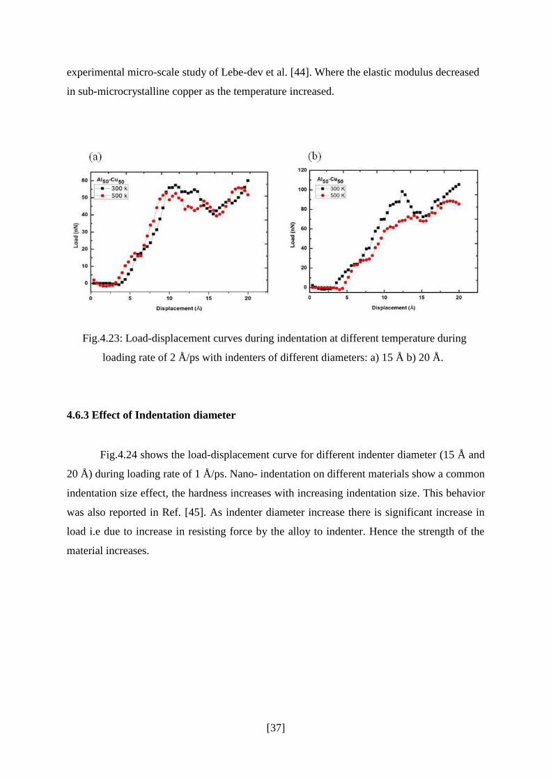
Fig.4.23: Load-displacement curves during indentation at different temperature during
loading rate of 2 Å/ps with indenters of different diameters: a) 15 Å b) 20 Å.
4.6.3 Effect of Indentation diameter
Fig.4.24 shows the load-displacement curve for different indenter diameter (15 Å and
20 Å) during loading rate of 1 Å/ps. Nano- indentation on different materials show a common
indentation size effect, the hardness increases with increasing indentation size. This behavior
was also reported in Ref. [45]. As indenter diameter increase there is significant increase in
load i.e due to increase in resisting force by the alloy to indenter. Hence the strength of the
material increases.
[38]
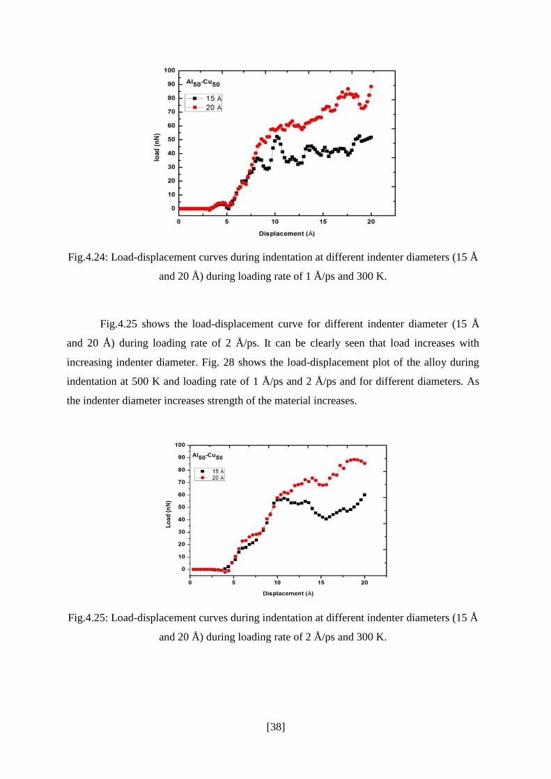
Fig.4.24: Load-displacement curves during indentation at different indenter diameters (15 Å
and 20 Å) during loading rate of 1 Å/ps and 300 K.
Fig.4.25 shows the load-displacement curve for different indenter diameter (15 Å
and 20 Å) during loading rate of 2 Å/ps. It can be clearly seen that load increases with
increasing indenter diameter. Fig. 28 shows the load-displacement plot of the alloy during
indentation at 500 K and loading rate of 1 Å/ps and 2 Å/ps and for different diameters. As
the indenter diameter increases strength of the material increases.
Fig.4.25: Load-displacement curves during indentation at different indenter diameters (15 Å
and 20 Å) during loading rate of 2 Å/ps and 300 K.
[39]
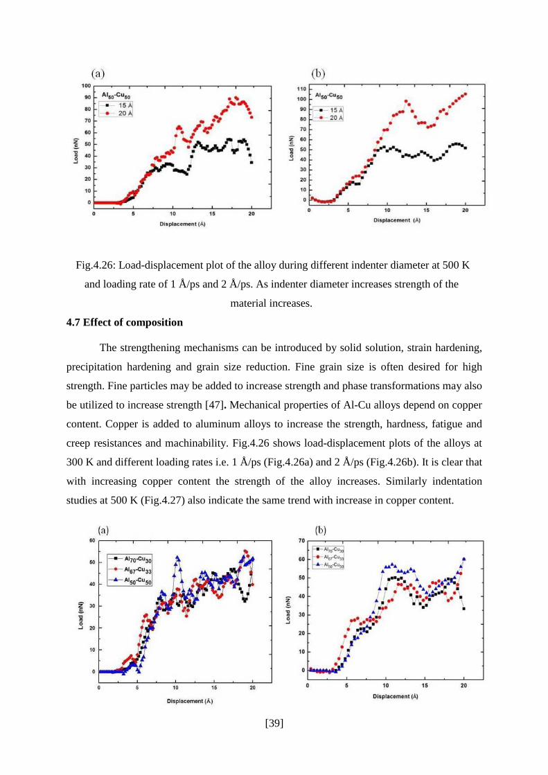
Fig.4.26: Load-displacement plot of the alloy during different indenter diameter at 500 K
and loading rate of 1 Å/ps and 2 Å/ps. As indenter diameter increases strength of the
material increases.
4.7 Effect of composition
The strengthening mechanisms can be introduced by solid solution, strain hardening,
precipitation hardening and grain size reduction. Fine grain size is often desired for high
strength. Fine particles may be added to increase strength and phase transformations may also
be utilized to increase strength [47]. Mechanical properties of Al-Cu alloys depend on copper
content. Copper is added to aluminum alloys to increase the strength, hardness, fatigue and
creep resistances and machinability. Fig.4.26 shows load-displacement plots of the alloys at
300 K and different loading rates i.e. 1 Å/ps (Fig.4.26a) and 2 Å/ps (Fig.4.26b). It is clear that
with increasing copper content the strength of the alloy increases. Similarly indentation
studies at 500 K (Fig.4.27) also indicate the same trend with increase in copper content.
[40]
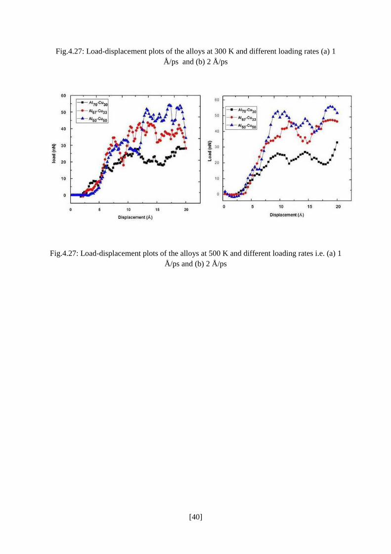
Fig.4.27: Load-displacement plots of the alloys at 300 K and different loading rates (a) 1
Å/ps and (b) 2 Å/ps
Fig.4.27: Load-displacement plots of the alloys at 500 K and different loading rates i.e. (a) 1
Å/ps and (b) 2 Å/ps

CHAPTER 5 Conclusion
[40]
CHAPTER 5
CONCLUSION
5. Conclusion and Scope for future work
5.1 Conclusion
a) In summary, in order to better understand the nan-oindentation deformation
mechanism, MD simulation was performed at different indenter diameter, loading
rates and temperatures for Al-Cu alloys during nano-indentation.
b) MD simulation reveals that with increase in loading rate atoms gets less time to
atomic rearrangement resulting in lesser serrations in the load-displacement plot.
Further hardness increases as loading rate increases because plastic deformation can
be fully developed at the lowest loading rate.
c) As indenter diameter increase there is significant increase in load i.e due to increase in
resisting force by the alloy to indenter. Hence the strength of the material increases.
d) In addition, the results also indicated that the indentation rates which are the main
reason for the deformation mechanism and during indentation caused thermal softens
to occur. The simulation results indicated that hardness became lower as the
temperature increase.
e) MD simulation nano-indentation results indicate that with increase in Cu content
hardness of the Al-Cu alloys increases. Mechanical properties of Al-Cu alloys depend
on copper content. Copper is added to aluminium alloys to increase the strength,
hardness, fatigue and creep resistances and machinability.
5.2 Scope for Future Work
a) Simulation studies are to be carried out to understand the structure of crystalline alloy
and their evolution during deformation.
b) A large-scale simulation study on self-assembly of nano-scale heterogeneity is
required.
c) Simulation studies on loading-unloading of the crystalline structure to exactly
determine the strength.

CHAPTER 6
References
CHAPTER 6
REFERENCES
Reference
1. Rahman, A. (1964), Correlations in the Motion of Atoms in Liquid Argon, Physical
Review, Vol. 136, No. 2A, pp. A405-A411
2. Polmear, I.J. (1980) Light Alloys, vol.45 No.12 pp.3256-3263
3. Yakibchuk.P , Patsahan.v, Patsahan.T ; Molecular dynamics simulation of Al-Cu alloys.
Rollasaon, R. (1973). Metallurgy for engineers, 4th
Edition, Edward Arnold, Great
Britain.
4. Rooy, E.L. (1988). Metals Handbook, 15, ASM International, Materials Park, Ohio, 743.
5. Aravind, M., Yu, P., Yau, M.Y. and Ng, D.H.L. (2004). Formation of Al2Cu and AlCu
6. intermetallics in Al(Cu) alloy matrix composites by reaction sintering. Materials Science
and Engineering A380 pp.384-393.
7. B.Halliop,M.F.Salaun, (2012)vol.358 issue 17,pp 2227-2231.
8. Shechtman, D. , Blech,I., D. Gratias, and J. W. Cahn, (1984). Phys. Rev. Lett. 53, 1951
9. N. W. Ashcroft and N. D. Mermin, (1985) Solid State Physics (Saunders College
Publishing, Texas).
10. Alder ,B.J. and Wainwright, T.E.J. (1957) Chem. Phys. 27.1208
11. Alder ,B.J. and Wainwright, T.E.J. (1959) Chem. Phys. 27.1208.
12. Rahman , A.Phys.Rev. (1964) A136, 405.
13. Stillinger, F.H. and Rahaman, (1974) A.J.Chem.Phys.60, 1545
14. McCommon, J.A,Gelin,B.R, and Karplus,M.Nature(lond(1977)) 267,585.
15. Rapaport, D C, (1995) “The Art of Molecular Dynamics Simulation”, Cambridge
University Press, J. B. Pethica, R. Hutchings and W. C. Oliver, (1983) Phil. Mag. A 48,
593.
16. M. F. Doerner and W. D. Nix, (1986) J. Mater. Res. 1, 601.
17. W. C. Oliver, and G. M. Pharr, (1992) J. Mater. Res. 7, 1564.
18. H. A. Francis, (1976) J. Eng. Mater. Tech. 98, 272.
19. Oliver W.C., Pharr G.M.; (1992) J. Mater. Res., vol.7, No.6, pp.1564-1583.
20. jaroslav mencik , (2011) Chem. Listy 105, s680-s683.
21. Robertson J.: (2002) Mater. Sci Eng. R. 37, 129.
22. Venkatesh T.A., et.al.; ( 2000) Materiala, vol.42, pp.833-839.
23. Giannakopoulos A.E., Suresh S.; (1999) Scripta Materiala, vol.40, No. 10, pp.1191-
1198.
24. J. David Schall and Donald W. Brenner ;( 2004), vol. 52, pp.423-432.
25. Izabela Szlufarska Department of Materials Science and Engineering, University of
Wisconsin, Madison, 1509 University Ave, Madison, WI 53706-1595, USA
26. J. G. Swadener and G. M. Pharr the University of Tennessee, Dept. of Materials Science
& Engr., Knoxville, TN 37996-2200
27. H. A. Francis, (1976). J. Eng. Mater. Tech. 98, 272
28. J. S. Field and M. V. Swain, J. Mater(1993). Res. 8, 277
29. Polmear, I.J. (1980). Light Alloys, Metallurgy of the Light Metals, 2nd edition, Arnold,
London.
30. Rollasaon, R. (1973), Metallurgy for engineers, 4th
Edition, Edward Arnold, Great
Britain.
31. Rooy, E.L. (1988), Metals Handbook, 15, ASM International, Materials Park, Ohio, 743.
32. Aravind, M., Yu, P., Yau, M.Y. and Ng, D.H.L. (2004). Formation of Al2Cu and AlCu
intermetallics in Al(Cu) alloy matrix composites by reaction sintering. Materials Science
and Engineering A380 ,384-393.
33. A.E. Al-Rawajfehand S.M.A. Al Qawabah(2009); Emirates Journal for Engineering
Research, 14 (1), 47-52
34. Man, J., Jing, L. and Jie, S.G. (2007).The effects of Cu addition on the microstructure
and thermalstability of an Al-Mg-Si alloy Journal of Alloys and Compounds 437, 146-
150.
35. G. Cole, A. Glove, R. Jeryan, G. Davies (1997), Steel World 2 (1) 75–83
36. C.E. Scott, (1995) Materiaux and Techniques pp 10–11, 21–27.
37. Daw, M. S., Baskes, M. I. (1984), Physical Review B, Vol. 29, No. 12, pp. 6443-6453
38. S. J. Plimpton and A. P. Thompson, (2012) MRS Bulletin, 37, 513-521
39. Humphrey, W., Dalke, A., Schulten, K., Journal of Molecular Graphics & Modelling,
Vol. 14, No. 1, pp. 33-38(1996).
40. A.H.W.Ngan,b.Tang,J.Mater. Res.17 (2002)2604.
41. Te-Hua Fang, Jia-Hung Wu,Molecular dynamics simulations on nanoindentation
mechanisms of multilayered films,Computational Materials Science 43 (2008) 785–790
42. Cane, N. and Bowden. F. P. (1968). Microdeformation of solids. J. Appl. Phys. 19(2),
1432- 1435.
43. Pethica. J. B, Hutchings. R. and Oliver. W. C. (1983). Hardness measurement
penetration depth as small as 20 nm. Phil. Mug. A48, 5933-6063.
44. Pharr. G. M. and Oliver W. C. (1989). Nanoindentation of silver--relations between
45. hardness and dislocation structure. 1. Murcr. RCS. 4( I), 94-101.
46. Wierenga. P. E. and Franken. A. J. J. (1984). Ultra-microindentation apparatus for the
mechanical charactcriLation of thin hlms. J. 4 ppl. Phys. 55(12), 4244-4247.
47. Man, J., Jing, L. and Jie, S.G. (2007). The effects of Cu addition on the microstructure
and thermal stability of an Al-Mg-Si alloy Journal of Alloys and Compounds 437, 146-
150