name: geodesic profiles arcgis tools (beta) … · name: geodesic profiles arcgis tools (beta)...
TRANSCRIPT
NAME: Geodesic Profiles ArcGIS Tools (BETA)
Install File: Geodesic_Profiles_9x.exe and Geodesic_Profiles_10x.exe
Last modified: June 13, 2017
TOPICS:
AUTHOR: Jeff Jenness Wildlife Biologist, GIS Analyst Jenness Enterprises 3020 N. Schevene Blvd. Flagstaff, AZ 86004 USA Email: [email protected] Web Site: http://www.jennessent.com) Phone: 1-928-607-4638
Description: This extension includes three primary tools and one toolbar:
1. Elevation Profile of Polyline tool, which intersects any linear feature with a DEM to show the change in elevation over the course of the line.
2. Cross Sections tool, which includes all functions from the Elevation Profile of Polyline tool plus the ability to intersect the route with a polygon feature class of geologic types.
3. Cross Sections with Strike/Dip Lines tool, which adds the ability to interpolate depth to strike/dip planes based on a point feature class of strike/dip locations.
Outputs for all tools include a variety of graphing options with flexible vertical exaggeration, statistical tables describing individual vertices and route-level data, and feature classes that can be used for graphing purposes.
Requires: ArcGIS 9.3 or better, at any license level. No ArcGIS extensions are required.
Revision History on p. 101.
Manual: Geodesic Profiles ArcGIS Extension
Last Modified: June 13, 2017
2
About the Author
Jeff Jenness is an independent GIS consultant specializing in developing analytical applications for a wide variety of topics, although he most enjoys ecological and wildlife-related projects. He spent 16 years as a wildlife biologist with the USFS Rocky Mountain Research Station in Flagstaff, Arizona, mostly working on Mexican spotted owl research. Since starting his consulting business in 2000, he has worked with universities, businesses and governmental agencies around the world, including a long-term contract with the United Nations Food and Agriculture Organization (FAO) for which he relocated to Rome, Italy for 3 months. His free ArcView tools have been downloaded from his website and the ESRI ArcScripts site over 250,000 times.
Acknowledgements
These tools were suggested and funded by the US Geological Survey, Astrogeology Team (http://astrogeology.usgs.gov/).
Downloads
The latest version of this ArcGIS Extension, plus all code files, may be downloaded from:
http://astrogeology.usgs.gov/facilities/mrctr/gis-tools
http://www.jennessent.com/arcgis/arcgis_extensions.htm
Manual: Geodesic Profiles ArcGIS Extension
Last Modified: June 13, 2017
3
Table of Contents
TABLE OF CONTENTS ............................................................................................................................ 3
INSTALLING THE GEODESIC PROFILES ARCGIS TOOLS ................................................................................. 5 For ArcGIS 9.x ............................................................................................................................................................. 5
For ArcGIS 10.x............................................................................................................................................................ 5
Viewing the Tool ........................................................................................................................................................... 8
Copying and Adding Tools to Other Toolbars ............................................................................................................. 10
UNINSTALLING THE GEODESIC PROFILES ARCGIS TOOLS EXTENSION .......................................................... 12 For ArcGIS 9.x............................................................................................................................................................ 12
For ArcGIS 10.x.......................................................................................................................................................... 12
TROUBLESHOOTING ............................................................................................................................ 15 If Any of the Tools Crash ............................................................................................................................................ 15
Error Log .................................................................................................................................................................... 15
“Object variable or With block variable not set” Error: ................................................................................................. 15
RICHTX32.OCX Error (also comct332.ocx, comdlg32.ocx, mscomct2.ocx, mscomctl.ocx, msstdfmt.dll errors): ......... 15
USING THE TOOLS .............................................................................................................................. 19
Elevation Profile of Polyline Tool ....................................................................................................................... 19
Using the Tool:...................................................................................................................................................... 20
Modifying the graph: ............................................................................................................................................ 22
Exporting CSV Tables: ........................................................................................................................................... 25
Exporting Graph to Data Frame as Feature Classes: ............................................................................................ 29
Export the Graph as an EMF file: .......................................................................................................................... 37
Cross Sections Tool ........................................................................................................................................... 40
Using the Tool:...................................................................................................................................................... 41
Modifying the graph: ............................................................................................................................................ 43
Exporting CSV Tables: ........................................................................................................................................... 46
Exporting Graph to Data Frame as Feature Classes: ............................................................................................ 52
Export the Graph as an EMF file: .......................................................................................................................... 61
Cross Sections with Strike/Dip Lines Tool .......................................................................................................... 64
Using the Tool:...................................................................................................................................................... 65
Modifying the graph: ............................................................................................................................................ 67
Exporting CSV Tables: ........................................................................................................................................... 70
Exporting Graph to Data Frame as Feature Classes: ............................................................................................ 78
Export the Graph as an EMF file: .......................................................................................................................... 92
KNOWN ISSUES: ................................................................................................................................. 96 Export to Graphs Text: ............................................................................................................................................... 96
Workaround: ........................................................................................................................................................ 96
Manual: Geodesic Profiles ArcGIS Extension
Last Modified: June 13, 2017
4
Incorrect Elevations if route does not lie completely within DEM: ................................................................................ 97
Workaround: ........................................................................................................................................................ 97
Planetocentric vs. Planetographic Coordinate Systems .............................................................................................. 98
CITATIONS ........................................................................................................................................ 99
REVISIONS ...................................................................................................................................... 101
APPENDICES .................................................................................................................................... 102 Appendix A: Concerning Projections and Datums .................................................................................................... 102
Appendix B: Concerning Bilinear Interpolation ......................................................................................................... 106
Appendix C: Strike/Dip Planes ................................................................................................................................. 110
Estimating Strike/Dip Planes: ............................................................................................................................. 110
Generating a plane from Lat/Long Coordinates: ................................................................................................ 114
Calculating the Elevation of a Plane at a Point ................................................................................................... 120
Appendix D: General Geometric Functions .............................................................................................................. 124
Vincenty’s equations for Calculations on the Spheroid ....................................................................................... 124
Using Vincenty’s Equations to Calculate Distance and Azimuths on a Spheroid ................................................ 124
Using Vincenty’s Equations to Calculate the Position of a Point on the Spheroid............................................... 126
Calculating the Azimuth Between Points on a Plane .......................................................................................... 128
Converting between Latitude / Longitude and Cartesian Coordinates ............................................................... 129
Arctan[2] Function .............................................................................................................................................. 133
Converting between Radians and Decimal Degrees ........................................................................................... 133
Spherical Radius Derived from Spheroid ............................................................................................................. 134
Planetocentric vs. Planetographic Coordinate Systems ...................................................................................... 135
Analyzing Directional Data: Circular Statistics.................................................................................................... 137
Manual: Geodesic Profiles ArcGIS Extension
Last Modified: June 13, 2017
5
Installing the Geodesic Profiles ArcGIS Tools
For ArcGIS 9.x
First close ArcGIS if it is open. Tools do not install properly if ArcGIS is running during the installation.
Install the Geodesic Profiles ArcGIS Tools extension by double-clicking on the file Geodesic_Profiles_9x.exe and following the instructions. The installation routine will register the USGS_CrossSection.dll with all the required ArcMap components.
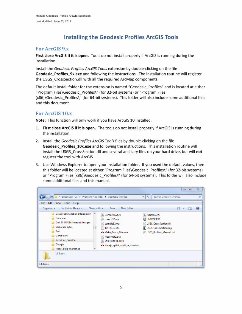
The default install folder for the extension is named “Geodesic_Profiles” and is located at either “Program Files\Geodesic_Profiles\” (for 32-bit systems) or “Program Files (x86)\Geodesic_Profiles\” (for 64-bit systems). This folder will also include some additional files and this document.
For ArcGIS 10.x
Note: This function will only work if you have ArcGIS 10 installed.
1. First close ArcGIS if it is open. The tools do not install properly if ArcGIS is running during the installation.
2. Install the Geodesic Profiles ArcGIS Tools files by double-clicking on the file Geodesic_Profiles_10x.exe and following the instructions. This installation routine will install the USGS_CrossSection.dll and several ancillary files on your hard drive, but will not register the tool with ArcGIS.
3. Use Windows Explorer to open your installation folder. If you used the default values, then this folder will be located at either “Program Files\Geodesic_Profiles\” (for 32-bit systems) or “Program Files (x86)\Geodesic_Profiles\” (for 64-bit systems). This folder will also include some additional files and this manual.
Manual: Geodesic Profiles ArcGIS Extension
Last Modified: June 13, 2017
6
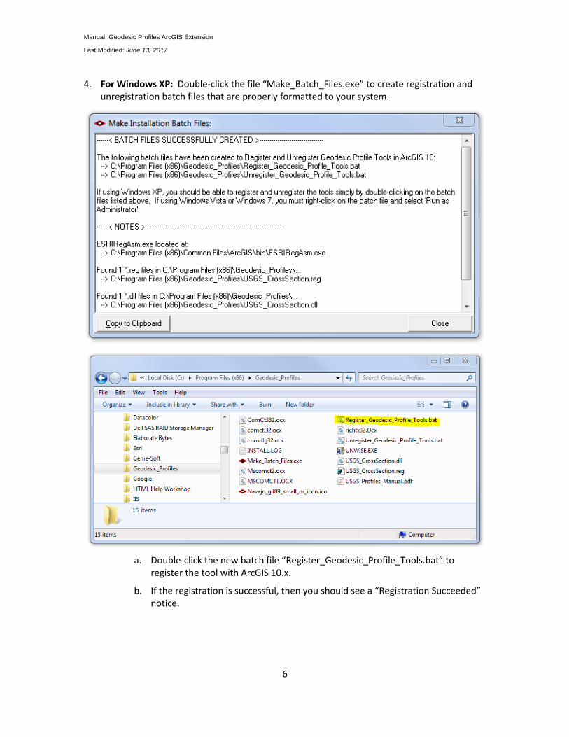
4. For Windows XP: Double-click the file “Make_Batch_Files.exe” to create registration and unregistration batch files that are properly formatted to your system.
a. Double-click the new batch file “Register_Geodesic_Profile_Tools.bat” to register the tool with ArcGIS 10.x.
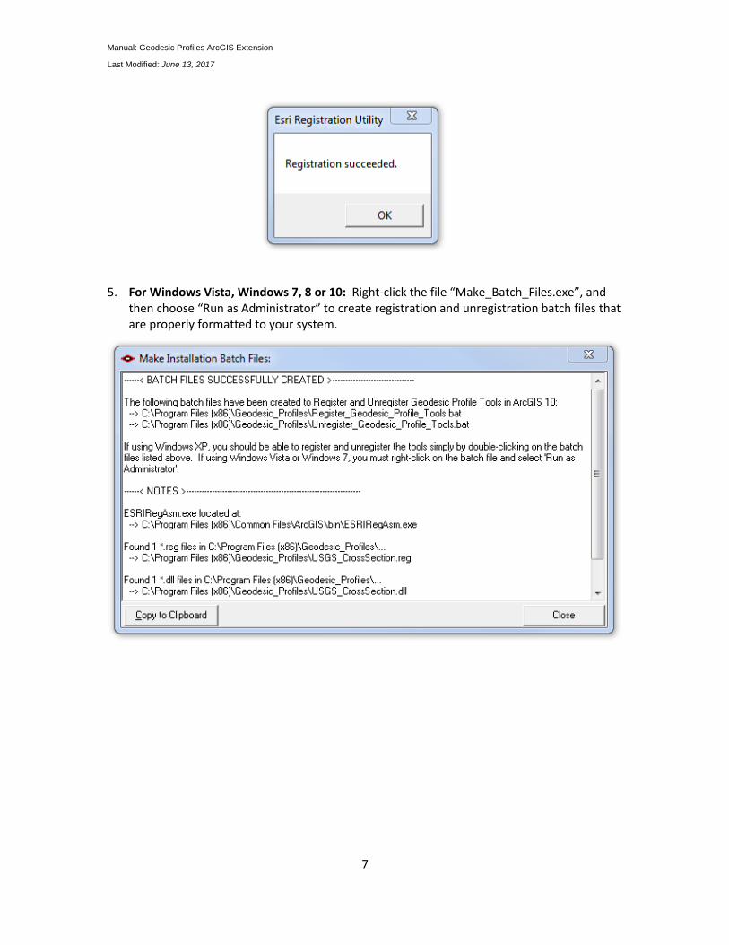
b. If the registration is successful, then you should see a “Registration Succeeded” notice.
Manual: Geodesic Profiles ArcGIS Extension
Last Modified: June 13, 2017
7
5. For Windows Vista, Windows 7, 8 or 10: Right-click the file “Make_Batch_Files.exe”, and then choose “Run as Administrator” to create registration and unregistration batch files that are properly formatted to your system.
Manual: Geodesic Profiles ArcGIS Extension
Last Modified: June 13, 2017
8
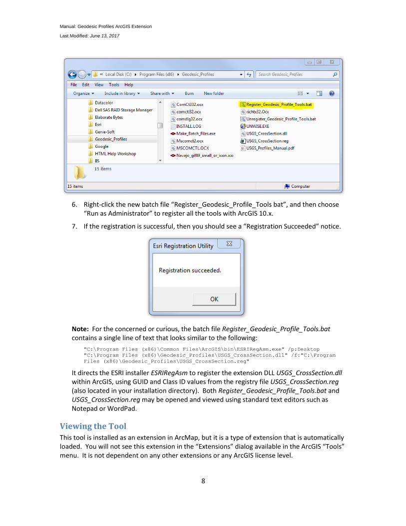
6. Right-click the new batch file “Register_Geodesic_Profile_Tools bat”, and then choose “Run as Administrator” to register all the tools with ArcGIS 10.x.
7. If the registration is successful, then you should see a “Registration Succeeded” notice.
Note: For the concerned or curious, the batch file Register_Geodesic_Profile_Tools.bat contains a single line of text that looks similar to the following:
"C:\Program Files (x86)\Common Files\ArcGIS\bin\ESRIRegAsm.exe" /p:Desktop
"C:\Program Files (x86)\Geodesic_Profiles\USGS_CrossSection.dll" /f:"C:\Program
Files (x86)\Geodesic_Profiles\USGS_CrossSection.reg"
It directs the ESRI installer ESRIRegAsm to register the extension DLL USGS_CrossSection.dll within ArcGIS, using GUID and Class ID values from the registry file USGS_CrossSection.reg (also located in your installation directory). Both Register_Geodesic_Profile_Tools.bat and USGS_CrossSection.reg may be opened and viewed using standard text editors such as Notepad or WordPad.
Viewing the Tool
This tool is installed as an extension in ArcMap, but it is a type of extension that is automatically loaded. You will not see this extension in the “Extensions” dialog available in the ArcGIS “Tools” menu. It is not dependent on any other extensions or any ArcGIS license level.
Manual: Geodesic Profiles ArcGIS Extension
Last Modified: June 13, 2017
9
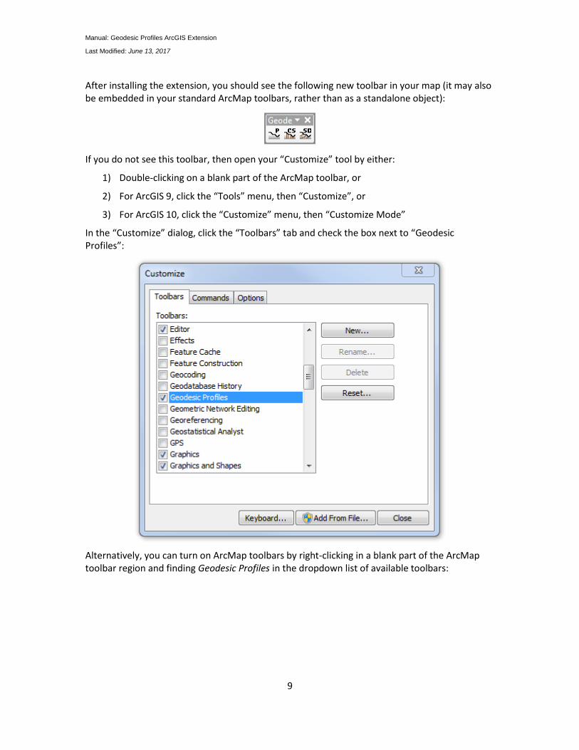
After installing the extension, you should see the following new toolbar in your map (it may also be embedded in your standard ArcMap toolbars, rather than as a standalone object):
If you do not see this toolbar, then open your “Customize” tool by either:
1) Double-clicking on a blank part of the ArcMap toolbar, or
2) For ArcGIS 9, click the “Tools” menu, then “Customize”, or
3) For ArcGIS 10, click the “Customize” menu, then “Customize Mode”
In the “Customize” dialog, click the “Toolbars” tab and check the box next to “Geodesic Profiles”:
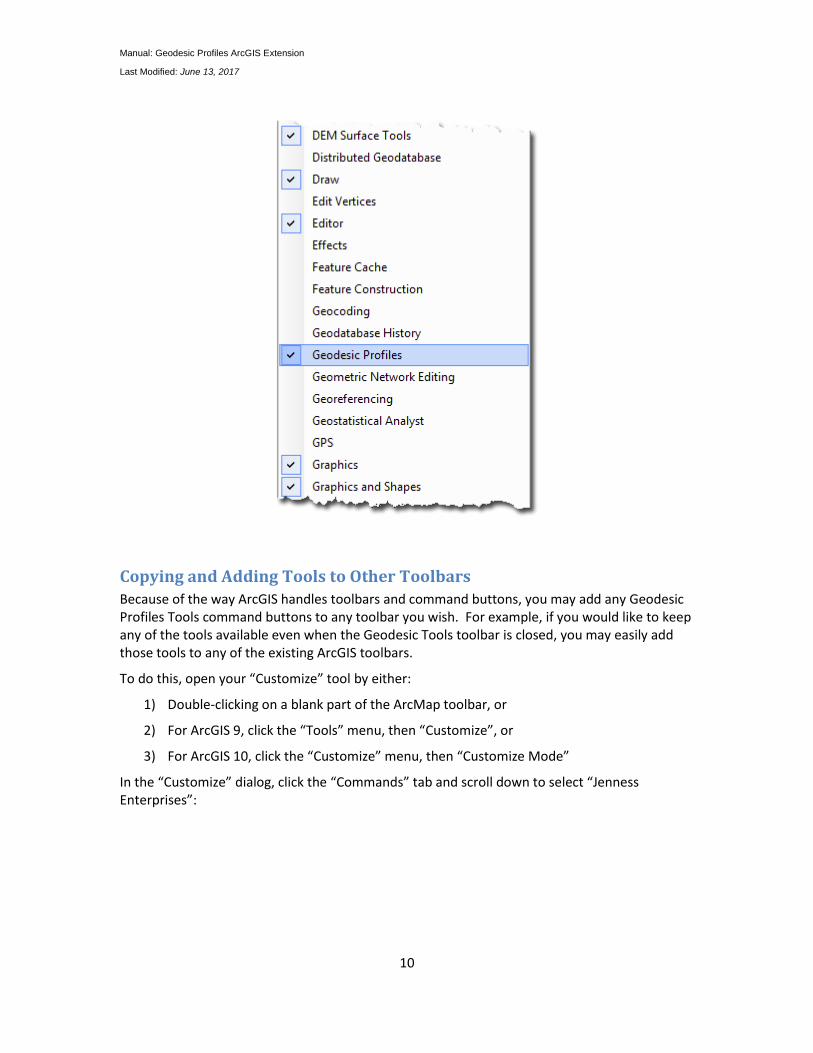
Alternatively, you can turn on ArcMap toolbars by right-clicking in a blank part of the ArcMap toolbar region and finding Geodesic Profiles in the dropdown list of available toolbars:
Manual: Geodesic Profiles ArcGIS Extension
Last Modified: June 13, 2017
10
Copying and Adding Tools to Other Toolbars
Because of the way ArcGIS handles toolbars and command buttons, you may add any Geodesic Profiles Tools command buttons to any toolbar you wish. For example, if you would like to keep any of the tools available even when the Geodesic Tools toolbar is closed, you may easily add those tools to any of the existing ArcGIS toolbars.
To do this, open your “Customize” tool by either:
1) Double-clicking on a blank part of the ArcMap toolbar, or
2) For ArcGIS 9, click the “Tools” menu, then “Customize”, or
3) For ArcGIS 10, click the “Customize” menu, then “Customize Mode”
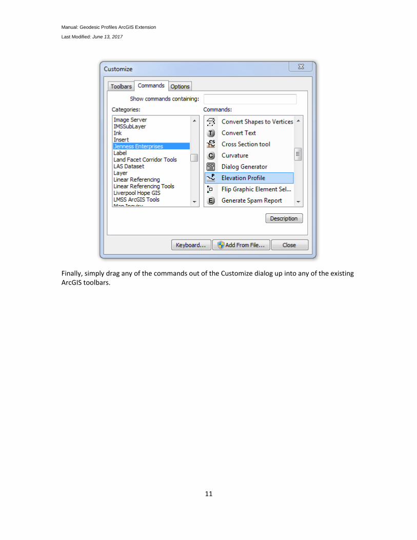
In the “Customize” dialog, click the “Commands” tab and scroll down to select “Jenness Enterprises”:
Manual: Geodesic Profiles ArcGIS Extension
Last Modified: June 13, 2017
11
Finally, simply drag any of the commands out of the Customize dialog up into any of the existing ArcGIS toolbars.
Manual: Geodesic Profiles ArcGIS Extension
Last Modified: June 13, 2017
12
Uninstalling the Geodesic Profiles ArcGIS Tools Extension
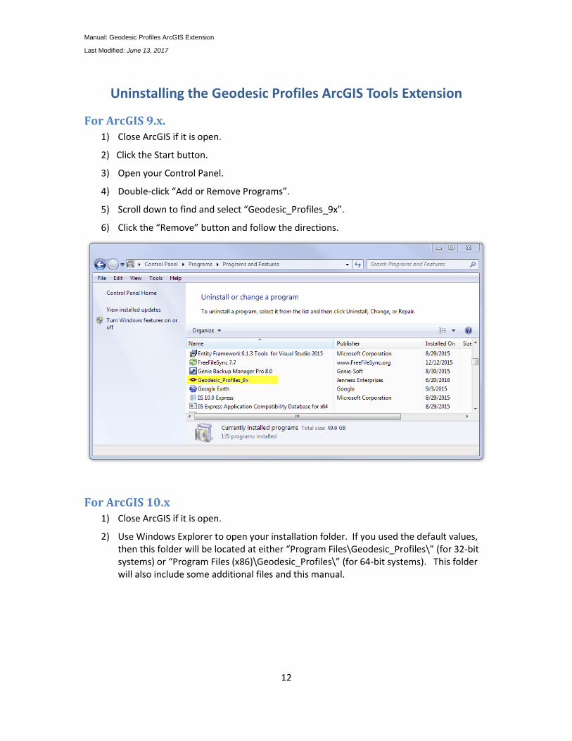
For ArcGIS 9.x.
1) Close ArcGIS if it is open.
2) Click the Start button.
3) Open your Control Panel.
4) Double-click “Add or Remove Programs”.
5) Scroll down to find and select “Geodesic_Profiles_9x”.
6) Click the “Remove” button and follow the directions.
For ArcGIS 10.x
1) Close ArcGIS if it is open.
2) Use Windows Explorer to open your installation folder. If you used the default values, then this folder will be located at either “Program Files\Geodesic_Profiles\” (for 32-bit systems) or “Program Files (x86)\Geodesic_Profiles\” (for 64-bit systems). This folder will also include some additional files and this manual.
Manual: Geodesic Profiles ArcGIS Extension
Last Modified: June 13, 2017
13
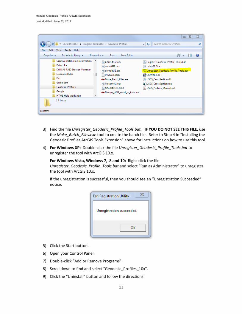
3) Find the file Unregister_Geodesic_Profile_Tools.bat. IF YOU DO NOT SEE THIS FILE, use the Make_Batch_Files.exe tool to create the batch file. Refer to Step 4 in “Installing the Geodesic Profiles ArcGIS Tools Extension” above for instructions on how to use this tool.
4) For Windows XP: Double-click the file Unregister_Geodesic_Profile_Tools.bat to unregister the tool with ArcGIS 10.x.
For Windows Vista, Windows 7, 8 and 10: Right-click the file Unregister_Geodesic_Profile_Tools.bat and select “Run as Administrator” to unregister the tool with ArcGIS 10.x.
If the unregistration is successful, then you should see an “Unregistration Succeeded” notice.
5) Click the Start button.
6) Open your Control Panel.
7) Double-click “Add or Remove Programs”.
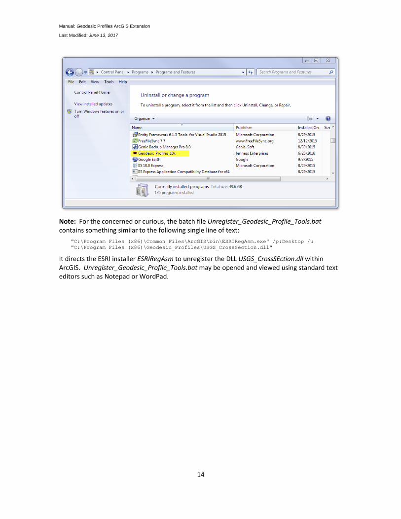
8) Scroll down to find and select “Geodesic_Profiles_10x”.
9) Click the “Uninstall” button and follow the directions.
Manual: Geodesic Profiles ArcGIS Extension
Last Modified: June 13, 2017
14
Note: For the concerned or curious, the batch file Unregister_Geodesic_Profile_Tools.bat contains something similar to the following single line of text:
"C:\Program Files (x86)\Common Files\ArcGIS\bin\ESRIRegAsm.exe" /p:Desktop /u
"C:\Program Files (x86)\Geodesic_Profiles\USGS_CrossSection.dll"
It directs the ESRI installer ESRIRegAsm to unregister the DLL USGS_CrossSEction.dll within ArcGIS. Unregister_Geodesic_Profile_Tools.bat may be opened and viewed using standard text editors such as Notepad or WordPad.
Manual: Geodesic Profiles ArcGIS Extension
Last Modified: June 13, 2017
15
Troubleshooting
If Any of the Tools Crash
If a tool crashes, you should see a dialog that tells us what script crashed and where it crashed. I would appreciate it if you could copy the text in that dialog, or simply take screenshots of the dialog and email them to me at [email protected]. Note: Please make sure that the line numbers are visible in the screenshots! The line numbers are located on the far right side of the text. Use the scrollbar at the bottom of the dialog to make the line numbers visible.
Error Log
In most cases, a crash will cause an error log to be produced in the Installation folder, named “Geodesic_Profiles_Error_Log_[Year][Month][Day]_[Hour][Minute][Second].txt”. For example, an error that occurred at exactly 5 seconds past 3:01pm, on October 1, 2015, would produce an error report named “Geodesic_Profiles_Error_Log_20151001_150105.txt”. Please send this error log to me at [email protected].
“Object variable or With block variable not set” Error:
If you open ArcMap and immediately see the error dialog appear with one or more error messages stating that “Object variable or With block variable not set”, then 90% of the time it is because ArcGIS was running when you installed the extension. The “Object” variable being referred to is the “Extension” object, and ArcGIS only sets that variable when it is initially opened.
The solution is usually to simply close ArcGIS and restart it. If that does not work, then:
1) Close ArcGIS
2) Reinstall the extension
3) Turn ArcGIS back on.
RICHTX32.OCX Error (also comct332.ocx, comdlg32.ocx, mscomct2.ocx, mscomctl.ocx, msstdfmt.dll errors):
If you see a line in the error dialog stating:
Component 'RICHTX32.OCX' or one of its dependencies not correctly registered: a file is
missing or invalid
Or if you see a similar error stating that one or more of the files comct332.ocx, comdlg32.ocx, mscomct2.ocx, mscomctl.ocx or msstdfmt.dll are missing or invalid, then simply follow the instructions for RICHTX32.OCX below, but substitute the appropriate file for RICHTX32.OCX.
This error is almost always due to the fact that new installations of Windows 7 and Windows Vista do not include a file that the extension expects to find. For example, the file “richtx32.ocx” is actually the “Rich Text Box” control that appears on some of the extension dialogs. The other OCX files refer to other common controls that might appear on the various extension dialogs.
The solution is to manually install the missing file (richtx32.ocx) yourself. Here is how to do it:
1) Open Windows Explorer and locate the file richtx32.ocx in your extension installation file.
Manual: Geodesic Profiles ArcGIS Extension
Last Modified: June 13, 2017
16
2) If you are running a 32-bit version of Windows, then copy richtx32.ocx to the directory
C:\Windows\System32\
If you are running a 64-bit version of Windows, then copy richtx32.ocx to the directory
C:\Windows\SysWOW64\
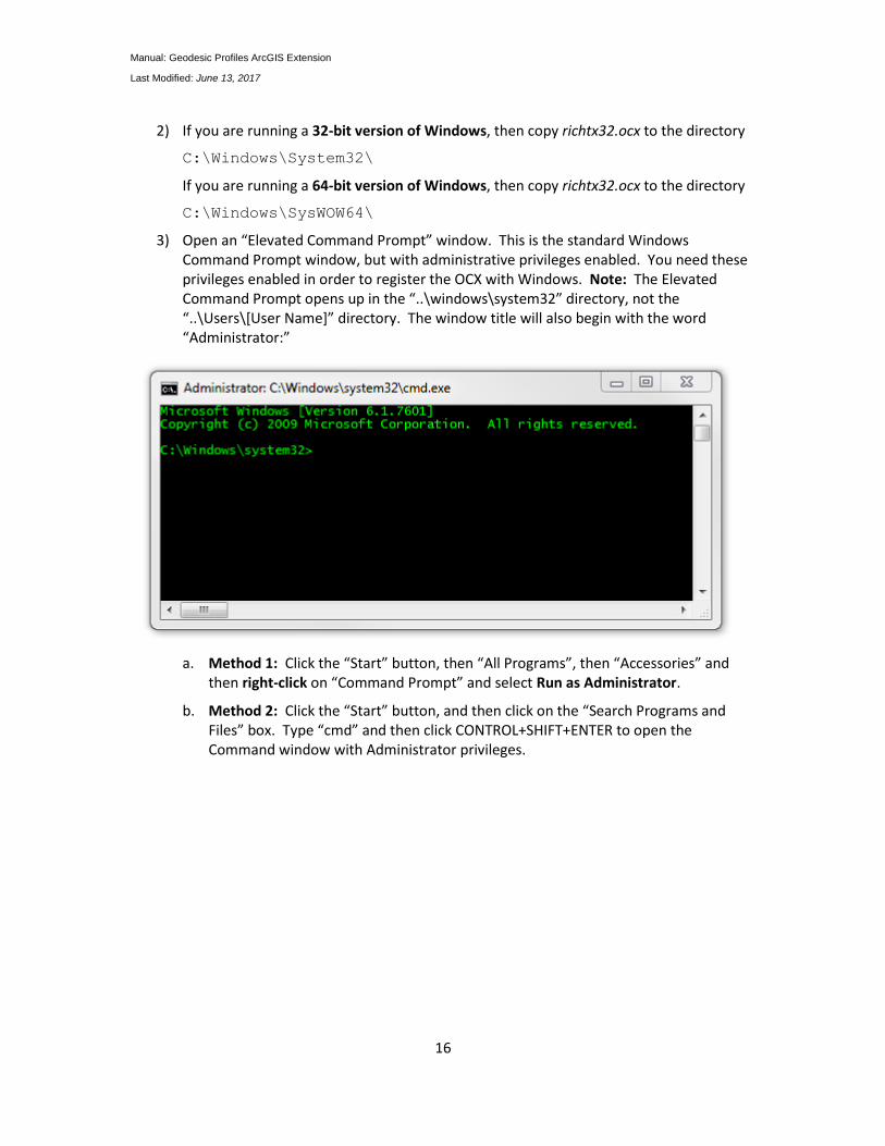
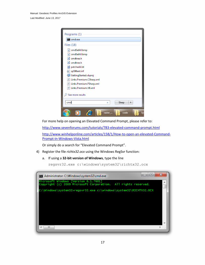
3) Open an “Elevated Command Prompt” window. This is the standard Windows Command Prompt window, but with administrative privileges enabled. You need these privileges enabled in order to register the OCX with Windows. Note: The Elevated Command Prompt opens up in the “..\windows\system32” directory, not the “..\Users\[User Name]” directory. The window title will also begin with the word “Administrator:”
a. Method 1: Click the “Start” button, then “All Programs”, then “Accessories” and then right-click on “Command Prompt” and select Run as Administrator.
b. Method 2: Click the “Start” button, and then click on the “Search Programs and Files” box. Type “cmd” and then click CONTROL+SHIFT+ENTER to open the Command window with Administrator privileges.
Manual: Geodesic Profiles ArcGIS Extension
Last Modified: June 13, 2017
17
For more help on opening an Elevated Command Prompt, please refer to:
http://www.sevenforums.com/tutorials/783-elevated-command-prompt.html
http://www.winhelponline.com/articles/158/1/How-to-open-an-elevated-Command-Prompt-in-Windows-Vista.html
Or simply do a search for “Elevated Command Prompt”.
4) Register the file richtx32.ocx using the Windows RegSvr function:
a. If using a 32-bit version of Windows, type the line
regsvr32.exe c:\windows\system32\richtx32.ocx
Manual: Geodesic Profiles ArcGIS Extension
Last Modified: June 13, 2017
18
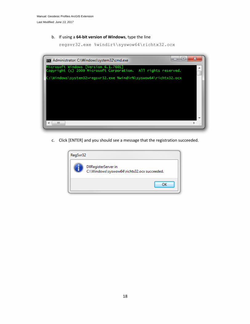
b. If using a 64-bit version of Windows, type the line
regsvr32.exe %windir%\syswow64\richtx32.ocx
c. Click [ENTER] and you should see a message that the registration succeeded.
Manual: Geodesic Profiles ArcGIS Extension
Last Modified: June 13, 2017
19
Using the Tools
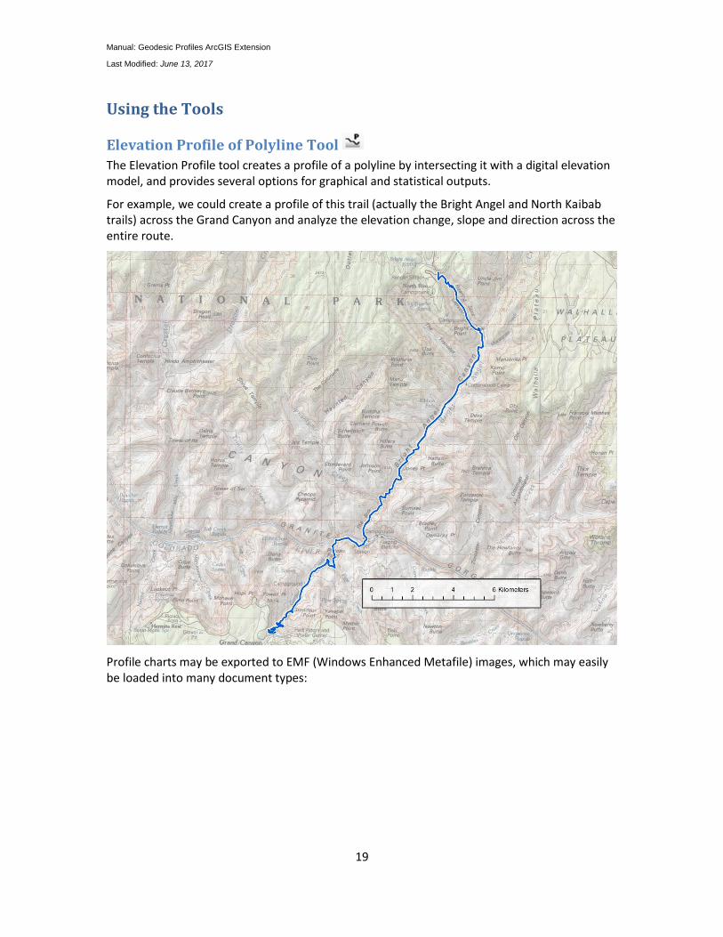
Elevation Profile of Polyline Tool
The Elevation Profile tool creates a profile of a polyline by intersecting it with a digital elevation model, and provides several options for graphical and statistical outputs.
For example, we could create a profile of this trail (actually the Bright Angel and North Kaibab trails) across the Grand Canyon and analyze the elevation change, slope and direction across the entire route.
Profile charts may be exported to EMF (Windows Enhanced Metafile) images, which may easily be loaded into many document types:
Manual: Geodesic Profiles ArcGIS Extension
Last Modified: June 13, 2017
20
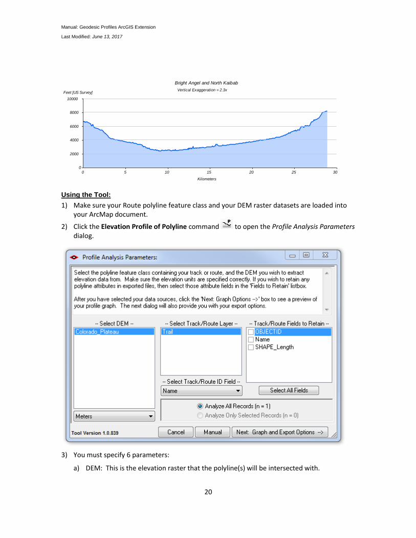
Using the Tool:
1) Make sure your Route polyline feature class and your DEM raster datasets are loaded into your ArcMap document.
2) Click the Elevation Profile of Polyline command to open the Profile Analysis Parameters dialog.
3) You must specify 6 parameters:
a) DEM: This is the elevation raster that the polyline(s) will be intersected with.
0
0
10000
2000
4000
6000
8000
Feet [US Survey]
305 10 15 20 25
Kilometers
Vertical Exaggeration = 2.3x
Bright Angel and North Kaibab
Manual: Geodesic Profiles ArcGIS Extension
Last Modified: June 13, 2017
21
b) Units: DEMs typically define elevation in meters or feet, but there is nothing in the dataset itself that explicitly defines the unit. Therefore you must specify the correct unit yourself. The tool defaults to Meters.
c) Track/Route Layer: This is the polyline feature class containing the route(s) to analyze.
d) Track/Route ID Field: This is the attribute used by the tool to label the graphs.
e) Track/Route Fields to Retain: The tool offers several output options for graphs and statistical tables. If you would like any of the original Track/Route attributes to be included in those statistical tables, then select those fields here. Note: The “Track/Route ID Field” will automatically be retained in all output datasets.
f) Whether to analyze all polylines, or only selected subset: If you have any polylines selected, then you have the option to restrict your analysis to only the selected subset. If you choose to analyze multiple polylines simultaneously, then the tool will overlay the graphs on each other.
Note: There may be issues regarding the coordinate systems of your data. If your data are in different geographic datums, then you may need to specify a geographic transformation. Please see Appendix A (p. 102) for details.
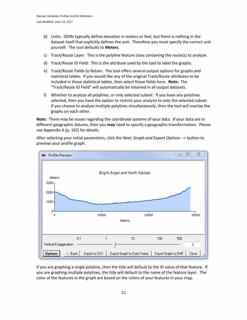
After selecting your initial parameters, click the Next: Graph and Export Options --> button to preview your profile graph.
If you are graphing a single polyline, then the title will default to the ID value of that feature. If you are graphing multiple polylines, the title will default to the name of the feature layer. The color of the features in the graph are based on the colors of your features in your map.
Manual: Geodesic Profiles ArcGIS Extension
Last Modified: June 13, 2017
22
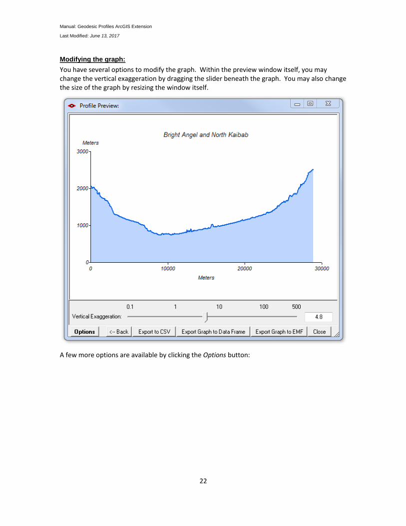
Modifying the graph:
You have several options to modify the graph. Within the preview window itself, you may change the vertical exaggeration by dragging the slider beneath the graph. You may also change the size of the graph by resizing the window itself.
A few more options are available by clicking the Options button:
Manual: Geodesic Profiles ArcGIS Extension
Last Modified: June 13, 2017
23
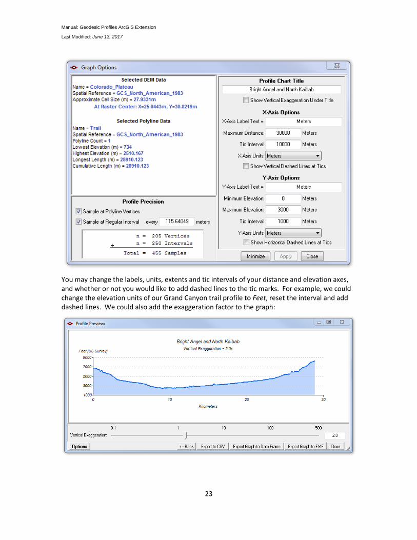
You may change the labels, units, extents and tic intervals of your distance and elevation axes, and whether or not you would like to add dashed lines to the tic marks. For example, we could change the elevation units of our Grand Canyon trail profile to Feet, reset the interval and add dashed lines. We could also add the exaggeration factor to the graph:
Manual: Geodesic Profiles ArcGIS Extension
Last Modified: June 13, 2017
24
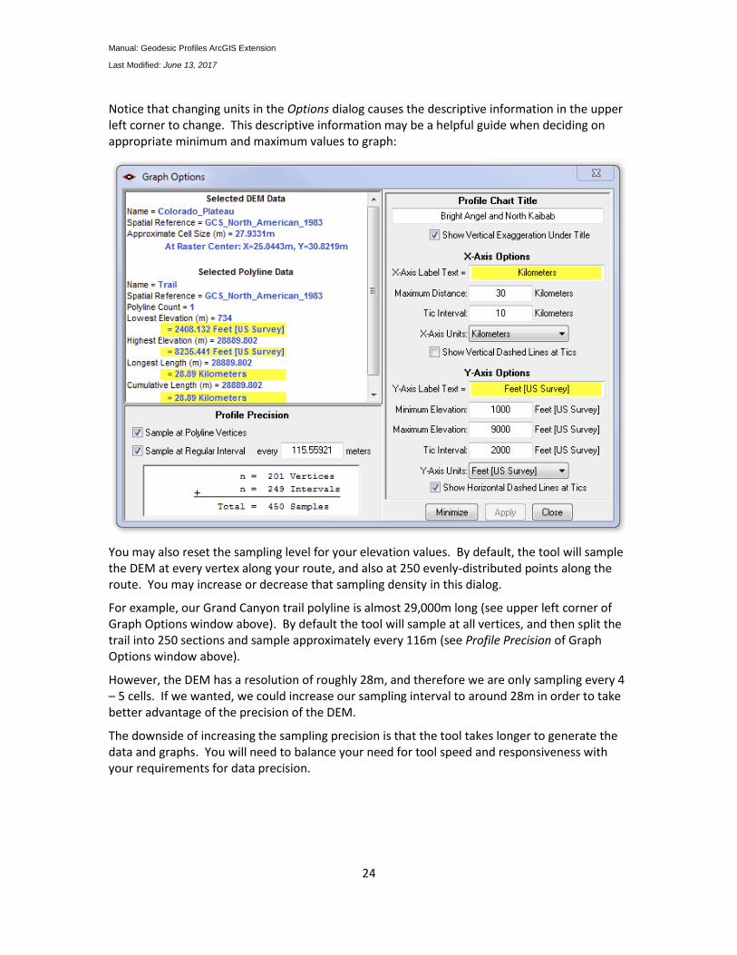
Notice that changing units in the Options dialog causes the descriptive information in the upper left corner to change. This descriptive information may be a helpful guide when deciding on appropriate minimum and maximum values to graph:
You may also reset the sampling level for your elevation values. By default, the tool will sample the DEM at every vertex along your route, and also at 250 evenly-distributed points along the route. You may increase or decrease that sampling density in this dialog.
For example, our Grand Canyon trail polyline is almost 29,000m long (see upper left corner of Graph Options window above). By default the tool will sample at all vertices, and then split the trail into 250 sections and sample approximately every 116m (see Profile Precision of Graph Options window above).
However, the DEM has a resolution of roughly 28m, and therefore we are only sampling every 4 – 5 cells. If we wanted, we could increase our sampling interval to around 28m in order to take better advantage of the precision of the DEM.
The downside of increasing the sampling precision is that the tool takes longer to generate the data and graphs. You will need to balance your need for tool speed and responsiveness with your requirements for data precision.
Manual: Geodesic Profiles ArcGIS Extension
Last Modified: June 13, 2017
25
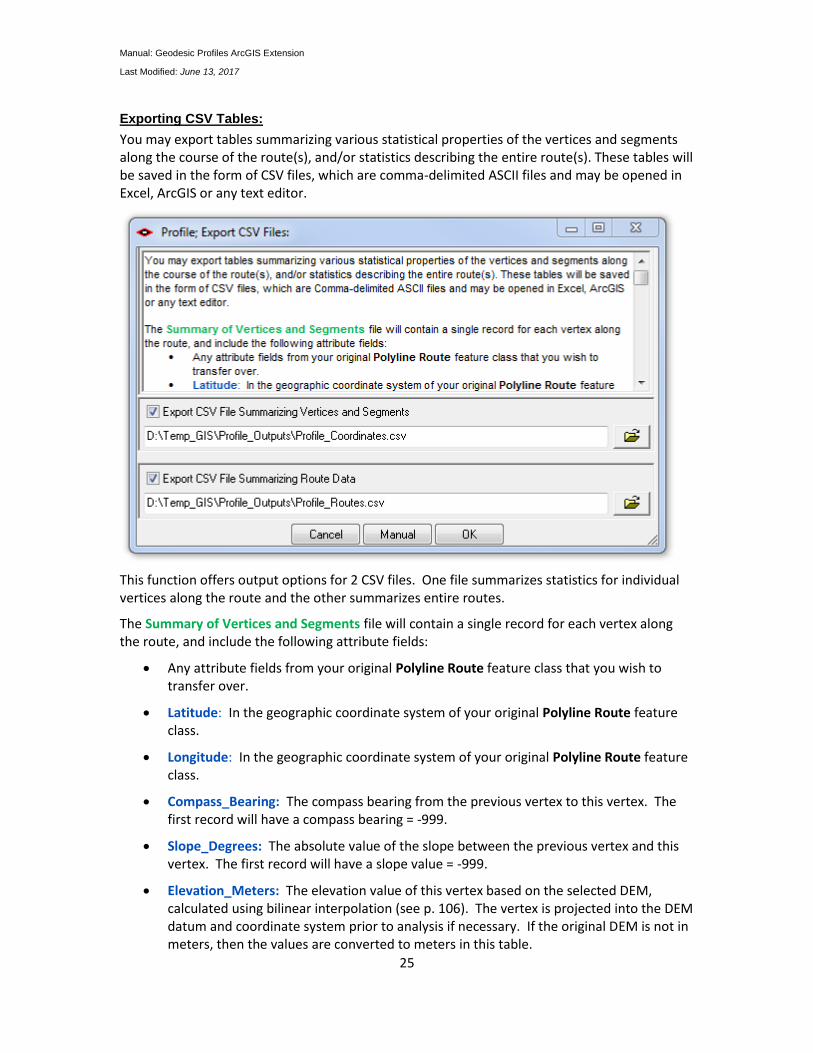
Exporting CSV Tables:
You may export tables summarizing various statistical properties of the vertices and segments along the course of the route(s), and/or statistics describing the entire route(s). These tables will be saved in the form of CSV files, which are comma-delimited ASCII files and may be opened in Excel, ArcGIS or any text editor.
This function offers output options for 2 CSV files. One file summarizes statistics for individual vertices along the route and the other summarizes entire routes.
The Summary of Vertices and Segments file will contain a single record for each vertex along the route, and include the following attribute fields:
Any attribute fields from your original Polyline Route feature class that you wish to transfer over.
Latitude: In the geographic coordinate system of your original Polyline Route feature class.
Longitude: In the geographic coordinate system of your original Polyline Route feature class.
Compass_Bearing: The compass bearing from the previous vertex to this vertex. The first record will have a compass bearing = -999.
Slope_Degrees: The absolute value of the slope between the previous vertex and this vertex. The first record will have a slope value = -999.
Elevation_Meters: The elevation value of this vertex based on the selected DEM, calculated using bilinear interpolation (see p. 106). The vertex is projected into the DEM datum and coordinate system prior to analysis if necessary. If the original DEM is not in meters, then the values are converted to meters in this table.

Manual: Geodesic Profiles ArcGIS Extension
Last Modified: June 13, 2017
26
Segment_Geodesic_Distance_Meters: The distance, in meters, between the previous vertex and this one, calculated using Vincenty's algorithms to estimate geodesic distances over the original Polygon Route feature class spheroid (see Vincenty 1975; also p. 124 of this manual).
Segment_Surface_Distance_Meters: The surface distance, in meters, between the previous vertex and this one, calculated using the Pythagorean theorem to determine the hypotenuse of the triangle formed by the change in elevation and the geodesic distance.
Cumulative_Proportion: The proportion of the original route at this vertex. This proportion is based on the surface distance of the line, not the geodesic distance.
Cumulative_Geodesic_Distance_Meters: The total geodesic distance along the route up to this vertex.
Cumulative_Surface_Distance_Meters: The total surface distance along the route up to this vertex.
X_Original_Units: The X-coordinate in the original units of the source Polyline Route feature class. For example, if the source data were in UTM coordinates, then this value would be the vertex Easting value.
Y_Original_Units: The Y-coordinate in the original units of the source Polyline Route feature class. For example, if the source data were in UTM coordinates, then this value would be the vertex Northing value.
Elevation_Original_Units: The elevation value in the original units of the source DEM.
Exaggeration_Factor: The exaggeration factor used to adjust the dimensions of the profile graph. This may be useful if you wish to generate a profile graph from these points in some other software package such as R.
Exaggerated_Elev: The elevation of the vertex after being multiplied by the exaggeration factor. This is the value that is actually being plotted on the graph, and this value may also be useful if you wish to generate a profile graph from these points in some other software package.
The Summary of Routes file will contain a single record for each route analyzed, and will include the following attribute fields:
Any attribute fields from your original Polyline Route feature class that you wish to transfer over.
Sample_Points: The number of DEM values sampled to generate the statistics for this polyline.
Start_Latitude: In the geographic coordinate system of your original Polyline Route feature class.
Start_Longitude: In the geographic coordinate system of your original Polyline Route feature class.
Manual: Geodesic Profiles ArcGIS Extension
Last Modified: June 13, 2017
27
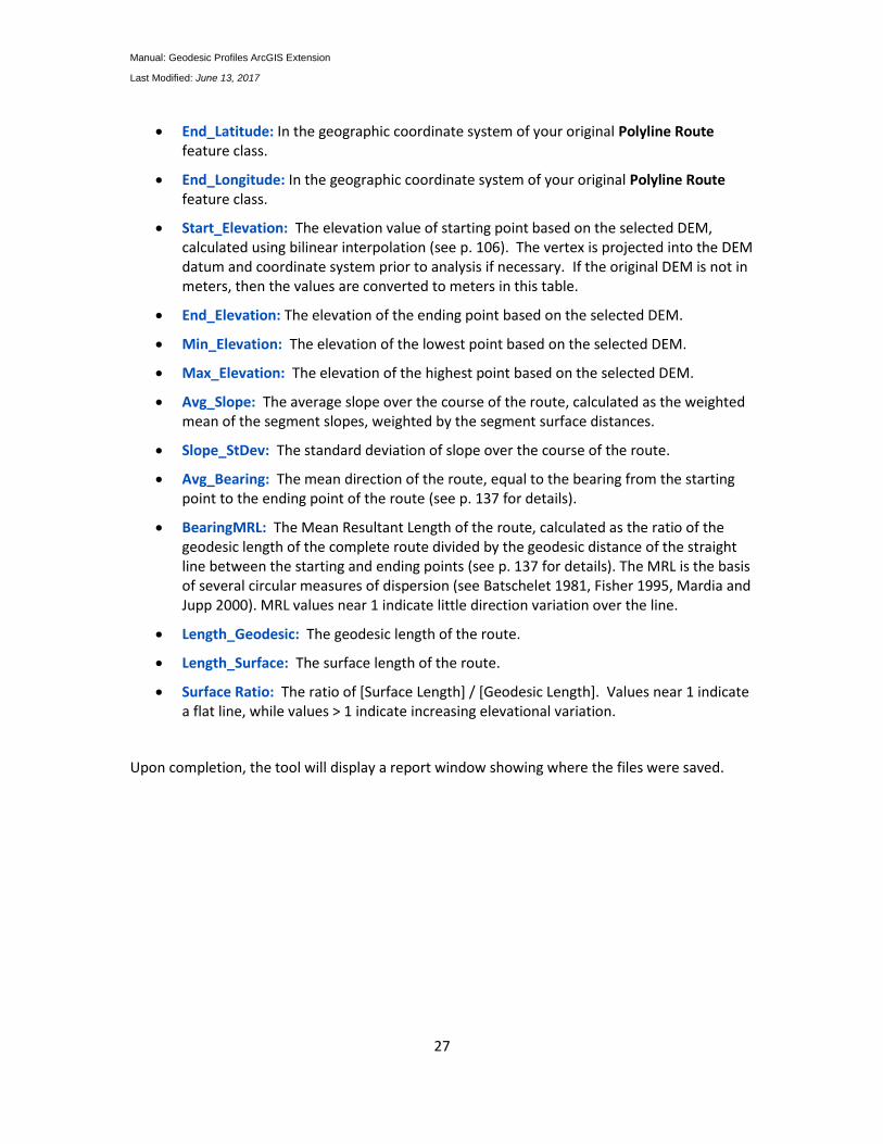
End_Latitude: In the geographic coordinate system of your original Polyline Route feature class.
End_Longitude: In the geographic coordinate system of your original Polyline Route feature class.
Start_Elevation: The elevation value of starting point based on the selected DEM, calculated using bilinear interpolation (see p. 106). The vertex is projected into the DEM datum and coordinate system prior to analysis if necessary. If the original DEM is not in meters, then the values are converted to meters in this table.
End_Elevation: The elevation of the ending point based on the selected DEM.
Min_Elevation: The elevation of the lowest point based on the selected DEM.
Max_Elevation: The elevation of the highest point based on the selected DEM.
Avg_Slope: The average slope over the course of the route, calculated as the weighted mean of the segment slopes, weighted by the segment surface distances.
Slope_StDev: The standard deviation of slope over the course of the route.
Avg_Bearing: The mean direction of the route, equal to the bearing from the starting point to the ending point of the route (see p. 137 for details).
BearingMRL: The Mean Resultant Length of the route, calculated as the ratio of the geodesic length of the complete route divided by the geodesic distance of the straight line between the starting and ending points (see p. 137 for details). The MRL is the basis of several circular measures of dispersion (see Batschelet 1981, Fisher 1995, Mardia and Jupp 2000). MRL values near 1 indicate little direction variation over the line.
Length_Geodesic: The geodesic length of the route.
Length_Surface: The surface length of the route.
Surface Ratio: The ratio of [Surface Length] / [Geodesic Length]. Values near 1 indicate a flat line, while values > 1 indicate increasing elevational variation.
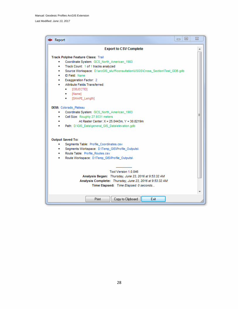
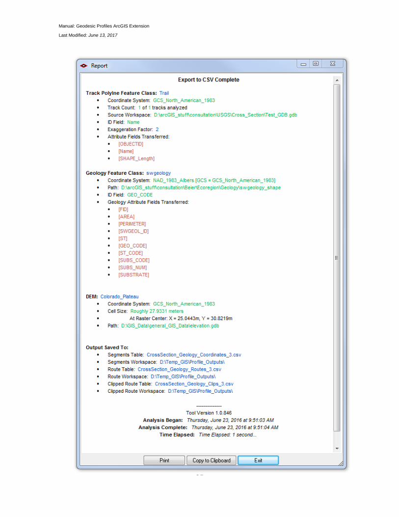
Upon completion, the tool will display a report window showing where the files were saved.
Manual: Geodesic Profiles ArcGIS Extension
Last Modified: June 13, 2017
28
Manual: Geodesic Profiles ArcGIS Extension
Last Modified: June 13, 2017
29
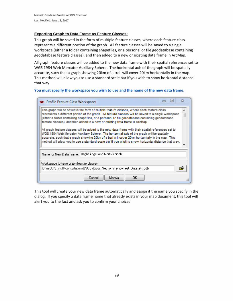
Exporting Graph to Data Frame as Feature Classes:
This graph will be saved in the form of multiple feature classes, where each feature class represents a different portion of the graph. All feature classes will be saved to a single workspace (either a folder containing shapefiles, or a personal or file geodatabase containing geodatabase feature classes), and then added to a new or existing data frame in ArcMap.
All graph feature classes will be added to the new data frame with their spatial references set to WGS 1984 Web Mercator Auxiliary Sphere. The horizontal axis of the graph will be spatially accurate, such that a graph showing 20km of a trail will cover 20km horizontally in the map. This method will allow you to use a standard scale bar if you wish to show horizontal distance that way.
You must specify the workspace you wish to use and the name of the new data frame.
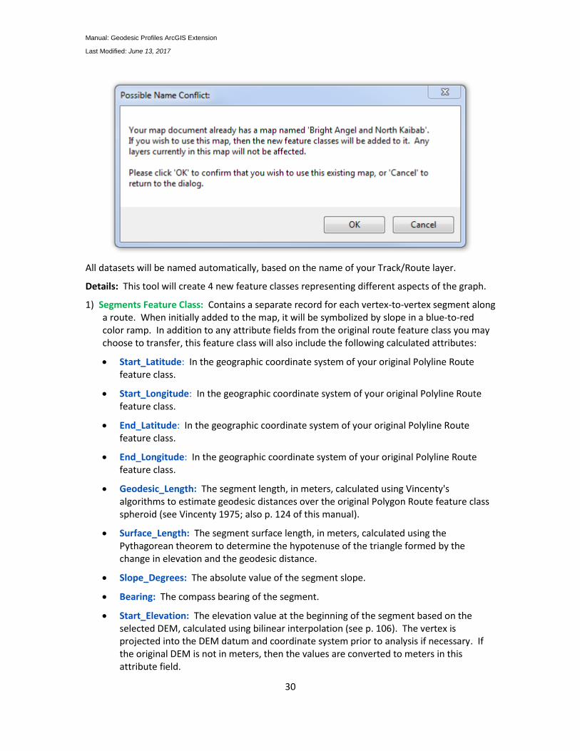
This tool will create your new data frame automatically and assign it the name you specify in the dialog. If you specify a data frame name that already exists in your map document, this tool will alert you to the fact and ask you to confirm your choice:
Manual: Geodesic Profiles ArcGIS Extension
Last Modified: June 13, 2017
30
All datasets will be named automatically, based on the name of your Track/Route layer.
Details: This tool will create 4 new feature classes representing different aspects of the graph.
1) Segments Feature Class: Contains a separate record for each vertex-to-vertex segment along a route. When initially added to the map, it will be symbolized by slope in a blue-to-red color ramp. In addition to any attribute fields from the original route feature class you may choose to transfer, this feature class will also include the following calculated attributes:
Start_Latitude: In the geographic coordinate system of your original Polyline Route feature class.
Start_Longitude: In the geographic coordinate system of your original Polyline Route feature class.
End_Latitude: In the geographic coordinate system of your original Polyline Route feature class.
End_Longitude: In the geographic coordinate system of your original Polyline Route feature class.
Geodesic_Length: The segment length, in meters, calculated using Vincenty's algorithms to estimate geodesic distances over the original Polygon Route feature class spheroid (see Vincenty 1975; also p. 124 of this manual).
Surface_Length: The segment surface length, in meters, calculated using the Pythagorean theorem to determine the hypotenuse of the triangle formed by the change in elevation and the geodesic distance.
Slope_Degrees: The absolute value of the segment slope.
Bearing: The compass bearing of the segment.
Start_Elevation: The elevation value at the beginning of the segment based on the selected DEM, calculated using bilinear interpolation (see p. 106). The vertex is projected into the DEM datum and coordinate system prior to analysis if necessary. If the original DEM is not in meters, then the values are converted to meters in this attribute field.
Manual: Geodesic Profiles ArcGIS Extension
Last Modified: June 13, 2017
31
Mid_Elevation: The elevation value at the centerpoint of the segment.
End_Elevation: The elevation value at the end of the segment.
End_Proportion: The proportion of the original route at the segment endpoint. This proportion is based on the surface distance of the line, not the geodesic distance. Values will range from 0 to 1.
Total_Geodesic_Distance: The total geodesic distance, in meters, along the route up to the end of this segment.
Total_Surface_Distance: The total surface distance, in meters, along the route up to the end of this segment.
2) Polyline Feature Class: Contains a separate record for each route showing the profile of the route over the DEM. When initially added to the map, it will be symbolized by ID value based on the ID field you select. If you do not select an ID field, it will be symbolized by the Feature Object ID of the original route. In addition to any attribute fields from the original route feature class you may choose to transfer, this feature class will also include the following calculated attributes:
Sample_Points: The number of DEM values sampled to generate the statistics for this polyline.
Start_Latitude: In the geographic coordinate system of your original Polyline Route feature class.
Start_Longitude: In the geographic coordinate system of your original Polyline Route feature class.
End_Latitude: In the geographic coordinate system of your original Polyline Route feature class.
End_Longitude: In the geographic coordinate system of your original Polyline Route feature class.
Start_Elevation: The elevation value of starting point based on the selected DEM, calculated using bilinear interpolation (see p. 106). The vertex is projected into the DEM datum and coordinate system prior to analysis if necessary. If the original DEM is not in meters, then the values are converted to meters in this table.
End_Elevation: The elevation of the ending point based on the selected DEM.
Min_Elevation: The elevation of the lowest point based on the selected DEM.
Max_Elevation: The elevation of the highest point based on the selected DEM.
Avg_Slope: The average slope over the course of the route, calculated as the weighted mean of the segment slopes, weighted by the segment surface distances.
Slope_StDev: The standard deviation of slope over the course of the route.
Avg_Bearing: The mean direction of the route, equal to the bearing from the starting point to the ending point of the route (see p. 137 for details).
Manual: Geodesic Profiles ArcGIS Extension
Last Modified: June 13, 2017
32
BearingMRL: The Mean Resultant Length of the route, calculated as the ratio of the geodesic length of the complete route divided by the geodesic distance of the straight line between the starting and ending points (see p. 137 for details). The MRL is the basis of several circular measures of dispersion (see Batschelet 1981, Fisher 1995, Mardia and Jupp 2000). MRL values near 1 indicate little direction variation over the line.
Length_Geodesic: The geodesic length of the route.
Length_Surface: The surface length of the route.
Surface Ratio: The ratio of [Surface Length] / [Geodesic Length]. Values near 1 indicate a flat line, while values > 1 indicate increasing elevational variation.
3) Polygon Feature Class: Similar to the Polyline Feature Class, except that it symbolizes the route using a polygon to symbolize the portion of the graph underneath the route profile. Contains a separate record for each route. When initially added to the map, it will be symbolized by ID value based on the ID field you select. If you do not select an ID field, it will be symbolized by the Feature Object ID of the original route. This feature class will contain exactly the same attribute fields and values as the Polyline Feature Class described above.
4) Graph_Lines: Simply shows the reference lines of the graph, including axes, tick marks and horizontal/vertical references. Attribute values include the name of the line (X-Axis, Y-Axis, X-Tic, Y-Tic, X-Reference and Y-Reference), and a label value for that line.
This tool will also add graphic text boxes for label values, axis names and the chart title. Note: These graphics can be converted to annotation by right-clicking data frame name and choosing "Convert Labels to Annotation". This option helps the labels look better if you add the graph to a layout. See also a known issue with exported graphic text on p. 96.
Manual: Geodesic Profiles ArcGIS Extension
Last Modified: June 13, 2017
33
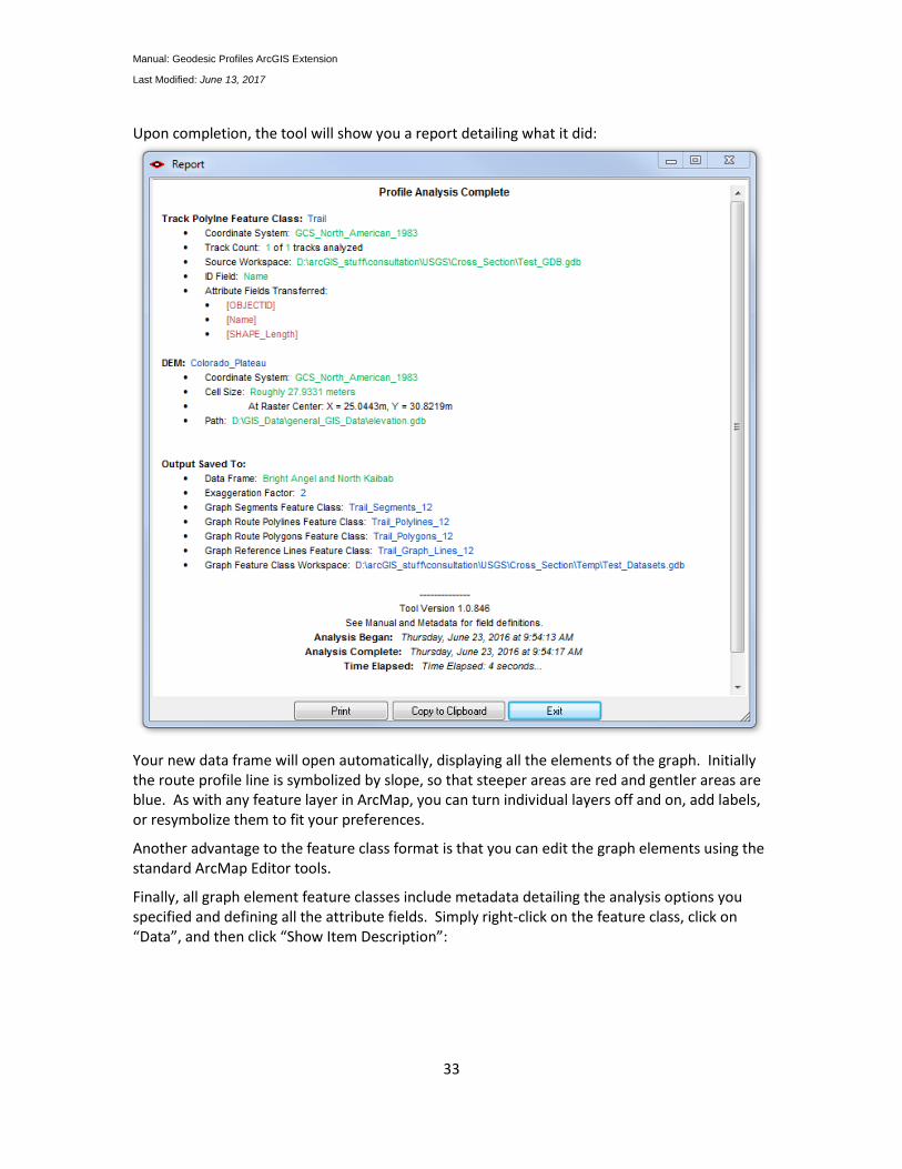
Upon completion, the tool will show you a report detailing what it did:
Your new data frame will open automatically, displaying all the elements of the graph. Initially the route profile line is symbolized by slope, so that steeper areas are red and gentler areas are blue. As with any feature layer in ArcMap, you can turn individual layers off and on, add labels, or resymbolize them to fit your preferences.
Another advantage to the feature class format is that you can edit the graph elements using the standard ArcMap Editor tools.
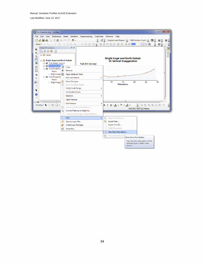
Finally, all graph element feature classes include metadata detailing the analysis options you specified and defining all the attribute fields. Simply right-click on the feature class, click on “Data”, and then click “Show Item Description”:
Manual: Geodesic Profiles ArcGIS Extension
Last Modified: June 13, 2017
34
Manual: Geodesic Profiles ArcGIS Extension
Last Modified: June 13, 2017
35
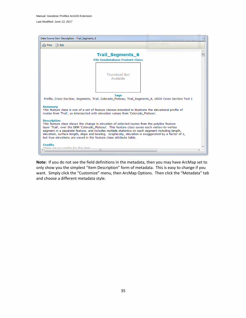
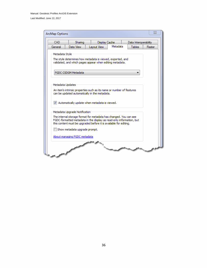
Note: If you do not see the field definitions in the metadata, then you may have ArcMap set to only show you the simplest “Item Description” form of metadata. This is easy to change if you want. Simply click the “Customize” menu, then ArcMap Options. Then click the “Metadata” tab and choose a different metadata style.
Manual: Geodesic Profiles ArcGIS Extension
Last Modified: June 13, 2017
36
Manual: Geodesic Profiles ArcGIS Extension
Last Modified: June 13, 2017
37
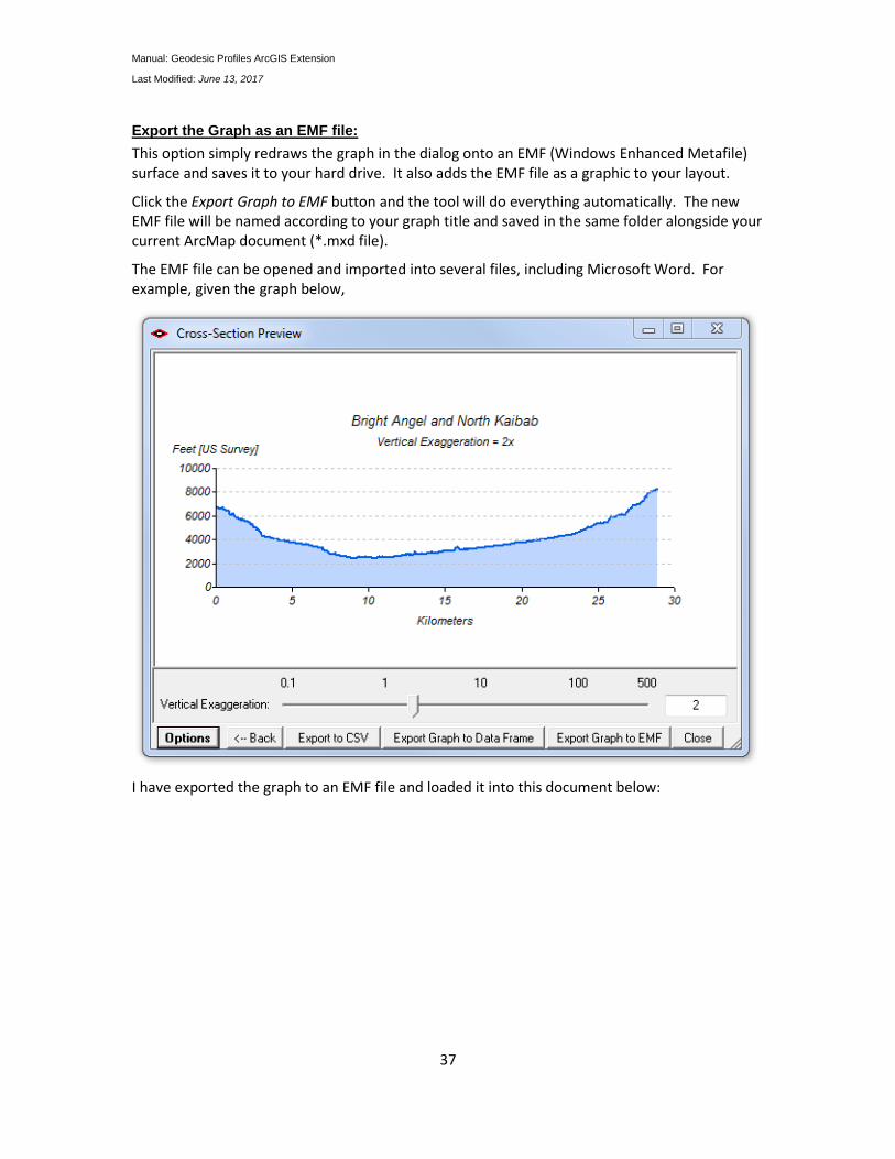
Export the Graph as an EMF file:
This option simply redraws the graph in the dialog onto an EMF (Windows Enhanced Metafile) surface and saves it to your hard drive. It also adds the EMF file as a graphic to your layout.
Click the Export Graph to EMF button and the tool will do everything automatically. The new EMF file will be named according to your graph title and saved in the same folder alongside your current ArcMap document (*.mxd file).
The EMF file can be opened and imported into several files, including Microsoft Word. For example, given the graph below,
I have exported the graph to an EMF file and loaded it into this document below:
Manual: Geodesic Profiles ArcGIS Extension
Last Modified: June 13, 2017
38
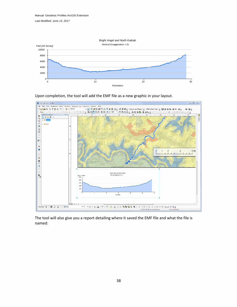
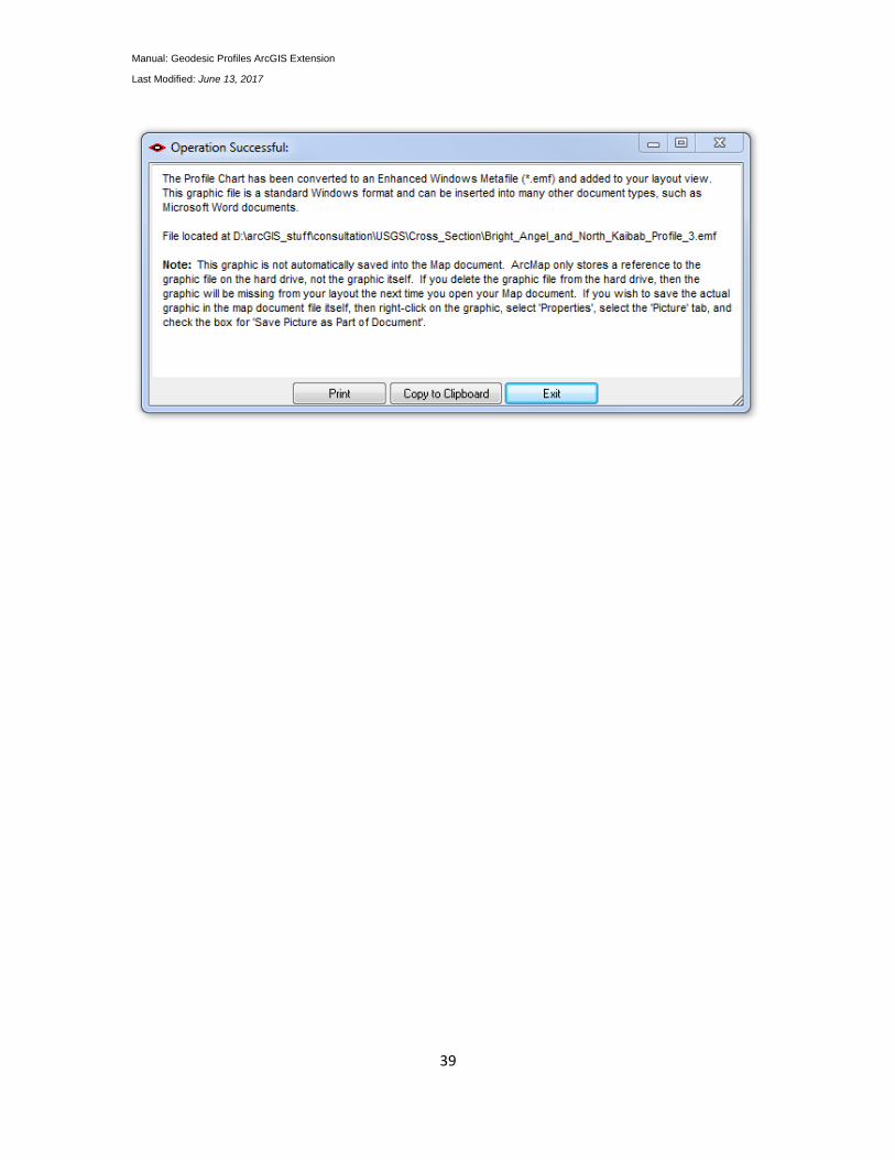
Upon completion, the tool will add the EMF file as a new graphic in your layout.
The tool will also give you a report detailing where it saved the EMF file and what the file is named:
0
0
10000
2000
4000
6000
8000
Feet [US Survey]
3010 20
Kilometers
Vertical Exaggeration = 2x
Bright Angel and North Kaibab
Manual: Geodesic Profiles ArcGIS Extension
Last Modified: June 13, 2017
39
Manual: Geodesic Profiles ArcGIS Extension
Last Modified: June 13, 2017
40
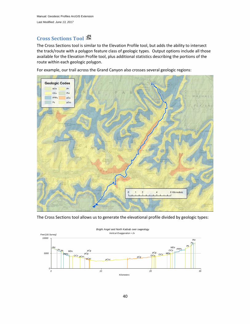
Cross Sections Tool
The Cross Sections tool is similar to the Elevation Profile tool, but adds the ability to intersect the track/route with a polygon feature class of geologic types. Output options include all those available for the Elevation Profile tool, plus additional statistics describing the portions of the route within each geologic polygon.
For example, our trail across the Grand Canyon also crosses several geologic regions:
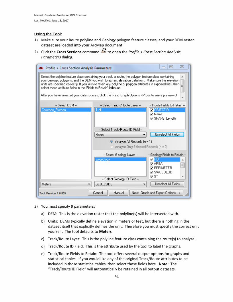
The Cross Sections tool allows us to generate the elevational profile divided by geologic types:
0
0
10000
5000
Feet [US Survey]
3010 20
Kilometers
Vertical Exaggeration = 2x
PktPc Ph
PPPs
MDs
OCs pCsc
pCg
pCsc
pCg
pCsc
pCgOCs
pCgOCs
MDs
OCs
MDsPPPs
Ph
Pc
Pkt
Bright Angel and North Kaibab over swgeology
Manual: Geodesic Profiles ArcGIS Extension
Last Modified: June 13, 2017
41
Using the Tool:
1) Make sure your Route polyline and Geology polygon feature classes, and your DEM raster dataset are loaded into your ArcMap document.
2) Click the Cross Sections command to open the Profile + Cross Section Analysis Parameters dialog.
3) You must specify 9 parameters:
a) DEM: This is the elevation raster that the polyline(s) will be intersected with.
b) Units: DEMs typically define elevation in meters or feet, but there is nothing in the dataset itself that explicitly defines the unit. Therefore you must specify the correct unit yourself. The tool defaults to Meters.
c) Track/Route Layer: This is the polyline feature class containing the route(s) to analyze.
d) Track/Route ID Field: This is the attribute used by the tool to label the graphs.
e) Track/Route Fields to Retain: The tool offers several output options for graphs and statistical tables. If you would like any of the original Track/Route attributes to be included in those statistical tables, then select those fields here. Note: The “Track/Route ID Field” will automatically be retained in all output datasets.
Manual: Geodesic Profiles ArcGIS Extension
Last Modified: June 13, 2017
42
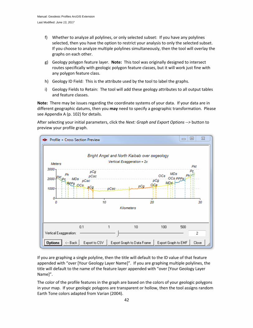
f) Whether to analyze all polylines, or only selected subset: If you have any polylines selected, then you have the option to restrict your analysis to only the selected subset. If you choose to analyze multiple polylines simultaneously, then the tool will overlay the graphs on each other.
g) Geology polygon feature layer. Note: This tool was originally designed to intersect routes specifically with geologic polygon feature classes, but it will work just fine with any polygon feature class.
h) Geology ID Field: This is the attribute used by the tool to label the graphs.
i) Geology Fields to Retain: The tool will add these geology attributes to all output tables and feature classes.
Note: There may be issues regarding the coordinate systems of your data. If your data are in different geographic datums, then you may need to specify a geographic transformation. Please see Appendix A (p. 102) for details.
After selecting your initial parameters, click the Next: Graph and Export Options --> button to preview your profile graph.
If you are graphing a single polyline, then the title will default to the ID value of that feature appended with “over [Your Geology Layer Name]”. If you are graphing multiple polylines, the title will default to the name of the feature layer appended with “over [Your Geology Layer Name]”.
The color of the profile features in the graph are based on the colors of your geologic polygons in your map. If your geologic polygons are transparent or hollow, then the tool assigns random Earth Tone colors adapted from Varian (2004).
Manual: Geodesic Profiles ArcGIS Extension
Last Modified: June 13, 2017
43
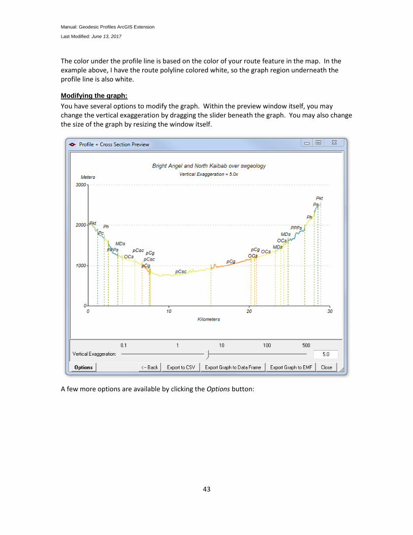
The color under the profile line is based on the color of your route feature in the map. In the example above, I have the route polyline colored white, so the graph region underneath the profile line is also white.
Modifying the graph:
You have several options to modify the graph. Within the preview window itself, you may change the vertical exaggeration by dragging the slider beneath the graph. You may also change the size of the graph by resizing the window itself.
A few more options are available by clicking the Options button:
Manual: Geodesic Profiles ArcGIS Extension
Last Modified: June 13, 2017
44
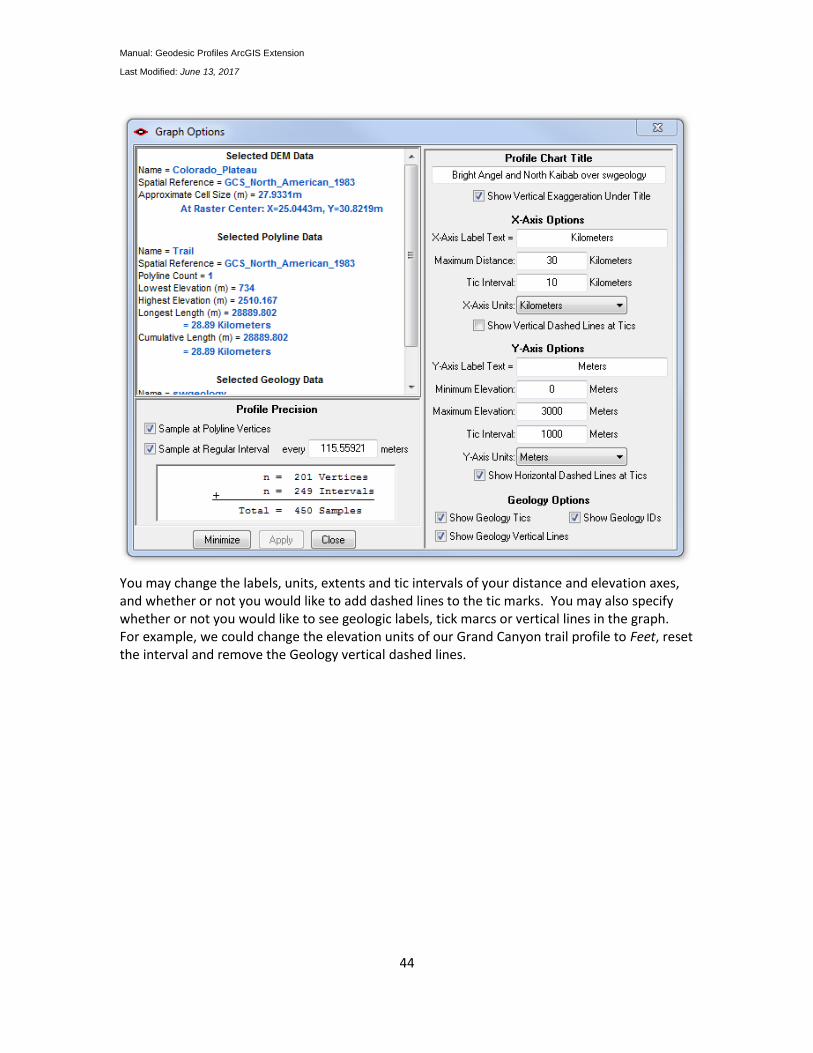
You may change the labels, units, extents and tic intervals of your distance and elevation axes, and whether or not you would like to add dashed lines to the tic marks. You may also specify whether or not you would like to see geologic labels, tick marcs or vertical lines in the graph. For example, we could change the elevation units of our Grand Canyon trail profile to Feet, reset the interval and remove the Geology vertical dashed lines.
Manual: Geodesic Profiles ArcGIS Extension
Last Modified: June 13, 2017
45
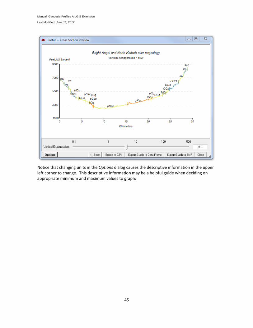
Notice that changing units in the Options dialog causes the descriptive information in the upper left corner to change. This descriptive information may be a helpful guide when deciding on appropriate minimum and maximum values to graph:
Manual: Geodesic Profiles ArcGIS Extension
Last Modified: June 13, 2017
46
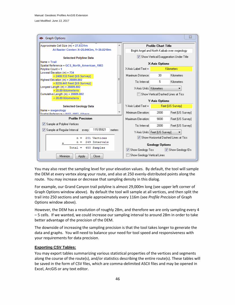
You may also reset the sampling level for your elevation values. By default, the tool will sample the DEM at every vertex along your route, and also at 250 evenly-distributed points along the route. You may increase or decrease that sampling density in this dialog.
For example, our Grand Canyon trail polyline is almost 29,000m long (see upper left corner of Graph Options window above). By default the tool will sample at all vertices, and then split the trail into 250 sections and sample approximately every 116m (see Profile Precision of Graph Options window above).
However, the DEM has a resolution of roughly 28m, and therefore we are only sampling every 4 – 5 cells. If we wanted, we could increase our sampling interval to around 28m in order to take better advantage of the precision of the DEM.
The downside of increasing the sampling precision is that the tool takes longer to generate the data and graphs. You will need to balance your need for tool speed and responsiveness with your requirements for data precision.
Exporting CSV Tables:
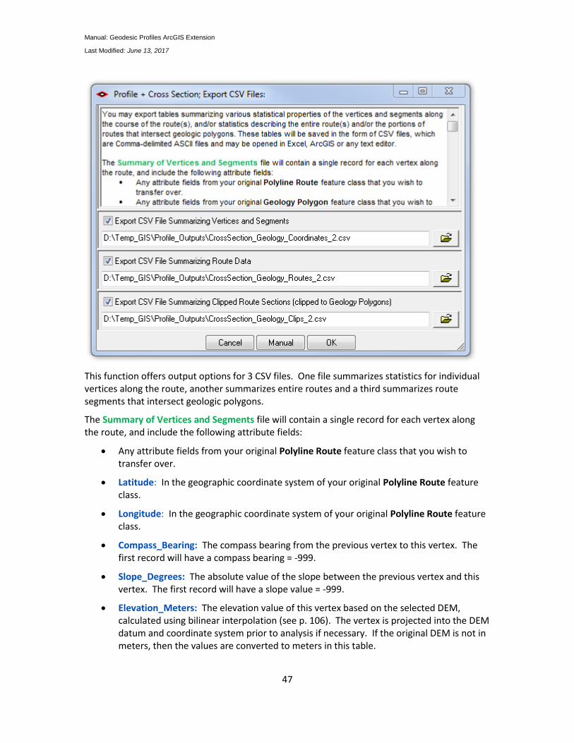
You may export tables summarizing various statistical properties of the vertices and segments along the course of the route(s), and/or statistics describing the entire route(s). These tables will be saved in the form of CSV files, which are comma-delimited ASCII files and may be opened in Excel, ArcGIS or any text editor.
Manual: Geodesic Profiles ArcGIS Extension
Last Modified: June 13, 2017
47
This function offers output options for 3 CSV files. One file summarizes statistics for individual vertices along the route, another summarizes entire routes and a third summarizes route segments that intersect geologic polygons.
The Summary of Vertices and Segments file will contain a single record for each vertex along the route, and include the following attribute fields:
Any attribute fields from your original Polyline Route feature class that you wish to transfer over.
Latitude: In the geographic coordinate system of your original Polyline Route feature class.
Longitude: In the geographic coordinate system of your original Polyline Route feature class.
Compass_Bearing: The compass bearing from the previous vertex to this vertex. The first record will have a compass bearing = -999.
Slope_Degrees: The absolute value of the slope between the previous vertex and this vertex. The first record will have a slope value = -999.
Elevation_Meters: The elevation value of this vertex based on the selected DEM, calculated using bilinear interpolation (see p. 106). The vertex is projected into the DEM datum and coordinate system prior to analysis if necessary. If the original DEM is not in meters, then the values are converted to meters in this table.
Manual: Geodesic Profiles ArcGIS Extension
Last Modified: June 13, 2017
48
Segment_Geodesic_Distance_Meters: The distance, in meters, between the previous vertex and this one, calculated using Vincenty's algorithms to estimate geodesic distances over the original Polygon Route feature class spheroid (see Vincenty 1975; also p. 124 of this manual).
Segment_Surface_Distance_Meters: The surface distance, in meters, between the previous vertex and this one, calculated using the Pythagorean theorem to determine the hypotenuse of the triangle formed by the change in elevation and the geodesic distance.
Cumulative_Proportion: The proportion of the original route at this vertex. This proportion is based on the surface distance of the line, not the geodesic distance.
Cumulative_Geodesic_Distance_Meters: The total geodesic distance along the route up to this vertex.
Cumulative_Surface_Distance_Meters: The total surface distance along the route up to this vertex.
X_Original_Units: The X-coordinate in the original units of the source Polyline Route feature class. For example, if the source data were in UTM coordinates, then this value would be the vertex Easting value.
Y_Original_Units: The Y-coordinate in the original units of the source Polyline Route feature class. For example, if the source data were in UTM coordinates, then this value would be the vertex Northing value.
Elevation_Original_Units: The elevation value in the original units of the source DEM.
Exaggeration_Factor: The exaggeration factor used to adjust the dimensions of the profile graph. This may be useful if you wish to generate a profile graph from these points in some other software package such as R.
Exaggerated_Elev: The elevation of the vertex after being multiplied by the exaggeration factor. This is the value that is actually being plotted on the graph, and this value may also be useful if you wish to generate a profile graph from these points in some other software package.
The Summary of Routes file will contain a single record for each route analyzed, and will include the following attribute fields:
Any attribute fields from your original Polyline Route feature class that you wish to transfer over.
Sample_Points: The number of DEM values sampled to generate the statistics for this polyline.
Start_Latitude: In the geographic coordinate system of your original Polyline Route feature class.
Start_Longitude: In the geographic coordinate system of your original Polyline Route feature class.
Manual: Geodesic Profiles ArcGIS Extension
Last Modified: June 13, 2017
49
End_Latitude: In the geographic coordinate system of your original Polyline Route feature class.
End_Longitude: In the geographic coordinate system of your original Polyline Route feature class.
Start_Elevation: The elevation value of starting point based on the selected DEM, calculated using bilinear interpolation (see p. 106). The vertex is projected into the DEM datum and coordinate system prior to analysis if necessary. If the original DEM is not in meters, then the values are converted to meters in this table.
End_Elevation: The elevation of the ending point based on the selected DEM.
Min_Elevation: The elevation of the lowest point based on the selected DEM.
Max_Elevation: The elevation of the highest point based on the selected DEM.
Avg_Slope: The average slope over the course of the route, calculated as the weighted mean of the segment slopes, weighted by the segment surface distances.
Slope_StDev: The standard deviation of slope over the course of the route.
Avg_Bearing: The mean direction of the route, equal to the bearing from the starting point to the ending point of the route (see p. 137 for details).
BearingMRL: The Mean Resultant Length of the route, calculated as the ratio of the geodesic length of the complete route divided by the geodesic distance of the straight line between the starting and ending points (see p. 137 for details). The MRL is the basis of several circular measures of dispersion (see Batschelet 1981, Fisher 1995, Mardia and Jupp 2000). MRL values near 1 indicate little direction variation over the line.
Length_Geodesic: The geodesic length of the route.
Length_Surface: The surface length of the route.
Surface Ratio: The ratio of [Surface Length] / [Geodesic Length]. Values near 1 indicate a flat line, while values > 1 indicate increasing elevational variation.
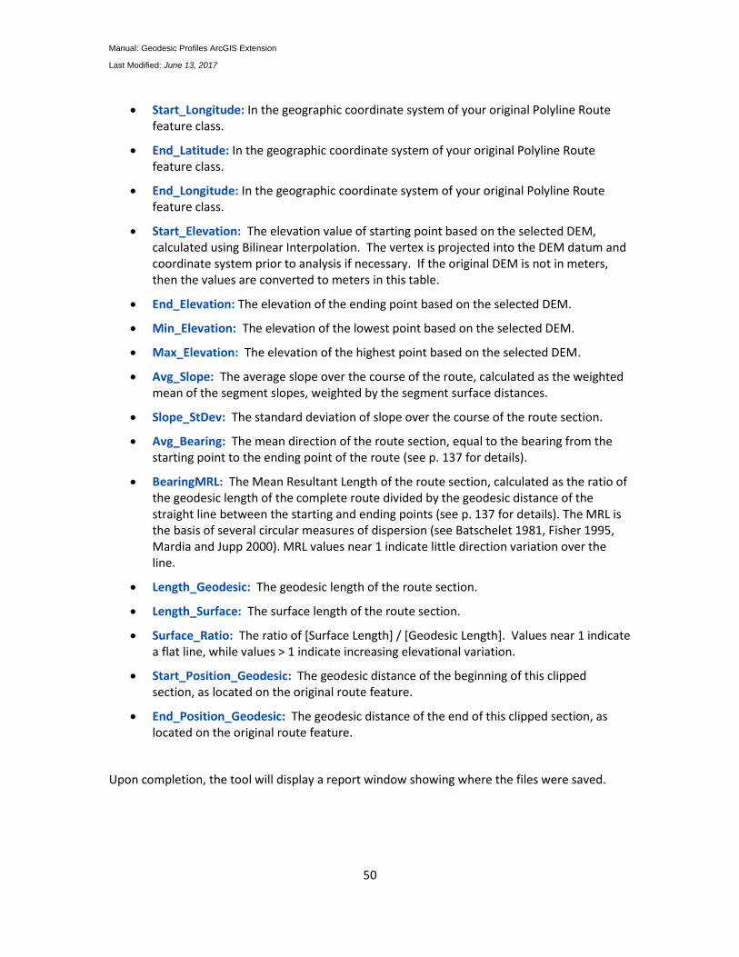
The Summary of Clips file will contain a single record for each section of the route polyline clipped within each intersecting geology polygon, and will include the following attribute fields:
Any attribute fields from your original Polyline Route feature class that you wish to transfer over.
Any attribute fields from your original Geology Polygon feature class that you wish to transfer over.
Sample_Points: The number of DEM values sampled to generate the statistics for this polyline section.
Start_Latitude: In the geographic coordinate system of your original Polyline Route feature class.
Manual: Geodesic Profiles ArcGIS Extension
Last Modified: June 13, 2017
50
Start_Longitude: In the geographic coordinate system of your original Polyline Route feature class.
End_Latitude: In the geographic coordinate system of your original Polyline Route feature class.
End_Longitude: In the geographic coordinate system of your original Polyline Route feature class.
Start_Elevation: The elevation value of starting point based on the selected DEM, calculated using Bilinear Interpolation. The vertex is projected into the DEM datum and coordinate system prior to analysis if necessary. If the original DEM is not in meters, then the values are converted to meters in this table.
End_Elevation: The elevation of the ending point based on the selected DEM.
Min_Elevation: The elevation of the lowest point based on the selected DEM.
Max_Elevation: The elevation of the highest point based on the selected DEM.
Avg_Slope: The average slope over the course of the route, calculated as the weighted mean of the segment slopes, weighted by the segment surface distances.
Slope_StDev: The standard deviation of slope over the course of the route section.
Avg_Bearing: The mean direction of the route section, equal to the bearing from the starting point to the ending point of the route (see p. 137 for details).
BearingMRL: The Mean Resultant Length of the route section, calculated as the ratio of the geodesic length of the complete route divided by the geodesic distance of the straight line between the starting and ending points (see p. 137 for details). The MRL is the basis of several circular measures of dispersion (see Batschelet 1981, Fisher 1995, Mardia and Jupp 2000). MRL values near 1 indicate little direction variation over the line.
Length_Geodesic: The geodesic length of the route section.
Length_Surface: The surface length of the route section.
Surface_Ratio: The ratio of [Surface Length] / [Geodesic Length]. Values near 1 indicate a flat line, while values > 1 indicate increasing elevational variation.
Start_Position_Geodesic: The geodesic distance of the beginning of this clipped section, as located on the original route feature.
End_Position_Geodesic: The geodesic distance of the end of this clipped section, as located on the original route feature.
Upon completion, the tool will display a report window showing where the files were saved.
Manual: Geodesic Profiles ArcGIS Extension
Last Modified: June 13, 2017
51
Manual: Geodesic Profiles ArcGIS Extension
Last Modified: June 13, 2017
52
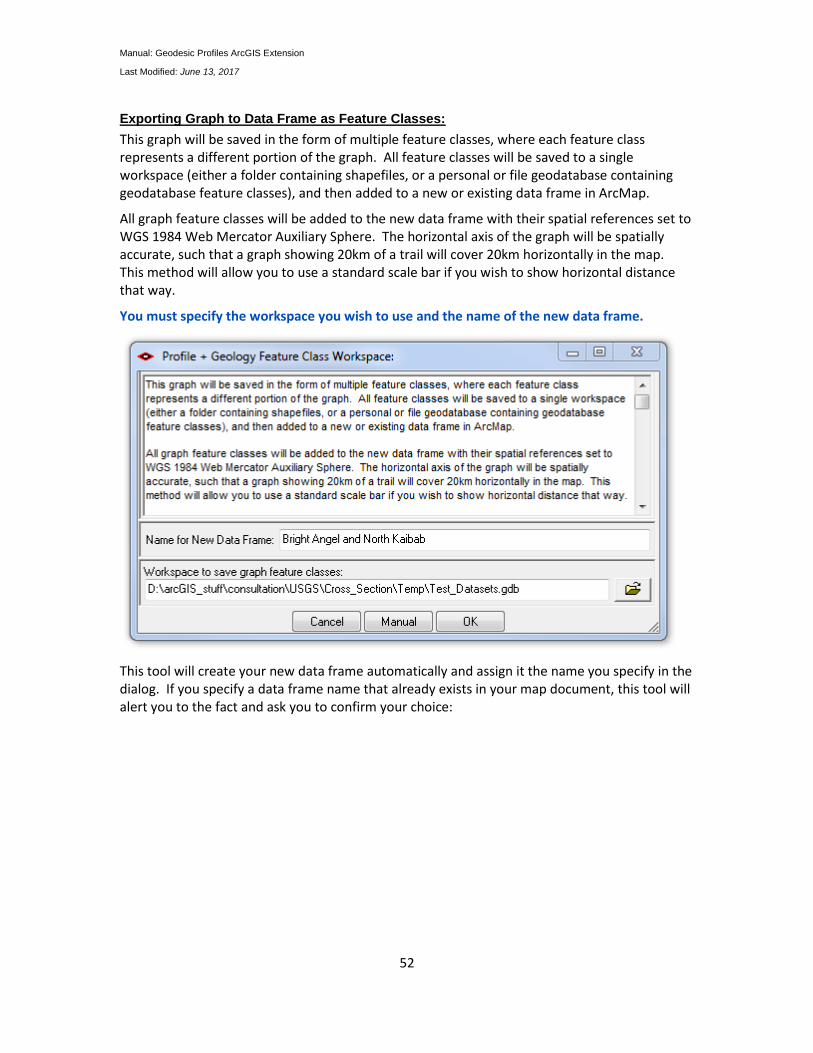
Exporting Graph to Data Frame as Feature Classes:
This graph will be saved in the form of multiple feature classes, where each feature class represents a different portion of the graph. All feature classes will be saved to a single workspace (either a folder containing shapefiles, or a personal or file geodatabase containing geodatabase feature classes), and then added to a new or existing data frame in ArcMap.
All graph feature classes will be added to the new data frame with their spatial references set to WGS 1984 Web Mercator Auxiliary Sphere. The horizontal axis of the graph will be spatially accurate, such that a graph showing 20km of a trail will cover 20km horizontally in the map. This method will allow you to use a standard scale bar if you wish to show horizontal distance that way.
You must specify the workspace you wish to use and the name of the new data frame.
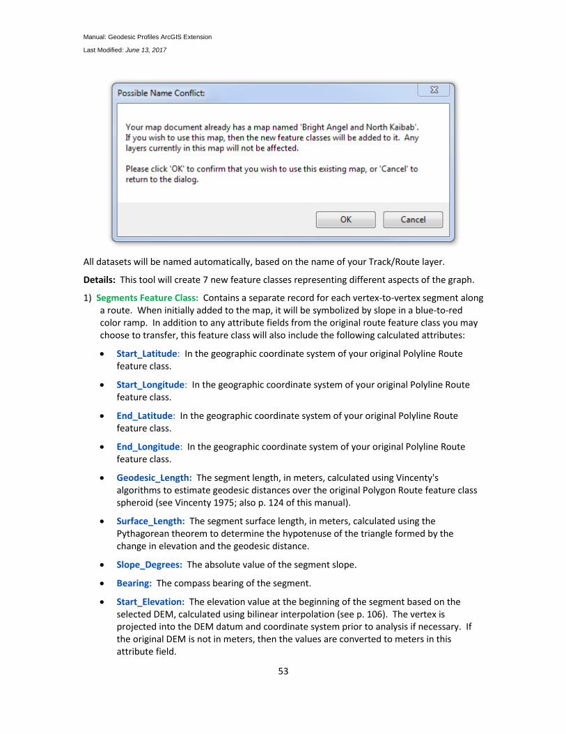
This tool will create your new data frame automatically and assign it the name you specify in the dialog. If you specify a data frame name that already exists in your map document, this tool will alert you to the fact and ask you to confirm your choice:
Manual: Geodesic Profiles ArcGIS Extension
Last Modified: June 13, 2017
53
All datasets will be named automatically, based on the name of your Track/Route layer.
Details: This tool will create 7 new feature classes representing different aspects of the graph.
1) Segments Feature Class: Contains a separate record for each vertex-to-vertex segment along a route. When initially added to the map, it will be symbolized by slope in a blue-to-red color ramp. In addition to any attribute fields from the original route feature class you may choose to transfer, this feature class will also include the following calculated attributes:
Start_Latitude: In the geographic coordinate system of your original Polyline Route feature class.
Start_Longitude: In the geographic coordinate system of your original Polyline Route feature class.
End_Latitude: In the geographic coordinate system of your original Polyline Route feature class.
End_Longitude: In the geographic coordinate system of your original Polyline Route feature class.
Geodesic_Length: The segment length, in meters, calculated using Vincenty's algorithms to estimate geodesic distances over the original Polygon Route feature class spheroid (see Vincenty 1975; also p. 124 of this manual).
Surface_Length: The segment surface length, in meters, calculated using the Pythagorean theorem to determine the hypotenuse of the triangle formed by the change in elevation and the geodesic distance.
Slope_Degrees: The absolute value of the segment slope.
Bearing: The compass bearing of the segment.
Start_Elevation: The elevation value at the beginning of the segment based on the selected DEM, calculated using bilinear interpolation (see p. 106). The vertex is projected into the DEM datum and coordinate system prior to analysis if necessary. If the original DEM is not in meters, then the values are converted to meters in this attribute field.
Manual: Geodesic Profiles ArcGIS Extension
Last Modified: June 13, 2017
54
Mid_Elevation: The elevation value at the centerpoint of the segment.
End_Elevation: The elevation value at the end of the segment.
End_Proportion: The proportion of the original route at the segment endpoint. This proportion is based on the surface distance of the line, not the geodesic distance. Values will range from 0 to 1.
Total_Geodesic_Distance: The total geodesic distance, in meters, along the route up to the end of this segment.
Total_Surface_Distance: The total surface distance, in meters, along the route up to the end of this segment.
2) Polyline Feature Class: Contains a separate record for each route showing the profile of the route over the DEM. When initially added to the map, it will be symbolized by ID value based on the ID field you select. If you do not select an ID field, it will be symbolized by the Feature Object ID of the original route. In addition to any attribute fields from the original route feature class you may choose to transfer, this feature class will also include the following calculated attributes:
Sample_Points: The number of DEM values sampled to generate the statistics for this polyline.
Start_Latitude: In the geographic coordinate system of your original Polyline Route feature class.
Start_Longitude: In the geographic coordinate system of your original Polyline Route feature class.
End_Latitude: In the geographic coordinate system of your original Polyline Route feature class.
End_Longitude: In the geographic coordinate system of your original Polyline Route feature class.
Start_Elevation: The elevation value of starting point based on the selected DEM, calculated using bilinear interpolation (see p. 106). The vertex is projected into the DEM datum and coordinate system prior to analysis if necessary. If the original DEM is not in meters, then the values are converted to meters in this table.
End_Elevation: The elevation of the ending point based on the selected DEM.
Min_Elevation: The elevation of the lowest point based on the selected DEM.
Max_Elevation: The elevation of the highest point based on the selected DEM.
Avg_Slope: The average slope over the course of the route, calculated as the weighted mean of the segment slopes, weighted by the segment surface distances.
Slope_StDev: The standard deviation of slope over the course of the route.
Avg_Bearing: The mean direction of the route, equal to the bearing from the starting point to the ending point of the route.
Manual: Geodesic Profiles ArcGIS Extension
Last Modified: June 13, 2017
55
BearingMRL: The Mean Resultant Length of the route, calculated as the ratio of the geodesic length of the complete route divided by the geodesic distance of the straight line between the starting and ending points. The MRL is the basis of several circular measures of dispersion (see Batschelet 1981, Fisher 1995, Mardia and Jupp 2000). MRL values near 1 indicate little direction variation over the line.
Length_Geodesic: The geodesic length of the route.
Length_Surface: The surface length of the route.
Surface Ratio: The ratio of [Surface Length] / [Geodesic Length]. Values near 1 indicate a flat line, while values > 1 indicate increasing elevational variation.
3) Polygon Feature Class: Similar to the Polyline Feature Class, except that it symbolizes the route using a polygon to symbolize the portion of the graph underneath the route profile. Contains a separate record for each route. When initially added to the map, it will be symbolized by ID value based on the ID field you select. If you do not select an ID field, it will be symbolized by the Feature Object ID of the original route. This feature class will contain exactly the same attribute fields and values as the Polyline Feature Class described above.
4) Clipped Polyline Feature Class: Contains a separate record for each intersection between the route and a geology polygon, showing the profile of the route over the DEM. When initially added to the map, it will be symbolized by the color of the Geology polygons. In addition to any attribute fields from the original route and geology feature classes you may choose to transfer, this feature class will also include the following calculated attributes:
Sample_Points: The number of DEM values sampled to generate the statistics for this clipped portion of the route polyline.
Start_Latitude: In the geographic coordinate system of your original Polyline Route feature class.
Start_Longitude: In the geographic coordinate system of your original Polyline Route feature class.
End_Latitude: In the geographic coordinate system of your original Polyline Route feature class.
End_Longitude: In the geographic coordinate system of your original Polyline Route feature class.
Start_Elevation: The elevation value of starting point based on the selected DEM, calculated using Bilinear Interpolation. The vertex is projected into the DEM datum and coordinate system prior to analysis if necessary. If the original DEM is not in meters, then the values are converted to meters in this table.
End_Elevation: The elevation of the ending point based on the selected DEM.
Min_Elevation: The elevation of the lowest point based on the selected DEM.
Max_Elevation: The elevation of the highest point based on the selected DEM.
Avg_Slope: The average slope over the course of the route, calculated as the weighted mean of the segment slopes, weighted by the segment surface distances.
Manual: Geodesic Profiles ArcGIS Extension
Last Modified: June 13, 2017
56
Slope_StDev: The standard deviation of slope over the course of the route.
Avg_Bearing: The mean direction of the route, equal to the bearing from the starting point to the ending point of the route.
BearingMRL: The Mean Resultant Length of the route, calculated as the ratio of the geodesic length of the complete route divided by the geodesic distance of the straight line between the starting and ending points. The MRL is the basis of several circular measures of dispersion (see Batschelet 1981, Fisher 1995, Mardia and Jupp 2000). MRL values near 1 indicate little direction variation over the line.
Length_Geodesic: The geodesic length of the route.
Length_Surface: The surface length of the route.
Surface_Ratio: The ratio of [Surface Length] / [Geodesic Length]. Values near 1 indicate a flat line, while values > 1 indicate increasing elevational variation.
Start_Position_Geodesic: The geodesic distance of the beginning of this clipped section, as located on the original route feature.
End_Position_Geodesic: The geodesic distance of the end of this clipped section, as located on the original route feature.
5) Clipped Polyline Tic Mark Feature Class: Contains a separate record for the intersection points between the route and geology polygons, showing a short vertical line that intersects the profile line. This feature class is intended primarily to add aesthetic qualities to the profile graph. When initially added to the map, it will be symbolized by the color of the Geology polygons. This feature class will only include the following calculated attributes:
Left_GeoID: The geology polygon ID value on the left side of the tick mark.
Right_GeoID: The geology polygon ID value on the right side of the tick mark.
Label_Value: A string value composed of [Left_GeoID] + a vertical line ("|") + [Right_GeoID]. This might be useful for labeling purposes in the graph.
Position_Geodesic: The geodesic distance of this point, as located on the original route feature.
Elevation: The elevation, in meters, at this point.
Latitude: In the geographic coordinate system of your original Polyline Route feature class.
Longitude: In the geographic coordinate system of your original Polyline Route feature class.
6) Clipped Polyline Vertical Line Feature Class: Contains a separate record for the intersection points between the route and geology polygons, showing a vertical line that extends from the bottom of the graph up to the profile line. This feature class is intended primarily to add aesthetic qualities to the profile graph. When initially added to the map, it will be symbolized
Manual: Geodesic Profiles ArcGIS Extension
Last Modified: June 13, 2017
57
by the color of the Geology polygons. This feature class will only include the following calculated attributes:
Left_GeoID: The geology polygon ID value on the left side of the line.
Right_GeoID: The geology polygon ID value on the right side of the line.
Label_Value: A string value composed of [Left_GeoID] + a vertical line ("|") + [Right_GeoID]. This might be useful for labeling purposes in the graph.
Position_Geodesic: The geodesic distance of this point, as located on the original route feature.
Elevation: The elevation, in meters, at this point.
Latitude: In the geographic coordinate system of your original Polyline Route feature class.
Longitude: In the geographic coordinate system of your original Polyline Route feature class.
7) Graph_Lines: Simply shows the reference lines of the graph, including axes, tick marks and horizontal/vertical references. Attribute values include the name of the line (X-Axis, Y-Axis, X-Tic, Y-Tic, X-Reference and Y-Reference), and a label value for that line.
This tool will also add graphic text boxes for label values, axis names and the chart title. Note: These graphics can be converted to annotation by right-clicking data frame name and choosing "Convert Labels to Annotation". This option helps the labels look better if you add the graph to a layout. See also a known issue with exported graphic text on p. 96.
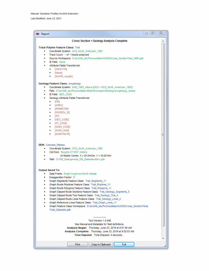
Upon completion, the tool will show you a report detailing what it did:
Manual: Geodesic Profiles ArcGIS Extension
Last Modified: June 13, 2017
58
Manual: Geodesic Profiles ArcGIS Extension
Last Modified: June 13, 2017
59
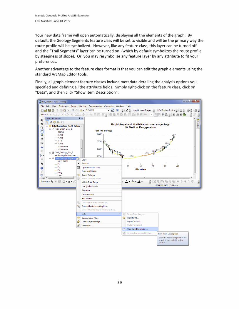
Your new data frame will open automatically, displaying all the elements of the graph. By default, the Geology Segments feature class will be set to visible and will be the primary way the route profile will be symbolized. However, like any feature class, this layer can be turned off and the “Trail Segments” layer can be turned on. (which by default symbolizes the route profile by steepness of slope). Or, you may resymbolize any feature layer by any attribute to fit your preferences.
Another advantage to the feature class format is that you can edit the graph elements using the standard ArcMap Editor tools.
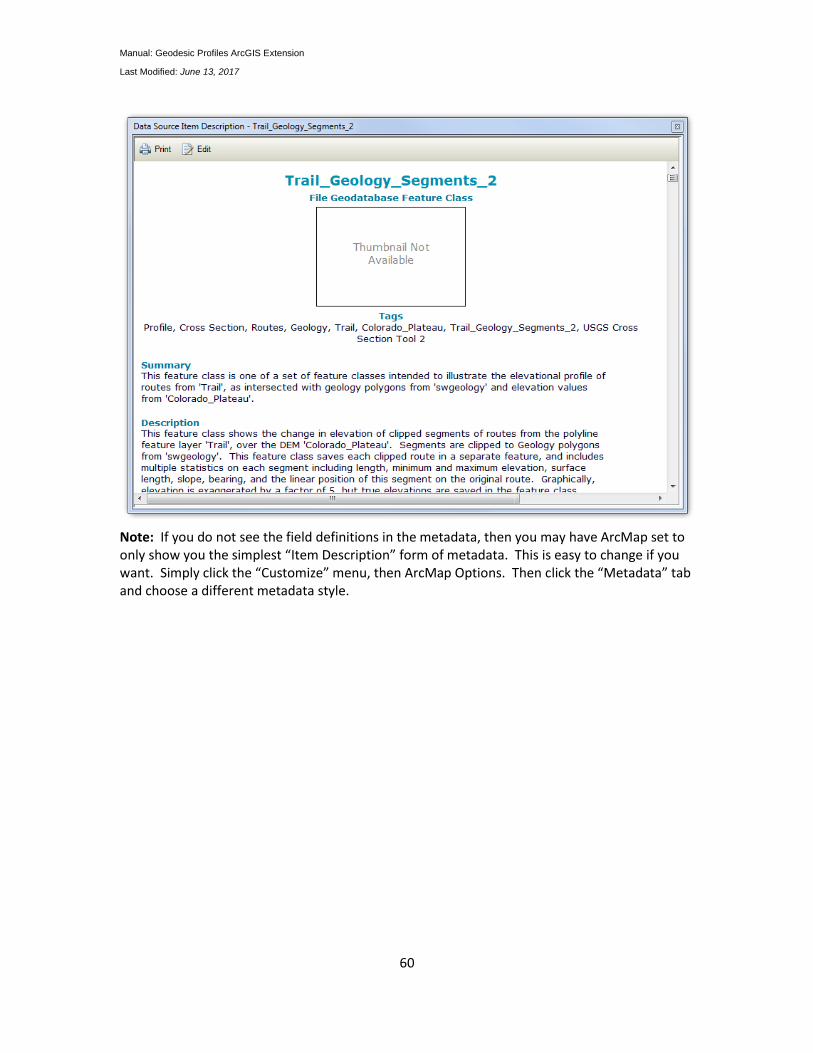
Finally, all graph element feature classes include metadata detailing the analysis options you specified and defining all the attribute fields. Simply right-click on the feature class, click on “Data”, and then click “Show Item Description”:
Manual: Geodesic Profiles ArcGIS Extension
Last Modified: June 13, 2017
60
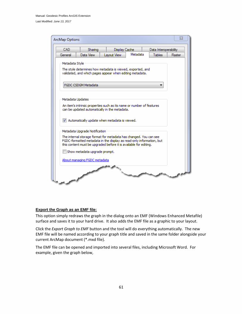
Note: If you do not see the field definitions in the metadata, then you may have ArcMap set to only show you the simplest “Item Description” form of metadata. This is easy to change if you want. Simply click the “Customize” menu, then ArcMap Options. Then click the “Metadata” tab and choose a different metadata style.
Manual: Geodesic Profiles ArcGIS Extension
Last Modified: June 13, 2017
61
Export the Graph as an EMF file:
This option simply redraws the graph in the dialog onto an EMF (Windows Enhanced Metafile) surface and saves it to your hard drive. It also adds the EMF file as a graphic to your layout.
Click the Export Graph to EMF button and the tool will do everything automatically. The new EMF file will be named according to your graph title and saved in the same folder alongside your current ArcMap document (*.mxd file).
The EMF file can be opened and imported into several files, including Microsoft Word. For example, given the graph below,
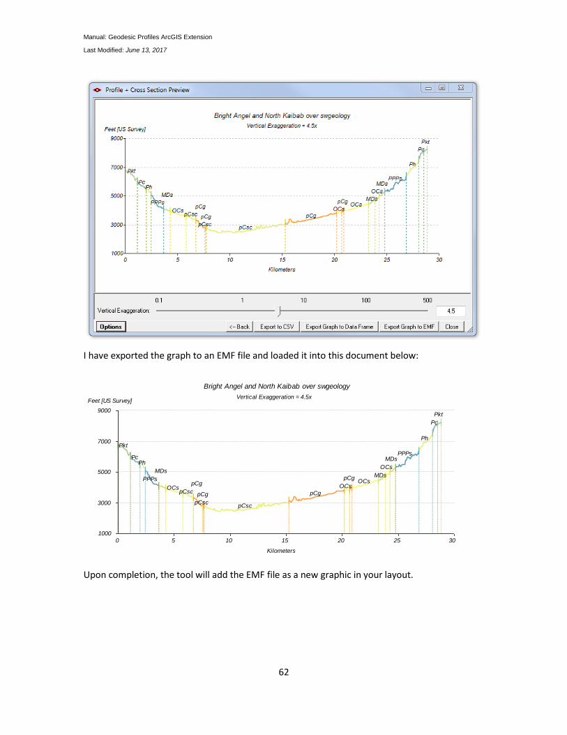
Manual: Geodesic Profiles ArcGIS Extension
Last Modified: June 13, 2017
62
I have exported the graph to an EMF file and loaded it into this document below:
Upon completion, the tool will add the EMF file as a new graphic in your layout.
1000
0
9000
3000
5000
7000
Feet [US Survey]
305 10 15 20 25
Kilometers
Vertical Exaggeration = 4.5x
Pkt
PcPh
PPPs
MDs
OCspCsc
pCg
pCsc
pCg
pCsc
pCg
OCs
pCgOCs
MDs
OCs
MDsPPPs
Ph
Pc
Pkt
Bright Angel and North Kaibab over swgeology
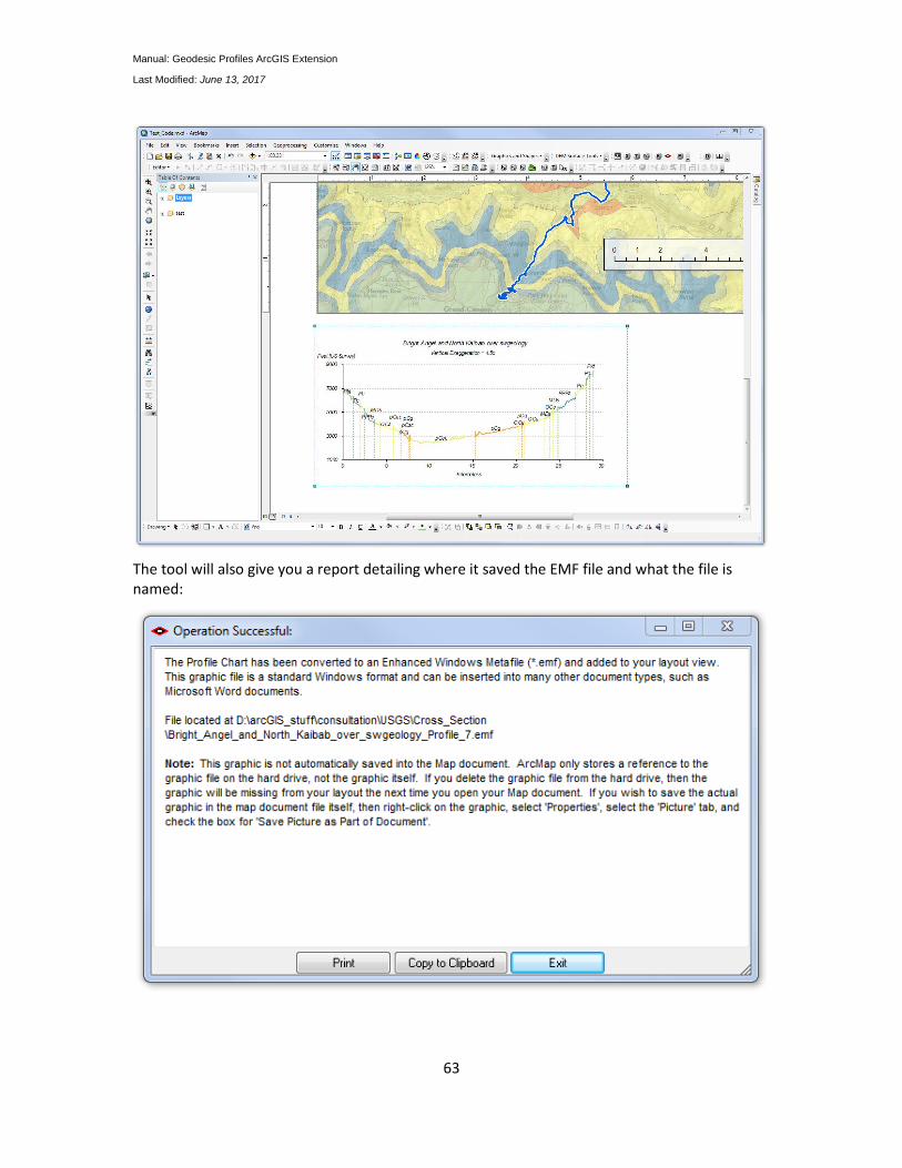
Manual: Geodesic Profiles ArcGIS Extension
Last Modified: June 13, 2017
63
The tool will also give you a report detailing where it saved the EMF file and what the file is named:
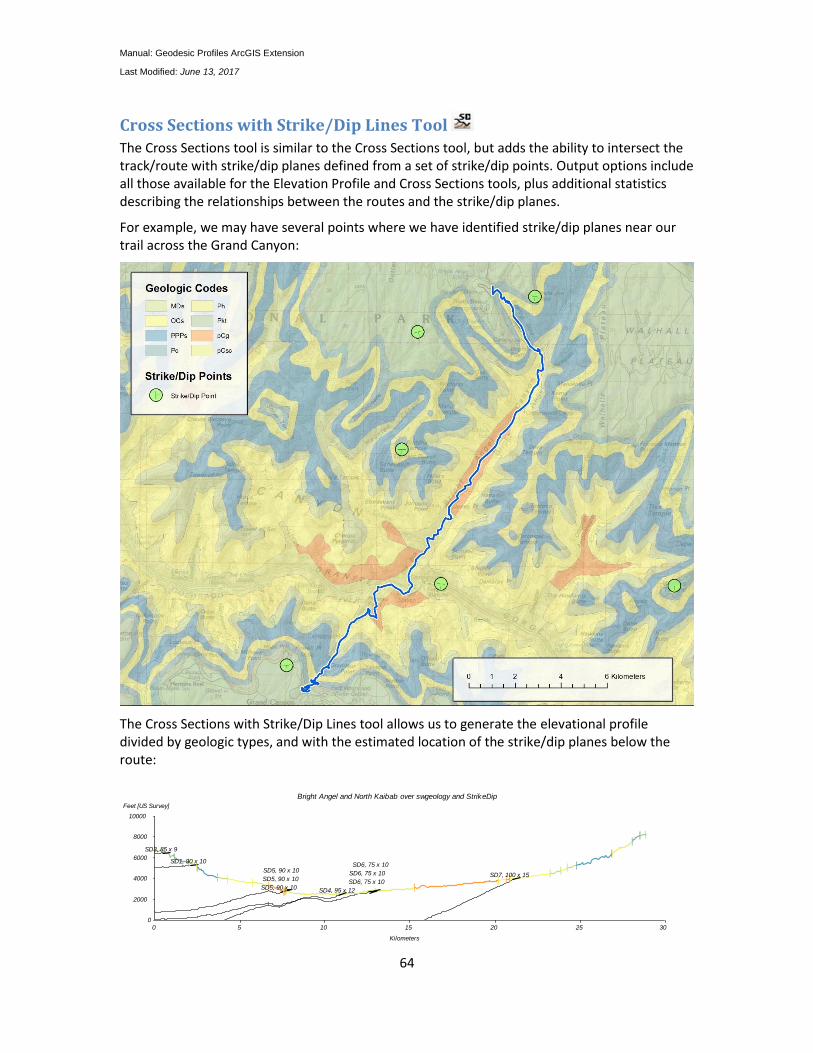
Manual: Geodesic Profiles ArcGIS Extension
Last Modified: June 13, 2017
64
Cross Sections with Strike/Dip Lines Tool
The Cross Sections tool is similar to the Cross Sections tool, but adds the ability to intersect the track/route with strike/dip planes defined from a set of strike/dip points. Output options include all those available for the Elevation Profile and Cross Sections tools, plus additional statistics describing the relationships between the routes and the strike/dip planes.
For example, we may have several points where we have identified strike/dip planes near our trail across the Grand Canyon:
The Cross Sections with Strike/Dip Lines tool allows us to generate the elevational profile divided by geologic types, and with the estimated location of the strike/dip planes below the route:
0
0
10000
2000
4000
6000
8000
Feet [US Survey]
305 10 15 20 25
Kilometers
SD1, 90 x 10
SD3, 85 x 9
SD4, 95 x 12SD5, 90 x 10
SD5, 90 x 10
SD5, 90 x 10
SD6, 75 x 10
SD6, 75 x 10
SD6, 75 x 10
SD7, 100 x 15
Bright Angel and North Kaibab over swgeology and StrikeDip
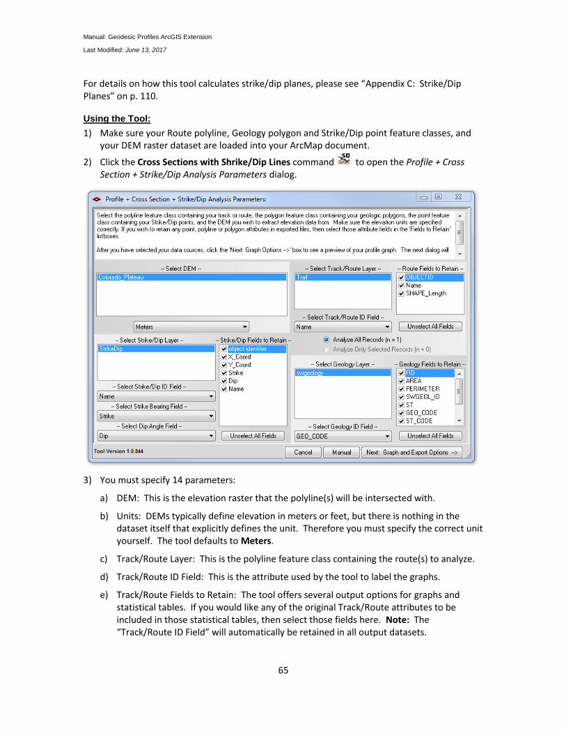
Manual: Geodesic Profiles ArcGIS Extension
Last Modified: June 13, 2017
65
For details on how this tool calculates strike/dip planes, please see “Appendix C: Strike/Dip Planes” on p. 110.
Using the Tool:
1) Make sure your Route polyline, Geology polygon and Strike/Dip point feature classes, and your DEM raster dataset are loaded into your ArcMap document.
2) Click the Cross Sections with Shrike/Dip Lines command to open the Profile + Cross Section + Strike/Dip Analysis Parameters dialog.
3) You must specify 14 parameters:
a) DEM: This is the elevation raster that the polyline(s) will be intersected with.
b) Units: DEMs typically define elevation in meters or feet, but there is nothing in the dataset itself that explicitly defines the unit. Therefore you must specify the correct unit yourself. The tool defaults to Meters.
c) Track/Route Layer: This is the polyline feature class containing the route(s) to analyze.
d) Track/Route ID Field: This is the attribute used by the tool to label the graphs.
e) Track/Route Fields to Retain: The tool offers several output options for graphs and statistical tables. If you would like any of the original Track/Route attributes to be included in those statistical tables, then select those fields here. Note: The “Track/Route ID Field” will automatically be retained in all output datasets.
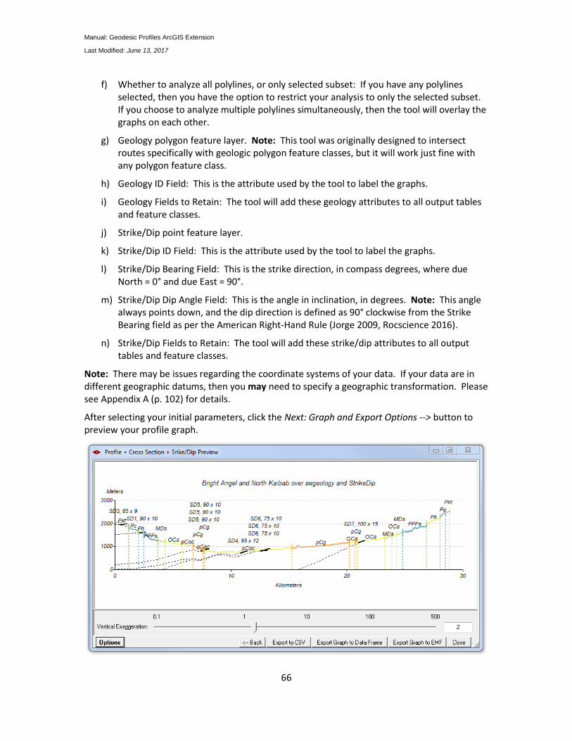
Manual: Geodesic Profiles ArcGIS Extension
Last Modified: June 13, 2017
66
f) Whether to analyze all polylines, or only selected subset: If you have any polylines selected, then you have the option to restrict your analysis to only the selected subset. If you choose to analyze multiple polylines simultaneously, then the tool will overlay the graphs on each other.
g) Geology polygon feature layer. Note: This tool was originally designed to intersect routes specifically with geologic polygon feature classes, but it will work just fine with any polygon feature class.
h) Geology ID Field: This is the attribute used by the tool to label the graphs.
i) Geology Fields to Retain: The tool will add these geology attributes to all output tables and feature classes.
j) Strike/Dip point feature layer.
k) Strike/Dip ID Field: This is the attribute used by the tool to label the graphs.
l) Strike/Dip Bearing Field: This is the strike direction, in compass degrees, where due North = 0° and due East = 90°.
m) Strike/Dip Dip Angle Field: This is the angle in inclination, in degrees. Note: This angle always points down, and the dip direction is defined as 90° clockwise from the Strike Bearing field as per the American Right-Hand Rule (Jorge 2009, Rocscience 2016).
n) Strike/Dip Fields to Retain: The tool will add these strike/dip attributes to all output tables and feature classes.
Note: There may be issues regarding the coordinate systems of your data. If your data are in different geographic datums, then you may need to specify a geographic transformation. Please see Appendix A (p. 102) for details.
After selecting your initial parameters, click the Next: Graph and Export Options --> button to preview your profile graph.
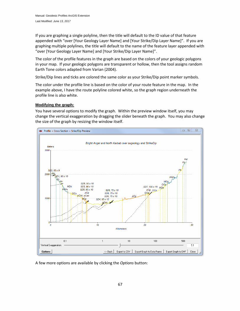
Manual: Geodesic Profiles ArcGIS Extension
Last Modified: June 13, 2017
67
If you are graphing a single polyline, then the title will default to the ID value of that feature appended with “over [Your Geology Layer Name] and [Your Strike/Dip Layer Name]”. If you are graphing multiple polylines, the title will default to the name of the feature layer appended with “over [Your Geology Layer Name] and [Your Strike/Dip Layer Name]”.
The color of the profile features in the graph are based on the colors of your geologic polygons in your map. If your geologic polygons are transparent or hollow, then the tool assigns random Earth Tone colors adapted from Varian (2004).
Strike/Dip lines and ticks are colored the same color as your Strike/Dip point marker symbols.
The color under the profile line is based on the color of your route feature in the map. In the example above, I have the route polyline colored white, so the graph region underneath the profile line is also white.
Modifying the graph:
You have several options to modify the graph. Within the preview window itself, you may change the vertical exaggeration by dragging the slider beneath the graph. You may also change the size of the graph by resizing the window itself.
A few more options are available by clicking the Options button:
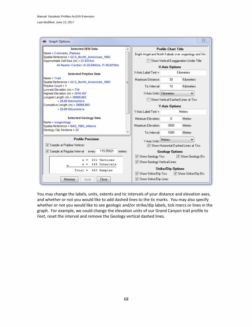
Manual: Geodesic Profiles ArcGIS Extension
Last Modified: June 13, 2017
68
You may change the labels, units, extents and tic intervals of your distance and elevation axes, and whether or not you would like to add dashed lines to the tic marks. You may also specify whether or not you would like to see geologic and/or strike/dip labels, tick marcs or lines in the graph. For example, we could change the elevation units of our Grand Canyon trail profile to Feet, reset the interval and remove the Geology vertical dashed lines.
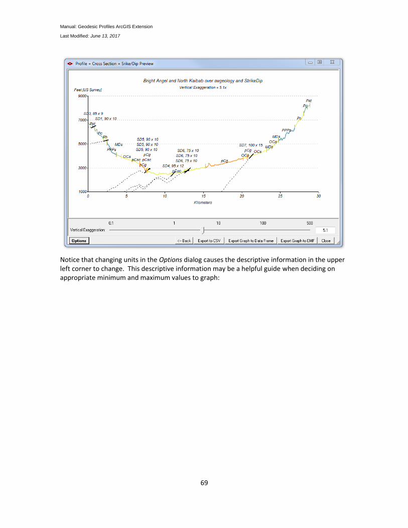
Manual: Geodesic Profiles ArcGIS Extension
Last Modified: June 13, 2017
69
Notice that changing units in the Options dialog causes the descriptive information in the upper left corner to change. This descriptive information may be a helpful guide when deciding on appropriate minimum and maximum values to graph:
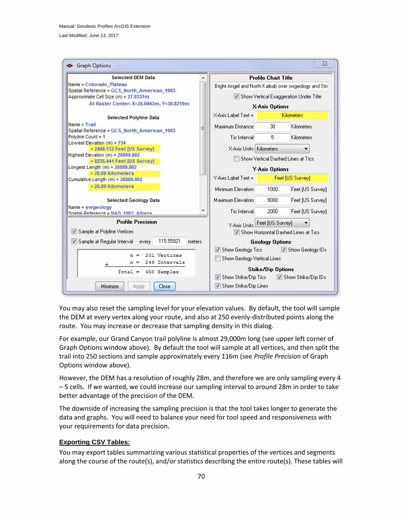
Manual: Geodesic Profiles ArcGIS Extension
Last Modified: June 13, 2017
70
You may also reset the sampling level for your elevation values. By default, the tool will sample the DEM at every vertex along your route, and also at 250 evenly-distributed points along the route. You may increase or decrease that sampling density in this dialog.
For example, our Grand Canyon trail polyline is almost 29,000m long (see upper left corner of Graph Options window above). By default the tool will sample at all vertices, and then split the trail into 250 sections and sample approximately every 116m (see Profile Precision of Graph Options window above).
However, the DEM has a resolution of roughly 28m, and therefore we are only sampling every 4 – 5 cells. If we wanted, we could increase our sampling interval to around 28m in order to take better advantage of the precision of the DEM.
The downside of increasing the sampling precision is that the tool takes longer to generate the data and graphs. You will need to balance your need for tool speed and responsiveness with your requirements for data precision.
Exporting CSV Tables:
You may export tables summarizing various statistical properties of the vertices and segments along the course of the route(s), and/or statistics describing the entire route(s). These tables will
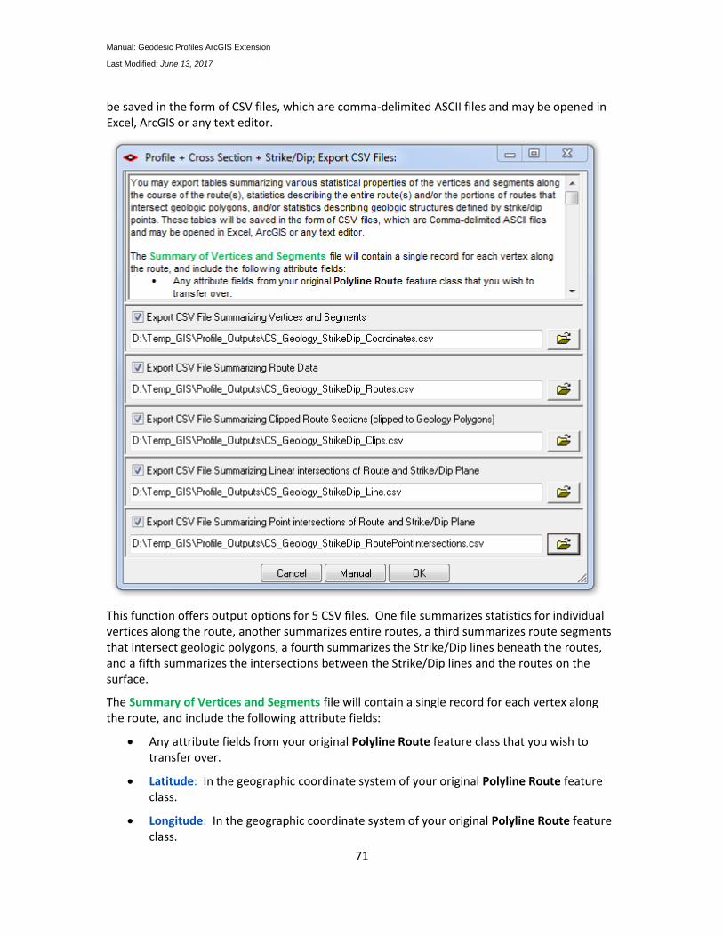
Manual: Geodesic Profiles ArcGIS Extension
Last Modified: June 13, 2017
71
be saved in the form of CSV files, which are comma-delimited ASCII files and may be opened in Excel, ArcGIS or any text editor.
This function offers output options for 5 CSV files. One file summarizes statistics for individual vertices along the route, another summarizes entire routes, a third summarizes route segments that intersect geologic polygons, a fourth summarizes the Strike/Dip lines beneath the routes, and a fifth summarizes the intersections between the Strike/Dip lines and the routes on the surface.
The Summary of Vertices and Segments file will contain a single record for each vertex along the route, and include the following attribute fields:
Any attribute fields from your original Polyline Route feature class that you wish to transfer over.
Latitude: In the geographic coordinate system of your original Polyline Route feature class.
Longitude: In the geographic coordinate system of your original Polyline Route feature class.
Manual: Geodesic Profiles ArcGIS Extension
Last Modified: June 13, 2017
72
Compass_Bearing: The compass bearing from the previous vertex to this vertex. The first record will have a compass bearing = -999.
Slope_Degrees: The absolute value of the slope between the previous vertex and this vertex. The first record will have a slope value = -999.
Elevation_Meters: The elevation value of this vertex based on the selected DEM, calculated using bilinear interpolation (see p. 106). The vertex is projected into the DEM datum and coordinate system prior to analysis if necessary. If the original DEM is not in meters, then the values are converted to meters in this table.
Segment_Geodesic_Distance_Meters: The distance, in meters, between the previous vertex and this one, calculated using Vincenty's algorithms to estimate geodesic distances over the original Polygon Route feature class spheroid (see Vincenty 1975; also p. 124 of this manual).
Segment_Surface_Distance_Meters: The surface distance, in meters, between the previous vertex and this one, calculated using the Pythagorean theorem to determine the hypotenuse of the triangle formed by the change in elevation and the geodesic distance.
Cumulative_Proportion: The proportion of the original route at this vertex. This proportion is based on the surface distance of the line, not the geodesic distance.
Cumulative_Geodesic_Distance_Meters: The total geodesic distance along the route up to this vertex.
Cumulative_Surface_Distance_Meters: The total surface distance along the route up to this vertex.
X_Original_Units: The X-coordinate in the original units of the source Polyline Route feature class. For example, if the source data were in UTM coordinates, then this value would be the vertex Easting value.
Y_Original_Units: The Y-coordinate in the original units of the source Polyline Route feature class. For example, if the source data were in UTM coordinates, then this value would be the vertex Northing value.
Elevation_Original_Units: The elevation value in the original units of the source DEM.
Exaggeration_Factor: The exaggeration factor used to adjust the dimensions of the profile graph. This may be useful if you wish to generate a profile graph from these points in some other software package such as R.
Exaggerated_Elev: The elevation of the vertex after being multiplied by the exaggeration factor. This is the value that is actually being plotted on the graph, and this value may also be useful if you wish to generate a profile graph from these points in some other software package.
The Summary of Routes file will contain a single record for each route analyzed, and will include the following attribute fields:
Manual: Geodesic Profiles ArcGIS Extension
Last Modified: June 13, 2017
73
Any attribute fields from your original Polyline Route feature class that you wish to transfer over.
Sample_Points: The number of DEM values sampled to generate the statistics for this polyline.
Start_Latitude: In the geographic coordinate system of your original Polyline Route feature class.
Start_Longitude: In the geographic coordinate system of your original Polyline Route feature class.
End_Latitude: In the geographic coordinate system of your original Polyline Route feature class.
End_Longitude: In the geographic coordinate system of your original Polyline Route feature class.
Start_Elevation: The elevation value of starting point based on the selected DEM, calculated using bilinear interpolation (see p. 106). The vertex is projected into the DEM datum and coordinate system prior to analysis if necessary. If the original DEM is not in meters, then the values are converted to meters in this table.
End_Elevation: The elevation of the ending point based on the selected DEM.
Min_Elevation: The elevation of the lowest point based on the selected DEM.
Max_Elevation: The elevation of the highest point based on the selected DEM.
Avg_Slope: The average slope over the course of the route, calculated as the weighted mean of the segment slopes, weighted by the segment surface distances.
Slope_StDev: The standard deviation of slope over the course of the route.
Avg_Bearing: The mean direction of the route, equal to the bearing from the starting point to the ending point of the route (see p. 137 for details).
BearingMRL: The Mean Resultant Length of the route, calculated as the ratio of the geodesic length of the complete route divided by the geodesic distance of the straight line between the starting and ending points (see p. 137 for details). The MRL is the basis of several circular measures of dispersion (see Batschelet 1981, Fisher 1995, Mardia and Jupp 2000). MRL values near 1 indicate little direction variation over the line.
Length_Geodesic: The geodesic length of the route.
Length_Surface: The surface length of the route.
Surface Ratio: The ratio of [Surface Length] / [Geodesic Length]. Values near 1 indicate a flat line, while values > 1 indicate increasing elevational variation.
The Summary of Clips file will contain a single record for each section of the route polyline clipped within each intersecting geology polygon, and will include the following attribute fields:
Manual: Geodesic Profiles ArcGIS Extension
Last Modified: June 13, 2017
74
Any attribute fields from your original Polyline Route feature class that you wish to transfer over.
Any attribute fields from your original Geology Polygon feature class that you wish to transfer over.
Sample_Points: The number of DEM values sampled to generate the statistics for this polyline section.
Start_Latitude: In the geographic coordinate system of your original Polyline Route feature class.
Start_Longitude: In the geographic coordinate system of your original Polyline Route feature class.
End_Latitude: In the geographic coordinate system of your original Polyline Route feature class.
End_Longitude: In the geographic coordinate system of your original Polyline Route feature class.
Start_Elevation: The elevation value of starting point based on the selected DEM, calculated using Bilinear Interpolation. The vertex is projected into the DEM datum and coordinate system prior to analysis if necessary. If the original DEM is not in meters, then the values are converted to meters in this table.
End_Elevation: The elevation of the ending point based on the selected DEM.
Min_Elevation: The elevation of the lowest point based on the selected DEM.
Max_Elevation: The elevation of the highest point based on the selected DEM.
Avg_Slope: The average slope over the course of the route, calculated as the weighted mean of the segment slopes, weighted by the segment surface distances.
Slope_StDev: The standard deviation of slope over the course of the route section.
Avg_Bearing: The mean direction of the route section, equal to the bearing from the starting point to the ending point of the route (see p. 137 for details).
BearingMRL: The Mean Resultant Length of the route section, calculated as the ratio of the geodesic length of the complete route divided by the geodesic distance of the straight line between the starting and ending points (see p. 137 for details). The MRL is the basis of several circular measures of dispersion (see Batschelet 1981, Fisher 1995, Mardia and Jupp 2000). MRL values near 1 indicate little direction variation over the line.
Length_Geodesic: The geodesic length of the route section.
Length_Surface: The surface length of the route section.
Surface_Ratio: The ratio of [Surface Length] / [Geodesic Length]. Values near 1 indicate a flat line, while values > 1 indicate increasing elevational variation.
Start_Position_Geodesic: The geodesic distance of the beginning of this clipped section, as located on the original route feature.
Manual: Geodesic Profiles ArcGIS Extension
Last Modified: June 13, 2017
75
End_Position_Geodesic: The geodesic distance of the end of this clipped section, as located on the original route feature.
The Summary of Linear Intersections of Route and Strike/Dip Plane file will describe the linear intersection between the Strike/Dip plane (as defined by a single point with Strike and Dip angle attributes) and the original route projected vertically down onto that plane. Each record in the file will describe a vertex or sample point along the original route, along with statistics on route and strike/dip plane values at that point. This file will include the following attribute fields:
Any attribute fields from your original Polyline Route feature class that you wish to transfer over.
Any attribute fields from your original Strike/Dip Point feature class that you wish to transfer over. These will automatically include your Strike and Dip angle fields.
Latitude: In the geographic coordinate system of your original Polyline Route feature class.
Longitude: In the geographic coordinate system of your original Polyline Route feature class.
Compass_Bearing: The compass bearing from the previous vertex to this vertex. The first record will have a compass bearing = -999.
Route_Elevation_Meters: The elevation value of this vertex based on the selected DEM, calculated using Bilinear Interpolation. The vertex is projected into the DEM datum and coordinate system prior to analysis if necessary. If the original DEM is not in meters, then the values are converted to meters in this table.
Plane_Elevation_Meters: The elevation value of this location on the Strike/Dip Plane defined by this particular Strike/Dip point.
Elevation_Difference: The elevation value of the Route at this location, minus the elevation on the Strike/Dip Plane at this location.
Cumulative_Geodesic_Distance_Meters: The total geodesic distance along the route up to this vertex., calculated using Vincenty's algorithms to estimate geodesic distances over the original Polygon Route feature class spheroid (see Vincenty 1975; also p. 124 of this manual).
Cumulative_Proportion: The proportion of the original route at this vertex. This proportion is based on the surface distance of the original route, not the geodesic distance of the route or the distance along the strike/dip plane.
Exaggeration_Factor: The exaggeration factor used to adjust the dimensions of the profile graph. This may be useful if you wish to generate a profile graph from these points in some other software package such as R.
Exaggerated_Elev: The elevation of the strike/dip plane point after being multiplied by the exaggeration factor. This is the value that is actually being plotted on the graph, and this value may also be useful if you wish to generate a profile graph from these points in some other software package.
Manual: Geodesic Profiles ArcGIS Extension
Last Modified: June 13, 2017
76
The Summary of Point Intersections of Route and Strike/Dip Plane file will describe the point intersection between the Strike/Dip plane (as defined by a single point with Strike and Dip angle attributes) and the original route on the surface of the landscape. This feature class will only show those points where the strike/dip plane intersects the route on the surface of the planet. If a strike/dip plane does not intersect the surface at any point along the route, then there will be no record of that strike/dip plane in this dataset. This file will include the following attribute fields:
Any attribute fields from your original Polyline Route feature class that you wish to transfer over.
Any attribute fields from your original Strike/Dip Point feature class that you wish to transfer over. These will automatically include your Strike and Dip angle fields.
Latitude: In the geographic coordinate system of your original Polyline Route feature class.
Longitude: In the geographic coordinate system of your original Polyline Route feature class.
Elevation_Meters: The elevation value at this location based on the selected DEM, calculated using Bilinear Interpolation. The vertex is projected into the DEM datum and coordinate system prior to analysis if necessary. If the original DEM is not in meters, then the values are converted to meters in this table. Because this dataset only includes the point intersections of the route and the Strike/Dip plane, this elevation will therefore be the elevation of both the route and the plane at this location.
Plane_Relative_Angle: The angle of inclination of the Strike/Dip plane, in degrees, relative to the compass direction of the route at this point. This value can be used for graphing purposes to orient the route/plane intersection tic mark to be at the same angle as strike/dip line as it hits the surface.
Cumulative_Geodesic_Distance_Meters: The total geodesic distance along the route up to this vertex.
Cumulative_Proportion: The proportion of the original route at this vertex. This proportion is based on the surface distance of the original route, not the geodesic distance of the route or the distance along the strike/dip plane.
Exaggeration_Factor: The exaggeration factor used to adjust the dimensions of the profile graph. This may be useful if you wish to generate a profile graph from these points in some other software package such as R.
Exaggerated_Elev: The elevation of the intersection point after being multiplied by the exaggeration factor. This is the value that is actually being plotted on the graph, and this value may also be useful if you wish to generate a profile graph from these points in some other software package.
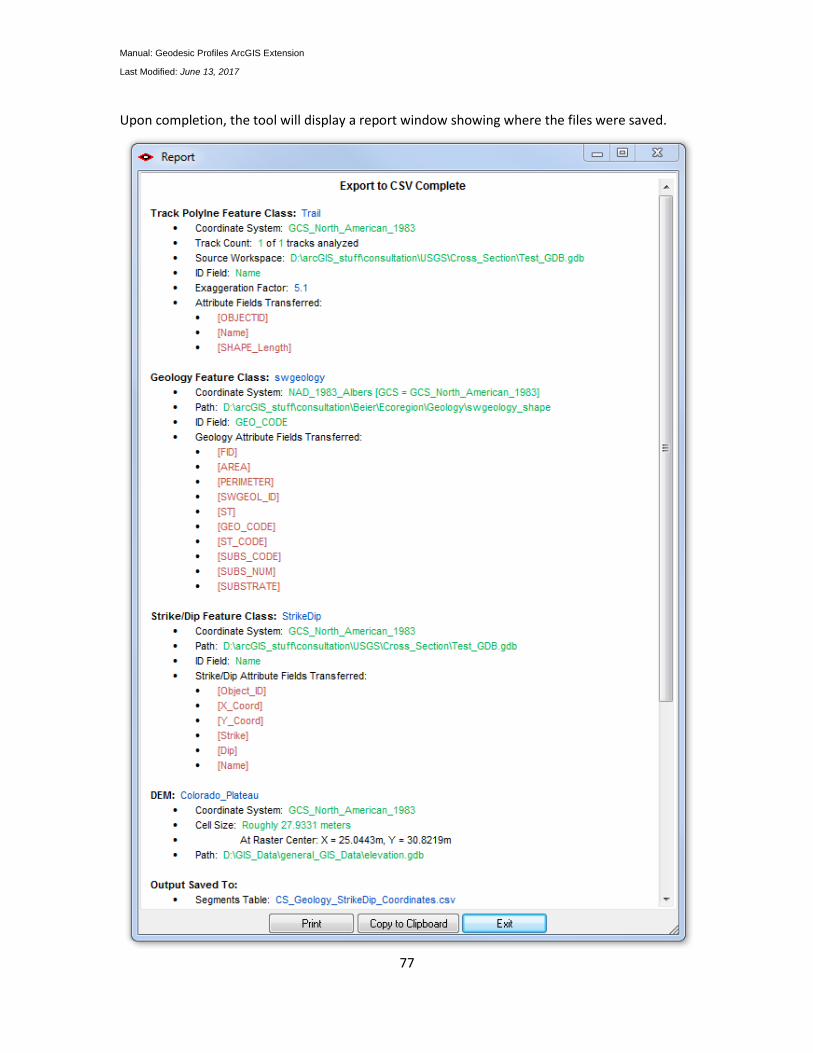
Manual: Geodesic Profiles ArcGIS Extension
Last Modified: June 13, 2017
77
Upon completion, the tool will display a report window showing where the files were saved.
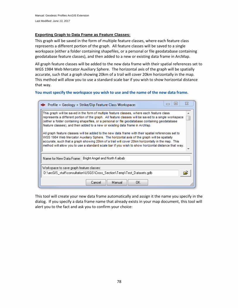
Manual: Geodesic Profiles ArcGIS Extension
Last Modified: June 13, 2017
78
Exporting Graph to Data Frame as Feature Classes:
This graph will be saved in the form of multiple feature classes, where each feature class represents a different portion of the graph. All feature classes will be saved to a single workspace (either a folder containing shapefiles, or a personal or file geodatabase containing geodatabase feature classes), and then added to a new or existing data frame in ArcMap.
All graph feature classes will be added to the new data frame with their spatial references set to WGS 1984 Web Mercator Auxiliary Sphere. The horizontal axis of the graph will be spatially accurate, such that a graph showing 20km of a trail will cover 20km horizontally in the map. This method will allow you to use a standard scale bar if you wish to show horizontal distance that way.
You must specify the workspace you wish to use and the name of the new data frame.
This tool will create your new data frame automatically and assign it the name you specify in the dialog. If you specify a data frame name that already exists in your map document, this tool will alert you to the fact and ask you to confirm your choice:

Manual: Geodesic Profiles ArcGIS Extension
Last Modified: June 13, 2017
79
All datasets will be named automatically, based on the name of your Track/Route layer.
Details: This tool will create11 new feature classes representing different aspects of the graph.
1) Segments Feature Class: Contains a separate record for each vertex-to-vertex segment along a route. When initially added to the map, it will be symbolized by slope in a blue-to-red color ramp. In addition to any attribute fields from the original route feature class you may choose to transfer, this feature class will also include the following calculated attributes:
Start_Latitude: In the geographic coordinate system of your original Polyline Route feature class.
Start_Longitude: In the geographic coordinate system of your original Polyline Route feature class.
End_Latitude: In the geographic coordinate system of your original Polyline Route feature class.
End_Longitude: In the geographic coordinate system of your original Polyline Route feature class.
Geodesic_Length: The segment length, in meters, calculated using Vincenty's algorithms to estimate geodesic distances over the original Polygon Route feature class spheroid (see Vincenty 1975; also p. 124 of this manual).
Surface_Length: The segment surface length, in meters, calculated using the Pythagorean theorem to determine the hypotenuse of the triangle formed by the change in elevation and the geodesic distance.
Slope_Degrees: The absolute value of the segment slope.
Bearing: The compass bearing of the segment.
Start_Elevation: The elevation value at the beginning of the segment based on the selected DEM, calculated using bilinear interpolation (see p. 106). The vertex is projected into the DEM datum and coordinate system prior to analysis if necessary. If the original DEM is not in meters, then the values are converted to meters in this attribute field.
Manual: Geodesic Profiles ArcGIS Extension
Last Modified: June 13, 2017
80
Mid_Elevation: The elevation value at the centerpoint of the segment.
End_Elevation: The elevation value at the end of the segment.
End_Proportion: The proportion of the original route at the segment endpoint. This proportion is based on the surface distance of the line, not the geodesic distance. Values will range from 0 to 1.
Total_Geodesic_Distance: The total geodesic distance, in meters, along the route up to the end of this segment.
Total_Surface_Distance: The total surface distance, in meters, along the route up to the end of this segment.
2) Polyline Feature Class: Contains a separate record for each route showing the profile of the route over the DEM. When initially added to the map, it will be symbolized by ID value based on the ID field you select. If you do not select an ID field, it will be symbolized by the Feature Object ID of the original route. In addition to any attribute fields from the original route feature class you may choose to transfer, this feature class will also include the following calculated attributes:
Sample_Points: The number of DEM values sampled to generate the statistics for this polyline.
Start_Latitude: In the geographic coordinate system of your original Polyline Route feature class.
Start_Longitude: In the geographic coordinate system of your original Polyline Route feature class.
End_Latitude: In the geographic coordinate system of your original Polyline Route feature class.
End_Longitude: In the geographic coordinate system of your original Polyline Route feature class.
Start_Elevation: The elevation value of starting point based on the selected DEM, calculated using bilinear interpolation (see p. 106). The vertex is projected into the DEM datum and coordinate system prior to analysis if necessary. If the original DEM is not in meters, then the values are converted to meters in this table.
End_Elevation: The elevation of the ending point based on the selected DEM.
Min_Elevation: The elevation of the lowest point based on the selected DEM.
Max_Elevation: The elevation of the highest point based on the selected DEM.
Avg_Slope: The average slope over the course of the route, calculated as the weighted mean of the segment slopes, weighted by the segment surface distances.
Slope_StDev: The standard deviation of slope over the course of the route.
Avg_Bearing: The mean direction of the route, equal to the bearing from the starting point to the ending point of the route.

Manual: Geodesic Profiles ArcGIS Extension
Last Modified: June 13, 2017
81
BearingMRL: The Mean Resultant Length of the route, calculated as the ratio of the geodesic length of the complete route divided by the geodesic distance of the straight line between the starting and ending points. The MRL is the basis of several circular measures of dispersion (see Batschelet 1981, Fisher 1995, Mardia and Jupp 2000). MRL values near 1 indicate little direction variation over the line.
Length_Geodesic: The geodesic length of the route.
Length_Surface: The surface length of the route.
Surface Ratio: The ratio of [Surface Length] / [Geodesic Length]. Values near 1 indicate a flat line, while values > 1 indicate increasing elevational variation.
3) Polygon Feature Class: Similar to the Polyline Feature Class, except that it symbolizes the route using a polygon to symbolize the portion of the graph underneath the route profile. Contains a separate record for each route. When initially added to the map, it will be symbolized by ID value based on the ID field you select. If you do not select an ID field, it will be symbolized by the Feature Object ID of the original route. This feature class will contain exactly the same attribute fields and values as the Polyline Feature Class described above.
4) Clipped Polyline Feature Class: Contains a separate record for each intersection between the route and a geology polygon, showing the profile of the route over the DEM. When initially added to the map, it will be symbolized by the color of the Geology polygons. In addition to any attribute fields from the original route and geology feature classes you may choose to transfer, this feature class will also include the following calculated attributes:
Sample_Points: The number of DEM values sampled to generate the statistics for this clipped portion of the route polyline.
Start_Latitude: In the geographic coordinate system of your original Polyline Route feature class.
Start_Longitude: In the geographic coordinate system of your original Polyline Route feature class.
End_Latitude: In the geographic coordinate system of your original Polyline Route feature class.
End_Longitude: In the geographic coordinate system of your original Polyline Route feature class.
Start_Elevation: The elevation value of starting point based on the selected DEM, calculated using Bilinear Interpolation. The vertex is projected into the DEM datum and coordinate system prior to analysis if necessary. If the original DEM is not in meters, then the values are converted to meters in this table.
End_Elevation: The elevation of the ending point based on the selected DEM.
Min_Elevation: The elevation of the lowest point based on the selected DEM.
Max_Elevation: The elevation of the highest point based on the selected DEM.
Avg_Slope: The average slope over the course of the route, calculated as the weighted mean of the segment slopes, weighted by the segment surface distances.

Manual: Geodesic Profiles ArcGIS Extension
Last Modified: June 13, 2017
82
Slope_StDev: The standard deviation of slope over the course of the route.
Avg_Bearing: The mean direction of the route, equal to the bearing from the starting point to the ending point of the route.
BearingMRL: The Mean Resultant Length of the route, calculated as the ratio of the geodesic length of the complete route divided by the geodesic distance of the straight line between the starting and ending points. The MRL is the basis of several circular measures of dispersion (see Batschelet 1981, Fisher 1995, Mardia and Jupp 2000). MRL values near 1 indicate little direction variation over the line.
Length_Geodesic: The geodesic length of the route.
Length_Surface: The surface length of the route.
Surface_Ratio: The ratio of [Surface Length] / [Geodesic Length]. Values near 1 indicate a flat line, while values > 1 indicate increasing elevational variation.
Start_Position_Geodesic: The geodesic distance of the beginning of this clipped section, as located on the original route feature.
End_Position_Geodesic: The geodesic distance of the end of this clipped section, as located on the original route feature.
5) Clipped Polyline Tic Mark Feature Class: Contains a separate record for the intersection points between the route and geology polygons, showing a short vertical line that intersects the profile line. This feature class is intended primarily to add aesthetic qualities to the profile graph. When initially added to the map, it will be symbolized by the color of the Geology polygons. This feature class will only include the following calculated attributes:
Left_GeoID: The geology polygon ID value on the left side of the tick mark.
Right_GeoID: The geology polygon ID value on the right side of the tick mark.
Label_Value: A string value composed of [Left_GeoID] + a vertical line ("|") + [Right_GeoID]. This might be useful for labeling purposes in the graph.
Position_Geodesic: The geodesic distance of this point, as located on the original route feature.
Elevation: The elevation, in meters, at this point.
Latitude: In the geographic coordinate system of your original Polyline Route feature class.
Longitude: In the geographic coordinate system of your original Polyline Route feature class.
6) Clipped Polyline Vertical Line Feature Class: Contains a separate record for the intersection points between the route and geology polygons, showing a vertical line that extends from the bottom of the graph up to the profile line. This feature class is intended primarily to add aesthetic qualities to the profile graph. When initially added to the map, it will be symbolized
Manual: Geodesic Profiles ArcGIS Extension
Last Modified: June 13, 2017
83
by the color of the Geology polygons. This feature class will only include the following calculated attributes:
Left_GeoID: The geology polygon ID value on the left side of the line.
Right_GeoID: The geology polygon ID value on the right side of the line.
Label_Value: A string value composed of [Left_GeoID] + a vertical line ("|") + [Right_GeoID]. This might be useful for labeling purposes in the graph.
Position_Geodesic: The geodesic distance of this point, as located on the original route feature.
Elevation: The elevation, in meters, at this point.
Latitude: In the geographic coordinate system of your original Polyline Route feature class.
Longitude: In the geographic coordinate system of your original Polyline Route feature class.
7) Strike/Dip Route-Plane Vertices: Describes the linear intersection between the Strike/Dip plane (as defined by a single point with Strike and Dip angle attributes) and the original route projected vertically down onto that plane. Each point in the feature class will describe a vertex or sample point along the original route, along with statistics on route and strike/dip plane values at that point. In addition to any attribute fields from the original route and strike/dip feature classes you may choose to transfer, this feature class will also include the following calculated attributes:
Latitude: In the geographic coordinate system of your original Polyline Route feature class.
Longitude: In the geographic coordinate system of your original Polyline Route feature class.
Compass_Bearing: The compass bearing from the previous vertex to this vertex. The first record will have a compass bearing = -999.
Route_Elevation_Meters: The elevation value of this vertex based on the selected DEM, calculated using Bilinear Interpolation. The vertex is projected into the DEM datum and coordinate system prior to analysis if necessary. If the original DEM is not in meters, then the values are converted to meters in this table.
Plane_Elevation_Meters: The elevation value of this location on the Strike/Dip Plane defined by this particular Strike/Dip point.
Elevation_Difference: The elevation value of the Route at this location, minus the elevation on the Strike/Dip Plane at this location.
Cumulative_Geodesic_Distance_Meters: The total geodesic distance along the route up to this vertex, calculated using Vincenty's algorithms to estimate geodesic distances over the original Polygon Route feature class spheroid (see Vincenty 1975; also p. 124 of this manual).
Manual: Geodesic Profiles ArcGIS Extension
Last Modified: June 13, 2017
84
Cumulative_Proportion: The proportion of the original route at this vertex. This proportion is based on the surface distance of the original route, not the geodesic distance of the route or the distance along the strike/dip plane.
Exaggeration_Factor: The exaggeration factor used to adjust the dimensions of the profile graph. This may be useful if you wish to generate a profile graph from these points in some other software package such as R.
Exaggerated_Plane_Elevation: The elevation of the strike/dip plane point after being multiplied by the exaggeration factor. This is the value that is actually being plotted on the graph, and this value may also be useful if you wish to generate a profile graph from these points in some other software package.
8) Strike/Dip Route-Plane Polylines: Describes the linear intersection between the Strike/Dip plane (as defined by a single point with Strike and Dip angle attributes) and the original route projected vertically down onto that plane. Each polyline in the feature class will describe the portion of the strike/dip plane that lies directly beneath the route polyline. If the ground surface extends below the strike/dip plane along any portion of the route, then those portions will be excluded from the dataset. If a single strike/dip plane is broken up this way, then each sub-portion of the final polyline will be saved as a separate feature in the feature class. In addition to any attribute fields from the original route and strike/dip feature classes you may choose to transfer, this feature class will also include the following calculated attributes:
Start_Latitude: In the geographic coordinate system of your original Polyline Route feature class.
Start_Longitude: In the geographic coordinate system of your original Polyline Route feature class.
End_Latitude: In the geographic coordinate system of your original Polyline Route feature class.
End_Longitude: In the geographic coordinate system of your original Polyline Route feature class.
Start_Elevation: The elevation value of the Strike/Dip segment starting point based on the Strike/Dip plane.
End_Elevation: The elevation of the Strike/Dip segment ending point based on the Strike/Dip plane.
Length_Geodesic: The geodesic length of the route.
Start_Position_Geodesic: The geodesic distance of the beginning of this portion of the original route.
End_Position_Geodesic: The geodesic distance of the ending of this portion of the original route.
Start_Proportion: The position of the beginning of this portion of the original route, expressed as a proportion of the entire original route.
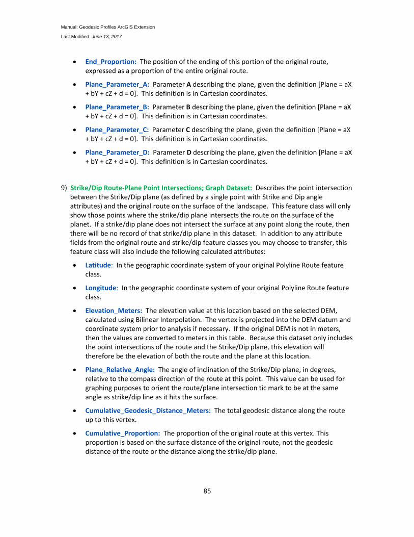
Manual: Geodesic Profiles ArcGIS Extension
Last Modified: June 13, 2017
85
End_Proportion: The position of the ending of this portion of the original route, expressed as a proportion of the entire original route.
Plane_Parameter_A: Parameter A describing the plane, given the definition [Plane = aX + bY + cZ + d = 0]. This definition is in Cartesian coordinates.
Plane_Parameter_B: Parameter B describing the plane, given the definition [Plane = aX + bY + cZ + d = 0]. This definition is in Cartesian coordinates.
Plane_Parameter_C: Parameter C describing the plane, given the definition [Plane = aX + bY + cZ + d = 0]. This definition is in Cartesian coordinates.
Plane_Parameter_D: Parameter D describing the plane, given the definition [Plane = aX + bY + cZ + d = 0]. This definition is in Cartesian coordinates.
9) Strike/Dip Route-Plane Point Intersections; Graph Dataset: Describes the point intersection between the Strike/Dip plane (as defined by a single point with Strike and Dip angle attributes) and the original route on the surface of the landscape. This feature class will only show those points where the strike/dip plane intersects the route on the surface of the planet. If a strike/dip plane does not intersect the surface at any point along the route, then there will be no record of that strike/dip plane in this dataset. In addition to any attribute fields from the original route and strike/dip feature classes you may choose to transfer, this feature class will also include the following calculated attributes:
Latitude: In the geographic coordinate system of your original Polyline Route feature class.
Longitude: In the geographic coordinate system of your original Polyline Route feature class.
Elevation_Meters: The elevation value at this location based on the selected DEM, calculated using Bilinear Interpolation. The vertex is projected into the DEM datum and coordinate system prior to analysis if necessary. If the original DEM is not in meters, then the values are converted to meters in this table. Because this dataset only includes the point intersections of the route and the Strike/Dip plane, this elevation will therefore be the elevation of both the route and the plane at this location.
Plane_Relative_Angle: The angle of inclination of the Strike/Dip plane, in degrees, relative to the compass direction of the route at this point. This value can be used for graphing purposes to orient the route/plane intersection tic mark to be at the same angle as strike/dip line as it hits the surface.
Cumulative_Geodesic_Distance_Meters: The total geodesic distance along the route up to this vertex.
Cumulative_Proportion: The proportion of the original route at this vertex. This proportion is based on the surface distance of the original route, not the geodesic distance of the route or the distance along the strike/dip plane.
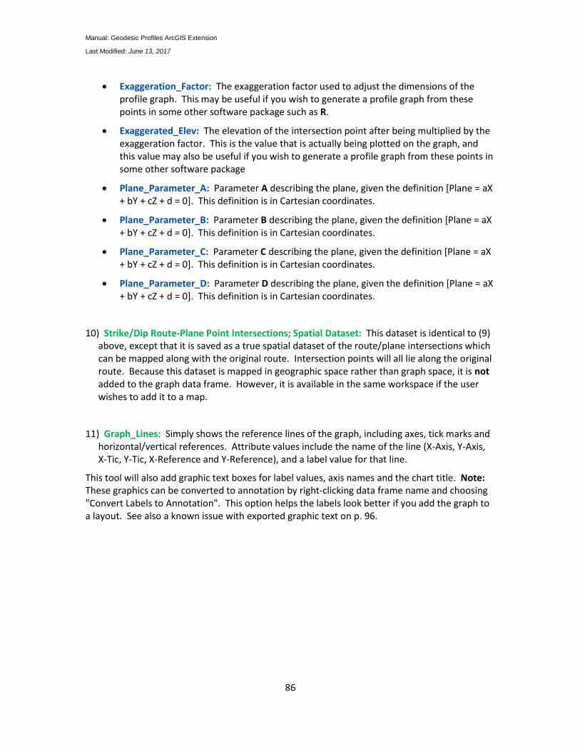
Manual: Geodesic Profiles ArcGIS Extension
Last Modified: June 13, 2017
86
Exaggeration_Factor: The exaggeration factor used to adjust the dimensions of the profile graph. This may be useful if you wish to generate a profile graph from these points in some other software package such as R.
Exaggerated_Elev: The elevation of the intersection point after being multiplied by the exaggeration factor. This is the value that is actually being plotted on the graph, and this value may also be useful if you wish to generate a profile graph from these points in some other software package
Plane_Parameter_A: Parameter A describing the plane, given the definition [Plane = aX + bY + cZ + d = 0]. This definition is in Cartesian coordinates.
Plane_Parameter_B: Parameter B describing the plane, given the definition [Plane = aX + bY + cZ + d = 0]. This definition is in Cartesian coordinates.
Plane_Parameter_C: Parameter C describing the plane, given the definition [Plane = aX + bY + cZ + d = 0]. This definition is in Cartesian coordinates.
Plane_Parameter_D: Parameter D describing the plane, given the definition [Plane = aX + bY + cZ + d = 0]. This definition is in Cartesian coordinates.
10) Strike/Dip Route-Plane Point Intersections; Spatial Dataset: This dataset is identical to (9) above, except that it is saved as a true spatial dataset of the route/plane intersections which can be mapped along with the original route. Intersection points will all lie along the original route. Because this dataset is mapped in geographic space rather than graph space, it is not added to the graph data frame. However, it is available in the same workspace if the user wishes to add it to a map.
11) Graph_Lines: Simply shows the reference lines of the graph, including axes, tick marks and horizontal/vertical references. Attribute values include the name of the line (X-Axis, Y-Axis, X-Tic, Y-Tic, X-Reference and Y-Reference), and a label value for that line.
This tool will also add graphic text boxes for label values, axis names and the chart title. Note: These graphics can be converted to annotation by right-clicking data frame name and choosing "Convert Labels to Annotation". This option helps the labels look better if you add the graph to a layout. See also a known issue with exported graphic text on p. 96.
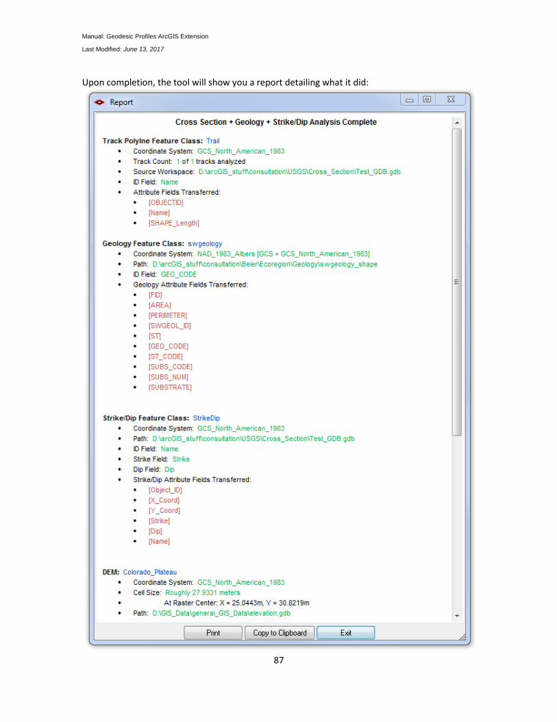
Manual: Geodesic Profiles ArcGIS Extension
Last Modified: June 13, 2017
87
Upon completion, the tool will show you a report detailing what it did:
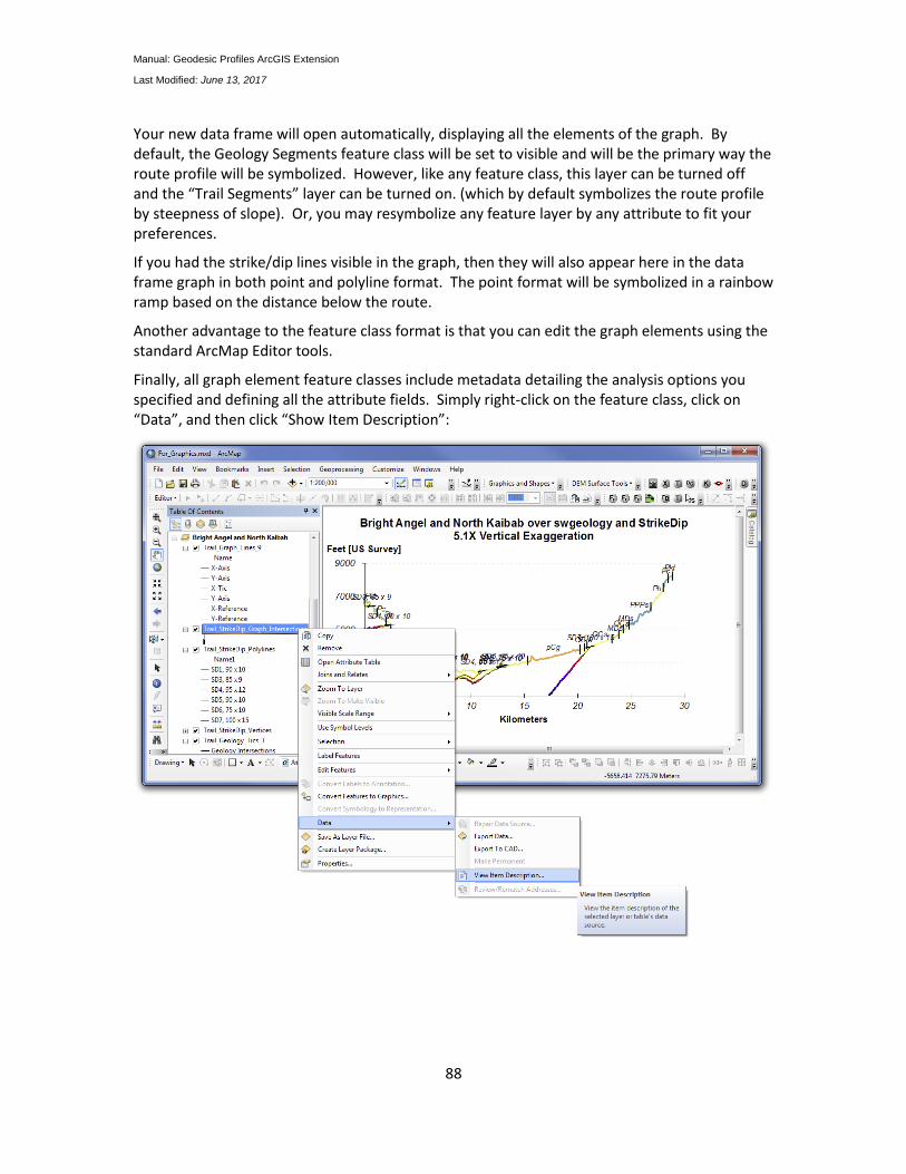
Manual: Geodesic Profiles ArcGIS Extension
Last Modified: June 13, 2017
88
Your new data frame will open automatically, displaying all the elements of the graph. By default, the Geology Segments feature class will be set to visible and will be the primary way the route profile will be symbolized. However, like any feature class, this layer can be turned off and the “Trail Segments” layer can be turned on. (which by default symbolizes the route profile by steepness of slope). Or, you may resymbolize any feature layer by any attribute to fit your preferences.
If you had the strike/dip lines visible in the graph, then they will also appear here in the data frame graph in both point and polyline format. The point format will be symbolized in a rainbow ramp based on the distance below the route.
Another advantage to the feature class format is that you can edit the graph elements using the standard ArcMap Editor tools.
Finally, all graph element feature classes include metadata detailing the analysis options you specified and defining all the attribute fields. Simply right-click on the feature class, click on “Data”, and then click “Show Item Description”:
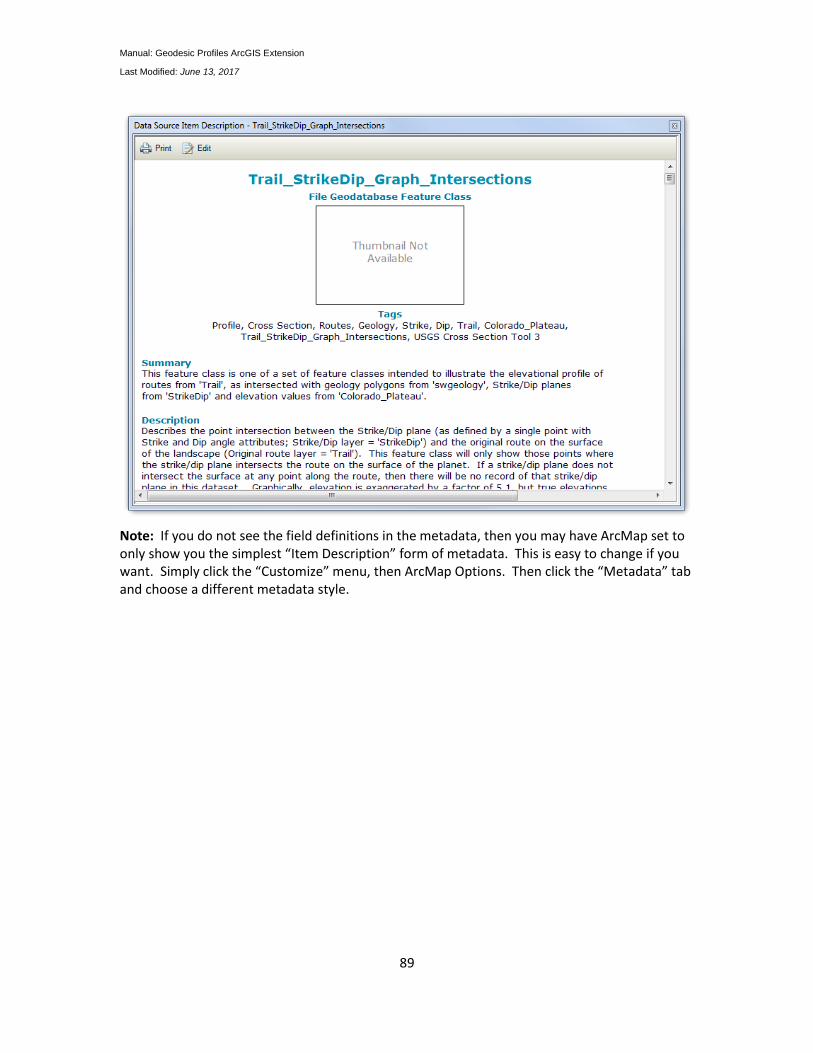
Manual: Geodesic Profiles ArcGIS Extension
Last Modified: June 13, 2017
89
Note: If you do not see the field definitions in the metadata, then you may have ArcMap set to only show you the simplest “Item Description” form of metadata. This is easy to change if you want. Simply click the “Customize” menu, then ArcMap Options. Then click the “Metadata” tab and choose a different metadata style.
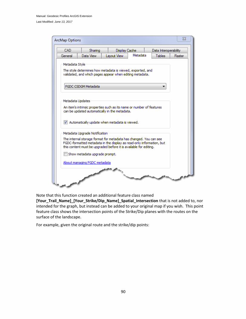
Manual: Geodesic Profiles ArcGIS Extension
Last Modified: June 13, 2017
90
Note that this function created an additional feature class named [Your_Trail_Name]_[Your_Strike/Dip_Name]_Spatial_Intersection that is not added to, nor intended for the graph, but instead can be added to your original map if you wish. This point feature class shows the intersection points of the Strike/Dip planes with the routes on the surface of the landscape.
For example, given the original route and the strike/dip points:
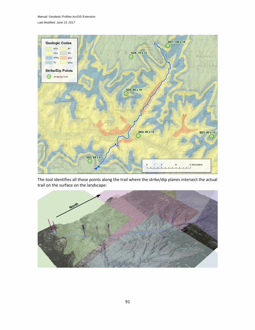
Manual: Geodesic Profiles ArcGIS Extension
Last Modified: June 13, 2017
91
The tool identifies all those points along the trail where the strike/dip planes intersect the actual trail on the surface on the landscape:
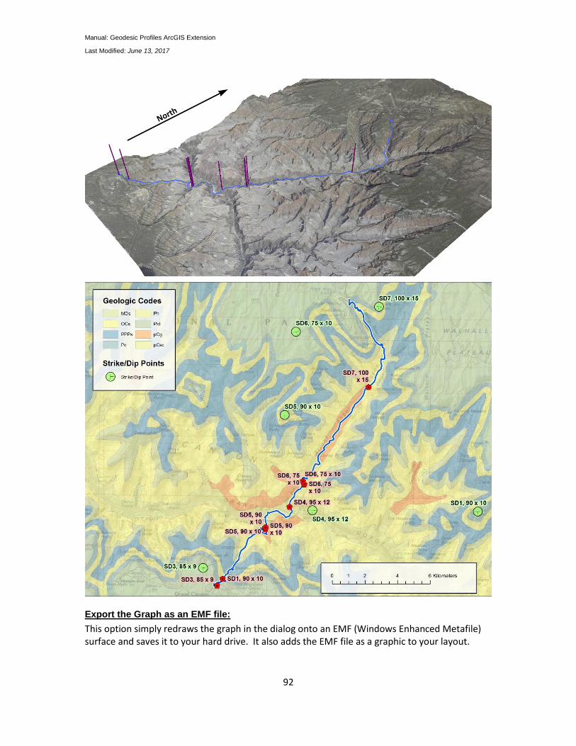
Manual: Geodesic Profiles ArcGIS Extension
Last Modified: June 13, 2017
92
Export the Graph as an EMF file:
This option simply redraws the graph in the dialog onto an EMF (Windows Enhanced Metafile) surface and saves it to your hard drive. It also adds the EMF file as a graphic to your layout.
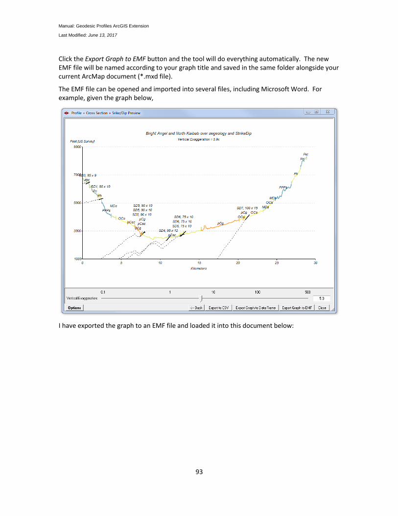
Manual: Geodesic Profiles ArcGIS Extension
Last Modified: June 13, 2017
93
Click the Export Graph to EMF button and the tool will do everything automatically. The new EMF file will be named according to your graph title and saved in the same folder alongside your current ArcMap document (*.mxd file).
The EMF file can be opened and imported into several files, including Microsoft Word. For example, given the graph below,
I have exported the graph to an EMF file and loaded it into this document below:
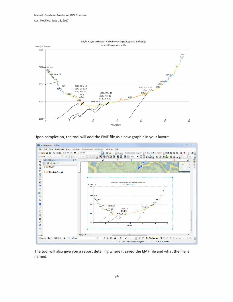
Manual: Geodesic Profiles ArcGIS Extension
Last Modified: June 13, 2017
94
Upon completion, the tool will add the EMF file as a new graphic in your layout.
The tool will also give you a report detailing where it saved the EMF file and what the file is named:
1000
0
9000
3000
5000
7000
Feet [US Survey]
305 10 15 20 25
Kilometers
Vertical Exaggeration = 5.9x
Pkt
Pc
Ph
PPPs
MDs
OCspCsc
pCg
pCsc
pCg
pCsc
pCg
OCs
pCg OCs
MDs
OCs
MDs
PPPs
Ph
Pc
Pkt
SD1, 90 x 10
SD3, 85 x 9
SD4, 95 x 12
SD5, 90 x 10
SD5, 90 x 10
SD5, 90 x 10
SD6, 75 x 10
SD6, 75 x 10
SD6, 75 x 10
SD7, 100 x 15
Bright Angel and North Kaibab over swgeology and StrikeDip
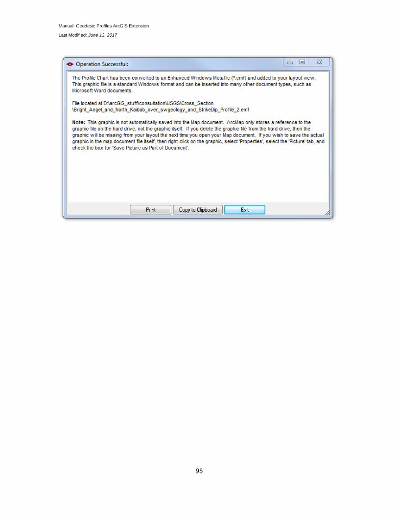
Manual: Geodesic Profiles ArcGIS Extension
Last Modified: June 13, 2017
95
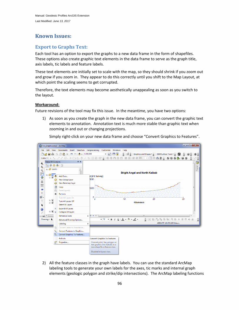
Manual: Geodesic Profiles ArcGIS Extension
Last Modified: June 13, 2017
96
Known Issues:
Export to Graphs Text:
Each tool has an option to export the graphs to a new data frame in the form of shapefiles. These options also create graphic text elements in the data frame to serve as the graph title, axis labels, tic labels and feature labels.
These text elements are initially set to scale with the map, so they should shrink if you zoom out and grow if you zoom in. They appear to do this correctly until you shift to the Map Layout, at which point the scaling seems to get corrupted.
Therefore, the text elements may become aesthetically unappealing as soon as you switch to the layout.
Workaround:
Future revisions of the tool may fix this issue. In the meantime, you have two options:
1) As soon as you create the graph in the new data frame, you can convert the graphic text elements to annotation. Annotation text is much more stable than graphic text when zooming in and out or changing projections.
Simply right-click on your new data frame and choose “Convert Graphics to Features”.
2) All the feature classes in the graph have labels. You can use the standard ArcMap labeling tools to generate your own labels for the axes, tic marks and internal graph elements (geologic polygon and strike/dip intersections). The ArcMap labeling functions
Manual: Geodesic Profiles ArcGIS Extension
Last Modified: June 13, 2017
97
(especially using the Maplex label engine) may work better at placing graph labels than this extension anyway.
Incorrect Elevations if route does not lie completely within DEM:
Currently this tool interprets null DEM values to be a very large negative number. Therefore if the route goes off the edge of a DEM, goes through a hole in the DEM or otherwise goes over null cells, then the elevation at those points may be interpreted to be something odd and unreasonable like -3280800 or -99999.
Workaround:
Currently the only workaround is to use a new DEM raster that completely encompasses the route(s).
Manual: Geodesic Profiles ArcGIS Extension
Last Modified: June 13, 2017
98
Planetocentric vs. Planetographic Coordinate Systems
This tool is designed to assist in the analysis of the surface of non-terrestrial sites, such as other planets, the Earth’s moon, or the moons of other planets. The shapes of these large objects are often modeled with an oblate ellipsoid (similar to a sphere, but squashed vertically around the axis of rotation). All well and good, but we run into an issue with how latitude is defined on Earth vs. other planetary objects.
Latitudes on Earth are generally reported in geodetic coordinates, while latitudes on non-terrestrial objects are generally reported in geocentric coordinates (not to be confused with the “geocentric model of the universe”, where everything rotates around the Earth. In fact, the concept would be more accurately referred to as planetocentric coordinates, which are explained on p. 135).
This tool would be marginally more accurate if it converted all planetocentric latitude/longitude values to planetographic before analysis, since the distance and direction functions assume planetographic coordinates. However, the author of this tool has not figured out a way to determine automatically whether a given coordinate system is based on a planetographic vs. a planetocentric datum. Therefore, the only way to guarantee that these conversions are made is to require the user to specify whether each input dataset comes from a planetographic vs. planetocentric coordinate system, which has the potential to cause much more confusion that it would solve.
With regards to the actual profile charts, any planetographic vs. planetocentric error is likely to be so small as to be unnoticeable. Also, if the underlying datum is a sphere rather than an oblate ellipsoid, then there will be no error because planetographic and planetocentric coordinates are the same in this case.
If users desire that this tool should correctly transform between planetographic and planetocentric coordinates, then please contact the author at [email protected] and let’s discuss. There are internal functions in the code that can make this conversion, so the only issue is how to specify that the conversion is needed. Maybe we can come up with a creative way to let the tool know.
Manual: Geodesic Profiles ArcGIS Extension
Last Modified: June 13, 2017
99
Citations Auroux, D. 2007. Session 16: Intersection of a Line and a Plane.
<http://ocw.mit.edu/courses/mathematics/18-02sc-multivariable-calculus-fall-2010/1.-vectors-and-matrices/part-c-parametric-equations-for-curves/session-16-intersection-of-a-line-and-a-plane/>. Accessed 22 Jun 2016.
Batschelet, E. 1981. Circular statistics in biology. Academic Press, London; New York. Chovitz, B. 2002. In Memoriam: Thaddeus Vincenty. IAG Newsletter.
<http://www.gfy.ku.dk/~iag/newslett/news7606.htm>. Accessed 4 Feb 2016. Dawkins, P. 2016a. Equations of Planes. Paul’s Online Math Notes.
<http://tutorial.math.lamar.edu/Classes/CalcIII/EqnsOfPlanes.aspx>. Accessed 21 Jun 2016.
Dawkins, P. 2016b. Vectors - The Basics. Calculus II - Notes. <http://tutorial.math.lamar.edu/Classes/CalcII/Vectors_Basics.aspx>. Accessed 22 Jun 2016.
Fisher, N. I. 1995. Statistical analysis of circular data. Cambridge University Press, Cambridge [England]; New York.
Iliffe, J. 2000. Datums and Map Projections for remote sensing, GIS, and surveying. CRC Press. Jammalamadaka, S. R., and A. SenGupta. 2001. Topics in circular statistics. World Scientific, River
Edge, N.J. <http://site.ebrary.com/id/10255767>. Accessed 27 Jun 2012. Jenness, J. 2015. Polar Plots for ArcGIS. English, Jenness Enterprises.
<http://www.jennessent.com/arcgis/polar_plots.htm>. Accessed 22 Jun 2016. Jorge. 2009. Recording planes with strike or dip? The problem of the right-hand rules. Structural
Geology. Blog. <http://www.structuralgeology.org/2009/11/strike-dip-right-hand-rule.html>. Accessed 21 Jun 2016.
Mardia, K. V., and P. E. Jupp. 2000. Directional statistics. Wiley, New York. Meyer, C. D. 2000. Matrix analysis and applied linear algebra. Volume 2. Siam. Mitra, D. 2012. Determine where a vector will intersect a plane. StackExchange Mathematics.
<http://math.stackexchange.com/questions/100439/determine-where-a-vector-will-intersect-a-plane>. Accessed 22 Jun 2016.
Rocscience. 2016. What is the right-hand rule in Dips? <https://support.rocscience.com/hc/en-us/articles/206733447-What-is-the-right-hand-rule-in-Dips->. Accessed 21 Jun 2016.
Seyfarth, E.-A., and F. G. Barth. 1972. Compound slit sense organs on the spider leg: Mechanoreceptors involved in kinesthetic orientation. Journal of Comparative Physiology A: Neuroethology, Sensory, Neural, and Behavioral Physiology 78:176–191.
Snyder, J. P. 1987. Map projections–A working manual. Volume 1395. US Government Printing Office.
Varian. 2004. DreamColor: A Color Reference Guide. Varian’s DREAMVIEW. <http://www.varian.net/dreamview/dreamcolor/earth.html>. Accessed 21 Jun 2016.
Veness, C. 2015a. Calculate distance, bearing and more between two latitude/longitude points. Movable Type Scripts. <http://www.movable-type.co.uk/scripts/latlong.html>. Accessed 4 Feb 2016.
Veness, C. 2015b. Vincenty formula for distance between two latitude/longitude points. Movable Type Scripts. <http://www.movable-type.co.uk/scripts/latlong.html>. Accessed 4 Feb 2016.
Vincenty, T. 1975. Direct and inverse solutions of geodesics on the ellipsoid with application of nested equations. Survey review 23:88–93.

Manual: Geodesic Profiles ArcGIS Extension
Last Modified: June 13, 2017
100
Zar, Jerrold H. 1999. Biostatistical Analysis. 4th edition. Pearson Education.
Manual: Geodesic Profiles ArcGIS Extension
Last Modified: June 13, 2017
101
Revisions Version 1.0.808 (June 14, 2016):
Initial Release
Version 1.0.858 (June 23, 2016):
Fixed error in which the output graph composed of feature classes would have the options for specifying vertical and horizontal guide lines reversed. For example, if the user wanted lines drawn horizontally across the graph at each Y-axis tic mark, but did not want vertical lines drawn at each X-axis tic mark, then the “Export Graph to Data Frame” would switch these and only draw vertical lines.
Updates to Manual.
Fixed an error in which the graphing functions would crash if there was no change in elevation at all over the course of the line.
Cosmetic changes to various dialogs.
Modified “Export to Data Frame” functions to force ArcMap to switch to data view before adding text elements.
Fixed a scaling issue in the preview graph windows that showed an incorrect exaggeration under certain circumstances.
Fixed a bug that would crash the Preview Options window if maximum values were set < minimum values.
Fixed error in Strike/Dip output feature classes in which the Strike/Dip ID value was not properly added if the user did not specify an ID values, which in turned crashed the symbolization code.
Fixed error in Strike/Dip analysis that would crash the tool if no route vertexes had elevations (i.e. if the route polyline completely missed the DEM raster).
Manual: Geodesic Profiles ArcGIS Extension
Last Modified: June 13, 2017
102
Appendices
Appendix A: Concerning Projections and Datums
All tools analyze multiple datasets, and therefore must accommodate the possibility that those datasets may be mapped in different projections and/or datums. The tool takes a few strategies to maximize accuracy given different coordinate systems.
1) All measures of distance and direction along the route are calculated using spheroidal geometry based on Vincenty’s equations for calculations on the spheroid (Vincenty 1975) with minor algebraic modifications by Veness (Veness 2015a). Therefore all vector data are projected into geographic (Latitude/Longitude) coordinates before analysis.
2) The exception to this rule regards the extraction of elevation values from the DEM. Projecting rasters always introduces error, so this tool will avoid that issue by always projecting the elevation sampling locations into the DEM spatial reference rather than vice versa.
3) Details regarding specific tools:
a) The Elevation Profile of Polyline tool does the following:
i) Sample points are extracted from the Track/Route features at every vertex and at a regular interval, depending on user preferences.
ii) These sample points are projected into the DEM coordinate system.
iii) DEM values are interpolated using bilinear interpolation (see p. 106), and the elevation values are saved with the original unprojected vertex.
b) The Cross Sections tool does the following:
i) Track/Route features are projected into the Geology polygon feature class coordinate system, and used to select all intersecting geologic features.
ii) Track/Route features are intersected with geology polygons to find intersection points along the track. These intersection points are saved as proportion values along the route (i.e. the projected track may intersect a polygon at two points, and these points lie at 50% and 75% along the length of the route). Rather than project the intersection points back into the original track/route coordinate system, the tool just generates new sample points at 50% and 75% along the original feature.
iii) These polygon intersection points, plus all track/route vertices and points along a regular interval, are then projected into the DEM coordinate system to get the elevation values.
c) The Cross Sections with Strike/Dip Lines tool does the following:
i) Track/Route features are projected into the Geology polygon feature class coordinate system as described above.
ii) Strike/Dip points are projected into the Track/Route feature class coordinate system before any analysis is done.
Manual: Geodesic Profiles ArcGIS Extension
Last Modified: June 13, 2017
103
iii) All intersection points derived from strike/dip planes, geology polygon intersections, track/route vertices and regular intervals, are projected into the DEM coordinate system before interpolating elevation values.
4) All necessary projections between coordinate systems in the same datum are handled internally by the tool and do not require inputs from the user. However, if the datasets are in different datums, then the tool might need to get additional information from the user.
There are often multiple ways to convert between datums and ArcMap does not automatically know which geotransformation method is best. However, ArcMap will often alert the user if datasets from different datums are loaded into the same map and give the user the opportunity to specify the correct geotransformation. If the datasets are mapped in different datums, and if the user has specified a geotransformation in the Layer Properties, then this tool will use that geotransformation when projecting datasets.
On the other hand, if the datasets are in different datums and ArcMap can’t find an appropriate geotransformation in the Layer Properties, then the tool will ask you to specify the correct transformation before proceeding.
This tool will look through the current database of transformations and identify which ones are designed to transform between the dataset datums. If the tool can find information on known accuracy of those transformations, and what region they are designed for, then this tool will sort them based on these two factors.
If the tool is able to find appropriate transformations, then it will show you the sorted list in the dialog below and ask you to select the one you wish to use.
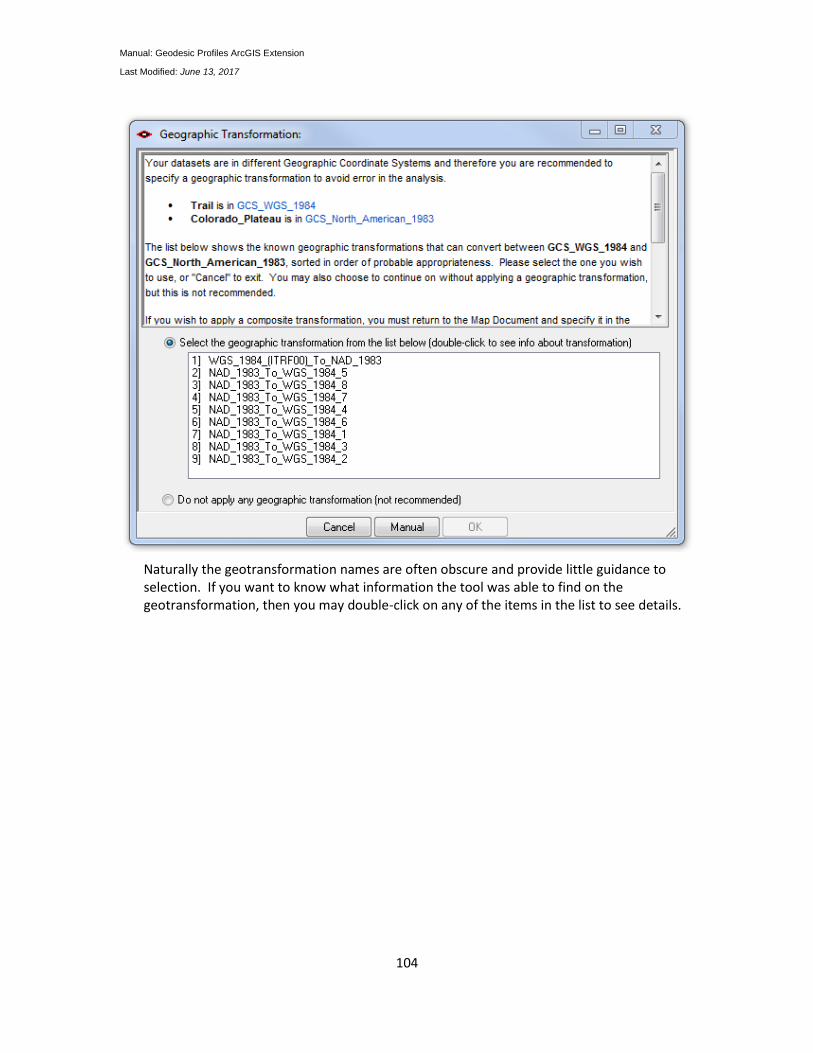
Manual: Geodesic Profiles ArcGIS Extension
Last Modified: June 13, 2017
104
Naturally the geotransformation names are often obscure and provide little guidance to selection. If you want to know what information the tool was able to find on the geotransformation, then you may double-click on any of the items in the list to see details.
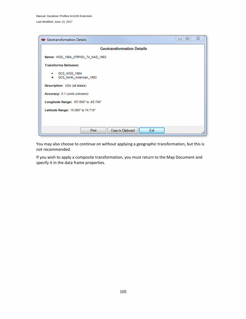
Manual: Geodesic Profiles ArcGIS Extension
Last Modified: June 13, 2017
105
You may also choose to continue on without applying a geographic transformation, but this is not recommended.
If you wish to apply a composite transformation, you must return to the Map Document and specify it in the data frame properties.
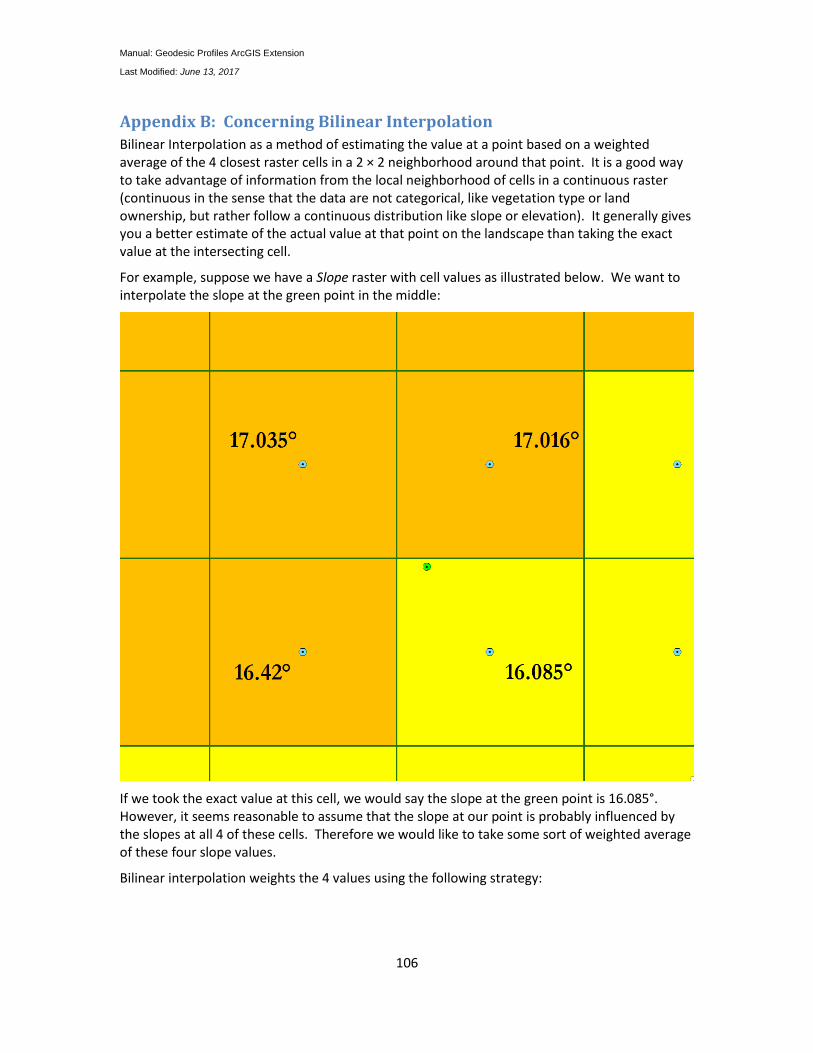
Manual: Geodesic Profiles ArcGIS Extension
Last Modified: June 13, 2017
106
Appendix B: Concerning Bilinear Interpolation
Bilinear Interpolation as a method of estimating the value at a point based on a weighted average of the 4 closest raster cells in a 2 × 2 neighborhood around that point. It is a good way to take advantage of information from the local neighborhood of cells in a continuous raster (continuous in the sense that the data are not categorical, like vegetation type or land ownership, but rather follow a continuous distribution like slope or elevation). It generally gives you a better estimate of the actual value at that point on the landscape than taking the exact value at the intersecting cell.
For example, suppose we have a Slope raster with cell values as illustrated below. We want to interpolate the slope at the green point in the middle:
If we took the exact value at this cell, we would say the slope at the green point is 16.085°. However, it seems reasonable to assume that the slope at our point is probably influenced by the slopes at all 4 of these cells. Therefore we would like to take some sort of weighted average of these four slope values.
Bilinear interpolation weights the 4 values using the following strategy:
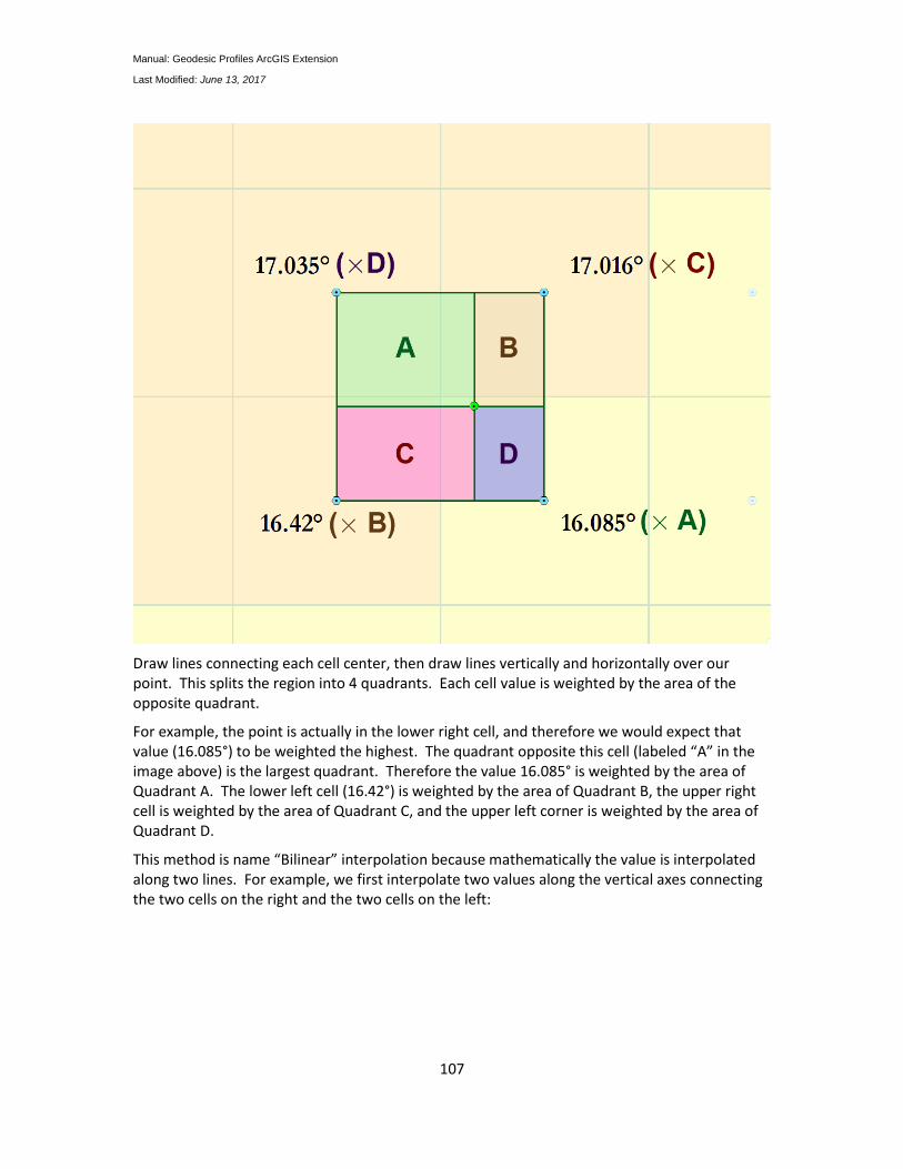
Manual: Geodesic Profiles ArcGIS Extension
Last Modified: June 13, 2017
107
Draw lines connecting each cell center, then draw lines vertically and horizontally over our point. This splits the region into 4 quadrants. Each cell value is weighted by the area of the opposite quadrant.
For example, the point is actually in the lower right cell, and therefore we would expect that value (16.085°) to be weighted the highest. The quadrant opposite this cell (labeled “A” in the image above) is the largest quadrant. Therefore the value 16.085° is weighted by the area of Quadrant A. The lower left cell (16.42°) is weighted by the area of Quadrant B, the upper right cell is weighted by the area of Quadrant C, and the upper left corner is weighted by the area of Quadrant D.
This method is name “Bilinear” interpolation because mathematically the value is interpolated along two lines. For example, we first interpolate two values along the vertical axes connecting the two cells on the right and the two cells on the left:
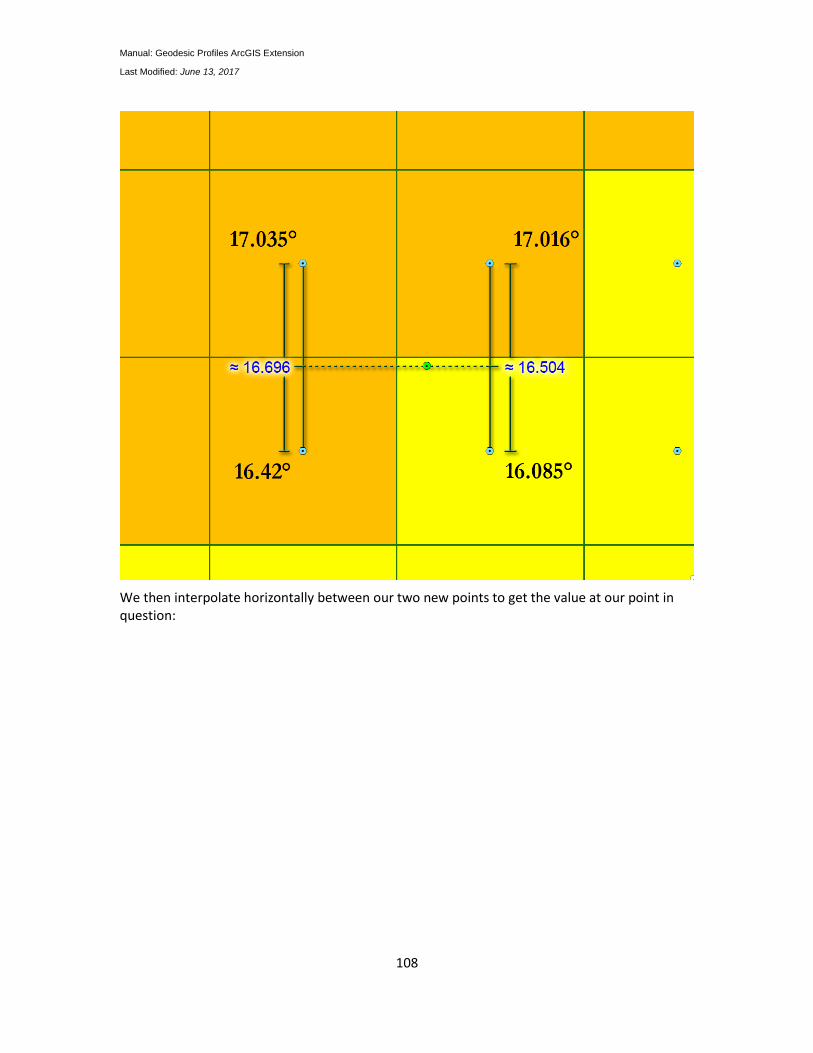
Manual: Geodesic Profiles ArcGIS Extension
Last Modified: June 13, 2017
108
We then interpolate horizontally between our two new points to get the value at our point in question:
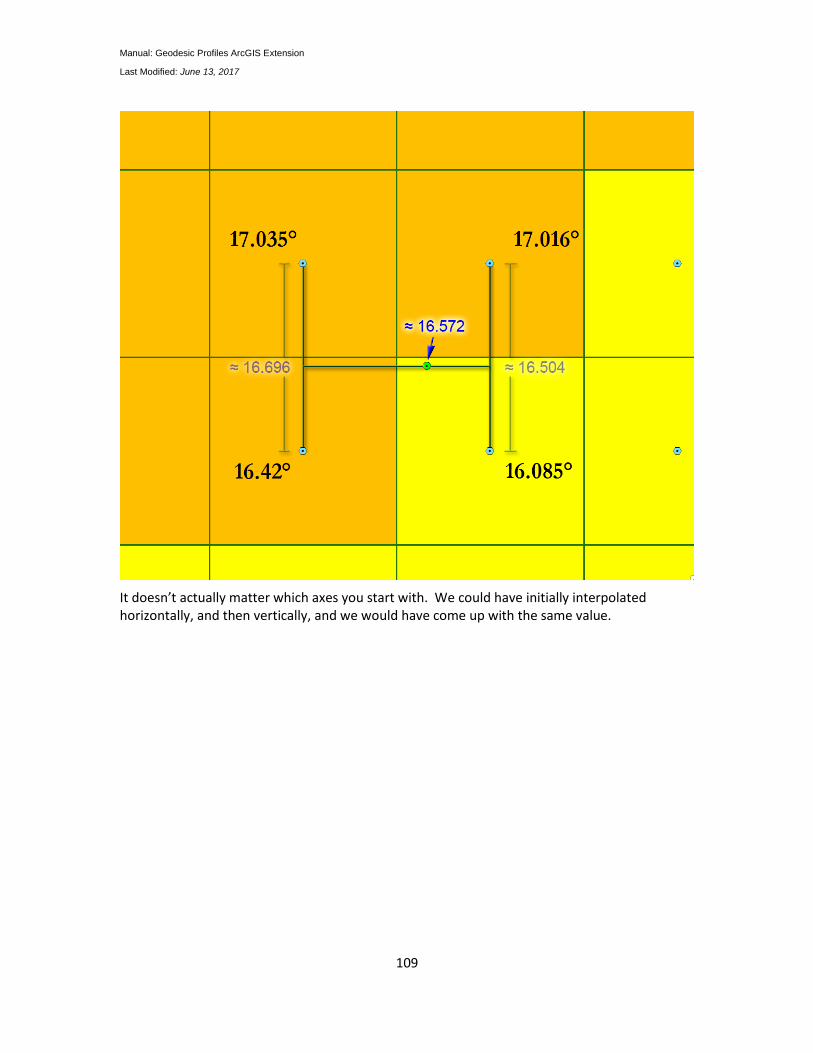
Manual: Geodesic Profiles ArcGIS Extension
Last Modified: June 13, 2017
109
It doesn’t actually matter which axes you start with. We could have initially interpolated horizontally, and then vertically, and we would have come up with the same value.
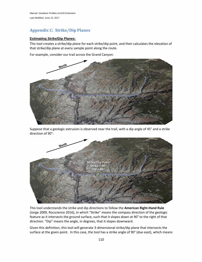
Manual: Geodesic Profiles ArcGIS Extension
Last Modified: June 13, 2017
110
Appendix C: Strike/Dip Planes
Estimating Strike/Dip Planes:
This tool creates a strike/dip plane for each strike/dip point, and then calculates the elevation of that strike/dip plane at every sample point along the route.
For example, consider our trail across the Grand Canyon:
Suppose that a geologic extrusion is observed near the trail, with a dip angle of 45° and a strike direction of 90°:
This tool understands the strike and dip directions to follow the American Right-Hand Rule (Jorge 2009, Rocscience 2016), in which “Strike” means the compass direction of the geologic feature as it intersects the ground surface, such that it slopes down at 90° to the right of that direction. “Dip” means the angle, in degrees, that it slopes downward.
Given this definition, this tool will generate 3-dimensional strike/dip plane that intersects the surface at the given point. In this case, the tool has a strike angle of 90° (due east), which means
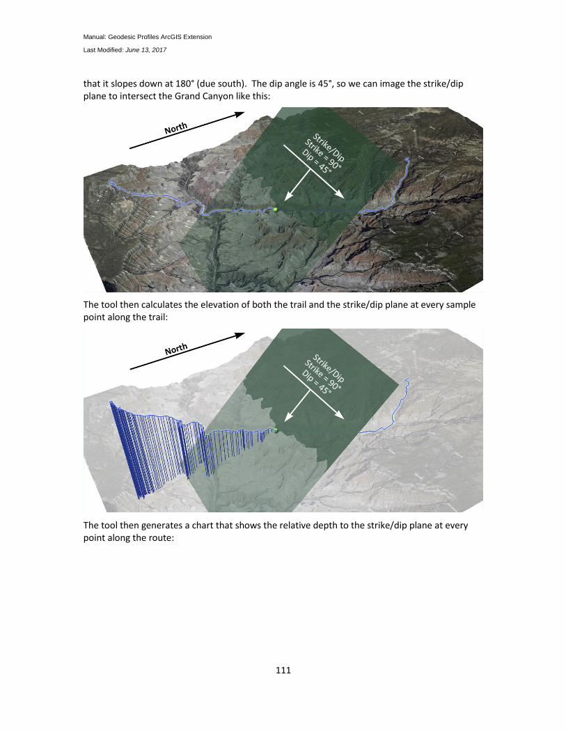
Manual: Geodesic Profiles ArcGIS Extension
Last Modified: June 13, 2017
111
that it slopes down at 180° (due south). The dip angle is 45°, so we can image the strike/dip plane to intersect the Grand Canyon like this:
The tool then calculates the elevation of both the trail and the strike/dip plane at every sample point along the trail:
The tool then generates a chart that shows the relative depth to the strike/dip plane at every point along the route:
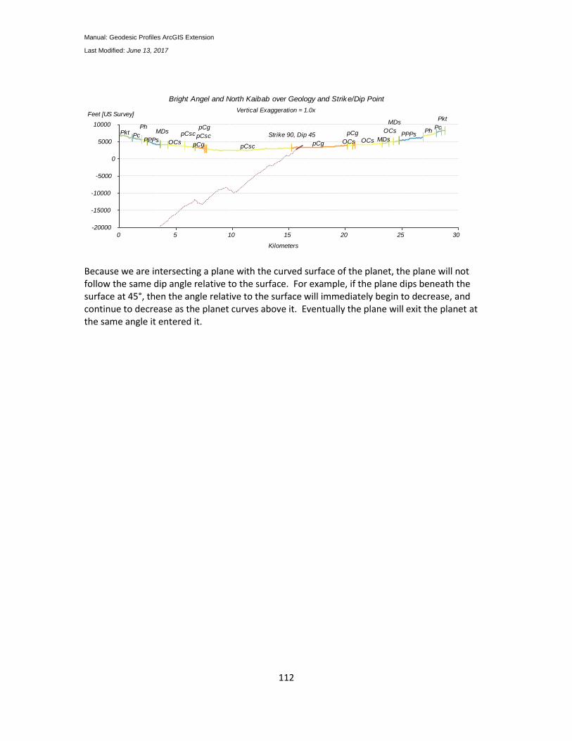
Manual: Geodesic Profiles ArcGIS Extension
Last Modified: June 13, 2017
112
Because we are intersecting a plane with the curved surface of the planet, the plane will not follow the same dip angle relative to the surface. For example, if the plane dips beneath the surface at 45°, then the angle relative to the surface will immediately begin to decrease, and continue to decrease as the planet curves above it. Eventually the plane will exit the planet at the same angle it entered it.
-20000
0
10000
-15000
-10000
-5000
0
5000
Feet [US Survey]
305 10 15 20 25
Kilometers
Vertical Exaggeration = 1.0x
Pkt Pc
Ph
PPPs
MDs
OCs
pCsc
pCg
pCsc
pCg
pCsc pCg OCs
pCg
OCs MDs
OCs
MDs
PPPsPh
Pc
Pkt
Strike 90, Dip 45
Bright Angel and North Kaibab over Geology and Strike/Dip Point
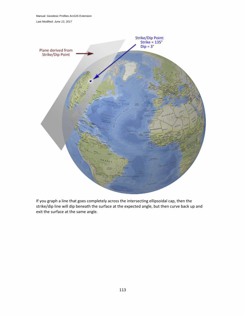
Manual: Geodesic Profiles ArcGIS Extension
Last Modified: June 13, 2017
113
If you graph a line that goes completely across the intersecting ellipsoidal cap, then the strike/dip line will dip beneath the surface at the expected angle, but then curve back up and exit the surface at the same angle.
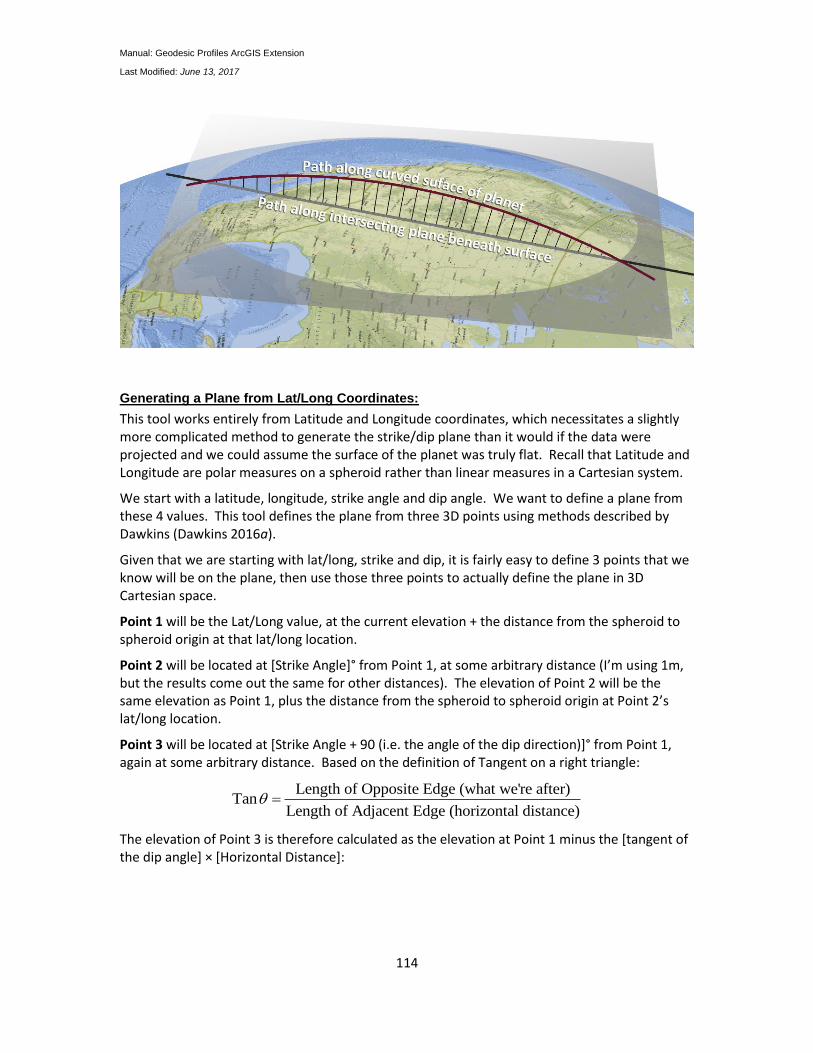
Manual: Geodesic Profiles ArcGIS Extension
Last Modified: June 13, 2017
114
Generating a Plane from Lat/Long Coordinates:
This tool works entirely from Latitude and Longitude coordinates, which necessitates a slightly more complicated method to generate the strike/dip plane than it would if the data were projected and we could assume the surface of the planet was truly flat. Recall that Latitude and Longitude are polar measures on a spheroid rather than linear measures in a Cartesian system.
We start with a latitude, longitude, strike angle and dip angle. We want to define a plane from these 4 values. This tool defines the plane from three 3D points using methods described by Dawkins (Dawkins 2016a).
Given that we are starting with lat/long, strike and dip, it is fairly easy to define 3 points that we know will be on the plane, then use those three points to actually define the plane in 3D Cartesian space.
Point 1 will be the Lat/Long value, at the current elevation + the distance from the spheroid to spheroid origin at that lat/long location.
Point 2 will be located at [Strike Angle]° from Point 1, at some arbitrary distance (I’m using 1m, but the results come out the same for other distances). The elevation of Point 2 will be the same elevation as Point 1, plus the distance from the spheroid to spheroid origin at Point 2’s lat/long location.
Point 3 will be located at [Strike Angle + 90 (i.e. the angle of the dip direction)]° from Point 1, again at some arbitrary distance. Based on the definition of Tangent on a right triangle:
Length of Opposite Edge (what we're after)Tan
Length of Adjacent Edge (horizontal distance)
The elevation of Point 3 is therefore calculated as the elevation at Point 1 minus the [tangent of the dip angle] × [Horizontal Distance]:
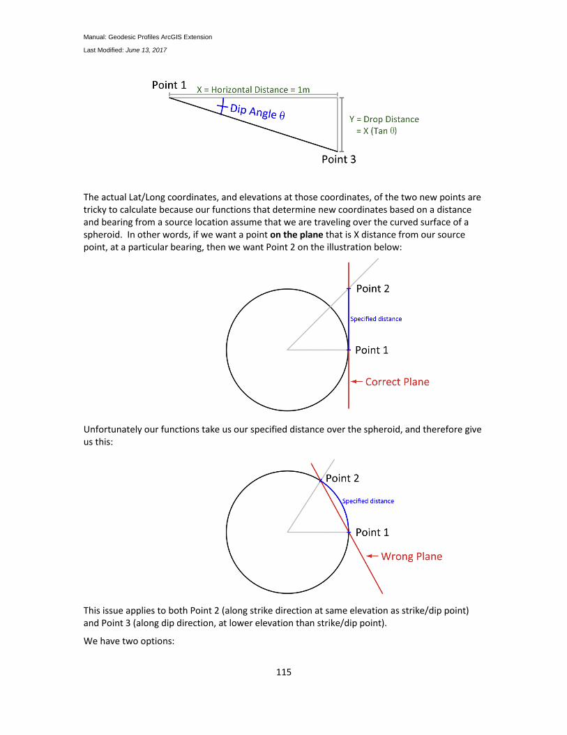
Manual: Geodesic Profiles ArcGIS Extension
Last Modified: June 13, 2017
115
The actual Lat/Long coordinates, and elevations at those coordinates, of the two new points are tricky to calculate because our functions that determine new coordinates based on a distance and bearing from a source location assume that we are traveling over the curved surface of a spheroid. In other words, if we want a point on the plane that is X distance from our source point, at a particular bearing, then we want Point 2 on the illustration below:
Unfortunately our functions take us our specified distance over the spheroid, and therefore give us this:
This issue applies to both Point 2 (along strike direction at same elevation as strike/dip point) and Point 3 (along dip direction, at lower elevation than strike/dip point).
We have two options:
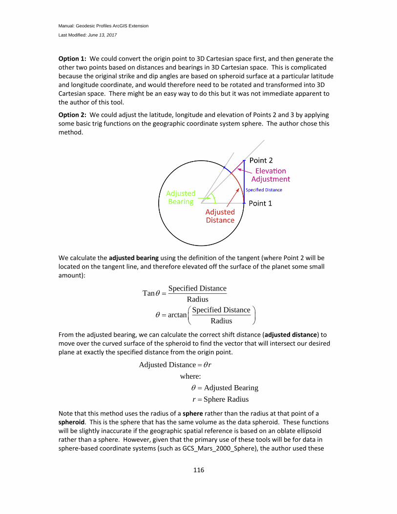
Manual: Geodesic Profiles ArcGIS Extension
Last Modified: June 13, 2017
116
Option 1: We could convert the origin point to 3D Cartesian space first, and then generate the other two points based on distances and bearings in 3D Cartesian space. This is complicated because the original strike and dip angles are based on spheroid surface at a particular latitude and longitude coordinate, and would therefore need to be rotated and transformed into 3D Cartesian space. There might be an easy way to do this but it was not immediate apparent to the author of this tool.
Option 2: We could adjust the latitude, longitude and elevation of Points 2 and 3 by applying some basic trig functions on the geographic coordinate system sphere. The author chose this method.
We calculate the adjusted bearing using the definition of the tangent (where Point 2 will be located on the tangent line, and therefore elevated off the surface of the planet some small amount):
Specified DistanceTan
Radius
Specified Distancearctan
Radius
From the adjusted bearing, we can calculate the correct shift distance (adjusted distance) to move over the curved surface of the spheroid to find the vector that will intersect our desired plane at exactly the specified distance from the origin point.
Adjusted Distance
where:
Adjusted Bearing
Sphere Radius
r
r
Note that this method uses the radius of a sphere rather than the radius at that point of a spheroid. This is the sphere that has the same volume as the data spheroid. These functions will be slightly inaccurate if the geographic spatial reference is based on an oblate ellipsoid rather than a sphere. However, given that the primary use of these tools will be for data in sphere-based coordinate systems (such as GCS_Mars_2000_Sphere), the author used these
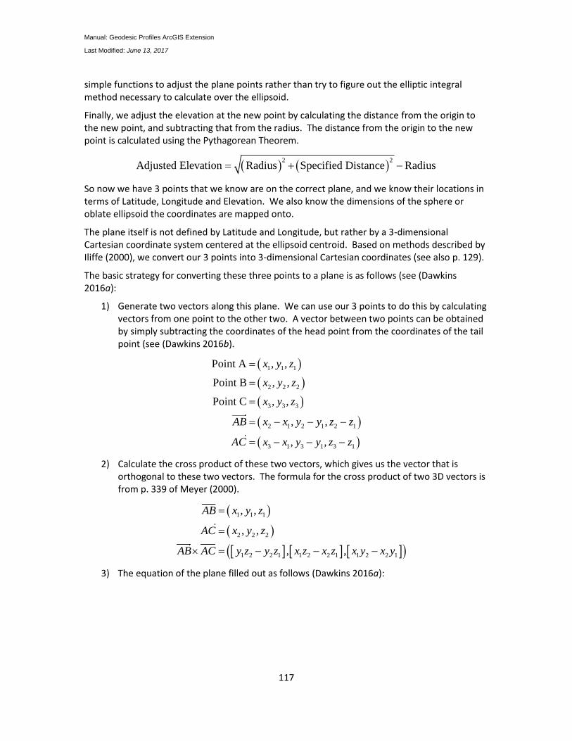
Manual: Geodesic Profiles ArcGIS Extension
Last Modified: June 13, 2017
117
simple functions to adjust the plane points rather than try to figure out the elliptic integral method necessary to calculate over the ellipsoid.
Finally, we adjust the elevation at the new point by calculating the distance from the origin to the new point, and subtracting that from the radius. The distance from the origin to the new point is calculated using the Pythagorean Theorem.
2 2
Adjusted Elevation Radius Specified Distance Radius
So now we have 3 points that we know are on the correct plane, and we know their locations in terms of Latitude, Longitude and Elevation. We also know the dimensions of the sphere or oblate ellipsoid the coordinates are mapped onto.
The plane itself is not defined by Latitude and Longitude, but rather by a 3-dimensional Cartesian coordinate system centered at the ellipsoid centroid. Based on methods described by Iliffe (2000), we convert our 3 points into 3-dimensional Cartesian coordinates (see also p. 129).
The basic strategy for converting these three points to a plane is as follows (see (Dawkins 2016a):
1) Generate two vectors along this plane. We can use our 3 points to do this by calculating vectors from one point to the other two. A vector between two points can be obtained by simply subtracting the coordinates of the head point from the coordinates of the tail point (see (Dawkins 2016b).
1 1 1
2 2 2
3 3 3
2 1 2 1 2 1
3 1 3 1 3 1
Point A , ,
Point B , ,
Point C , ,
, ,
, ,
x y z
x y z
x y z
AB x x y y z z
AC x x y y z z
2) Calculate the cross product of these two vectors, which gives us the vector that is orthogonal to these two vectors. The formula for the cross product of two 3D vectors is from p. 339 of Meyer (2000).
1 1 1
2 2 2
1 2 2 1 1 2 2 1 1 2 2 1
, ,
, ,
, ,
AB x y z
AC x y z
AB AC y z y z x z x z x y x y
3) The equation of the plane filled out as follows (Dawkins 2016a):
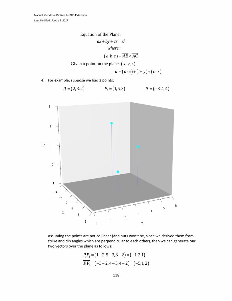
Manual: Geodesic Profiles ArcGIS Extension
Last Modified: June 13, 2017
118
Equation of the Plane:
:
, ,
Given a point on the plane : , ,
ax by cz d
where
a b c AB AC
x y z
d a x b y c z
4) For example, suppose we had 3 points:
1 2 12,3,2 1,5,3 3,4,4P P P
Assuming the points are not collinear (and ours won’t be, since we derived them from strike and dip angles which are perpendicular to each other), then we can generate our two vectors over the plane as follows:
1 2
1 3
1 2,5 3,3 2 1,2,1
3 2,4 3,4 2 5,1,2
PP
PP
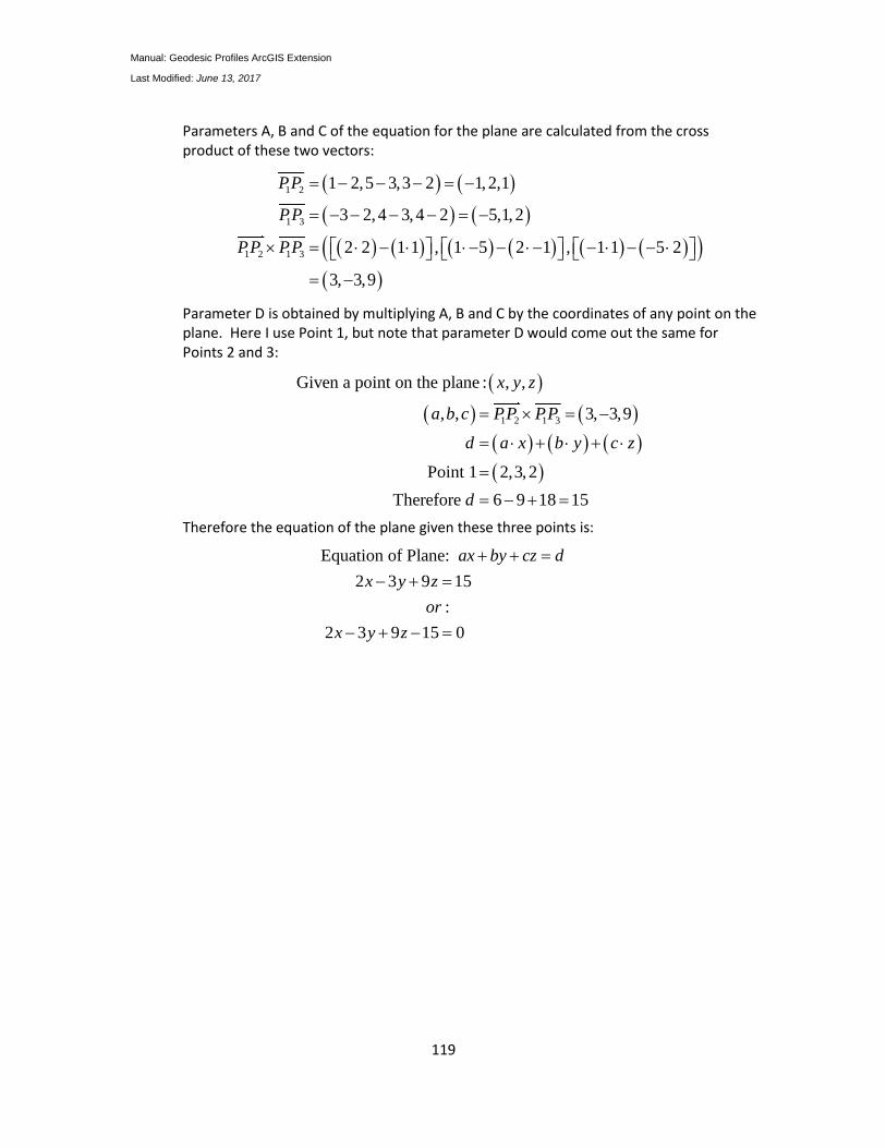
Manual: Geodesic Profiles ArcGIS Extension
Last Modified: June 13, 2017
119
Parameters A, B and C of the equation for the plane are calculated from the cross product of these two vectors:
1 2
1 3
1 2 1 3
1 2,5 3,3 2 1,2,1
3 2, 4 3,4 2 5,1, 2
2 2 1 1 , 1 5 2 1 , 1 1 5 2
3, 3,9
PP
PP
PP PP
Parameter D is obtained by multiplying A, B and C by the coordinates of any point on the plane. Here I use Point 1, but note that parameter D would come out the same for Points 2 and 3:
1 2 1 3
Given a point on the plane : , ,
, , 3, 3,9
Point 1 2,3,2
Therefore 6 9 18 15
x y z
a b c PP PP
d a x b y c z
d
Therefore the equation of the plane given these three points is:
Equation of Plane:
2 3 9 15
:
2 3 9 15 0
ax by cz d
x y z
or
x y z
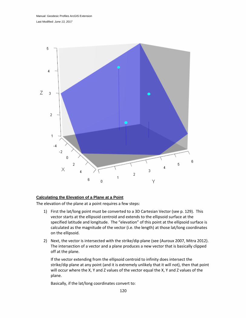
Manual: Geodesic Profiles ArcGIS Extension
Last Modified: June 13, 2017
120
Calculating the Elevation of a Plane at a Point
The elevation of the plane at a point requires a few steps:
1) First the lat/long point must be converted to a 3D Cartesian Vector (see p. 129). This vector starts at the ellipsoid centroid and extends to the ellipsoid surface at the specified latitude and longitude. The “elevation” of this point at the ellipsoid surface is calculated as the magnitude of the vector (i.e. the length) at those lat/long coordinates on the ellipsoid.
2) Next, the vector is intersected with the strike/dip plane (see (Auroux 2007, Mitra 2012). The intersection of a vector and a plane produces a new vector that is basically clipped off at the plane.
If the vector extending from the ellipsoid centroid to infinity does intersect the strike/dip plane at any point (and it is extremely unlikely that it will not), then that point will occur where the X, Y and Z values of the vector equal the X, Y and Z values of the plane.
Basically, if the lat/long coordinates convert to:
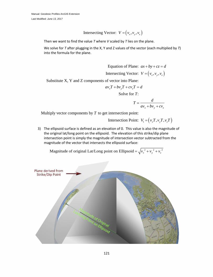
Manual: Geodesic Profiles ArcGIS Extension
Last Modified: June 13, 2017
121
Intersecting Vector: , ,x y zV v v v
Then we want to find the value T where V scaled by T lies on the plane.
We solve for T after plugging in the X, Y and Z values of the vector (each multiplied by T) into the formula for the plane.
Equation of Plane:
Intersecting Vector: , ,
Substitute X, Y and Z components of vector into Plane:
Solve for :
Multiply vector components by to get int
x y z
x y z
x y z
ax by cz d
V v v v
av T bv T cv T d
T
dT
av bv cv
T
1
ersection point:
Intersection Point: , ,x y zV v T v T v T
3) The ellipsoid surface is defined as an elevation of 0. This value is also the magnitude of the original lat/long point on the ellipsoid. The elevation of this strike/dip plane intersection point is simply the magnitude of intersection vector subtracted from the magnitude of the vector that intersects the ellipsoid surface:
2 2 2Magnitude of original Lat/Long point on Ellipsoid x y zv v v
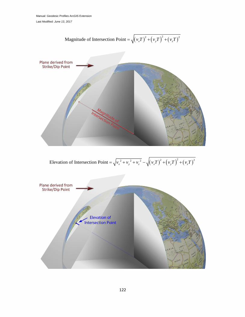
Manual: Geodesic Profiles ArcGIS Extension
Last Modified: June 13, 2017
122
22 2
Magnitude of Intersection Point x y zv T v T v T
22 22 2 2Elevation of Intersection Point x y z x y zv v v v T v T v T
Manual: Geodesic Profiles ArcGIS Extension
Last Modified: June 13, 2017
123
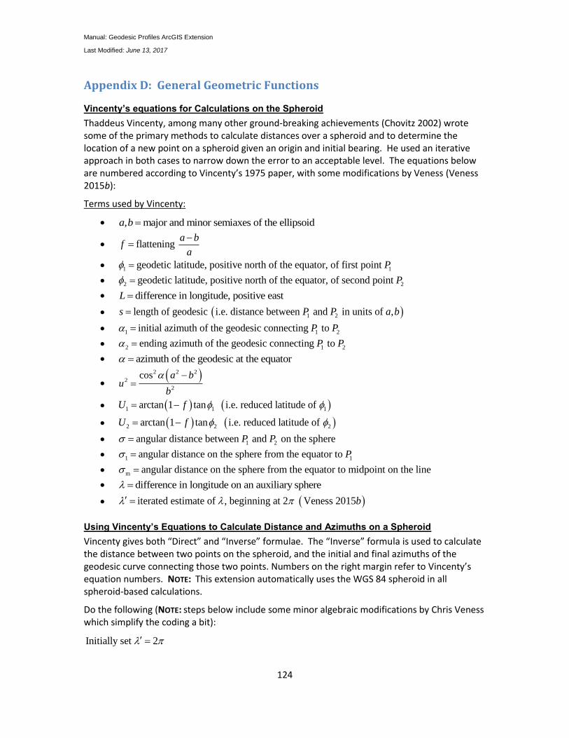
Manual: Geodesic Profiles ArcGIS Extension
Last Modified: June 13, 2017
124
Appendix D: General Geometric Functions
Vincenty’s equations for Calculations on the Spheroid
Thaddeus Vincenty, among many other ground-breaking achievements (Chovitz 2002) wrote some of the primary methods to calculate distances over a spheroid and to determine the location of a new point on a spheroid given an origin and initial bearing. He used an iterative approach in both cases to narrow down the error to an acceptable level. The equations below are numbered according to Vincenty’s 1975 paper, with some modifications by Veness (Veness 2015b):
Terms used by Vincenty:
, major and minor semiaxes of the ellipsoida b
flattening a b
fa
1 1geodetic latitude, positive north of the equator, of first point P
2 2geodetic latitude, positive north of the equator, of second point P
difference in longitude, positive eastL
1 2length of geodesic i.e. distance between and in units of ,s P P a b
1 1 2initial azimuth of the geodesic connecting to P P
2 1 2ending azimuth of the geodesic connecting to P P
azimuth of the geodesic at the equator
2 2 2
2
2
cos a bu
b
1 1 1arctan 1 tan i.e. reduced latitude of U f
2 2 2arctan 1 tan i.e. reduced latitude of U f
1 2angular distance between and on the sphereP P
1 1angular distance on the sphere from the equator to P
m angular distance on the sphere from the equator to midpoint on the line
difference in longitude on an auxiliary sphere
iterated estimate of , beginning at 2 Veness 2015b
Using Vincenty’s Equations to Calculate Distance and Azimuths on a Spheroid
Vincenty gives both “Direct” and “Inverse” formulae. The “Inverse” formula is used to calculate the distance between two points on the spheroid, and the initial and final azimuths of the geodesic curve connecting those two points. Numbers on the right margin refer to Vincenty’s equation numbers. NOTE: This extension automatically uses the WGS 84 spheroid in all spheroid-based calculations.
Do the following (NOTE: steps below include some minor algebraic modifications by Chris Veness which simplify the coding a bit):
Initially set 2
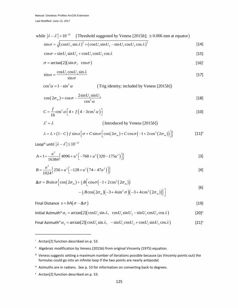
Manual: Geodesic Profiles ArcGIS Extension
Last Modified: June 13, 2017
125
12while 10 Threshold suggested by Veness [2015 ]; 0.006 mm at equatorb
2 2
2 1 2 1 2 sin cos sin cos sin sin cos cosU U U U U [14]
1 2 1 2 cos sin sin cos cos cosU U U U [15]
arctan[2] sin , cos [16]i
1 2cos cos sin sin
sin
U U
[17]
2 2 cos 1 sin Trig identity; included by Veness [2015 ]b
1 2
2
2sin sin cos 2 cos
cosm
U U
[18]
2 2 cos 4 4 3cos16
fC f
[10]
Introduced by Veness [2015 ]b
2 1 sin sin cos 2 cos 1 2cos 2m mL C f C C
[11]ii
Loopiii until 1210
2
2 2 21 4096 768 320 17516384
uA u u u
[3]
2
2 2 2256 128 74 471024
uB u u u
[4]
214
2 216
sin cos 2 cos 1 2cos 2
cos 2 3 4sin 3 4cos 2
m m
m m
B B
B
[6]
Final Distance s bA [19]
Initial Azimuthiv 1 2 1 2 1 2arctan[2] cos sin , cos sin sin cos cosU U U U U [20]v
Final Azimuthiv 2 1 1 2 1 2arctan[2] cos sin , sin cos cos sin cosU U U U U [21]v
i Arctan[2] function described on p. 53.
ii Algebraic modification by Veness (2015b) from original Vincenty (1975) equation.
iii Veness suggests setting a maximum number of iterations possible because (as Vincenty points out) the formulas could go into an infinite loop if the two points are nearly antipodal.
iv Azimuths are in radians. See p. 53 for information on converting back to degrees.
v Arctan[2] function described on p. 53.
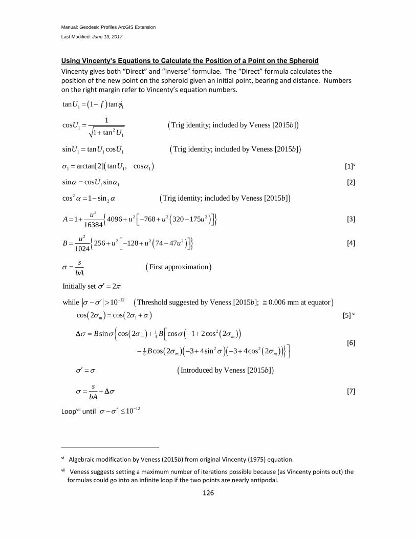
Manual: Geodesic Profiles ArcGIS Extension
Last Modified: June 13, 2017
126
Using Vincenty’s Equations to Calculate the Position of a Point on the Spheroid
Vincenty gives both “Direct” and “Inverse” formulae. The “Direct” formula calculates the position of the new point on the spheroid given an initial point, bearing and distance. Numbers on the right margin refer to Vincenty’s equation numbers.
1 1tan 1 tanU f
12
1
1cos Trig identity; included by Veness [2015 ]
1 tanU b
U
1 1 1sin tan cos Trig identity; included by Veness [2015 ]U U U b
1 1 1arctan[2] tan , cosU [1]v
1 1sin cos sinU [2]
2
2cos 1 sin Trig identity; included by Veness [2015 ]b
2
2 2 21 4096 768 320 17516384
uA u u u
[3]
2
2 2 2256 128 74 471024
uB u u u
[4]
First approximations
bA
Initially set 2
12while 10 Threshold suggested by Veness [2015 ]; 0.006 mm at equatorb
1 cos 2 cos 2m [5] vi
214
2 216
sin cos 2 cos 1 2cos 2
cos 2 3 4sin 3 4cos 2
m m
m m
B B
B
[6]
Introduced by Veness [2015 ]b
s
bA [7]
Loopvii until 1210
vi Algebraic modification by Veness (2015b) from original Vincenty (1975) equation.
vii Veness suggests setting a maximum number of iterations possible because (as Vincenty points out) the formulas could go into an infinite loop if the two points are nearly antipodal.
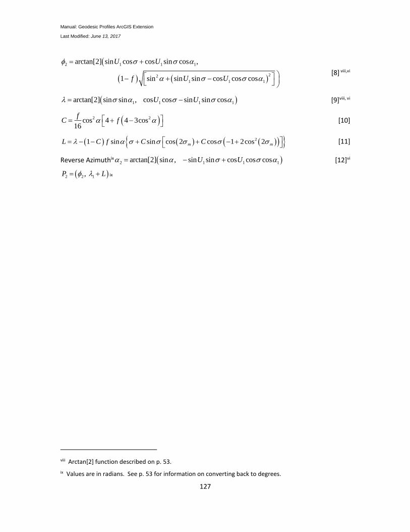
Manual: Geodesic Profiles ArcGIS Extension
Last Modified: June 13, 2017
127
2 1 1 1
22
1 1 1
arctan[2] sin cos cos sin cos ,
1 sin sin sin cos cos cos
U U
f U U
[8] viii,vi
1 1 1 1arctan[2] sin sin , cos cos sin sin cosU U [9]viii, vi
2 2cos 4 4 3cos16
fC f
[10]
21 sin sin cos 2 cos 1 2cos 2m mL C f C C
[11]
Reverse Azimuthix 2 1 1 1arctan[2] sin , sin sin cos cos cosU U [12]vi
2 2 1, P L ix
viii Arctan[2] function described on p. 53.
ix Values are in radians. See p. 53 for information on converting back to degrees.
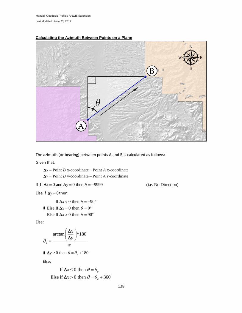
Manual: Geodesic Profiles ArcGIS Extension
Last Modified: June 13, 2017
128
Calculating the Azimuth Between Points on a Plane
The azimuth (or bearing) between points A and B is calculated as follows:
Given that:
Point x-coordinate Point x-coordinate
Point y-coordinate Point y-coordinate
x B A
y B A
If If 0 and 0 then 9999 (i.e. No Direction)x y
Else if 0y then:
If
If 0 then 90º
Else If 0 then 0º
Else If 0 then 90º
x
x
x
Else:
arctan *180
a
x
y
If 0 then 180ay
Else:
If 0 then
Else if 0 then 360
a
a
x
x
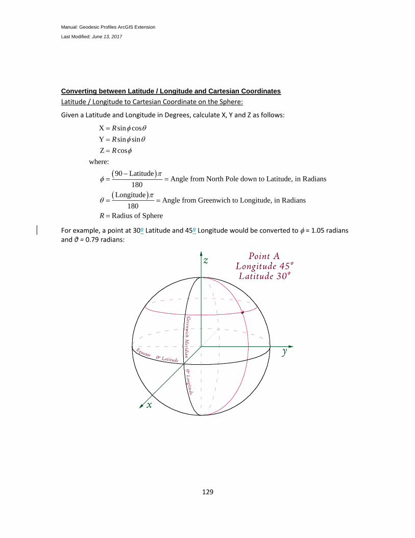
Manual: Geodesic Profiles ArcGIS Extension
Last Modified: June 13, 2017
129
Converting between Latitude / Longitude and Cartesian Coordinates
Latitude / Longitude to Cartesian Coordinate on the Sphere:
Given a Latitude and Longitude in Degrees, calculate X, Y and Z as follows:
X sin cos
Y sin sin
Z cos
where:
90 LatitudeAngle from North Pole down to Latitude, in Radians
180
LongitudeAngle from Greenwich to Longitude, in Radians
180
Radius of Sphere
R
R
R
R
For example, a point at 30º Latitude and 45º Longitude would be converted to = 1.05 radians and θ = 0.79 radians:
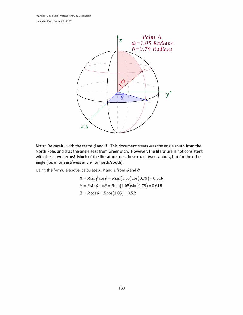
Manual: Geodesic Profiles ArcGIS Extension
Last Modified: June 13, 2017
130
NOTE: Be careful with the terms and θ! This document treats as the angle south from the North Pole, and θ as the angle east from Greenwich. However, the literature is not consistent with these two terms! Much of the literature uses these exact two symbols, but for the other
angle (i.e. for east/west and θ for north/south).
Using the formula above, calculate X, Y and Z from and θ.
X sin cos sin 1.05 cos 0.79 0.61
Y sin sin sin 1.05 sin 0.79 0.61
Z cos cos 1.05 0.5
R R R
R R R
R R R
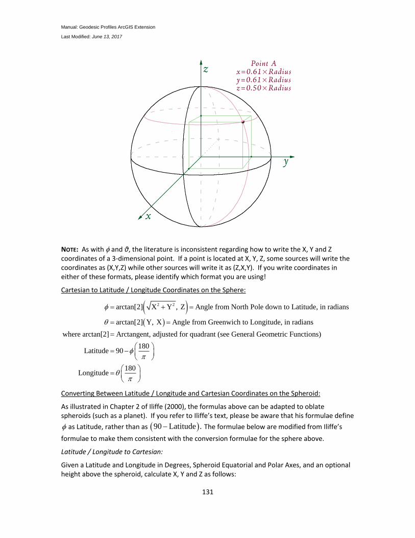
Manual: Geodesic Profiles ArcGIS Extension
Last Modified: June 13, 2017
131
NOTE: As with and θ, the literature is inconsistent regarding how to write the X, Y and Z coordinates of a 3-dimensional point. If a point is located at X, Y, Z, some sources will write the coordinates as (X,Y,Z) while other sources will write it as (Z,X,Y). If you write coordinates in either of these formats, please identify which format you are using!
Cartesian to Latitude / Longitude Coordinates on the Sphere:
2 2arctan[2] X Y , Z Angle from North Pole down to Latitude, in radians
arctan[2] Y, X Angle from Greenwich to Longitude, in radians
where arctan[2] Arctangent, adjusted for quadrant (see General Geomet
ric Functions)
180Latitude 90
180Longitude
Converting Between Latitude / Longitude and Cartesian Coordinates on the Spheroid:
As illustrated in Chapter 2 of Iliffe (2000), the formulas above can be adapted to oblate spheroids (such as a planet). If you refer to Iliffe’s text, please be aware that his formulae define
as Latitude, rather than as 90 Latitude . The formulae below are modified from Iliffe’s
formulae to make them consistent with the conversion formulae for the sphere above.
Latitude / Longitude to Cartesian:
Given a Latitude and Longitude in Degrees, Spheroid Equatorial and Polar Axes, and an optional height above the spheroid, calculate X, Y and Z as follows:
Manual: Geodesic Profiles ArcGIS Extension
Last Modified: June 13, 2017
132
2
X sin cos
Y sin sin
Z 1 cos
where:
90 LatitudeAngle from North Pole down to Latitude, in Radians
180
LongitudeAngle from Greenwich to Longitude, in Radians
180
Spheroid equatorial radi
h
h
e h
a
2 22
2
2 2
us (i.e. semi-major axis)
Spheroid polar radius (i.e. semi-minor axis)
-Spheroid eccentricity (squared)
1 cos
Height aove the spheroid
b
a be
a
a
e
h
Cartesian to Latitude / Longitude Coordinates on the Spheroid:
2 3 3
180Latitude 90
180Longitude
where:
arctan[2] cos , Z+ sin Angle from North Pole down to Latitude, in radians
arctan[2] Y, X Angle from Greenwich to Longitude, in radians
Sphe
P e a u b u
a
2 2
2 22
2
2
2
roid equatorial radius (i.e. semi-major axis)
Spheroid polar radius (i.e. semi-minor axis)
X Y
arctan[2] Z ,
-Spheroid eccentricity (squared)
1
arctan[2] Arctangent, adjusted for
b
P
u a Pb
a be
a
e
e
quadrant (see General Geometric Functions)
Manual: Geodesic Profiles ArcGIS Extension
Last Modified: June 13, 2017
133
Arctan[2] Function
Various functions in this extension calculate arctangents. However, there is a problem with the basic function arctan because it does not account for quadrant. For example, given that
tanY
AX
, then
.arctan
YA
X
, where A is in radians. However, this simple arctan function
does not properly account for the signs of X and Y and will only return values ranging
between 2
. The arctan[2] function checks the signs of X and Y and returns a value of A
radians that correctly ranges from to .
Unfortunately, Visual Basic 6 does not have a function to calculate arctangent in this manner. Many programming languages such as C++, PHP, C# and VB.NET include the “atan2” function which does the trick. You simply specify X and Y separately and the function determines the quadrant. NOTE: Microsoft Excel also has an “atan2” function, but for some reason the Excel version takes the X and Y values in the order of (x, y) while all other implementations in the civilized world appear to take these values in the order of (y, x). Therefore be careful if you use this function in both your code and in Excel!
Given the lack of an Atan2 function in VB6 and VBA, I wrote my own function as follows:
Const dblPi As Double = 3.14159265358979
Public Function atan2(Y As Double, X As Double) As Double
If X > 0 Then
atan2 = Atn(Y / X)
ElseIf X < 0 Then
If Y = 0 Then
atan2 = (dblPi - Atn(Abs(Y / X)))
Else
atan2 = Sgn(Y) * (dblPi - Atn(Abs(Y / X)))
End If
Else ' IF X = 0
If Y = 0 Then
atan2 = 0
Else
atan2 = Sgn(Y) * dblPi / 2
End If
End If
End Function
Converting between Radians and Decimal Degrees
Radians clockwise from North180
180Degrees clockwise from North
Degrees
Radians
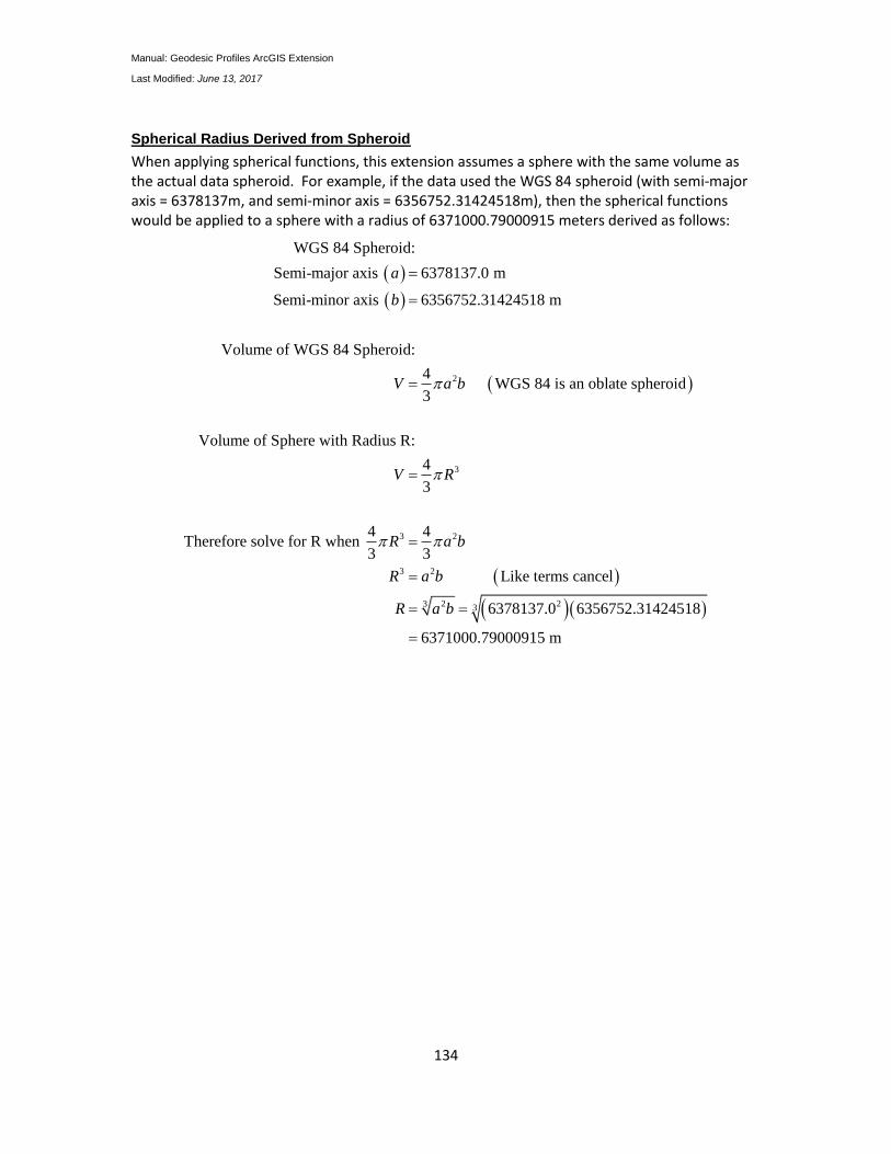
Manual: Geodesic Profiles ArcGIS Extension
Last Modified: June 13, 2017
134
Spherical Radius Derived from Spheroid
When applying spherical functions, this extension assumes a sphere with the same volume as the actual data spheroid. For example, if the data used the WGS 84 spheroid (with semi-major axis = 6378137m, and semi-minor axis = 6356752.31424518m), then the spherical functions would be applied to a sphere with a radius of 6371000.79000915 meters derived as follows:
2
3
WGS 84 Spheroid:
Semi-major axis 6378137.0 m
Semi-minor axis 6356752.31424518 m
Volume of WGS 84 Spheroid:
4 WGS 84 is an oblate spheroid
3
Volume of Sphere with Radius R:
4
3
Therefore solv
a
b
V a b
V R
3 2
3 2
2 23 3
4 4e for R when
3 3
Like terms cancel
6378137.0 6356752.31424518
6371000.79000915 m
R a b
R a b
R a b
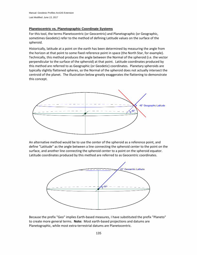
Manual: Geodesic Profiles ArcGIS Extension
Last Modified: June 13, 2017
135
Planetocentric vs. Planetographic Coordinate Systems
For this tool, the terms Planetocentric (or Geocentric) and Planetographic (or Geographic, sometimes Geodetic) refer to the method of defining Latitude values on the surface of the spheroid.
Historically, latitude at a point on the earth has been determined by measuring the angle from the horizon at that point to some fixed reference point in space (the North Star, for example). Technically, this method produces the angle between the Normal of the spheroid (i.e. the vector perpendicular to the surface of the spheroid) at that point. Latitude coordinates produced by this method are referred to as Geographic (or Geodetic) coordinates. Planetary spheroids are typically slightly flattened spheres, so the Normal of the spheroid does not actually intersect the centroid of the planet. The illustration below greatly exaggerates the flattening to demonstrate this concept.
An alternative method would be to use the center of the spheroid as a reference point, and define "Latitude" as the angle between a line connecting the spheroid center to the point on the surface, and another line connecting the spheroid center to a point on the spheroid equator. Latitude coordinates produced by this method are referred to as Geocentric coordinates.
Because the prefix "Geo" implies Earth-based measures, I have substituted the prefix "Planeto" to create more general terms. Note: Most earth-based projections and datums are Planetographic, while most extra-terrestrial datums are Planetocentric.
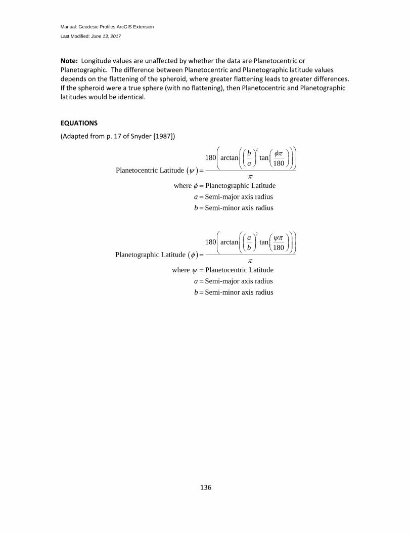
Manual: Geodesic Profiles ArcGIS Extension
Last Modified: June 13, 2017
136
Note: Longitude values are unaffected by whether the data are Planetocentric or Planetographic. The difference between Planetocentric and Planetographic latitude values depends on the flattening of the spheroid, where greater flattening leads to greater differences. If the spheroid were a true sphere (with no flattening), then Planetocentric and Planetographic latitudes would be identical.
EQUATIONS
(Adapted from p. 17 of Snyder [1987])
2
180 arctan tan180
Planetocentric Latitude
where Planetographic Latitude
Semi-major axis radius
Semi-minor axis radius
b
a
a
b
2
180 arctan tan180
Planetographic Latitude
where Planetocentric Latitude
Semi-major axis radius
Semi-minor axis radius
a
b
a
b
Manual: Geodesic Profiles ArcGIS Extension
Last Modified: June 13, 2017
137
Analyzing Directional Data: Circular Statistics
Before beginning this section, I want to emphasize two important points that people very often make mistakes with:
1) Do not calculate the mean direction using the arithmetic mean! This is especially frustrating because the arithmetic mean is sometimes correct and sometimes wildly incorrect. For example, the mean direction of 90° and 180° is 135°, which coincidentally
is equal to the arithmetic mean90
1352
. But what is the mean direction of
359° and 1°? They are both pointing almost due north (± 1°), and clearly the true mean direction is exactly due north. However, the arithmetic mean gives us 180°
359180
2
, which is due south and exactly the opposite of the correct answer. The
correct way to calculate the mean direction is described below.
2) If you apply a Sine or Cosine transformation, make sure to convert the values to radians first! Most analytical software and programming languages have sine and cosine functions, but these functions usually assume the values are in radians, not degrees. There are exactly 2π (~6.28) radians in a circle. This means that the software will assume that a difference of 3.14 (i.e. π) units is equivalent to going halfway around the circle. If your data are in degrees, then the software will interpret a change in 2° to be roughly equivalent to going a third of the way around the circle. Fortunately it is easy to convert to radians using the following formula:
3 14159265358979
180 180
.DegreesDegreesRadians
Degrees to Radians:
It is possible that your software has a function that allows you to calculate sines and cosines from degrees (many calculators do), but even in this case you must remember to set the switch correctly.
Fortunately there are well-established methods available for analyzing circular or periodic data such as movement direction or aspect. The circular nature of the data lead to very specific and interesting approaches to calculating measures of central tendency and dispersion (see also (Jenness 2015). Some of the basic descriptive statistics are:
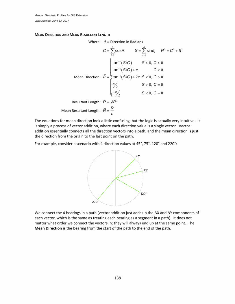
Manual: Geodesic Profiles ArcGIS Extension
Last Modified: June 13, 2017
138
MEAN DIRECTION AND MEAN RESULTANT LENGTH
2 2 2
1 1
1
1
1
2
0 0
0
2 0 0
0 02
0 02
cos sin
tan ,
tan
tan ,
,
,
n n
i i
i i
C S R C S
S C S C
S C C
S C S C
S C
S C
R R
Where: Direction in Radians
Mean Direction:
Resultant Length:
Mean Resultant LenR
Rn
gth:
The equations for mean direction look a little confusing, but the logic is actually very intuitive. It is simply a process of vector addition, where each direction value is a single vector. Vector addition essentially connects all the direction vectors into a path, and the mean direction is just the direction from the origin to the last point on the path.
For example, consider a scenario with 4 direction values at 45°, 75°, 120° and 220°:
We connect the 4 bearings in a path (vector addition just adds up the ∆X and ∆Y components of each vector, which is the same as treating each bearing as a segment in a path). It does not matter what order we connect the vectors in; they will always end up at the same point. The Mean Direction is the bearing from the start of the path to the end of the path.
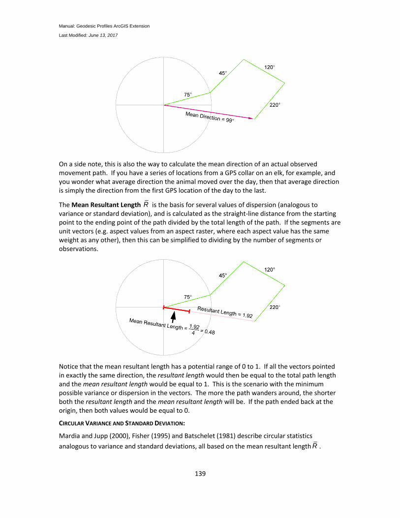
Manual: Geodesic Profiles ArcGIS Extension
Last Modified: June 13, 2017
139
On a side note, this is also the way to calculate the mean direction of an actual observed movement path. If you have a series of locations from a GPS collar on an elk, for example, and you wonder what average direction the animal moved over the day, then that average direction is simply the direction from the first GPS location of the day to the last.
The Mean Resultant Length R is the basis for several values of dispersion (analogous to variance or standard deviation), and is calculated as the straight-line distance from the starting point to the ending point of the path divided by the total length of the path. If the segments are unit vectors (e.g. aspect values from an aspect raster, where each aspect value has the same weight as any other), then this can be simplified to dividing by the number of segments or observations.
Notice that the mean resultant length has a potential range of 0 to 1. If all the vectors pointed in exactly the same direction, the resultant length would then be equal to the total path length and the mean resultant length would be equal to 1. This is the scenario with the minimum possible variance or dispersion in the vectors. The more the path wanders around, the shorter both the resultant length and the mean resultant length will be. If the path ended back at the origin, then both values would be equal to 0.
CIRCULAR VARIANCE AND STANDARD DEVIATION:
Mardia and Jupp (2000), Fisher (1995) and Batschelet (1981) describe circular statistics
analogous to variance and standard deviations, all based on the mean resultant length R .
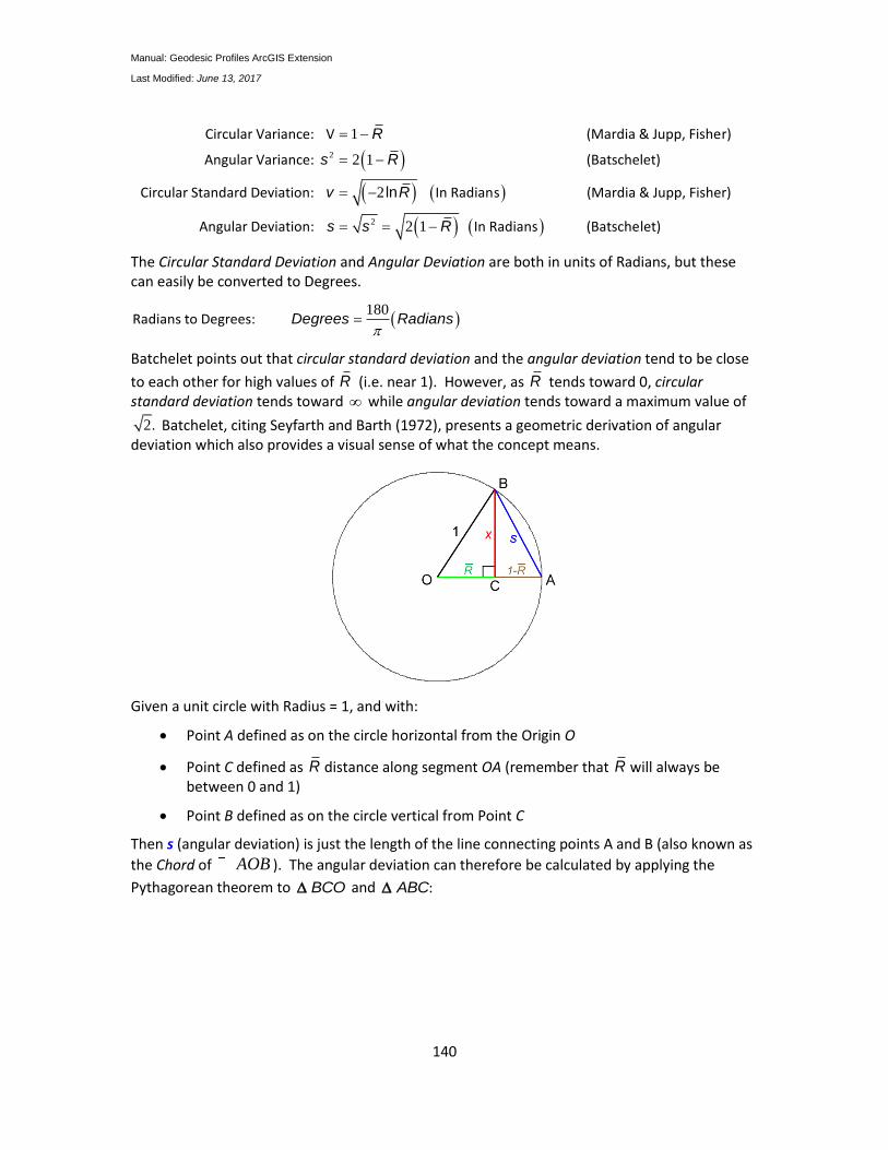
Manual: Geodesic Profiles ArcGIS Extension
Last Modified: June 13, 2017
140
2
2
1
2 1
2
2 1
Circular Variance: V (Mardia & Jupp, Fisher)
Angular Variance: (Batschelet)
Circular Standard Deviation: In Radians (Mardia & Jupp, Fisher)
Angular Deviation: In Radians (Batsche
ln
R
s R
v R
s s R let)
The Circular Standard Deviation and Angular Deviation are both in units of Radians, but these can easily be converted to Degrees.
180
Degrees Radians
Radians to Degrees:
Batchelet points out that circular standard deviation and the angular deviation tend to be close
to each other for high values of R (i.e. near 1). However, as R tends toward 0, circular standard deviation tends toward while angular deviation tends toward a maximum value of
2. Batchelet, citing Seyfarth and Barth (1972), presents a geometric derivation of angular deviation which also provides a visual sense of what the concept means.
Given a unit circle with Radius = 1, and with:
Point A defined as on the circle horizontal from the Origin O
Point C defined as R distance along segment OA (remember that R will always be between 0 and 1)
Point B defined as on the circle vertical from Point C
Then s (angular deviation) is just the length of the line connecting points A and B (also known as
the Chord of AOB ). The angular deviation can therefore be calculated by applying the
Pythagorean theorem to BCO and :ABC
Manual: Geodesic Profiles ArcGIS Extension
Last Modified: June 13, 2017
141
2 2 2
2 2
22 2
2
22 2
2
2 2
1
1
1
1
1
1 1 1
1 2 1
2 2
2 1
2 1
:
:
:
BCO
AB
R
R
R
C
R R R
R R
Rs
s
s
R
R
R
R
x
x
x
x
R
From the Pythagorean Theorem on
From the Pythagorean Theorem on
Substituting for
Based on this illustration, it is easy to see that 0s when 1R , and that 2s when 0R
Note: A mean resultant length R near 1 always implies a tightly focused set of directions, but
a mean resultant length near 0 does not necessarily imply a high amount of variation or dispersion. All it implies is that the directions balance each other out. This can occur with a uniform distribution of directions, in which case there truly would be high dispersion. It can also occur, however, if you have a number of bearings in one direction and an equal number in the opposite direction. For example, perhaps you have a bird with distinct and separate roost and forage locations. Every day the bird travels to the forage location and then returns to the roost location. In this scenario, the bird only goes in two distinct and opposite directions (to the forage location, and then back to the roost location). The bird’s movement directions are highly focused and predictable, but the mean resultant length would be 0 and consequently the variance would be high. As with most situations, plotting the distribution of the data is a good way to understand what is really happening.
Just as with standard statistics, there are a number of circular distributions and sophisticated analytical techniques available. These go beyond the scope of this discussion, but please refer to (Jammalamadaka and SenGupta 2001), Mardia and Jupp (2000), Zar (1999; see especially ch. 26 and 27), Fisher (1995) and Batschelet (1981) for some good texts on circular statistics, distributions (i.e. the Fisher, Von Mises and Wrapped Normal distributions), circular hypothesis testing and other analytical techniques. There is also a good circular statistical package for R, originally based on Jammalamadaka and SenGupta’s text. As of June, 2016, the manual for this package can be viewed at http://cran.wustl.edu/web/packages/circular/circular.pdf.