multivariate and propensity score matching software with...
TRANSCRIPT
JSS Journal of Statistical SoftwareMay 2011, Volume 42, Issue 7. http://www.jstatsoft.org/
Multivariate and Propensity Score Matching
Software with Automated Balance Optimization:
The Matching Package for R
Jasjeet S. SekhonUC Berkeley
Abstract
Matching is an R package which provides functions for multivariate and propensityscore matching and for finding optimal covariate balance based on a genetic search algo-rithm. A variety of univariate and multivariate metrics to determine if balance actuallyhas been obtained are provided. The underlying matching algorithm is written in C++,makes extensive use of system BLAS and scales efficiently with dataset size. The geneticalgorithm which finds optimal balance is parallelized and can make use of multiple CPUsor a cluster of computers. A large number of options are provided which control exactlyhow the matching is conducted and how balance is evaluated.
Keywords: propensity score matching, multivariate matching, genetic optimization, causalinference, R.
1. Introduction
The R (R Development Core Team 2011) package Matching implements a variety of algo-rithms for multivariate matching including propensity score, Mahalanobis, inverse varianceand genetic matching (GenMatch). The last of these, genetic matching, is a method whichautomatically finds the set of matches which minimize the discrepancy between the distri-bution of potential confounders in the treated and control groups—i.e., covariate balanceis maximized. The package enables a wide variety of matching options including matchingwith or without replacement, bias adjustment, different methods for handling ties, exact andcaliper matching, and a method for the user to fine tune the matches via a general restrictionmatrix. Variance estimators include the usual Neyman standard errors (which condition onthe matched data), Abadie and Imbens (2006) standard errors which account for the (asymp-

2 Matching: Multivariate Matching with Automated Balance Optimization in R
totic) variance induced by the matching procedure itself, and robust variances which do notassume a homogeneous causal effect. The Matching software package is available from theComprehensive R Archive Network at http://CRAN.R-project.org/package=Matching.
The package provides a set of functions to do the matching (Match) and to evaluate how goodcovariate balance is before and after matching (MatchBalance). The GenMatch function findsoptimal balance using multivariate matching where a genetic search algorithm determines theweight each covariate is given. Balance is determined by examining cumulative probabilitydistribution functions of a variety of standardized statistics. By default, these statistics in-clude paired t tests, univariate and multivariate Kolmogorov-Smirnov (KS) tests. A variety ofdescriptive statistics based on empirical-QQ plots are also offered. The statistics are not usedto conduct formal hypothesis tests, because no measure of balance is a monotonic functionof bias in the estimand of interest and because we wish to maximize balance without limit.GenMatch can maximize balance based on a variety of pre-defined loss functions or any lossfunction the user may wish to provide.
In the next section I briefly offer some background material on both the Rubin causal modeland matching methods. Section 3 provides an overview of the Matching package with exam-ples. Section 4 concludes.
2. Background on matching
Matching has become an increasingly popular method of causal inference in many fieldsincluding statistics (Rubin 2006; Rosenbaum 2002), medicine (Christakis and Iwashyna 2003;Rubin 1997), economics (Abadie and Imbens 2006; Dehejia and Wahba 2002, 1999), politicalscience (Bowers and Hansen 2005; Herron and Wand 2007; Imai 2005), sociology (Morganand Harding 2006; Diprete and Engelhardt 2004; Winship and Morgan 1999; Smith 1997)and even law (Rubin 2001). There is, however, no consensus on how exactly matching oughtto be done and how to measure the success of the matching procedure. A wide variety ofmatching procedures have been proposed, and Matching implements many of them.
When using matching methods to estimate causal effects, a central problem is deciding howbest to perform the matching. Two common approaches are propensity score matching(Rosenbaum and Rubin 1983) and multivariate matching based on Mahalanobis distance(Cochran and Rubin 1973; Rubin 1979, 1980). Matching methods based on the propensityscore (estimated by logistic regression), Mahalanobis distance or a combination of the two haveappealing theoretical properties if covariates have ellipsoidal distributions—e.g., distributionssuch as the normal or t. If the covariates are so distributed, these methods (more generallyaffinely invariant matching methods1) have the property of “equal percent bias reduction”(EPBR) (Rubin 1976a,b; Rubin and Thomas 1992).2 This property is formally defined inAppendix A. When this property holds, matching will reduce bias in all linear combinationsof the covariates. If the EPBR property does not hold, then, in general, matching will increasethe bias of some linear functions of the covariates even if all univariate means are closer inthe matched data than the unmatched (Rubin 1976a). Unfortunately, the EPBR property
1Affine invariance means that the matching output is invariant to matching on X or an affine transformationof X.
2The EPBR results of Rubin and Thomas (1992) have been extended by Rubin and Stuart (2006) to thecase of discriminant mixtures of proportional ellipsoidally symmetric (DMPES) distributions. This extensionis important, but it is restricted to a limited set of mixtures.
Journal of Statistical Software 3
rarely holds with actual data.
A significant shortcoming of common matching methods such as Mahalanobis distance andpropensity score matching is that they may (and in practice, frequently do) make balanceworse across measured potential confounders. These methods may make balance worse, inpractice, even if covariates are distributed ellipsoidally because in a given finite sample theremay be departures from an ellipsoidal distribution. Moreover, if covariates are neither el-lipsoidally symmetric nor are mixtures of discriminant mixtures of proportional ellipsoidallysymmetric (DMPES) distributions, propensity score matching has good theoretical propertiesif and only if the true propensity score model is known and the sample size is large.
These limitations often surprise applied researchers. Because of the limited theoretical prop-erties for matching when the propensity score is not known, one approach is to algorithmicallyimpose additional properties, and this is the approach used by genetic matching.
Diamond and Sekhon (2005) and Sekhon and Grieve (2011) propose a matching algorithm,genetic matching (GenMatch), that maximizes the balance of observed covariates betweentreated and control groups. GenMatch is a generalization of propensity score and Maha-lanobis distance matching, and it has been used by a variety of researchers (e.g., Andam,Ferraro, Pfaff, Sanchez-Azofeifa, and Robalino 2008; Eggers and Hainmueller 2009; Gilliganand Sergenti 2008; Gordon 2009; Heinrich 2007; Hopkins 2010; Morgan and Harding 2006;Lenz and Ladd 2009; Raessler and Rubin 2005). The algorithm uses a genetic algorithm(Mebane, Jr. and Sekhon 2011; Sekhon and Mebane 1998) to optimize balance as much aspossible given the data. The method is nonparametric and does not depend on knowingor estimating the propensity score, but the method is improved when a propensity score isincorporated.
The core motivation for all matching methods is the Rubin causal model which I discuss nextfollowed by details on Mahalanobis, propensity score and genetic matching.
2.1. Rubin causal model
The Rubin causal model conceptualizes causal inference in terms of potential outcomes undertreatment and control, only one of which is observed for each unit (Holland 1986; Splawa-Neyman 1923; Rubin 1974, 1978, 1990). A causal effect is defined as the difference betweenan observed outcome and its counterfactual.
Let Yi1 denote the potential outcome for unit i if the unit receives treatment, and let Yi0denote the potential outcome for unit i in the control regime. The treatment effect forobservation i is defined by τi = Yi1− Yi0. Causal inference is a missing data problem becauseYi1 and Yi0 are never both observed. Let Ti be a treatment indicator equal to 1 when i isin the treatment regime and 0 otherwise. The observed outcome for observation i is thenYi = TiYi1 + (1− Ti)Yi0.In principle, if assignment to treatment is randomized, causal inference is straightforwardbecause the two groups are drawn from the same population by construction, and treatmentassignment is independent of all baseline variables. As the sample size grows, observed andunobserved baseline variables are balanced across treatment and control groups with arbitrar-ily high probability, because treatment assignment is independent of Y0 and Y1—i.e., followingthe notation of Dawid (1979), {Yi0, Yi1 ⊥⊥ Ti}. Hence, for j = 0, 1
E(Yij | Ti = 1) = E(Yij | Ti = 0) = E(Yi | Ti = j)

4 Matching: Multivariate Matching with Automated Balance Optimization in R
Therefore, the average treatment effect (ATE) can be estimated by:
τ = E(Yi1 | Ti = 1)− E(Yi0 | Ti = 0)
= E(Yi | Ti = 1)− E(Yi | Ti = 0) (1)
Equation 1 is estimable in an experimental setting because observations in treatment andcontrol groups are exchangeable.3 In the simplest experimental setup, individuals in bothgroups are equally likely to receive the treatment, and hence assignment to treatment will notbe associated with the outcome. Even in an experimental setup, much can go wrong whichrequires statistical correction (e.g., Barnard, Frangakis, Hill, and Rubin 2003).
In an observational setting, covariates are almost never balanced across treatment and controlgroups because the two groups are not ordinarily drawn from the same population. Thus, acommon quantity of interest is the average treatment effect for the treated (ATT):
τ | (T = 1) = E(Yi1 | Ti = 1)− E(Yi0 | Ti = 1). (2)
Equation 2 cannot be directly estimated because Yi0 is not observed for the treated. Progresscan be made by assuming that selection into treatment depends on observable covariates X.Following Rosenbaum and Rubin (1983), one can assume that conditional on X, treatment as-signment is unconfounded ({Y0, Y1 ⊥⊥ T} | X) and that there is overlap: 0 < Pr(T = 1 | X) < 1.Together, unconfoundedness and overlap constitute a property known as strong ignorabilityof treatment assignment which is necessary for identifying the average treatment effect. Heck-man, Ichimura, Smith, and Todd (1998) show that for ATT, the unconfoundedness assumptioncan be weakened to mean independence: E (Yij | Ti, Xi) = E (Yij | Xi).
4 The overlap assump-tion for ATT only requires that the support of X for the treated be a subset of the supportof X for control observations.
Then, following Rubin (1974, 1977) we obtain
E(Yij | Xi, Ti = 1) = E(Yij | Xi, Ti = 0) = E(Yi | Xi, Ti = j). (3)
By conditioning on observed covariates, Xi, treatment and control groups are exchangeable.The average treatment effect for the treated is estimated as
τ | (T = 1) = E {E(Yi | Xi, Ti = 1)− E(Yi | Xi, Ti = 0) | Ti = 1} , (4)
where the outer expectation is taken over the distribution of Xi | (Ti = 1) which is thedistribution of baseline variables in the treated group.
The most straightforward and nonparametric way to condition on X is to exactly match onthe covariates. This is an old approach going back to at least Fechner (1966), the father ofpsychophysics. This approach fails in finite samples if the dimensionality of X is large or ifX contains continuous covariates. Thus, in general, alternative methods must be used.
3It is standard practice to assume the Stable Unit Treatment Value assumption, also known as SUTVA(Holland 1986; Rubin 1978). SUTVA requires that the treatment status of any unit be independent of potentialoutcomes for all other units, and that treatment is defined identically for all units.
4Also see Abadie and Imbens (2006).

Journal of Statistical Software 5
2.2. Mahalanobis and propensity score matching
The most common method of multivariate matching is based on Mahalanobis distance (Cochranand Rubin 1973; Rubin 1979, 1980). The Mahalanobis distance between any two column vec-tors is:
md(Xi, Xj) ={
(Xi −Xj)>S−1(Xi −Xj)
} 12
where S is the sample covariance matrix of X. To estimate ATT by matching with replace-ment, one matches each treated unit with the M closest control units, as defined by thisdistance measure, md().5 If X consists of more than one continuous variable, multivariatematching estimates contain a bias term which does not asymptotically go to zero at rate
√n
(Abadie and Imbens 2006).
An alternative way to condition on X is to match on the probability of assignment to treat-ment, known as the propensity score.6 As one’s sample size grows large, matching on thepropensity score produces balance on the vector of covariates X (Rosenbaum and Rubin1983).
Let e(Xi) ≡ Pr(Ti = 1 | Xi) = E(Ti | Xi), defining e(Xi) to be the propensity score. Given0 < Pr(Ti | Xi) < 1 and Pr(T1, T2, · · ·TN | X1, X2, · · ·XN ) = ΠN
i=1e(Xi)Ti(1 − e(Xi))
(1−Ti),Rosenbaum and Rubin (1983) prove that
τ | (T = 1) = E {E(Yi | e(Xi), Ti = 1)− E(Yi | e(Xi), Ti = 0) | Ti = 1} ,
where the outer expectation is taken over the distribution of e(Xi) | (Ti = 1). Since thepropensity score is generally unknown, it must be estimated.
Propensity score matching involves matching each treated unit to the nearest control unit onthe unidimensional metric of the propensity score vector. If the propensity score is estimatedby logistic regression, as is typically the case, much is to be gained by matching not on thepredicted probabilities (bounded between zero and one) but on the linear predictor µ̂ ≡ Xβ̂.Matching on the linear predictor avoids compression of propensity scores near zero and one.Moreover, the linear predictor is often more nearly normally distributed which is of someimportance given the EPBR results if the propensity score is matched on along with othercovariates.
Mahalanobis distance and propensity score matching can be combined in various ways (Ru-bin 2001; Rosenbaum and Rubin 1985). It is useful to combine the propensity score withMahalanobis distance matching because propensity score matching is particularly good atminimizing the discrepancy along the propensity score and Mahalanobis distance is particu-larly good at minimizing the distance between individual coordinates of X (orthogonal to thepropensity score) (Rosenbaum and Rubin 1985).
5Alternatively one can do optimal full matching (Hansen 2004; Hansen and Klopfer 2006; Rosenbaum 1989,1991) instead of the 1-to-N matching with replacement which I focus on in this article. This decision is aseparate one from the choice of a distance metric.
6The first estimator of treatment effects to be based on a weighted function of the probability of treatmentwas the Horvitz-Thompson statistic (Horvitz and Thompson 1952).

6 Matching: Multivariate Matching with Automated Balance Optimization in R
2.3. Genetic matching
The idea underlying the GenMatch algorithm is that if Mahalanobis distance is not optimal forachieving balance in a given dataset, one should be able to search over the space of distancemetrics and find something better. One way of generalizing the Mahalanobis metric is toinclude an additional weight matrix:
d(Xi, Xj) ={
(Xi −Xj)> (S−1/2)>WS−1/2(Xi −Xj)
} 12
where W is a k × k positive definite weight matrix and S1/2 is the Cholesky decompositionof S which is the variance-covariance matrix of X.7
Note that if one has a good propensity score model, one should include it as one of thecovariates in GenMatch. If this is done, both propensity score matching and Mahalanobismatching can be considered special limiting cases of GenMatch. If the propensity score containsall of the relevant information in a given sample, the other variables will be given zero weight.8
And GenMatch will converge to Mahalanobis distance if that proves to be the appropriatedistance measure.
GenMatch is an affinely invariant matching algorithm that uses the distance measure d(), inwhich all elements of W are zero except down the main diagonal. The main diagonal consistsof k parameters which must be chosen. Note that if each of these k parameters are set equalto 1, d() is the same as Mahalanobis distance.
The choice of setting the non-diagonal elements of W to zero is made for reasons of compu-tational power alone. The optimization problem grows exponentially with the number of freeparameters. It is important that the problem be parameterized so as to limit the number ofparameters which must be estimated.
This leaves the problem of how to choose the free elements of W . Many loss criteria recom-mend themselves, and GenMatch provides a number the user can choose from via the fit.funcand loss options of GenMatch. By default, cumulative probability distribution functions of avariety of standardized statistics are used as balance metrics and are optimized without limit.The default standardized statistics are paired t tests and nonparametric KS tests.
The statistics are not used to conduct formal hypothesis tests, because no measure of balanceis a monotonic function of bias in the estimand of interest and because we wish to maximizebalance without limit. Descriptive measures of discrepancy generally ignore key informationrelated to bias which is captured by probability distribution functions of standardized teststatistics. For example, using several descriptive metrics, one is unable to recover reliably theexperimental benchmark in a testbed dataset for matching estimators (Dehejia and Wahba1999). And these metrics, unlike those based on optimized distribution functions, performpoorly in a series of Monte Carlo sampling experiments just as one would expect given theirproperties. For details see Sekhon (2006a).
By default, GenMatch attempts to minimize a measure of the maximum observed discrepancybetween the matched treated and control covariates at every iteration of optimization. Fora given set of matches resulting from a given W , the loss is defined as the minimum p value
7The Cholesky decomposition is parameterized such that S = LL>, S1/2 = L. In other words, L is a lowertriangular matrix with positive diagonal elements.
8Technically, the other variables will be given weights just large enough to ensure that the weight matrix ispositive definite.
Journal of Statistical Software 7
observed across a series of standardized statistics. The user may specify exactly what testsare done via the BalanceMatrix option. Examples are offered in Section 3.
Conceptually, the algorithm attempts to minimize the largest observed covariate discrepancyat every step. This is accomplished by maximizing the smallest p value at each step.9 BecauseGenMatch is minimizing the maximum discrepancy observed at each step, it is minimizing theinfinity norm. This property holds even when, because of the distribution of X, the EPBRproperty does not hold. Therefore, if an analyst is concerned that matching may increasethe bias in some linear combination of X even if the means are reduced, GenMatch allowsthe analyst to put in the loss function all of the linear combinations of X which may be ofconcern. Indeed, any nonlinear function of X can also be included in the loss function, whichwould ensure that bias in some nonlinear functions of X is not made inordinately large bymatching.
The default GenMatch loss function does allow for imbalance in functions of X to worsen aslong as the maximum discrepancy is reduced. Hence, it is important that the maximum dis-crepancy be small—i.e., that the smallest p value be large. p values conventionally understoodto signal balance (e.g., 0.10), may be too low to produce reliable estimates. After GenMatchoptimization, the p values from these balance tests cannot be interpreted as true probabilitiesbecause of standard pre-test problems, but they remain useful measures of balance. Also,we are interested in maximizing the balance in the current sample so a hypothesis test forbalance is inappropriate.
The optimization problem described above is difficult and irregular, and the genetic algorithmimplemented in the rgenoud package (Mebane, Jr. and Sekhon 2011) is used to conduct theoptimization. Details of the algorithm are provided in Sekhon and Mebane (1998).
GenMatch is shown to have better properties than the usual alternative matching methodsboth when the EPBR property holds and when it does not (Sekhon 2006a; Diamond andSekhon 2005). Even when the EPBR property holds and the mapping from X to Y is lin-ear, GenMatch has better efficiency—i.e., lower mean square error (MSE)—in finite samples.When the EPBR property does not hold as it generally does not, GenMatch retains appeal-ing properties and the differences in performance between GenMatch and the other matchingmethods can become substantial both in terms of bias and MSE reduction. In short, at theexpense of computer time, GenMatch dominates the other matching methods in terms ofMSE when assumptions required for EPBR hold and, even more so, when they do not.
GenMatch is able to retain good properties even when EPBR does not hold because a set ofconstraints is imposed by the loss function optimized by the genetic algorithm. The loss func-tion depends on a large number of functions of covariate imbalance across matched treatmentand control groups. Given these measures, GenMatch will optimize covariate balance.
3. Package overview and examples
The three main functions in the package are Match, MatchBalance and GenMatch. The firstfunction, Match, performs multivariate and propensity score matching. It is intended to be
9More precisely lexical optimization will be done: all of the balance statistics will be sorted from the mostdiscrepant to the least and weights will be picked which minimize the maximum discrepancy. If multiple setsof weights result in the same maximum discrepancy, then the second largest discrepancy is examined to choosethe best weights. The processes continues iteratively until ties are broken.
8 Matching: Multivariate Matching with Automated Balance Optimization in R
used in conjunction with the MatchBalance function which checks if the results of Match haveactually achieved balance on a set of covariates. MatchBalance can also be used before anymatching to determine how balanced the raw data is. If one wants to do propensity scorematching, one should estimate the propensity model before calling Match, and then sendMatch the propensity score to use. The GenMatch function can be used to automatically findbalance by the use of a genetic search algorithm which determines the optimal weight to giveeach covariate.
Next, I present a set of propensity score (pscore) models which perform better as adjustmentsare made to them after the output of MatchBalance is examined. I then provide an exampleusing GenMatch.
3.1. Propensity score matching example
In order to do propensity score matching, the work flow is to first estimate a propensity scoreusing, for example, glm if one wants to estimate a propensity score using logistic regression. Anumber of alternative methods of estimating the propensity score, such as General AdditiveModels (GAMs), are possible. After the propensity score has been estimated, one calls Matchto perform the matching and MatchBalance to examine how well the matching procedure didin producing balance. If the balance results printed by MatchBalance are not good enough,one would go back and change either the propensity score model or some parameter of howthe matching is done—e.g., change from 1-to-3 matching to 1-to-1 matching.
The following example is adopted from the documentation of the Match function. The exampleuses the LaLonde (1986) experimental data which is based on a nationwide job trainingexperiment. The observations are individuals, and the outcome of interest is real earnings in1978. There are eight baseline variables age (age), years of education (educ), real earnings in1974 (re74), real earnings in 1975 (re75), and a series of indicator variables. The indicatorvariables are black (black), Hispanic (hisp), married (married) and lack of a high schooldiploma (nodegr).
R> library("Matching")
R> data("lalonde")
R> attach(lalonde)
Save the outcome of interest in Y and the treatment indicator in Tr:
R> Y <- lalonde$re78
R> Tr <- lalonde$treat
We now estimate our first propensity score model:
R> glm1 <- glm(Tr ~ age + educ + black + hisp + married + nodegr +
+ re74 + re75, family = binomial, data = lalonde)
Let us do one-to-one matching with replacement using our preliminary propensity score modelwhere the estimand is the average treatment effect on the treated (ATT):
R> rr1 <- Match(Y = Y, Tr = Tr, X = glm1$fitted)
Journal of Statistical Software 9
None of the forgoing commands produce output. If we wanted to see the results from the call toMatch which would display the estimate and its standard error we could do summary(rr1), butit is best to wait until we have achieved satisfactory balance before looking at the estimates.To this end, Match does not even need to be provided with an outcome variable—i.e., Y—inorder to work. Matches can be found and balance evaluated without knowledge of Y. Indeed,this is to be preferred so that the design stage of the observational study can be clearlyseparated from the estimation stage as is the case with experiments.
In the example above, the call to glm estimates a simple propensity score model and the syntaxof this procedure is covered in the R documentation. Then a call to Match is made which reliesheavily on the function’s default behavior because only three options are explicitly provided:a vector (Y) containing the outcome variable, a vector (Tr) containing the treatment status ofeach observation—i.e., either a zero or one—and a matrix (X) containing the variables to bematched on, which in this case is simply the propensity score. By default Match does 1-to-1matching with replacement and estimates ATT. The estimand is chosen via the estimand
option, as in estimand="ATE" to estimate the average treatment effect. The ratio of treatedto control observations is determined by the the M option and this ratio is by default set to 1.And whether matching should be done with replacement is controlled by the logical argumentreplace which defaults to TRUE for matching with replacement.
Ties are by default handled deterministically (Abadie and Imbens 2006) and this behavioris controlled by the ties option. By default ties = TRUE. If, for example, one treatedobservation matches more than one control observation, the matched dataset will include themultiple matched control observations and the matched data will be weighted to reflect themultiple matches. The sum of the weighted observations will still equal the original numberof observations. If ties = FALSE, ties will be randomly broken. This in general is not a goodidea because the variance of Y will be underestimated. But if the dataset is large and thereare many ties between potential matches, setting ties = FALSE often results in significantlyfaster execution with negligible bias. Whether two potential matches are close enough to beconsidered tied, is controlled by the distance.tolerance option.
With these defaults, the command
R> m1 = Match(Y = Y, Tr = Tr, X = glm1$fitted)
is equivalent to
R> m1 = Match(Y = Y, Tr = Tr, X = glm1$fitted, estimand = "ATT",
+ M = 1, ties = TRUE, replace = TRUE)
We generally want to measure balance for more functions of the data than we include inour propensity score model. We can do this using the following call to the MatchBalance
function. Note that the function is asked to measure balance for many more functions of theconfounders than we included in the propensity score model.
R> MatchBalance(Tr ~ age + I(age^2) + educ + I(educ^2) + black + hisp +
+ married + nodegr + re74 + I(re74^2) + re75 + I(re75^2) + u74 + u75 +
+ I(re74 * re75) + I(age * nodegr) + I(educ * re74) + I(educ * re75),
+ match.out = rr1, nboots = 1000, data = lalonde)
10 Matching: Multivariate Matching with Automated Balance Optimization in R
The full output for this call to MatchBalance is presented in Appendix B. The formula usedin the call to MatchBalance does not estimate any model. The formula is simply an efficientway to use the R modeling language to list the variables we wish to obtain univariate balancestatistics on. The dependent variable in the formula is the treatment indicator.
The propensity score model is different from the balance statistics which are requested fromMatchBalance. In general, one does not need to include all of the functions one wants totest balance on in the propensity score model. Indeed, doing so sometimes results in worsebalance. Generally, one should request balance statistics on more higher-order terms andinteractions than were included in the propensity score used to conduct the matching itself.
Aside from the formula, three additional arguments were given to the MatchBalance call.The match.out option is used to provide the output object from the previous call to Match.If this object is provided, MatchBalance will provide balance statistics for both before andafter matching, otherwise balance statistics will only be provided for the unmatched rawdataset. The nboots option determines the number of bootstrap samples to be run. If zero,no bootstraps are done. Bootstrapping is highly recommended because the bootstrappedKolmogorov-Smirnov test, unlike the standard test, provides correct coverage even when thereare point masses in the distributions being compared (Abadie 2002). At least 500 nboots
(preferably 1000) are recommended for publication quality p values. And finally, the data
argument expects a data frame which contains all of the variables in the formula. If a dataframe is not provided, the variables are obtained via lexical scoping.
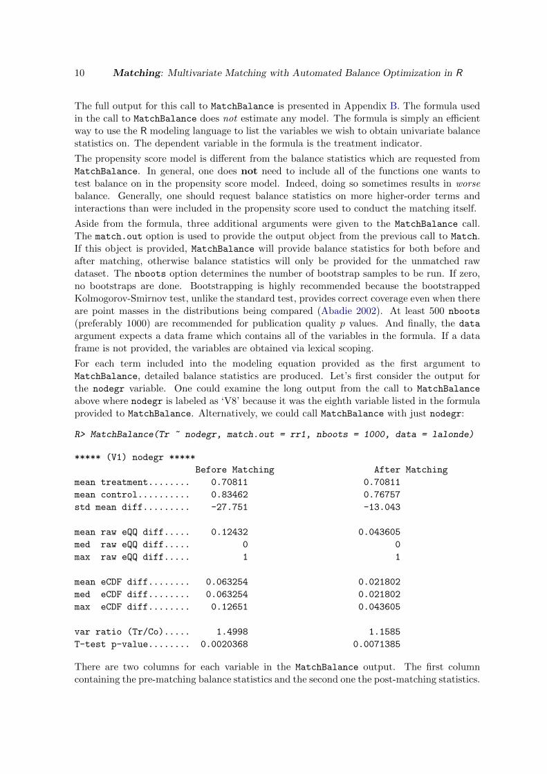
For each term included into the modeling equation provided as the first argument toMatchBalance, detailed balance statistics are produced. Let’s first consider the output forthe nodegr variable. One could examine the long output from the call to MatchBalance
above where nodegr is labeled as ‘V8’ because it was the eighth variable listed in the formulaprovided to MatchBalance. Alternatively, we could call MatchBalance with just nodegr:
R> MatchBalance(Tr ~ nodegr, match.out = rr1, nboots = 1000, data = lalonde)
***** (V1) nodegr *****
Before Matching After Matching
mean treatment........ 0.70811 0.70811
mean control.......... 0.83462 0.76757
std mean diff......... -27.751 -13.043
mean raw eQQ diff..... 0.12432 0.043605
med raw eQQ diff..... 0 0
max raw eQQ diff..... 1 1
mean eCDF diff........ 0.063254 0.021802
med eCDF diff........ 0.063254 0.021802
max eCDF diff........ 0.12651 0.043605
var ratio (Tr/Co)..... 1.4998 1.1585
T-test p-value........ 0.0020368 0.0071385
There are two columns for each variable in the MatchBalance output. The first columncontaining the pre-matching balance statistics and the second one the post-matching statistics.
Journal of Statistical Software 11
nodegr is an indicator variable for whether the individual in the worker training programhas a high school diploma. For such variables, the Kolmogorov-Smirnov test results are notpresented because they are the equivalent to the results from t tests.
Four different sets of balance statistics are provided for each variable. The first set consists ofthe means for the treatment and control groups. The second set contains summary statisticsbased on standardized empirical-QQ plots. The mean, median and maximum differencesin the standardized empirical-QQ plots are provided. The third set of statistics consists ofsummary statistics from the raw empirical-QQ plots so they are on the scale of the variablein question. And the last set of statistics provides the variance ratio of treatment over control(which should equal 1 if there is perfect balance), and the t test of difference of means (thepaired t test is provided post-matching). If they are calculated, the bootstrap Kolmogorov-Smirnov test results are also provided here.
The balance results make clear that nodegr is poorly balanced both before and after matching.Seventy-one percent of treatment observations have a high school diploma while seventy-sevenpercent of control observations do. And this difference is highly significant.
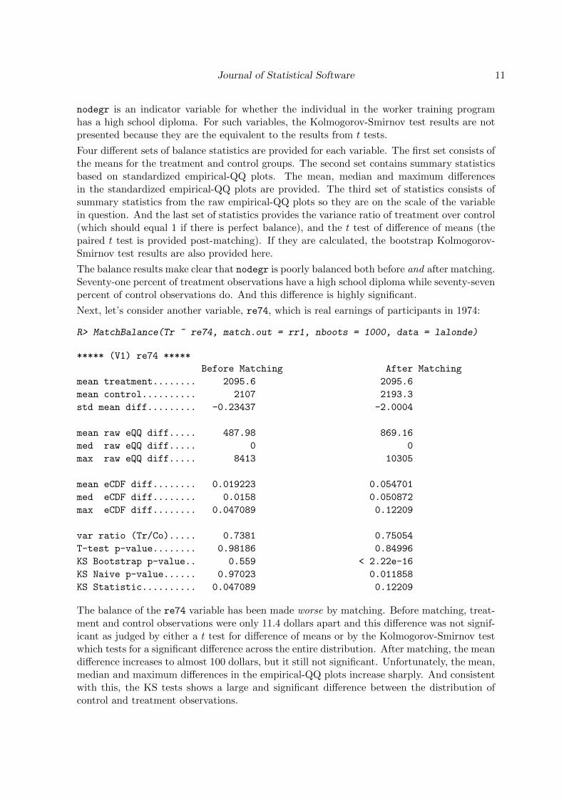
Next, let’s consider another variable, re74, which is real earnings of participants in 1974:
R> MatchBalance(Tr ~ re74, match.out = rr1, nboots = 1000, data = lalonde)
***** (V1) re74 *****
Before Matching After Matching
mean treatment........ 2095.6 2095.6
mean control.......... 2107 2193.3
std mean diff......... -0.23437 -2.0004
mean raw eQQ diff..... 487.98 869.16
med raw eQQ diff..... 0 0
max raw eQQ diff..... 8413 10305
mean eCDF diff........ 0.019223 0.054701
med eCDF diff........ 0.0158 0.050872
max eCDF diff........ 0.047089 0.12209
var ratio (Tr/Co)..... 0.7381 0.75054
T-test p-value........ 0.98186 0.84996
KS Bootstrap p-value.. 0.559 < 2.22e-16
KS Naive p-value...... 0.97023 0.011858
KS Statistic.......... 0.047089 0.12209
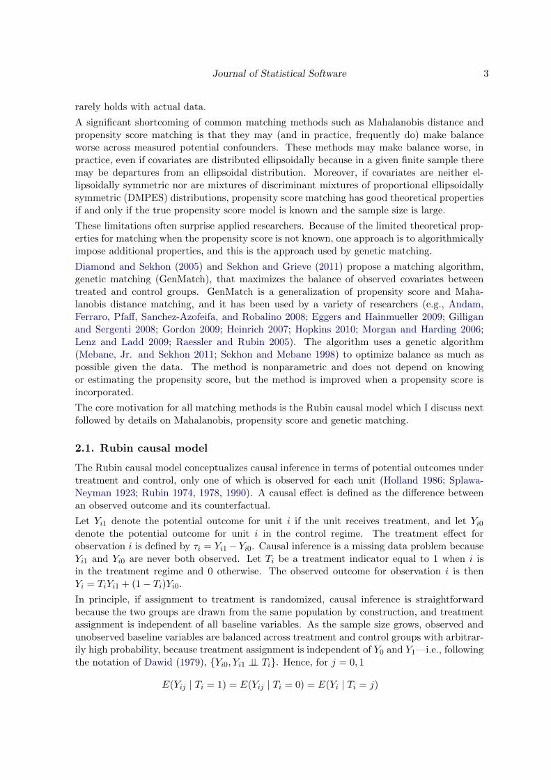
The balance of the re74 variable has been made worse by matching. Before matching, treat-ment and control observations were only 11.4 dollars apart and this difference was not signif-icant as judged by either a t test for difference of means or by the Kolmogorov-Smirnov testwhich tests for a significant difference across the entire distribution. After matching, the meandifference increases to almost 100 dollars, but it still not significant. Unfortunately, the mean,median and maximum differences in the empirical-QQ plots increase sharply. And consistentwith this, the KS tests shows a large and significant difference between the distribution ofcontrol and treatment observations.

12 Matching: Multivariate Matching with Automated Balance Optimization in R
●●●●●●●●●●●●●●●●●●●●●●●●●●●●●●●●●●●●●●●●●●●●●●●●●●●●●●●●●●●●●●●●●●●●●●●●●●●●●●●●●●●●●●●●●●●●●●●●●●●●●●●●●●●●●●●●●●●●●●●●●●●●●●●●●●●●●●●●●●●
●●●●●●●●●
●●●●●●
●●●●●●
●●●●●
●●●●●
●●●
●●●
● ● ●● ●
●
●
●
●
0 5000 10000 15000 20000 25000 30000 35000
050
0015
000
2500
035
000
Control Observations
Tre
atm
ent O
bser
vatio
ns
Before Matching
●●●●●●●●●●●●●●●●●●●●●●●●●●●●●●●●●●●●●●●●●●●●●●●●●●●●●●●●●●●●●●●●●●●●●●●●●●●●●●●●●●●●●●●●●●●●●●●●●●●●●●●●●●●●●●●●●●●●●●●●●●●●●●●●●●●●●●●●●●●●●●●●●●●●●●●●●●●●●●●●●●●●●●●●●●●●●●●●●●●●●●●●●●●●●●●●●●●●●●●●●●●●●●●●●●●●●●●●●●●●●●●●●●●●●●●●●●●●●●●●●●●●●●●●●●●●●●●●●●●●●●●●●●●●●●●●●●●●●●●●●●●●●
●●●●●●●●●●●●●●●●●●●●● ●●●
●●●● ●●●●●●● ●●
●●●●● ●● ●● ● ●
●●
●● ●●●
●
●
●
●
0 5000 10000 15000 20000 25000 30000 35000
050
0015
000
2500
035
000
Control Observations
Tre
atm
ent O
bser
vatio
ns
After Matching
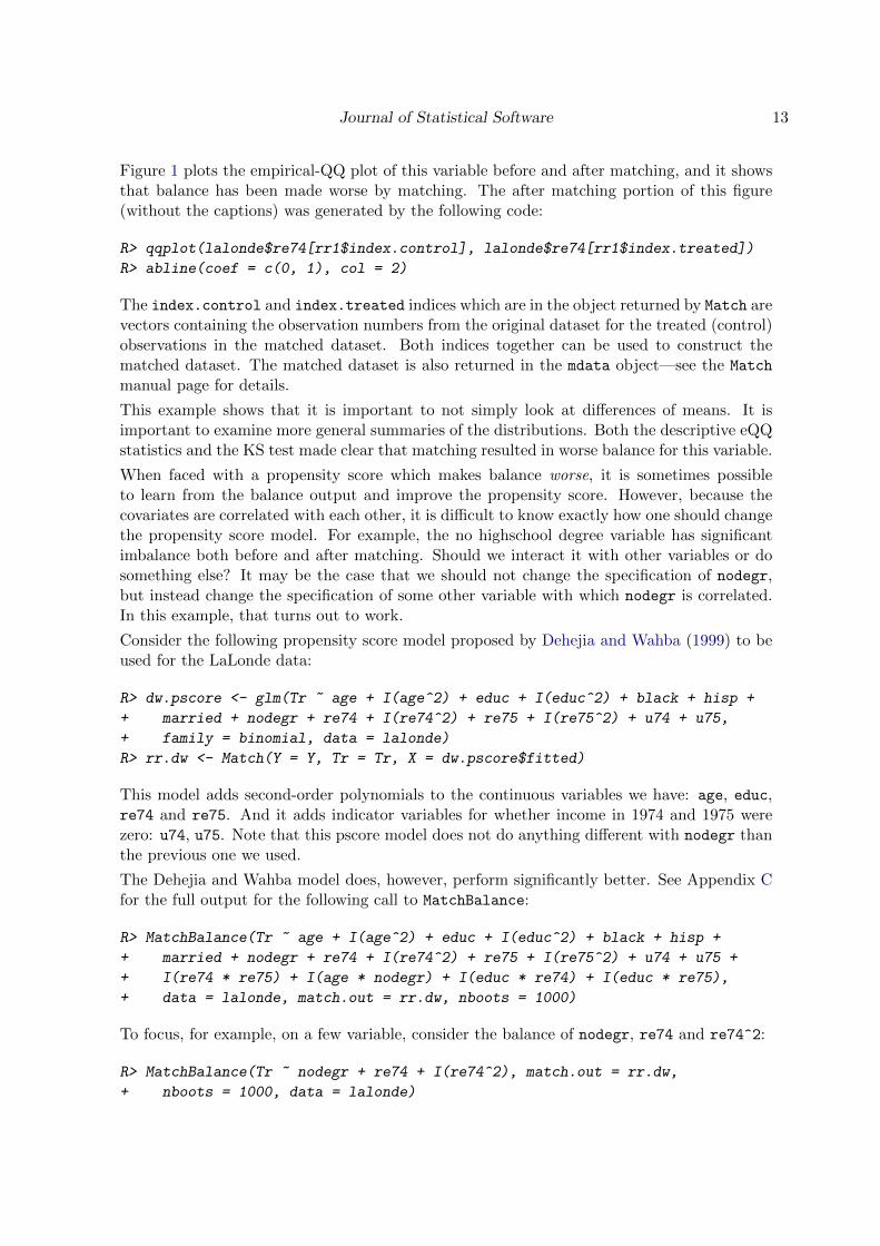
Figure 1: Empirical-QQ Plot of re74 before and after pscore matching.
Journal of Statistical Software 13
Figure 1 plots the empirical-QQ plot of this variable before and after matching, and it showsthat balance has been made worse by matching. The after matching portion of this figure(without the captions) was generated by the following code:
R> qqplot(lalonde$re74[rr1$index.control], lalonde$re74[rr1$index.treated])
R> abline(coef = c(0, 1), col = 2)
The index.control and index.treated indices which are in the object returned by Match arevectors containing the observation numbers from the original dataset for the treated (control)observations in the matched dataset. Both indices together can be used to construct thematched dataset. The matched dataset is also returned in the mdata object—see the Match
manual page for details.
This example shows that it is important to not simply look at differences of means. It isimportant to examine more general summaries of the distributions. Both the descriptive eQQstatistics and the KS test made clear that matching resulted in worse balance for this variable.
When faced with a propensity score which makes balance worse, it is sometimes possibleto learn from the balance output and improve the propensity score. However, because thecovariates are correlated with each other, it is difficult to know exactly how one should changethe propensity score model. For example, the no highschool degree variable has significantimbalance both before and after matching. Should we interact it with other variables or dosomething else? It may be the case that we should not change the specification of nodegr,but instead change the specification of some other variable with which nodegr is correlated.In this example, that turns out to work.
Consider the following propensity score model proposed by Dehejia and Wahba (1999) to beused for the LaLonde data:
R> dw.pscore <- glm(Tr ~ age + I(age^2) + educ + I(educ^2) + black + hisp +
+ married + nodegr + re74 + I(re74^2) + re75 + I(re75^2) + u74 + u75,
+ family = binomial, data = lalonde)
R> rr.dw <- Match(Y = Y, Tr = Tr, X = dw.pscore$fitted)
This model adds second-order polynomials to the continuous variables we have: age, educ,re74 and re75. And it adds indicator variables for whether income in 1974 and 1975 werezero: u74, u75. Note that this pscore model does not do anything different with nodegr thanthe previous one we used.
The Dehejia and Wahba model does, however, perform significantly better. See Appendix Cfor the full output for the following call to MatchBalance:
R> MatchBalance(Tr ~ age + I(age^2) + educ + I(educ^2) + black + hisp +
+ married + nodegr + re74 + I(re74^2) + re75 + I(re75^2) + u74 + u75 +
+ I(re74 * re75) + I(age * nodegr) + I(educ * re74) + I(educ * re75),
+ data = lalonde, match.out = rr.dw, nboots = 1000)
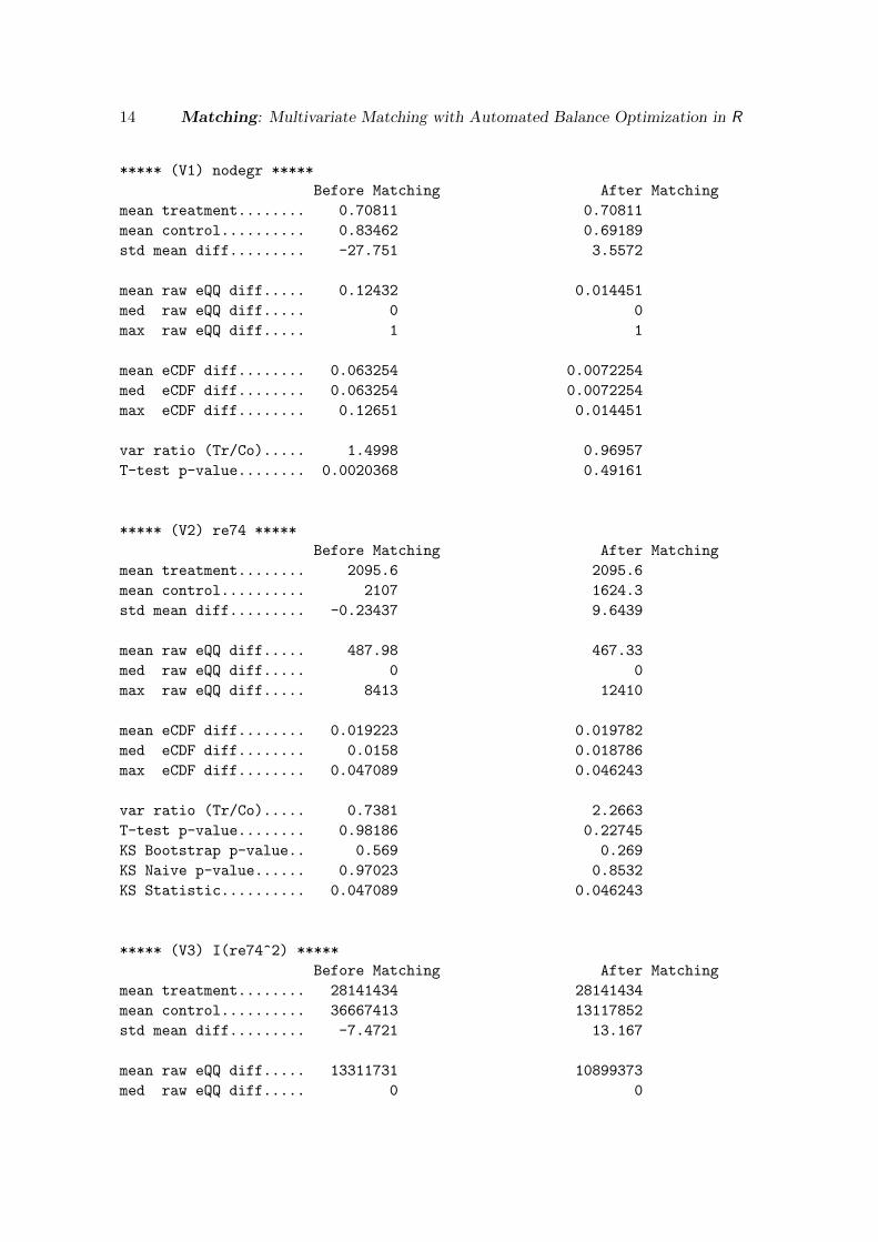
To focus, for example, on a few variable, consider the balance of nodegr, re74 and re74^2:
R> MatchBalance(Tr ~ nodegr + re74 + I(re74^2), match.out = rr.dw,
+ nboots = 1000, data = lalonde)
14 Matching: Multivariate Matching with Automated Balance Optimization in R
***** (V1) nodegr *****
Before Matching After Matching
mean treatment........ 0.70811 0.70811
mean control.......... 0.83462 0.69189
std mean diff......... -27.751 3.5572
mean raw eQQ diff..... 0.12432 0.014451
med raw eQQ diff..... 0 0
max raw eQQ diff..... 1 1
mean eCDF diff........ 0.063254 0.0072254
med eCDF diff........ 0.063254 0.0072254
max eCDF diff........ 0.12651 0.014451
var ratio (Tr/Co)..... 1.4998 0.96957
T-test p-value........ 0.0020368 0.49161
***** (V2) re74 *****
Before Matching After Matching
mean treatment........ 2095.6 2095.6
mean control.......... 2107 1624.3
std mean diff......... -0.23437 9.6439
mean raw eQQ diff..... 487.98 467.33
med raw eQQ diff..... 0 0
max raw eQQ diff..... 8413 12410
mean eCDF diff........ 0.019223 0.019782
med eCDF diff........ 0.0158 0.018786
max eCDF diff........ 0.047089 0.046243
var ratio (Tr/Co)..... 0.7381 2.2663
T-test p-value........ 0.98186 0.22745
KS Bootstrap p-value.. 0.569 0.269
KS Naive p-value...... 0.97023 0.8532
KS Statistic.......... 0.047089 0.046243
***** (V3) I(re74^2) *****
Before Matching After Matching
mean treatment........ 28141434 28141434
mean control.......... 36667413 13117852
std mean diff......... -7.4721 13.167
mean raw eQQ diff..... 13311731 10899373
med raw eQQ diff..... 0 0
Journal of Statistical Software 15
max raw eQQ diff..... 365146387 616156569
mean eCDF diff........ 0.019223 0.019782
med eCDF diff........ 0.0158 0.018786
max eCDF diff........ 0.047089 0.046243
var ratio (Tr/Co)..... 0.50382 7.9006
T-test p-value........ 0.51322 0.08604
KS Bootstrap p-value.. 0.569 0.269
KS Naive p-value...... 0.97023 0.8532
KS Statistic.......... 0.047089 0.046243
Before Matching Minimum p.value: 0.0020368
Variable Name(s): nodegr Number(s): 1
After Matching Minimum p.value: 0.08604
Variable Name(s): I(re74^2) Number(s): 3
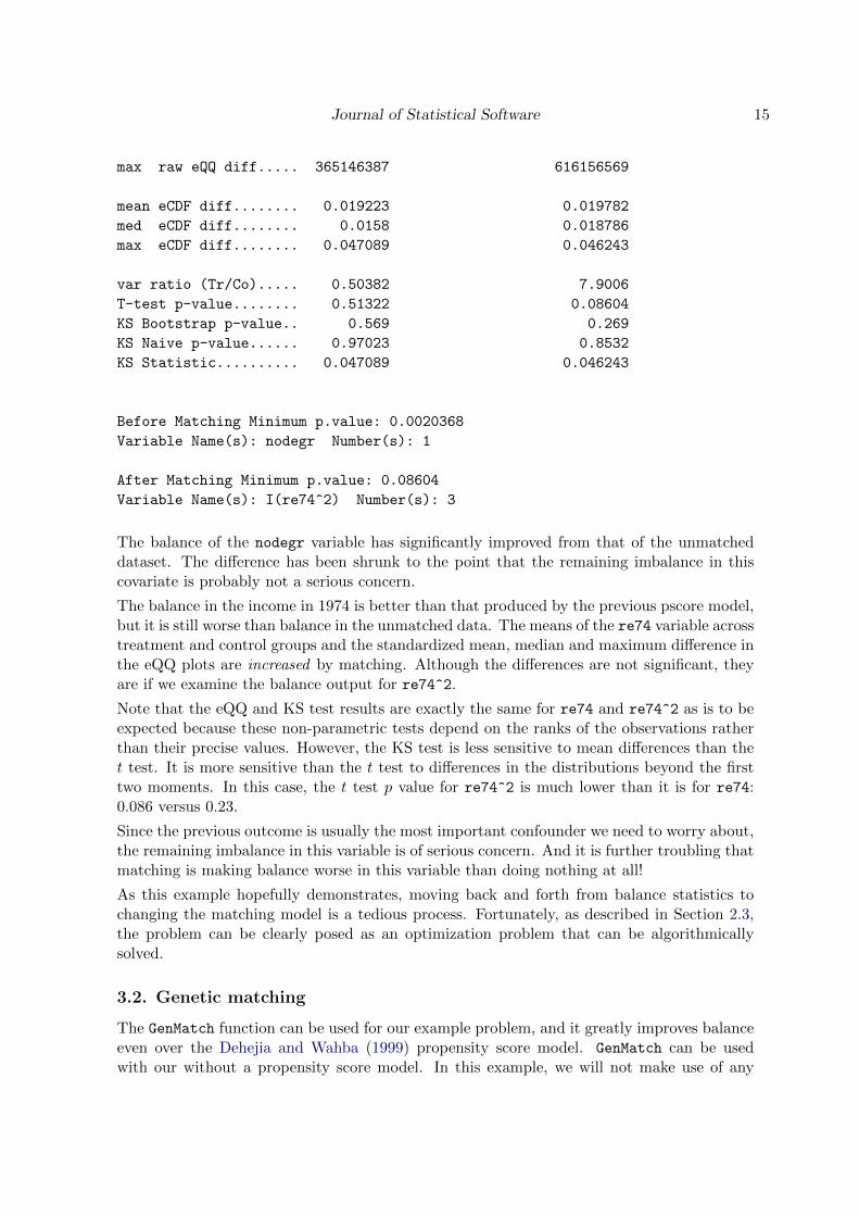
The balance of the nodegr variable has significantly improved from that of the unmatcheddataset. The difference has been shrunk to the point that the remaining imbalance in thiscovariate is probably not a serious concern.
The balance in the income in 1974 is better than that produced by the previous pscore model,but it is still worse than balance in the unmatched data. The means of the re74 variable acrosstreatment and control groups and the standardized mean, median and maximum difference inthe eQQ plots are increased by matching. Although the differences are not significant, theyare if we examine the balance output for re74^2.
Note that the eQQ and KS test results are exactly the same for re74 and re74^2 as is to beexpected because these non-parametric tests depend on the ranks of the observations ratherthan their precise values. However, the KS test is less sensitive to mean differences than thet test. It is more sensitive than the t test to differences in the distributions beyond the firsttwo moments. In this case, the t test p value for re74^2 is much lower than it is for re74:0.086 versus 0.23.
Since the previous outcome is usually the most important confounder we need to worry about,the remaining imbalance in this variable is of serious concern. And it is further troubling thatmatching is making balance worse in this variable than doing nothing at all!
As this example hopefully demonstrates, moving back and forth from balance statistics tochanging the matching model is a tedious process. Fortunately, as described in Section 2.3,the problem can be clearly posed as an optimization problem that can be algorithmicallysolved.
3.2. Genetic matching
The GenMatch function can be used for our example problem, and it greatly improves balanceeven over the Dehejia and Wahba (1999) propensity score model. GenMatch can be usedwith our without a propensity score model. In this example, we will not make use of any

16 Matching: Multivariate Matching with Automated Balance Optimization in R
propensity score model just to demonstrate that GenMatch can perform well even without ahuman providing such a model. However, in general, inclusion of a good propensity scoremodel helps GenMatch.
R> X <- cbind(age, educ, black, hisp, married, nodegr, re74, re75, u74, u75)
R> BalanceMatrix <- cbind(age, I(age^2), educ, I(educ^2), black, hisp,
+ married, nodegr, re74, I(re74^2), re75, I(re75^2), u74, u75,
+ I(re74 * re75), I(age * nodegr), I(educ * re74), I(educ * re75))
R> gen1 <- GenMatch(Tr = Tr, X = X, BalanceMatrix = BalanceMatrix,
+ pop.size = 1000)
GenMatch takes four key arguments. The first two, Tr and X, are just the same as those of theMatch function: the first is a vector for the treatment indicator and the second a matrix whichcontains the covariates which we wish to match on. The third key argument, BalanceMatrix,is a matrix containing the variables we wish to achieve balance on. This is by default equalto X, but it can be a matrix which contains more or less variables than X or variables whichare transformed in various ways. It should generally contain the variables and the functionof these variables that we wish to balance. In this example, I have made BalanceMatrix
contain the same terms we had MatchBalance test balance for, and this, in general, is goodpractice. If you care about balance for a given function of the covariates, you should put itin BalanceMatrix just like how you should put it into the equation in MatchBalance.
The pop.size argument is important and greatly influences how long the function takes torun. This argument controls the population size used by the evolutionary algorithm–i.e., itis the number of individuals genoud uses to solve the optimization problem. This argumentis also the number of random trail solutions which are tried at the beginning of the searchprocess. The theorems proving that genetic algorithms find good solutions are asymptotic inpopulation size. Therefore, it is important that this value not be small (Vose 1993; Nix andVose 1992). On the other hand, computational time is finite so obvious trade-offs must bemade.
GenMatch has a large number of other options which are detailed in its help page. The optionscontrolling features of the matching itself, such as whether to match with replacement, are thesame as those of the Match function. But many other options are specific to GenMatch becausethey control the optimization process. The most important of these aside from pop.size, arewait.generations and max.generations.
In order to obtain balance statistics, we can simply do the following with the output object(gen1) returned by the call to GenMatch above:
R> mgen1 <- Match(Y = Y, Tr = Tr, X = X, Weight.matrix = gen1)
R> MatchBalance(Tr ~ age + I(age^2) + educ + I(educ^2) + black + hisp +
+ married + nodegr + re74 + I(re74^2) + re75 + I(re75^2) + u74 + u75 +
+ I(re74 * re75) + I(age * nodegr) + I(educ * re74) + I(educ * re75),
+ data = lalonde, match.out = mgen1, nboots = 1000)
The balance results from this GenMatch run are excellent. The full output from this call toMatchBalance is include in Appendix D. Note that GenMatch is a stochastic algorithm soyour results may not be exactly the same.
Journal of Statistical Software 17
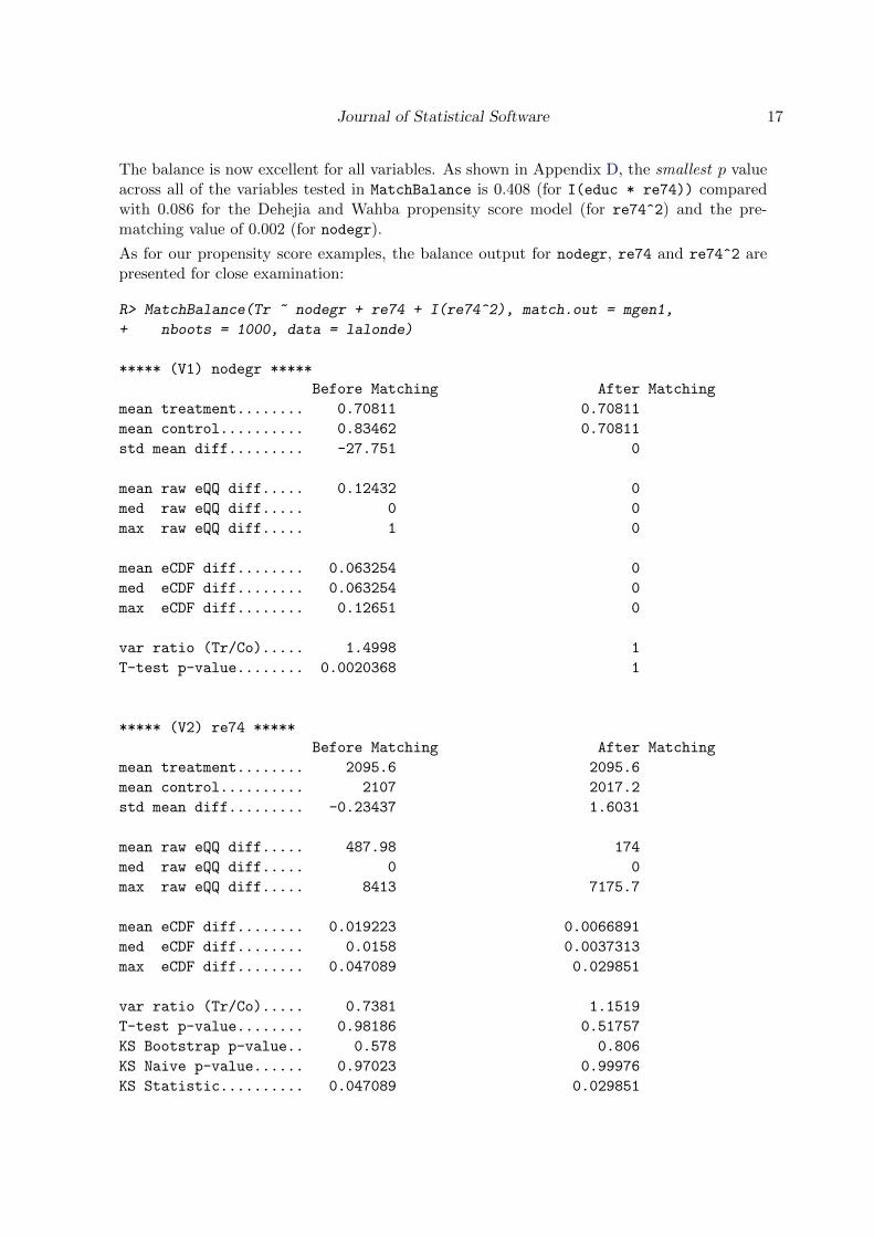
The balance is now excellent for all variables. As shown in Appendix D, the smallest p valueacross all of the variables tested in MatchBalance is 0.408 (for I(educ * re74)) comparedwith 0.086 for the Dehejia and Wahba propensity score model (for re74^2) and the pre-matching value of 0.002 (for nodegr).
As for our propensity score examples, the balance output for nodegr, re74 and re74^2 arepresented for close examination:
R> MatchBalance(Tr ~ nodegr + re74 + I(re74^2), match.out = mgen1,
+ nboots = 1000, data = lalonde)
***** (V1) nodegr *****
Before Matching After Matching
mean treatment........ 0.70811 0.70811
mean control.......... 0.83462 0.70811
std mean diff......... -27.751 0
mean raw eQQ diff..... 0.12432 0
med raw eQQ diff..... 0 0
max raw eQQ diff..... 1 0
mean eCDF diff........ 0.063254 0
med eCDF diff........ 0.063254 0
max eCDF diff........ 0.12651 0
var ratio (Tr/Co)..... 1.4998 1
T-test p-value........ 0.0020368 1
***** (V2) re74 *****
Before Matching After Matching
mean treatment........ 2095.6 2095.6
mean control.......... 2107 2017.2
std mean diff......... -0.23437 1.6031
mean raw eQQ diff..... 487.98 174
med raw eQQ diff..... 0 0
max raw eQQ diff..... 8413 7175.7
mean eCDF diff........ 0.019223 0.0066891
med eCDF diff........ 0.0158 0.0037313
max eCDF diff........ 0.047089 0.029851
var ratio (Tr/Co)..... 0.7381 1.1519
T-test p-value........ 0.98186 0.51757
KS Bootstrap p-value.. 0.578 0.806
KS Naive p-value...... 0.97023 0.99976
KS Statistic.......... 0.047089 0.029851
18 Matching: Multivariate Matching with Automated Balance Optimization in R
***** (V3) I(re74^2) *****
Before Matching After Matching
mean treatment........ 28141434 28141434
mean control.......... 36667413 24686484
std mean diff......... -7.4721 3.0279
mean raw eQQ diff..... 13311731 4823772
med raw eQQ diff..... 0 0
max raw eQQ diff..... 365146387 451383821
mean eCDF diff........ 0.019223 0.0066891
med eCDF diff........ 0.0158 0.0037313
max eCDF diff........ 0.047089 0.029851
var ratio (Tr/Co)..... 0.50382 1.5233
T-test p-value........ 0.51322 0.4652
KS Bootstrap p-value.. 0.578 0.806
KS Naive p-value...... 0.97023 0.99976
KS Statistic.......... 0.047089 0.029851
Before Matching Minimum p.value: 0.0020368
Variable Name(s): nodegr Number(s): 1
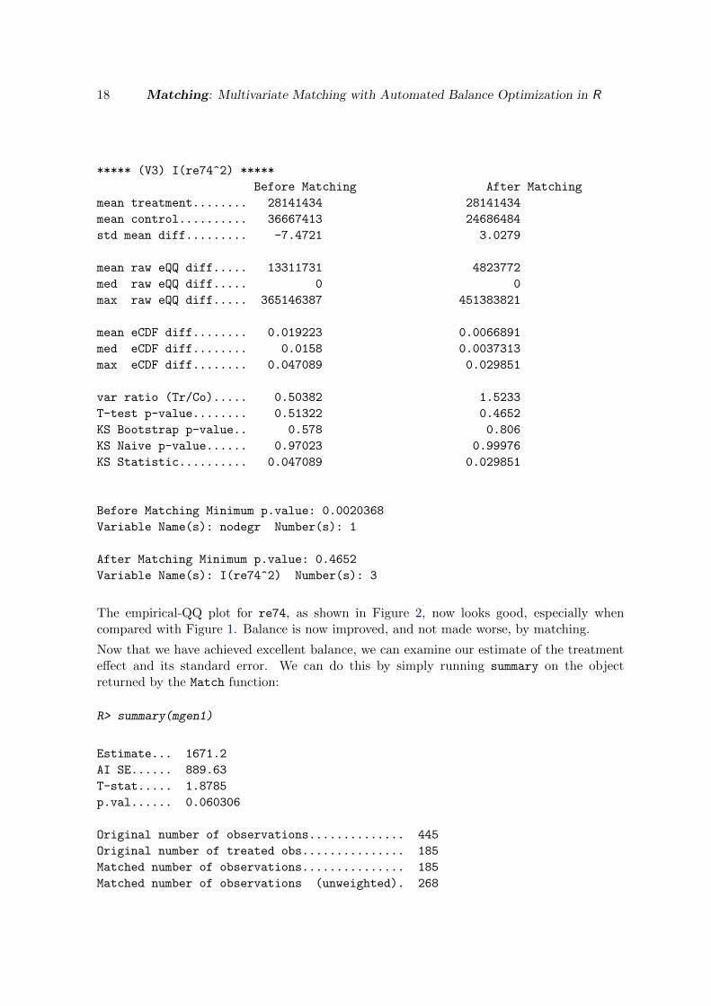
After Matching Minimum p.value: 0.4652
Variable Name(s): I(re74^2) Number(s): 3
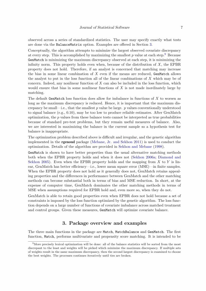
The empirical-QQ plot for re74, as shown in Figure 2, now looks good, especially whencompared with Figure 1. Balance is now improved, and not made worse, by matching.
Now that we have achieved excellent balance, we can examine our estimate of the treatmenteffect and its standard error. We can do this by simply running summary on the objectreturned by the Match function:
R> summary(mgen1)
Estimate... 1671.2
AI SE...... 889.63
T-stat..... 1.8785
p.val...... 0.060306
Original number of observations.............. 445
Original number of treated obs............... 185
Matched number of observations............... 185
Matched number of observations (unweighted). 268

Journal of Statistical Software 19
●●●●●●●●●●●●●●●●●●●●●●●●●●●●●●●●●●●●●●●●●●●●●●●●●●●●●●●●●●●●●●●●●●●●●●●●●●●●●●●●●●●●●●●●●●●●●●●●●●●●●●●●●●●●●●●●●●●●●●●●●●●●●●●●●●●●●●●●●●●●●●●●●●●●●●●●●●●●●●●●●●●●●●●●●●●●●●●●●●●●●●●●●●●●●●●●●●●●●●●●●●●●●●●●●●●●●●●●●●●●●
●●●●●● ●●●●
●●
●●●●● ●
●●●●
●●●● ●
●●●●●
●
●●●●●
●●●● ●
●
●
●
●
0 5000 10000 15000 20000 25000 30000 35000
050
0010
000
1500
020
000
2500
030
000
3500
0
Control Observations
Trea
tmen
t Obs
erva
tions
Figure 2: Empirical-QQ plot of re74 using GenMatch.
The estimate of the treatment effect for the treated is $1,671.20 with a standard error of889.63. By default, the Abadie-Imbens (AI) standard error is printed (Abadie and Imbens2006). In order to also obtain the usual Neyman standard error, one may call the summary
function with the full=TRUE option.
The summary function also provides the number of observations in total (445), the number oftreated observations (185), the number of matched pairs that were produced when the ties areproperly weighted (185), and the number of matched pairs without using the weights whichadjust for ties (268).
3.3. Parallel and cluster processing
GenMatch is a computationally intensive algorithm because it constructs matched datasetsfor each trail set of covariate weights. Fortunately, as with most genetic algorithms, thealgorithm easily parallelizes. This functionality has been built directly in the rgenoud packageand be readily accessed by GenMatch. The parallelization can be used for either multipleCPU computers or a cluster of computers, and makes use of R’s snow (simple network ofworkstations) package (Rossini, Tierney, and Li 2007). Simulations to estimate how well theparallel algorithm scales with multiple CPUs are provided below. On a single computer withmultiple CPUs, the proportion of time saved is almost linear in the number of CPUs if thedataset size is large. For a cluster of separate computers, the algorithm is significantly faster

20 Matching: Multivariate Matching with Automated Balance Optimization in R
for every extra node which is added, but the time savings are significantly less than linear.The exact amount of time saved depends on network latency and a host of other factors.
Two GenMatch options control the parallel processing: cluster and balance. The cluster
option can either be an object of the ‘cluster’ class returned by one of the makeCluster
commands in the snow package or a vector of machine names so that GenMatch can setupthe cluster automatically via secure-shell (SSH). If it is the latter, the vector passed to thecluster option should look like the following:
R> c("localhost", "localhost", "musil", "musil", "deckard")
This vector would create a cluster with four nodes: two on the localhost another on ‘deckard’and two on the machine named ‘musil’. Two nodes on a given machine make sense if themachine has two or more chips/cores. GenMatch will setup a SOCK cluster by a call tomakeSOCKcluster. This will require the user to type in her password for each node as thecluster is by default created via SSH. One can add on user names to the machine name ifit differs from the current shell: username@musil. Other cluster types, such as PVM andMPI, which do not require passwords, can be created by directly calling makeCluster, andthen passing the returned cluster object to GenMatch. For example, one can manually setupa cluster with a direct call to makeCluster as follows:
R> library("snow")
R> library("Matching")
R> data("lalonde")
R> attach(lalonde)
R> cl <- makeCluster(c("musil", "quetelet", "quetelet"), type = "SOCK")
R> X <- cbind(age, educ, black, hisp, married, nodegr, u74, u75, re75, re74)
R> genout <- GenMatch(Tr = treat, X = X, cluster = cl)
R> stopCluster(cl)
Note the stopCluster(cl) command which is needed because we setup the cluster outputof GenMatch. So, we much manually shut the connections down.
The second GenMatch option which controls the behavior of parallel processing is the balanceoption. This is a logical flag which controls if load balancing is done across the cluster.Load balancing can result in better cluster utilization; however, increased communicationcan reduce performance. This options is best used if each individual call to Match takesat least several minutes to calculate or if the nodes in the cluster vary significantly in theirperformance.
Designing parallel software applications is difficult. A lot of work and trail-and-error has goneinto writing the C++ functions which GenMatch relies upon to ensure that they are reliableand fast when run either serially or in parallel. Parallel execution is especially tricky becausean algorithm which may be fast in serial mode can cause unexpected bottlenecks when runin parallel (such as a cache-bottleneck when executing SSE3 instructions via BLAS).
We now explore how well GenMatch scales with additional CPUs by using the following bench-mark code:
R> library("Matching")
R> data("lalonde")
Journal of Statistical Software 21
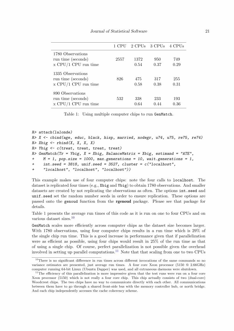
1 CPU 2 CPUs 3 CPUs 4 CPUs
1780 Observationsrun time (seconds) 2557 1372 950 749x CPU/1 CPU run time 0.54 0.37 0.29
1335 Observationsrun time (seconds) 826 475 317 255x CPU/1 CPU run time 0.58 0.38 0.31
890 Observationsrun time (seconds) 532 338 233 193x CPU/1 CPU run time 0.64 0.44 0.36
Table 1: Using multiple computer chips to run GenMatch.
R> attach(lalonde)
R> X <- cbind(age, educ, black, hisp, married, nodegr, u74, u75, re75, re74)
R> Xbig <- rbind(X, X, X, X)
R> Ybig <- c(treat, treat, treat, treat)
R> GenMatch(Tr = Ybig, X = Xbig, BalanceMatrix = Xbig, estimand = "ATE",
+ M = 1, pop.size = 1000, max.generations = 10, wait.generations = 1,
+ int.seed = 3818, unif.seed = 3527, cluster = c("localhost",
+ "localhost", "localhost", "localhost"))
This example makes use of four computer chips: note the four calls to localhost. Thedataset is replicated four times (e.g., Xbig and Ybig) to obtain 1780 observations. And smallerdatasets are created by not replicating the observations as often. The options int.seed andunif.seed set the random number seeds in order to ensure replication. These options arepassed onto the genoud function from the rgenoud package. Please see that package fordetails.
Table 1 presents the average run times of this code as it is run on one to four CPUs and onvarious dataset sizes.10
GenMatch scales more efficiently across computer chips as the dataset size becomes larger.With 1780 observations, using four computer chips results in a run time which is 29% ofthe single chip run time. This is a good increase in performance given that if parallelizationwere as efficient as possible, using four chips would result in 25% of the run time as thatof using a single chip. Of course, perfect parallelization is not possible given the overheadinvolved in setting up parallel computations.11 Note that that scaling from one to two CPUs
10There is no significant difference in run times across different invocations of the same commands so novariance estimates are presented, just average run times. A four core Xeon processor (5150 @ 2.66GHz)computer running 64-bit Linux (Ubuntu Dapper) was used, and all extraneous daemons were shutdown.
11The efficiency of this parallelization is more impressive given that the test runs were run on a four coreXeon processor (5150) which is not really a four core chip. This chip actually consists of two (dual-core)Woodcrest chips. The two chips have no way to communicate directly with each other. All communicationsbetween them have to go through a shared front-side bus with the memory controller hub, or north bridge.And each chip independently accesses the cache coherency scheme.
22 Matching: Multivariate Matching with Automated Balance Optimization in R
is closer to the theoretical efficiency bound (1.08 = 0.54/0.5) then scaling from one to fourchips (1.16 = 0.29/0.25). This may be due to the issue pointed out in Footnote 11.
With 890 observations, using four CPUs takes 36% of the run time as only using one CPU.This is a significantly smaller efficiency gain than that achieved with the dataset with 1780observations.
It is clear from Table 1 that the computational time it takes to execute a matching algorithmdoes not increase linearly with sample size. The computational time increases as a polynomialof the sample size, and the average asymptotic order of the Match function is approximatelyO(N2)log(N).12 The run times in Table 1 are generally consistent with this. Although theMatch function increases in polynomial time, the problem which GenMatch attempts to solve(that of finding the best distance metric) increases exponentially in sample size, just like thetraveling salesman problem. That is, the set of possible matched datasets grows exponentiallywith sample size.
4. Conclusion
The functions in Matching have many more options than can be reviewed in this brief paper.For additional details see the manual pages for the functions included in the R package. TheMatching package includes four functions in addition to Match, GenMatch, and MatchBalance:Matchby (for large datasets), qqstats (descriptive eQQ statistics), ks.boot (bootstrap ver-sion of ks.test) and balanceUV (univariate balance statistics).
A great deal of effort has been made in order to ensure that the matching functions are asfast as possible. The computationally intensive functions are written in C++ which makeextensive use of the BLAS libraries, and GenMatch can be used with multiple computers,CPUs or cores to perform parallel computations. The C++ functions have been written sothat the GNU g++ compiler does a good job of optimizing them. Indeed, compiling theMatching package with the Intel C++ compiler does not result in faster code. This is unusualwith floating point code, and is the result of carefully writing code so that the GNU compileris able to optimize it aggressively. Moreover, the Matchby function has been tuned to workwell with large datasets.
After intensive benchmarking and instrumenting the code, it was determined that performanceon OS X was seriously limited because the default OS X memory allocator is not as efficient asLea (2000)’s malloc given the frequent memory allocations made by the matching code. Thematching algorithm was rewritten in order to be more efficient with memory on all platforms,and on OS X, Matching is compiled against Lea’s malloc which is something more packagesfor R may wish to do. For details see Sekhon (2006b).
The literature on matching methods is developing quickly with new innovations being madeby a variety of researchers in fields ranging from economics, epidemiology and political scienceto sociology and statistics. Hence, new options are being added frequently.
12The precise asymptotic order is difficult to calculate because assumptions have to be made about variousfeatures of the data such as the proportion of ties.
Journal of Statistical Software 23
References
Abadie A (2002). “Bootstrap Tests for Distributional Treatment Effect in Instrumental Vari-able Models.” Journal of the American Statistical Association, 97(457), 284–292.
Abadie A, Imbens G (2006). “Large Sample Properties of Matching Estimators for AverageTreatment Effects.” Econometrica, 74, 235–267.
Andam KS, Ferraro PJ, Pfaff A, Sanchez-Azofeifa GA, Robalino JA (2008). “Measuring theEffectiveness of Protected Area Networks in Reducing Deforestation.” Proceedings of theNational Academy of Sciences, 105(42), 16089–16094.
Barnard J, Frangakis CE, Hill JL, Rubin DB (2003). “Principal Stratification Approach toBroken Randomized Experiments: A Case Study of School Choice Vouchers in New YorkCity.” Journal of the American Statistical Association, 98(462), 299–323.
Bowers J, Hansen B (2005). “Attributing Effects to A Cluster Randomized Get-Out-The-Vote Campaign.” Technical Report 448, Statistics Department, Uni-versity of Michigan. URL http://www-personal.umich.edu/~jwbowers/PAPERS/
bowershansen2006-10TechReport.pdf.
Christakis NA, Iwashyna TI (2003). “The Health Impact of Health Care on Families: Amatched cohort study of hospice use by decedents and mortality outcomes in surviving,widowed spouses.” Social Science & Medicine, 57(3), 465–475.
Cochran WG, Rubin DB (1973). “Controlling Bias in Observational Studies: A Review.”Sankhya A, 35, 417–446.
Dawid AP (1979). “Conditional Independence in Statistical Theory.” Journal of the RoyalStatistical Society B, 41(1), 1–31.
Dehejia R, Wahba S (1999). “Causal Effects in Non-Experimental Studies: Re-Evaluatingthe Evaluation of Training Programs.” Journal of the American Statistical Association,94(448), 1053–1062.
Dehejia RH, Wahba S (2002). “Propensity Score Matching Methods for NonexperimentalCausal Studies.” Review of Economics and Statistics, 84(1), 151–161.
Diamond A, Sekhon JS (2005). “Genetic Matching for Estimating Causal Effects: A GeneralMultivariate Matching Method for Achieving Balance in Observational Studies.” Technicalreport, Department of Political Science, UC Berkeley. URL http://sekhon.berkeley.
edu/papers/GenMatch.pdf.
Diprete TA, Engelhardt H (2004). “Estimating Causal Effects with Matching Methods inthe Presence and Absence of Bias Cancellation.” Sociological Methods & Research, 32(4),501–528.
Eggers A, Hainmueller J (2009). “The Value of Political Power: Estimating Returns to Officein Post-War British Politics.” American Political Science Review, 103(4), 513–533.
24 Matching: Multivariate Matching with Automated Balance Optimization in R
Fechner GT (1966). Elements of Psychophysics, Volume 1. Rinehart & Winston, New York.Translated by Helmut E. Adler and edited by D. H. Howes and E. G. Boring.
Gilligan MJ, Sergenti EJ (2008). “Do UN Interventions Cause Peace? Using Matching toImprove Causal Inference.” Quarterly Journal of Political Science, 3, 89–122.
Gordon SC (2009). “Assessing Partisan Bias in Federal Public Corruption Prosecutions.”American Political Science Review, 103(4), 534–554.
Hansen BB (2004). “Full Matching in an Observational Study of Coaching for the SAT.”Journal of the American Statistical Association, 99, 609–618.
Hansen BB, Klopfer SO (2006). “Optimal Full Matching and Related Designs via NetworkFlows.” Journal of Computational and Graphical Statistics, 15, 609–627.
Heckman JJ, Ichimura H, Smith J, Todd P (1998). “Characterizing Selection Bias UsingExperimental Data.” Econometrica, 66(5), 1017–1098.
Heinrich CJ (2007). “Demand and Supply-Side Determinants of Conditional Cash TransferProgram Effectiveness.” World Development, 35(1), 121–143.
Herron M, Wand J (2007). “Assessing Partisan Bias in Voting Technology: The Case of the2004 New Hampshire Recount.” Electoral Studies, 26(2), 247–261.
Holland PW (1986). “Statistics and Causal Inference.” Journal of the American StatisticalAssociation, 81(396), 945–960.
Hopkins DJ (2010). “Politicized Places: Explaining Where and When Immigrants ProvokeLocal Opposition.” American Political Science Review, 104(1), 40–60.
Horvitz DG, Thompson DJ (1952). “A Generalization of Sampling without Replacement froma Finite Universe.” Journal of the American Statistical Association, 47, 663–685.
Imai K (2005). “Do Get-Out-The-Vote Calls Reduce Turnout? The Importance of StatisticalMethods for Field Experiments.” American Political Science Review, 99(2), 283–300.
LaLonde R (1986). “Evaluating the Econometric Evaluations of Training Programs withExperimental Data.” American Economic Review, 76, 604–20.
Lea D (2000). “A Memory Allocator.” URL http://gee.cs.oswego.edu/dl/html/malloc.
html.
Lenz GS, Ladd JM (2009). “Exploiting a Rare Communication Shift to Document the Per-suasive Power of the News Media.” American Journal of Political Science, 53(2), 394–410.
Mebane, Jr WR, Sekhon JS (2011). “Genetic Optimization Using Derivatives: The rgenoudPackage for R.” Journal of Statistical Software, 42(11), 1–26. URL http://www.jstatsoft.
org/v42/i11/.
Morgan SL, Harding DJ (2006). “Matching Estimators of Causal Effects: Prospects andPitfalls in Theory and Practice.” Sociological Methods & Research, 35(1), 3–60.
Journal of Statistical Software 25
Nix AE, Vose MD (1992). “Modeling Genetic Algorithms with Markov Chains.” Annals ofMathematics and Artificial Intelligence, 5, 79–88.
Raessler S, Rubin D (2005). “Complications When Using Nonrandomized Job Training Datato Draw Causal Inferences.” In Proceedings of the International Statistical Institute. URLhttp://www.websm.org/uploadi/editor/1132827726ISI.Susie.doc.
R Development Core Team (2011). R: A Language and Environment for Statistical Computing.R Foundation for Statistical Computing, Vienna, Austria. ISBN 3-900051-07-0, URL http:
//www.R-project.org/.
Rosenbaum PR (1989). “Optimal Matching for Observational Studies.” Journal of the Amer-ican Statistical Association, 84(408), 1024–1032.
Rosenbaum PR (1991). “A Characterization of Optimal Designs for Observational Studies.”Journal of the Royal Statistical Society B, 53(3), 597–610.
Rosenbaum PR (2002). Observational Studies. 2nd edition. Springer-Verlag, New York.
Rosenbaum PR, Rubin DB (1983). “The Central Role of the Propensity Score in ObservationalStudies for Causal Effects.” Biometrika, 70(1), 41–55.
Rosenbaum PR, Rubin DB (1985). “Constructing a Control Group Using MultivariateMatched Sampling Methods That Incorporate the Propensity Score.” The American Statis-tician, 39(1), 33–38.
Rossini AJ, Tierney L, Li N (2007). “Simple Parallel Statistical Computing in R.” Journal ofComputational and Graphical Statistics, 16(2), 399–420.
Rubin D, Stuart EA (2006). “Affinely Invariant Matching Methods with Discriminant Mix-tures of Proportional Ellipsoidally Symmetric Distributions.” The Annals of Statistics,34(4), 1814–1826.
Rubin DB (1974). “Estimating Causal Effects of Treatments in Randomized and Nonrandom-ized Studies.” Journal of Educational Psychology, 66, 688–701.
Rubin DB (1976a). “Multivariate Matching Methods That are Equal Percent Bias Reducing,I: Some Examples.” Biometrics, 32(1), 109–120.
Rubin DB (1976b). “Multivariate Matching Methods That are Equal Percent Bias Reducing,II: Maximums on Bias Reduction for Fixed Sample Sizes.” Biometrics, 32(1), 121–132.
Rubin DB (1977). “Assignment to a Treatment Group on the Basis of a Covariate.” Journalof Educational Statistics, 2, 1–26.
Rubin DB (1978). “Bayesian Inference for Causal Effects: The Role of Randomization.” TheAnnals of Statistics, 6(1), 34–58.
Rubin DB (1979). “Using Multivariate Sampling and Regression Adjustment to Control Biasin Observational Studies.” Journal of the American Statistical Association, 74, 318–328.
Rubin DB (1980). “Bias Reduction Using Mahalanobis-Metric Matching.” Biometrics, 36(2),293–298.
26 Matching: Multivariate Matching with Automated Balance Optimization in R
Rubin DB (1990). “Comment: Neyman (1923) and Causal Inference in Experiments andObservational Studies.” Statistical Science, 5(4), 472–480.
Rubin DB (1997). “Estimating Causal Effects from Large Data Sets Using Propensity Scores.”Annals of Internal Medicine, 127(8S), 757–763.
Rubin DB (2001). “Using Propensity Scores to Help Design Observational Studies: Applica-tion to the Tobacco Litigation.” Health Services & Outcomes Research Methodology, 2(1),169–188.
Rubin DB (2006). Matched Sampling for Causal Effects. Cambridge University Press, NewYork.
Rubin DB, Thomas N (1992). “Affinely Invariant Matching Methods with Ellipsoidal Distri-butions.” The Annals of Statistics, 20(2), 1079–1093.
Sekhon JS (2006a). “Alternative Balance Metrics for Bias Reduction in Matching Methodsfor Causal Inference.” Technical report, Department of Political Science, UC Berkeley. URLhttp://sekhon.berkeley.edu/papers/SekhonBalanceMetrics.pdf.
Sekhon JS (2006b). “The Art of Benchmarking: Evaluating the Performance of R on Linuxand OS X.” The Political Methodologist, 14(1).
Sekhon JS, Grieve R (2011). “A Non-Parametric Matching Method for Bias Adjustment withApplications to Economic Evaluations.” Health Economics. Forthcoming.
Sekhon JS, Mebane Jr WR (1998). “Genetic Optimization Using Derivatives: Theory andApplication to Nonlinear Models.” Political Analysis, 7, 189–203.
Smith HL (1997). “Matching with Multiple Controls to Estimate Treatment Effects in Ob-servational Studies.” Sociological Methodology, 27, 305–353.
Splawa-Neyman J (1923). “On the Application of Probability Theory to Agricultural Exper-iments. Essay on Principles. Section 9.” Statistical Science, 5(4), 465–472. Trans. DorotaM. Dabrowska and Terence P. Speed.
Vose MD (1993). “Modeling Simple Genetic Algorithms.” In LD Whitley (ed.), Foundationsof Genetic Algorithms 2. Morgan Kaufmann, San Mateo, CA.
Winship C, Morgan S (1999). “The Estimation of Causal Effects from Observational Data.”Annual Review of Sociology, 25, 659–707.
Journal of Statistical Software 27
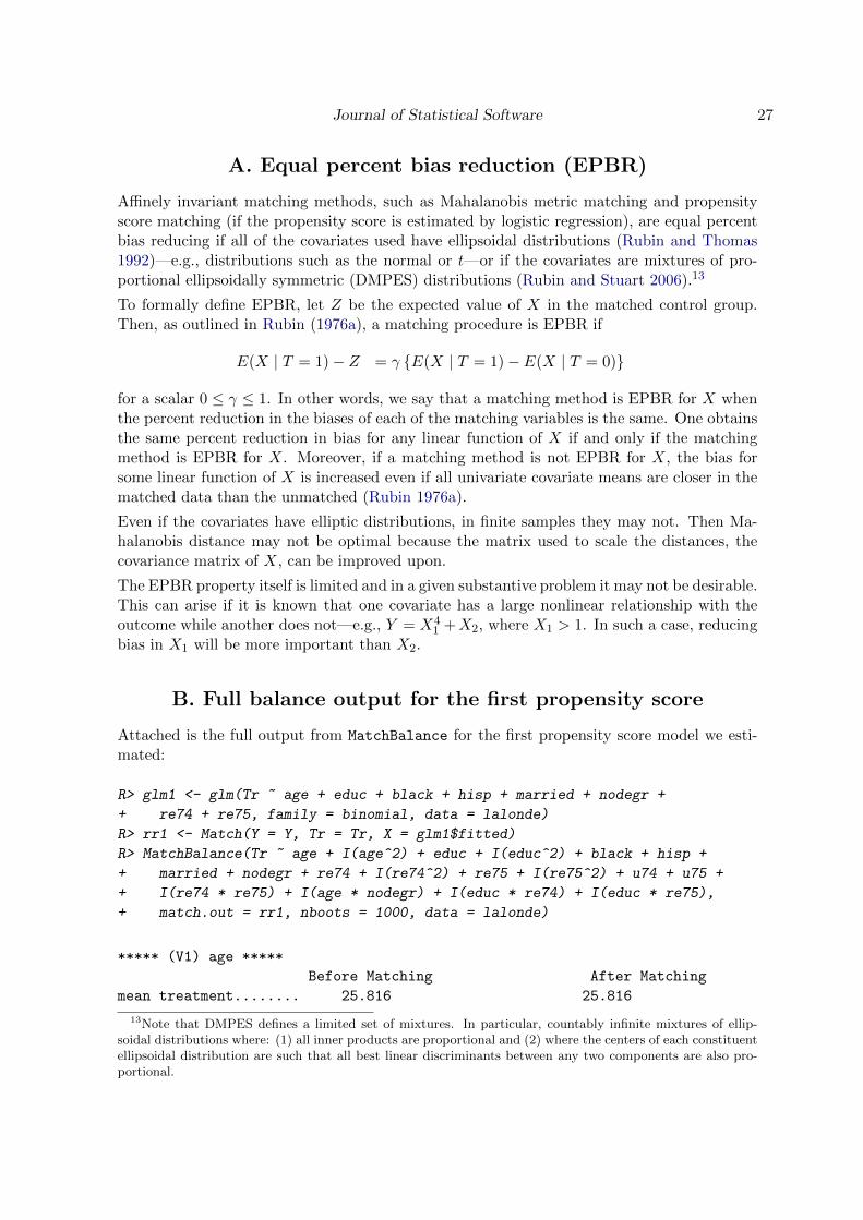
A. Equal percent bias reduction (EPBR)
Affinely invariant matching methods, such as Mahalanobis metric matching and propensityscore matching (if the propensity score is estimated by logistic regression), are equal percentbias reducing if all of the covariates used have ellipsoidal distributions (Rubin and Thomas1992)—e.g., distributions such as the normal or t—or if the covariates are mixtures of pro-portional ellipsoidally symmetric (DMPES) distributions (Rubin and Stuart 2006).13
To formally define EPBR, let Z be the expected value of X in the matched control group.Then, as outlined in Rubin (1976a), a matching procedure is EPBR if
E(X | T = 1)− Z = γ {E(X | T = 1)− E(X | T = 0)}
for a scalar 0 ≤ γ ≤ 1. In other words, we say that a matching method is EPBR for X whenthe percent reduction in the biases of each of the matching variables is the same. One obtainsthe same percent reduction in bias for any linear function of X if and only if the matchingmethod is EPBR for X. Moreover, if a matching method is not EPBR for X, the bias forsome linear function of X is increased even if all univariate covariate means are closer in thematched data than the unmatched (Rubin 1976a).
Even if the covariates have elliptic distributions, in finite samples they may not. Then Ma-halanobis distance may not be optimal because the matrix used to scale the distances, thecovariance matrix of X, can be improved upon.
The EPBR property itself is limited and in a given substantive problem it may not be desirable.This can arise if it is known that one covariate has a large nonlinear relationship with theoutcome while another does not—e.g., Y = X4
1 +X2, where X1 > 1. In such a case, reducingbias in X1 will be more important than X2.
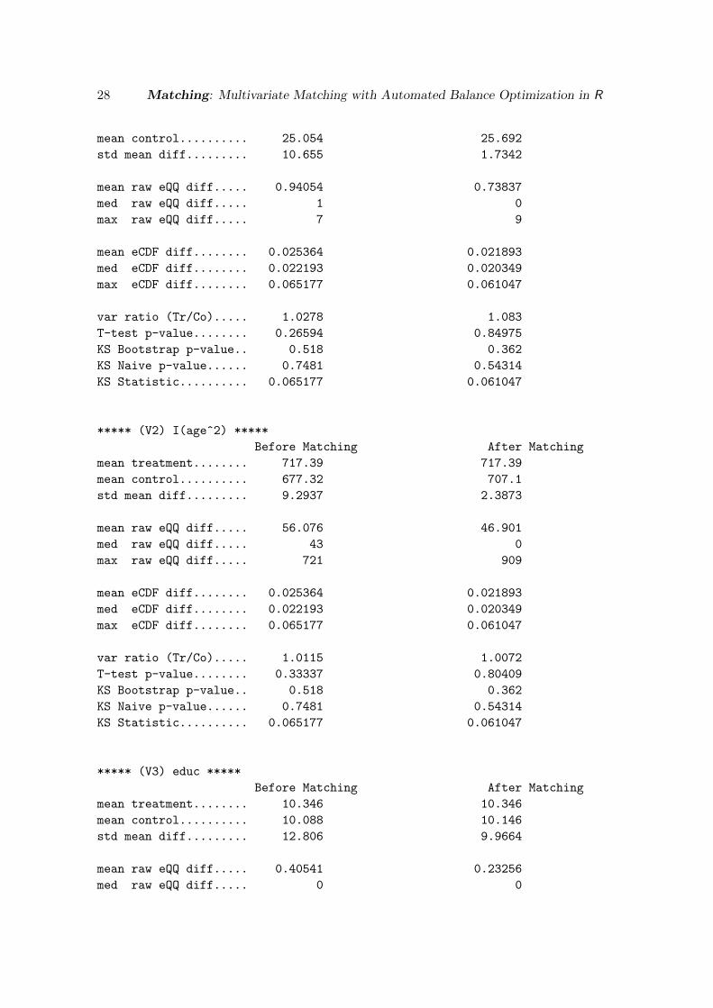
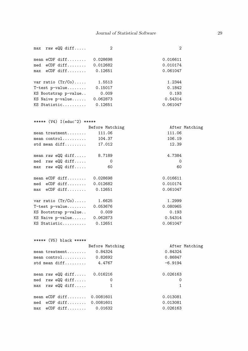
B. Full balance output for the first propensity score
Attached is the full output from MatchBalance for the first propensity score model we esti-mated:
R> glm1 <- glm(Tr ~ age + educ + black + hisp + married + nodegr +
+ re74 + re75, family = binomial, data = lalonde)
R> rr1 <- Match(Y = Y, Tr = Tr, X = glm1$fitted)
R> MatchBalance(Tr ~ age + I(age^2) + educ + I(educ^2) + black + hisp +
+ married + nodegr + re74 + I(re74^2) + re75 + I(re75^2) + u74 + u75 +
+ I(re74 * re75) + I(age * nodegr) + I(educ * re74) + I(educ * re75),
+ match.out = rr1, nboots = 1000, data = lalonde)
***** (V1) age *****
Before Matching After Matching
mean treatment........ 25.816 25.816
13Note that DMPES defines a limited set of mixtures. In particular, countably infinite mixtures of ellip-soidal distributions where: (1) all inner products are proportional and (2) where the centers of each constituentellipsoidal distribution are such that all best linear discriminants between any two components are also pro-portional.
28 Matching: Multivariate Matching with Automated Balance Optimization in R
mean control.......... 25.054 25.692
std mean diff......... 10.655 1.7342
mean raw eQQ diff..... 0.94054 0.73837
med raw eQQ diff..... 1 0
max raw eQQ diff..... 7 9
mean eCDF diff........ 0.025364 0.021893
med eCDF diff........ 0.022193 0.020349
max eCDF diff........ 0.065177 0.061047
var ratio (Tr/Co)..... 1.0278 1.083
T-test p-value........ 0.26594 0.84975
KS Bootstrap p-value.. 0.518 0.362
KS Naive p-value...... 0.7481 0.54314
KS Statistic.......... 0.065177 0.061047
***** (V2) I(age^2) *****
Before Matching After Matching
mean treatment........ 717.39 717.39
mean control.......... 677.32 707.1
std mean diff......... 9.2937 2.3873
mean raw eQQ diff..... 56.076 46.901
med raw eQQ diff..... 43 0
max raw eQQ diff..... 721 909
mean eCDF diff........ 0.025364 0.021893
med eCDF diff........ 0.022193 0.020349
max eCDF diff........ 0.065177 0.061047
var ratio (Tr/Co)..... 1.0115 1.0072
T-test p-value........ 0.33337 0.80409
KS Bootstrap p-value.. 0.518 0.362
KS Naive p-value...... 0.7481 0.54314
KS Statistic.......... 0.065177 0.061047
***** (V3) educ *****
Before Matching After Matching
mean treatment........ 10.346 10.346
mean control.......... 10.088 10.146
std mean diff......... 12.806 9.9664
mean raw eQQ diff..... 0.40541 0.23256
med raw eQQ diff..... 0 0
Journal of Statistical Software 29
max raw eQQ diff..... 2 2
mean eCDF diff........ 0.028698 0.016611
med eCDF diff........ 0.012682 0.010174
max eCDF diff........ 0.12651 0.061047
var ratio (Tr/Co)..... 1.5513 1.2344
T-test p-value........ 0.15017 0.1842
KS Bootstrap p-value.. 0.009 0.193
KS Naive p-value...... 0.062873 0.54314
KS Statistic.......... 0.12651 0.061047
***** (V4) I(educ^2) *****
Before Matching After Matching
mean treatment........ 111.06 111.06
mean control.......... 104.37 106.19
std mean diff......... 17.012 12.39
mean raw eQQ diff..... 8.7189 4.7384
med raw eQQ diff..... 0 0
max raw eQQ diff..... 60 60
mean eCDF diff........ 0.028698 0.016611
med eCDF diff........ 0.012682 0.010174
max eCDF diff........ 0.12651 0.061047
var ratio (Tr/Co)..... 1.6625 1.2999
T-test p-value........ 0.053676 0.080965
KS Bootstrap p-value.. 0.009 0.193
KS Naive p-value...... 0.062873 0.54314
KS Statistic.......... 0.12651 0.061047
***** (V5) black *****
Before Matching After Matching
mean treatment........ 0.84324 0.84324
mean control.......... 0.82692 0.86847
std mean diff......... 4.4767 -6.9194
mean raw eQQ diff..... 0.016216 0.026163
med raw eQQ diff..... 0 0
max raw eQQ diff..... 1 1
mean eCDF diff........ 0.0081601 0.013081
med eCDF diff........ 0.0081601 0.013081
max eCDF diff........ 0.01632 0.026163
30 Matching: Multivariate Matching with Automated Balance Optimization in R
var ratio (Tr/Co)..... 0.92503 1.1572
T-test p-value........ 0.64736 0.40214
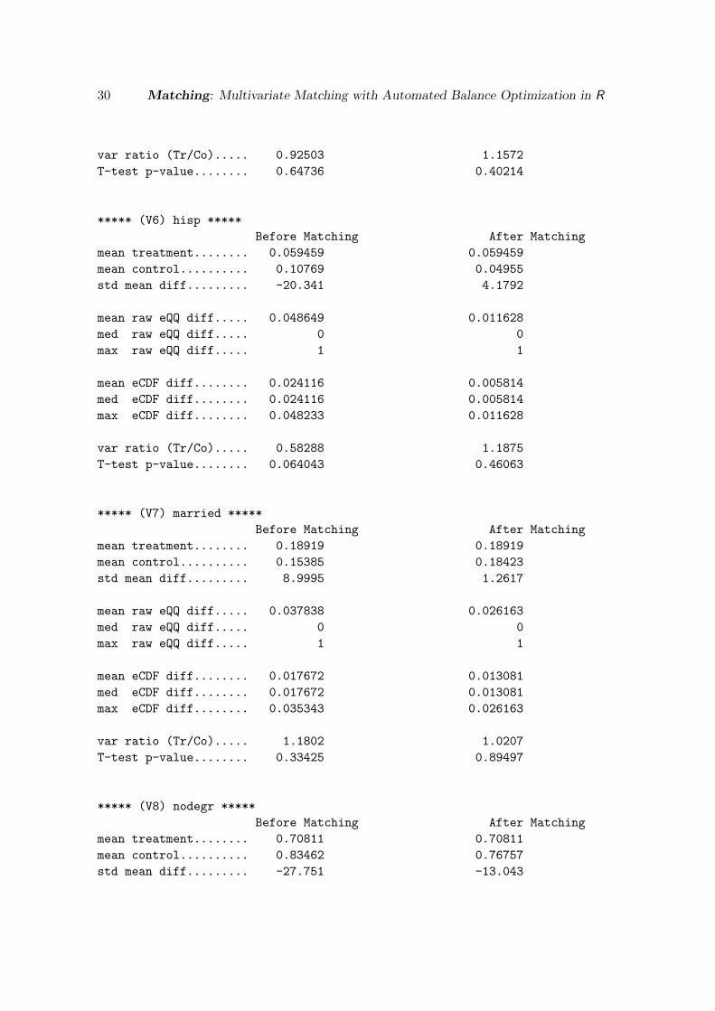
***** (V6) hisp *****
Before Matching After Matching
mean treatment........ 0.059459 0.059459
mean control.......... 0.10769 0.04955
std mean diff......... -20.341 4.1792
mean raw eQQ diff..... 0.048649 0.011628
med raw eQQ diff..... 0 0
max raw eQQ diff..... 1 1
mean eCDF diff........ 0.024116 0.005814
med eCDF diff........ 0.024116 0.005814
max eCDF diff........ 0.048233 0.011628
var ratio (Tr/Co)..... 0.58288 1.1875
T-test p-value........ 0.064043 0.46063
***** (V7) married *****
Before Matching After Matching
mean treatment........ 0.18919 0.18919
mean control.......... 0.15385 0.18423
std mean diff......... 8.9995 1.2617
mean raw eQQ diff..... 0.037838 0.026163
med raw eQQ diff..... 0 0
max raw eQQ diff..... 1 1
mean eCDF diff........ 0.017672 0.013081
med eCDF diff........ 0.017672 0.013081
max eCDF diff........ 0.035343 0.026163
var ratio (Tr/Co)..... 1.1802 1.0207
T-test p-value........ 0.33425 0.89497
***** (V8) nodegr *****
Before Matching After Matching
mean treatment........ 0.70811 0.70811
mean control.......... 0.83462 0.76757
std mean diff......... -27.751 -13.043

Journal of Statistical Software 31
mean raw eQQ diff..... 0.12432 0.043605
med raw eQQ diff..... 0 0
max raw eQQ diff..... 1 1
mean eCDF diff........ 0.063254 0.021802
med eCDF diff........ 0.063254 0.021802
max eCDF diff........ 0.12651 0.043605
var ratio (Tr/Co)..... 1.4998 1.1585
T-test p-value........ 0.0020368 0.0071385
***** (V9) re74 *****
Before Matching After Matching
mean treatment........ 2095.6 2095.6
mean control.......... 2107 2193.3
std mean diff......... -0.23437 -2.0004
mean raw eQQ diff..... 487.98 869.16
med raw eQQ diff..... 0 0
max raw eQQ diff..... 8413 10305
mean eCDF diff........ 0.019223 0.054701
med eCDF diff........ 0.0158 0.050872
max eCDF diff........ 0.047089 0.12209
var ratio (Tr/Co)..... 0.7381 0.75054
T-test p-value........ 0.98186 0.84996
KS Bootstrap p-value.. 0.594 0.001
KS Naive p-value...... 0.97023 0.011858
KS Statistic.......... 0.047089 0.12209
***** (V10) I(re74^2) *****
Before Matching After Matching
mean treatment........ 28141434 28141434
mean control.......... 36667413 36454686
std mean diff......... -7.4721 -7.2857
mean raw eQQ diff..... 13311731 14189969
med raw eQQ diff..... 0 0
max raw eQQ diff..... 365146387 566243911
mean eCDF diff........ 0.019223 0.054701
med eCDF diff........ 0.0158 0.050872
max eCDF diff........ 0.047089 0.12209
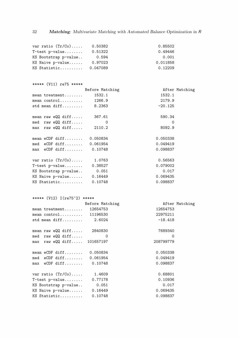
32 Matching: Multivariate Matching with Automated Balance Optimization in R
var ratio (Tr/Co)..... 0.50382 0.85502
T-test p-value........ 0.51322 0.49446
KS Bootstrap p-value.. 0.594 0.001
KS Naive p-value...... 0.97023 0.011858
KS Statistic.......... 0.047089 0.12209
***** (V11) re75 *****
Before Matching After Matching
mean treatment........ 1532.1 1532.1
mean control.......... 1266.9 2179.9
std mean diff......... 8.2363 -20.125
mean raw eQQ diff..... 367.61 590.34
med raw eQQ diff..... 0 0
max raw eQQ diff..... 2110.2 8092.9
mean eCDF diff........ 0.050834 0.050338
med eCDF diff........ 0.061954 0.049419
max eCDF diff........ 0.10748 0.098837
var ratio (Tr/Co)..... 1.0763 0.56563
T-test p-value........ 0.38527 0.079002
KS Bootstrap p-value.. 0.051 0.017
KS Naive p-value...... 0.16449 0.069435
KS Statistic.......... 0.10748 0.098837
***** (V12) I(re75^2) *****
Before Matching After Matching
mean treatment........ 12654753 12654753
mean control.......... 11196530 22975211
std mean diff......... 2.6024 -18.418
mean raw eQQ diff..... 2840830 7689340
med raw eQQ diff..... 0 0
max raw eQQ diff..... 101657197 208799779
mean eCDF diff........ 0.050834 0.050338
med eCDF diff........ 0.061954 0.049419
max eCDF diff........ 0.10748 0.098837
var ratio (Tr/Co)..... 1.4609 0.68801
T-test p-value........ 0.77178 0.10936
KS Bootstrap p-value.. 0.051 0.017
KS Naive p-value...... 0.16449 0.069435
KS Statistic.......... 0.10748 0.098837
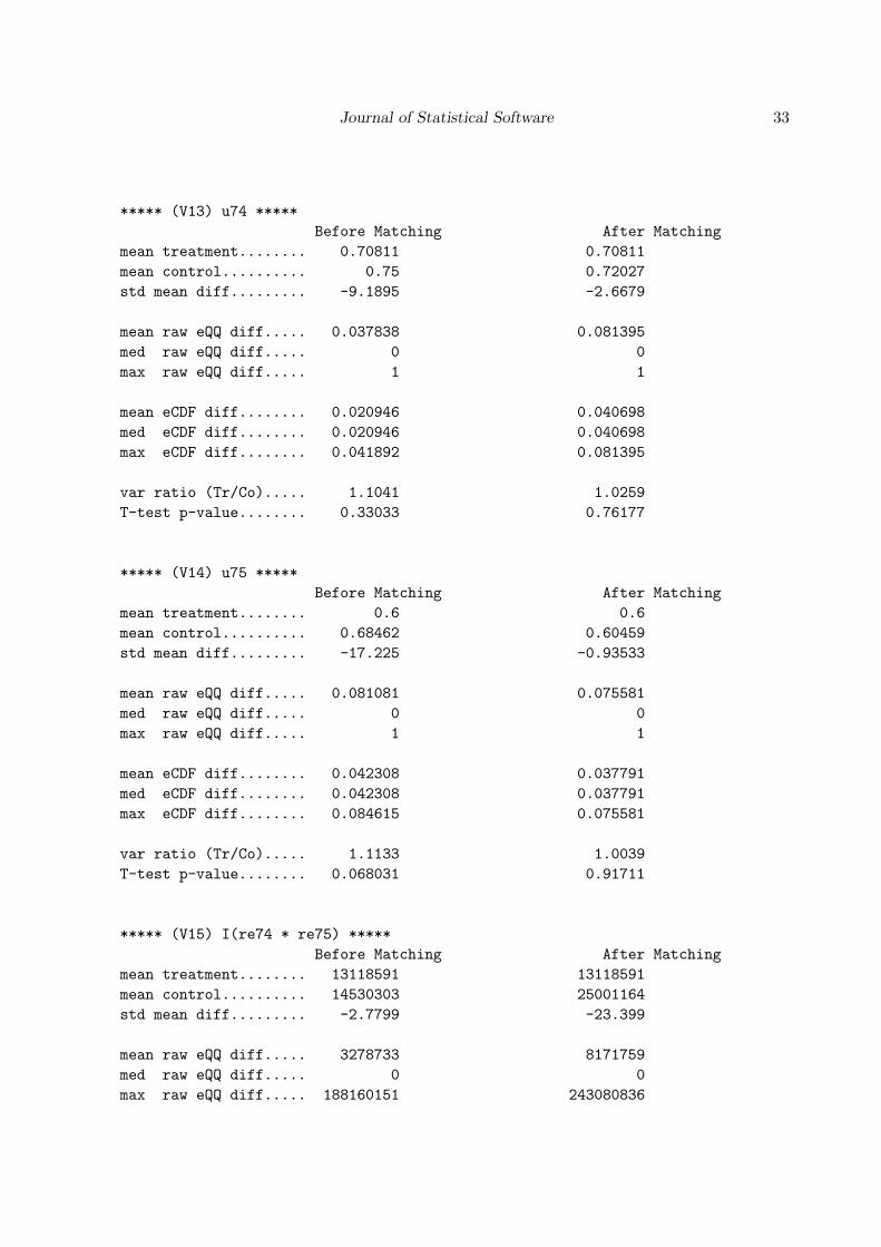
Journal of Statistical Software 33
***** (V13) u74 *****
Before Matching After Matching
mean treatment........ 0.70811 0.70811
mean control.......... 0.75 0.72027
std mean diff......... -9.1895 -2.6679
mean raw eQQ diff..... 0.037838 0.081395
med raw eQQ diff..... 0 0
max raw eQQ diff..... 1 1
mean eCDF diff........ 0.020946 0.040698
med eCDF diff........ 0.020946 0.040698
max eCDF diff........ 0.041892 0.081395
var ratio (Tr/Co)..... 1.1041 1.0259
T-test p-value........ 0.33033 0.76177
***** (V14) u75 *****
Before Matching After Matching
mean treatment........ 0.6 0.6
mean control.......... 0.68462 0.60459
std mean diff......... -17.225 -0.93533
mean raw eQQ diff..... 0.081081 0.075581
med raw eQQ diff..... 0 0
max raw eQQ diff..... 1 1
mean eCDF diff........ 0.042308 0.037791
med eCDF diff........ 0.042308 0.037791
max eCDF diff........ 0.084615 0.075581
var ratio (Tr/Co)..... 1.1133 1.0039
T-test p-value........ 0.068031 0.91711
***** (V15) I(re74 * re75) *****
Before Matching After Matching
mean treatment........ 13118591 13118591
mean control.......... 14530303 25001164
std mean diff......... -2.7799 -23.399
mean raw eQQ diff..... 3278733 8171759
med raw eQQ diff..... 0 0
max raw eQQ diff..... 188160151 243080836

34 Matching: Multivariate Matching with Automated Balance Optimization in R
mean eCDF diff........ 0.022723 0.04676
med eCDF diff........ 0.014449 0.046512
max eCDF diff........ 0.061019 0.09593
var ratio (Tr/Co)..... 0.69439 0.33337
T-test p-value........ 0.79058 0.11452
KS Bootstrap p-value.. 0.324 0.005
KS Naive p-value...... 0.81575 0.084363
KS Statistic.......... 0.061019 0.09593
***** (V16) I(age * nodegr) *****
Before Matching After Matching
mean treatment........ 17.968 17.968
mean control.......... 20.608 19.591
std mean diff......... -20.144 -12.388
mean raw eQQ diff..... 2.7189 1.3866
med raw eQQ diff..... 1 0
max raw eQQ diff..... 18 17
mean eCDF diff........ 0.020386 0.019732
med eCDF diff........ 0.0061331 0.011628
max eCDF diff........ 0.12651 0.072674
var ratio (Tr/Co)..... 1.3301 1.0752
T-test p-value........ 0.027633 0.069335
KS Bootstrap p-value.. 0.031 0.195
KS Naive p-value...... 0.062873 0.32369
KS Statistic.......... 0.12651 0.072674
***** (V17) I(educ * re74) *****
Before Matching After Matching
mean treatment........ 22899 22899
mean control.......... 21067 21812
std mean diff......... 3.191 1.8935
mean raw eQQ diff..... 4775.1 9105.7
med raw eQQ diff..... 0 0
max raw eQQ diff..... 173996 233352
mean eCDF diff........ 0.018141 0.057045
med eCDF diff........ 0.015281 0.049419
max eCDF diff........ 0.04553 0.11919
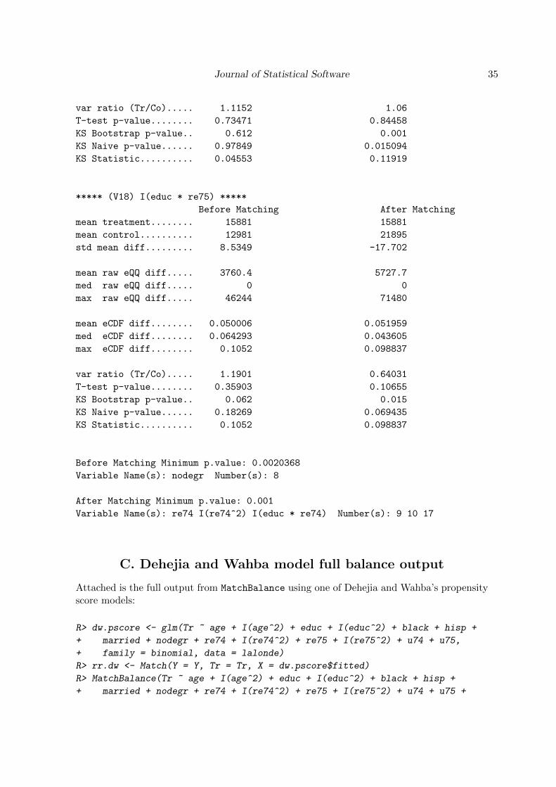
Journal of Statistical Software 35
var ratio (Tr/Co)..... 1.1152 1.06
T-test p-value........ 0.73471 0.84458
KS Bootstrap p-value.. 0.612 0.001
KS Naive p-value...... 0.97849 0.015094
KS Statistic.......... 0.04553 0.11919
***** (V18) I(educ * re75) *****
Before Matching After Matching
mean treatment........ 15881 15881
mean control.......... 12981 21895
std mean diff......... 8.5349 -17.702
mean raw eQQ diff..... 3760.4 5727.7
med raw eQQ diff..... 0 0
max raw eQQ diff..... 46244 71480
mean eCDF diff........ 0.050006 0.051959
med eCDF diff........ 0.064293 0.043605
max eCDF diff........ 0.1052 0.098837
var ratio (Tr/Co)..... 1.1901 0.64031
T-test p-value........ 0.35903 0.10655
KS Bootstrap p-value.. 0.062 0.015
KS Naive p-value...... 0.18269 0.069435
KS Statistic.......... 0.1052 0.098837
Before Matching Minimum p.value: 0.0020368
Variable Name(s): nodegr Number(s): 8
After Matching Minimum p.value: 0.001
Variable Name(s): re74 I(re74^2) I(educ * re74) Number(s): 9 10 17
C. Dehejia and Wahba model full balance output
Attached is the full output from MatchBalance using one of Dehejia and Wahba’s propensityscore models:
R> dw.pscore <- glm(Tr ~ age + I(age^2) + educ + I(educ^2) + black + hisp +
+ married + nodegr + re74 + I(re74^2) + re75 + I(re75^2) + u74 + u75,
+ family = binomial, data = lalonde)
R> rr.dw <- Match(Y = Y, Tr = Tr, X = dw.pscore$fitted)
R> MatchBalance(Tr ~ age + I(age^2) + educ + I(educ^2) + black + hisp +
+ married + nodegr + re74 + I(re74^2) + re75 + I(re75^2) + u74 + u75 +
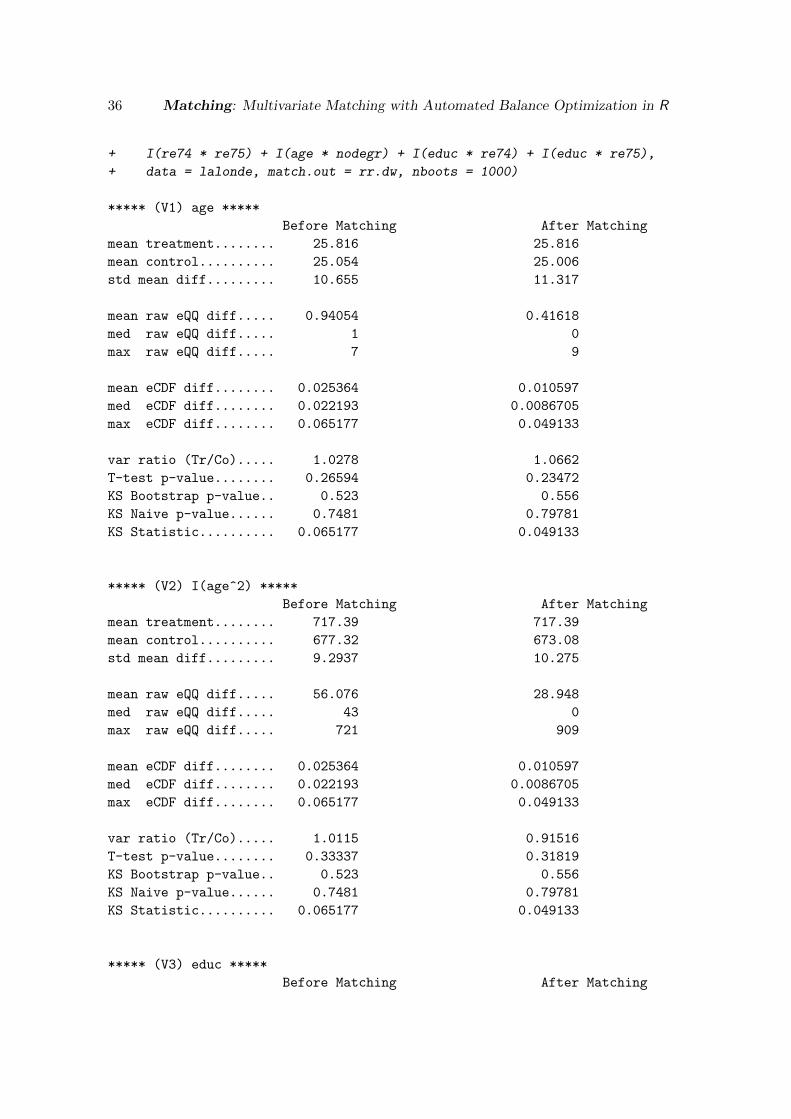
36 Matching: Multivariate Matching with Automated Balance Optimization in R
+ I(re74 * re75) + I(age * nodegr) + I(educ * re74) + I(educ * re75),
+ data = lalonde, match.out = rr.dw, nboots = 1000)
***** (V1) age *****
Before Matching After Matching
mean treatment........ 25.816 25.816
mean control.......... 25.054 25.006
std mean diff......... 10.655 11.317
mean raw eQQ diff..... 0.94054 0.41618
med raw eQQ diff..... 1 0
max raw eQQ diff..... 7 9
mean eCDF diff........ 0.025364 0.010597
med eCDF diff........ 0.022193 0.0086705
max eCDF diff........ 0.065177 0.049133
var ratio (Tr/Co)..... 1.0278 1.0662
T-test p-value........ 0.26594 0.23472
KS Bootstrap p-value.. 0.523 0.556
KS Naive p-value...... 0.7481 0.79781
KS Statistic.......... 0.065177 0.049133
***** (V2) I(age^2) *****
Before Matching After Matching
mean treatment........ 717.39 717.39
mean control.......... 677.32 673.08
std mean diff......... 9.2937 10.275
mean raw eQQ diff..... 56.076 28.948
med raw eQQ diff..... 43 0
max raw eQQ diff..... 721 909
mean eCDF diff........ 0.025364 0.010597
med eCDF diff........ 0.022193 0.0086705
max eCDF diff........ 0.065177 0.049133
var ratio (Tr/Co)..... 1.0115 0.91516
T-test p-value........ 0.33337 0.31819
KS Bootstrap p-value.. 0.523 0.556
KS Naive p-value...... 0.7481 0.79781
KS Statistic.......... 0.065177 0.049133
***** (V3) educ *****
Before Matching After Matching
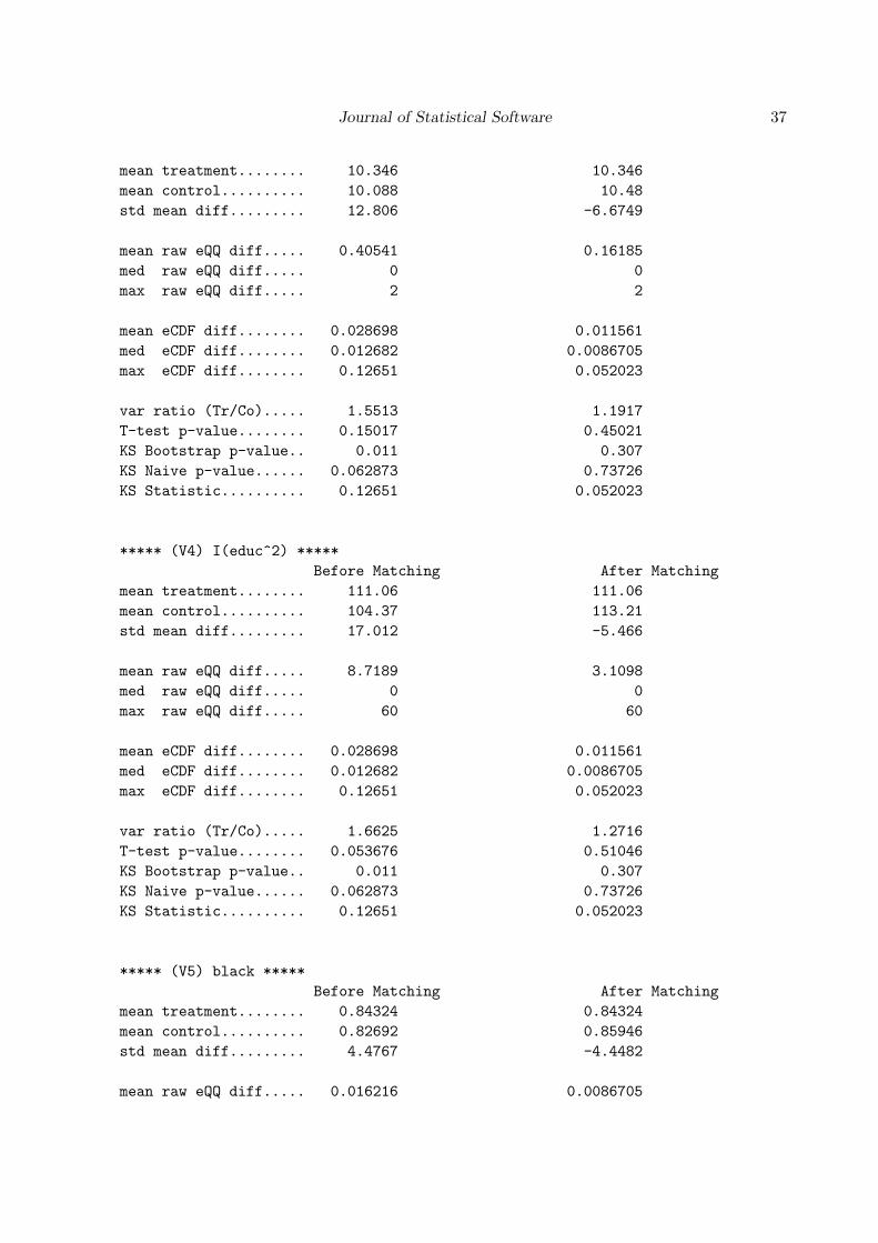
Journal of Statistical Software 37
mean treatment........ 10.346 10.346
mean control.......... 10.088 10.48
std mean diff......... 12.806 -6.6749
mean raw eQQ diff..... 0.40541 0.16185
med raw eQQ diff..... 0 0
max raw eQQ diff..... 2 2
mean eCDF diff........ 0.028698 0.011561
med eCDF diff........ 0.012682 0.0086705
max eCDF diff........ 0.12651 0.052023
var ratio (Tr/Co)..... 1.5513 1.1917
T-test p-value........ 0.15017 0.45021
KS Bootstrap p-value.. 0.011 0.307
KS Naive p-value...... 0.062873 0.73726
KS Statistic.......... 0.12651 0.052023
***** (V4) I(educ^2) *****
Before Matching After Matching
mean treatment........ 111.06 111.06
mean control.......... 104.37 113.21
std mean diff......... 17.012 -5.466
mean raw eQQ diff..... 8.7189 3.1098
med raw eQQ diff..... 0 0
max raw eQQ diff..... 60 60
mean eCDF diff........ 0.028698 0.011561
med eCDF diff........ 0.012682 0.0086705
max eCDF diff........ 0.12651 0.052023
var ratio (Tr/Co)..... 1.6625 1.2716
T-test p-value........ 0.053676 0.51046
KS Bootstrap p-value.. 0.011 0.307
KS Naive p-value...... 0.062873 0.73726
KS Statistic.......... 0.12651 0.052023
***** (V5) black *****
Before Matching After Matching
mean treatment........ 0.84324 0.84324
mean control.......... 0.82692 0.85946
std mean diff......... 4.4767 -4.4482
mean raw eQQ diff..... 0.016216 0.0086705
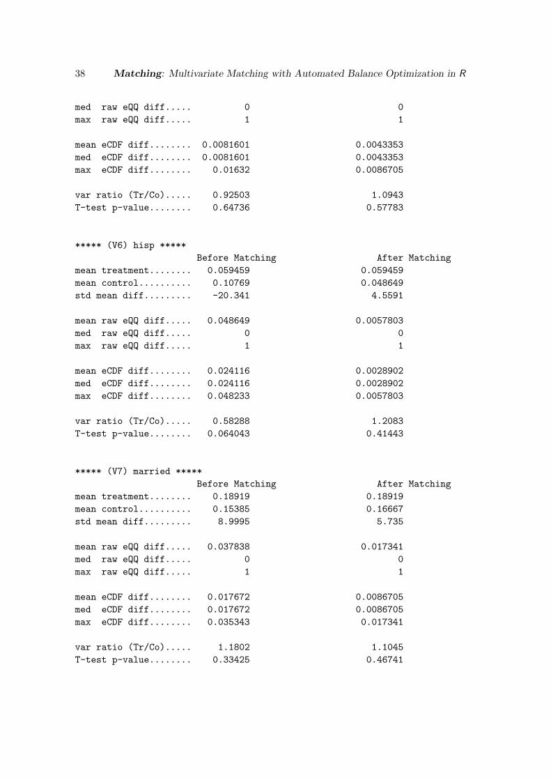
38 Matching: Multivariate Matching with Automated Balance Optimization in R
med raw eQQ diff..... 0 0
max raw eQQ diff..... 1 1
mean eCDF diff........ 0.0081601 0.0043353
med eCDF diff........ 0.0081601 0.0043353
max eCDF diff........ 0.01632 0.0086705
var ratio (Tr/Co)..... 0.92503 1.0943
T-test p-value........ 0.64736 0.57783
***** (V6) hisp *****
Before Matching After Matching
mean treatment........ 0.059459 0.059459
mean control.......... 0.10769 0.048649
std mean diff......... -20.341 4.5591
mean raw eQQ diff..... 0.048649 0.0057803
med raw eQQ diff..... 0 0
max raw eQQ diff..... 1 1
mean eCDF diff........ 0.024116 0.0028902
med eCDF diff........ 0.024116 0.0028902
max eCDF diff........ 0.048233 0.0057803
var ratio (Tr/Co)..... 0.58288 1.2083
T-test p-value........ 0.064043 0.41443
***** (V7) married *****
Before Matching After Matching
mean treatment........ 0.18919 0.18919
mean control.......... 0.15385 0.16667
std mean diff......... 8.9995 5.735
mean raw eQQ diff..... 0.037838 0.017341
med raw eQQ diff..... 0 0
max raw eQQ diff..... 1 1
mean eCDF diff........ 0.017672 0.0086705
med eCDF diff........ 0.017672 0.0086705
max eCDF diff........ 0.035343 0.017341
var ratio (Tr/Co)..... 1.1802 1.1045
T-test p-value........ 0.33425 0.46741
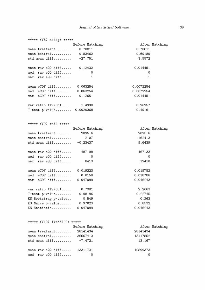
Journal of Statistical Software 39
***** (V8) nodegr *****
Before Matching After Matching
mean treatment........ 0.70811 0.70811
mean control.......... 0.83462 0.69189
std mean diff......... -27.751 3.5572
mean raw eQQ diff..... 0.12432 0.014451
med raw eQQ diff..... 0 0
max raw eQQ diff..... 1 1
mean eCDF diff........ 0.063254 0.0072254
med eCDF diff........ 0.063254 0.0072254
max eCDF diff........ 0.12651 0.014451
var ratio (Tr/Co)..... 1.4998 0.96957
T-test p-value........ 0.0020368 0.49161
***** (V9) re74 *****
Before Matching After Matching
mean treatment........ 2095.6 2095.6
mean control.......... 2107 1624.3
std mean diff......... -0.23437 9.6439
mean raw eQQ diff..... 487.98 467.33
med raw eQQ diff..... 0 0
max raw eQQ diff..... 8413 12410
mean eCDF diff........ 0.019223 0.019782
med eCDF diff........ 0.0158 0.018786
max eCDF diff........ 0.047089 0.046243
var ratio (Tr/Co)..... 0.7381 2.2663
T-test p-value........ 0.98186 0.22745
KS Bootstrap p-value.. 0.549 0.263
KS Naive p-value...... 0.97023 0.8532
KS Statistic.......... 0.047089 0.046243
***** (V10) I(re74^2) *****
Before Matching After Matching
mean treatment........ 28141434 28141434
mean control.......... 36667413 13117852
std mean diff......... -7.4721 13.167
mean raw eQQ diff..... 13311731 10899373
med raw eQQ diff..... 0 0
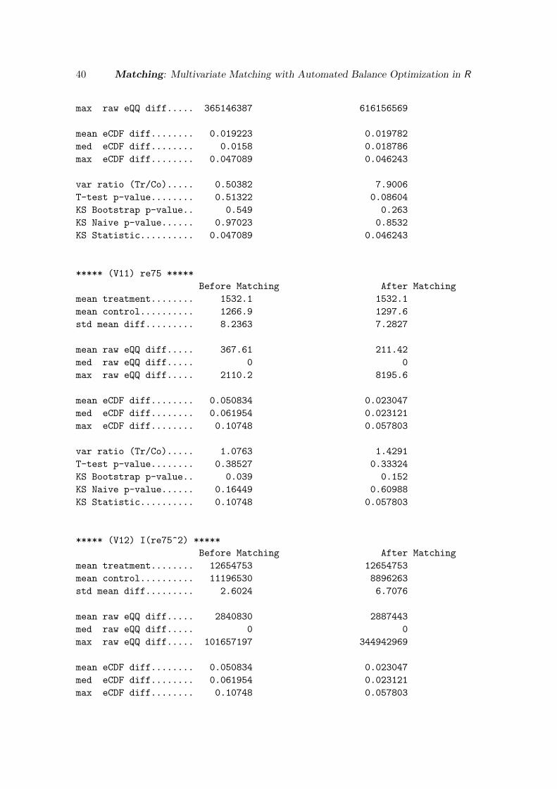
40 Matching: Multivariate Matching with Automated Balance Optimization in R
max raw eQQ diff..... 365146387 616156569
mean eCDF diff........ 0.019223 0.019782
med eCDF diff........ 0.0158 0.018786
max eCDF diff........ 0.047089 0.046243
var ratio (Tr/Co)..... 0.50382 7.9006
T-test p-value........ 0.51322 0.08604
KS Bootstrap p-value.. 0.549 0.263
KS Naive p-value...... 0.97023 0.8532
KS Statistic.......... 0.047089 0.046243
***** (V11) re75 *****
Before Matching After Matching
mean treatment........ 1532.1 1532.1
mean control.......... 1266.9 1297.6
std mean diff......... 8.2363 7.2827
mean raw eQQ diff..... 367.61 211.42
med raw eQQ diff..... 0 0
max raw eQQ diff..... 2110.2 8195.6
mean eCDF diff........ 0.050834 0.023047
med eCDF diff........ 0.061954 0.023121
max eCDF diff........ 0.10748 0.057803
var ratio (Tr/Co)..... 1.0763 1.4291
T-test p-value........ 0.38527 0.33324
KS Bootstrap p-value.. 0.039 0.152
KS Naive p-value...... 0.16449 0.60988
KS Statistic.......... 0.10748 0.057803
***** (V12) I(re75^2) *****
Before Matching After Matching
mean treatment........ 12654753 12654753
mean control.......... 11196530 8896263
std mean diff......... 2.6024 6.7076
mean raw eQQ diff..... 2840830 2887443
med raw eQQ diff..... 0 0
max raw eQQ diff..... 101657197 344942969
mean eCDF diff........ 0.050834 0.023047
med eCDF diff........ 0.061954 0.023121
max eCDF diff........ 0.10748 0.057803

Journal of Statistical Software 41
var ratio (Tr/Co)..... 1.4609 3.559
T-test p-value........ 0.77178 0.37741
KS Bootstrap p-value.. 0.039 0.152
KS Naive p-value...... 0.16449 0.60988
KS Statistic.......... 0.10748 0.057803
***** (V13) u74 *****
Before Matching After Matching
mean treatment........ 0.70811 0.70811
mean control.......... 0.75 0.68458
std mean diff......... -9.1895 5.1608
mean raw eQQ diff..... 0.037838 0.017341
med raw eQQ diff..... 0 0
max raw eQQ diff..... 1 1
mean eCDF diff........ 0.020946 0.0086705
med eCDF diff........ 0.020946 0.0086705
max eCDF diff........ 0.041892 0.017341
var ratio (Tr/Co)..... 1.1041 0.95721
T-test p-value........ 0.33033 0.52298
***** (V14) u75 *****
Before Matching After Matching
mean treatment........ 0.6 0.6
mean control.......... 0.68462 0.62072
std mean diff......... -17.225 -4.2182
mean raw eQQ diff..... 0.081081 0.031792
med raw eQQ diff..... 0 0
max raw eQQ diff..... 1 1
mean eCDF diff........ 0.042308 0.015896
med eCDF diff........ 0.042308 0.015896
max eCDF diff........ 0.084615 0.031792
var ratio (Tr/Co)..... 1.1133 1.0194
T-test p-value........ 0.068031 0.46507
***** (V15) I(re74 * re75) *****
Before Matching After Matching
mean treatment........ 13118591 13118591
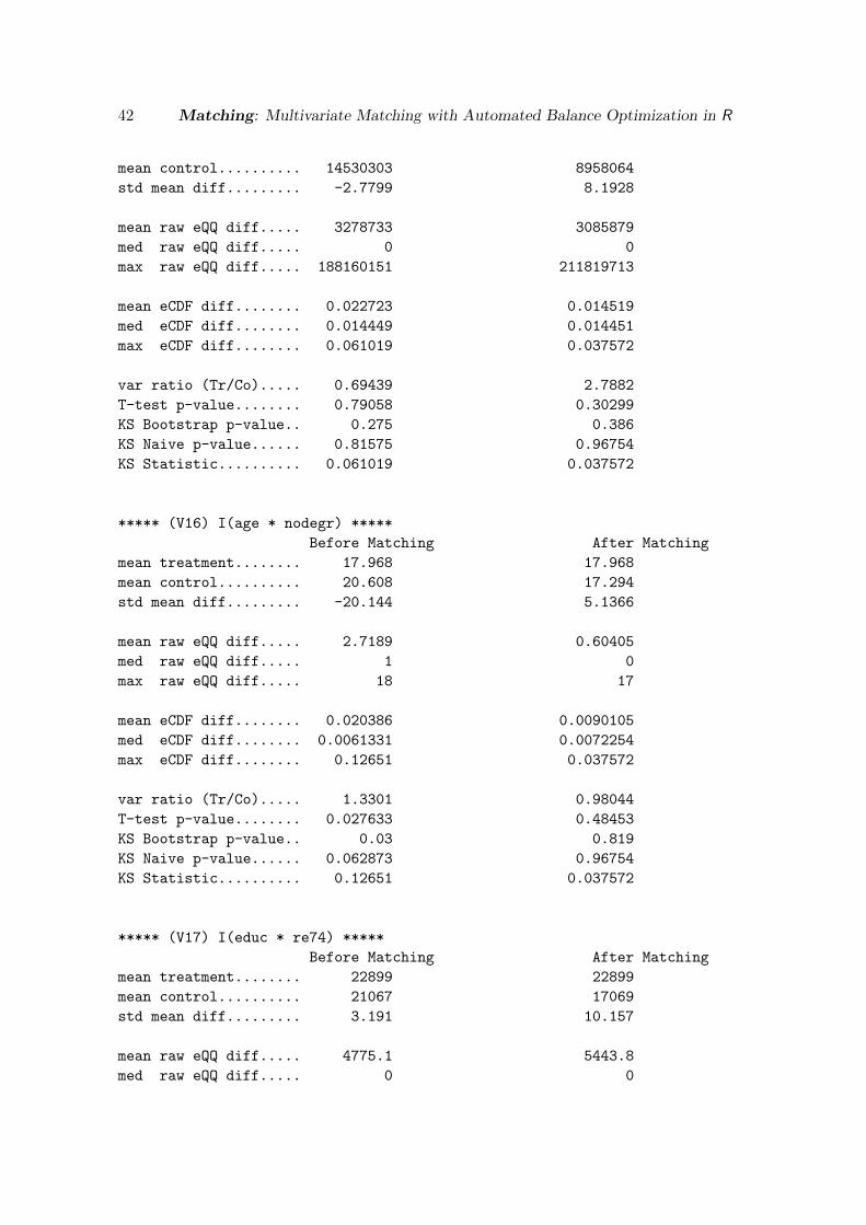
42 Matching: Multivariate Matching with Automated Balance Optimization in R
mean control.......... 14530303 8958064
std mean diff......... -2.7799 8.1928
mean raw eQQ diff..... 3278733 3085879
med raw eQQ diff..... 0 0
max raw eQQ diff..... 188160151 211819713
mean eCDF diff........ 0.022723 0.014519
med eCDF diff........ 0.014449 0.014451
max eCDF diff........ 0.061019 0.037572
var ratio (Tr/Co)..... 0.69439 2.7882
T-test p-value........ 0.79058 0.30299
KS Bootstrap p-value.. 0.275 0.386
KS Naive p-value...... 0.81575 0.96754
KS Statistic.......... 0.061019 0.037572
***** (V16) I(age * nodegr) *****
Before Matching After Matching
mean treatment........ 17.968 17.968
mean control.......... 20.608 17.294
std mean diff......... -20.144 5.1366
mean raw eQQ diff..... 2.7189 0.60405
med raw eQQ diff..... 1 0
max raw eQQ diff..... 18 17
mean eCDF diff........ 0.020386 0.0090105
med eCDF diff........ 0.0061331 0.0072254
max eCDF diff........ 0.12651 0.037572
var ratio (Tr/Co)..... 1.3301 0.98044
T-test p-value........ 0.027633 0.48453
KS Bootstrap p-value.. 0.03 0.819
KS Naive p-value...... 0.062873 0.96754
KS Statistic.......... 0.12651 0.037572
***** (V17) I(educ * re74) *****
Before Matching After Matching
mean treatment........ 22899 22899
mean control.......... 21067 17069
std mean diff......... 3.191 10.157
mean raw eQQ diff..... 4775.1 5443.8
med raw eQQ diff..... 0 0
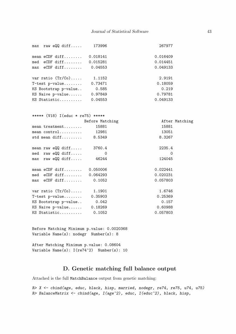
Journal of Statistical Software 43
max raw eQQ diff..... 173996 267977
mean eCDF diff........ 0.018141 0.016409
med eCDF diff........ 0.015281 0.014451
max eCDF diff........ 0.04553 0.049133
var ratio (Tr/Co)..... 1.1152 2.9191
T-test p-value........ 0.73471 0.18059
KS Bootstrap p-value.. 0.585 0.219
KS Naive p-value...... 0.97849 0.79781
KS Statistic.......... 0.04553 0.049133
***** (V18) I(educ * re75) *****
Before Matching After Matching
mean treatment........ 15881 15881
mean control.......... 12981 13051
std mean diff......... 8.5349 8.3267
mean raw eQQ diff..... 3760.4 2235.4
med raw eQQ diff..... 0 0
max raw eQQ diff..... 46244 124045
mean eCDF diff........ 0.050006 0.022441
med eCDF diff........ 0.064293 0.020231
max eCDF diff........ 0.1052 0.057803
var ratio (Tr/Co)..... 1.1901 1.6746
T-test p-value........ 0.35903 0.25369
KS Bootstrap p-value.. 0.042 0.157
KS Naive p-value...... 0.18269 0.60988
KS Statistic.......... 0.1052 0.057803
Before Matching Minimum p.value: 0.0020368
Variable Name(s): nodegr Number(s): 8
After Matching Minimum p.value: 0.08604
Variable Name(s): I(re74^2) Number(s): 10
D. Genetic matching full balance output
Attached is the full MatchBalance output from genetic matching:
R> X <- cbind(age, educ, black, hisp, married, nodegr, re74, re75, u74, u75)
R> BalanceMatrix <- cbind(age, I(age^2), educ, I(educ^2), black, hisp,
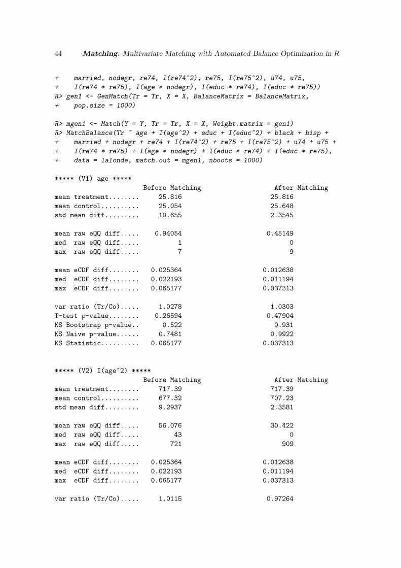
44 Matching: Multivariate Matching with Automated Balance Optimization in R
+ married, nodegr, re74, I(re74^2), re75, I(re75^2), u74, u75,
+ I(re74 * re75), I(age * nodegr), I(educ * re74), I(educ * re75))
R> gen1 <- GenMatch(Tr = Tr, X = X, BalanceMatrix = BalanceMatrix,
+ pop.size = 1000)
R> mgen1 <- Match(Y = Y, Tr = Tr, X = X, Weight.matrix = gen1)
R> MatchBalance(Tr ~ age + I(age^2) + educ + I(educ^2) + black + hisp +
+ married + nodegr + re74 + I(re74^2) + re75 + I(re75^2) + u74 + u75 +
+ I(re74 * re75) + I(age * nodegr) + I(educ * re74) + I(educ * re75),
+ data = lalonde, match.out = mgen1, nboots = 1000)
***** (V1) age *****
Before Matching After Matching
mean treatment........ 25.816 25.816
mean control.......... 25.054 25.648
std mean diff......... 10.655 2.3545
mean raw eQQ diff..... 0.94054 0.45149
med raw eQQ diff..... 1 0
max raw eQQ diff..... 7 9
mean eCDF diff........ 0.025364 0.012638
med eCDF diff........ 0.022193 0.011194
max eCDF diff........ 0.065177 0.037313
var ratio (Tr/Co)..... 1.0278 1.0303
T-test p-value........ 0.26594 0.47904
KS Bootstrap p-value.. 0.522 0.931
KS Naive p-value...... 0.7481 0.9922
KS Statistic.......... 0.065177 0.037313
***** (V2) I(age^2) *****
Before Matching After Matching
mean treatment........ 717.39 717.39
mean control.......... 677.32 707.23
std mean diff......... 9.2937 2.3581
mean raw eQQ diff..... 56.076 30.422
med raw eQQ diff..... 43 0
max raw eQQ diff..... 721 909
mean eCDF diff........ 0.025364 0.012638
med eCDF diff........ 0.022193 0.011194
max eCDF diff........ 0.065177 0.037313
var ratio (Tr/Co)..... 1.0115 0.97264
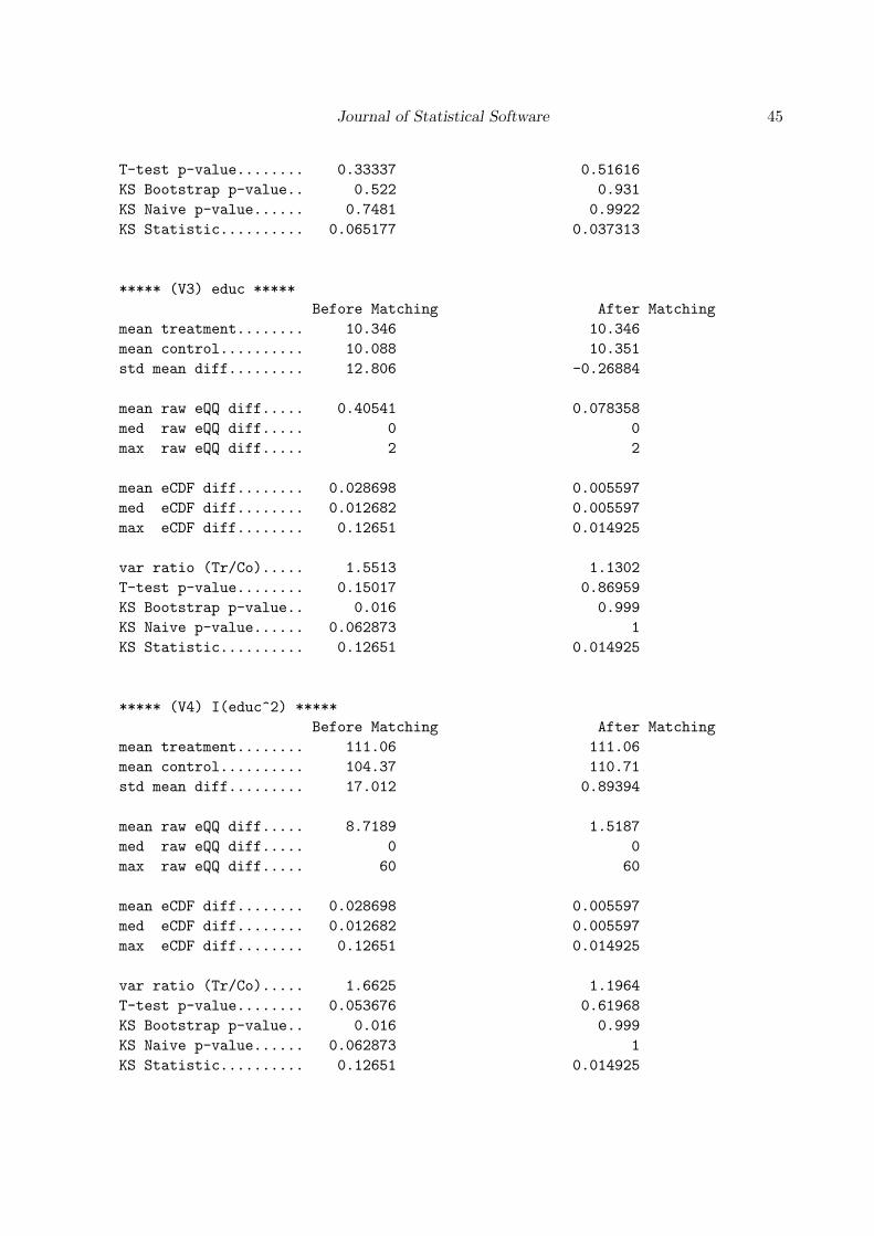
Journal of Statistical Software 45
T-test p-value........ 0.33337 0.51616
KS Bootstrap p-value.. 0.522 0.931
KS Naive p-value...... 0.7481 0.9922
KS Statistic.......... 0.065177 0.037313
***** (V3) educ *****
Before Matching After Matching
mean treatment........ 10.346 10.346
mean control.......... 10.088 10.351
std mean diff......... 12.806 -0.26884
mean raw eQQ diff..... 0.40541 0.078358
med raw eQQ diff..... 0 0
max raw eQQ diff..... 2 2
mean eCDF diff........ 0.028698 0.005597
med eCDF diff........ 0.012682 0.005597
max eCDF diff........ 0.12651 0.014925
var ratio (Tr/Co)..... 1.5513 1.1302
T-test p-value........ 0.15017 0.86959
KS Bootstrap p-value.. 0.016 0.999
KS Naive p-value...... 0.062873 1
KS Statistic.......... 0.12651 0.014925
***** (V4) I(educ^2) *****
Before Matching After Matching
mean treatment........ 111.06 111.06
mean control.......... 104.37 110.71
std mean diff......... 17.012 0.89394
mean raw eQQ diff..... 8.7189 1.5187
med raw eQQ diff..... 0 0
max raw eQQ diff..... 60 60
mean eCDF diff........ 0.028698 0.005597
med eCDF diff........ 0.012682 0.005597
max eCDF diff........ 0.12651 0.014925
var ratio (Tr/Co)..... 1.6625 1.1964
T-test p-value........ 0.053676 0.61968
KS Bootstrap p-value.. 0.016 0.999
KS Naive p-value...... 0.062873 1
KS Statistic.......... 0.12651 0.014925
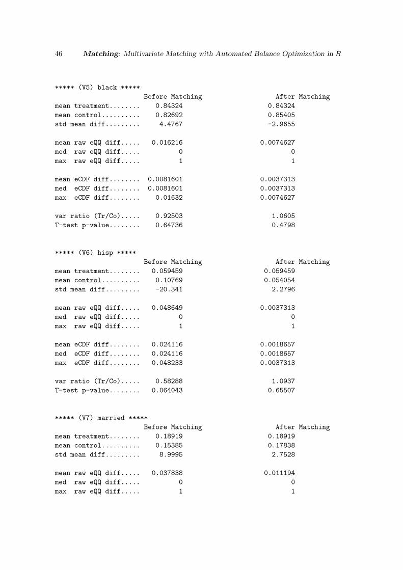
46 Matching: Multivariate Matching with Automated Balance Optimization in R
***** (V5) black *****
Before Matching After Matching
mean treatment........ 0.84324 0.84324
mean control.......... 0.82692 0.85405
std mean diff......... 4.4767 -2.9655
mean raw eQQ diff..... 0.016216 0.0074627
med raw eQQ diff..... 0 0
max raw eQQ diff..... 1 1
mean eCDF diff........ 0.0081601 0.0037313
med eCDF diff........ 0.0081601 0.0037313
max eCDF diff........ 0.01632 0.0074627
var ratio (Tr/Co)..... 0.92503 1.0605
T-test p-value........ 0.64736 0.4798
***** (V6) hisp *****
Before Matching After Matching
mean treatment........ 0.059459 0.059459
mean control.......... 0.10769 0.054054
std mean diff......... -20.341 2.2796
mean raw eQQ diff..... 0.048649 0.0037313
med raw eQQ diff..... 0 0
max raw eQQ diff..... 1 1
mean eCDF diff........ 0.024116 0.0018657
med eCDF diff........ 0.024116 0.0018657
max eCDF diff........ 0.048233 0.0037313
var ratio (Tr/Co)..... 0.58288 1.0937
T-test p-value........ 0.064043 0.65507
***** (V7) married *****
Before Matching After Matching
mean treatment........ 0.18919 0.18919
mean control.......... 0.15385 0.17838
std mean diff......... 8.9995 2.7528
mean raw eQQ diff..... 0.037838 0.011194
med raw eQQ diff..... 0 0
max raw eQQ diff..... 1 1
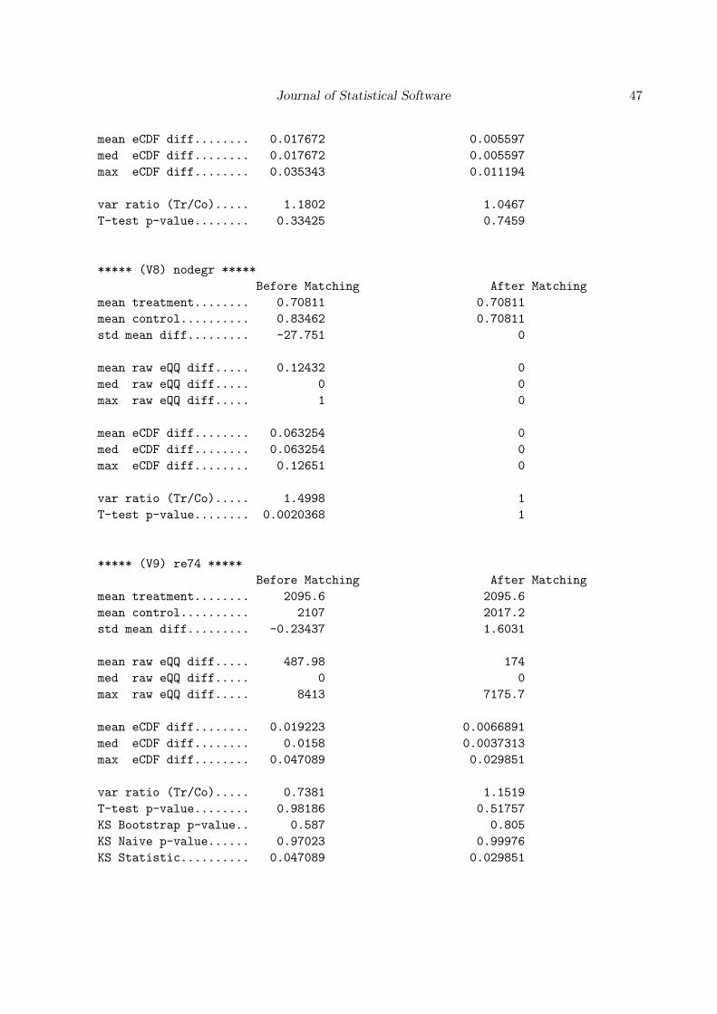
Journal of Statistical Software 47
mean eCDF diff........ 0.017672 0.005597
med eCDF diff........ 0.017672 0.005597
max eCDF diff........ 0.035343 0.011194
var ratio (Tr/Co)..... 1.1802 1.0467
T-test p-value........ 0.33425 0.7459
***** (V8) nodegr *****
Before Matching After Matching
mean treatment........ 0.70811 0.70811
mean control.......... 0.83462 0.70811
std mean diff......... -27.751 0
mean raw eQQ diff..... 0.12432 0
med raw eQQ diff..... 0 0
max raw eQQ diff..... 1 0
mean eCDF diff........ 0.063254 0
med eCDF diff........ 0.063254 0
max eCDF diff........ 0.12651 0
var ratio (Tr/Co)..... 1.4998 1
T-test p-value........ 0.0020368 1
***** (V9) re74 *****
Before Matching After Matching
mean treatment........ 2095.6 2095.6
mean control.......... 2107 2017.2
std mean diff......... -0.23437 1.6031
mean raw eQQ diff..... 487.98 174
med raw eQQ diff..... 0 0
max raw eQQ diff..... 8413 7175.7
mean eCDF diff........ 0.019223 0.0066891
med eCDF diff........ 0.0158 0.0037313
max eCDF diff........ 0.047089 0.029851
var ratio (Tr/Co)..... 0.7381 1.1519
T-test p-value........ 0.98186 0.51757
KS Bootstrap p-value.. 0.587 0.805
KS Naive p-value...... 0.97023 0.99976
KS Statistic.......... 0.047089 0.029851

48 Matching: Multivariate Matching with Automated Balance Optimization in R
***** (V10) I(re74^2) *****
Before Matching After Matching
mean treatment........ 28141434 28141434
mean control.......... 36667413 24686484
std mean diff......... -7.4721 3.0279
mean raw eQQ diff..... 13311731 4823772
med raw eQQ diff..... 0 0
max raw eQQ diff..... 365146387 451383821
mean eCDF diff........ 0.019223 0.0066891
med eCDF diff........ 0.0158 0.0037313
max eCDF diff........ 0.047089 0.029851
var ratio (Tr/Co)..... 0.50382 1.5233
T-test p-value........ 0.51322 0.4652
KS Bootstrap p-value.. 0.587 0.805
KS Naive p-value...... 0.97023 0.99976
KS Statistic.......... 0.047089 0.029851
***** (V11) re75 *****
Before Matching After Matching
mean treatment........ 1532.1 1532.1
mean control.......... 1266.9 1483
std mean diff......... 8.2363 1.5234
mean raw eQQ diff..... 367.61 167.61
med raw eQQ diff..... 0 0
max raw eQQ diff..... 2110.2 2973.4
mean eCDF diff........ 0.050834 0.016297
med eCDF diff........ 0.061954 0.014925
max eCDF diff........ 0.10748 0.044776
var ratio (Tr/Co)..... 1.0763 1.0405
T-test p-value........ 0.38527 0.63214
KS Bootstrap p-value.. 0.043 0.563
KS Naive p-value...... 0.16449 0.951
KS Statistic.......... 0.10748 0.044776
***** (V12) I(re75^2) *****
Before Matching After Matching
mean treatment........ 12654753 12654753
mean control.......... 11196530 12106082
std mean diff......... 2.6024 0.97918

Journal of Statistical Software 49
mean raw eQQ diff..... 2840830 2124586
med raw eQQ diff..... 0 0
max raw eQQ diff..... 101657197 101657197
mean eCDF diff........ 0.050834 0.016297
med eCDF diff........ 0.061954 0.014925
max eCDF diff........ 0.10748 0.044776
var ratio (Tr/Co)..... 1.4609 1.3641
T-test p-value........ 0.77178 0.69082
KS Bootstrap p-value.. 0.043 0.563
KS Naive p-value...... 0.16449 0.951
KS Statistic.......... 0.10748 0.044776
***** (V13) u74 *****
Before Matching After Matching
mean treatment........ 0.70811 0.70811
mean control.......... 0.75 0.70811
std mean diff......... -9.1895 0
mean raw eQQ diff..... 0.037838 0
med raw eQQ diff..... 0 0
max raw eQQ diff..... 1 0
mean eCDF diff........ 0.020946 0
med eCDF diff........ 0.020946 0
max eCDF diff........ 0.041892 0
var ratio (Tr/Co)..... 1.1041 1
T-test p-value........ 0.33033 1
***** (V14) u75 *****
Before Matching After Matching
mean treatment........ 0.6 0.6
mean control.......... 0.68462 0.61622
std mean diff......... -17.225 -3.3012
mean raw eQQ diff..... 0.081081 0.018657
med raw eQQ diff..... 0 0
max raw eQQ diff..... 1 1
mean eCDF diff........ 0.042308 0.0093284
med eCDF diff........ 0.042308 0.0093284
max eCDF diff........ 0.084615 0.018657
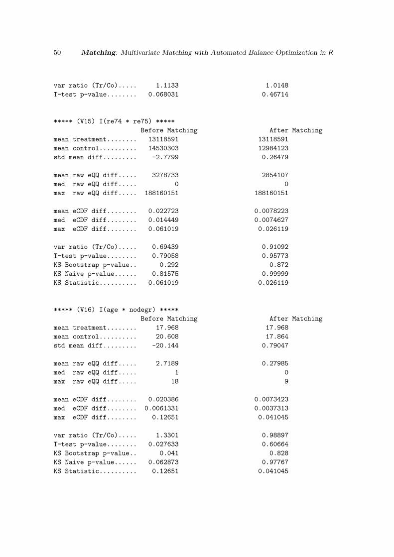
50 Matching: Multivariate Matching with Automated Balance Optimization in R
var ratio (Tr/Co)..... 1.1133 1.0148
T-test p-value........ 0.068031 0.46714
***** (V15) I(re74 * re75) *****
Before Matching After Matching
mean treatment........ 13118591 13118591
mean control.......... 14530303 12984123
std mean diff......... -2.7799 0.26479
mean raw eQQ diff..... 3278733 2854107
med raw eQQ diff..... 0 0
max raw eQQ diff..... 188160151 188160151
mean eCDF diff........ 0.022723 0.0078223
med eCDF diff........ 0.014449 0.0074627
max eCDF diff........ 0.061019 0.026119
var ratio (Tr/Co)..... 0.69439 0.91092
T-test p-value........ 0.79058 0.95773
KS Bootstrap p-value.. 0.292 0.872
KS Naive p-value...... 0.81575 0.99999
KS Statistic.......... 0.061019 0.026119
***** (V16) I(age * nodegr) *****
Before Matching After Matching
mean treatment........ 17.968 17.968
mean control.......... 20.608 17.864
std mean diff......... -20.144 0.79047
mean raw eQQ diff..... 2.7189 0.27985
med raw eQQ diff..... 1 0
max raw eQQ diff..... 18 9
mean eCDF diff........ 0.020386 0.0073423
med eCDF diff........ 0.0061331 0.0037313
max eCDF diff........ 0.12651 0.041045
var ratio (Tr/Co)..... 1.3301 0.98897
T-test p-value........ 0.027633 0.60664
KS Bootstrap p-value.. 0.041 0.828
KS Naive p-value...... 0.062873 0.97767
KS Statistic.......... 0.12651 0.041045

Journal of Statistical Software 51
***** (V17) I(educ * re74) *****
Before Matching After Matching
mean treatment........ 22899 22899
mean control.......... 21067 21615
std mean diff......... 3.191 2.236
mean raw eQQ diff..... 4775.1 2863.8
med raw eQQ diff..... 0 0
max raw eQQ diff..... 173996 211917
mean eCDF diff........ 0.018141 0.0075061
med eCDF diff........ 0.015281 0.0074627
max eCDF diff........ 0.04553 0.026119
var ratio (Tr/Co)..... 1.1152 1.3621
T-test p-value........ 0.73471 0.40827
KS Bootstrap p-value.. 0.632 0.876
KS Naive p-value...... 0.97849 0.99999
KS Statistic.......... 0.04553 0.026119
***** (V18) I(educ * re75) *****
Before Matching After Matching
mean treatment........ 15881 15881
mean control.......... 12981 15521
std mean diff......... 8.5349 1.0583
mean raw eQQ diff..... 3760.4 1949.2
med raw eQQ diff..... 0 0
max raw eQQ diff..... 46244 46244
mean eCDF diff........ 0.050006 0.01618
med eCDF diff........ 0.064293 0.014925
max eCDF diff........ 0.1052 0.041045
var ratio (Tr/Co)..... 1.1901 1.0948
T-test p-value........ 0.35903 0.76596
KS Bootstrap p-value.. 0.052 0.652
KS Naive p-value...... 0.18269 0.97767
KS Statistic.......... 0.1052 0.041045
Before Matching Minimum p.value: 0.0020368
Variable Name(s): nodegr Number(s): 8
After Matching Minimum p.value: 0.40827
Variable Name(s): I(educ * re74) Number(s): 17

52 Matching: Multivariate Matching with Automated Balance Optimization in R
Affiliation:
Jasjeet S. SekhonDepartment of Political Science210 Barrows Hall #1950UC BerkeleyBerkeley, CA 94720-1950, United States of AmericaE-mail: [email protected]: http://sekhon.berkeley.edu
Journal of Statistical Software http://www.jstatsoft.org/
published by the American Statistical Association http://www.amstat.org/
Volume 42, Issue 7 Submitted: 2007-02-07May 2011 Accepted: 2007-06-18