multitarget tracking using the joint multitarget...

Multitarget Tracking using theJoint Multitarget ProbabilityDensity

CHRIS KREUCHER

KEITH KASTELLAGeneral Dynamics Advanced Information Systems

ALFRED O. HERO, III, Fellow, IEEEUniversity of Michigan

This work addresses the problem of tracking multiple moving

targets by recursively estimating the joint multitarget probability

density (JMPD). Estimation of the JMPD is done in a Bayesian

framework and provides a method for tracking multiple targets

which allows nonlinear target motion and measurement to state

coupling as well as non-Gaussian target state densities. The JMPD

technique simultaneously estimates both the target states and the

number of targets in the surveillance region based on the set of

measurements made. We give an implementation of the JMPD

method based on particle filtering techniques and provide an

adaptive sampling scheme which explicitly models the multitarget

nature of the problem. We show that this implementation of the

JMPD technique provides a natural way to track a collection of

targets, is computationally tractable, and performs well under

difficult conditions such as target crossing, convoy movement, and

low measurement signal-to-noise ratio (SNR).

Manuscript received December 10, 2003; revised May 3 and July20, 2004; released for publication March 19, 2005.

IEEE Log No. T-AES/41/4/860802.

Refereeing of this contribution was handled by W. Koch.

This work was supported under the United States Air ForceContract F33615-02-C-1199, AFRL Contract SPO900-96-D-0080,and by ARO-DARPA MURI Grant DAAD19-02-1-0262. Anyopinions, findings and conclusions, or recommendations expressedin this material are those of the authors and do not necessarilyreflect the views of the United States Air Force.

Authors’ addresses: C. Kreucher and K. Kastella, GeneralDynamics, 1200 Joe Hall Dr., Ypsilanti, MI 48197, E-mail:([email protected]); A. O. Hero, III, Dept. ofElectrical and Computer Engineering, University of Michigan, 1301Beal Ave., Ann Arbor, MI 48109-2122.

0018-9251/05/$17.00 c° 2005 IEEE

I. INTRODUCTION

The problem of tracking a single maneuveringtarget in a cluttered environment is a very well-studiedarea [4]. Normally, the objective is to predict the stateof an object based on a set of noisy and ambiguousmeasurements. There are wide range of applications inwhich the target tracking problem arises, includingvehicle collision warning and avoidance [39, 17],mobile robotics [50], human-computer interaction[24], speaker localization [66], animal tracking [65],tracking a person [11], and tracking a military targetsuch as a ship, aircraft, or tank [8].The single target tracking problem can be

formulated and solved in a Bayesian setting byrepresenting the target state probabilistically andincorporating statistical models for the sensing actionand the target state transition. Implementationally, thestandard tool is the ubiquitous Kalman filter [46],applicable and optimal when the measurement andstate dynamics are Gaussian and linear.In a more general setting where nonlinear target

motions, non-Gaussian densities, or nonlinearmeasurement-to-target couplings are involved, moresophisticated nonlinear filtering techniques arenecessary [3]. Standard nonlinear filtering techniquesinvolve modifications to the Kalman filter such as theextended Kalman filter [26], the unscented Kalmanfilter [27], and Gaussian sum approximations [1],all of which relax some of the linearity assumptionspresent in the Kalman filter. However, thesetechniques do not accurately model all of the salientfeatures of the density, which limits their applicabilityto scenarios where the target state posterior densityis well approximated by a multivariate Gaussiandensity. To address this deficiency, others havestudied grid-based approaches [35, 37], which utilizea discrete representation of the entire single targetdensity. In this setup, no assumptions on the form ofthe density are required, so arbitrarily complicateddensities may be accommodated. However, fixed gridapproaches are computationally intractable except inthe case of very low state space dimensionality [7].Recently, the interest of the tracking community

has turned to the set of Monte Carlo techniquesknown as particle filtering [19, 59]. A particle filterapproximates a probability density on a set of discretepoints, where the points are chosen dynamically viaimportance sampling. Particle filtering techniqueshave the advantage that they provide computationaltractability [51], have provable convergence properties[12], and are applicable under the most general ofcircumstances, as there is no assumption made onthe form of the density [15]. Indeed, particle filterbased approaches have been used successfully inareas where grid-based [13] or extended or unscentedKalman filter-based [2, 44] filters have previouslybeen employed.

1396 IEEE TRANSACTIONS ON AEROSPACE AND ELECTRONIC SYSTEMS VOL. 41, NO. 4 OCTOBER 2005

Authorized licensed use limited to: University of Michigan Library. Downloaded on May 5, 2009 at 16:01 from IEEE Xplore. Restrictions apply.

The multitarget tracking problem has beentraditionally addressed with techniques such asmultiple hypothesis tracking (MHT) and jointprobabilistic data association (JPDA) [8, 5, 6]. Bothtechniques work by translating a measurement ofthe surveillance area into a set of detections bythresholding. The detections are then either associatedwith existing tracks, used to create new tracks, ordeemed false alarms. Typically, Kalman-filter typealgorithms are used to update the existing trackswith the new measurements after association. Thechallenge, of course, is to determine the correctassociation between measurements and targets.Others have approached the problem from a

fully Bayesian perspective. Stone [61] develops amathematical theory of multiple target tracking froma Bayesian point of view. Srivistava, Miller [48], andKastella [32] did early work in this area. For the samereasons as the single target case, fixed grid approachesto multitarget tracking are very computationallychallenging.Recently, some researchers have applied

particle filter based strategies to the problem ofmultitarget tracking. In [22], Hue and Le Cadre usea particle filter based on the probabilistic multiplehypothesis tracker (PMHT) introduced by Streit [62].Considerable attention is given to dealing with themeasurement-to-target association issue. Others havedone work which amounts to a blend between JPDAand particle filtering [29, 10].The BraMBLe [25] system, the independent

partition particle filter (IPPF) of Orton and Fitzgerald[52] and the work of Maskell [45] consider multitargettracking via particle filtering from a purely Bayesianperspective. Measurement-to-target association is notdone explicitly; it is implicit within the Bayesianframework. This work has focused on a tractableimplementation of ideas in [61].Mahler [41, 18, 49, 42] has developed an approach

to multitarget tracking based on random sets called“finite-set statistics” (FISST). Recently, FISSThas been combined with particle filtering methodsfor multitarget tracking [67, 57]. To date, theseimplementations have been limited to small scaleproblems for computational reasons. While developedindependently [31]—[33], the JMPD method canbe derived using the mathematics of random setsand expressed in the FISST framework (see [49]).As discussed there, JMPD can be traced back tothe event-averaged maximum likelihood estimation(EAMLE) work of Kastella [31, 32] and many earlierworks, e.g. [28, 47, 56]. Although this paper is moresimply viewed as an application of the JMPD methoddeveloped in [31]—[33], it can also be viewed as anapplication of the FISST method in the setting of [49].The main contribution of this paper is the

development of a multiple target tracker thatrecursively estimates the entire joint multitarget

probability density (JMPD) using particle filteringmethods with adaptive sampling schemes. This isan expansion of our preliminary work which waspublished in [36]. In our formulation, we use oneparticle per scenario. That is, a particle encodes ahypothesis about the entire multitarget state–whichincludes the number of targets and the state (position,velocity, etc.) of each target. We demonstrate thatthe particle filter implementation of JMPD providesa natural way to track a collection of targets, iscomputationally tractable, and performs well underdifficult conditions such as target crossing andconvoy movement. The method avoids the need tocreate detections via thresholding and avoids directlyperforming measurement-to-track association. Themeasurement enters into the Bayesian formulationthrough its likelihood, which allows raw sensormeasurements to be utilized. This feature allows thetracker to perform well in the low signal-to-noise ratio(SNR) regime.These features distinguish the particle filter based

JMPD approach from traditional approaches of MHTand JPDA as well as the approaches of Hue [22, 23]and others [29, 55, 16], which require thresholdedmeasurements (detections) and a measurement-to-trackassociation procedure. Further, by estimating thejoint multitarget density rather than many singletarget densities, our method explicitly models targetcorrelations. By utilizing an adaptive sampling schemethat exploits independence when present, our methodbenefits from computational advantages as in [52].The rest of this paper is organized in the following

manner. In Section II, we introduce the notion of theJMPD and show how the rules of Bayesian filteringare applied to produce a recursive filtering procedure.We give the particle filter based estimation of theJMPD in Section III. We detail therein the adaptivesampling strategy applied to automatically factor theJMPD when targets are behaving independently, whileappropriately handling targets that are coupled. Thisautomatic factorization is key to the computationaltractability of this implementation. We furthermoredetail the permutation symmetry issue (present in allmultitarget tracking algoritms) and its manifestationin our particle filter estimation of the JMPD. InSection IV, we give simulation results detailing theperformance of the particle filter based multitargettracker proposed here. Finally, we conclude inSection V with a brief summary and discussion.

II. JOINT MULTITARGET PROBABILITY DENSITY

In this section, we introduce the details ofusing the JMPD for target tracking. The conceptof JMPD was discussed by Kastella [30] wherea method of tracking multiple targets that movebetween fixed discrete cells on a line was presented.We generalize the discussion to deal with targets

KREUCHER ET AL.: MULTITARGET TRACKING USING THE JOINT MULTITARGET PROBABILITY DENSITY 1397


that have N-dimensional continuous valued statevectors and arbitrary kinematics. In the trackingproblems considered here, we are interested intracking the position (x,y) and velocity ( _x, _y) ofmultiple targets. Each target is therefore described bythe four-dimensional state vector x= [x, _x,y, _y]. Bystraightforward extension, the individual state vectorsof the targets may be augmented to include things liketarget identification.Recursive estimation of the JMPD provides a

means for tracking an unknown number of targets in aBayesian setting. The statistical model employed usesthe joint multitarget conditional probability densityp(xk1,x

k2, : : : ,x

kT¡1,x

kT,T

k j Zk) as the probability densityfor exactly T targets with states xk1,x

k2, : : : ,x

kT¡1,x

kT

at time k based on a set of past observations Zk. Ingeneral, the number of targets T is a variable to beestimated simultaneously with the states of the Ttargets. The observation set Zk refers to the collectionof measurements up to and including time k, i.e.,Zk = fz1,z2, : : : ,zkg, where each of the zi may be asingle measurement or a vector of measurements madeat time i.Each of the state vectors xt in the density

p(xk1,xk2, : : : ,x

kT¡1,x

kT,T

k j Zk) is a vector quantityand may (for example) be of the form [x, _x,y, _y].We refer to each of the T target state vectorsx1,x2, : : : ,xT¡1,xT as a partition of the multitargetstate X. For convenience, the density is written morecompactly in the traditional manner as p(Xk,Tk j Zk),which implies that the state-vector X represents avariable number of targets each possessing their ownstate vector. As an illustration, some examples of thesample space of p are

p(Ø, T = 0 j Z), the posterior probability density forno targets in the surveillance volume,p(x1, T = 1 j Z), the posterior probability density forone target with state x1,p(x1,x2, T = 2 j Z), the posterior probability densityfor two targets with respective states x1 and x2,p(x1,x2,x3, T = 3 j Z), the posterior probability densityfor three targets with respective states x1,x2 and x3.

An important factor that is often overlooked inmultitarget tracking algorithms is that the JMPDis symmetric under permutation of the targetindices. This symmetry is a fundamental propertyof the JMPD which exists because of the physicsof the problem and not because of mathematicalconstruction. Specifically, the multitarget state X=[x1,x2] and X= [x2,x1] refer to the same event,namely that there are two targets in the surveillancearea–one with state x1 and one with state x2. Thisis true regardless of the makeup of the single targetstate vector. For example, the single target state vectormay include target ID or even a target serial numberand the permutation symmetry remains. Therefore,

all algorithms designed to implement the JMPD arepermutation invariant.We adopt the view that likelihoods such as

p(z jX,T) and the JMPD p(X,T j Z) are conventionalBayesian objects to be manipulated by the usualrules of probability and statistics. Thus, a multitargetsystem has state X= (x1, : : : ,xT) with probabilitydistribution p(x1, : : : ,xT,T j Z) where T is variable.This can be viewed as a hybrid stochastic systemwhere the discrete random variable T governs thedimensionality of X. The probability that there areexactly T targets present in the system is given by themarginal distribution

p(T j Z) =Zdx1 ¢ ¢ ¢dxTp(x1, : : : ,xT,T j Z): (1)

As a marginal distribution, this is normalized suchthat 1X

T=0

p(T j Z) = 1: (2)

If targets are widely separated in the sensor’smeasurement space, each target’s measurementscan be uniquely associated with it, and the jointmultitarget posterior density approximately factors. Inthis case, the problem may be treated as a collectionof single target problems. The characterizing featureof multitarget tracking is that in general some ofthe measurements have ambiguous associations, andtherefore the conditional density does not factor.The temporal update of the posterior likelihood

proceeds according to the usual rules of Bayesianfiltering. The model of how the JMPD evolves overtime is given by p(Xk,Tk jXk¡1,Tk¡1) and is referredto as the kinematic prior (KP). The KP describesprobabilistically how the state of the system evolvesover time. It includes models of target motion, targetbirth and death, and any additional prior informationthat may exist such as terrain and roadway maps. Thetime-updated prediction density is computed via themodel update equation:

p(Xk,Tk j Zk¡1)

=1X

Tk¡1=0

ZdXk¡1p(Xk,Tk jXk¡1,Tk¡1)p(Xk¡1,Tk¡1 j Zk¡1):

(3)This is a direct application of the Chapman-

Kolmogorov equation for a hybrid stochastic system.This is equivalent to the set integral used in the FISSTformulation [18]. The time evolution of the JMPDmay simply be a collection of target kinematic modelsor may involve target birth and death. In the casewhere target identification is part of the state beingestimated, different kinematic models may be used fordifferent target types.The measurement update equation uses Bayes’

rule to update the posterior density with a new



measurement zk:

p(Xk,Tk j Zk) = p(zk jXk,Tk)p(Xk,Tk j Zk¡1)

p(zk j Zk¡1) : (4)

This formulation allows JMPD to avoid altogetherthe problem of measurement-to-track association.There is no need to identify which target is associatedwith which measurement because the Bayesianframework keeps track of the entire joint multitargetdensity. In fact, there is no need for thresholdedmeasurements (detections) to be used at all. Atractable sensor model merely requires the abilityto compute the likelihood p(z jX,T) for eachmeasurement z received.

A. Motion Modeling

In the simulation studies of Section IV, we assumethat the number of targets is fixed but unknown andmodel the target motion as linear and independentfor each target. The target motion of the simulationwas taken from recorded vehicle data. We found that anearly constant velocity model was adequate for thesesimulation studies, with the state for target t denotedxt = (xt, _xt,yt, _yt) with discrete time transitions withperiod ¿ and indexed by k as

xkt = Fxk¡1t +wkt (5)

where

F=

0BBB@1 ¿ 0 0

0 1 0 0

0 0 1 ¿

0 0 0 1

1CCCA (6)

wkt is 0-mean Gaussian noise with covariance Q=diag(20, 0:2,20, 0:2), which was selected based onan empirical fit to the data.

B. Sensor Modeling

In order to implement Bayes’ formula (4), we mustcompute the measurement likelihood p(z jX,T) (thetime index is suppressed here to lighten notation).There are two approaches to modeling the likelihood,which we refer to as the “associated measurement”model and the “association-free” model. In bothmodels, the sensor produces a sequence of scansat discrete instants in time. Each scan is a set ofmeasurements produced at the same instant. Thedifference between the models lies in the structure ofthe scans.In the associated measurement model, an

observation vector consists of M measurements,denoted z= (z1, : : : ,zM). z is composed of thresholdexceedances, i.e., valid detections and false alarms.Each valid measurement is generated by a singletarget and is related (possibly nonlinearly) to thetarget state. False alarms have a known distribution

independent of the targets (usually taken as uniformover the observation space) and the targets haveknown detection probability Pd (usually constantfor all targets). The origin of each measurement isunknown. If measurement m is generated by targett, then it is a realization of the random process zm »Ht(xt,wt).In its usual formulation, the associated

measurement model precludes the possibility of twodifferent targets contributing to a single measurement.This model predominates most current tracking,data fusion, and sensor management work. Thepractical advantage of this model is that it breaksthe tracking problem into two disjoint subproblems:data association and filtering. The filtering problemis usually treated using some kind of Kalman filter.The disadvantages are a restricted sensor model andthe difficult combinatorial problem of associatingobservations to filters. The associated measurementmodel was initially conceived in order to cast theproblem into a form in which the Kalman filter canbe applied, which is understandable in light of theenormous success the Kalman filter has enjoyed.In contrast, nonlinear filtering methods allow much

greater flexibility regarding the way measurementsare modeled. As a result, we are free to employan association-free sensor model in the workpresented here. This type of model has been usedin track-before-detect algorithms, in the “UnifiedData Fusion” work of Stone, et al. [61] and inthe grid-based sensor management work of [30].There are several advantages to the association-freemethod. First, it requires less idealization of thesensor physics and can readily accommodateissues such as merged measurements, sidelobeinterference amongst targets and velocity aliasing.Second, it eliminates the combinatorial bottleneckof the associated-measurement approach. Finally,it simplifies the processing of unthresholdedmeasurements to enable improved tracking at lowertarget SNR.As motivation, we consider a few of the sensor

types encountered in tracking and surveillanceapplications. First, an imaging sensor may observea collection of unresolved point objects. The imagerreturns a collection of 1- or 2-dimensional pixelintensities. The output of each pixel is related tothe integrated photon count in that pixel which isin turn determined by the background rate and howmany targets are present within the pixel duringthe integration interval, and their locations withinthe pixel. This is represented numerically as eithera positive integer or real number. Depending onthe nature of the optics and their impulse responsefunction, one or more pixels may respond to a target.Furthermore, multiple targets can contribute to theoutput of a single pixel, violating the assumptions ofthe associated measurement model.



Another commonly used sensor type is radar.In a ground moving target indicator (GMTI) radar,a collection of pulses is emitted, their returnsare collected and integrated over some coherentprocessing interval (CPI) [60]. The output ofsuccessive CPIs may also be averaged noncoherently.During the integration interval, the radar antenna isdirected at some fixed or slowly-varying bearing.The integrated pulse data is processed to obtain thereflectivity as a function of range and range-rate atthat average bearing. Depending on the nature ofthe integration process, the return amplitude may beenvelope detected or it may be available in complexform. Given the ubiquity of modern digital signalprocessing, radar data is usually available somewherewithin the radar system as an array indexed bydiscrete range, range-rate, and bearing values.With this as background motivation, we present the

association-free model. We compute the measurementlikelihood p(z jX,T), which describes how sensoroutput depends on the state of all of the targetsin the surveillance region. A sensor scan consistsof M pixels, and a measurement z consists of thepixel output vector z= [z1, : : : ,zM], where zi is theoutput of pixel i. In general, zi can be an integer,real, or complex valued scalar, a vector or evena matrix, depending on the sensor. If the data arethresholded, then each zi will be either a 0 or 1. Notethat for thresholded data, z consists of both thresholdexceedances and nonexceedances. The failure todetect a target at a given location can have as greatan impact on the posterior distribution as a detection.We model pixel measurements as conditionally

independent so

p(z jX,T) =Yi

p(zi jX,T): (7)

Independence between the measurements given thestate is often approximately true, and modeling assuch often provides a nice simplification. However,conditional independence amongst the measurementsis not a necessary part of this framework. Occasionswhere the physics of the situation imply sensor returnsare dependent warrant a more general sensor model.This will not change the framework given here, onlythe implementation of the likelihood p(z jX,T).Let X= [x1, : : : ,xT] and let Âi(xt) denote the

indicator function for pixel i, defined as Âi(xt) = 1when a target in state xt projects into sensor pixel i(i.e., couples to pixel i) and Âi(xt) = 0 when it doesnot. Observe a pixel can couple to multiple targets andsingle target can contribute to the output of multiplepixels, say, by coupling through sidelobe responses.The indicator function for the joint multitarget state isconstructed as the logical disjunction

Âi(X) =T_t=1

Âi(xt): (8)

The set of pixels that couple to X is

iX = fi j Âi(X) = 1g: (9)

For the pixels that do not couple to X, themeasurements are characterized by the backgrounddistribution, denoted p0(zi). With this, (7) becomes

p(z jX,T) =Yi2iXp(zi jX,T)

Yi =2iXp0(zi)/

Yi2iX

p(zi jX,T)p0(zi)

:

(10)

Equation (10) allows for fairly general modelingof a pixelized sensor response to a collection oftargets including nonlinear effects due to multipletargets contributing to a single pixel. One limitationis that aggregations of targets only couple to theunion of pixels that the individual targets coupleto. If a pair of targets have some type of nonlinearcoupling that results in a contribution to a pixelthat they do not couple to individually, this is notcaptured in the model. This is likely to be a verysmall effect in most situations, so we choose to ignoreit here.We further idealize the sensor as having a box-car

resolution cell in position coordinates. We assumethat the sensor scans a fixed rectangular regionconsisting of Nx£Ny contiguous pixels. The x- andy- ground-plane projection of each pixel is ¢x and¢y. The sensor response within pixel i is uniform fortargets in i and vanishes for targets outside pixel i. Itis convenient to define the occupation number ni(X)for pixel i as the number of targets in X that lie in i.The single target SNR, assumed constant across alltargets, is denoted ¸. We assume that when multipletargets lie within the same pixel their amplitudesadd noncoherently (this will be an accurate modelfor unresolved optical targets and radar targets notmoving as a rigid body). Then the effective SNRwhen there are n targets in a pixel is ¸n = n¸ andwe may use pn(zi) to denote the pixel measurementdistribution (note that the background distribution isobtained by setting n= 0).With these modeling assumptions, the

measurement distribution in pixel i depends only onits occupation number and (10) becomes

p(z jX,T)/Yi2iX

pni(X)(zi)

p0(zi): (11)

To complete the specification of the sensor model,we must give its dependence on SNR. Many modelsare plausible, depending on the detailed nature of thesensor. We have elected to use Rayleigh-distributedmeasurements. This distribution corresponds toenvelope-detected signals under a Gaussian model,and has been used for example to model interferingtargets in a monopulse radar system [9, 64] andto model clutter and target returns in turbulent



environments [20]. Rayleigh models are also oftenused for diffuse fading channels. In the unthresholdedcase, this is

pn(z) =z

1+ n¸exp

µ¡ z2

2(1+ n¸)

¶: (12)

When the tracker only has access only tothresholded measurements, we use a constantfalse-alarm rate (CFAR) model for the sensor. If thebackground false alarm rate is set at Pf , then thedetection probability when there are n targets in apixel is

Pd,n = P1=(1+n¸)f : (13)

This extends the usual relation Pd = P1=(1+¸)f for

thresholded Rayleigh random variables at SNR ¸ [5].

III. PARTICLE FILTER IMPLEMENTATION OF JMPD

We now turn to the development of a particlefilter approximation to the JMPD. Even for modestproblems, the sample space of Xk is large since itcontains all possible configurations of state vectors xifor all possible values of T. Earlier implementationsof JMPD given by Kastella [30] approximated thedensity by discretizing on a grid. The computationalburden in this scenario makes evaluating realisticproblems intractable, even when using the simplemodel of targets moving between discrete locationsin one-dimension. In fact, for a fixed approximationerror, the number of grid cells needed grows as LT,where L is the number of discrete locations the targetsmay occupy and T is the number of targets.Thus, to estimate the JMPD in a computationally

tractable manner, a more sophisticated approximationmethod is required. We find that a particle filter basedimplementation of JMPD breaks the computationallogjam and allows us to investigate more realisticproblems.

A. Single Target Particle Filter

Before detailing the particle filter implementationof JMPD, we first briefly review standard singletarget particle filtering. Particle filtering is a methodof approximately solving the prediction and updateequations by simulation [3, 19], where samples fromthe target density are used to represent the density andare propagated through time.To implement a single target particle filter,

the single target density of interest, p(x j Z), isapproximated by a set of Npart weighted samples(particles):

p(x j Z)¼NpartXp=1

wp±D(x¡ xp) (14)

where ±D represents the usual Dirac delta function.

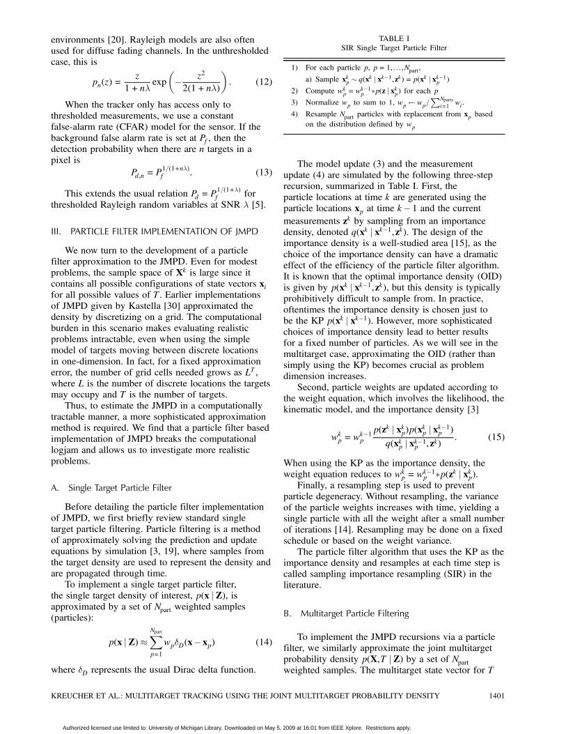
TABLE ISIR Single Target Particle Filter

1) For each particle p, p= 1, : : : ,Npart,

a) Sample xkp » q(xk j xk¡1,zk) = p(xk j xk¡1p )

2) Compute wkp = wk¡1p ¤p(z j xkp) for each p

3) Normalize wp to sum to 1, wpÃ wp=PNparts

i=1 wi.

4) Resample Npart particles with replacement from xp basedon the distribution defined by wp

The model update (3) and the measurementupdate (4) are simulated by the following three-steprecursion, summarized in Table I. First, theparticle locations at time k are generated using theparticle locations xp at time k¡ 1 and the currentmeasurements zk by sampling from an importancedensity, denoted q(xk j xk¡1,zk). The design of theimportance density is a well-studied area [15], as thechoice of the importance density can have a dramaticeffect of the efficiency of the particle filter algorithm.It is known that the optimal importance density (OID)is given by p(xk j xk¡1,zk), but this density is typicallyprohibitively difficult to sample from. In practice,oftentimes the importance density is chosen just tobe the KP p(xk j xk¡1). However, more sophisticatedchoices of importance density lead to better resultsfor a fixed number of particles. As we will see in themultitarget case, approximating the OID (rather thansimply using the KP) becomes crucial as problemdimension increases.Second, particle weights are updated according to

the weight equation, which involves the likelihood, thekinematic model, and the importance density [3]

wkp = wk¡1p

p(zk j xkp)p(xkp j xk¡1p )

q(xkp j xk¡1p ,zk): (15)

When using the KP as the importance density, theweight equation reduces to wkp = w

k¡1p ¤p(zk j xkp).

Finally, a resampling step is used to preventparticle degeneracy. Without resampling, the varianceof the particle weights increases with time, yielding asingle particle with all the weight after a small numberof iterations [14]. Resampling may be done on a fixedschedule or based on the weight variance.The particle filter algorithm that uses the KP as the

importance density and resamples at each time step iscalled sampling importance resampling (SIR) in theliterature.

B. Multitarget Particle Filtering

To implement the JMPD recursions via a particlefilter, we similarly approximate the joint multitargetprobability density p(X,T j Z) by a set of Npartweighted samples. The multitarget state vector for T



TABLE IISIR Multitarget Particle Filter

1) For each particle p, p= 1, : : : ,Npart,

a) For each partition t, t = 1, : : : ,Tp,

i) Sample Xkp,t » q(Xk ,Tk jXk¡1,Tk¡1,zk) =p(Xkp,t jXk¡1p,t )

2) Compute wkp = wk¡1p ¤p(z j Xp) for each p

3) Normalize wp to sum to 1, wpÃ wp=PNparts

i=1 wi.

4) Resample Npart particles with replacement from Xpbased on wp

targets is written as

X= [x1,x2, : : : ,xT¡1,xT]: (16)

The particle state vector for Tp targets is

Xp = [xp,1,xp,2, : : :xp,Tp] (17)

where Tp can be any nonnegative integer. We refer toxp,j as partition j of particle p. With ±D denoting theDirac delta, we define

±(X¡Xp) =½0 T 6= Tp±D(X¡Xp) otherwise

: (18)

Then the particle filter approximation to the JMPDis given by a set of particles Xp and correspondingweights wp as

p(X,T j Z)¼NpartXp=1

wp±(X¡Xp) (19)

wherePwp = 1.

Different particles in the approximation maycorrespond to different estimates of the number Tpof targets in the surveillance region. In practice, themaximum number of targets a particle may track istruncated at some large finite number Tmax.The JMPD p(X,T j Z) is defined for all possible

numbers of targets, T = 0,1,2, : : :. As each of theparticles Xp, p= 1 : : :Npart is a sample drawn from theJMPD p(X,T j Z), a particle Xp may have 0,1,2, : : :partitions, each partition corresponding to a differenttarget. Note that it is possible to have two or moretargets in the same state. We have denoted the numberof partitions in the pth particle Xp by Tp, where Tpmay be different for different Xp. Since a partitioncorresponds to a target, the number of partitions that aparticle has is that particle’s estimate of the number oftargets in the surveillance area.With these definitions the SIR particle filter

extends directly to JMPD filtering, as shown inTable II. This simply proposes new particles at timek using the particles at time k¡ 1 and the targetkinematics model (5) while (11) is used in the weightupdate.Again, since the model of target kinematics

p(Xk jXk¡1) is used to propose particles, the weight

equation (15) simplifies to become the measurementlikelihood p(z jXp).Targets entering or leaving the surveillance region

can be accounted for by modifying the proposaldensity to incorporate a probability that the proposedparticle Xkp has either fewer targets or more targetsthen Xk¡1p . For example, assume a per target deathrate of ®, which may be spatially varying to accountfor the fact that targets exit along the boundaries ofthe surveillance region. Then when proposing newparticles, with probability ®, partitions are removedfrom proposed particle p and the updated number oftargets in this particle Tkp is correspondingly reducedfrom Tk¡1p . In Table II, step 1a is modified so thateach partition is proposed forward with probability1¡®, rather than with probability 1.Further, assume a birth rate ¯. Then when

proposing new particles, with probability ¯, a newtarget is added to particle p. The location of the newtarget may be random, or more realistically chosenalong the perimeter of the surveillance area. In thiscase, the number of targets represented by this particleis updated to Tkp = T

k¡1p +1. Again, this modifies step

1a in Table II, in that one extra partition is proposedto exist in particle p at time k with probability ¯. Thistarget birth/death model is similar to other models,e.g. see [43] and [58], that have been proposed formultiple target tracking.More complicated models of target birth and

death (e.g. multiple targets arriving simultaneously,or targets arriving when existing targets are in certainstrategically important places, etc.) are permissibleunder this framework but are not considered here.

C. Multitarget Particle Proposal

Using the KP as the importance density hasthe benefit that it is simple to implement and iscomputationally inexpensive on a per particle basis.As we will see later, this computational efficiency iserased by the fact that a very large number of particlesare required using this importance density. Oneobvious drawback is that the KP does not explicitlytake advantage of the fact that the state vector in factrepresents many targets. Targets that are far apart inmeasurement space behave independently and shouldbe treated as such. A second drawback, common tomany particle filtering applications, is that the currentmeasurements are not used when proposing newparticles. These two considerations taken togetherresult in an inefficient use of particles and thereforerequire large numbers of particles to successfullytrack.To overcome these deficiencies, we have employed

alternative particle proposal techniques which biasthe proposal process towards the measurementsand allow for factorization of the target state when



permissible. These strategies propose each partition(target) in a particle separately, and form new particlesas the combination of the proposed partitions. Wedescribe two methods here, the independent partitions(IP) method of [52] and the coupled partitions (CP)method. The basic idea of both CP and IP is toconstruct particle proposals at the partition level,incorporating the measurements so as to bias theproposal towards the optimal importance density.We show that each has benefits and drawbacksand propose an adaptive partition (AP) methodwhich automatically switches between the two asappropriate.The permutation symmetry of the JMPD must be

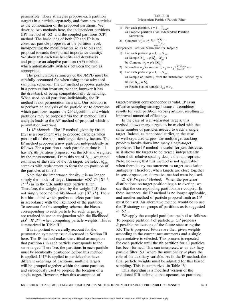
carefully accounted for when using these advancedsampling schemes. The CP method proposes particlesin a permutation invariant manner, however it hasthe drawback of being computationally demanding.When used on all partitions individually, the IPmethod is not permutation invariant. Our solution isto perform an analysis of the particle set to determinewhich partitions require the CP algorithm, and whichpartitions may be proposed via the IP method. Thisanalysis leads to the AP method of proposal which ispermutation invariant.1) IP Method: The IP method given by Orton

[52] is a convenient way to propose particles whenpart or all of the joint multitarget density factors. TheIP method proposes a new partition independently asfollows. For a partition t, each particle at time k¡ 1has it’s tth partition proposed via the KP and weightedby the measurements. From this set of Npart weightedestimates of the state of the tth target, we select Npartsamples with replacement to form the tth partition ofthe particles at time k.Note that the importance density q is no longer

simply the model of target kinematics p(Xk,Tk jXk¡1,Tk¡1) as in the SIR multitarget particle filter.Therefore, the weight given by the weight (15) doesnot simply become the likelihood p(zk jXk,Tk). Thereis a bias added which prefers to select partitionsin accordance with the likelihood of the partition.To account for this sampling scheme, the biasescorresponding to each particle for each target bp,tare retained to use in conjunction with the likelihoodp(zk jXk,Tk) when computing particle weights. This issummarized in Table III.It is important to carefully account for the

permutation symmetry issue discussed in Section IIIhere. The IP method makes the critical assumptionthat partition t in each particle corresponds to thesame target. Therefore, the partitions in each particlemust be identically positioned before this methodis applied. If IP is applied to particles that havedifferent orderings of partitions, multiple targetswill be grouped together within the same partitionand erroneously used to propose the location of asingle target. However, when this assumption of

TABLE IIIIndependent Partition Particle Filter

1) For each partition, t = 1 ¢ ¢ ¢Tmax,a) Propose partition t via Independent PartitionSubroutine

2) Compute wkp = wk¡1p ¤ p(zjXp)QTp

t=1bp,t

Independent Partition Subroutine for Target t:

1) For each particle p= 1, : : : ,Npart,

a) Sample X¤p,t » p(Xkp,t j Xk¡1p,t )

b) Compute wp = p(z j X¤p,t)2) Normalize wp to sum to 1, wpÃ wp=

PNpartsi=1 wi.


a) Sample an index j from the distribution defined by w

b) Set Xp,t =X¤j,t

c) Retain bias of sample, bp,t = wj

target/partition correspondence is valid, IP is aneffective sampling strategy because it combinesresults for each partition across particles, resulting inimproved numerical efficiency.In the case of well-separated targets, this

method allows many targets to be tracked with thesame number of particles needed to track a singletarget. Indeed, as mentioned earlier, in the caseof well-separated targets, the multitarget trackingproblem breaks down into many single-targetproblems. The IP method is useful for just this case,as it allows the targets to be treated independentlywhen their relative spacing deems that appropriate.Note, however, that this method is not applicablewhen there is any measurement-to-target associationambiguity. Therefore, when targets are close togetherin sensor space, an alternative method must be used.2) CP Proposal Method: When the posterior

distributions on target position begin to overlap, wesay that the corresponding partitions are coupled. Inthese instances, the IP method is no longer applicable,and another method of particle proposal such as CPmust be used. An alternative method would be to usethe IP strategy on groups of partitions as is suggestedin [52].We apply the coupled partitions method as follows.

To propose partition t of particle p, CP proposesR possible realizations of the future state using theKP. The R proposed futures are then given weightsaccording to the current measurements and a singlerepresentative is selected. This process is repeatedfor each particle until the tth partition for all particleshas been formed. This can interpreted as an auxiliaryparticle filter [53] where the multiplicity R plays therole of the auxiliary variable. As in the IP method, thefinal particle weights must be adjusted for this biasedsampling. This is summarized in Table IV.This algorithm is a modified version of the

traditional SIR technique that operates on partitions



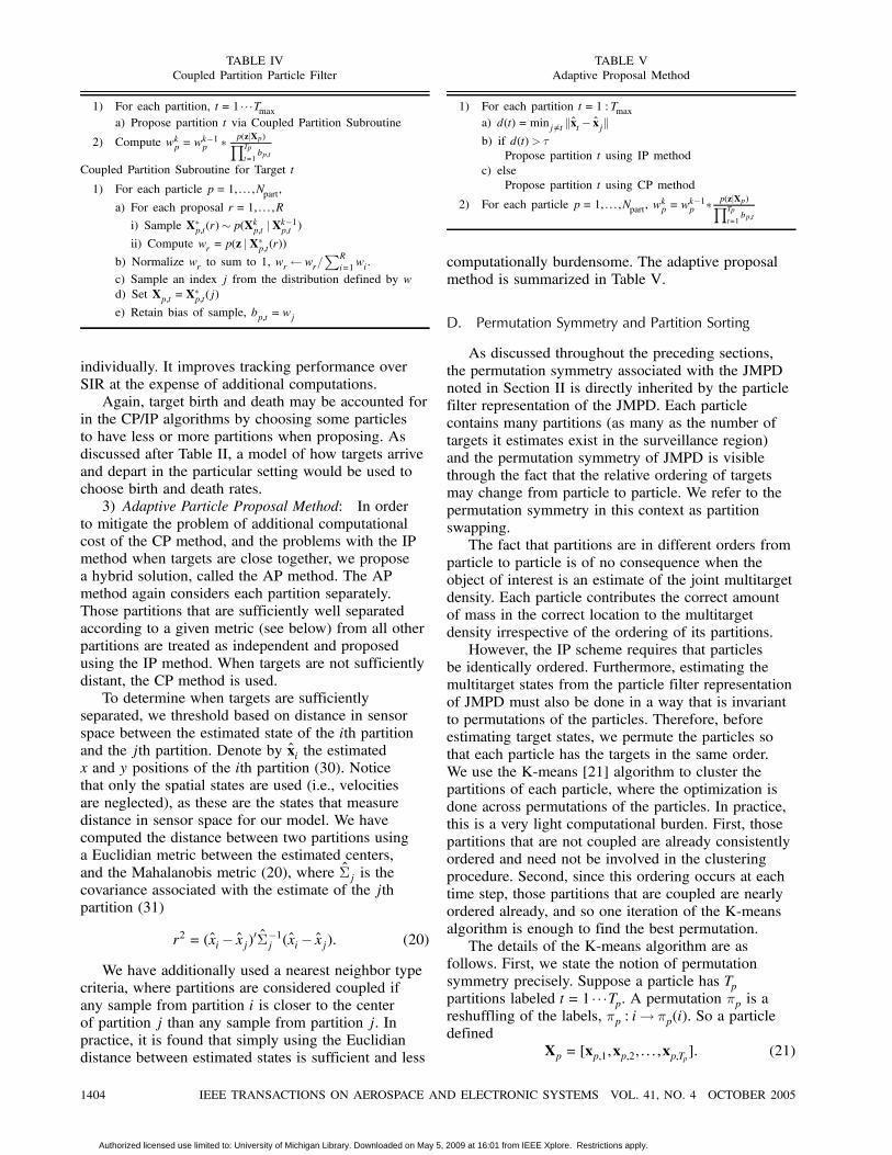
TABLE IVCoupled Partition Particle Filter

1) For each partition, t= 1 ¢ ¢ ¢Tmaxa) Propose partition t via Coupled Partition Subroutine

2) Compute wkp = wk¡1p ¤ p(zjXp)QTp

t=1bp,t

Coupled Partition Subroutine for Target t


a) For each proposal r = 1, : : : ,R

i) Sample X¤p,t(r)» p(Xkp,t j Xk¡1p,t )

ii) Compute wr = p(z j X¤p,t(r))b) Normalize wr to sum to 1, wrÃ wr=

PR

i=1wi.

c) Sample an index j from the distribution defined by wd) Set Xp,t =X

¤p,t(j)

e) Retain bias of sample, bp,t = wj

individually. It improves tracking performance overSIR at the expense of additional computations.Again, target birth and death may be accounted for

in the CP/IP algorithms by choosing some particlesto have less or more partitions when proposing. Asdiscussed after Table II, a model of how targets arriveand depart in the particular setting would be used tochoose birth and death rates.3) Adaptive Particle Proposal Method: In order

to mitigate the problem of additional computationalcost of the CP method, and the problems with the IPmethod when targets are close together, we proposea hybrid solution, called the AP method. The APmethod again considers each partition separately.Those partitions that are sufficiently well separatedaccording to a given metric (see below) from all otherpartitions are treated as independent and proposedusing the IP method. When targets are not sufficientlydistant, the CP method is used.To determine when targets are sufficiently

separated, we threshold based on distance in sensorspace between the estimated state of the ith partitionand the jth partition. Denote by xi the estimatedx and y positions of the ith partition (30). Noticethat only the spatial states are used (i.e., velocitiesare neglected), as these are the states that measuredistance in sensor space for our model. We havecomputed the distance between two partitions usinga Euclidian metric between the estimated centers,and the Mahalanobis metric (20), where §j is thecovariance associated with the estimate of the jthpartition (31)

r2 = (xi¡ xj)0§¡1j (xi¡ xj): (20)

We have additionally used a nearest neighbor typecriteria, where partitions are considered coupled ifany sample from partition i is closer to the centerof partition j than any sample from partition j. Inpractice, it is found that simply using the Euclidiandistance between estimated states is sufficient and less

TABLE VAdaptive Proposal Method

1) For each partition t= 1 : Tmaxa) d(t) = minj 6=t kxt ¡ xjkb) if d(t)> ¿

Propose partition t using IP methodc) else

Propose partition t using CP method

2) For each particle p= 1, : : : ,Npart, wkp = w

k¡1p ¤ p(zjXp)QTp

t=1bp,t

computationally burdensome. The adaptive proposalmethod is summarized in Table V.

D. Permutation Symmetry and Partition Sorting

As discussed throughout the preceding sections,the permutation symmetry associated with the JMPDnoted in Section II is directly inherited by the particlefilter representation of the JMPD. Each particlecontains many partitions (as many as the number oftargets it estimates exist in the surveillance region)and the permutation symmetry of JMPD is visiblethrough the fact that the relative ordering of targetsmay change from particle to particle. We refer to thepermutation symmetry in this context as partitionswapping.The fact that partitions are in different orders from

particle to particle is of no consequence when theobject of interest is an estimate of the joint multitargetdensity. Each particle contributes the correct amountof mass in the correct location to the multitargetdensity irrespective of the ordering of its partitions.However, the IP scheme requires that particles

be identically ordered. Furthermore, estimating themultitarget states from the particle filter representationof JMPD must also be done in a way that is invariantto permutations of the particles. Therefore, beforeestimating target states, we permute the particles sothat each particle has the targets in the same order.We use the K-means [21] algorithm to cluster thepartitions of each particle, where the optimization isdone across permutations of the particles. In practice,this is a very light computational burden. First, thosepartitions that are not coupled are already consistentlyordered and need not be involved in the clusteringprocedure. Second, since this ordering occurs at eachtime step, those partitions that are coupled are nearlyordered already, and so one iteration of the K-meansalgorithm is enough to find the best permutation.The details of the K-means algorithm are as

follows. First, we state the notion of permutationsymmetry precisely. Suppose a particle has Tppartitions labeled t= 1 ¢ ¢ ¢Tp. A permutation ¼p is areshuffling of the labels, ¼p : i! ¼p(i). So a particledefined

Xp = [xp,1,xp,2, : : : ,xp,Tp]: (21)



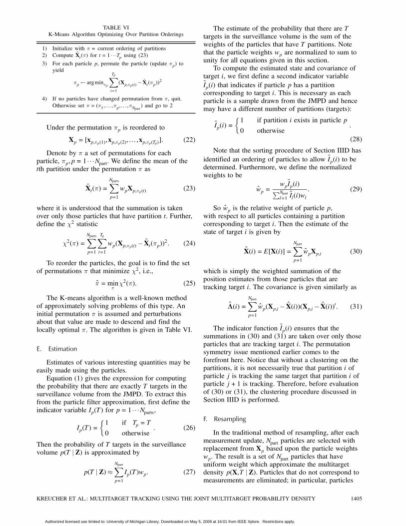
TABLE VIK-Means Algorithm Optimizing Over Partition Orderings

1) Initialize with ¼ = current ordering of partitions2) Compute Xt(¼) for t= 1 ¢ ¢ ¢Tp using (23)3) For each particle p, permute the particle (update ¼p) to

yield

¼pÃ argmin¼p

TpXt=1

(Xp,¼p(t) ¡ Xt(¼p))2

4) If no particles have changed permutation from ¼, quit.Otherwise set ¼ = (¼1, : : : ,¼p, : : : ,¼Npart ) and go to 2

Under the permutation ¼p is reordered to

Xp = [xp,¼p(1),xp,¼p(2), : : : ,xp,¼p(Tp)]: (22)

Denote by ¼ a set of permutations for eachparticle, ¼p,p= 1 ¢ ¢ ¢Npart. We define the mean of thetth partition under the permutation ¼ as

Xt(¼) =NpartsXp=1

wpXp,¼p(t) (23)

where it is understood that the summation is takenover only those particles that have partition t. Further,define the Â2 statistic

Â2(¼) =NpartsXp=1

TpXt=1

wp(Xp,¼p(t)¡ Xt(¼p))2: (24)

To reorder the particles, the goal is to find the setof permutations ¼ that minimize Â2, i.e.,

¼ =min¼Â2(¼): (25)

The K-means algorithm is a well-known methodof approximately solving problems of this type. Aninitial permutation ¼ is assumed and perturbationsabout that value are made to descend and find thelocally optimal ¼. The algorithm is given in Table VI.

E. Estimation

Estimates of various interesting quantities may beeasily made using the particles.Equation (1) gives the expression for computing

the probability that there are exactly T targets in thesurveillance volume from the JMPD. To extract thisfrom the particle filter approximation, first define theindicator variable Ip(T) for p= 1 ¢ ¢ ¢Nparts,

Ip(T) =½1 if Tp = T

0 otherwise: (26)

Then the probability of T targets in the surveillancevolume p(T j Z) is approximated by

p(T j Z)¼NpartXp=1

Ip(T)wp: (27)

The estimate of the probability that there are Ttargets in the surveillance volume is the sum of theweights of the particles that have T partitions. Notethat the particle weights wp are normalized to sum tounity for all equations given in this section.To compute the estimated state and covariance of

target i, we first define a second indicator variableIp(i) that indicates if particle p has a partitioncorresponding to target i. This is necessary as eachparticle is a sample drawn from the JMPD and hencemay have a different number of partitions (targets):

Ip(i) =½1 if partition i exists in particle p

0 otherwise:

(28)

Note that the sorting procedure of Section IIID hasidentified an ordering of particles to allow Ip(i) to bedetermined. Furthermore, we define the normalizedweights to be

wp =wpIp(i)PNpartl=1 Il(i)wl

: (29)

So wp is the relative weight of particle p,with respect to all particles containing a partitioncorresponding to target i. Then the estimate of thestate of target i is given by

X(i) = E[X(i)] =NpartXp=1

wpXp,i (30)

which is simply the weighted summation of theposition estimates from those particles that aretracking target i. The covariance is given similarly as

¤(i) =NpartXp=1

wp(Xp,i¡ X(i))(Xp,i¡ X(i))0: (31)

The indicator function Ip(i) ensures that thesummations in (30) and (31) are taken over only thoseparticles that are tracking target i. The permutationsymmetry issue mentioned earlier comes to theforefront here. Notice that without a clustering on thepartitions, it is not necessarily true that partition i ofparticle j is tracking the same target that partition i ofparticle j+1 is tracking. Therefore, before evaluationof (30) or (31), the clustering procedure discussed inSection IIID is performed.

F. Resampling

In the traditional method of resampling, after eachmeasurement update, Npart particles are selected withreplacement from Xp based upon the particle weightswp. The result is a set of Npart particles that haveuniform weight which approximate the multitargetdensity p(X,T j Z). Particles that do not correspond tomeasurements are eliminated; in particular, particles



whose Tp value is not supported by measurements(too many or too few targets) are selected with lowprobability.The particular resampling that was used in this

work is systematic resampling [3]. This resamplingstrategy is easily implemented, runs in order Nparts, isunbiased, and minimizes the Monte Carlo variance.Many other resampling schemes and modificationsare presented in the literature [15]. Of these methods,we have found that adaptively choosing at whichtime steps to resample [40] based on the number ofeffective particles leads to improved performancewhile reducing compute time. All results presentedherein use the method of [40] to determine whichtimes to resample and use systematic resampling[3] to perform resampling. We have also found thatMarkov chain Monte Carlo (McMC) moves usinga Metropolis-Hastings scheme [15] leads to slightlyimproved performance in our application.

IV. SIMULATION RESULTS

A. Introduction

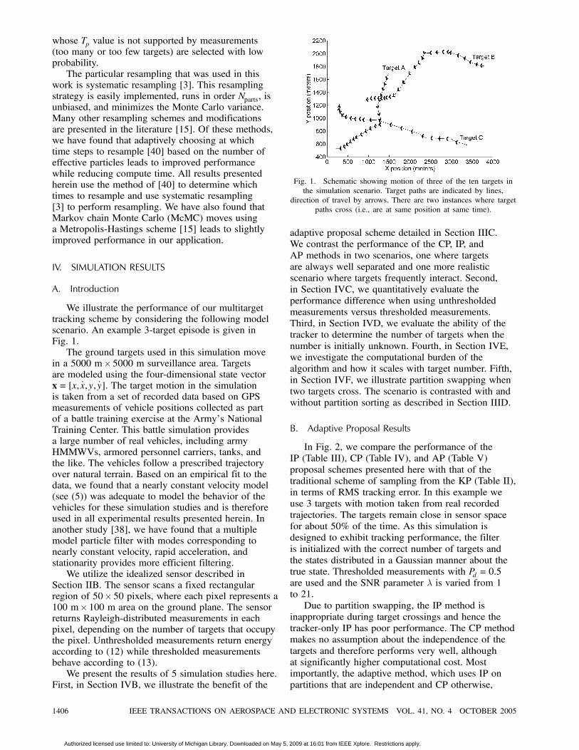
We illustrate the performance of our multitargettracking scheme by considering the following modelscenario. An example 3-target episode is given inFig. 1.The ground targets used in this simulation move

in a 5000 m£5000 m surveillance area. Targetsare modeled using the four-dimensional state vectorx= [x, _x,y, _y]. The target motion in the simulationis taken from a set of recorded data based on GPSmeasurements of vehicle positions collected as partof a battle training exercise at the Army’s NationalTraining Center. This battle simulation providesa large number of real vehicles, including armyHMMWVs, armored personnel carriers, tanks, andthe like. The vehicles follow a prescribed trajectoryover natural terrain. Based on an empirical fit to thedata, we found that a nearly constant velocity model(see (5)) was adequate to model the behavior of thevehicles for these simulation studies and is thereforeused in all experimental results presented herein. Inanother study [38], we have found that a multiplemodel particle filter with modes corresponding tonearly constant velocity, rapid acceleration, andstationarity provides more efficient filtering.We utilize the idealized sensor described in

Section IIB. The sensor scans a fixed rectangularregion of 50£ 50 pixels, where each pixel represents a100 m£ 100 m area on the ground plane. The sensorreturns Rayleigh-distributed measurements in eachpixel, depending on the number of targets that occupythe pixel. Unthresholded measurements return energyaccording to (12) while thresholded measurementsbehave according to (13).We present the results of 5 simulation studies here.

First, in Section IVB, we illustrate the benefit of the

Fig. 1. Schematic showing motion of three of the ten targets inthe simulation scenario. Target paths are indicated by lines,

direction of travel by arrows. There are two instances where targetpaths cross (i.e., are at same position at same time).

adaptive proposal scheme detailed in Section IIIC.We contrast the performance of the CP, IP, andAP methods in two scenarios, one where targetsare always well separated and one more realisticscenario where targets frequently interact. Second,in Section IVC, we quantitatively evaluate theperformance difference when using unthresholdedmeasurements versus thresholded measurements.Third, in Section IVD, we evaluate the ability of thetracker to determine the number of targets when thenumber is initially unknown. Fourth, in Section IVE,we investigate the computational burden of thealgorithm and how it scales with target number. Fifth,in Section IVF, we illustrate partition swapping whentwo targets cross. The scenario is contrasted with andwithout partition sorting as described in Section IIID.

B. Adaptive Proposal Results

In Fig. 2, we compare the performance of theIP (Table III), CP (Table IV), and AP (Table V)proposal schemes presented here with that of thetraditional scheme of sampling from the KP (Table II),in terms of RMS tracking error. In this example weuse 3 targets with motion taken from real recordedtrajectories. The targets remain close in sensor spacefor about 50% of the time. As this simulation isdesigned to exhibit tracking performance, the filteris initialized with the correct number of targets andthe states distributed in a Gaussian manner about thetrue state. Thresholded measurements with Pd = 0:5are used and the SNR parameter ¸ is varied from 1to 21.Due to partition swapping, the IP method is

inappropriate during target crossings and hence thetracker-only IP has poor performance. The CP methodmakes no assumption about the independence of thetargets and therefore performs very well, althoughat significantly higher computational cost. Mostimportantly, the adaptive method, which uses IP onpartitions that are independent and CP otherwise,



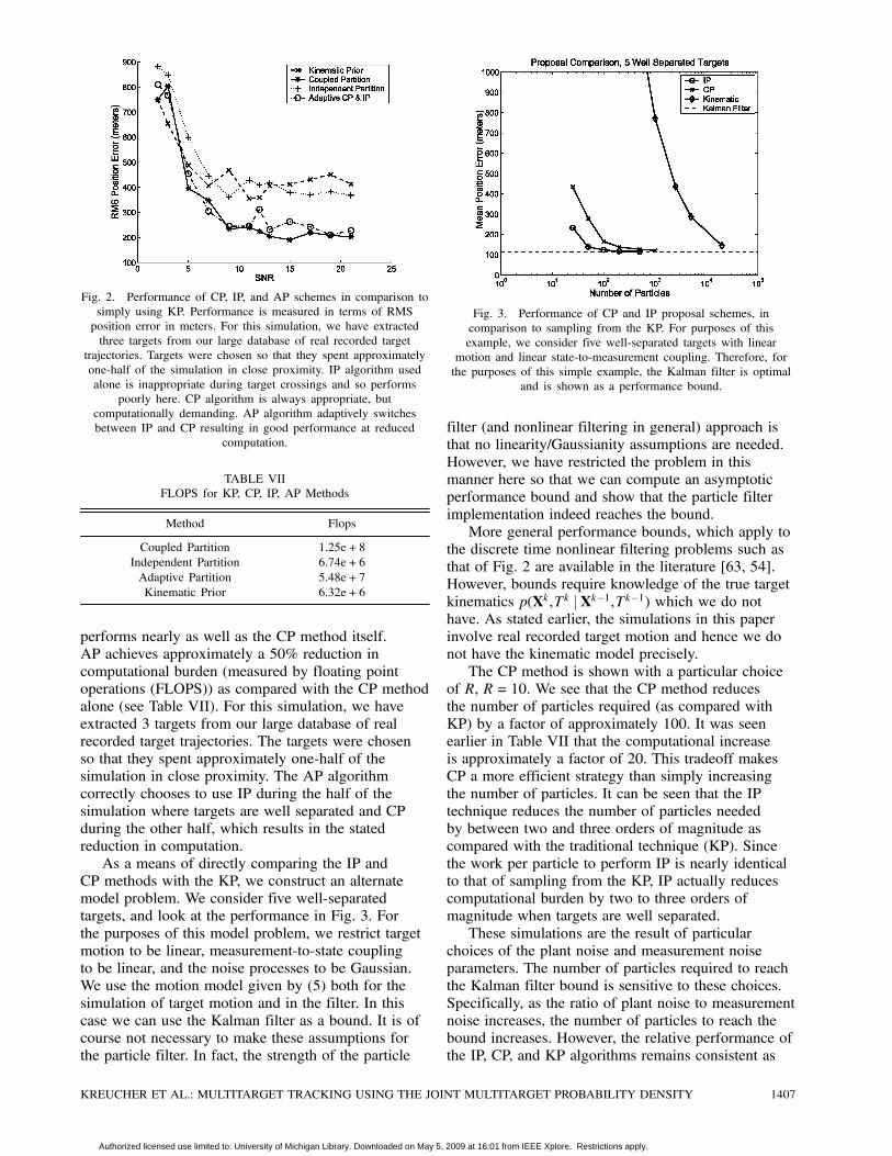
Fig. 2. Performance of CP, IP, and AP schemes in comparison tosimply using KP. Performance is measured in terms of RMSposition error in meters. For this simulation, we have extractedthree targets from our large database of real recorded target

trajectories. Targets were chosen so that they spent approximatelyone-half of the simulation in close proximity. IP algorithm usedalone is inappropriate during target crossings and so performs

poorly here. CP algorithm is always appropriate, butcomputationally demanding. AP algorithm adaptively switchesbetween IP and CP resulting in good performance at reduced

computation.

TABLE VIIFLOPS for KP, CP, IP, AP Methods

Method Flops

Coupled Partition 1:25e+8Independent Partition 6:74e+6Adaptive Partition 5:48e+7Kinematic Prior 6:32e+6

performs nearly as well as the CP method itself.AP achieves approximately a 50% reduction incomputational burden (measured by floating pointoperations (FLOPS)) as compared with the CP methodalone (see Table VII). For this simulation, we haveextracted 3 targets from our large database of realrecorded target trajectories. The targets were chosenso that they spent approximately one-half of thesimulation in close proximity. The AP algorithmcorrectly chooses to use IP during the half of thesimulation where targets are well separated and CPduring the other half, which results in the statedreduction in computation.As a means of directly comparing the IP and

CP methods with the KP, we construct an alternatemodel problem. We consider five well-separatedtargets, and look at the performance in Fig. 3. Forthe purposes of this model problem, we restrict targetmotion to be linear, measurement-to-state couplingto be linear, and the noise processes to be Gaussian.We use the motion model given by (5) both for thesimulation of target motion and in the filter. In thiscase we can use the Kalman filter as a bound. It is ofcourse not necessary to make these assumptions forthe particle filter. In fact, the strength of the particle

Fig. 3. Performance of CP and IP proposal schemes, incomparison to sampling from the KP. For purposes of thisexample, we consider five well-separated targets with linear

motion and linear state-to-measurement coupling. Therefore, forthe purposes of this simple example, the Kalman filter is optimal

and is shown as a performance bound.

filter (and nonlinear filtering in general) approach isthat no linearity/Gaussianity assumptions are needed.However, we have restricted the problem in thismanner here so that we can compute an asymptoticperformance bound and show that the particle filterimplementation indeed reaches the bound.More general performance bounds, which apply to

the discrete time nonlinear filtering problems such asthat of Fig. 2 are available in the literature [63, 54].However, bounds require knowledge of the true targetkinematics p(Xk,Tk jXk¡1,Tk¡1) which we do nothave. As stated earlier, the simulations in this paperinvolve real recorded target motion and hence we donot have the kinematic model precisely.The CP method is shown with a particular choice

of R, R = 10. We see that the CP method reducesthe number of particles required (as compared withKP) by a factor of approximately 100. It was seenearlier in Table VII that the computational increaseis approximately a factor of 20. This tradeoff makesCP a more efficient strategy than simply increasingthe number of particles. It can be seen that the IPtechnique reduces the number of particles neededby between two and three orders of magnitude ascompared with the traditional technique (KP). Sincethe work per particle to perform IP is nearly identicalto that of sampling from the KP, IP actually reducescomputational burden by two to three orders ofmagnitude when targets are well separated.These simulations are the result of particular

choices of the plant noise and measurement noiseparameters. The number of particles required to reachthe Kalman filter bound is sensitive to these choices.Specifically, as the ratio of plant noise to measurementnoise increases, the number of particles to reach thebound increases. However, the relative performance ofthe IP, CP, and KP algorithms remains consistent as



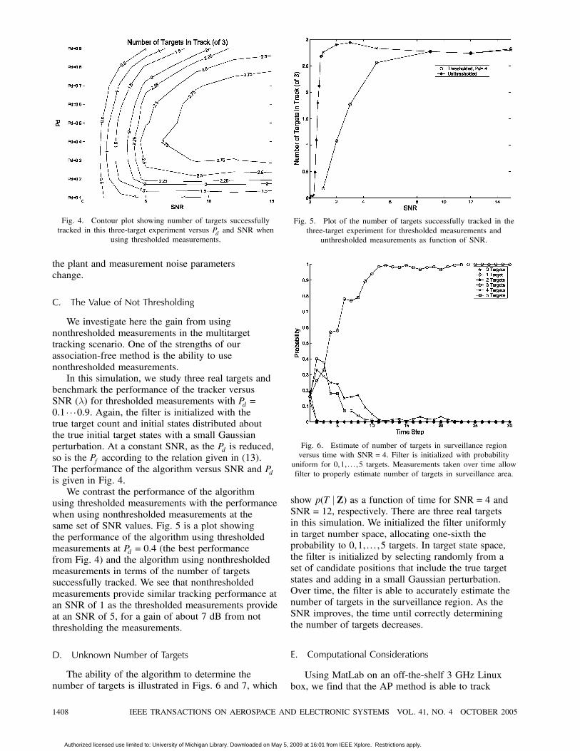
Fig. 4. Contour plot showing number of targets successfullytracked in this three-target experiment versus Pd and SNR when

using thresholded measurements.

the plant and measurement noise parameterschange.

C. The Value of Not Thresholding

We investigate here the gain from usingnonthresholded measurements in the multitargettracking scenario. One of the strengths of ourassociation-free method is the ability to usenonthresholded measurements.In this simulation, we study three real targets and

benchmark the performance of the tracker versusSNR (¸) for thresholded measurements with Pd =0:1 ¢ ¢ ¢0:9. Again, the filter is initialized with thetrue target count and initial states distributed aboutthe true initial target states with a small Gaussianperturbation. At a constant SNR, as the Pd is reduced,so is the Pf according to the relation given in (13).The performance of the algorithm versus SNR and Pdis given in Fig. 4.We contrast the performance of the algorithm

using thresholded measurements with the performancewhen using nonthresholded measurements at thesame set of SNR values. Fig. 5 is a plot showingthe performance of the algorithm using thresholdedmeasurements at Pd = 0:4 (the best performancefrom Fig. 4) and the algorithm using nonthresholdedmeasurements in terms of the number of targetssuccessfully tracked. We see that nonthresholdedmeasurements provide similar tracking performance atan SNR of 1 as the thresholded measurements provideat an SNR of 5, for a gain of about 7 dB from notthresholding the measurements.

D. Unknown Number of Targets

The ability of the algorithm to determine thenumber of targets is illustrated in Figs. 6 and 7, which

Fig. 5. Plot of the number of targets successfully tracked in thethree-target experiment for thresholded measurements and

unthresholded measurements as function of SNR.

Fig. 6. Estimate of number of targets in surveillance regionversus time with SNR= 4. Filter is initialized with probability

uniform for 0,1, : : : ,5 targets. Measurements taken over time allowfilter to properly estimate number of targets in surveillance area.

show p(T j Z) as a function of time for SNR= 4 andSNR= 12, respectively. There are three real targetsin this simulation. We initialized the filter uniformlyin target number space, allocating one-sixth theprobability to 0,1, : : : ,5 targets. In target state space,the filter is initialized by selecting randomly from aset of candidate positions that include the true targetstates and adding in a small Gaussian perturbation.Over time, the filter is able to accurately estimate thenumber of targets in the surveillance region. As theSNR improves, the time until correctly determiningthe number of targets decreases.

E. Computational Considerations

Using MatLab on an off-the-shelf 3 GHz Linuxbox, we find that the AP method is able to track



Fig. 7. Estimate of number of targets in surveillance regionversus time with SNR= 12. Filter is initialized with probabilityuniform for 0,1, : : : ,5 targets. Measurements taken over time allowfilter to properly estimate number of targets in surveillance area.

Fig. 8. Performance of particle filter implementation of JMPDwhen tracking ten real targets. This set of targets contains twoconvoys (targets following each other closely throughout the

simulation), one of four targets and one of three targets. For eachsimulation, at each time step tracking error is measured as meantrack error for the ten targets. Plot shows median tracking erroracross all 50 simulations. Filter is initialized with true targetlocations and so initial tracking error is 0. Steady state trackingerror is on the order of 40 m. As mentioned earlier, the sensormeasures 100 m£ 100 m resolution cells on the ground. Particlefilter implementation of JMPD uses 250 particles which allows

near real time tracking.

10 real targets with scans of the surveillance areacoming in once per second in near real time (fortypical situations, the algorithm takes approximately1.5 s to process each 1 s of data). A more low-levelimplementation is anticipated to easily allow realtime tracking. Fig. 8 shows the tracking performancewhen using the particle filter implementation of JMPDon ten real targets. The plot is averaged of 50 trials,where in each trial a random set of 10 targets ischosen from our large database of real targets.

Fig. 9. FLOPS (as measured by MatLab) versus number oftargets. One factor that effects computations required is number ofclosely spaced targets, as coupling must be modeled explicitly andCP algorithm becomes necessary. We include for reference herethe average number of coupled targets over all simulations.

One factor that effects computation is the numberof coupled targets. This effect can have a greaterimpact on computational complexity then the numberof targets. When targets move close together, theircoupling must be explicitly modeled and the CPalgorithm becomes necessary. This algorithm issignificantly more computationally demanding thenthe IP method.In Fig. 9, we show the timing results of

simulations where 1 ¢ ¢ ¢10 targets are tracked. Weinclude for reference the average number of coupledtargets during the simulations. For each trial, weselect t targets at random from our collection ofreal recorded data. Depending on which targets areselected, they may or may not be coupled, resulting ina different level computational complexity. The plot inFig. 9 is averaged over 50 trials.

F. Partition Swapping

We illustrate in this section the issue of partitionswapping as discussed in Section IIID. When targetsare close together, measurement-to-target ambiguitymay result in partitions of individual particles beingreordered. In Fig. 10, we give a 9 time-step vignettewhich includes a target crossing. Initially, the targetsare well separated and identically ordered (e.g.Time = 44) and the IP method is used for particleproposal. When the targets cross (Time = 60),partition swapping occurs and the CP method mustbe used. Without partition sorting using the K-meansalgorithm of Section IIID, this swapping persists evenafter the targets separated and the CP method must beused even at Time = 84. This results in an inefficientalgorithm, as the CP method is more computationallydemanding.



Fig. 10. This figure illustrates the phenomenon of partition swapping that occurs in direct particle filter implementation of SIR filterfor JMPD. True target locations are indicated by a solid circle. At time 30 only one target is visible in plot window. At 44 s, both

targets can be seen and the two partitions for each particle, plotted with x and o, are well separated. From time 60 to 66, they occupythe same detection cell. At time 84, some partition swapping has occurred, indicated by the fact that there are mixtures of x and o

corresponding to each target location.

Fig. 11. This figure illustrates the same multitarget tracking scenario as in Fig. 10, except here we perform partition sorting at eachtime step. True target locations are indicated by a solid circle. At time 30 only one target is visible in plot window. At 44 s, both

targets can be seen and the two partitions for each particle, plotted with x and o, are well separated. From time 60 to 66, they occupythe same detection cell. Targets move apart starting at time 72. Notice that the partition swapping visible in Fig. 10 at times 72—84 is

avoided here because of partition sorting.

In Fig. 11 we show the same vignette as inFig. 10, but this time we use the partition sortingalgorithm outlined in Section IIID at each time step.While the CP method must still be used when thetargets are occupying the same detection cell, whenthey move out (Time= 72) the IP method may beused again. The partition sorting allows for the more

computationally efficient IP method to be used forproposal by reordering the particles appropriately.

V. CONCLUSION

This paper has presented a new grid-freeimplementation of a Bayesian method for tracking



multiple targets based on recursively estimatingthe JMPD. We have detailed an adaptive particleproposal scheme that explicitly takes into account themultitarget nature of the problem and automaticallyfactors it into a series of smaller independentproblems when appropriate, while properly treatingthe permutation symmetry and correlations that arisewhen targets are close together. This implementationreduces the computational burden to a reasonable leveland allows implementation for realistic problems. Insimulations with real target motion, we have shownthe ability to track ten targets with complicatedkinematic behavior, using pixelated measurements ona grid. This technique has the benefit that raw sensormeasurements may be directly incorporated throughthe use of a likelihood function. This algorithm canprocess unthresholded data, obtaining a 3—6 dBeffective gain compared with thresholded data.Furthermore, no measurement-to-target associationis explicitly required.

REFERENCES

[1] Alspach, D. L., and Sorensen, H. W.Nonlinear Bayesian estimation using Gaussian sumapproximations.IEEE Transactions on Automatic Control, 17, 4 (Aug.1972), 439—448.

[2] Arulampalam, M. S., and Ristic, B.Comparison of the particle filter with range arameterizedand modified polar EKFs for angle-only tracking.Proceedings of SPIE, 4048 (2000), 288—299.

[3] Arulampalam, M. S., Maskell, S., Gordon, N., and Clapp, T.A tutorial on particle filters for onlinenonlinear/non-Gaussian Bayesian tracking.IEEE Transactions on Signal Processing, 50, 2 (Feb.2002), 174—188.

[4] Bar-Shalom, Y., and Li, X. R.Estimation and Tracking: Principles, Techniques, andSoftware.Norwood, MA: Artech House, 1993.

[5] Bar-Shalom, Y.Multitarget Multisensor Tracking: Advanced Applications.Norwood, MA: Artech House, 1990.

[6] Bar-Shalom, Y., and Blair, W. D.Multitarget-Multisensor Tracking: Applications andAdvances, Vol. III.Norwood, MA: Artech House, 2000.

[7] Bergman, N.Recursive Bayesian estimation: Navigation and trackingapplications.Ph.D. dissertation, Linkoping University, Linkoping,Sweden, 1999.

[8] Blackman, S. S.Mulitple-Target Tracking with Radar Applications.Norwood, MA: Artech House, 1986.

[9] Blair, W. D., and Brandt-Pearce, M.Unresolved Rayleigh target detection using monopulsemeasurements.IEEE Transactions on Aerospace and Electronic Systems,34, 2 (1998), 543—552.

[10] Blom, H. A. P., and Bloem, E. A.Joint IMMPDA particle filter.In Proceedings of the 6th International Conference onInformation Fusion, Cairns, Queensland, Australia, July2003.

[11] Chood, K., and Fleet, D. J.People tracking using hybrid Monte Carlo filtering.In Proceedings of The International Conference onComputer Vision, vol. 2, 2001, 321—328.

[12] Crisan, D., and Doucet, A.A survey of convergence results on particle filteringmethods for practicioners.IEEE Transactions on Signal Processing, 50, 3 (2002),736—746.

[13] Dellaert, F., Fox, D., Burgard, W., and Thrun, S.Monte Carlo localization for mobile robots.Presented at IEEE International Conference on Roboticsand Automation, May 1999.

[14] Doucet, A.On sequential Monte Carlo methods for Bayesianfiltering.Technical report, Department of Engineering, Universityof Cambridge, UK, 1998.

[15] Doucet, A., de Freitas, N., and Gordon, N.Sequential Monte Carlo Methods in Practice.New York: Springer, 2001.

[16] Doucet, A., Vo, B-N., Andrieu, C., and Davy, M.Particle filtering for multi-target tracking and sensormanagement.Presented at The Fifth International Conference onInformation Fusion, Maryland, 2002.

[17] Gonzalez-Banos, H. H., Lee, C-Y., and Latombe, J-C.Real-time combinatorial tracking of a target movingunpredictably among obstacles.In Proceedings of the IEEE Conference on Robotics andAutomation, Washington, D.C., May 2002.

[18] Goodman, I., Mahler, R., and Nguyen, H.Mathematics of Data Fusion.Boston: Kluwer Academic Publishers, 1997.

[19] Gordon, N. J., Salmond, D. J., and Smith, A. F. M.A novel approach to non-linear and non-GaussianBayesian state estimation.IEE Proceedings on Radar and Signal Processing, 140(1993), 107—113.

[20] Gowda, C. H., and Viswanatha, R.Performance of distributed CFAR test under variousclutter amplitudes.IEEE Transactions on Aerospace and Electronic Systems,35, 4 (1999), 1410—1419.

[21] Hastie, T., Tibshirani, R., and Friedman, J.The Elements of Statistical Learning (Springer Series inStatistics).New York: Springer-Verlag, 2001.

[22] Hue, C., Le Cadre, J-P., and Perez, P.Tracking multiple objects with particle filtering.IEEE Transactions on Aerospace and Electronic Systems,38, 3 (2002), 791—812.

[23] Hue, C., Le Cadre, J-P., and Perez, P.Sequential Monte Carlo methods for multiple targettracking and data fusion.IEEE Transactions on Signal Processing, 50, 2 (2002),309—325.

[24] Isard, M., and Blake, A.Visual tracking by stochastic propagation of conditionaldensity.In Proceedings of the 4th European Conference onComputer Vision, Cambridge, England, 1996, 343—356.

[25] Isard, M., and MacCormick, J.BraMBLe: A Bayesian multiple-blob tracker.In Proceedings of the 8th International Conference onComputer Vision, 2001.



[26] Jazwinski, A. H.Stochastic Processes and Filtering Theory.New York: Academic Press, 1970.

[27] Julier, S. J., and Uhlman, J. K.A new extension of the Kalman filter to nonlinearsystems.In Proceedings of Aerosense: The Eleventh InternationalSymposium on Aerospace/Defense Sensing, Simulation andControls, vol. 3068, 1997, 182—193.

[28] Kamen, E. W.Multiple target tracking based on symmetric measurementfunctionsIEEE Transactions on Automatic Control, 37, 3 (1992),371—374.

[29] Karlsson, R., and Gustafsson, F.Monte Carlo data association for multiple target tracking.In Proceedings of the IEE Workshop on Target Tracking:Algorithms and Applications, The Netherlands, 2001.

[30] Kastella, K.Discrimination gain for sensor management in multitargetdetection and tracking.In IEEE-SMC and IMACS Multiconference CESA ’96, vol.1, Lille, France, July 9—12, 1996, 167—172.

[31] Kastella, K.A maximum likelihood estimator for report-to-trackassociation.SPIE Proceedings, 1954 (1993), 386—393.

[32] Kastella, K.Event-averaged maximum liklihood estimation andmean-field theory in multitarget tracking.IEEE Transactions on Automatic Control, 40, 6 (1995),1070—1074.

[33] Kastella, K.Event averaged maximum likelihood estimation andmean-field theory in multitarget tracking.IEEE Transactions on Automatic Control, 50, 6 (June1995), 1070—1073.

[34] Kirubarajan, T., and Bar-Shalom, Y.Probabilistic data association techniques for targettracking in clutter.Proceedings of the IEEE, 92, 3 (Mar. 2004), 536—557.

[35] Kitagawa, G.Non-Gaussian state-space modelling of non-stationarytime series.Journal of the American Statistical Association, 82 (1987),1032—1063.

[36] Kreucher, C., Kastella, K., and Hero, A. O.Tracking multiple targets using a particle filterrepresentation of the joint multitarget probability density.Presented at the SPIE International Symposium onOptical Science and Technology, San Diego, CA, Aug.2003.

[37] Kreucher, C., and Kastella, K.Multiple-model nonlinear filtering for low-signal groundtarget applications.In Proceedings of The Fifteenth International AerosenseSymposium, vol. 4380, 2001, 1—12.

[38] Kreucher, C., Hero, A. O., and Kastella, K.Multiple model particle filtering for multi-target tracking.In Proceedings of the Twelfth Annual Workshop onAdaptive Sensor Array Processing, Mar. 2004.

[39] Lee, M-S., and Kim, Y-H.An efficient multitarget tracking algorithm for carapplications.IEEE Transactions on Industrial Electronics, 50, 2 (2003),397—399.

[40] Liu, J., and Chen, R.Sequential Monte Carlo methods for dynamic systems.Journal of the American Statistical Association, (Sept.1998).

[41] Mahler, R. P. S.A unified foundation for data fusion.In The Seventh Joint Service Data Fusion Symposium,Laurel, MD, Oct. 25—28, 1994, 154—174.

[42] Mahler, R.Global optimal sensor allocation.In Proceedings of the Ninth National Symposium on SensorFusion, vol. I, Mar. 12—14, 1996, 167—172.

[43] Mahler, R.An extended first-order Bayes filter for force aggregation.In Proceedings of SPIE Conference on Signal and DataProcessing of Small Targets, vol. 4729, 2002.

[44] Mallick, M.Comparison of EKF, UKF, and PF for UGS and GMTIsensors.Presneted at The 2003 Defense Science and TechnologyWorkshop, Adelaide, Australia, July 2003.

[45] Maskell, S., Rollason, M., Gordon, N., and Salmond, D.Efficient particle filtering for multiple target tracking withapplication to tracking in structured images.In Proceedings of SPIE Conference on Signal and DataProcessing of Small Targets, 2002, Orlando, FL, Apr. 1—5,2002.

[46] Maybeck, P. S.Stochastic Models, Estimation, and Control, Vol. 1.New York: Academic Press, 1982.

[47] Mori, S., Shong, C. Y., Tse, E., and Wishner, R. P.Tracking and classifying multiple targets without a prioridentification.IEEE Transactions on Automatic Control, AC-31 (May1986).

[48] Miller, M. I., Srivastava, A., and Grenander, U.Conditional mean estimation via jump-diffusion processesin multiple target tracking/recognition.IEEE Transactions on Signal Processing, 43, 11 (1995),2678—2690.

[49] Musick, S., Kastella, K., and Mahler, R.A practical implementation of joint multitargetprobabilities.SPIE Proceedings, 3374 (1998), 26—37.

[50] Montemerlo, M., Thrun, S., and Whittaker, W.Conditional particle filter for simultaneous mobile robotlocalization and people tracking.In Procceedings of the IEEE Conference on Robotics andAutomation, vol. 1, 2002, 695—701.

[51] Musick, S., Greenewald, J., Kreucher, C., and Kastella, K.Comparison of particle method and finite differencenonlinear filters for low SNR target tracking.In Proceedings of The Fourth Annual Conference onInformation Fusion, Montreal, Canada, 2001.

[52] Orton, M., and Fitzgerald, W.A Bayesian approach to tracking multiple targets usingsensor arrays and particle filters.IEEE Transactions on Signal Processing, 50, 2 (2002),216—223.

[53] Pitt, M. K., and Shephard, N.Filtering via simulation: Auxiliary particle filters.Journal of the American Statistical Association, 94 (June1999), 446, 590—599.

[54] Ristic, B., and Arulampalam, M. S.Tracking a manoeuvring target using angle-onlymeasurements: Algorithms and performance.Signal Processing, 83 (2003), 1223—1238.



[55] Schulz, D., Fox, D., and Hightower, J.People tracking with anonymous and ID-sensors usingRao-Blackwellised particle filter.In Proceedings of the Eighteenth International JointConference on Artificial Intelligence, 2003.

[56] Shertukde, H. M., and Bar-Shalom, Y.Tracking of crossing targets with imaging sensors.IEEE Transactions on Aerospace and Electronic Systems,27, 4 (1991), 582—592.

[57] Sidenbladh, H., and Wirkander, S-L.Particle filtering for random sets.IEEE Transactions on Aerospace and Electronic Systems, tobe published.

[58] Sidenbladh, H., and Wirkander, S-L.Tracking random sets of vehicles in terrain.Presented at the IEEE Workshop on Multi-ObjectTracking, Madison, WI, 2003.

[59] (Special issue on particle filtering methods).IEEE Transactions on Signal Processing, 50, 2 (2002).

[60] Stimson, G. W.Introduction to Airborne Radar (2nd ed.).Rayleigh, NC: SciTech Publishing, 1998.

[61] Stone, L. D., Barlow, C. A., and Corwin, T. L.Bayesian Multiple Target Tracking.Norwood, MA: Artech House, 1999.

[62] Streit, R. L., and Luginbuhl, T. E.Maximum likelihood methods for probabilisticmulti-hypothesis tracking.Proceedings of SPIE, 2235 (Apr. 5—7, 1994).

[63] Tichavsky, P., Muravchik, C., and Nehorai, A.Posterior Cramer-Rao bounds for discrete-time nonlinearfiltering.IEEE Transactions on Signal Processing, 46, 5 (May1998), 1386—1396.

[64] Tullsson, B. E.Monopulse tracking of Rayleigh targets: A simpleapproach.IEEE Transactions on Aerospace and Electronic Systems,27, 3 (1991), 520—531.

[65] Tweed D., and Calway, A.Tracking multiple animals in wildlife footage.In Proceedings of the Conference on Pattern Recognition,vol. 2, 2002, 24—27.

[66] Vermaak, J., and Blake, A.Nonlinear filtering for speaker tracking in noisy andreverberant environments.In Proceedings of International Conference on AcousticsSpeech and Signal Processing, vol. V, 2001, 3021—3024.

[67] Vo, B-N., Singh, S., and Doucet, A.Sequential Monte Carlo implementatoin of the PHD filterfor multi-target tracking.In Proceedings of the Sixth International Conference onInformation Fusion, July 2993, 792—799.



Chris Kreucher received the B.S. and M.S. degrees from the University ofMichigan—Dearborn (1997 and 1998, respectively) and the Ph.D. degree from theUniversity of Michigan—Ann Arbor, in 2005, all in electrical engineering.Since 1997, he has been a research scientist at General Dynamics Advanced

Information Systems’ Michigan Research & Development Facility (formerlyknown as ERIM). His current research interests include Bayesian filtering(specifically multitarget tracking) and sensor management.

Keith Kastella received a B.A. in physics in 1980 from Reed College, PortlandOR, and the M.S. and Ph.D. degrees from the State University of New York atStony Brook (SUNY-SB) in 1985 and 1988, respectively.He is a chief scientist at General Dynamics Advanced Information Systems in

Ypsilanti, MI. His current research interests are in data fusion, signal processingand novel applications of quantum entanglement in sensing and signal processing.

Alfred O. Hero, III (S’79–M’80–SM’96–F’98) received the B.S. (summacum laude) from Boston University (1980) and the Ph.D from PrincetonUniversity (1984), both in electrical engineering.Since 1984 he has been with the University of Michigan, Ann Arbor, where

he is a professor in the Department of Electrical Engineering and ComputerScience, and by courtesy, in the Department of Biomedical Engineering andthe Department of Statistics. His recent research interests have been in areasincluding: inference on sensor networks, bioinformatics, and statistical signal andimage processing.Dr. Hero has received an IEEE Signal Processing Society Meritorious Service

Award (1998), an IEEE Signal Processing Society Best Paper Award (1998), andthe IEEE Third Millenium Medal (2000). He is currently president-elect of theIEEE Signal Processing Society (2004—2005) and associate editor of the IEEETransactions on Computational Biology and Bioinformatics (2004—2006).



multitarget tracking using the joint multitarget...

Documents