multistep methods - richard palais' home...

Appendix I

Multistep Methods

In this appendix, we provide a brief introduction to the derivation

of linear multistep methods and analyze the conditions on the coef-

ficients that are necessary and sufficient to guarantee convergence of

order 𝑃 .

Among the seven basic examples in Chapter 5, one was a two-step

method, the leapfrog method. Multistep methods potentially obtain

more accurate approximations from fewer costly evaluations of a vec-

tor field if prior evaluations and values of the solution are stored for

later use. With each additional stored value comes the need for an

additional value for initialization not provided by the analytical prob-

lem. Each of these carries an additional degree of potential instability

and adds to the cost of changing the step-size. In spite of this, some

multistep methods have desirable absolute stability properties. We

will also describe some relationships between the accuracy and sta-

bility of these methods.

Recall that we are considering methods for approximating solu-

tions of the IVP

y′ = f(𝑡,y), y(𝑡𝑜) = y𝑜, 𝑡 ∈ [𝑡𝑜, 𝑡𝑜 + 𝑇 ], y ∈ R𝐷, (I.1)

satisfying a Lipschitz condition in some norm on R𝐷,

∣∣f(𝑡,y1)− f(𝑡,y2)∣∣ ≤ 𝐿∣∣y1 − y2∣∣. (I.2)

For simplicity of exposition, we will henceforth use notation for the

scalar case, but unless otherwise noted, generalizations to the case

of systems are typically straightforward. In scalar notation, linear

281

282 I. Multistep Methods

𝑚-step methods take the form

𝑦𝑛+1 =𝑚−1∑𝑗=0

𝑎𝑗𝑦𝑛−𝑗 + ℎ𝑚−1∑𝑗=−1

𝑏𝑗𝑦′𝑛−𝑗 , (I.3)

for all integers 𝑛 satisfying 0 ≤ 𝑛ℎ ≤ 𝑇 . Here, 𝑡0 = 𝑡𝑜, 𝑡𝑛+1 = 𝑡𝑛 + ℎ,

𝑦′𝑗 = 𝑓(𝑡𝑗 , 𝑦𝑗), and 𝑦0, . . . , 𝑦𝑚−1 are initial values obtained by com-

panion methods discussed below. When the meaning is unambiguous,

we will leave the dependence of 𝑦𝑛 on ℎ implicit.

There are several strategies that may be used to obtain fami-

lies of linear 𝑚-step methods with higher-order accuracy. The first

such family we will consider is the 𝑚-step backward difference for-

mula methods, BDF𝑚. These methods are derived by replacing the

derivative on the left of 𝑦′(𝑡𝑛+1) = 𝑓(𝑡𝑛+1, 𝑦(𝑡𝑛+1)) with the approxi-

mation obtained by differentiating the polynomial 𝑝𝑚(𝑡) of degree 𝑚

that interpolates 𝑦(𝑡) at 𝑡𝑛+1, 𝑡𝑛, . . . , 𝑡𝑛+1−𝑚 and then discretizing.

For 𝑚 = 1, since

𝑝1(𝑡) = 𝑦(𝑡𝑛+1) + (𝑡− 𝑡𝑛+1)𝑦(𝑡𝑛+1)− 𝑦(𝑡𝑛)

ℎ,

we discretize

𝑦(𝑡𝑛+1)− 𝑦(𝑡𝑛)

ℎ= 𝑓(𝑡𝑛+1, 𝑦(𝑡𝑛+1))

and find that BDF1 is the Backward Euler Method,

𝑦𝑛+1 = 𝑦𝑛 + ℎ𝑓(𝑡𝑛+1, 𝑦𝑛+1).

For 𝑚 = 2, iterative interpolation, described in Appendix J, yields

𝑝2(𝑡) = 𝑦(𝑡𝑛+1) + (𝑡− 𝑡𝑛+1)[𝑦(𝑡𝑛+1)− 𝑦(𝑡𝑛)

ℎ

+ (𝑡− 𝑡𝑛)𝑦(𝑡𝑛+1)− 2𝑦(𝑡𝑛) + 𝑦(𝑡𝑛−1)

2ℎ2]

and

𝑝′2(𝑡𝑛+1) =3𝑦(𝑡𝑛+1)− 4𝑦(𝑡𝑛) + 𝑦(𝑡𝑛−1)

2ℎ.

Discretizing, we find that BDF2 is given by

𝑦𝑛+1 =4

3𝑦𝑛 − 1

3𝑦𝑛−1 +

2ℎ

3𝑓(𝑡𝑛+1, 𝑦𝑛+1).

I. Multistep Methods 283

The Adams family of methods arises when we approximate the

integral on the right of 𝑦(𝑡𝑛+1)− 𝑦(𝑡𝑛) =∫ 𝑡𝑛+1

𝑡𝑛𝑦′(𝑠) 𝑑𝑠 with

∫ 𝑡𝑛+1

𝑡𝑛

𝑃𝐴⋅𝑚 (𝑠) 𝑑𝑠.

where 𝑃𝐴⋅ interpolates 𝑦′(𝑠) at a prescribed set of time-steps, and

then discretize. For the explicit Adams-Bashforth Methods, AB𝑚,

𝑃𝐴𝐵𝑚 (𝑠) is the polynomial of degree 𝑚 that interpolates 𝑦′(𝑠) at

𝑡𝑛, . . . , 𝑡𝑛+1−𝑚. For the implicit Adams-Moulton Methods, AM𝑚,

𝑃𝐴𝑀𝑚 (𝑠) is the polynomial of degree 𝑚 + 1 that interpolates 𝑦′(𝑠) at

𝑡𝑛+1, 𝑡𝑛, . . . , 𝑡𝑛+1−𝑚.

For 𝑚 = 1, 𝑃𝐴𝐵1 (𝑠) = 𝑦′(𝑡𝑛), and we find that AB1 is Euler’s

Method. Moreover,

𝑃𝐴𝑀1 (𝑠) = 𝑦′(𝑡𝑛+1) + (𝑠− 𝑡𝑛+1)

𝑦′(𝑡𝑛+1)− 𝑦′(𝑡𝑛)ℎ

and ∫ 𝑡𝑛+1

𝑡𝑛

𝑃𝐴𝑀1 (𝑠) 𝑑𝑠 = ℎ

𝑦′(𝑡𝑛+1) + 𝑦′(𝑡𝑛)2

,

so we find that AM1 is the trapezoidal method. For 𝑚 = 2,

𝑃𝐴𝐵2 (𝑠) = 𝑦′(𝑡𝑛) + (𝑠− 𝑡𝑛)

𝑦′(𝑡𝑛)− 𝑦′(𝑡𝑛−1)

ℎ

and ∫ 𝑡𝑛+1

𝑡𝑛

𝑃𝐴𝐵2 (𝑠) 𝑑𝑠 = ℎ

3𝑦′(𝑡𝑛)− 𝑦′(𝑡𝑛−1)

2,

so AB2 is given by

𝑦𝑛+1 = 𝑦𝑛 + ℎ(3

2𝑦′𝑛 − 1

2𝑦′𝑛−1).

Again iterative interpolation yields

𝑃𝐴𝑀2 (𝑠) = 𝑦′(𝑡𝑛+1)+(𝑠− 𝑡𝑛+1)[

𝑦′(𝑡𝑛+1)− 𝑦′(𝑡𝑛)ℎ

+ (𝑠− 𝑡𝑛)𝑦′(𝑡𝑛+1)− 2𝑦′(𝑡𝑛) + 𝑦′(𝑡𝑛−1)

2ℎ2].

Using∫ 𝑡𝑛+1

𝑡𝑛

(𝑠− 𝑡𝑛+1)(𝑠− 𝑡𝑛) 𝑑𝑠 =

∫ ℎ

0

(𝑢2 − 𝑢ℎ) 𝑑𝑢 = −ℎ3/6


reduces this to∫ 𝑡𝑛+1

𝑡𝑛

𝑃𝐴𝑀2 (𝑠) 𝑑𝑠 = ℎ[

𝑦′(𝑡𝑛+1) + 𝑦′(𝑡𝑛)2

− 𝑦′(𝑡𝑛+1)− 2𝑦′(𝑡𝑛) + 𝑦′(𝑡𝑛−1)

12].

Discretizing, we find that AM2 is given by

𝑦𝑛+1 = 𝑦𝑛 + ℎ(5

12𝑦′𝑝 +

8

12𝑦′𝑛 − 1

12𝑦′𝑛−1).

Another strategy for deriving multistep methods obtains the co-

efficients 𝑎𝑗 , 𝑏𝑗 as solutions of linear equations that guarantee the

method is formally accurate of order 𝑃 . These conditions are related

to the order of accuracy of a convergent method by the local trunca-

tion error of the method, 𝜖𝑛. This quantity measures by how much

a solution of the differential equation fails to satisfy the difference

equation, in the sense

𝑦(𝑡𝑛+1) =𝑚−1∑𝑗=0

𝑎𝑗𝑦(𝑡𝑛−𝑗)

+ ℎ

𝑚−1∑𝑗=−1

𝑏𝑗𝑦′(𝑡𝑛−𝑗) + 𝜖𝑛, where 𝑦′𝑗 = 𝑓(𝑡𝑗 , 𝑦(𝑡𝑗)).

(I.4)

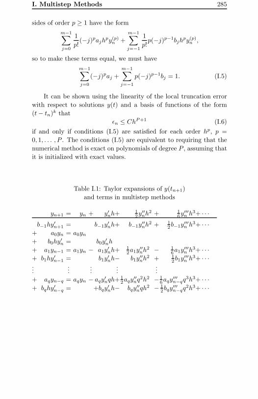
In its top row, Table I.1 contains the first few terms of the Taylor

expansion of the left-hand side of (I.4), 𝑦(𝑡𝑛+1), about 𝑡𝑛, in powers

of ℎ. Below the line, the rows contain the Taylor expansions of the

terms 𝑦(𝑡𝑛 − 𝑗ℎ) and 𝑦′(𝑡𝑛 − 𝑗ℎ) on the right of (I.4), where we have

placed terms of the same order in the same column and set 𝑞 = 𝑚 = 1

for compactness of notation.

Algebraic conditions that determine a bound on the order of 𝜖𝑛are obtained by comparing the collective expansions of both sides.

The terms in each column are multiples of ℎ𝑝𝑦(𝑝)𝑛 . If we form a com-

mon denominator by multiplying the 𝑏 terms by 𝑝/𝑝, the right-hand


sides of order 𝑝 ≥ 1 have the form

𝑚−1∑𝑗=0

1

𝑝!(−𝑗)𝑝𝑎𝑗ℎ

𝑝𝑦(𝑝)𝑛 +𝑚−1∑𝑗=−1

1

𝑝!𝑝(−𝑗)𝑝−1𝑏𝑗ℎ

𝑝𝑦(𝑝)𝑛 ,

so to make these terms equal, we must have

𝑚−1∑𝑗=0

(−𝑗)𝑝𝑎𝑗 +

𝑚−1∑𝑗=−1

𝑝(−𝑗)𝑝−1𝑏𝑗 = 1. (I.5)

It can be shown using the linearity of the local truncation error

with respect to solutions 𝑦(𝑡) and a basis of functions of the form

(𝑡− 𝑡𝑛)𝑘 that

𝜖𝑛 ≤ 𝐶ℎ𝑃+1 (I.6)

if and only if conditions (I.5) are satisfied for each order ℎ𝑝, 𝑝 =

0, 1, . . . , 𝑃 . The conditions (I.5) are equivalent to requiring that the

numerical method is exact on polynomials of degree 𝑃 , assuming that

it is initialized with exact values.

Table I.1: Taylor expansions of 𝑦(𝑡𝑛+1)

and terms in multistep methods

𝑦𝑛+1 = 𝑦𝑛 + 𝑦′𝑛ℎ+12𝑦

′′𝑛ℎ

2 + 16𝑦

′′′𝑛 ℎ3+ ⋅ ⋅ ⋅

𝑏−1ℎ𝑦′𝑛+1 = 𝑏−1𝑦

′𝑛ℎ+ 𝑏−1𝑦

′′𝑛ℎ

2 + 12𝑏−1𝑦

′′′𝑛 ℎ3+ ⋅ ⋅ ⋅

+ 𝑎0𝑦𝑛 = 𝑎0𝑦𝑛+ 𝑏0ℎ𝑦

′𝑛 = 𝑏0𝑦

′𝑛ℎ

+ 𝑎1𝑦𝑛−1 = 𝑎1𝑦𝑛 − 𝑎1𝑦′𝑛ℎ+

12𝑎1𝑦

′′𝑛ℎ

2 − 16𝑎1𝑦

′′′𝑛 ℎ3+ ⋅ ⋅ ⋅

+ 𝑏1ℎ𝑦′𝑛−1 = 𝑏1𝑦

′𝑛ℎ− 𝑏1𝑦

′′𝑛ℎ

2 + 12𝑏1𝑦

′′′𝑛 ℎ3+ ⋅ ⋅ ⋅

......

......

...

+ 𝑎𝑞𝑦𝑛−𝑞 = 𝑎𝑞𝑦𝑛 − 𝑎𝑞𝑦′𝑛𝑞ℎ+

12𝑎𝑞𝑦

′′𝑛𝑞

2ℎ2 − 16𝑎𝑞𝑦

′′′𝑛−𝑞𝑞

3ℎ3+ ⋅ ⋅ ⋅+ 𝑏𝑞ℎ𝑦

′𝑛−𝑞 = +𝑏𝑞𝑦

′𝑛ℎ− 𝑏𝑞𝑦

′′𝑛𝑞ℎ

2 − 12𝑏𝑞𝑦

′′′𝑛−𝑞𝑞

2ℎ3+ ⋅ ⋅ ⋅


We say a method is consistent if conditions (I.5) are satisfied for

𝑝 = 0 and 𝑝 = 1, i.e., if

𝑚−1∑𝑗=0

𝑎𝑗 = 1 and𝑚−1∑𝑗=0

−𝑗𝑎𝑗 +𝑚−1∑𝑗=−1

𝑏𝑗 = 1. (I.7)

In this case we know that the method formally approximates the dif-

ferential equation. This guarantees that the approximated equation

is the one that we intended. The more subtle issue of convergence

of a numerical method involves determining whether solutions of the

approximating equation (in this case the multistep method) do in-

deed approximate solutions of the approximated equation as the dis-

cretization parameter tends to zero. The root condition for 0-stability

discussed in Chapter 5 together with consistency are necessary and

sufficient for a multistep method to be convergent. If, in addition,

(I.5) is satisfied for all 𝑝 ≤ 𝑃 , then the convergence is with global

order of accuracy 𝑃 .

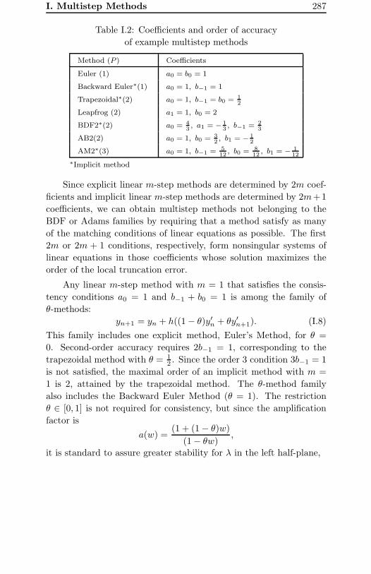
Four of our working example methods of Chapter 5 and three ad-

ditional methods discussed above fit into the linear 𝑚-step framework

with 𝑚 ≤ 2. Table I.2 summarizes the nonzero coefficients defining

these methods and identifies the value of 𝑃 for which the matching

conditions up to order 𝑃 are satisfied, but not the conditions of order

𝑃 + 1. For reference, the conditions for 𝑝 = 2, 3, and 4 are

𝑚−1∑𝑗=0

𝑗2𝑎𝑗 −𝑚−1∑𝑗=−1

2𝑗𝑏𝑗 = 1,

−𝑚−1∑𝑗=0

𝑗3𝑎𝑗 +

𝑚−1∑𝑗=−1

3𝑗2𝑏𝑗 = 1,

and𝑚−1∑𝑗=0

𝑗4𝑎𝑗 −𝑚−1∑𝑗=−1

4𝑗3𝑏𝑗 = 1,

respectively.


Table I.2: Coefficients and order of accuracy

of example multistep methods

Method (𝑃 ) Coefficients

Euler (1) 𝑎0 = 𝑏0 = 1

Backward Euler∗(1) 𝑎0 = 1, 𝑏−1 = 1

Trapezoidal∗(2) 𝑎0 = 1, 𝑏−1 = 𝑏0 =12

Leapfrog (2) 𝑎1 = 1, 𝑏0 = 2

BDF2∗(2) 𝑎0 =43, 𝑎1 = − 1

3, 𝑏−1 =

23

AB2(2) 𝑎0 = 1, 𝑏0 =32, 𝑏1 = − 1

2

AM2∗(3) 𝑎0 = 1, 𝑏−1 =512

, 𝑏0 =812

, 𝑏1 = − 112

∗Implicit method

Since explicit linear 𝑚-step methods are determined by 2𝑚 coef-

ficients and implicit linear 𝑚-step methods are determined by 2𝑚+1

coefficients, we can obtain multistep methods not belonging to the

BDF or Adams families by requiring that a method satisfy as many

of the matching conditions of linear equations as possible. The first

2𝑚 or 2𝑚 + 1 conditions, respectively, form nonsingular systems of

linear equations in those coefficients whose solution maximizes the

order of the local truncation error.

Any linear 𝑚-step method with 𝑚 = 1 that satisfies the consis-

tency conditions 𝑎0 = 1 and 𝑏−1 + 𝑏0 = 1 is among the family of

𝜃-methods:

𝑦𝑛+1 = 𝑦𝑛 + ℎ((1− 𝜃)𝑦′𝑛 + 𝜃𝑦′𝑛+1). (I.8)

This family includes one explicit method, Euler’s Method, for 𝜃 =

0. Second-order accuracy requires 2𝑏−1 = 1, corresponding to the

trapezoidal method with 𝜃 = 12 . Since the order 3 condition 3𝑏−1 = 1

is not satisfied, the maximal order of an implicit method with 𝑚 =

1 is 2, attained by the trapezoidal method. The 𝜃-method family

also includes the Backward Euler Method (𝜃 = 1). The restriction

𝜃 ∈ [0, 1] is not required for consistency, but since the amplification

factor is

𝑎(𝑤) =(1 + (1− 𝜃)𝑤)

(1− 𝜃𝑤),

it is standard to assure greater stability for 𝜆 in the left half-plane,


To obtain an explicit two-step method with local truncation error

of order 4 in this way, we look for a method of the form

𝑦𝑛+1 = 𝑎0𝑦𝑛 + 𝑎1𝑦𝑛−1 + ℎ(𝑏0𝑦′𝑛 + 𝑏1𝑦

′𝑛−1)

whose coefficients satisfy the four linear conditions 𝑎0+𝑎1 = 1, −𝑎1+

𝑏0 + 𝑏1 = 1, 𝑎1 − 2𝑏1 = 1, −𝑎1 + 3𝑏1 = 1. The method corresponding

to the unique solution of this system is

𝑦𝑛+1 = −4𝑦𝑛 + 5𝑦𝑛−1 + ℎ(4𝑦′𝑛 + 2𝑦′𝑛−1). (I.9)

We showed in Section 5.3 that (I.9) is not 0-stable. Another method

that is consistent, but not 0-stable, is

𝑦𝑛+1 = 3𝑦𝑛 − 2𝑦𝑛−1 − ℎ𝑦′𝑛. (I.9′)

We can confirm the instability by considering the roots of its char-

acteristic polynomial for 𝑤 = 0, 𝑝0(𝑟) = 𝜌(𝑟) = 𝑟2 − 3𝑟 + 2 =

(𝑟 − 1)(𝑟 − 2). Though this method does not satisfy the second-

order accuracy conditions, keeping the same 𝑎0 = 3, 𝑎1 = −2 and

modifying the derivative coefficients to 𝑏0 = 12 and 𝑏1 = − 3

2 yields a

method that would be second-order accurate were it not for the same

instability.

The connection between the truly unstable behavior of the meth-

od (I.10), 𝑦𝑛+1 = 3𝑦𝑛−2𝑦𝑛−1−ℎ𝑦′𝑛, and the roots of its characteristic

polynomial for 𝑤 = 0, 𝑝0(𝑟) = 𝜌(𝑟) = 𝑟2 − 3𝑟 + 2 = (𝑟 − 1)(𝑟 − 2), is

apparent. This also make it clear that we could extend the example to

have higher-order truncation error while retaining the same unstable

behavior by keeping the same 𝑎0 = 3, 𝑎1 = −2 but modifying the

derivative coefficients to 𝑏0 = 12 and 𝑏1 = − 3

2 .

To obtain an implicit two-step method with local truncation error

of order 5 in this way, we look for a method of the form

𝑦𝑛+1 = 𝑎0𝑦𝑛 + 𝑎1𝑦𝑛−1 + ℎ(𝑏−1𝑦′𝑛+1 + 𝑏0𝑦

′𝑛 + 𝑏1𝑦

′𝑛−1)

whose coefficients satisfy the five linear conditions 𝑎0+𝑎1 = 1, −𝑎1+

𝑏−1 + 𝑏0 + 𝑏1 = 1, 𝑎1 + 2𝑏−1 − 2𝑏1 = 1, −𝑎1 + 3𝑏−1 + 3𝑏1 = 1,

𝑎1+4𝑏−1−4𝑏1 = 1. The method corresponding to the unique solution


of this system is

𝑦𝑛+1 = 𝑦𝑛−1 + 2ℎ

(1

6𝑦′𝑛+1 +

4

6𝑦′𝑛 +

1

6𝑦′𝑛−1

), (I.10)

known as Milne’s corrector. We can also interpret this as integrating

quadratic interpolation of 𝑦′ at 𝑡𝑛+1, 𝑡𝑛, 𝑡𝑛−1 (the Simpson-parabolic

rule) to approximate the integral in

𝑦𝑛+1 − 𝑦𝑛−1 =

∫ 𝑡𝑛+1

𝑡𝑛−1

𝑦′(𝑠) 𝑑𝑠.

Additional families of methods may be obtained using approximations

of the integral in

𝑦𝑛+1 − 𝑦𝑛−𝑗 =

∫ 𝑡𝑛+1

𝑡𝑛−𝑗

𝑦′(𝑠) 𝑑𝑠

for larger values of 𝑗.

Seeking higher-order accuracy to improve efficiency does not as-

sure convergence. It can actually hinder it by compromising 0-stability.

This is the case even for the implicit methods, i.e., they do not always

have stability properties that are superior to those of explicit meth-

ods. In fact, for 𝑚 > 6, the backward difference methods, BDF𝑚,

are implicit methods with arbitrarily high formal accuracy, but they

are not even 0-stable.

If a general multistep method is applied to the model problem

𝑦′ = 𝜆𝑦 and we set 𝑤 = 𝜆ℎ, it takes the form of a homogeneous linear

difference equation

(1− 𝑏−1𝑤)𝑦𝑛+1 =

𝑚−1∑𝑗=0

(𝑎𝑗 + 𝑏𝑗𝑤)𝑦𝑛−𝑗 . (I.11)

We call the polynomial

𝑝𝑤(𝑟) = (1− 𝑏−1𝑤)𝑟𝑚 −

𝑚−1∑𝑗=0

(𝑎𝑗 + 𝑏𝑗𝑤)𝑟𝑚−(𝑗+1)


the characteristic polynomial of the multistep method (I.3). We also

define 𝜌(𝑟) and 𝜎(𝑟) by 𝑝𝑤(𝑟) = 𝜌(𝑟) + 𝑤𝜎(𝑟), so in particular,

𝜌(𝑟) = 𝑝0(𝑟) = 𝑟𝑚 −𝑚−1∑𝑗=0

𝑎𝑗𝑟𝑚−(𝑗+1).

When 𝑝𝑤(𝑟) has distinct roots 𝑟𝑗(𝑤), 𝑗 = 0, . . . ,𝑚 − 1, the general

solution of (I.11) is a linear combination

𝑦𝑛 =𝑚−1∑𝑗=0

𝑐𝑗𝑟𝑛𝑗 . (I.12)

If 𝑝𝑤(𝑟) has some multiple roots, we can index any set of them con-

secutively, 𝑟𝑗(𝑤) = ⋅ ⋅ ⋅ = 𝑟𝑗+𝑠(𝑤), in which case we replace the corre-

sponding terms in (I.12) by terms of the form 𝑐𝑗+𝑘𝑛𝑘𝑟𝑛𝑗 , 𝑘 = 0, . . . , 𝑠.

As 𝑤 → 0, the roots of 𝑟𝑗(𝑤) approach corresponding roots of

𝜌(𝑟). We can use the fact that some root 𝑟(𝑤) must approximate 𝑒𝑤 =

1 + 1𝑤 as 𝑤 → 0 as another derivation of the consistency conditions

(I.7). Since 𝑒0 = 1 must be a root of 𝑝0, 𝑝0(1) = 1 −∑𝑗 𝑎𝑗 = 0,

which is the zeroth-order consistency condition. Treating 𝑟(𝑤) as a

curve defined implicitly by the relation 𝑃 (𝑟, 𝑤) = 𝑝𝑤(𝑟) = 0 and

differentiate implicitly with respect to 𝑤 at (𝑟, 𝑤) = (1, 0), we obtain

−𝑚−1∑𝑗=−1

𝑏𝑗 + 𝑟′(𝑤)

⎛⎝𝑚−

𝑚−1∑𝑗=0

𝑎𝑗(𝑚− (𝑗 + 1))

⎞⎠ = 0.

Employing the zeroth-order consistency condition, factoring 𝑚 from

the second term, and setting 𝑟′(𝑤) = 1 yields the first-order consis-

tency condition of (I.7). This approach can be continued to any order.

Alternatively, we may consider to what degree 𝑟 = 𝑒𝑤 is a solution of

the characteristic equation 𝜌(𝑟) +𝑤𝜎(𝑟) = 0. The equations (I.5) for

𝑝 = 0, . . . , 𝑃 are equivalent to 𝜌(𝑒𝑤)+𝑤𝜎(𝑒𝑤) = 𝑂(𝑤𝑃+1) as 𝑤 → 0.

If we use 𝑤 = ln(𝑟) to write this in the form 𝜌(𝑟) + ln(𝑟)𝜎(𝑟) = 0,

they are also equivalent to

𝜌(𝑟) + ln(𝑟)𝜎(𝑟) = 𝐶∣𝑟 − 1∣𝑃+1 +𝑂(∣𝑟 − 1∣𝑃+2), (I.13)


as 𝑟 → 1 (so 𝑤 → 0). It is convenient to expand ln(𝑟) in powers of

𝑢 = 𝑟 − 1 near 𝑢 = 0, in which case (I.13) becomes

𝜌(1 + 𝑢) + ln(1 + 𝑢)𝜎(1 + 𝑢) = 𝐶∣𝑢∣𝑃+1 +𝑂(∣𝑢∣𝑃+2).

In terms of the coefficients 𝑎𝑗 and 𝑏𝑗 of the numerical method,

and using 𝑞 = 𝑚− 1 as before, this becomes

(1 + 𝑢)𝑚 − (𝑎0(1 + 𝑢)𝑞 + ⋅ ⋅ ⋅+ 𝑎𝑞)− (𝑢− 𝑢2

2+

𝑢3

3− ⋅ ⋅ ⋅ )

× (𝑏−1(1 + 𝑢)𝑚 + 𝑏0(1 + 𝑢)𝑞 + ⋅ ⋅ ⋅+ 𝑏𝑞) = 𝐶∣𝑢∣𝑃+1 +𝑂(∣𝑢∣𝑃+2).

(I.14)

The condition that the coefficient of the 𝑢𝑝 term on the left-hand

side vanishes is equivalent to the order 𝑝 matching condition we have

given above.

The competition between accuracy and stability is explained in

part by two results of Dahlquist that describe barriers to the order

of accuracy of multistep methods that satisfy certain stability condi-

tions. The first barrier gives the maximum order of a stable 𝑚-step

method. Specifying 𝑚− 1 nonprincipal roots of 𝜌(𝑟) that satisfy the

root condition is equivalent to specifying 𝑚− 1 real parameters that

describe some combination of real roots and complex conjugate pairs.

Along with 𝑟0 = 1, these determine the real coefficients 𝑎𝑗 through

𝜌(𝑟) = Π(𝑟 − 𝑟𝑗). Depending on whether the method is explicit or

implicit, this leaves 𝑚 or 𝑚+1 coefficients 𝑏𝑗 with which to satisfy the

accuracy conditions of order 𝑝 = 1, . . . , 𝑃 . If the method is explicit,

one would expect that this is possible through 𝑃 = 𝑚, and through

𝑃 = 𝑚+ 1 if the method is implicit. We know that these are attain-

able from the examples of AB2 and AM2, stable two-step methods

of order 2 and 3, respectively. In the explicit case, this bound turns

out to be correct in general, and also in the implicit case if 𝑚 is odd.

However, if 𝑚 is even, it is possible to satisfy one more additional

equation, i.e., there are stable implicit 𝑚-step methods with order

𝑚 + 2, but none higher. Milne’s corrector satisfies the root condi-

tion, so it is 0-stable and convergent. But, for arbitrarily small 𝑤

the magnitude of the root of 𝑝𝑤(𝑟) that approaches −1 as 𝑤 → 0

can exceed that of the principal root that approaches +1. Because of

this, it lacks a desirable property called relative stability, but it is still


0-stable and convergent. It is suggestive that this method contains

a form of the Simpson-parabolic integration method, an example of

the Newton-Cotes quadrature methods based on an odd number of

nodes. Due to symmetry, these quadrature methods attain an addi-

tional degree of accuracy over the number of nodes when the number

of nodes is odd.

The second barrier refers to methods that are A-stable, which

means that their region of absolute stability contains the entire left

half-plane, i.e., all 𝑤 ∈ C such that Re(𝑤) ≤ 0. Dahlquist showed

that any A-stable linear multistep method has order of accuracy less

than or equal to 2. Because of the usefulness of methods with large

regions of absolute stability, considerable effort has gone into finding

higher-order A(𝛼)-stable methods whose regions of absolute stability

contain large wedges symmetric about the negative real axis in the

left half-plane.

The analysis of propagation of errors for linear multistep meth-

ods involves issues arising from multiple initial values and modes of

amplification that are not present in one-step methods. When we

analyzed the error propagation of Euler’s Method, we saw that the

global error is bounded in terms of a sum of contributions arising from

initial error and local truncation error, interacting with the amplifica-

tion associated with the method. The portion of the bound resulting

from the local truncation error has order one less than that of the

local truncation error itself, while the portion resulting from the ini-

tialization error has the same order of the initialization error. The

heuristic explanation is that the number of steps in which truncation

errors are introduced grows in inverse proportion to the step size,

contributing a factor of ℎ−1. Initialization errors may be amplified

by some bounded constant, but they are introduced in a fixed number

of steps that are independent of ℎ. So the global order of accuracy

of one-step and 0-stable linear multistep methods is at most one less

than the order of the local truncation error. But initialization errors

are only introduced in a fixed number of steps that is independent of

ℎ, so their contribution to the global error has the same magnitude as

that of the initialization errors themselves. For the global order to be

as small as possible, the initial values must also be one less than the


order of the local truncation error; any more accuracy is wasted. For

one step methods, the initial value can be considered exact, since it is

given in the IVP, though even this value may include experimental or

computational errors. But for 𝑚-step methods with 𝑚 > 1, we must

use one-step methods to generate one or more additional values. Once

we have a second initial value, we could also use a two-step method to

generate a third, then a three-step method to generate a fourth, and

so on. No matter how we choose to do this, it is just the order of the

(local truncation) error of the initial values that limits the global error

of the solution. For this reason, it is sufficient to initialize a method

whose local truncation error has order 𝑃 + 1 using a method whose

local truncation error has order 𝑃 . For example, the local truncation

error of the leapfrog method has order 3. If 𝑦0 = 𝑦𝑜, the exact initial

value, and we use Euler’s Method, whose local truncation error has

order 2, to obtain 𝑦1 from 𝑦0, the resulting method has global order

of accuracy 2. If we use the midpoint method or Heun’s Method,

whose local truncation errors both have order 3, the global order of

accuracy of the resulting methods is still 2, no more accurate than

if we use Euler’s Method to initialize. But if we use a lower-order

approximation, 𝑦1 = 𝑦0, a method whose local truncation error has

order 1 and is not even consistent, the savings of one evaluation of

𝑓 degrades the convergence of all subsequent steps to global order 1.

As another example, the two-step implicit Adams-Moulton Method,

AM2, has local truncation error of order 4. If we initialize it with the

midpoint method or Heun’s Method, we achieve the greatest possible

global order of accuracy, 3. Initializing with RK4 will not improve

this behavior, and initializing with Euler’s Method degrades the or-

der to 2. So the reason for including initial errors in the analysis of

error propagation for one-step methods is clarified when we consider

multistep methods.

When 𝑦𝑛+1 is only defined implicitly, the ease with which we can

determine its value from 𝑦𝑛 (and previous values in the case of a

multistep method) is significant from both practical and theoretical

points of view. In the first place, a solution might not even exist for all

values of ℎ > 0. For a simple one-step method such as the Backward

Euler Method, it can fail to have a solution even for the linear equation


𝑦′ = 𝜆𝑦, 𝑦(0) = 𝑦𝑜, where it reduces to 𝑦𝑛+1(1 − 𝜆ℎ) = 𝑦𝑛, which

clearly has no solution if 𝜆ℎ = 1 and 𝑦𝑛 ∕= 0.

When 𝑏−1 ∕= 0, (I.3) can be considered as a family of fixed-point

equations 𝑦𝑛+1 = 𝑇 (𝑦𝑛+1, ℎ) depending on the parameter ℎ. If we let

𝑦𝑛+1∗ =

𝑚−1∑𝑗=0

𝑎𝑗𝑦𝑛−𝑗 , (I.15)

then 𝑦𝑛+1∗ = 𝑇 (𝑦𝑛+1

∗, 0). Using the Lipschitz continuity of 𝑓 with

respect to 𝑦 and the linearity of 𝑇 with respect to ℎ, we can show that

for sufficiently small ℎ, 𝑇 (⋅, ℎ) is a contraction that maps an interval

𝐼 containing 𝑦𝑛+1∗ into itself. By the contraction mapping principle,

for any 𝑦𝑛+1(0) in this interval, the iteration

𝑦𝑛+1(𝑘+1) = 𝑇 (𝑦𝑛+1

(𝑘), ℎ) (I.16)

converges linearly to a unique fixed point 𝑦𝑛+1, satisfying 𝑦𝑛+1 =

𝑇 (𝑦𝑛+1, ℎ), with rate

𝑏−1ℎ∣∂𝑓∂𝑦

(𝑦𝑛+1)∣ ≤ ∣𝑏−1ℎ𝐿∣. (I.17)

The situation for implicit Runge-Kutta Methods is more involved,

since each step requires the solution of a nonlinear system of equa-

tions, but the same principles can be extended to derive existence,

smooth dependence, and a convergence rate proportional to ℎ, when

ℎ is sufficiently small.

It is a key principle in the design, analysis, and implementation

of predictor-corrector methods that the convergence rate of the fixed-

point iteration (I.16) is proportional to ℎ. If we perform a single step

of an implicit method of order 𝑝 by iterating (I.16) to convergence,

the resulting 𝑦𝑛+1∞ has a local truncation error that behaves like

∣𝑦(𝑡𝑛+1)− 𝑦𝑛+1∞∣ ≈ 𝐶ℎ𝑃+1 as ℎ → 0. If we only iterate (I.16) so far

that ∣𝑦𝑛+1(𝑘)−𝑦𝑛+1

∞∣ ≈ 𝐶 ′ℎ𝑃+1 as ℎ → 0 as well, then using 𝑦𝑛+1(𝑘)

instead of 𝑦𝑛+1∞ should still result in a method with the same order.

We may do this in a variety of ways, but it is common to initial-

ize the iteration with an explicit method, called a predictor, whose

order is the same or one less than that of the implicit method, 𝑃 .


Each iteration of (I.16) is called a corrector step, and if our predic-

tor has global order 𝑃 − 1, its local truncation error will behave like

∣𝑦(𝑡𝑛+1) − 𝑦𝑛+1(0)∣ ≈ 𝐶𝑃ℎ

𝑃 . Since this dominates the local trun-

cation error of the corrector, ∣𝑦𝑛+1∞ − 𝑦𝑛+1

(0)∣ ≈ 𝐶𝑃ℎ𝑃 , it makes

sense to perform one corrector iteration. Due to the ℎ dependence of

the rate of convergence, ∣𝑦𝑛+1∞ − 𝑦𝑛+1

(1)∣ ≈ 𝐶𝐶ℎ𝑃+1 and therefore

∣𝑦(𝑡𝑛+1)− 𝑦𝑛+1(1)∣ ≈ 𝐶 ′

𝐶ℎ𝑃+1, and further iterations do not increase

the order of the local truncation error. If a predictor is already as ac-

curate as the implicit method, 𝑦(𝑡𝑛+1)− 𝑦𝑛+1(0) ≈ 𝐶 ′

𝑃ℎ𝑃+1, it would

seem pointless to iterate, since one iteration provides no improvement

in overall accuracy. At the opposite extreme, we could even initialize

with the constant method, 𝑦𝑛+1 = 𝑦𝑛, for which the local truncation

error ∣𝑦(𝑡𝑛+1)− 𝑦𝑛+1(0)∣ ≈ 𝑦′𝑛ℎ, and perform 𝑃 corrector iterations.

We now consider two simple concrete examples. The implicit

method we will use in the first example is the Backward Euler Method,

and in the second example we will use the trapezoidal method. We

will analyze both accuracy and stability for the model problem 𝑦′ =𝜆𝑦 in order to understand why it makes sense to correct to—or even

beyond—the maximal achievable accuracy of the method. One reason

is improvement in the region of absolute stability. The region of abso-

lute stability of the explicit method corresponding to 𝑦𝑛+1 = 𝑦𝑛+1(0)

gets deformed step by step into that of the implicit method corre-

sponding to 𝑦𝑛+1 = 𝑦𝑛+1∞. A second reason is that the difference

between 𝑦𝑛+1(0) and 𝑦𝑛+1

(1), obtained from a corrector of the same

order, can be used to estimate local errors with very little additional

computation, and this can be used to adjust the step-size automati-

cally and even change on the fly to an appropriate higher- or lower-

order method.

For the purpose of analyzing the local truncation error in both ex-

amples, we let 𝑦(𝑡𝑛+1) be the exact solution passing through (𝑡𝑛, 𝑦𝑛),

evaluated at 𝑡𝑛+1, so 𝑦(𝑡𝑛+1) = 𝑦𝑛𝑒𝜆ℎ =

∑∞𝑗=0

(𝜆ℎ)𝑗

𝑗! . The iteration

(I.16) corresponding to the Backward Euler Method is

𝑦𝑛+1(𝑘+1) = 𝑦𝑛 + ℎ𝑓(𝑡𝑛+1, 𝑦𝑛+1

(𝑘)).

For the model problem 𝑓(𝑡, 𝑦) = 𝜆𝑦, if we initialize the iteration

with 𝑦𝑛+1(0) = 𝑦𝑛 and perform no iterations, the local truncation


error behaves like 𝑦′(𝑡𝑛)ℎ = 𝜆ℎ𝑦𝑛 as ℎ → 0. If we iterate once,

𝑦𝑛+1(1) = (1 + 𝜆ℎ)𝑦𝑛, and the result is no different than if we had

applied one step of Euler’s Method, which has local truncation error

𝑦(𝑡𝑛+1) − 𝑦𝑛+1(1) ≈ 𝑦′′(𝑡𝑛)ℎ

2

2 = (𝜆ℎ)2

2 𝑦𝑛 as ℎ → 0. Another iter-

ation gives 𝑦𝑛+1(2) = (1 + 𝜆ℎ + (𝜆ℎ)2)𝑦𝑛, and we may also think

of this as using an Euler’s Method predictor followed by one Back-

ward Euler corrector step. The local truncation error 𝑦(𝑡𝑛+1) −𝑦𝑛+1

(2) ≈ −𝑦′′(𝑡𝑛)ℎ2

2 = − (𝜆ℎ)2

2 𝑦𝑛. This is to be expected since

after this iteration, 𝑦𝑛+1(2) is an 𝑂(ℎ3) approximation of the ap-

proximation 𝑦𝑛+1(∞) = (1 − 𝜆ℎ)−1𝑦𝑛 =

∑∞𝑗=0(𝜆ℎ)

𝑗 whose terms to

order ℎ2 agree with those of 𝑦𝑛+1(2) above and only agree to order

ℎ with 𝑦(𝑡𝑛+1). Therefore, 𝑦𝑛+1(2) shares the same error behavior

as 𝑦(𝑡𝑛+1) − 𝑦𝑛+1(∞) ≈ −𝑦′′(𝑡𝑛)ℎ

2

2 = − (𝜆ℎ)2

2 𝑦𝑛 as ℎ → 0. Better

approximations of 𝑦𝑛+1(∞) are not better approximations of 𝑦(𝑡𝑛+1).

The benefits of these iterations are increased stability and error

estimation. Euler’s Method is never absolutely stable for 𝑤 = 𝜆ℎ

on the imaginary axis, since ∣1 + 𝑤∣ > 1 for 𝑤 = 𝑎𝑖, 𝑎 ∕= 0. The

amplification factor corresponding to 𝑦𝑛+1(2), 𝑎(𝑤) = 1 + 𝑤 + 𝑤2,

satisfies ∣1+𝑤+𝑤2∣ ≤ 1 for 𝑤 = 𝑎𝑖, 𝑎 ∈ [−1, 1]. Also, we can subtract

𝑦(𝑡𝑛+1)− 𝑦𝑛+1(2) ≈ −𝑦′′(𝑡𝑛)ℎ

2

2 from 𝑦𝑛+1(2) − 𝑦𝑛+1

(1) ≈ 𝑦′′(𝑡𝑛)ℎ2, to

obtain an estimate of the local truncation error in terms of computed

quantities, 𝑦(𝑡𝑛+1) − 𝑦𝑛+1(2) ≈ 1

2 (𝑦𝑛+1(2) − 𝑦𝑛+1

(1)) as ℎ → 0. If

this error exceeds a certain bound, we may decide to reduce the step

size, or we can use these quantities once more to increase the order of

our method by canceling the leading terms in their errors (a process

known as extrapolation). In this case, we can define a new predictor

from their mean, 𝑦𝑛+10 = 1

2 (𝑦𝑛+1(2) − 𝑦𝑛+1

(1)), and expect its local

truncation error to behave as ℎ3 as ℎ → 0. This is indeed the case, as

this is just Heun’s Method. In conjunction with an implicit method

with second-order accuracy, we could then continue the process. For

this reason, we briefly perform a similar analysis of a trapezoidal

corrector.

The iteration (I.16) corresponding to the trapezoidal method is

𝑦𝑛+1(𝑘+1) = 𝑦𝑛 +

ℎ

2(𝑓(𝑡𝑛, 𝑦𝑛) + 𝑓(𝑡𝑛+1, 𝑦𝑛+1

(𝑘))).


For the model problem 𝑓(𝑡, 𝑦) = 𝜆𝑦, if we initialize the iteration

with 𝑦𝑛+1(0) = 𝑦𝑛 and perform no iterations, the local truncation

error behaves like 𝑦′(𝑡𝑛)ℎ = 𝜆ℎ𝑦𝑛 as ℎ → 0. If we iterate once,

𝑦𝑛+1(1) = (1+𝜆ℎ)𝑦𝑛 and the result is still no different than if we had

applied one step of Euler’s Method, which has local truncation error

𝑦(𝑡𝑛+1) − 𝑦𝑛+1(1) ≈ 𝑦′′(𝑡𝑛)ℎ

2

2 = (𝜆ℎ)2

2 𝑦𝑛 as ℎ → 0. But this time,

another iteration gives 𝑦𝑛+1(2) = (1 + 𝜆ℎ + (𝜆ℎ)2

2 )𝑦𝑛, and we may

also think of this as using an Euler’s Method predictor followed by

one trapezoidal corrector step, i.e., Heun’s Method. The local trun-

cation error 𝑦(𝑡𝑛+1) − 𝑦𝑛+1(2) ≈ −𝑦′′(𝑡𝑛)ℎ

3

6 = (𝜆ℎ)3

6 𝑦𝑛. Beyond the

first iteration, 𝑦𝑛+1(𝑘) attains the same accuracy of 𝑦𝑛+1

(∞); better

approximations of 𝑦𝑛+1(∞) are not better approximations of 𝑦(𝑡𝑛+1).

The asymptotic form of the third-order local error terms for Heun’s

Method, a Runge-Kutta Method, depends on the problem to which it

is applied. For the model problem, the asymptotic form of the local

error is identical to that of the trapezoidal method, so they cannot

be used together even in this situation for local error estimation with

the Milne device.

For any 𝑚 > 0, the AB𝑚 predictor, AM𝑚 − 1 corrector pair

has good stability and convergence properties and does satisfy the

common order requirements of the Milne device.

Using a predictor with one iteration of a corrector is sometimes

denoted 𝑃𝐶 or 𝑃𝐶1, with 𝑛 corrector iterations, 𝑃𝐶𝑛, and correc-

tor iterations to convergence, 𝑃𝐶∞. Redefining 𝑃 = 𝑃𝐶𝑛−1 to be

a new predictor turns 𝑃𝐶𝑛 into 𝑃𝐶. The evaluations of 𝑓(𝑡, 𝑦) in

the definition of the method are sometimes denoted as a distinct step

with the letter 𝐸, especially when expensive updates can be omitted

and iterations can be usefully performed with prior evaluations. This

is somewhat analogous to using a single Jacobian for multiple iter-

ations of Newton’s Method for the reduction of operations from 𝑁3

to 𝑁2. When all evaluations are performed, the method is denoted

𝑃𝐸(𝐶𝐸)𝑛, though there are many variations possible. If absolute

stability of the implicit method is essential for the particular problem

at hand, e.g., when an A-stable method is required, more efficient ap-

proaches to computing 𝑦𝑛+1 (e.g., Newton or quasi-Newton Methods)

should be implemented for quadratic rather than linear convergence.


This highlights a perspective that the predictor-corrector idea is not

only about finding the solution of the implicit stepping method—that

may be found by more efficient means. Rather, it is about designing

efficient intermediate explicit methods with enhanced stability and

error estimation properties. The use of two methods of common or-

der that share a substantial portion of their computational effort for

automatic step-size control is not limited to explicit-implicit pairs.

The same idea is used in one-step explicit methods, e.g., the Runge-

Kutta-Fehlberg pair.

We conclude with some general remarks on the theoretical and

practical effects of stability and instability for multistep methods.

The growth of errors in numerical approximations obtained from lin-

ear multistep methods is governed by a difference inequality consisting

of a homogeneous error amplification term correlated with the stabil-

ity properties of the method and an inhomogeneous error-forcing term

correlated with the local truncation error. The contribution from er-

ror amplification is governed by the same recurrence that determines

the stability of the method and in particular by the behavior of the

method on the model problem 𝑦′ = 𝜆𝑦 where 𝜆 = 𝐿, the Lipschitz

constant for 𝑓 .

The most fundamental result in the theory of linear multistep

methods is known as Dahlquist’s Equivalence Theorem. This theorem

relates the root condition and convergence as follows. Let (I.3) be a

consistent 𝑚-step method applied to the well-posed IVP (I.1), with

initial values 𝑦0, . . . , 𝑦𝑚−1 approaching 𝑦𝑜 as ℎ → 0. The method

is convergent if and only if 𝜌(𝑟) satisfies the root condition. Fur-

thermore, if the local truncation error defined in (I.4) satisfies ∣𝜖𝑛∣ ≤𝐶𝑇ℎ

𝑃+1 and the initial errors 𝑒𝑗,ℎ = 𝑦𝑗,ℎ − 𝑦(𝑡𝑗), 𝑗 = 0, . . . ,𝑚 − 1,

satisfy

max𝑗=0,... ,𝑚−1

∣𝑒𝑗,ℎ∣ ≤ 𝐶𝐼ℎ𝑃 ,

then

max0≤𝑛ℎ≤𝑇

∣𝑦𝑛,ℎ − 𝑦(𝑡𝑛)∣ ≤ 𝐶𝐺ℎ𝑃

as ℎ → 0. In other words, if the local truncation error has order 𝑃+1,

the initial error only needs to have order 𝑃 for the global convergence


to have order 𝑃 . A proof that applies to an even more general class

of methods may be found in [IK]. In the much greater generality

of linear finite difference methods for partial differential equations,

the fact that stability and consistency together are both necessary

and sufficient for convergence is the content of the important Lax-

Richtmyer Equivalence Theorem [LR].

There are several other more stringent conditions that have been

developed to distinguish the behavior observed in convergent linear

multistep methods. The strong root condition says that except for

𝑟0, the roots of 𝜌(𝑟) are all inside the open unit disc, a condition

that, as the name suggests, clearly implies the root condition. By

continuity, for sufficiently small ℎ, the nonprincipal roots 𝑟𝑗(𝑤) of

𝜌(𝑟) + 𝑤𝜎(𝑟) will also have magnitude less than 1. If the coefficients

of an 𝑚-step method with 𝑚 > 1 satisfy 𝑎𝑗 = 0 for 𝑗 < 𝑚 − 1, so

𝑎𝑚−1 = 1 for consistency, it cannot satisfy the strong root condition,

since the roots of 𝜌(𝑟) = 𝑟𝑚 − 1 are all of the form 𝑟𝑗 = 𝑒2𝜋𝑗/𝑚, 𝑗 =

0, . . . ,𝑚 − 1. This class includes the leapfrog method and Milne’s

corrector. Even if the strong root condition is not satisfied, we can

require that for sufficiently small ℎ, the parasitic roots of 𝑝𝑤(𝑟) have

magnitudes less than or equal to the magnitude of the principal root,

a condition called relative stability. In this case, parasitic roots can

only grow exponentially when the principal root is growing faster

exponentially, making them less of a concern. The term weak stability

is used to describe a method that is stable but not relatively stable.

Since the leapfrog method satisfies the root condition and we have

shown that as ℎ → 0, the parasitic root of the leapfrog method has

magnitude greater than its principal root, the leapfrog method is

weakly stable and demonstrates that the root condition cannot imply

relative stability. However, the continuity argument that shows that

the strong root condition implies the root condition can be used just as

easily to show that the strong root condition implies relative stability.

By the observation above, the consistent two-step method 𝑦𝑛+1 =

𝑦𝑛−1 +2ℎ𝑦′𝑛−1 cannot satisfy the strong root condition. But since its

characteristic polynomial is

𝑟2 − (1 + 2𝑤) = (𝑟 −√1 + 2𝑤)(𝑟 +

√1 + 2𝑤),


its principal and parasitic roots have the same magnitude and it is

relatively stable. This shows that relative stability is strictly weaker

than the strong root condition.

For Euler’s Method, the Backward Euler Method, and the trape-

zoidal method, 𝜌(𝑟) = 𝑟 − 1. Since there are no nonprincipal roots,

they satisfy the strong root condition, the root condition, and the

relative stability condition by default. Both the explicit and the im-

plicit 𝑚-step Adams Methods, AB𝑚 and AM𝑚, are designed to have

𝜌(𝑟) = 𝑟𝑚 − 𝑟𝑚−1 = (𝑟− 1)𝑟𝑚−1, so that all parasitic roots are zero!

These methods satisfy the strong root condition, as nicely as possible.

For BDF2, 𝜌(𝑟) = 𝑟2 − 43𝑟 +

13 = (𝑟 − 1)(𝑟 − 1

3 ) satisfies the strong

root condition. For higher 𝑚, BDF𝑚 is designed to have order of

accuracy 𝑚 if the method is convergent. However, these methods are

only 0-stable for 𝑚 ≤ 6, so BDF𝑚 is not convergent for 𝑚 ≥ 7.

If we apply Milne’s corrector, the implicit two-step method having

maximal local truncation error, to the model problem 𝑦′ = 𝜆𝑦, it takes

the form

𝑦𝑛+1 = 𝑦𝑛−1 + (𝑤

3𝑦𝑛+1 +

4𝑤

3𝑦𝑛 +

𝑤

3𝑦𝑛−1).

Solutions are linear combinations 𝑦𝑛 = 𝑐+𝑟++𝑐−𝑟− where 𝑟± are the

roots of

𝑝𝑤(𝑟) = (1− 𝑤/3)𝑟2 − (4𝑤/3)𝑟 − (1 + 𝑤/3).

By setting 𝑢 = 𝑤/3 and multiplying by 1/(1 − 𝑢) = 1 + 𝑢 + ⋅ ⋅ ⋅ , tofirst order in 𝑢, these roots satisfy

𝑟2 − 4𝑢(1 + ⋅ ⋅ ⋅ )𝑟 − (1 + 2𝑢+ ⋅ ⋅ ⋅ ) = 0

or

𝑟± = 2𝑢±√4𝑢2 + 1 + 2𝑢.

Using the binomial expansion (1+ 2𝑢)1/2 ≈ 1+𝑢+ ⋅ ⋅ ⋅ , to first order

in 𝑢, 𝑟+ ≈ 1 + 3𝑢 and 𝑟− ≈ −1 + 𝑢. The root ≈ 1 + 3𝑢 = 1 + 𝜆ℎ

approximates the solution of the model problem 𝑦′ = 𝜆𝑦. As 𝜆ℎ → 0

in a way that 𝑢 in a neighborhood of the negative real axis near

the origin, the other root ≈ −1 + 𝑢 has magnitude greater than 1,

showing that Milne’s Method corrector is not relatively stable. Like

the leapfrog method, it satisfies the root condition, so it is stable, but


only weakly stable. So even a convergent implicit method can have

worse stability properties than a convergent explicit method.

We can summarize the relationship among various types of sta-

bility for multistep methods and their consequences as follows:

strong root condition ⇒ relative stability ⇒ root condition,

absolute stability for 𝑤 = 0 ⇒ root condition ⇔ 0-stability,

consistency + root condition ⇔ convergence,

𝑃 th-order formal accuracy+root condition ⇔ 𝑃 th-order convergence.

We conclude by cautioning the reader that many examples in

Chapter 5 show that the behavior of a method is not determined by

either the order of its local truncation error or by the rather loose

bounds provided by 0-stability. 0-stability is certainly important,

helping us to avoid nonconvergent methods, a caveat that cannot be

overemphasized. Convergence and stability are a minimal but im-

portant requirement for a useful method. Along with the order of

accuracy, the actual performance of a method is more closely corre-

lated with its absolute stability with respect to modes present in the

ODE.

⊳Exercise I–1. Determine the regions of absolute stability for

BDF2, AM2, and AM2. For implicit methods, it may be advanta-

geous to consider the fact that if 𝑟 ∕= 0 is a root of 𝑎𝑟2 + 𝑏𝑟 + 𝑐, then

𝑠 = 1𝑟 is a root of 𝑐𝑠2 + 𝑏𝑠+ 𝑎.

Appendix J

Iterative Interpolationand Its Error

In this appendix we give a brief review of iterative polynomial inter-

polation and corresponding error estimates used in the development

and analysis of numerical methods for differential equations.

The unique polynomial of degree 𝑛,

𝑝𝑥0,... ,𝑥𝑛(𝑥) =

𝑛∑𝑗=0

𝑎𝑗𝑥𝑗 , (J.1)

that interpolates a function 𝑓(𝑥) at 𝑛+ 1 points,

𝑝𝑥0,... ,𝑥𝑛(𝑥𝑖) = 𝑦𝑖 = 𝑓(𝑥𝑖), 0 ≤ 𝑖 ≤ 𝑛, (J.2)

can be found by solving simultaneously the (𝑛 + 1) × (𝑛 + 1) linear

system of equations for the 𝑛 + 1 unknown coefficients 𝑎𝑗 given by

(J.2). It can also be found using Lagrange polynomials

𝑝𝑥0,... ,𝑥𝑛(𝑥) =

𝑛∑𝑖=0

𝑦𝑖𝐿𝑖,𝑥0,... ,𝑥𝑛(𝑥) (J.3)

where

𝐿𝑖,𝑥0,... ,𝑥𝑛(𝑥) =

∏0≤𝑗≤𝑛,𝑗 ∕=𝑖

(𝑥− 𝑥𝑗)

(𝑥𝑖 − 𝑥𝑗). (J.4)

Here, we develop 𝑝𝑥0,... ,𝑥𝑛(𝑥) inductively, starting from 𝑝𝑥0

(𝑥) = 𝑦0and letting

𝑝𝑥0,... ,𝑥𝑗+1(𝑥)

= 𝑝𝑥0,... ,𝑥𝑗(𝑥) + 𝑐𝑗+1(𝑥− 𝑥0) ⋅ ⋅ ⋅ (𝑥− 𝑥𝑗), 𝑗 = 0, . . . , 𝑛− 1

(J.5)

303

304 J. Iterative Interpolation and Its Error

(so that each successive term does not disturb the correctness of

the prior interpolation) and defining 𝑐𝑗+1 so that 𝑝𝑥0,... ,𝑥𝑗+1(𝑥𝑗+1) =

𝑦𝑗+1, i.e.,

𝑐𝑗+1 =𝑦𝑗+1 − 𝑝𝑥0,... ,𝑥𝑗

(𝑥𝑗+1)

(𝑥𝑗+1 − 𝑥0)= 𝑓 [𝑥0, . . . , 𝑥𝑗+1]. (J.6)

Comparing (J.6) with (J.3), (J.4) gives an alternate explicit expres-

sion for 𝑓 [𝑥0, . . . , 𝑥𝑛], the leading coefficient of the polynomial of

degree 𝑛 that interpolates 𝑓 at 𝑥0, . . . , 𝑥𝑛:

𝑓 [𝑥0, . . . , 𝑥𝑛] =

𝑛∑𝑖=0

𝑓(𝑥𝑖)∏𝑗 ∕=𝑖(𝑥𝑖 − 𝑥𝑗)

(J.7)

from which follows the divided difference relation

𝑓 [𝑥0, . . . , 𝑥𝑛] =𝑓 [𝑥0, . . . , 𝑥𝑗 , . . . 𝑥𝑛] − 𝑓 [𝑥0, . . . , 𝑥𝑖 . . . , 𝑥𝑛]

𝑥𝑖 − 𝑥𝑗(J.8)

(where ˆ indicates omission).

For our purposes, we want to estimate 𝑝𝑥0,... ,𝑥𝑛(𝑡) − 𝑓(𝑡), and

to do so, we simply treat 𝑡 as the next point at which we wish to

interpolate 𝑓 in (J.5):

𝑝𝑥0,... ,𝑥𝑛(𝑡) + 𝑓 [𝑥0, . . . , 𝑥𝑛, 𝑡](𝑡− 𝑥0) ⋅ ⋅ ⋅ (𝑡− 𝑥𝑛) = 𝑓(𝑡)

or

𝑝𝑥0,... ,𝑥𝑛(𝑡)− 𝑓(𝑡) = 𝑓 [𝑥0, . . . , 𝑥𝑛, 𝑡](𝑡− 𝑥0) ⋅ ⋅ ⋅ (𝑡− 𝑥𝑛). (J.9)

Finally, we estimate the coefficient 𝑓 [𝑥0, . . . , 𝑥𝑛, 𝑡] using several appli-

cations of Rolle’s Theorem. Since 𝑝𝑥0,... ,𝑥𝑛,𝑡(𝑥)=𝑓(𝑥) or 𝑝𝑥0,... ,𝑥𝑛,𝑡(𝑥)

− 𝑓(𝑥) = 0 at 𝑛 + 2 points 𝑥0, . . . , 𝑥𝑛, 𝑡, Rolle’s Theorem says that

𝑝′𝑥0,... ,𝑥𝑛,𝑡(𝑥) − 𝑓 ′(𝑥) = 0 at 𝑛 + 1 points, one in each open interval

between consecutive distinct points of 𝑥0, . . . , 𝑥𝑛, 𝑡. Repeating this

argument, 𝑝′′𝑥0,... ,𝑥𝑛,𝑡(𝑥) − 𝑓 ′′(𝑥) = 0 at 𝑛 points on the intervals be-

tween the points described in the previous stage, and repeating this

𝑛− 1 more times, there is one point 𝜉 in the interior of the minimal

closed interval containing all of the original points 𝑥0, . . . , 𝑥𝑛, 𝑡 at

which

𝑝(𝑛+1)𝑥0,... ,𝑥𝑛,𝑡(𝜉)− 𝑓 (𝑛+1)(𝜉) = 0. (J.10)

J. Iterative Interpolation and Its Error 305

But because 𝑓 [𝑥0, . . . , 𝑥𝑛, 𝑡] is the leading coefficient of the polyno-

mial 𝑝𝑥0,... ,𝑥𝑛,𝑡(𝑥) of degree 𝑛 + 1 that interpolates 𝑓 at the 𝑛 + 2

points 𝑥0, . . . , 𝑥𝑛, 𝑡, if we take 𝑛 + 1 derivatives, we are left with a

constant, that leading coefficient times (𝑛+ 1)!:

𝑝(𝑛+1)𝑥0,... ,𝑥𝑛,𝑡(𝑥) = (𝑛+ 1)!𝑓 [𝑥0, . . . , 𝑥𝑛, 𝑡]. (J.11)

Combining this with (J.10) gives

𝑓 [𝑥0, . . . , 𝑥𝑛, 𝑡] =𝑓 (𝑛+1)(𝜉)

(𝑛+ 1)!(J.12)

where 𝜉 in the interior of the minimal closed interval containing all

of the original points 𝑥0, . . . , 𝑥𝑛, 𝑡, and substituting into (J.9) yields

the basic interpolation error estimate:

𝑝𝑥0,... ,𝑥𝑛(𝑡)− 𝑓(𝑡) =

𝑓 (𝑛+1)(𝜉)

(𝑛+ 1)!(𝑡− 𝑥0) ⋅ ⋅ ⋅ (𝑡− 𝑥𝑛). (J.13)

For 𝑛 = 0 this recovers the mean value theorem

𝑓(𝑡)− 𝑓(𝑥0)

𝑡− 𝑥0= 𝑓 ′(𝜉) (J.14)

for some 𝜉 ∈ (𝑥0, 𝑡).

Since many multistep methods involve simultaneous interpola-

tion of 𝑦 and 𝑦′ at 𝑡𝑛, . . . , 𝑡𝑛−𝑚+1, to treat these, we would want

to have the corresponding estimates for osculatory interpolation that

can be obtained by letting pairs of interpolation points coalesce. In

the simplest cases, for two points, this process recovers the tangent

line approximation and estimate

𝑓 [𝑥0] + 𝑓 [𝑥0, 𝑥0](𝑥− 𝑥0) = 𝑓(𝑥0) + 𝑓 ′(𝑥0)(𝑥− 𝑥0).

For four points, it recovers the cubic spline interpolation approx-

imating a function and its derivative at two points.

multistep methods - richard palais' home...

Documents