Multiple Eisenstein series, multiple divisor functions andapplications to multiple q-zeta values

Ulf Kühn (Hamburg)

joint work with Henrik Bachmann arXiv:1309.3920 [math.NT]

1 / 39

Per

iod

po

lyn

om

ials

modular forms

(2⇡i)

�2k

G

2k

(⌧) =

⇣(2k)

(2⇡i)

2k + [2k] 2 M

2k

(Sl

2

(Z),Q)

� 2 S

12

(Sl

2

(Z),Q)

Dimensions: d

k,l

= dimQ gr

L

l

M

k

(Sl

2

(Z),Q)

Pk,l

d

k,l

x

k

y

l

= 1 +

x

4

1�x

2 y +

x

12

(1�x

4)(1�x

6)

y

2

multiple divisor functions

[s

1

, ..., s

l

] :=

1

(s1�1)!...(sl�1)!

Pm1>···>ml>0

d1,...,dl>0

d

s1�1

1

. . . d

sl�1

l

q

m1d1+···+mldl 2 Q[[q]], Derivation d := q

d

dq

Relations:

[4] + 2[3]� 1

6

[2]� 4[3, 1] = d[2] = 2[4] + [3] +

1

6

[2]� 2[2, 2]� 2[3, 1]

Identities:

d[1] = [3] +

1

2

[2]� [2, 1]

[2, 3] + [3, 2] + [5]� 1

12

[3] = [2] · [3] = [2, 3] + 3[3, 2] + 6[4, 1] + d[3]� 3[4]

1

2

6·5·691� = 168[5, 7] + 150[7, 5] + 28[9, 3]� 5197

691

[12]� 7

120

[8] +

187

6048

[6]� 83

14400

[4] +

1

1408

[2]

multiple Eisenstein series

G

s1,...,sl(⌧) =

Pm1⌧+n1>...>ml⌧+nl>0

1

(m1⌧+n1)s1 ·...·(ml⌧+nl)

sl

Fourier expansion:

G

4,4

(⌧) = ⇣(4, 4) + 20⇣(6)(2⇡i)

2

[2] + 3⇣(4)(2⇡i)

4

[4] + (2⇡i)

8

[4, 4]

Identities:

G

4

(⌧) ·G6

(⌧)

stu✏e

= G

4,6

(⌧) +G

6,4

(⌧) +G

10

(⌧)

multiple zeta values

⇣(s

1

, ..., s

l

) =

Pn1>n2>...>nl>0

1

n

s11 ...n

sll

Relations:

⇣(3)

eds

= ⇣(2, 1)

⇣(2, 3) + ⇣(3, 2) + ⇣(5)

stu✏e

= ⇣(2) · ⇣(3) shu✏e

= ⇣(2, 3) + 3⇣(3, 2) + 6⇣(4, 1)

5197

691

⇣(12)

exotic

= 168⇣(5, 7) + 150⇣(7, 5) + 28⇣(9, 3)

Z

k

(f(q)) = lim

q!1

�(1� q)

k

f(q)

�

Image:

Z

s1+...+sl([s1,...,sl]) = ⇣(s

1

,...,s

l

)

Kernel:

[2], d[1] 2 kerZ

3

[3], [4], d[3] 2 kerZ

5

� 2 kerZ

12

Zk

1

2 / 36

74-

( x' 4×4×4×104# Eisenstein

series of # cusp forms= # hi

. indep.weights Eaten

Multiple zeta values

DefinitionLet s

1

� 2, s2

, ..., s

l

� 1 be natural numbers, then we call sums of the type

⇣(s1

, ..., s

l

) =X

n1>...>nl>0

1

n

s11

. . . n

sll

a multiple zeta value (MZV) of weight s1

+ ...+ s

l

and depth l.

The product of two MZV can be expressed as a linear combination of MZV with the sameweight (stuffle relation). e.g:

⇣(r) · ⇣(s) = ⇣(r, s) + ⇣(s, r) + ⇣(r + s) .

MZV can be calculated by iterated integrals. This gives another way (shuffle relation) toexpress the product of two MZV as a linear combination of MZV.

These two ways to express products give a lot ofQ-relations between MZV (double shufflerelations).

3 / 39

FI cnn.us , = Eo tr . I

,

Ems = Emtstan,

mostIEm,

# r

Multiple zeta-values

Example:

⇣(2, 3) + 3⇣(3, 2) + 6⇣(4, 1)shuffle= ⇣(2) · ⇣(3) stuffle

= ⇣(2, 3) + ⇣(3, 2) + ⇣(5) .

=) 2⇣(3, 2) + 6⇣(4, 1)double shuffle

= ⇣(5) .

But there are more relations between MZV. e.g.:

⇣(2, 1) = ⇣(3).

These follow from the "extended double shuffle relations" where one use the same combinatoricsas above for "⇣(1) · ⇣(2)" in a formal setting. The extended double shuffle relations areconjectured to give all relations between MZV.

4 / 39

Let Az

be a finite alphabet {z1

, z

2

, z

3

, ...}. A word is an ordered sequence w = z

i1 ...zil ofelements taken from A

z

, with repetition allowed. We include the empty word ; (or 1). We use theconcatenation product w · w0 and denote by A⇤

z

the set of all words. We take A⇤z

as a basis ofthe vector spaceQ < A

z

> of noncommutative polynomials. The concatenation of wordsdefines by linearity a multiplication onQ < A

z

>.

DefinitionThe stuffle product ⇤ onQ < A

z

> is defined by linear extension of the recursion given by

1 ⇤ w = w ⇤ 1 = w

for all w 2 A⇤z

and for words w,w0 and letters z1

, z

j

by

z

i

w ⇤ zj

w

0 = z

i1 · (w ⇤ zj

w

0) + z

j

· (zi

w ⇤ w0) + z

i+j

· (w ⇤ w0).

Proposition (Hoffmann)

The algebra�Q < A

z

>, ⇤�

is a commutative and associativeQ-algebra.

The stuffle product is an example for a quasi-shuffle product.

5 / 39

:wi general↳ing

of. it x A → ItC ti

c Zj I →

fc2.it;)

DefinitionWe denote by MZ 2 R theQ-subalgebra generated by multiple zeta values.

Theorem (Hoffmann)There is a unique homomorphism ofQ-algebras

⇣

⇤ :�Q < A

z

>, ⇤�! MZ

such that ⇣(z1

) = 0 and for all words w = z

i1 ...zil with i1

� 2

⇣

⇤(zi1 ...zil) = ⇣(s

i1 , ..., sil).

Remark

There is also a similar homomorphism ⇣

9

:�Q < {x, y} >,

9 � ! MZ which can be used

to describe the shuffle product. The comparison of ⇣⇤ and ⇣

9

, then leads to the extendeddouble shuffle relations.

6 / 39

Zi Zi * Zr = Zi I tj # Ze ) - I 2-e Cti 2-

j * 11

+ Z

itel Zi HI )

= zu C t; * Zu ) t Ze Zi 2

j+

kiteZi

}*

C Zi * 2- ; ) =3#

C Zizi t Zi Zi t Zing )= 3 c sie Si I t 3 C Sie Snl t 3C Siti )

Dimension conjectures for MZConsider the formal powerseries

E2

(x) =x

2

1�x

2 = x

2 + x

4 + x

6 + ... "even zetas",

O3

(x) =x

3

1�x

2 = x

3 + x

5 + x

7 + ... "odd zetas",

S(x) =x

12

(1�x

4)(1�x

6)

= x

12 + x

16 + x

18 + ... "period polynomials".

Broadhurst-Kreimer ConjectureTheQ-algebra MZ of multiple zeta values is a free polynomial algebra, which is graded for theweight and filtered for the depth ("depth drop for even zetas"). The numbers g

k,l

of generators inweight k � 3 and depth l are determined by

BK(x, y) =X

k,l�0

dimQ⇣grW,D

k,l

MZ⌘x

k

y

l =⇣1 + E

2

(x) y⌘ Y

k�3,l�1

1�1� x

k

y

l

�gk,l

where

BK(x, y) =⇣1 + E

2

(x)y⌘ 1

1� O3

(x)y + S(x)y2 � S(x)y4.

7 / 39

H,!

QE 31213 )

Dimension conjectures for MZ

Zagier’s ConjectureThe following identities hold:

Zag(x) =X

k�0

dimQ⇣grW

k

MZ⌘x

k =1

1� x

2 � x

3

.

Zagier’s conjecture is implied by Broadhurst-Kreimer’s conjecture. In order to neglect the depthwe just have to set y = 1 and get

Zag(x) = BK(x, 1) =1 + E

2

(x)

1� O3

(x)=

1 + x

2

1�x

2

1� x

3

1�x

2

=1

1� x

2 � x

3

.

Brown’s TheoremTheQ-vector space of multiple zeta values is spanned by the "23"-MZV’s, e.g. by those⇣(s

1

, ..., s

l

) with si

2 {2, 3}.

By Brown’s theorem the dimensions in Zagier’s conjecture are the maximal possible ones.

8 / 39

Theorem (Gangl&Kaneko&Zagier)

(i) The values ⇣(odd, odd) of weight k satisfy at least dimS

k

linearly independent relations,where S

k

denotes the space of cusp forms of weight k on Sl2

(Z).

(ii) For each even period polynomial an "exotic" relation as in (i) can be constructed.

Example. For k = 12 and k = 16, i.e. the first weights for which there are non-zero cusp forms,we have the identities

28⇣(9, 3) + 150⇣(7, 5) + 168⇣(5, 7) =5197

691⇣(12)

66⇣(13, 3) + 375⇣(11, 5) + 686⇣(9, 7) + 675⇣(7, 9) + 396⇣(5, 11) =78967

3617⇣(16).

9 / 39

Multiple q-zeta values

Many of the most basic concepts in mathematics have so-called q-analogues, where q is a formalvariable such that the specialisation q = 1 recovers the usual concept. Attributed to Gauss are theq-integers

{n}q

= 1 + q + . . .+ q

n�1 =1� q

n

1� q

.

We will study the following q-analogues of multiple zeta values.

Definition [(modified) multiple q-zeta-value]

For s1

, . . . , s

l

� 1 and polynomials Q1

(t) 2 tQ[t] and Q2

(t) . . . , Ql

(t) 2 Q[t] we define

⇣

q

(s1

, . . . , s

l

;Q1

, . . . , Q

l

) =X

n1>···>nl>0

Q

1

(qn1) . . . Ql

(qnl)

(1� q

n1)s1 · · · (1� q

nl)sl2 Q[[q]].

Such series can be seen as a q-analogue of multiple zeta values, since we have for s1

> 1

limq!1

(1� q)s1+···+sl⇣

q

(s1

, . . . , s

l

;Q1

, . . . , Q

l

) = Q

1

(1) . . . Ql

(1) · ⇣(s1

, . . . , s

l

) .

Observe, just replacing n by {n}q

in multiple zeta values will not work.

10 / 39

Multiple Eisenstein seriesLet ⇤

⌧

= Z⌧ +Z be a lattice with ⌧ 2 H := {x+ iy 2 C | y > 0} and

P := {m⌧ + n 2 ⇤⌧

| m > 0 _ (m = 0 ^ n > 0)} = U [R

m

n

R

U

We call P the set of positive points and we define an order � on ⇤⌧

by

�

1

� �

2

:, �

1

� �

2

2 P

for �1

,�

2

2 ⇤⌧

.

11 / 39

/

"

Upper"

" right"

Kei -- Z he

h 70

If

{ in EH1h01

Multiple Eisenstein series

DefinitionFor s

1

� 3, s2

, . . . , s

l

� 2 we define the multiple Eisenstein series of weightk = s

1

+ · · ·+ s

l

and depth l by

G

s1,...,sl(⌧) :=X

�1�···��l�0

�i2⇤⌧

1

�

s11

. . .�

sll

.

G

k

(⌧) with even weight k are the classical Eisenstein series.

G

s1,s2(⌧), i.e. the depth l = 2 cases, are due to Gangl, Kaneko and Zagier.

general multiple Eisenstein series are considered first by Bachmann.

The multiple Eisenstein series have a Fourier expansion

G

s1,...,sl(⌧) =X

n�0

a

n

q

n

, (q = e

2⇡i⌧ )

since Gs1,...,sl(⌧ + 1) = G

s1,...,sl(⌧), but in general they are not modular.

Question: What can we say about the Fourier coefficients an

?12 / 39

how ok for← all e c- a !

Multiple Eisenstein series - Fourier expansion, preliminaries

To calculate the Fourier expansion we rewrite the multiple Eisenstein series as

G

s1,...,sl(⌧) =X

�1�···��l�0

1

�

s11

. . .�

sll

=X

(�1,...,�l)2P

l

1

(�1

+ · · ·+ �

l

)s1(�2

+ · · ·+ �

l

)s2 . . . (�l

)sl

We decompose the set of tuples of positive lattice points P l into the 2l distinct subsetsA

1

⇥ · · ·⇥A

l

⇢ P

l with Ai

2 {R,U} and write

G

A1...Als1,...,sl

(⌧) :=

X

(�1,...,�l)2A1⇥···⇥Al

1

(�

1

+ · · ·+ �

l

)

s1(�

2

+ · · ·+ �

l

)

s2. . . (�

l

)

sl

this gives the decomposition

G

s1,...,sl =X

A1,...,Al2{R,U}

G

A1...Als1,...,sl

.

In the following we identify the A1

. . . A

l

with words in the alphabet {R,U}.

13 / 39

Multiple Eisenstein series - Fourier expansion, depth=1

In depth l = 1 we have Gk

(⌧) = G

R

k

(⌧) +G

U

k

(⌧) and

G

R

k

(⌧) =X

m1=0

n1>0

1

(0⌧ + n

1

)k= ⇣(k) ,

G

U

k

(⌧) =X

m1>0

n12Z

1

(m1

⌧ + n

1

)k=

X

m1>0

k

(m1

⌧) ,

where k

is the so called monotangent function defined for k > 1 by

k

(x) =X

n2Z

1

(x+ n)k.

To calculate the Fourier expansion of GU

k

one uses the Lipschitz formula.

14 / 39

Multiple Eisenstein series - Fourier expansion, depth=1

Proposition (Lipschitz formula)For k > 1 it is

k

(x) =X

n2Z

1

(x+ n)k=

(�2⇡i)k

(k � 1)!

X

d>0

d

k�1

e

2⇡idx

.

With this we get

G

U

k

(⌧) =X

m1>0

k

(m1

⌧) =X

m1>0

(�2⇡i)k

(k � 1)!

X

d>0

d

k�1

e

2⇡im1d⌧

=(�2⇡i)k

(k � 1)!

X

n>0

�

k�1

(n)qn

=: (�2⇡i)k[k] ,

where �k�1

(n) =P

d|n dk�1 is the classical divisor sum.

15 / 39

Multiple Eisenstein series - Fourier expansion, U l-caseIn general the GU

l

s1,...,slcan be written as

G

U

l

s1,...,sl(⌧) =

X

m1>···>ml>0

n1,...,nl2Z

1

(m1

⌧ + n

1

)s1 . . . (ml

⌧ + n

l

)sl

=X

m1>···>ml>0

s1(m1

⌧) . . . sl(ml

⌧)

=(�2⇡i)s1+···+sl

(s1

� 1)! . . . (sl

� 1)!

X

m1>···>ml>0

d1,...,dl>0

d

s1�1

1

. . . d

sl�1

l

q

m1d1+···+mldl

=:(�2⇡i)s1+···+sl

(s1

� 1)! . . . (sl

� 1)!

X

n>0

�

s1�1,...,sl�1

(n)qn

=: (�2⇡i)s1+···+sl [s1

, . . . , s

l

] .

We call the �r1,...,rl multiple divisor sums and their generating functions

[s1

, . . . , s

l

] 2 Q[[q]]

are called brackets.16 / 39

¥

Multiple Eisenstein series - Fourier expansion, Rl-case

The other special case GR

l

s1,...,slcan also be written down directly:

G

R

l

s1,...,sl(⌧) =

X

m1=···=ml=0

n1>···>nl>0

1

(0⌧ + n

1

)s1 . . . (0⌧ + n

l

)sl= ⇣(s

1

, . . . , s

l

)

What about the mixed terms in depth l > 1 ?

17 / 39

Multiple Eisenstein series - Fourier expansion, depth=2

In depth 2 we have Gs1,s2 = G

RR

s1,s2+G

UR

s1,s2+G

RU

s1,s2+G

UU

s1,s2and

G

UR

s1,s2=

X

m1>0,m2=0

n12Z,n2>0

1

(m1

⌧ + n

1

)s1(0⌧ + n

2

)s1

=X

m1>0

s1(m1

⌧)X

n2>0

1

n

s22

= (�2⇡i)s1 [s1

]⇣(s2

) ,

G

RU

s1,s2(⌧) =

X

m1=m2>0

n1>n2ni2Z

1

(m1

⌧ + n

1

)s1(m1

⌧ + n

2

)s2=

X

m>0

s1,s2(m⌧).

where we call s1,s2(x) =

Pn1>n2

1

(x+n1)s1

(x+n2)s2

the multitangent function of depth 2.

18 / 39

Multiple Eisenstein series - Fourier expansion, depth=2

Using partial fraction expansion one can show that

s1,s2(x) =

X

k1+k2=s1+s2

(�1)

s2

k

2

� 1

s

2

� 1

!+ (�1)

k1�s1

k

2

� 1

s

1

� 1

!!⇣(k

2

)

k1(x).

and therefore

G

RU

s1,s2(⌧) =

X

m>0

s1,s2(m⌧)

=

X

m>0

X

k1+k2=s1+s2

(�1)

s2

k

2

� 1

s

2

� 1

!+ (�1)

k1�s1

k

1

� 1

s

1

� 1

!!⇣(k

2

)

k1(m⌧)

=

X

k1+k2=s1+s2

(�1)

s2

k

2

� 1

s

2

� 1

!+ (�1)

k2�s1

k

1

� 1

s

1

� 1

!!⇣(k

2

)(�2⇡i)

k1[k

1

].

19 / 39

-

" combinatorial coefficient "

Multiple Eisenstein series - Fourier expansion, depth=2

Therefore we obtain

Proposition (Gangl-Kaneko-Zagier)The Fourier expansion of the double Eisenstein series is given by

G

s1,s2(⌧) = G

RR

s1,s2+G

UR

s1,s2+G

RU

s1,s2+G

U

s1,s2

= ⇣(s1

, s

2

) + (�2⇡i)s1 [s1

]⇣(s2

)

+X

k1+k2=s1+s2

C

k2s1,s2

⇣(k2

)(�2⇡i)k1 [k1

] + (�2⇡i)s1+s2 [s1

, s

2

] .

where

C

k2s1,s2

:= (�1)s2✓k

2

� 1

s

2

� 1

◆+ (�1)k2�s1

✓k

2

� 1

s

1

� 1

◆.

20 / 39

.

up"

x

Multiple Eisenstein series - Fourier expansion, word reduction

In the case GUR we saw that we could write it as GU multiplied with a zeta value.

In general having a word w of depth l ending in the letter R, i.e. there is a word w0 ending in Uwith w = w

0R

r and 1 r l we can write

G

w

s1,...,sl(⌧) = G

w

0

s1,...,sl�r(⌧) · ⇣(s

l�r+1

, . . . , s

l

) .

Example: G

RUURR

3,4,5,6,7

= G

RUU

3,4,5

· ⇣(6, 7)

Hence one can concentrate on the words ending in U when calculating the Fourier expansion ofa multiple Eisenstein series.

21 / 39

Multiple Eisenstein series - Fourier expansion, multitangent fct’s

Let w = R

r1UR

r2U . . . R

rjU , then using multitangent functions one can write

G

w

s1,...,sl(⌧) =

X

m1>···>mj>0

s1,...,sr1+1(m1

⌧) · sr1+2,...(m2

⌧) . . .

sl�rj,...,sl(mj

⌧) .

DefinitionFor s

1

, . . . , s

l

� 2 the multitangent function of depth l is defined by

s1,...,sl(x) =

X

n1>···>nlni2Z

1

(x+ n

1

)s1 . . . (x+ n

l

)sl.

In the case l = 1 we also refer to these as monotangent function.

Let us consider an example...

22 / 39

Example: Let w = RURRU , then a typical summand of GRURRU

s1,...,s5is

1

(2+3⌧�5+1+2+⌧+1)

s1(3⌧�5+1+2+⌧+1)

s2(1+2+⌧+1)

s3(2+⌧+1)

s4(⌧+1)

s5.

m

n

�

5

�

4

�

3

�

2

�

1

and thereforeG

RURRU

s1,...,s5=

X

m1>m2>0

s1,s2(m1

⌧) s3,s4,s5(m2

⌧).

23 / 39

D O D O O O O .

Castrated 4¥25) B-

- GE -

- E - -

Multiple Eisenstein series - Fourier expansion, multitangent fct’s

To calculate the Fourier expansion of such terms we need the following theorem which reducesthe multitangent functions into monotangent functions.

Theorem (Bouillot 2011, Bachmann 2012)Let MZ

k

be theQ-vector space spanned by all MZVs of weight k. Then for s1

, . . . , s

l

� 2and k = s

1

+ · · ·+ s

l

the multitangent function can be written as

s1,...,sl(x) =

kX

h=2

c

k�h

(s1

, ..., s

l

) h

(x)

with ck�h

(s1

, ..., s

l

) 2 MZk�h

.

Proof idea: Use partial fraction decomposition.

24 / 39

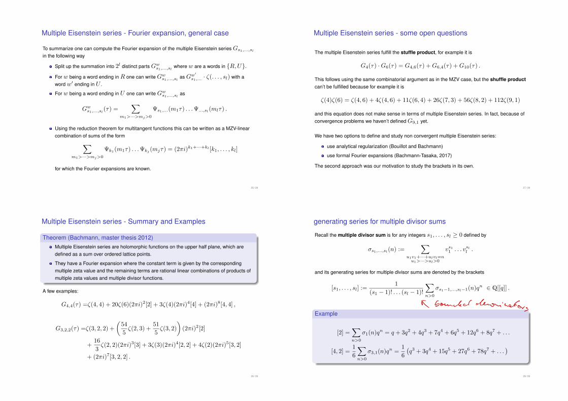
Multiple Eisenstein series - Fourier expansion, general case

To summarize one can compute the Fourier expansion of the multiple Eisenstein series Gs1,...,sl

in the following way

Split up the summation into 2l distinct parts Gw

s1,...,slwhere w are a words in {R,U}.

For w being a word ending in R one can write Gw

s1,...,slas Gw

0

s1,...· ⇣(. . . , s

l

) with aword w0 ending in U .

For w being a word ending in U one can write Gw

s1,...,slas

G

w

s1,...,sl(⌧) =

X

m1>···>mj>0

s1,...(m1

⌧) . . . ...,sl(ml

⌧) .

Using the reduction theorem for multitangent functions this can be written as a MZV-linearcombination of sums of the form

X

m1>···>mj>0

k1(m1

⌧) . . . kj (mj

⌧) = (2⇡i)k1+···+kl [k1

, . . . , k

l

]

for which the Fourier expansions are known.

25 / 39

Multiple Eisenstein series - Summary and Examples

Theorem (Bachmann, master thesis 2012)Multiple Eisenstein series are holomorphic functions on the upper half plane, which aredefined as a sum over ordered lattice points.

They have a Fourier expansion where the constant term is given by the correspondingmultiple zeta value and the remaining terms are rational linear combinations of products ofmultiple zeta values and multiple divisor functions.

A few examples:

G

4,4

(⌧) =⇣(4, 4) + 20⇣(6)(2⇡i)2[2] + 3⇣(4)(2⇡i)4[4] + (2⇡i)8[4, 4] ,

G

3,2,2

(⌧) =⇣(3, 2, 2) +

✓54

5⇣(2, 3) +

51

5⇣(3, 2)

◆(2⇡i)2[2]

+16

3⇣(2, 2)(2⇡i)3[3] + 3⇣(3)(2⇡i)4[2, 2] + 4⇣(2)(2⇡i)5[3, 2]

+ (2⇡i)7[3, 2, 2] .

26 / 39

Multiple Eisenstein series - some open questions

The multiple Eisenstein series fulfill the stuffle product, for example it is

G

4

(⌧) ·G6

(⌧) = G

4,6

(⌧) +G

6,4

(⌧) +G

10

(⌧) .

This follows using the same combinatorial argument as in the MZV case, but the shuffle product

can’t be fulfilled because for example it is

⇣(4)⇣(6) = ⇣(4, 6) + 4⇣(4, 6) + 11⇣(6, 4) + 26⇣(7, 3) + 56⇣(8, 2) + 112⇣(9, 1)

and this equation does not make sense in terms of multiple Eisenstein series. In fact, because ofconvergence problems we haven’t defined G

9,1

yet.

We have two options to define and study non convergent multiple Eisenstein series:

use analytical regularization (Bouillot and Bachmann)

use formal Fourier expansions (Bachmann-Tasaka, 2017)

The second approach was our motivation to study the brackets in its own.

27 / 39

generating series for multiple divisor sums

Recall the multiple divisor sum is for any integers s1

, . . . , s

l

� 0 defined by

�

s1,...,sl(n) :=X

u1v1+···+ulvl=n

u1>···>ul>0

v

s11

. . . v

sll

.

and its generating series for multiple divisor sums are denoted by the brackets

[s1

, . . . , s

l

] :=1

(s1

� 1)! . . . (sl

� 1)!

X

n>0

�

s1�1,...,sl�1

(n)qn 2 Q[[q]] .

Example

[2] =X

n>0

�

1

(n)qn = q + 3q2 + 4q3 + 7q4 + 6q5 + 12q6 + 8q7 + . . .

[4, 2] =1

6

X

n>0

�

3,1

(n)qn =1

6

�q

3 + 3q4 + 15q5 + 27q6 + 78q7 + . . .

�

28 / 39

← bounded denominator,

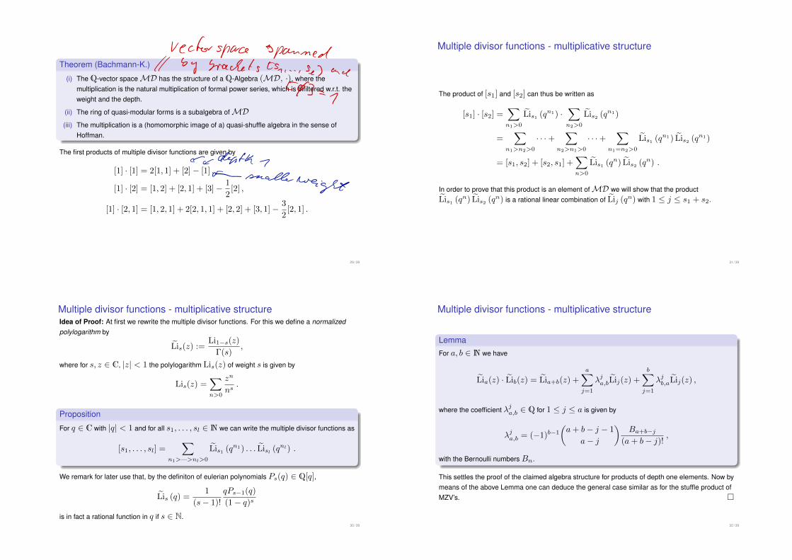
Theorem (Bachmann-K.)

(i) TheQ-vector space MD has the structure of aQ-Algebra (MD, ·), where themultiplication is the natural multiplication of formal power series, which is bifiltered w.r.t. theweight and the depth.

(ii) The ring of quasi-modular forms is a subalgebra of MD(iii) The multiplication is a (homomorphic image of a) quasi-shuffle algebra in the sense of

Hoffman.

The first products of multiple divisor functions are given by

[1] · [1] = 2[1, 1] + [2]� [1] ,

[1] · [2] = [1, 2] + [2, 1] + [3]� 1

2[2] ,

[1] · [2, 1] = [1, 2, 1] + 2[2, 1, 1] + [2, 2] + [3, 1]� 3

2[2, 1] .

29 / 39

greater space spannedby brackets Isn . . -

, Se ) ace

to ]=p

← ← death 7

← smallerweight

Multiple divisor functions - multiplicative structureIdea of Proof: At first we rewrite the multiple divisor functions. For this we define a normalized

polylogarithm by

eLis

(z) :=Li

1�s

(z)

�(s),

where for s, z 2 C, |z| < 1 the polylogarithm Lis

(z) of weight s is given by

Lis

(z) =X

n>0

z

n

n

s

.

Proposition

For q 2 C with |q| < 1 and for all s1

, . . . , s

l

2 N we can write the multiple divisor functions as

[s1

, . . . , s

l

] =X

n1>···>nl>0

eLis1 (q

n1) . . . eLisl (q

nl) .

We remark for later use that, by the definiton of eulerian polynomials Ps

(q) 2 Q[q],

eLis

(q) =1

(s� 1)!

qP

s�1

(q)

(1� q)s

is in fact a rational function in q if s 2 N.30 / 39

Multiple divisor functions - multiplicative structure

The product of [s1

] and [s2

] can thus be written as

[s1

] · [s2

] =X

n1>0

eLis1 (q

n1) ·X

n2>0

eLis2 (q

n1)

=X

n1>n2>0

· · ·+X

n2>n1>0

· · ·+X

n1=n2>0

eLis1 (q

n1) eLis2 (q

n1)

= [s1

, s

2

] + [s2

, s

1

] +X

n>0

eLis1 (q

n) eLis2 (q

n) .

In order to prove that this product is an element of MD we will show that the producteLi

s1 (qn) eLi

s2 (qn) is a rational linear combination of eLi

j

(qn) with 1 j s

1

+ s

2

.

31 / 39

Multiple divisor functions - multiplicative structure

LemmaFor a, b 2 N we have

eLia

(z) · eLib

(z) = eLia+b

(z) +aX

j=1

�

j

a,b

eLij

(z) +bX

j=1

�

j

b,a

eLij

(z) ,

where the coefficient �j

a,b

2 Q for 1 j a is given by

�

j

a,b

= (�1)b�1

✓a+ b� j � 1

a� j

◆B

a+b�j

(a+ b� j)!,

with the Bernoulli numbers Bn

.

This settles the proof of the claimed algebra structure for products of depth one elements. Now bymeans of the above Lemma one can deduce the general case similar as for the stuffle product ofMZV’s. ⇤

32 / 39

Multiple divisor functions - Derivation

Theorem (Bachmann-K.)

The operator d = q

d

dq

is a derivation on MD.

Examples:

d[1] = [3] +1

2[2]� [2, 1] ,

d[2] = [4] + 2[3]� 1

6[2]� 4[3, 1] ,

d[2] = 2[4] + [3] +1

6[2]� 2[2, 2]� 2[3, 1] ,

d[1, 1] = [3, 1] +3

2[2, 1] +

1

2[1, 2] + [1, 3]� 2[2, 1, 1]� [1, 2, 1] .

The second and third equation lead to the first linear relation between multiple divisor functions inweight 4:

[4] = 2[2, 2]� 2[3, 1] + [3]� 1

3[2] .

33 / 39

H

Multiple divisor functions - Connections to MZV

For k 2 N consider the map Zk

: FilWk

(MD) ! R [ {±1} given by

Z

k

(f) = limq!1

(1� q)kf(q) .

Theorem (B.-K., arXiv.NT:1309.3920)(i) For s

1

> 1 and s1

+ · · ·+ s

l

= k it is

Z

k

([s1

, . . . , s

l

]) = ⇣(s1

, . . . , s

l

) .

(ii) If s1

+ · · ·+ s

l

< k then Zk

([s1

, . . . , s

l

]) = 0.

(iii) For any f 2 FilWk�2

(MD) we have Zk

(d(f)) = 0.

(iv) If f 2 FilWk

(MD) is a cusp form for SL2

(Z), then Zk

(f) = 0.

Elements in the kernel of Zk

give rise to relations between MZV. In particular since 0 2 kerZk

,any linear relation between multiple divisor functions in FilW

k

(MD) gives an element in thekernel.

34 / 39

murther , if f ofweight

Er -2

Multiple divisor functions - Connections to MZV

We also rediscover exotic relations related to cusp forms, e.g. the cusp form� = q

Qn>0

(1� q

n)24 can be written as

1

26 · 5 · 691� = 168[5, 7] + 150[7, 5] + 28[9, 3]

+1

1408[2]� 83

14400[4] +

187

6048[6]� 7

120[8]� 5197

691[12] .

Letting Z12

act on both sides one obtains the relation

5197

691⇣(12) = 168⇣(5, 7) + 150⇣(7, 5) + 28⇣(9, 3) .

These type of relations can also be explained via the theory of period polynomials (Gangl,Kaneko, Zagier) or via a motivic interpretation (Pollack, Schneps, Baumard).

35 / 39

Multiple divisor functions - Summary

Multiple divisor functions are formal power series in q with coefficient inQ coming from thecalculation of the Fourier expansion of multiple Eisenstein series.

The space spanned by all multiple divisor functions form an differential algebra whichcontains the algebra of (quasi-) modular forms.

A connection to multiple zeta values is given by the map Zk

whose kernel contains allrelations between multiple zeta values of weight k.

Some questions and open problems:

(i) Is there a modular/geometric/motivic interpretation of the multiple divisor functions ?(ii) Dimensions of the graded parts ? Basis ?(iii) Is there an analogue of the Broadhurst-Kreimer conjecture ? Algebra generators ?(iv) What is the kernel of Z

k

?

36 / 39