Multiple scattering in atmospheric clouds:lidar observations

S. R. Pal and A. 1. Carswell

The contribution of multiple scattering in lidar backscattering from clouds has been investigated using aruby laser at 694 nm. The depolarization of an incident linearly polarized signal is measured with a multi-channel lidar receiver. An analysis is presented whereby this information can be utilized to measure themultiple scattering in clouds in which single scattering retains the incident linear polarization. Experimen-tal data are presented for cumulus clouds and for ground level fog, and the results are compared with somerecent theoretical computations.

Introduction

With the advent of lasers to serve as sources for lidarsystems, great advances have been made in recent yearsin diagnostics of the atmosphere utilizing various lightscattering processes. Most of this work has involvedsingle scattering processes because of the relatively lowdensity of scatterers usually encountered in the atmo-sphere. However in situations of high turbidity suchas those encountered in clouds, fogs, and smoke plumes,the lidar signatures are very difficult to interpret be-cause of the significant contribution of multiple scat-tering to the backscattered signal.

The investigation of multiple scattering in the at-mosphere has received considerable attention for manyyears. However because of the complexity of theproblem, progress in general has been quite slow in thisarea. The availability of large high speed computershas led to the development of a number of numericalcalculation models for multiple scattering situations ofatmospheric interest." Although many of these dealwith the scattering of solar radiation passing througha planetary atmosphere, a number treat the lidar relatedproblems directly.5-1' As a result of these advancesthere are now in existence some calculations that maybe compared with experimental measurements.

Experimentally there have been only a few directlidar investigations of the multiple scattering processesin the atmosphere,'2 -' 5 and there is a great need foradditional measurements of this type. Such mea-surements are, in general, quite difficult to make, notonly because of the inherent complexities of the mul-tiple scattering process itself but also because of the

The authors are with York University, Department of Physics &CRESS, Toronto, Ontario M3J 1P3.

Received 24 November 1975.

spatial and temporal variations of the real atmosphere,particularly in the regions of high turbidity (clouds, fogs,and smoke plumes). In this paper we summarize re-sults of measurements on clouds in which an effort ismade in the data analysis to separate the contributionof multiple scattering in the return signal by making useof the polarization information content of the return.Although a number of simplifying assumptions aremade, it is found that even this rather elementary ap-proach can provide meaningful information about themultiple scattering process and with further refine-ments could provide valuable insight and informationon the basic mechanisms.

It is well known that multiple scattering leads to anappreciable depolarization of an incident linearly po-larized lidar pulse. Thus in situations in which it isknown that the single scattering retains the incidentpolarization in the backscattered signal (Mie scatteringfrom spherical particles), it is possible to separate themultiple scattered signal by using the depolarization asa tracer. In the present study this approach has beenapplied to lidar measurements of low level cumulusclouds which are known to be dominated by sphericalparticle scattering processes.16

The apparatus employed is the York University lidarsystem which is capable of making simultaneous mea-surements of the various Stokes vector components ofthe backscattered signal. All the results presented herewere obtained with the system operating at 694 nm.The transmitter pulselength was 20 nsec, and the beamdivergence was 3 mrad. The receivers had a 7-mradfield of view.

Analysis

When only single scattering occurs the lidar equationfor a linearly polarized transmitted pulse can be writtenas

1990 APPLIED OPTICS / Vol. 15, No. 8 / August 1976

P = (A/R2 )#,r exp(-2r), (1)

where A includes the usual lidar parameters such aspulselength, transmitted power, and area of the receiver.R is the range to the scattering volume.

f= fR fdR

is the attenuation coefficient. fl and j3 are the volumescattering and extinction coefficients.

In a turbid medium the rate of attenuation of a lidarpulse in the presence of multiple scattering is less thanthat for single scattering only because of beam replen-ishment by the near-forward multiple scattered radia-tion. Since some single scattering photon loss is com-pensated for by the presence of multiple scatteringwithin the field of view of the receiver, the attenuationin the lidar equation is therefore reduced by a coefficientTm, and the lidar equation in this case can be written as

P11 = (A/R2 )03 expl-2(r - m)]. (2)

P11 represents the intensity measured in the receiverwith a plolarizer aligned parallel to the transmittedpolarization that includes the multiple scattering con-tribution in this plane. If it is assumed that the mul-tiple scattering is the only source of depolarization inthe medium and that it leads to a complete depolar-ization of the backscattering from the incident linearlypolarized signal, it is possible to separate the multiplescattering contribution. With these assumptions wesee that the single scattered return in the presence ofmultiple scattering is given by P: = P1- PI, where PIis the backscattered intensity observed with the receiverpolarizer oriented in a plane orthogonal to that of thetransmitted polarization. P1 is zero for single back-scattering from spherical particles and only arises fromthe depolarized multiple scattered radiation. UtilizingEqs. (1) and (2), we can write

P11 = Pi exp(2rm) = (Pl - P1 ) exp(2rm). (3)

The coefficient Tm can thus be given by the relation

Tm = i ln[Pii/(Pi - Pi-)]. (4)

A volume scattering coefficient for multiple scattering

A3

m similar to :3 can also be introduced by using the re-lationship that

O3m = (d/dR)(Tm),

1m = (d/dR)['A ln[P11/(P11 - P)]. (5)

Since both P11 and P1 can be measured simultaneouslyas a function of range in a turbid situation, it is possibleto utilize Eqs. (4) and (5) for direct measurements of Tm

and fim.Equation (2) can also be rewritten as

P11 = (A/R2 )32,, expl-2r[1-(Tm/T)]}= (A/R2 3,, exp(-2nT), (6)

where n = 1 - mIT is a parameter similar to the oneintroduced by Platt17 for describing the multiple scattercontribution.

Recent calculations by Kunkel and Weinman18,19

have introduced the multiple scattering in terms of aparameter F defined by the relationship

PT/P1 = exp((2f I3Fdx) = exp(23Px), (7)

where PT is the total backscatter power measured in-cluding multiple scattering, and P, is the backscatterpower arising from single scattering only, without con-sidering the polarization of the transmitted or receivedsignal. F is termed the attenuation correction factor.x is the pulse penetration depth in the turbid mediummeasured from the point of entry to the scattering vol-ume.

On the basis of the assumptions made above it ispossible to express the ratio PT/PI in terms of thequantities P11 and P1 measured by the polarized re-ceivers. This relationship is

PT/P1 = (P11 + PI)/(PHi - PI). (8)

Thus it is possible to express F in terms of the measuredquantities as well by the relationship

P = [1/(2#x)] ln[(P11 + P1)/(P 11 - P * (9)

Equation (9) permits the direct comparison of our ex-perimental values with those calculated using MonteCarlo and approximate analytical techniques byWeinman and Kunkel.

The major question in applying the above analysis ishow well the cross-polarized component represents thetotal multiple scattered signal in the lidar return. Forfully developed multiple scattering, i.e., several scat-tering steps, the assumption of complete depolarizationof the multiple backscattered signal should be valid.However, in the backscattered signal arising from thelower order multiple scattering processes there couldremain a substantial contribution of the incident po-larization. The size of this contribution and its spatialdevelopment within the turbid medium is difficult toascertain. Eloranta10 in his calculations of doublescattering indicates that for a type C-1 cloud20 at analtitude of 1 km the ratio of unpolarized double scatterto polarized double scatter is about 0.5 for a pulse pen-etration depth of 100 m. This contribution would beeven larger if the higher orders of multiple scatteringwere included. The assumption of complete depolar-ization in multiple scattering is also consistent with thework of Bucherl and Werner.14 Obviously the detaileddescription of the polarization characteristics will de-pend on the specific properties of the scattering mediumand on the beamwidth of the receiving optics.

In any event it is clear that the use of the cross-po-larized backscatter component as a measure of themultiple scatter contribution provides a lower limit tothe true amount of multiple scattering and can serve asan extremely useful and readily obtained indicator forfurther studies of such scattering. Additional infor-mation can also be derived by varying the receiver fieldof view as reported by Werner.14 Even here, however,the signal does not relate in a simple way to the observedfield of view, and additional assumptions are required.

August 1976 / Vol. 15, No. 8 / APPLIED OPTICS 1991

I::: /80

/1750

/690L180 0

Fig. 1. Simultaneous record of backscatter intensity in the planeparallel (11) and orthogonal (l) to the plane of polarization of thetransmitted pulse for cumulus clouds in October 1973. The relative

magnitudes of the two signals are arbitrary.

MeasurementsIn this paper we present experimental measurements

of the multiple scattering arising in low lying cumulusclouds and fogs in which it is evident that the dominantscattering is caused by the spherical droplets. Thiseliminates the depolarization contribution arising frombackscattering by nonuniform or jagged particles suchas ice crystals. The data to be presented represent aselection of typical results obtained during the last 2 or3 years with the ruby system. Although the details oflidar signatures from cumulus clouds can vary consid-erably, the general trends indicated by the data pre-sented are typical for this type of turbid scattering.

For the multiple scattering measurements only, tworeceiving channels were required, one with a polarizeraligned parallel to the direction of the transmitted linearpolarization and the other with a polarizer aligned atright angles. The two traces were recorded simulta-neously on a dual beam oscilloscope, and the data werereduced as described in a previous publication.'3

Figure 1 shows two photographs of lidar returns ob-tained from a stratocumulus cloud layer. Each pho-tograph shows a pair of traces indicating the parallel andperpendicular component of the backscattered signal.The two photographs were taken a few minutes apartand illustrate the reasonably stable conditions existingat that time. These curves are typical of those pre-sented in an earlier publication 3 and clearly display theupward shift of the maximum perpendicular signal withrespect to the parallel return.

Using the measured values of the parallel .and per-pendicular signals at each altitude it is possible to plotTm as a function of cloud penetration depth utilizing Eq.(4). This has been done, and the results are shown inFig. 2. In this figure, Tm is plotted as a function of thepenetration depth which is the distance measured fromthe cloud base. In Fig. 2 discrete points are plottedcorresponding to the increments used in digitizing thephotographic records. In fact as the photographs show,a continuous data record is available from cloud baseupward. The scatter of the points at larger penetrationdepths indicates the lower value of the signal to noisein this region.

In Fig. 2 data are shown for pairs of soundings takenon two different dates. Curves (a) and (b) are those of

Fig. 1 and were obtained 3 min apart on a cumulus layerin October 1973, and curves (c) and (d) were obtainedfrom soundings on a similar cloud 3 min apart in Sep-tember 1972. The plots show that the data obtainedover the 3-min intervals exhibit considerable variationbut that the general trend of the plot is retained. Thedifferences between the clouds on the two differentdates are more pronounced. However, for these cu-mulus layers all the curves show a common trend, thatis, that Tm starts at cloud base with a value close to zeroand increases with increasing penetration depth.

For both data sets it is seen that the clouds exhibit afinite distance near cloud base over which Tm has a verylow value. After this region the Tm increases almostlinearly with penetration, with the slope being differenton the two dates. This presence at cloud base of anextremely low value of the depolarization, and hence Tm,is quite characteristic of these low lying cumulus cloudsand would indicate the presence of a dilute layer ofsingle scattering spherical particles. The thickness ofthis layer can vary considerably as is illustrated by thedifferences for the two sets shown in Fig. 2.

In Fig. 3 are shown the oscilloscope photographs fortwo different kinds of cloud layers. On this occasionthere was a layer of scattered cumulus clouds floatingby at an altitude of about 3.5 km, while simultaneouslyat about 10 km there was a layer of cirrus clouds. Fig-ure 3(a) shows the return from the low level layer, and

K-

lbLu~

Lu

/40 A S

0 l

a

/00Q -

a0 0

80 (c0 *d ga. 340~~ asa&

80 . 0 0b)600S0

.4

600a

d 0*° @ - 02 04

Em

Fig. 2. Samples of the variation of rm with pulse penetration fromcloud base. Data (a) and (b) are from Fig. 1 and were obtained 3 minapart from the same strato-cumulus layer in October 1973. Data (c)

and (d) were similarly obtained in September 1972.

1992 APPLIED OPTICS / Vol. 15, No. 8 / August 1976

3550L lIl_

3490

-. ~ ~~~~~~~~~~ I3430~-

3370L/2770

1/270

9770

62700 0

SACKSCArTER INTENSTY

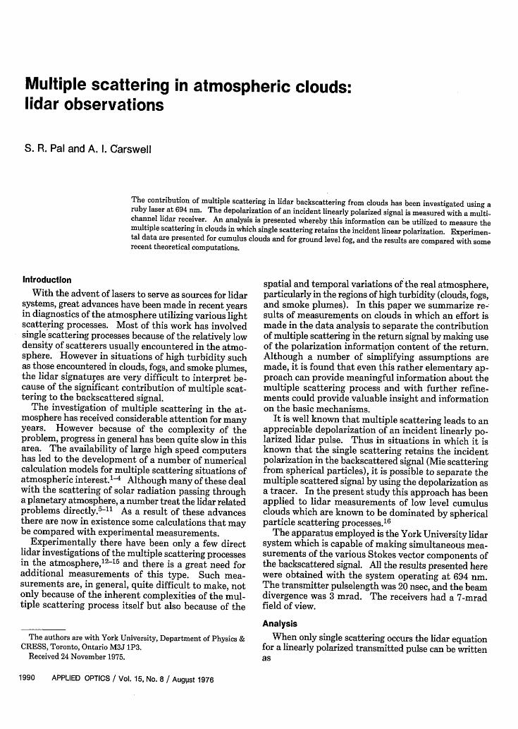
Fig. 3. Simultaneous record of backscatter intensity similar to Fig.1. Trace (a) is for a broken cumulus cloud, and (b) is for a cirrus cloud

above in August 1974.

/20 2000

/00 ) CIRRUS|t dab, {d~~~~~ a ~1,500

4~~~~~~480 X 4 . *1 s

4 *

K0 4 4 0

440 0

Lu I Io *( O AC) 60 4| H CUMULUS /000 8

0 Ads j 00

lo 0.2 0.40

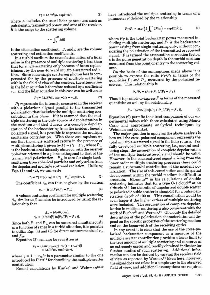
Fig. 4. Tfm variation with penetration depth for thicker cumulusclouds and a cirrus cloud. Data (a) and Nb are from Fig. 3, and data

(c and (d) are two soundings 2 min apart from a thick cumulus layerin May 1973.

Fig. 3(b) shows the return from the cirrus cloud. Thesedata were obtained by recording the cirrus signaturewhen there was no cumulus cloud in the lidar field ofview. The marked differences in the polarizationproperties of the scattering from these different cloudtypes as reported previously 13 is quite evident in thephotographs of Fig. 3. On this occasion the low levelcumulus clouds were appreciably more optically densethan those illustrated in Figs. 1 and 2.

In Fig. 4 are presented data for the curves of Fig. 3along with those obtained on two other occasions fromvery dense cumulus clouds. In this figure we have againplotted r,, as a function of penetration depth. It shouldbe noted that the data for the cirrus cloud are plottedusing the right-hand ordinate scale. For the three cu-mulus clouds plotted in Fig. 4 the trend of rm withpenetration depth is generally similar to that shown inFig. 2 with -rm, increasing from a value of zero at cloud

base. However, in Fig. 4 it is apparent that the valueof Tm as well as its rate of increase with penetrationdepth is considerably greater than that shown in Fig. 2.The behavior for the cirrus cloud is completely differentfrom that of the cumulus clouds. For the cirrus layerthe depolarization increases rapidly at cloud base andremains constant throughout the layer leading to anapparent Tm behavior as shown in Fig. 4. However, inthe cirrus clouds where the particle densities are muchlower than in cumulus and where ice crystals are knownto occur, the analysis outlined above does not apply, andTm in this situation has no simple interpretation (i.e.,the cross-polarized signal does not necessarily arise frommultiple scattering).

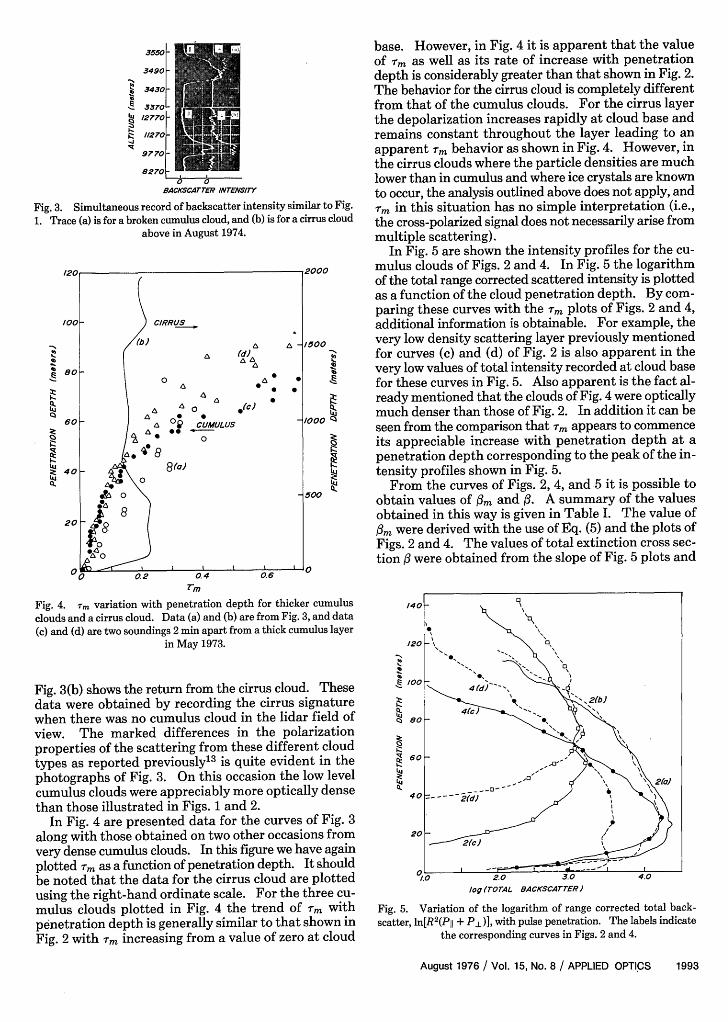
In Fig. 5 are shown the intensity profiles for the cu-mulus clouds of Figs. 2 and 4. In Fig. 5 the logarithmof the total range corrected scattered intensity is plottedas a function of the cloud penetration depth. By com-paring these curves with the rm plots of Figs. 2 and 4,additional information is obtainable. For example, thevery low density scattering layer previously mentionedfor curves (c) and (d) of Fig. 2 is also apparent in thevery low values of total intensity recorded at cloud basefor these curves in Fig. 5. Also apparent is the fact al-ready mentioned that the clouds of Fig. 4 were opticallymuch denser than those of Fig. 2. In addition it can beseen from the comparison that Tm appears to commenceits appreciable increase with penetration depth at apenetration depth corresponding to the peak of the in-tensity profiles shown in Fig. 5.

From the curves of Figs. 2, 4, and 5 it is possible toobtain values of Om and 3. A summary of the valuesobtained in this way is given in Table I. The value of[am were derived with the use of Eq. (5) and the plots ofFigs. 2 and 4. The values of total extinction cross sec-tion 3 were obtained from the slope of Fig. 5 plots and

K

I.

kLr

0!

K

2.0 3.0log (rOAL BACKSCArrER)

Fig. 5. Variation of the logarithm of range corrected total back-scatter, ln[R2 (PII + PI)], with pulse penetration. The labels indicate

the corresponding curves in Figs. 2 and 4.

August 1976 / Vol. 15, No. 8 / APPLIED OPTICS 1993

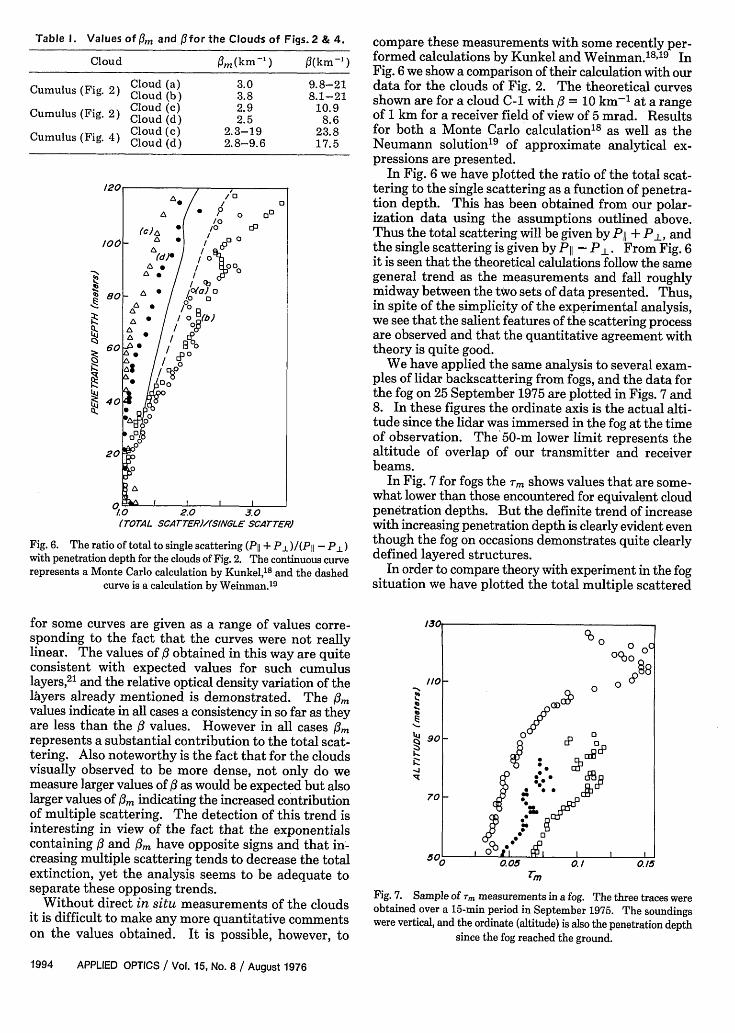
Table I. Values of fam and flfor the Clouds of Figs. 2 & 4.

Cloud Om (km -') 3(km-')

Cumulus (Fig. 2) Cloud (a) 3.8 81-21Cloud () 2.9 810.9

Cumulus (Fig. 2) Cloud (d) 2.9 109

Cumulus (Fig. 4) Cloud (c) 2.3-19 23.8Cloud (d) 2.8-9.6 17.5

I-.

Klb

Lu0.'

o- I XI I I I

/0 2.0 3.0(rOrAL SCA7TER)/(SINGLE SCARTER)

Fig. 6. The ratio of total to single scattering (P11+ PI )I(P11 - P )with penetration depth for the clouds of Fig. 2. The continuous curverepresents a Monte Carlo calculation by Kunkel,18 and the dashed

curve is a calculation by Weinman.1 9

for some curves are given as a range of values corre-sponding to the fact that the curves were not reallylinear. The values of obtained in this way are quiteconsistent with expected values for such cumuluslayers,21 and the relative optical density variation of thelayers already mentioned is demonstrated. The [3mvalues indicate in all cases a consistency in so far as theyare less than the values. However in all cases [3mrepresents a substantial contribution to the total scat-tering. Also noteworthy is the fact that for the cloudsvisually observed to be more dense, not only do wemeasure larger values of as would be expected but alsolarger values of [3m indicating the increased contributionof multiple scattering. The detection of this trend isinteresting in view of the fact that the exponentialscontaining [3 and [3m have opposite signs and that in-creasing multiple scattering tends to decrease the totalextinction, yet the analysis seems to be adequate toseparate these opposing trends.

Without direct in situ measurements of the cloudsit is difficult to make any more quantitative commentson the values obtained. It is possible, however, to

compare these measurements with some recently per-formed calculations by Kunkel and Weinman.18,19 InFig. 6 we show a comparison of their calculation with ourdata for the clouds of Fig. 2. The theoretical curvesshown are for a cloud C-1 with [3 = 10 km'1 at a rangeof 1 km for a receiver field of view of 5 mrad. Resultsfor both a Monte Carlo calculation'8 as well as theNeumann solution19 of approximate analytical ex-pressions are presented.

In Fig. 6 we have plotted the ratio of the total scat-tering to the single scattering as a function of penetra-tion depth. This has been obtained from our polar-ization data using the assumptions outlined above.Thus the total scattering will be given by P11 + Pa, andthe single scattering is given by P11 - P . From Fig. 6it is seen that the theoretical calulations follow the samegeneral trend as the measurements and fall roughlymidway between the two sets of data presented. Thus,in spite of the simplicity of the experimental analysis,we see that the salient features of the scattering processare observed and that the quantitative agreement withtheory is quite good.

We have applied the same analysis to several exam-ples of lidar backscattering from fogs, and the data forthe fog on 25 September 1975 are plotted in Figs. 7 and8. In these figures the ordinate axis is the actual alti-tude since the lidar was immersed in the fog at the timeof observation. The 50-m lower limit represents thealtitude of overlap of our transmitter and receiverbeams.

In Fig. 7 for fogs the m shows values that are some-what lower than those encountered for equivalent cloudpenetration depths. But the definite trend of increasewith increasing penetration depth is clearly evident eventhough the fog on occasions demonstrates quite clearlydefined layered structures.

In order to compare theory with experiment in the fogsituation we have plotted the total multiple scattered

1/0--h

ft

SOl

Lu

K2K1-j

90 F-

70 H

__0

I7 ° 0I 0 *

0.05Em

V. 0 0C

000

00d

1 1

0./ 0.15

Fig. 7. Sample of rm measurements in a fog. The three traces wereobtained over a 15-min period in September 1975. The soundingswere vertical, and the ordinate (altitude) is also the penetration depth

since the fog reached the ground.

1994 APPLIED OPTICS / Vol. 15, No. 8 / August 1976

I.

^ r] __

_ ._ r

070

A

0~~~~~~

0 0./ 0.2 0.(TOTAL MULIPLE scArrER)I(slNeLE SCATT ER)

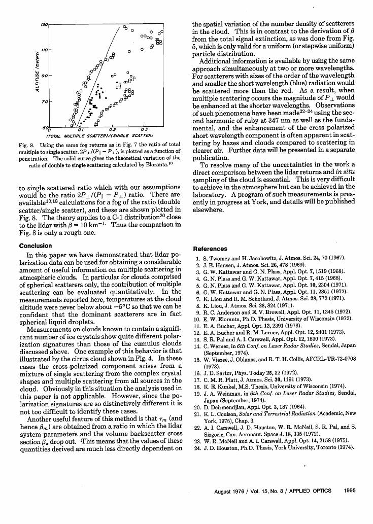
Fig. 8. Using the same fog returns as in Fig. 7 the ratio of total

multiple to single scatter, 2P I (P11 - P-), is plotted as a function ofpenetration. The solid curve gives the theoretical variation of the

ratio of double to single scattering calculated by Eloranta.10

to single scattered ratio which with our assumptionswould be the ratio 2PlAP- nP) ratio. There areavailable 108 calculations for a fog of the ratio (doublescatter/single scatter), and these are shown plotted inFig. 8. The theory applies to a C-1 distribution20 closeto the lidar with r 10 km1 Thus the comparison inFig. 8 is only a rough one.

Conclusion

In this paper we have demonstrated that lidar po-larization data can be used for obtaining a considerableamount of useful information on multiple scattering inatmospheric clouds. In particular for clouds comprisedof spherical scatterers only, the contribution of multiplescattering can be evaluated quantitatively. In themeasurements reported here, temperatures at the cloudaltitude were never below about -5 0 C so that we can beconfident that the dominant scatterers are in factspherical liquid droplets.

Measurements on clouds known to contain a signifi-cant number of ice crystals show quite different polar-ization signatures than those of the cumulus cloudsdiscussed above. One example of this behavior is thatillustrated by the cirrus cloud shown in Fig. 4. In thesecases the cross-polarized component arises from amixture of single scattering from the complex crystalshapes and multiple scattering from all sources in thecloud. Obviously in this situation the analysis used inthis paper is not applicable. However, since the po-larization signatures are so distinctively different it isnot too difficult to identify these cases.

Another useful feature of this method is that Tm (andhence [3m) are obtained from a ratio in which the lidarsystem parameters and the volume backscatter crosssection 0, drop out. -This means that the values of thesequantities derived are much less directly dependent on

the spatial variation of the number density of scatterersin the cloud. This is in contrast to the derivation of [from the total signal extinction, as was done from Fig.5, which is only valid for a uniform (or stepwise uniform)particle distribution.

Additional information is available by using the sameapproach simultaneously at two or more wavelengths.For scatterers with sizes of the order of the wavelengthand smaller the short wavelength (blue) radiation wouldbe scattered more than the red. As a result, whenmultiple scattering occurs the magnitude of P 1 wouldbe enhanced at the shorter wavelengths. Observationsof such phenomena have been made22 -24 using the sec-ond harmonic of ruby at 347 nm as well as the funda-mental, and the enhancement of the cross polarizedshort wavelength component is often apparent in scat-tering by hazes and clouds compared to scattering inclearer air. Further data will be presented in a separatepublication.

To resolve many of the uncertainties in the work adirect comparison between the lidar returns and in situsampling of the cloud is essential. This is very difficultto achieve in the atmosphere but can be achieved in thelaboratory. A program of such measurements is pres-ently in progress at York, and details will be publishedelsewhere.

References

1. S. Twomey and H. Jacobowitz, J. Atmos. Sci. 24, 70 (1967).

2. J. E. Hansen, J. Atmos. Sci. 26, 478 (1969).3. G. W. Kattawar and G. N. Plass, Appl. Opt. 7, 1519 (1968).

4. G. N. Plass and G. W. Kattawar, Appl. Opt. 7, 415 (1968).

5. G. N. Plass and G. W. Kattawar, Appl. Opt. 10, 2304 (1971).6. G. W. Kattawar and G. N. Plass, Appl. Opt. 11, 2851 (1972).

7. K. Liou and R. M. Schotland, J. Atmos. Sci. 28, 772 (1971).

8. K. Liou, J. Atmos. Sci. 28, 824 (1971).9. R. C. Anderson and E. V. Browell, Appl. Opt. 11, 1345 (1972).

10. E. W. Eloranta, Ph.D. Thesis, University of Wisconsin (1972).

11. E. A. Bucher, Appl. Opt. 12, 2391 (1973).12. E. A. Bucher and R. M. Lerner, Appl. Opt. 12, 2401 (1973).

13. S. R. Pal and A. I. Carswell, Appl. Opt. 12, 1530 (1973).14. C. Werner, in 6th Conf. on Laser Radar Studies, Sendai, Japan

(September, 1974).15. W. Viezee, J. Oblanas, and R. T. H. Collis, AFCRL-TR-73-0708

(1973).16. J. D. Sartor, Phys. Today 25, 32 (1972).17. C. M. R. Platt, J. Atmos. Sci. 30, 1191 (1973).18. K. E. Kunkel, M.S. Thesis, University of Wisconsin (1974).

19. J. A. Weinman, in 6th Conf. on Laser Radar Studies, Sendai,Japan (September, 1974).

20. D. Deirmendjian, Appl. Opt. 3, 187 (1964).21. K. L. Coulson, Solar and Terrestrial Radiation (Academic, New

York, 1975), Chap. 3.22. A. I. Carswell, J. D. Houston, W. R. McNeil, S. R. Pal, and S.

Sizgoric, Can. Aeronaut. Space J. 18, 335 (1972).23. W. R. McNeil and A. I. Carswell, Appl. Opt. 14, 2158 (1975).

24. J. D. Houston, Ph.D. Thesis, York University, Toronto (1974).

August 1976 / Vol. 15, No. 8 / APPLIED OPTICS 1995