HAL Id: hal-01397150https://hal.inria.fr/hal-01397150

Submitted on 15 Nov 2016

HAL is a multi-disciplinary open accessarchive for the deposit and dissemination of sci-entific research documents, whether they are pub-lished or not. The documents may come fromteaching and research institutions in France orabroad, or from public or private research centers.

L’archive ouverte pluridisciplinaire HAL, estdestinée au dépôt et à la diffusion de documentsscientifiques de niveau recherche, publiés ou non,émanant des établissements d’enseignement et derecherche français ou étrangers, des laboratoirespublics ou privés.

Multiple comparative metagenomics using multiset k-mer counting

Gaëtan Benoit, Pierre Peterlongo, Mahendra Mariadassou, Erwan Drezen,Sophie Schbath, Dominique Lavenier, Claire Lemaitre

To cite this version:Gaëtan Benoit, Pierre Peterlongo, Mahendra Mariadassou, Erwan Drezen, Sophie Schbath, et al..Multiple comparative metagenomics using multiset k -mer counting. PeerJ Computer Science, PeerJ,2016, 2, �10.7717/peerj-cs.94�. �hal-01397150�

Multiple comparative metagenomics using multisetk-mer counting

Gaetan Benoit1,*, Pierre Peterlongo1, Mahendra Mariadassou3, ErwanDrezen1,4, Sophie Schbath3, Dominique Lavenier1, Claire Lemaitre1

1 INRIA/IRISA, Genscale team, UMR6074 IRISACNRS/INRIA/Universite de Rennes 1, Campus de Beaulieu, 35042,Rennes, France3 MaIAGE, INRA, Universite Paris-Saclay, 78350, Jouy-en-Josas,France4 CHU Pontchaillou, 35000, Rennes, France

* E-mail: gaetan.benoit@inria.fr

Abstract

Background. Large scale metagenomic projects aim to extract biodiversityknowledge between different environmental conditions. Current methods forcomparing microbial communities face important limitations. Those based ontaxonomical or functional assignation rely on a small subset of the sequencesthat can be associated to known organisms. On the other hand, de novomethods, that compare the whole sets of sequences, either do not scale up onambitious metagenomic projects or do not provide precise and exhaustiveresults.Methods. These limitations motivated the development of a new de novometagenomic comparative method, called Simka. This method computes a largecollection of standard ecological distances by replacing species counts by k-mercounts. Simka scales-up today’s metagenomic projects thanks to a new parallelk-mer counting strategy on multiple datasets.Results. Experiments on public Human Microbiome Project datasetsdemonstrate that Simka captures the essential underlying biological structure.Simka was able to compute in a few hours both qualitative and quantitativeecological distances on hundreds of metagenomic samples (690 samples, 32billions of reads). We also demonstrate that analyzing metagenomes at thek-mer level is highly correlated with extremely precise de novo comparisontechniques which rely on all-versus-all sequences alignment strategy or whichare based on taxonomic profiling.

1

Introduction 1

It is estimated that only a fraction of 10−24 to 10−22 of the total DNA on earth 2

has been sequenced (Nature Rev. Microbiol. editorial, 2011). In large scale 3

metagenomics studies such as Tara Oceans (Karsenti et al., 2011) most of the 4

sequenced data comes from unknown organisms and their short reads assembly 5

remains an inaccessible task (see for instance results from the CAMI 6

challenge http://cami-challenge.org/). When precise taxonomic assignation 7

is not feasible, microbial ecosystems can nevertheless be compared on the basis 8

of their diversity, inferred from metagenomic read sets. In this framework, the 9

beta-diversity, introduced in (Whittaker, 1960), measures the dissimilarities 10

between communities in terms of species composition. Such compositions may 11

be approximated by sequencing marker genes, such as the rRNA 16S in bacterial 12

communities (Liles et al., 2003), and clustering the sequences into Operational 13

Taxonomic Units (OTU) or working species. However, marker genes surveys 14

suffer from amplification and primer bias (Cai et al., 2013) and therefore may 15

not capture the whole microbial diversity of a sample. Furthermore, even within 16

the captured diversity, the marker may not be informative enough to 17

discriminate between sub-species or even species strains (Piganeau et al., 2011). 18

Finally, this approach is impractical for whole metagenomic sets for at least two 19

reasons: clustering reads into putative species is computationally costly and 20

leaves out a large fraction of the reads (Nielsen et al., 2014). 21

In this context, it is more practical to ditch species composition altogether 22

and compare microbial communities using directly the sequence content of 23

metagenomic read sets. This has first been performed by using Blast (Altschul 24

et al., 1990) for comparing read content (Yooseph et al., 2007). This approach 25

was successful but can not scale up to large studies made up of dozens or 26

hundreds of large read sets, such as those generated from Illumina sequencers. 27

In 2012, the Compareads method (Maillet et al., 2012) was proposed. The 28

method compares the whole sequence content of two read sets. It introduced a 29

rough approximation of read similarity based on the number of shared words of 30

length k (k-mer, with k typically around 30) and used it for providing so defined 31

similar reads between read sets. The number of similar reads was then used for 32

computing a Jaccard distance between pairs of read sets. Commet (Maillet 33

et al., 2014) is an extended version of Compareads. It better handles the 34

comparison of large read sets and provides a read sub-set representation that 35

facilitates result analyses and reduces the disk footprint. Seth et al. (2014) used 36

the notion of shared k-mers between samples for estimating dataset similarities. 37

This is a slightly different problem as this was used for retrieving from an 38

indexed database, samples similar to a query sample. More recently, two 39

additional methods were developed to represent a metagenome by a feature 40

vector that is then used to compute pairwise similarity matrices between 41

multiple samples. For both methods, features are based on the k-mer 42

composition of samples, but with a feature representing more than one k-mer 43

and using only a subset of k-mers to reduce the dimension (Ulyantsev et al., 44

2016; Ondov et al., 2016). However, the approaches for k-mer grouping and 45

2

sub-sampling are radically different. In MetaFast (Ulyantsev et al., 2016), the 46

subset of k-mers is obtained by post-processing de novo assemblies performed 47

for each metagenome. A feature represents then a set of k-mers belonging to a 48

same assembly graph “component”. The relative abundance of such component 49

in each sample is then used to compute the Bray-Curtis dissimilarity measure. 50

In Mash (Ondov et al., 2016) a sub-sampling of the k-mers is performed using 51

the MinHash (Broder, 1997) approach (keeping by default 1,000 k-mers per 52

sample). The method outputs then a Jaccard index of the presence-absence of 53

such k-mers in two samples. 54

All these reference-free methods share the use of k-mers as the fundamental 55

unit used for comparing samples. Actually, k-mers are a natural unit for 56

comparing communities: (1) sufficiently long k-mers are usually specific of a 57

genome (Fofanov et al., 2004), (2) k-mer frequency is linearly related to 58

genome’s abundance (Wu and Ye, 2011), (3) k-mer aggregates organisms with 59

very similar k-mer composition (e.g. related strains from the same bacterial 60

species) without need for a classification of those organisms (Teeling et al., 61

2004). Dubinkina et al. (2016) conducted an extensive comparison between 62

k-mer-based distances and taxonomic ones (ie. based on taxonomic assignation 63

against a reference database) for several large scale metagenomic projects. They 64

demonstrate that k-mer-based distances are well correlated to taxonomic ones, 65

and are therefore accurate enough to recover known biological structure, but 66

also to uncover previously unknown biological features that were missed by 67

reference-based approaches due to incompleteness of reference databases. 68

Importantly, the greater k, the more correlated these taxonomic and 69

k-mer-based distances seem to be. However, the study is limited to values of k 70

lower than 11 for computational reasons and the correlation for large values of k 71

still needs to be evaluated. 72

Even if Commet and MetaFast approaches were designed to scale-up to large 73

metagenomic read sets, their use on data generated by large scale projects is 74

turning into a bottleneck in terms of time and/or memory requirements. By 75

contrast, Mash outperforms by far all other methods in terms of computational 76

resource usage. However, this frugality comes at the expense of result quality 77

and precision: the output distances and Jaccard indexes do not take into 78

account relative abundance information and are not computed exactly due to 79

k-mer sub-sampling. 80

In this paper, we present Simka. Simka compares N metagenomic datasets 81

based on their k-mers counts. It computes a large collection of distances 82

classically used in ecology to compare communities. Computation is performed 83

by replacing species counts by k-mer counts, for a large range of kmer sizes, 84

including large ones (up to 30). Simka is, to our knowledge, the first method 85

able to rapidly compute a full range of distances enabling the comparison of any 86

number of datasets. This is performed by processing data on-the-fly (i.e. 87

without storage of large temporary results). With the exception of Mash that is, 88

thanks to sub-sampling, approximately two to five time faster, Simka 89

outperforms state-of-the-art read comparison methods in terms of computational 90

needs. For instance, Simka ran on 690 samples from the Human Microbiome 91

3

Project (HMP) (Human Microbiome Project Consortium, 2012a) (totalling 32 92

billion reads) in less than 10 hours and using no more than 70 GB RAM. 93

The contributions of this manuscript are three-fold. First we propose a new 94

method for efficiently counting k-mers from a large number of metagenomic 95

samples. The usefulness of such counting is not limited to comparative 96

metagenomics and may have applications in many other fields. Second, we show 97

how to derive a large number of ecological distances from k-mer counts. And 98

third, we show on real datasets that k-mer-based distances are highly correlated 99

to taxonomic distances: they therefore capture the same underlying structure 100

and lead to the same conclusions. 101

Materials and Methods 102

The proposed algorithm enables to compute dissimilarity measures between 103

read sets. In the following, in order to simplify the reading, we use the term 104

“distance” to refer to this measure. 105

Overview 106

Given N metagenomic datasets, denoted as S1, S2, Si, ...SN , the objective is to 107

provide a N ×N distance matrix D where Di,j represents an ecological distance 108

between datasets Si and Sj . Such possible distances are listed in Table 1. The 109

computation of the distance matrix can be theoretically decomposed into two 110

distinct steps: 111

1. k-mer count. Each dataset is represented as a set of discriminant 112

features, in our case, k-mer counts. More precisely, a k-mer count matrix 113

KC of size W ×N is computed. W is the number of distinct k-mer 114

among all the datasets. KCi,j represents the number of times a k-mer i is 115

present in the dataset Sj . 116

2. distance computation. Based on the k-mer count information, the 117

distance matrix D is computed. Actually, many ecological distances (cf 118

Table 1) can be derived from matrix KC when replacing species counts by 119

k-mer counts. 120

Actually, Simka does not require to have the full KC matrix to start the 121

distance computation. But for sake of simplicity, we will first consider this 122

matrix to be available. 123

The k-mer count step splits all the reads of the datasets into k-mers and 124

performs a global count. This can be done by counting individually k-mers in 125

each dataset, then merging the overall k-mer counts. The output is the matrix 126

KC (of size W ×N). Efficient algorithms, such as KMC2 (Deorowicz et al., 127

2015), have recently been developed to count all the occurrences of distinct 128

k-mers in a read dataset, allowing the computation to be executed in a 129

reasonable amount of time and memory even on very large datasets. However, 130

4

the main drawback of this approach is the huge main memory space it requires 131

which is computed as follow: MemKC = Ws ∗ (8 + 4N) bytes, with Ws the 132

number of distinct k-mers, N the number of samples, and 8 and 4 the number 133

of bytes required to store respectively 31-mers and a k-mer count. For example, 134

experiments on the HMP (Human Microbiome Project Consortium, 2012a) 135

datasets (690 datasets containing on average 45 millions of reads each) would 136

require a storage space of 260TB for the matrix KC. 137

However, a careful look at the definition of ecological distances (Table 1) 138

shows that, up to some final transformation, they are all additive over the 139

k-mers. Independent contributions to the distance can thus be computed in 140

parallel from disjoint sets of k-mers and aggregated later on to construct the 141

final distance matrix. Furthermore, each independent contribution can itself be 142

constructed in an iterative way by receiving lines of the KC matrix, called 143

abundance vectors, one at a time. The abundance vector of a specific k-mer 144

simply consists of its N counts in the N datasets. 145

To sum up, instead of computing the complete k-mer count matrix KC, the 146

alternative computation scheme we propose is to generate successive abundance 147

vectors from which independent contributions to the distances can be iteratively 148

updated in parallel. The great advantage is that the huge k-mer count matrix 149

KC does not need to be stored anymore. However, this approach requires a new 150

strategy to generate abundance vectors. We propose and describe below a new 151

efficient multiset k-mer counting algorithm (called MKC) that can be highly 152

parallelized on large computing resources infrastructures. As illustrated Fig. 1, 153

Simka uses abundance vectors generated by MKC for computing ecological 154

distances. 155

S1   S2   …   SN  

S1   0   0.2   …   0.1  

S2   0.2   0   …   0.4  

…   …   …   …   …  

SN   0.1   0.4   …   0  

Read  set  S1  

Read  set  S2  

Read  set  SN  

Accumulate  contribu:ons  and  compute  final  distance  matrix  

…  Generate  abundance  vectors  

Update  par:al  contribu:on  to  the  distance  

Update  par:al  contribu:on  to  the  distance  

Update  par:al  contribu:on  to  the  distance  

Update  par:al  contribu:on  to  the  distance  

…  

Figure 1. Simka strategy. The first step takes as input N datasets and generatesmultiple streams of abundance vector from disjoint sets of k-mers. The abundancevector of a k-mer consists of its N counts in the N datasets. These abundance vectorsare taken as input by the second step to iteratively update independent contributionsto the ecological distance in parallel. Once an abundance vector has been processed,there is no need to keep it on record. The final step aggregates each contribution andcomputes the final distance matrix.

5

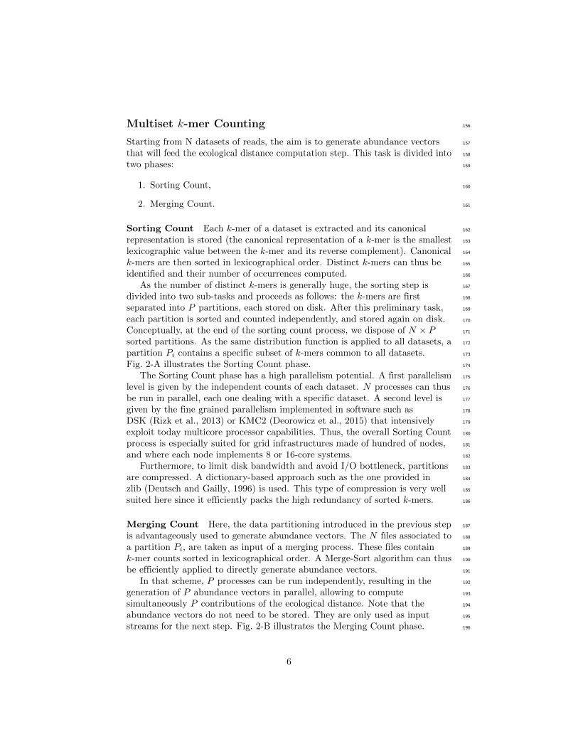
Multiset k-mer Counting 156

Starting from N datasets of reads, the aim is to generate abundance vectors 157

that will feed the ecological distance computation step. This task is divided into 158

two phases: 159

1. Sorting Count, 160

2. Merging Count. 161

Sorting Count Each k-mer of a dataset is extracted and its canonical 162

representation is stored (the canonical representation of a k-mer is the smallest 163

lexicographic value between the k-mer and its reverse complement). Canonical 164

k-mers are then sorted in lexicographical order. Distinct k-mers can thus be 165

identified and their number of occurrences computed. 166

As the number of distinct k-mers is generally huge, the sorting step is 167

divided into two sub-tasks and proceeds as follows: the k-mers are first 168

separated into P partitions, each stored on disk. After this preliminary task, 169

each partition is sorted and counted independently, and stored again on disk. 170

Conceptually, at the end of the sorting count process, we dispose of N × P 171

sorted partitions. As the same distribution function is applied to all datasets, a 172

partition Pi contains a specific subset of k-mers common to all datasets. 173

Fig. 2-A illustrates the Sorting Count phase. 174

The Sorting Count phase has a high parallelism potential. A first parallelism 175

level is given by the independent counts of each dataset. N processes can thus 176

be run in parallel, each one dealing with a specific dataset. A second level is 177

given by the fine grained parallelism implemented in software such as 178

DSK (Rizk et al., 2013) or KMC2 (Deorowicz et al., 2015) that intensively 179

exploit today multicore processor capabilities. Thus, the overall Sorting Count 180

process is especially suited for grid infrastructures made of hundred of nodes, 181

and where each node implements 8 or 16-core systems. 182

Furthermore, to limit disk bandwidth and avoid I/O bottleneck, partitions 183

are compressed. A dictionary-based approach such as the one provided in 184

zlib (Deutsch and Gailly, 1996) is used. This type of compression is very well 185

suited here since it efficiently packs the high redundancy of sorted k-mers. 186

Merging Count Here, the data partitioning introduced in the previous step 187

is advantageously used to generate abundance vectors. The N files associated to 188

a partition Pi, are taken as input of a merging process. These files contain 189

k-mer counts sorted in lexicographical order. A Merge-Sort algorithm can thus 190

be efficiently applied to directly generate abundance vectors. 191

In that scheme, P processes can be run independently, resulting in the 192

generation of P abundance vectors in parallel, allowing to compute 193

simultaneously P contributions of the ecological distance. Note that the 194

abundance vectors do not need to be stored. They are only used as input 195

streams for the next step. Fig. 2-B illustrates the Merging Count phase. 196

6

Read  set  S1  

Read  Set  S2  

Read  set  SN  

CAT 1

ATC 4

AAG 2TTA 4

AAG 8GGC 1

GGC 9TTA 1

ACG 4TTG 2

ATC 8

ACG 1

ATC 2CGG 4

S1 S2 SNACG 0 4 1

P  par33o

ns  

CAG 7 CAG 3CAG 1GAC 6

(A)  Sort  and  Count  k-­‐mers  

(B)  Merge  k-­‐mer  counts  

S1 S2 SNCAT 1 0 0

S1 S2 SNTTG 0 2 0

S1 S2 SNATC 4 8 2

S1 S2 SNCGG 0 0 4

S1 S2 SNAAG 2 8 0

S1 S2 SNGGC 0 1 9

S1 S2 SNTTA 4 0 1

S1 S2 SNCAG 7 3 1

S1 S2 SNGAC 0 0 6

Streams  of  abundance  vectors  

Figure 2. Multiset k-mer Counting strategy with k=3. (A) The sortingcounting process, represented by a blue arrow, counts datasets independently. Eachprocess outputs a column of P partitions (red squares) containing sorted k-mer counts.(B) The merging count process, represented by a green arrow, merges a row of Npartitions. It outputs abundance vectors, represented in green, to feed the ecologicaldistance computation process.

k-mer abundance filter Distinct k-mers with very low abundance usually 197

come from sequencing errors. As a matter of fact, a single sequencing error 198

creates up to k erroneous distinct k-mers. Filtering out these k-mers speeds-up 199

the Simka process, as it greatly reduces the overall number of distinct k-mers, 200

but may also impact the content of the distance matrix. This point is evaluated 201

and discussed in the result section. 202

This filter is activated during the count process. Only k-mers whose 203

abundance is equal to or greater than a given abundance threshold are kept. By 204

default the threshold is set to 2. The k-mers that pass the filter are called “solid 205

k-mers”. 206

Ecological distance computation 207

Simka computes a collection of distances for all pairs of datasets. As detailed in 208

the previous section, abundance vectors are used as input data. For the sake of 209

simplicity, we first explain the computations of the Bray-Curtis distance. All 210

other distances, presented later on, can be computed in the same way, with only 211

small adaptations. 212

7

Computing the Bray-Curtis distance The Bray–Curtis distance is givenby the following equation:

BrayCurtisAb(Si, Sj) = 1− 2

∑w∈Si∩Sj

min(NSi(w), NSj

(w))∑w∈Si

NSi(w) +∑

w∈SjNSj (w)

(1)

where w is a k-mer and NSi(w) is the abundance of w in the dataset Si. We 213

consider here that w ∈ Si ∩ Sj if NSi(w) > 0 and NSj (w) > 0. 214

The equation involves marginal (or dataset specific) terms (i.e. 215∑w∈Si

NSi(w) is the total amount of k-mers in dataset Si) acting as 216

normalizing constants and crossed terms that capture the (dis)similarity 217

between datasets (i.e.∑

w∈Si∩Sjmin(NSi

(w), NSj(w)) is the total amount of 218

k-mers in the intersection of the datasets Si and Sj). Marginal and crossed 219

terms are then combined to compute the final distance. 220

Algorithm 1 shows that it is straightforward to compute the distance matrix 221

between N datasets from the abundance vectors. Inputs of this algorithm are 222

provided by the Multiple k-mer Counting algorithm (MKC). These are the P 223

streams of abundance vectors and the marginal terms of the distance, i.e. the 224

number of k-mers in each dataset, determined during the first step of the MKC 225

which counts the k-mers. 226

A matrix, denoted M∩, of dimension N ×N is initialized (step 1) to record 227

the final value of the crossed terms of each pair of datasets. P independent 228

processes are run (step 2) to compute P partial crossed term matrices, denoted 229

M∩part (step 3), in parallel. Each process iterates over its abundance vector 230

stream (step 4). For each abundance vector, we loop over each possible pair of 231

datasets (steps 5-6). The matrix M∩part is updated (step 8) if the k-mer is 232

shared, meaning that it has positive abundance in both datasets Si and Sj 233

(step 7). Since a distance matrix is symmetric with null diagonal, we limit the 234

computation to the upper triangular part of the matrix M∩part. The current 235

abundance vector is then released. Each process writes its matrix M∩part on the 236

disk when its stream is done (step 9). 237

When all streams are done, the algorithm reads each written M∩part and 238

accumulates it to M∩ (step 10-11). The last loop (steps 13 to 16) computes the 239

Bray-Curtis distance for each pair of datasets and fills the distance matrix 240

reported by Simka. 241

The amount of abundance vectors streamed by the MKC is equal to Ws, 242

which is also the total amount of distinct solid k-mers in the N datasets. This 243

algorithm has thus a time complexity of O(Ws ×N2). 244

Other ecological distances The distance introduced in Eq. 1 is a singleexample of ecological distance. There exists numerous other ecological distancesthat can be broadly classified into two categories (see Legendre and De Caceres(2013) for a finer classification): distances based on presence-absence data(hereafter called qualitative) and distances based on proper abundance data(hereafter called quantitative). Qualitative distances are more sensitive tofactors that affect presence-absence of organisms (such as pH, salinity, depth,

8

Algorithm 1: Compute the Bray-Curtis distance (equation 1) between Ndatasets

Input:- Vs: vector of size P representing the abundance vector streams- V∪: vector of size N containing the number of k-mers in each datasetOutput: a distance matrix Dist

1 M∩ ← empty square matrix of size N // number of k-mers in each datasetintersection

2 In parallel: foreach abundance vector stream S in Vs do3 M∩part ← empty squared matrix of size N // part of M∩4 foreach abundance vector v in S do5 for i← 0 to N − 1 do6 for j ← i + 1 to N − 1 do7 if v[i] > 0 and v[j] > 0 then8 M∩part[i, j] ← M∩part[i, j] + min(v[i], v[j])

9 Write M∩part to disk

10 foreach each written matrix M∩part do11 M∩ ← M∩ + M∩part

12 Dist ← empty squared matrix of size N // final distance matrix13 for i← 0 to N − 1 do14 for j ← i + 1 to N − 1 do15 Dist[i, j] = 1− 2 ∗M∩[i, j] / (V∪[i] + V∪[j])16 Dist[j, i] = 1− 2 ∗M∩[i, j] / (V∪[i] + V∪[j])

17 return Dist

humidity, absence of light, etc) and therefore useful to study bioregions.Quantitative distances focus on factors that affect relative changes (seasonalchanges, nutrient availability, concentration of oxygen, depth, diet, disease, etc)and are therefore useful to monitor communities over time or along anenvironmental gradient. Note that some factors, such as pH, are likely to affectboth presence-absence (for large changes in pH) and relative abundances (forsmall changes in pH). Algorithmically, most ecological distances, including mostof those mentioned in Legendre and De Caceres (2013), can be expressed fortwo datasets Si and Sj as:

Distance(Si, Sj) = g

∑w∈Si∪Sj

f(NSi

(w), NSj(w), CSi

, CSj

) (2)

where g and f are simple functions, and CSiis a marginal (i.e. dataset-specific) 245

term of dataset Si, usually of size 1 (i.e. a scalar). In most distances, CSi is 246

simply the total number of k-mers in Si. By contrast, the value of f corresponds 247

9

to crossed terms and requires knowledge of both NSi(w) and NSj (w) (and 248

potentially CSi and CSj as well). For instance, for the abundance-based 249

Bray-Curtis distance of Eq. 1, we have CSi=∑

w∈SiNSi

(w), g(x) = 1− 2x and 250

f(x, y,X, Y ) = min(x, y)/(X + Y ). Those distances can be computed in a 251

single pass over the data using a slightly modified variant of Algorithm 1. The 252

marginal terms CSiare computed during the first step of the MKC which counts 253

the k-mers of each dataset. The crossed terms involving f are computed and 254

summed in steps 7-8 (but exact instructions depend on the nature of f). Finally, 255

the actual distances are computed in steps 15-16 and depend on both f and g. 256

Qualitative distances form a special case of ecological distances: they can all 257

be expressed in terms of quantities a, b and c where a is the number of distinct 258

k-mers shared between datasets Si and Sj , b is the number of distinct k-mers 259

specific to dataset Si and c is the number of distinct k-mers specific to dataset 260

Sj . Those distances easily fit in the previous framework as 261

a =∑

w∈Si∩Sj1{NSi

(w)NSj(w)>0}, CSi

=∑

w∈Si1{NSi

(w)>0} = a + b and 262

similarly CSj= a + c. Therefore, a is a crossed term and b and c can be 263

deduced from a and the marginal terms. 264

In the same vein, Chao et al. (2006) introduced variations of 265

presence-absence distances incorporating abundance information to account for 266

unobserved species. The main idea is to replace ”hard” quantities such as 267

a/(a + b), the fraction of distinct k-mers from Si shared with Sj , by 268

probabilistic ”soft” ones: here the probability U ∈ [0, 1] that a k-mer from Si is 269

also found in Sj . Similarly, the ”hard” fraction a/(a+ c) of distinct k-mers from 270

Sj shared with Si is replaced by the ”soft” probability V that a k-mer from Sj 271

is also found in Si. U and V play the same role as a, b and c do in qualitative 272

distances and are sufficient to compute the variants named AB-Jaccard, 273

AB-Ochiai and AB-Sorensen. However and unlike the quantities a, b c, which 274

can be observed from the data, U and V are not known in practice and must be 275

estimated from the data. Chao et al. (2006) proposed several estimates for U 276

and V . The most elaborate ones attempt to correct for differences in sampling 277

depths and unobserved species by considering the complete k-mer counts vector 278

of a sample. Those estimates are unfortunately untractable in our case as we 279

stream only a few k-mer counts at a time. Instead we resort to the simplest 280

estimates presented in Chao et al. (2006), which lend themselves well to the 281

additive and distributed nature of Simka: U = YSiSj/CSi

and V = YSjSi/CSj

282

where YSiSj =∑

w∈Si∩SjNSi(w)1{NSj

(w)>0} and CSi =∑

w∈SiNSi(w). Note 283

that YSiSj corresponds to crossed terms and is asymmetric, i.e. YSiSj 6= YSjSi . 284

Intuitively, U is the fraction of k-mers (not distinct anymore) from Si also 285

found in Sj and therefore gives more weights to abundant k-mers that its 286

qualitative counterpart a/(a + b). 287

Table 1 gives the definitions of the collection of distances computed by 288

Simka while replacing species counts by k-mer counts. These are qualitative, 289

quantitative and abundance-based variants of qualitative ecological distances. 290

The table also provides their expression in terms of Ci, f and g, adopting the 291

notations of Eq. 2. 292

10

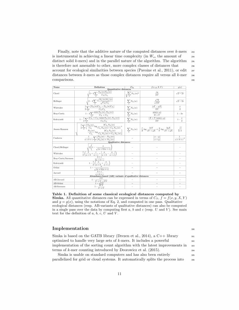
Finally, note that the additive nature of the computed distances over k-mers 293

is instrumental in achieving a linear time complexity (in Ws, the amount of 294

distinct solid k-mers) and in the parallel nature of the algorithm. The algorithm 295

is therefore not amenable to other, more complex classes of distances that 296

account for ecological similarities between species (Pavoine et al., 2011), or edit 297

distances between k-mers as those complex distances require all versus all k-mer 298

comparisons. 299

Name Definition CSi f(x, y,X, Y ) g(x)Quantitative distances

Chord

√2− 2

∑w

NSi(w)NSj

(w)

CSiCSj

√∑w

NSi(w)2

xy

XY

√2− 2x

Hellinger

√√√√2− 2∑w

√NSi(w)NSj (w)√

CSiCSj

∑w

NSi(w)

√xy

√XY

√2− 2x

Whittaker1

2

∑w

∣∣NSi(w)CSj

−NSj(w)CSi

∣∣CSiCSj

∑w

NSi(w)|xY − yX|

XY

x

2

Bray-Curtis 1− 2∑w

min(NSi(w), NSj (w))

CSi+ CSj

∑w

NSi(w)

min(x, y)

X + Y1− 2x

Kulczynski 1− 1

2

∑w

(CSi+ CSj

) min(NSi(w), NSj

(w))

CSiCSj

∑w

NSi(w)(X + Y ) min(x, y)

XY1− x

2

Jensen-Shannon

√√√√√√√√1

2

∑w

[NSi(w)

CSi

log2CSj

NSi(w)

CSjNSi

(w) + CSiNSj

(w)+

NSj(w)

CSj

log2CSi

NSj(w)

CSjNSi

(w) + CSiNSj

(w)

] ∑w

NSi(w)

x

Xlog

2xY

xY + yX+

y

Ylog

2yX

xY + yX

√x

2

Canberra1

a + b + c

∑w

∣∣∣∣NSi(w)−NSj (w)

NSi(w) + NSj

(w)

∣∣∣∣ −∣∣∣∣x− y

x + y

∣∣∣∣ 1

a + b + cx

Qualitative distances

Chord/Hellinger

√√√√2

(1− a√

(a + b)(a + c)

)− − −

Whittaker1

2

(b

a + b+

c

a + c+

∣∣∣∣ a

a + b− a

a + c

∣∣∣∣) − − −

Bray-Curtis/Sorensenb + c

2a + b + c− − −

Kulczynski 1− 1

2

(a

a + b+

a

a + c

)− − −

Ochiai 1− a√(a + b)(a + c)

− − −

Jaccardb + c

a + b + c− − −

Abundance-based (AB) variants of qualitative distances

AB-Jaccard 1− UV

U + V − UV− − −

AB-Ochiai 1−√UV − − −

AB-Sorensen 1− 2UV

U + V− − −

Table 1. Definition of some classical ecological distances computed bySimka. All quantitative distances can be expressed in terms of CS , f = f(x, y,X, Y )and g = g(x), using the notations of Eq. 2, and computed in one pass. Qualitativeecological distances (resp. AB-variants of qualitative distances) can also be computedin a single pass over the data by computing first a, b and c (resp. U and V ). See maintext for the definition of a, b, c, U and V .

Implementation 300

Simka is based on the GATB library (Drezen et al., 2014), a C++ library 301

optimized to handle very large sets of k-mers. It includes a powerful 302

implementation of the sorting count algorithm with the latest improvements in 303

terms of k-mer counting introduced by Deorowicz et al. (2015). 304

Simka is usable on standard computers and has also been entirely 305

parallelized for grid or cloud systems. It automatically splits the process into 306

11

jobs according to the available number of nodes and cores. These jobs are sent 307

to the job scheduling system, while the overall synchronization is performed at 308

the data level. 309

Simka is an open source software, distributed under GNU affero GPL 310

License, available for download at https://gatb.inria.fr/software/simka/. 311

Results 312

First, Simka performances are evaluated in terms of computation time, memory 313

footprint and disk usage and compared to those of other state of the art 314

methods. Then, the Simka distances are evaluated with respect to de novo and 315

reference-based distances and with respect to known biological results. 316

We conduct our numerical experiments on data from the Human 317

Microbiome Project (HMP) (Human Microbiome Project Consortium, 2012a) 318

which is currently one of the largest publicly available metagenomic datasets: 319

690 samples gathered from different human body sites 320

(http://www.hmpdacc.org/HMASM/). The whole dataset contains 2*16 billions 321

of Illumina paired reads distributed non uniformly across the 690 samples. One 322

advantage of this dataset is that it has been extensively studied, in particular 323

the microbial communities are relatively well represented in reference databases 324

(Human Microbiome Project Consortium, 2012a,b) (see 325

http://hmpdacc.org/pubs/publications.php for a complete list). Article S1 326

details precisely how the datasets used for each experiment were built. 327

Performance Evaluation 328

Performances on small datasets The scalability of Simka was first 329

evaluated on small subsets of the HMP project, where the number of compared 330

samples varied from 2 to 40. When computing a simple distance, such as 331

Bray-Curtis for instance, Simka running time shows a linear behavior with the 332

number of compared samples (Figure 3-A). As expected, counting the kmers for 333

each sample (MKC-count) consumes most of the time. This task has a 334

theoretical time complexity linear with the number of kmers, and thus the 335

number of samples, and this explains the observed linear behavior of the overall 336

program. In fact, most steps of Simka, namely MKC-count, MKC-merge and 337

simple distance computation, show a linear behavior between running time and 338

the number of compared samples. The only exception is the computation of 339

complex distances, where the time devoted to this task increases quadratically. 340

Both simple and complex distance computation algorithms have theoretical 341

worst case quadratic time complexity relatively to N (the number of samples). 342

The difference of execution time comes then from the amount of operations 343

required, in practice, to calculate the crossed terms of the distances. For a given 344

abundance vector, the simple distances only need to be updated for each pair 345

(Si, Sj) such that NSi> 0 and NSj

> 0 whereas complex distances need to be 346

updated for each pair such that NSi> 0 or NSj

> 0, entailing a lot more 347

12

update operations. It is noteworthy that among all distances listed in Table 1, 348

all distances are simple, except the Whittaker, Jensen-Shannon and Canberra 349

distances. 350

When compared to other state of the art tools, namely Commet, Metafast 351

and Mash, we parameterized Simka to compute only the Bray-Curtis distance, 352

since all other tools compute only one such simple distance. The Fig. 3-B-C-D 353

shows respectively the CPU time, the memory footprint and the disk usage of 354

each tool with respect to an increasing number of samples N . Mash has 355

definitely the best scalability but limitations of its computed distance are shown 356

in the next section. Commet is the only one to show a quadratic time behaviour 357

with N . For N = 40, Simka is 6 times faster than Metafast and 22 times faster 358

than Commet. All tools, except Metafast, have a constant maximal memory 359

footprint with respect to N . For metafast, we could not use its max memory 360

usage option since it often created ”out of memory” errors. The disk usage of 361

the four tools increases linearly with N . The linear coefficient is greater for 362

Simka and MetaFast, but it remains reasonable in the case of Simka, as it is 363

close to half of the input data size, which was 11 GB for N = 40. 364

In summary, Simka and Mash seems to be the only tools able to deal with 365

very large metagenomics datasets, such as the full HMP project. 366

Performances on the full HMP samples Remarkably, on the full dataset 367

of the HMP project (690 samples), the overall computation time of Simka is 368

about 14 hours with very low memory requirements (see Table 2). By 369

comparison, Metafast ran out of memory (it also ran out of memory while 370

considering only a sub-sample composed of the 138 HMP gut samples) and 371

Commet took several days to compute one 1-vs-all distance matrix and 372

therefore would require years of computation to achieve the N ×N distance 373

matrix. Conversely, Mash ran in less than 5 hours (255 min) and is faster than 374

Simka. This was expected since Mash outputs an approximation of a simple 375

qualitative distance, based on a sub-sample of 10,000 k-mers. By comparison, 376

Simka computes numerous distances, including quantitative ones, over 15 billion 377

distinct k-mers (see Table 2). Note that Simka is also designed for coarse-grain 378

parallelism, and such computation took less than 10 hours on a 200-CPU 379

platform. 380

These results were obtained with default parameters, namely filtering out 381

k-mers seen only once. On this dataset, this filter removes only 5 % of the data: 382

solid k-mers (k-mers seen at least twice) account for 95% of all base pairs of the 383

whole dataset (see Table 2). But interestingly, when speaking in terms of 384

distinct k-mers, solid distinct k-mers represent less than half of all distinct 385

k-mers before merging across all samples and only 15% after merging. 386

Consequently, Simka performances are greatly improved, both in terms of 387

computation time and disk usage when considering only solid k-mers. Notably, 388

this does not degrade distance quality, at least for the HMP dataset, as shown 389

in the next section. Additional tests on the impact of k on the performances 390

show that the disk usage increases sub-linearly with k whereas the computation 391

13

0

25

50

75

100

2 5 10 20 40Samples

CP

U ti

me

(min

)Simka

Complex distances

Simple distances

MKC−Merge

MKC−Count

A

● ● ● ●●

0

100

200

300

400

500

2 5 10 20 40Samples

CP

U ti

me

(min

)

● Simka

Commet

Metafast

Mash

B

● ● ● ● ●

0

5

10

15

20

25

2 5 10 20 40Samples

Mem

ory

(GB

)

● Simka

Commet

Metafast

Mash

C

●●

●

●

●

0

5

10

15

2 5 10 20 40Samples

Dis

k (G

B)

● Simka

Commet

Metafast

Mash

D

Figure 3. Simka performances with respect to the number N of inputsamples. Each dataset is composed of two million reads. All tools were run on amachine equipped with a 2.50 GHz Intel E5-2640 CPU with 20 cores, 264 GB ofmemory. (A) and (B) CPU time with respect to N . For (A), colors correspond todifferent main Simka steps. (C) Memory footprint with respect to N . (D) Disk usagewith respect to N . Parameters and command lines used for each tool are detailed inTable S1.

time and the memory usage stay constant (see Fig. S1). 392

Evaluation of the distances 393

We evaluate the quality of the distances computed by Simka answering two 394

questions. First, are they similar to distances between read sets computed using 395

other approaches? Second, do they recover the known biological structure of 396

HMP samples? For the first evaluation, two types of other approaches are 397

14

HMP - 690 samples - 3727 GB - 2×16 billion paired readsWithout filter With filter

Number of k-mers 2471× 109 2331× 109

Number of distinct k-mers before merging 251× 109 111× 109

Number of distinct k-mers after merging 95× 109 15× 109

Memory (GB) 62 62Disk (GB) 1661 795Total time (min) 1338 862

MKC-Count (min) 758 573MKC-Merge (min) 148 77Simple distances (min) 432 212

Complex distances (min) 8957 4160

Table 2. Simka performances and k-mer statistics of the whole HMPproject (690 samples) Simka was run on a machine equipped with a 2.50 GHz IntelE5-2640 CPU with 20 cores, 264 GB of memory, with k = 31. Numbers of distinctk-mers are computed before and after the MKC-Merge algorithm: the before mergingnumber is obtained by summing over all samples the distinct k-mers computed foreach sample independently, whereas in the after merging number, k-mers shared byseveral samples are counted only once. Line “Total time” does not include complexdistances whose computation is optional.

considered, either de novo ones (similar to Simka but based on read 398

comparisons), or taxonomic distances, e.g. approaches based on a reference 399

database. 400

Correlation with read-based approaches In this section, we focus on 401

comparing Simka k-mer-based distance to two read-based approaches: 402

Commet (Maillet et al., 2014) and an alignment-based method using 403

BLAT (Kent, 2002). Both these read-based approaches define and use a read 404

similarity notion. They derive the percentage of reads from one sample similar 405

to at least one read from the other sample as a quantitative similarity measure 406

between samples. Commet considers that two reads are similar if they share at 407

least t non-overlapping k-mers (here t = 2, k = 33). For BLAT alignments, 408

similarity was defined based on several identity thresholds: two reads were 409

considered similar if their alignment spanned at least 70 nucleotides and had a 410

percentage of identity higher than 92%, 95% or 98%. For ease of comparison, 411

Simka distance was transformed to a similarity measure, such as the percentage 412

of shared kmers (see Article S1 for details of transformation). 413

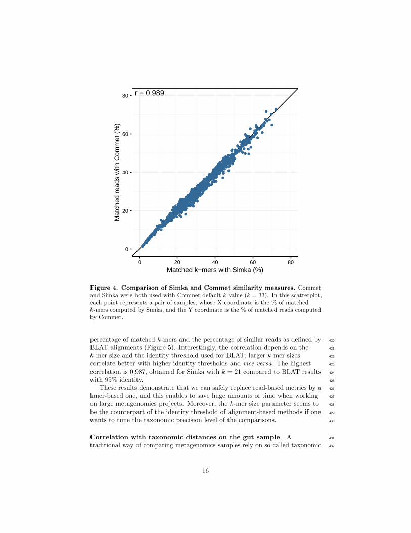
Looking at the correlation with Commet is interesting because this tool uses 414

a heuristic based on shared k-mers but its final distance is expressed in terms of 415

read counts. As shown in Figure 4, on a dataset of 50 samples from the HMP 416

project, Simka and Commet similarity measures are extremely well correlated 417

(Spearman correlation coefficient r = 0.989). 418

Similarly, clear correlations (r > 0.89) are also observed between the 419

15

●

●

●●

●

●

●

●

●

●

●

●

●

●

●

●

●

●

●

●

●

●

●

●

●

●

●

●

●

●● ●

●

●●

●

●

●

●

●

●

●

●

●

●

●

●

●

●

●

●

●

●

●

●

●

●●

●

●

●

●

●●●

●●

●●

●

●

●

●

●

●

●●

●

●

●

●

●

●

●

●

●

●●

●

●

●

●

●

●

●

●

●

●

●

●

●

●

●

●

●

●

●●

●

●

●

●●

●

●

●

●

●

●

●

●

●

●●

●●●

●

●

●

●

●

●

●

●

●

●●

●

●

●

●

●

●

●

●

●

●

●

●

●

●

●

●

●

●

●

●

●

●

●●

●

●●

●

●

●

●

●

●

●

●

●

●

●

●

●

●

●

●

●

●

●

●●

●

●

●

●

●

●

●

●

●

●

●●

●

●

●

●

●

●

●

●

●

●

●

●

●●

●

●

●

●

●

●

●

●

●

●

●

●●

●

●●

●

●

●

●

●

●

●

●

●

●

●

●

●

●

●

●

●

●

●

●

●

●

●

●●

●

●

●

●

●

●

●

●

●

●

●

●

●

●

●

●

●

●

●

●

●

●

●

●

●

●

●

●

●

●

●

●

●

●

●

●

●

●

●

●

●

●●

●

●

●

●

●

●

●

●

●

●

●

●

●

●

●

●

●

●

●

●

●

●

●

●●

●

●

●

●

●

●

●

●

●

●

●

●

●

●

●

●

●

●

●

●

●

●

●

●

●

●

●

●

●

●

●

●

●

●

●

●

●

●

●

●

●●

●●

●

●

●

●

●

●

●●●

●●

●

●●

●

●

●

●

●

●

●

●

●

●

●

●

●

●●

●

●

●●

●

●

●

●

●

●

●

●

●

●

●

●

●

●

●

●●

●

●●

●

●●

●

●●

●

●●

●

●

●

●

●

●

●

●

●

●

●

●

●

●

●●

●

●

●●

●

●

●

●

●

●

●

●

●

●

●

●

●

●●

●

●

●

●

●

●

●

●

●

●

●

●

●●

●

●

●

●

●

●

●

●

●

●

●

●

●

●

●

●

●

●

●

●

●

●

●●

●

●

●

●●

●

●

●

●

●

●

●

●

●

●●

●●●

●

●

●

●

●

●

●

●

●

●

●

●

●

●

●●

●

●

●

●

●

●

●

●

●

●

●

●

●●

●

●

●

●

●●

●

●

●

●●

●

●

●

●●

●

●●

●

●

●

●

●

●

●

●

●

●

●

●

●

●

●

●

●

●

●

●

●

●

●

●●

●

●

●●●

●

●

●

●

●

●

●●

●

●

●●

●

●

●

●

●

●

●

●●●

●

●

●●

●

●

●

●

●

●

●

●

●

●

●

●

●

●

●

●

●

●

●

●

●

●●

●

●

●

●

●

●

●

●

●

●●

●

●

●

●

●

●

●

●

●

●

●●

●●●

●

●

●

●

●

●

●

●

●

●

●

●

●

●

●

●

●

●

●

●

●

●●

●

●

●

●

●

●

●●

●

●

● ●●

●

●

●

●

●

●

●

●●

●

●●

●

●

●

●

●

●

●

●

●

●

●

●

●

●

●

●

●

●

● ●

●

●

●●

●

●

●

●

●

●

●

●

●

●

● ●

●

●

●●

●

●

●

●

●

●

●

●

●

●

●

●

●

●

●

●

●

●

●

●

●●

●

●

●

●

●

●

●

●

●

●

●

●

●

●

●

●

●

●

●

●

●

●

●

●

●

●

●

●

●

●

●

●

●

●●

●

●

●

●

●

●

●

●

●

●

●

●

●

●

●

●

●

●

●

●

●

●

●

●●

●

●

●

●

●

●

●

●

●

●●

●

●

●

●●

●●●

●

●

●

●

●

●●

●

●

●

●

●

●

●

●

●

●

●

●

●

●●

●

●●

●

●

●

●

●

●

●

●

●

●

●

●

●

●

●

●

●

●

●

●●

●

●

●

●

●

●

●

●

● ●

●

●

●●

●●

●

●

●

●

●●

●

●

●

●

●

●

●

●

●

●●

●

●

●

●

●

●

●

●●

●

●

●

●

●

●

●

●

●

●

●

●●

●

●

●

●

●

●

●

●

●

●

●

●

●

●

●

●

●

●

●

●

●

●

●

●

●

●●

●

●

●

●●●

●

●

●

●

●

●

●

●

●

●

●

●

●

●

●

●

●●

●

●

●

●●

●

●

●

●

●

●

●

●

●

●

●

●

●

●

●

●●

●

●

●

●

●

●

●

●●

●

●●

●

●●

●

●

●

●

●

●

●

●

●

●

●

●●

●

●

●●

●

●

●

●

●

●

●

●

●

●

●

●

●

●

●

●●

●

●

●

●

●

●

●

●●

●

●

●

●

●

●

●

● ●

●

●

●

●

●

●

●

●

●

●

●

●

●

●

●

●

●

●

●

●

●

●

●

●

●

●

●

●

●

●

●

●

●

●

●

● ●

●

●

●

●

●●

●

●

●

●

●

●

●

●

●

●

●

●

●

●

●

●●

●

●

●

●

●

●

●

●

●

●

●

●

●

●

●

●

●

●

●

●

●●

●

●

●●

●

●

●●

●

●

●

●

●

●

●

●

●

●

●

●

●

●

●

●

●

●

●

●

●

●

●

●

●

●

●

●

●

●●

●

●

●

●

●

●

●

●

●●

●

●

● ●

●

●

●

●

●

●

●

●

●

●

●

●

●●

●●

●

● ●

●

●

●●

●

●

●

●

●

●

●

●

●

●

●

●

●

●●

●

●

●

●

●

●

●

●

●

●

●

●

●

●

●

●

●

●

●

●

●●

●

●

●

●

●

●

●

●

●

●

●●

●

●

●

●

●

●

●

●

●

●

●

●

●

●

●

●

●●

●

●

●

●●

●

●

●

●

●

●

●

●

●

●

●

● ●

●

●

●

●

●

●

●

●●

●

●

●

●

●

●

●

●

●

●

●

●

●

●

●

●

●

●●

●

●

●●

●

●

●

●

●

●

●

●

●

●

●

●

●

●

●

●

●

●

●

●

●

●

●

●

●

●

●

●

●

●

●

●●

●

●

●

●

●

●

●

●

●

●

●

●

●

●●

●

●

●

●

●

●

●

●

●

●

●

●

●

●

●

●

●●

●

●

●●

●

●●

●●●

●

●●

●

●

●

●

●

●

●

●

●

●

●

●

●

●

●

●

●●

●

●

●

●

●

●

●

●

●

●

●

●

●

●

●

●

●

●

●

● ●

●

●

●

●

●

●

●

●

●

●

●

●

●

●

●

●

●

●

●

●

●

●

●

●

●

●

●

●

●

●

●

●

●

●

●

●

●●●

●

●●

●

●

●

●

●

●

●

●

●●

●

●

●

●

●

●

●

●

●

●

●

●

●

●

●

●

●

●

●

●

●

●

●

●

●

●

●

●●

●

●

●

●

●

●

●

●

●

●●

●

●

●

●

●

●

●

●

●

●

●

●

●

●

●

●

●

●●

●

●

●

●

●

●

●

●

●

●

●

●

●

●

●

●

●

●

●

●

●

●

●

●

●●

●

●

●

●

●

●

●

●

●●

●

●

●

●

●

●

●

●

●●

●

●

●

●

●

●

●

●

●

●

●●

●

●

●

●

●

●

●

●

●●

●

●

●●

●

●●

●

●

●

●

●

●

●

●

●

●

●

●

●●

●

●

●●

●●

●

●

●

●

●

●

●

●

●

●

●

●

●

●

●

●

●

●

●

●

●

●

●

●

●●

●

●

●

●

●

●

●

●

●

●

●

●

●

●●

●

●

●

●

●●

●

●

●

●

●

●

●

●

●

●

●

●

●

●

●

●●

●

●

●

●

●

●

●

●

●

●

●

●

●

●

●

●

●

●

●

●

●●

●

●

●●

●

●

●

●●

●

●

●

●

●

●

●

●

●

●

●

●

●

●

●

●

●●

●

●

●

●

●

●

●●

●

●

●

●

●

●

●

●●

●

●

●

●

●

●

●

●●

●

●

●

●

●

●

●●

●

●

●

●

●

●

●

●

●

●

●

●

●

●

●

●

●

●

●

●

●

●●

●

●

●

●

●

●

●

●

●

●

●

●

●

●

●

●●

●

●

●

●

●●

●

●

●

●

●

●

●

●

●

●

●

●

●

●

●

●

●

●

●

●

●

●

●

●

●

●

●

●

●

●

●

●

●

●

●

●

●

●

●

●

●

●●

●●●

●

●

●

●●

●

●

●

●

●

●

●

●

●

●

●

●

●

●

●

●

●

●

●

●

●

●

●●

●

●

●

●

●

●●

●●

●

●

●

●

●

●

●

●

●

●

●

●

●

●

●●

●

●

●

●

●

●

●

●

●

●●

●

●

●

●

●

●

●●

●

●

●

●●

●

●

●

●

●

●●

●

●

●

●

●●

●

●

●

●

●

●

●

●

●

●●

●

●

●

●

●

●

●

●

●

●

●

●

●

●

●

●

●

●

●

●

●

●

●

●●

●

●

●

●

●

●●

●

● ●

●

●

●

●

●

●●

●●

●

●

●

●

●●

●

●

●

●

●

●

●

●

●

●

●

●

●

●

●

●

●

●

●

●

●

●

●●

●

●

●

●

●

●●

●●

●

●

●

●

●

●

●

●

●●

●

●

●

●

●

●

●

●

●

●

●

●

●

●

●

●

●

●

●

●

●

●

●

●●

●

●

●

●

●

●

●

●

●

●

●

●

●●

●

●

●●

●

●

●

●

●

●

●

●

●

●●

●

●

●

●

●

●

●

●

●

●

●

●

●

●

●

●

●

●

●

●

●

●

●

●

●

●

●

●

●

●

●

●

●

●

●

●

●

●

●

●

●●

●

●●

●

●

●

●

●

●

●

●

●

●

●

●

●

●

●

●

●

●

●

●

●

●

●

●

●

●

●

●

●

●

●●

●

●

●

●

●

●

●

●●

●●

●

●

●

●

●

●

●

●●

●●●●

●

●●

●

●

●●

●

●

●

●

●

●

●

●

●

●

●

●

●

●●

●

●

●

●

●

●●

●

●

●

●

●

●

●

●

●●

●

●

●

●

●

●

●

●

●

●

●

●

●

●

●

●

●

●

●

●

●

●

●

●

●

●

●

●

●

●

●

●

●

●

●

●

●

●

●

●

●

●

●

●

●

●

●

●●

●●

●

●

●

●

●●

●

●

●

●

●

●

●

●

●

●

●

●

●

●

●

●

●

●

●

●

●

●

●

●

●

●

●

●

●●

●●

●

●

●●

●●

●

●

●●●●

●

●●

●●●●

●

●●●

●●●

●●

●

●

●

r = 0.989

0

20

40

60

80

0 20 40 60 80

Matched k−mers with Simka (%)

Mat

ched

rea

ds w

ith C

omm

et (

%)

Figure 4. Comparison of Simka and Commet similarity measures. Commetand Simka were both used with Commet default k value (k = 33). In this scatterplot,each point represents a pair of samples, whose X coordinate is the % of matchedk-mers computed by Simka, and the Y coordinate is the % of matched reads computedby Commet.

percentage of matched k-mers and the percentage of similar reads as defined by 420

BLAT alignments (Figure 5). Interestingly, the correlation depends on the 421

k-mer size and the identity threshold used for BLAT: larger k-mer sizes 422

correlate better with higher identity thresholds and vice versa. The highest 423

correlation is 0.987, obtained for Simka with k = 21 compared to BLAT results 424

with 95% identity. 425

These results demonstrate that we can safely replace read-based metrics by a 426

kmer-based one, and this enables to save huge amounts of time when working 427

on large metagenomics projects. Moreover, the k-mer size parameter seems to 428

be the counterpart of the identity threshold of alignment-based methods if one 429

wants to tune the taxonomic precision level of the comparisons. 430

Correlation with taxonomic distances on the gut sample A 431

traditional way of comparing metagenomics samples rely on so called taxonomic 432

16

●

●

●

●

●

●

●

●

●

0.875

0.900

0.925

0.950

0.975

1.000

15 21 31

k−mer size

Spe

arm

an c

orre

latio

n

BLATalignmentidentity (%)

●

●

●

92

95

98

Figure 5. Comparison of Simka and BLAT distances for several values ofk and several BLAT identity thresholds. Spearman correlation values arerepresented with respect to k. The scatterplots obtained for each point of this figureare shown in Fig. S2).

distances that are based on sequence assignation to taxons by mapping to 433

reference databases. To compare Simka to such traditional reference-based 434

method, we used the HMP gut samples, which is a well studied dataset 435

comprising 138 samples. The HMP consortium provides a quantitative 436

taxonomic profile for each sample on its website. These profiles were obtained 437

by mapping the reads on a reference genome catalog at 80% of identity. From 438

these profiles, we computed the Bray-Curtis distance, latter used as a reference. 439

The complete protocol to obtain taxonomic distances is given in Article S1. 440

Only Mash and Simka results have been considered for this experiment. As 441

previously mentioned, Commet and MetaFast could not scale this dataset. 442

Simka k-mer-based distance appears very well correlated to the traditional 443

taxonomic distance (r = 0.89, see Fig. 6). On this figure, one may also notice 444

that Simka measures are robust with the whole range of distances. On the other 445

hand, Mash distances correlate badly with taxonomic ones (r = 0.51, see Fig. S3 446

and the comparison protocol in Article S1). This is probably due to the fact 447

17

that gut samples differ more in terms of relative abundances of microbes than in 448

terms of composition (see next section). As Mash can only output a qualitative 449

distance, it is ill equipped to deal with such a case. Additionally, as shown in 450

Fig. S3, this conclusion stands for the HMP samples from other body sites for 451

which one disposes of high quality taxonomic distances. 452

Interestingly, these Simka results are robust with the k-mer filtering option 453

and the k-mer size, as long as k is larger than 15 and with an optimal 454

correlation obtained with k = 21 (see Fig. S4). Notably, with very low values of 455

k (k < 15), the correlation drops (r = 0.5 for k = 12). This completes previous 456

results suggesting that the larger the k the better the correlation, that were 457

limited to k values smaller than 11 (Dubinkina et al., 2016). 458

r = 0.885

0.25

0.50

0.75

1.00

0.25 0.50 0.75 1.00

Taxonomic distance

Sim

ka d

ista

nce

1

10

100count

Figure 6. Correlation between taxonomic distance and k-mer baseddistance computed by Simka on HMP gut samples. On this density plot, eachpoint represents one or several pairs of the gut samples. The X coordinate indicatesthe Bray-Curtis taxonomic distance, and the Y coordinate the Bray-Curtis distancecomputed by Simka with k = 21. The color of a point is function of the amount ofsample pairs with the given pair of distances (log-scaled).

18

Visualizing the structure of the HMP samples We propose to visualize 459

the structure of the HMP samples and see if Simka is able to reproduce known 460

biological results. To easily visualize those structures, we used the Principal 461

Coordinate Analysis (PCoA) (Borg and Groenen, 2013) to get a 2-D 462

representation of the distance matrix and of the samples: distances in the 2-D 463

plane optimally preserve values of the distance matrix. 464

Fig. 7 shows the PCoA of the quantitative Ochiai distance computed by 465

Simka on the full HMP samples. We can see that the samples are clearly 466

segregated by body sites. This is in line with results from studies of the HMP 467

consortium (Human Microbiome Project Consortium, 2012a; Costello et al., 468

2009; Koren et al., 2013). Moreover, one may notice that different distances can 469

lead to different distributions of the samples, with some clusters being more or 470

less discriminated (see Fig. S5). This confirms the fact that it is important to 471

conduct analyses using several distances as suggested in (Koren et al., 2013; 472

Legendre and De Caceres, 2013) as different distances may capture different 473

features of the samples. 474

We conduct the same experiment on the 138 gut samples from the HMP 475

project. Arumugam et al. (2011) showed that the gut samples are organized in 476

three groups, known as enterotypes, and characterized by the abundance of a 477

few genera: Bacteroides, Prevotella and genera from the Ruminococcaceae 478

family. The original enterotypes were built from Jensen-Shannon distances on 479

taxonomic profiles. The Fig. 8 shows the PCoA of the Jensen-Shannon 480

distances obtained with Simka. Mapping the relative abundance of those genera 481

in each sample, as provided by the HMP consortium, on the 2-D representation 482

reveals a clear gradient in the PCoA space. Simka distances therefore recover 483

biological features it had no direct access to: here, the fact that gut samples are 484

structured along gradients of Bacteroides, Prevotella and Ruminococcaceae. The 485

fact that Simka is able to capture such subtle signal raises hope of drawing new 486

interesting biological insights from the data, in particular for those 487

metagenomics project lacking good references (soil, seawater for instance). 488

Discussions 489

In this article, we introduced Simka, a new method for computing a collection of 490

ecological distances, based on k-mer composition, between many large 491

metagenomic datasets. This was made possible thanks to the Multiple k-mer 492

Count algorithm (MKC), a new strategy that counts k-mers with 493

state-of-the-art time, memory and disk performances. The novelty of this 494

strategy is that it counts simultaneously k-mers from any number of datasets, 495

and that it represents results as a stream of data, providing counts in each 496

dataset, k-mer per k-mer. 497

The distance computation has a time complexity in O(W ×N2), with W is 498

the number of considered distinct k-mers and N is the number of input samples. 499

N is usually limited to a few dozens or hundreds and can not be reduced. 500

However, W may range in the hundreds of billions. The solid filter already 501

19

●

●

●●

●

●

●

●

●

●

●

●

●

●

●

●

●

●

●

●●

●

●

●

●

●

●

●

●

●

●

●

●

●

●

●

●

●

●

●

●●

●

●

●

●

●

● ●

●

●

●

●

●

●

●

●

● ●

●

●

●

●

●

●

●●

●

●

●

●

●

●

●

●●

●●

●

●●

●

●

●

●

●

●●

●

●

●

●

●

●

●

●

●

●

●

●

●●●●

●●

●

●

●

●

●

●

●

● ●

●

●

●

●

●

●●

●

●

●

●

●

●

●●

●

●●●

●●

●

●

●

●

●

●

●

●

●

●

●

●

●

●

●

●

●●

●

●

●

●●●

●●

●

●

●

●●

●●

●

●

●●

●

●

●

●

●● ●

●●

●●

●

●

●

●●

●

●

●

●

●

●

●

●

●

●●

● ●

●

●

●

●

●

●

●

●

●

●●

●

●

●

●

●

●

●

●●

●

●●

●

●

●

●

●

●●

●

●

●

●

●

●

●

●

●

●●

●

●

●

●●

●

●

●

●

●

●●

●

●

●

●

●

●

●

●●

●

●

●●

●

●

●●

●●

●

●

●●●

●

●●

●

●

●

●

●

●

●

●

●

●

●

●

●

●

●●

●

●

●●●

●

●

●

●

●

●

●

●

●

●

●

●●●●

●

●●

●

●

●

●●

●

●

●●

●

●

●●

●

●

●

●

●

●●

●

●

●

●●

●

●

●●

●●

● ●●

●

●

●

●

●

●●

●

●

●

●

●●

●

●●

●

●

●

●

●●

●●

●

●●●

●

●

●

●●

●

●

●

●●

●

●

●

●●

●

●

●●

●

●

●

●

●

●

●

●

●

●●

●

●

●

●

●

●

●

●

●

●

●

●

●

●

●●

●

●

●●

●

●

●

●

●

●

●

●

●

●

●

●●

●●

●

●●

●

●

●

●

●

●

●

●

●

●

●

●

●

●

●

●●

●

●

●

●

●

●

●

●

●

●●

●●

●

●

●

●

●

●

●

●

●

●

●

●

●

●

●

● ●

●

●

●

●

●

●

●

●

●

●

●

●

●

●

●

●

●

●

●

●

●

●

●

●

●

●

●

● ●

●●

●●

●

●●

●

●

●

●

●

●

●

●

●

●●

●

●

●

●

●

●

●

●

●

●

●

●

●

●

●

●

●

●

●

●

●

●●

●●

●

●

●

●

●

●

●

●

●

●

●

●

●

●

●

●

●

●

● ●●

●

●

●

●●

●

●

●

●

●

●

●●

●

●

●

●

●

●

●

●●

●

●

●

●

●

●

●

●

●

●

●

●

●

●

●

●

●●

●

●

●

● ●

●

●

●

●

●

●●

●

●

●

●

●

●

●●

●●●

●

●●

●

●

●

●

●

●

●

●●

●

●

●

●●

●

●

●

●

●

●

●

●

●

●●

●

●

●

●

●

●●

Gastrointestinal

Oral

Urogenital

Nasal

Skin

PC1 (18.73%)

PC

2 (1

2.37

%)

Figure 7. Distribution of the diversity of the HMP samples by body sites.PCoA of the samples is based on the quantitative Ochiai distance computed by Simkawith k = 21. Each dot corresponds to a sample and is coloured according to thehuman body site it was extracted from. The green color shades correspond to 3different subparts of the Oral samples: Tongue dorsum, Supragingival plaque, Buccalmucosa (from top to down).

provides large speed improvement without affecting the results, at least on the 502

tests performed on the HMP datasets. However, the HMP dataset is not 503

representative of all metagenomics projects and, in some cases, this filter may 504

not be desired. For instance, in the case of samples with low coverage or when 505

performing qualitative studies where the rare species have more impact. As a 506

matter of fact, it is notable that Simka is able to scale large datasets even with 507

the solid filter disabled as shown in the performance section. Interestingly, when 508

applied on a low coverage dataset, namely the Global Ocean Sampling (Yooseph 509

et al., 2007), Simka was able to capture the essential underlying biological 510

structure with or without the k-mer solid filter (see Fig. S6). However, an 511

important incoming challenge is to precisely measure the impact of applied 512

thresholds together with the choice of k, depending on the input dataset 513

features such as community complexity and sequencing effort. 514

20

●●

●

●

●

●

●

●

●

●

●●

●

●

●

●

●

●●

●

●

● ●

●

●●

●●

●

●

●

●●

●

●

●

● ●

●

●●

●

●

●

●

●

●

●

●

●

●

●

●

●

●●

● ●

●

●

●

●

●●

●

●●

●

●

●

●

●

●

●●

●●●

●

●

●

●

●

●

●

●

●

●

●●

●●

●

●

●●

●

●●

●

●

●

●

●

●

●

●

●

●

●

●

●

●

●

●

●

●

●

●

●

●

● ●●

●

●

●

●

●

●

●●

●

●●

●●

●

PC1 (6.15%)

PC

3 (3

.53%

)

25

50

75

Abundance (%)

A Bacteroides

●●

●

●

●

●

●

●

●

●

●●

●

●

●

●

●

●●

●

●

● ●

●

●●

●●

●

●

●

●●

●

●

●

● ●

●

●●

●

●

●

●

●

●

●

●

●

●

●

●

●

●●

● ●

●

●

●

●

●●

●

●●

●

●

●

●

●

●

●●

●●●

●

●

●

●

●

●

●

●

●

●

●●

●●

●

●

●●

●

●●

●

●

●

●

●

●

●

●

●

●

●

●

●

●

●

●

●

●

●

●

●

●

● ●●

●

●

●

●

●

●

●●

●

●●

●●

●

PC1 (6.15%)

PC

3 (3

.53%

)

0

20

40

60

Abundance (%)

B Prevotella

●●

●

●

●

●

●

●

●

●

●●

●

●

●

●

●

●●

●

●

● ●

●

●●

●●

●

●

●

●●

●

●

●

● ●

●

●●

●

●

●

●

●

●

●

●

●

●

●

●

●

●●

● ●

●

●

●

●

●●

●

●●

●

●

●

●

●

●

●●

●●●

●

●

●

●

●

●

●

●

●

●

●●

●●

●

●

●●

●

●●

●

●

●

●

●

●

●

●

●

●

●

●

●

●

●

●

●

●

●

●

●

●

● ●●

●

●

●

●

●

●

●●

●

●●

●●

●

PC1 (6.15%)

PC

3 (3

.53%

)

10

20

30

40

50

Abundance (%)

C Ruminococcaceae

Figure 8. Relative abundances of main genera in HMP gut samples.Distribution of the gut samples from the HMP project is shown in a PCoA of theJensen-Shannon distance matrix. This distance matrix was computed by Simka withk = 21. Relative abundances (0-100%) of (A) Bacteroides, (B) Prevotella and (C)Ruminococcaceae, as computed with Metaphlan (Segata et al., 2012), are mapped ontothe sample points as color shades.

21

Since metagenomic projects are constantly growing, it is important to offer 515

the possibility to add new sample(s) to a set for which distances are already 516

computed, without starting back the whole computation from scratch. It is 517

straightforward to adapt the MKC algorithm to such operation, but the 518

merging step and distance computation step have to be done again. However, 519

adding a new sample does not modify previously computed distances and only 520

requires to compute a single line of the distance matrix, it can thus be achieved 521

in linear time. 522

The motivation for computing a collection of distances rather than just one 523

is two folds: different distances capture different features of the data (Koren 524

et al., 2013; Legendre and De Caceres, 2013; Pavoine et al., 2011) and all the 525

distances computed by Simka have in common that they are additive over 526

k-mers and can thus be computed simultaneously using the same algorithm. To 527

support the first point, we have seen that Mash performed badly when 528

considering HMP samples per body sites since this tool can only take into 529

account presence/absence information and not relative abundances in contrast 530

to Simka. As a matter of fact, differences in relative abundances are subtler 531

signals that are often at the heart of interesting biological insights in 532

comparative genomics studies. For instance, Boutin et al. (2015) showed that 533

the structure between different samples from lung disease patients was visible 534

with the Bray Curtis (quantitative) distance and absent with the qualitative 535

Jaccard distance, highlighting the role of the abundances of certain pathogenic 536

microbes in the disease. In other studies, the response of bacterial communities 537

to stress or environmental changes was shown to be driven by the increase in 538

abundance of some rare taxa (Shade et al., 2014; Genitsaris et al., 2015; Coveley 539

et al., 2015; Gomez-Alvarez et al., 2016). 540

A notable key point of our proposal is to estimate beta-diversity using 541

k-mers diversity only. We are conscious this may lead to biased estimates of the 542

beta-diversities defined from species composition data. The bias can run both 543

ways: on the one hand, shared genomic regions or horizontal transfers between 544

species will bias the k-mer-based distance downwards. On the other hand, 545

genome size heterogeneity and k-mer composition variation along a microbe 546

genome will bias the k-mer-based distance upwards. However, species 547

composition based approaches are not feasible for large read sets from complex 548

ecosystems (soil, seawater) due to the lack of good references and/or mapping 549

scaling limitations. Moreover, our proposal has the advantage of being a de 550

novo approach, unbiased by reference banks inconsistency and incompleteness. 551

Finally, numerical experiments on the HMP datasets show that k-mer based and 552

taxonomic distances are well correlated (r > 0.8 for k ≥ 21) and consequently 553

that Simka recovers the same biological structure as taxonomic studies do. 554

There is nevertheless room for improving Simka distances. For instance, 555

recently, Brinda et al. (2015) showed that spaced seeds can improve the 556

k-mer-based metagenomic classification obtained with the popular tool 557

Kraken (Wood and Salzberg, 2014). Spaced seeds can be seen as non-contiguous 558

k-mers allowing therefore a certain number of mismatches when comparing 559

them. Being less stringent when comparing k-mers could lead to more accurate 560

22

distances, especially for viral metagenomic fractions which contain a lot of 561

mutated sequences. 562

Acknowledgments 563

Authors warmly thank, Olivier Jaillon and Thomas Vannier from Genoscope 564

(CEA - IG - LAGE) and Stephane Robin from INRA AgroParisTech for 565

providing their technical, biological and statistical expertise, as well as feedback 566

during the conception of this manuscript. We thank the GenOuest 567

BioInformatics Platform that provided the computing resources necessary for 568

benchmarking. 569

References

S. F. Altschul, W. Gish, W. Miller, E. W. Myers, and D. J. Lipman. Basic localalignment search tool. Journal of molecular biology, 215(3):403–410, 1990.

M. Arumugam, J. Raes, E. Pelletier, D. Le Paslier, T. Yamada, D. R. Mende,G. R. Fernandes, J. Tap, T. Bruls, J.-M. Batto, M. Bertalan, N. Borruel,F. Casellas, L. Fernandez, L. Gautier, T. Hansen, M. Hattori, T. Hayashi,M. Kleerebezem, K. Kurokawa, M. Leclerc, F. Levenez, C. Manichanh, H. B.Nielsen, T. Nielsen, N. Pons, J. Poulain, J. Qin, T. Sicheritz-Ponten, S. Tims,D. Torrents, E. Ugarte, E. G. Zoetendal, J. Wang, F. Guarner, O. Pedersen,W. M. de Vos, S. Brunak, J. Dore, J. Weissenbach, S. D. Ehrlich, and P. Bork.Enterotypes of the human gut microbiome. Nature, 473(7346):174–180, 052011.

I. Borg and P. Groenen. Modern Multidimensional Scaling: Theory andApplications. Springer Series in Statistics. Springer New York, 2013. ISBN9781475727111.

S. Boutin, S. Y. Graeber, M. Weitnauer, J. Panitz, M. Stahl, D. Clausznitzer,L. Kaderali, G. Einarsson, M. M. Tunney, J. S. Elborn, M. A. Mall, and A. H.Dalpke. Comparison of microbiomes from different niches of upper and lowerairways in children and adolescents with cystic fibrosis. PLoS ONE, 10(1):1–19, 01 2015. doi: 10.1371/journal.pone.0116029.

K. Brinda, M. Sykulski, and G. Kucherov. Spaced seeds improve k-mer-basedmetagenomic classification. Bioinformatics, 31(22):3584–3592, 2015.

A. Z. Broder. On the resemblance and containment of documents. InCompression and Complexity of Sequences 1997. Proceedings, pages 21–29.IEEE, 1997.

L. Cai, L. Ye, A. H. Y. Tong, S. Lok, and T. Zhang. Biased diversity metricsrevealed by bacterial 16s pyrotags derived from different primer sets. PLoSOne, 8(1):e53649, 2013.

23

A. Chao, R. L. Chazdon, R. K. Colwell, and T.-J. Shen. Abundance-basedsimilarity indices and their estimation when there are unseen species insamples. Biometrics, 62(2):361–371, Jun 2006. doi:10.1111/j.1541-0420.2005.00489.x.

E. K. Costello, C. L. Lauber, M. Hamady, N. Fierer, J. I. Gordon, andR. Knight. Bacterial community variation in human body habitats acrossspace and time. Science, 326(5960):1694–1697, 2009.

S. Coveley, M. S. Elshahed, and N. H. Youssef. Response of the rare biosphereto environmental stressors in a highly diverse ecosystem (zodletone spring, ok,usa). PeerJ, 3:e1182, 2015. doi: 10.7717/peerj.1182.

S. Deorowicz, M. Kokot, S. Grabowski, and A. Debudaj-Grabysz. Kmc 2: Fastand resource-frugal k-mer counting. Bioinformatics, 31(10):1569–1576, 2015.

P. Deutsch and J.-L. Gailly. Zlib compressed data format specification version3.3. Technical report, RFC 1950, May, 1996.

E. Drezen, G. Rizk, R. Chikhi, C. Deltel, C. Lemaitre, P. Peterlongo, andD. Lavenier. Gatb: Genome assembly & analysis tool box. Bioinformatics, 30(20):2959–2961, 2014.

V. B. Dubinkina, D. S. Ischenko, V. I. Ulyantsev, A. V. Tyakht, and D. G.Alexeev. Assessment of k-mer spectrum applicability for metagenomicdissimilarity analysis. BMC Bioinformatics, 17:38, 2016.

Y. Fofanov, Y. Luo, C. Katili, J. Wang, Y. Belosludtsev, T. Powdrill,C. Belapurkar, V. Fofanov, T.-B. Li, S. Chumakov, and B. M. Pettitt. Howindependent are the appearances of n-mers in different genomes?Bioinformatics, 20(15):2421–2428, apr 2004. doi:10.1093/bioinformatics/bth266.

S. Genitsaris, S. Monchy, E. Viscogliosi, T. Sime-Ngando, S. Ferreira, andU. Christaki. Seasonal variations of marine protist community structurebased on taxon-specific traits using the eastern english channel as a modelcoastal system. FEMS Microbiology Ecology, 91(5):fiv034–fiv034, mar 2015.doi: 10.1093/femsec/fiv034.

V. Gomez-Alvarez, S. Pfaller, J. G. Pressman, D. G. Wahman, and R. P.Revetta. Resilience of microbial communities in a simulated drinking waterdistribution system subjected to disturbances: role of conditionally rare taxaand potential implications for antibiotic-resistant bacteria. Environ. Sci.:Water Res. Technol., 2(4):645–657, 2016. doi: 10.1039/c6ew00053c.

Human Microbiome Project Consortium. Structure, function and diversity ofthe healthy human microbiome. Nature, 486(7402):207–214, 2012a.

Human Microbiome Project Consortium. A framework for human microbiomeresearch. Nature, 486(7402):215–221, Jun 2012b. doi: 10.1038/nature11209.

24

E. Karsenti, S. G. Acinas, P. Bork, C. Bowler, C. de Vargas, J. Raes,M. Sullivan, D. Arendt, F. Benzoni, J. M. Claverie, M. Follows, G. Gorsky,P. Hingamp, D. Iudicone, O. Jaillon, S. Kandels-Lewis, U. Krzic, F. Not,H. Ogata, S. Pesant, E. G. Reynaud, C. Sardet, M. E. Sieracki, S. Speich,D. Velayoudon, J. Weissenbach, and P. Wincker. A holistic approach tomarine Eco-systems biology. PLoS Biology, 9, 2011. ISSN 15449173. doi:10.1371/journal.pbio.1001177.

W. J. Kent. Blat—the blast-like alignment tool. Genome research, 12(4):656–664, 2002.

O. Koren, D. Knights, A. Gonzalez, L. Waldron, N. Segata, R. Knight,C. Huttenhower, and R. E. Ley. A guide to enterotypes across the humanbody: meta-analysis of microbial community structures in human microbiomedatasets. PLoS Comput Biol, 9(1):e1002863, 2013.

P. Legendre and M. De Caceres. Beta diversity as the variance of communitydata: dissimilarity coefficients and partitioning. Ecol Lett, 16(8):951–963,Aug 2013. doi: 10.1111/ele.12141.

M. R. Liles, B. F. Manske, S. B. Bintrim, J. Handelsman, and R. M. Goodman.A census of rrna genes and linked genomic sequences within a soilmetagenomic library. Appl Environ Microbiol, 69(5):2684–2691, May 2003.

N. Maillet, C. Lemaitre, R. Chikhi, D. Lavenier, and P. Peterlongo.Compareads: comparing huge metagenomic experiments. BMCbioinformatics, 13(Suppl 19):S10, 2012.

N. Maillet, G. Collet, T. Vannier, D. Lavenier, and P. Peterlongo. Commet:comparing and combining multiple metagenomic datasets. In Bioinformaticsand Biomedicine (BIBM), 2014 IEEE International Conference on, pages94–98. IEEE, 2014.

Nature Rev. Microbiol. editorial. Microbiology by numbers, Aug. 2011.

H. B. Nielsen, M. Almeida, A. S. Juncker, S. Rasmussen, J. Li, S. Sunagawa,D. R. Plichta, L. Gautier, A. G. Pedersen, E. Le Chatelier, E. Pelletier,I. Bonde, T. Nielsen, C. Manichanh, M. Arumugam, J.-M. Batto, M. B.Quintanilha Dos Santos, N. Blom, N. Borruel, K. S. Burgdorf,F. Boumezbeur, F. Casellas, J. Dore, P. Dworzynski, F. Guarner, T. Hansen,F. Hildebrand, R. S. Kaas, S. Kennedy, K. Kristiansen, J. R. Kultima,P. Leonard, F. Levenez, O. Lund, B. Moumen, D. Le Paslier, N. Pons,O. Pedersen, E. Prifti, J. Qin, J. Raes, S. Sørensen, J. Tap, S. Tims, D. W.Ussery, T. Yamada, M. I. T. C. , P. Renault, T. Sicheritz-Ponten, P. Bork,J. Wang, S. Brunak, S. D. Ehrlich, and M. I. T. C. . Identification andassembly of genomes and genetic elements in complex metagenomic sampleswithout using reference genomes. Nat Biotechnol, 32(8):822–828, Aug 2014.doi: 10.1038/nbt.2939.

25

B. D. Ondov, T. J. Treangen, P. Melsted, A. B. Mallonee, N. H. Bergman,S. Koren, and A. M. Phillippy. Mash: fast genome and metagenome distanceestimation using minhash. Genome Biol, 17(1):132, 2016.

S. Pavoine, E. Vela, S. Gachet, G. de Belair, and M. B. Bonsall. Linkingpatterns in phylogeny, traits, abiotic variables and space: a novel approach tolinking environmental filtering and plant community assembly. Journal ofEcology, 99(1):165–175, 2011. ISSN 1365-2745. doi:10.1111/j.1365-2745.2010.01743.x.

G. Piganeau, A. Eyre-Walker, N. Grimsley, and H. Moreau. How and why DNAbarcodes underestimate the diversity of microbial eukaryotes. PLoS ONE, 6(2), 2011. ISSN 19326203. doi: 10.1371/journal.pone.0016342.

G. Rizk, D. Lavenier, and R. Chikhi. Dsk: k-mer counting with very lowmemory usage. Bioinformatics, page btt020, 2013.

N. Segata, L. Waldron, A. Ballarini, V. Narasimhan, O. Jousson, andC. Huttenhower. Metagenomic microbial community profiling using uniqueclade-specific marker genes. Nature methods, 9(8):811–814, 2012.

S. Seth, N. Valimaki, S. Kaski, and A. Honkela. Exploration and retrieval ofwhole-metagenome sequencing samples. Bioinformatics, 30(17):2471–2479,2014.

A. Shade, S. E. Jones, J. G. Caporaso, J. Handelsman, R. Knight, N. Fierer,and J. A. Gilbert. Conditionally rare taxa disproportionately contribute totemporal changes in microbial diversity. mBio, 5(4):e01371–14–e01371–14, jul2014. doi: 10.1128/mbio.01371-14.

H. Teeling, J. Waldmann, T. Lombardot, M. Bauer, and F. O. Glockner. Tetra:a web-service and a stand-alone program for the analysis and comparison oftetranucleotide usage patterns in dna sequences. BMC bioinformatics, 5(1):163, 2004.

V. I. Ulyantsev, S. V. Kazakov, V. B. Dubinkina, A. V. Tyakht, and D. G.Alexeev. Metafast: fast reference-free graph-based comparison of shotgunmetagenomic data. Bioinformatics, Jun 2016.

R. H. Whittaker. Vegetation of the siskiyou mountains, oregon and california.Ecological monographs, 30(3):279–338, 1960.

D. E. Wood and S. L. Salzberg. Kraken: ultrafast metagenomic sequenceclassification using exact alignments. Genome biology, 15(3):1, 2014.

Y.-W. Wu and Y. Ye. A novel abundance-based algorithm for binningmetagenomic sequences using l-tuples. Journal of Computational Biology, 18(3):523–534, 2011.

26

S. Yooseph, G. Sutton, D. B. Rusch, A. L. Halpern, S. J. Williamson,K. Remington, J. A. Eisen, K. B. Heidelberg, G. Manning, W. Li,L. Jaroszewski, P. Cieplak, C. S. Miller, H. Li, S. T. Mashiyama, M. P.Joachimiak, C. van Belle, J.-M. Chandonia, D. A. Soergel, Y. Zhai,K. Natarajan, S. Lee, B. J. Raphael, V. Bafna, R. Friedman, S. E. Brenner,A. Godzik, D. Eisenberg, J. E. Dixon, S. S. Taylor, R. L. Strausberg,M. Frazier, and J. C. Venter. The sorcerer II global ocean samplingexpedition: Expanding the universe of protein families. PLoS Biology, 5(3):e16, mar 2007. doi: 10.1371/journal.pbio.0050016.

27