Multilevel Models 1

Sociology 229A

Copyright © 2008 by Evan SchoferDo not copy or distribute without permission

Multilevel Data

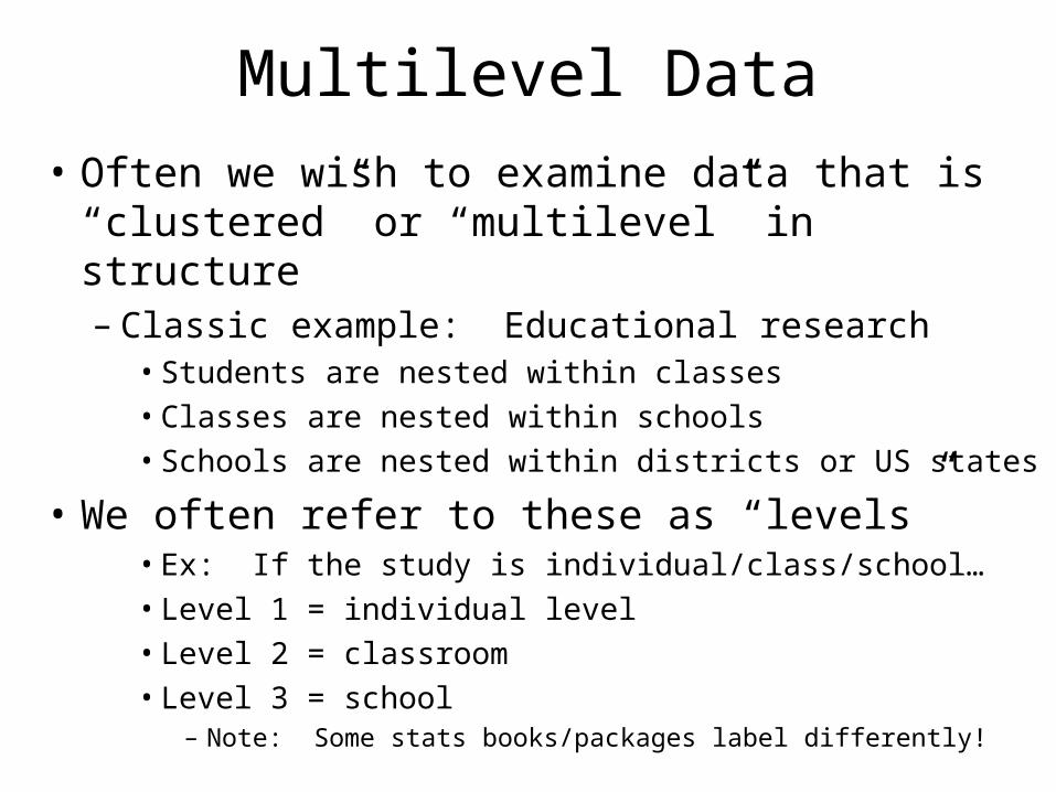
• Often we wish to examine data that is “clustered” or “multilevel” in structure– Classic example: Educational research

• Students are nested within classes• Classes are nested within schools• Schools are nested within districts or US states

• We often refer to these as “levels”• Ex: If the study is individual/class/school…• Level 1 = individual level• Level 2 = classroom• Level 3 = school

– Note: Some stats books/packages label differently!

Multilevel Data

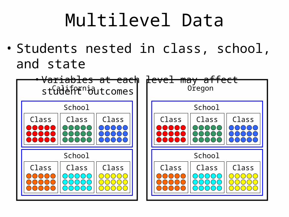
• Students nested in class, school, and state• Variables at each level may affect student outcomes

Class Class Class

School

Class Class Class

School

California

Class Class Class

School

Class Class Class

School

Oregon

Multilevel Data

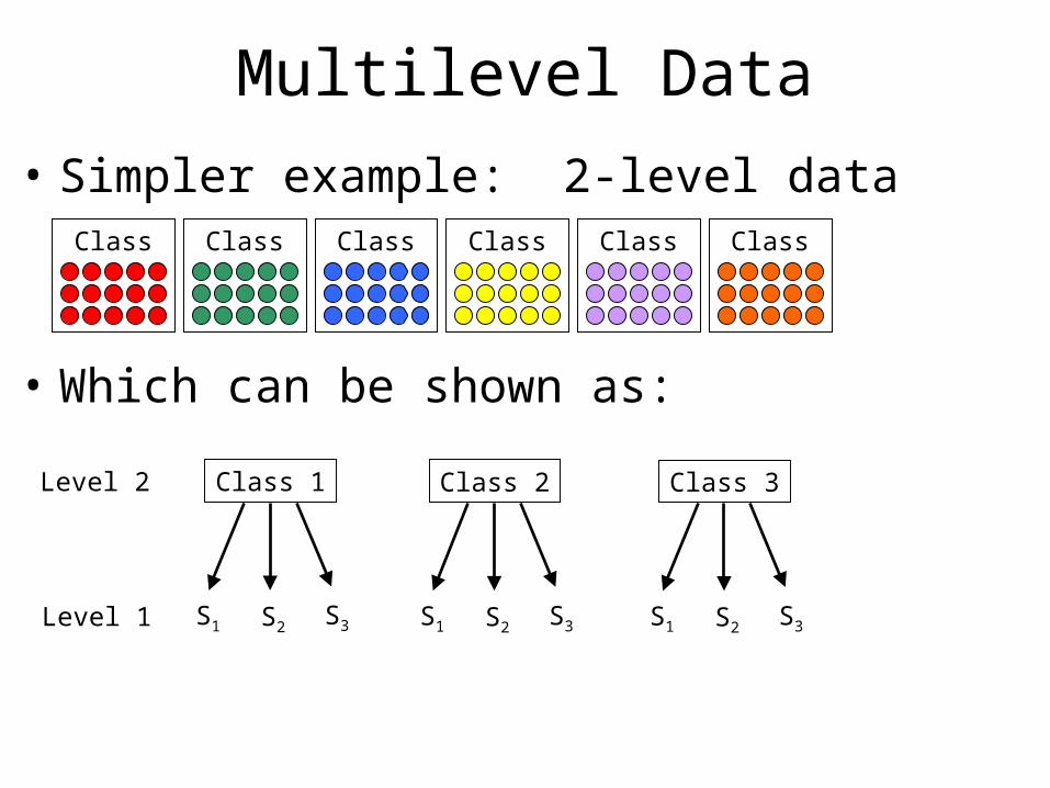
• Simpler example: 2-level dataClass Class Class Class Class Class

• Which can be shown as:

Class 1

S1 S2 S3

Class 2

S1 S2 S3

Class 3

S1 S2 S3

Level 2

Level 1

Multilevel Data

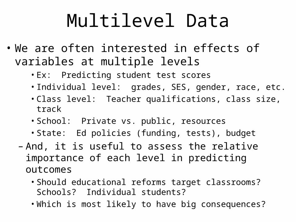
• We are often interested in effects of variables at multiple levels

• Ex: Predicting student test scores• Individual level: grades, SES, gender, race, etc.• Class level: Teacher qualifications, class size, track• School: Private vs. public, resources• State: Ed policies (funding, tests), budget

– And, it is useful to assess the relative importance of each level in predicting outcomes

• Should educational reforms target classrooms? Schools? Individual students?

• Which is most likely to have big consequences?

Multilevel Data

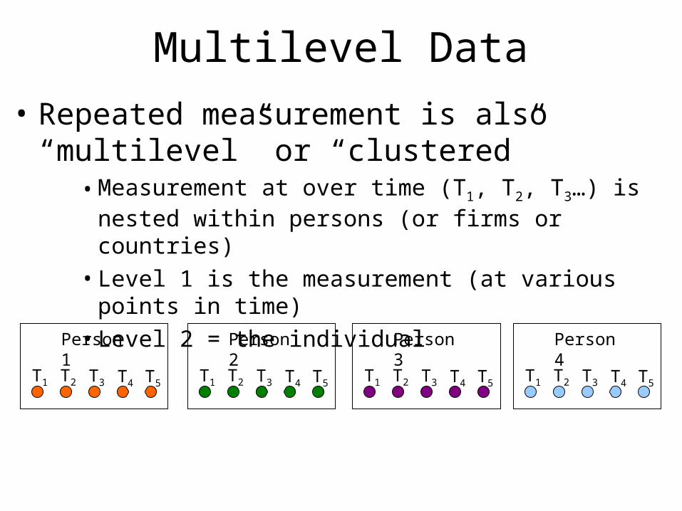
• Repeated measurement is also “multilevel” or “clustered”

• Measurement at over time (T1, T2, T3…) is nested within persons (or firms or countries)

• Level 1 is the measurement (at various points in time)• Level 2 = the individual

Person 1

T2T1 T4T3 T5

Person 2

T2T1 T4T3 T5

Person 3

T2T1 T4T3 T5

Person 4

T2T1 T4T3 T5

Multilevel Data

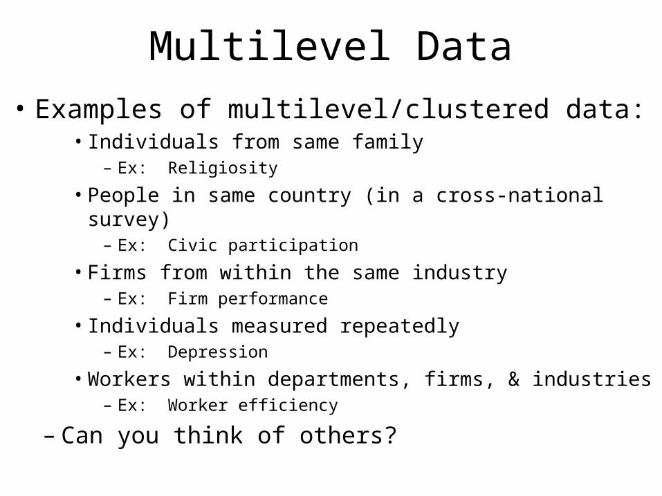
• Examples of multilevel/clustered data:• Individuals from same family

– Ex: Religiosity

• People in same country (in a cross-national survey)– Ex: Civic participation

• Firms from within the same industry– Ex: Firm performance

• Individuals measured repeatedly– Ex: Depression

• Workers within departments, firms, & industries– Ex: Worker efficiency

– Can you think of others?

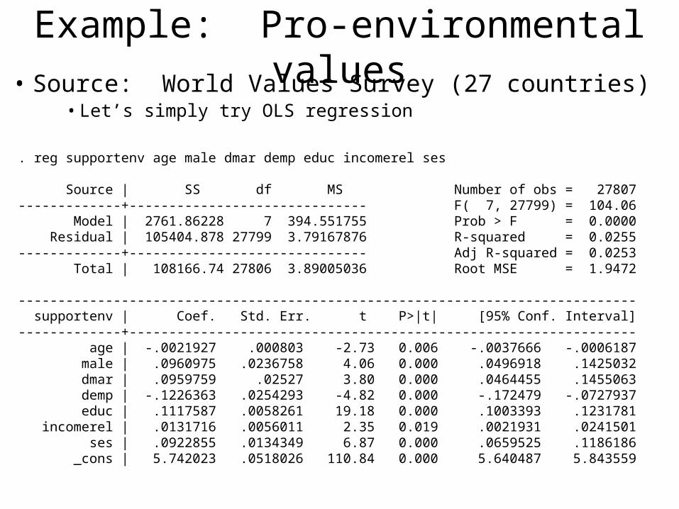
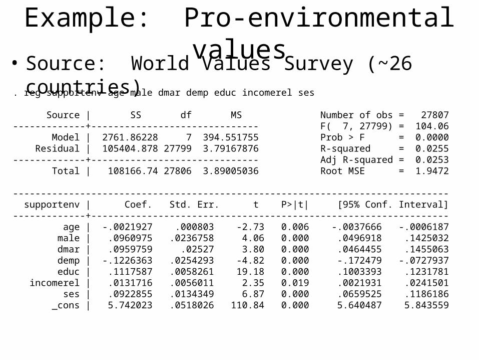
Example: Pro-environmental values• Source: World Values Survey (27 countries)

• Let’s simply try OLS regression

. reg supportenv age male dmar demp educ incomerel ses

Source | SS df MS Number of obs = 27807-------------+------------------------------ F( 7, 27799) = 104.06 Model | 2761.86228 7 394.551755 Prob > F = 0.0000 Residual | 105404.878 27799 3.79167876 R-squared = 0.0255-------------+------------------------------ Adj R-squared = 0.0253 Total | 108166.74 27806 3.89005036 Root MSE = 1.9472

------------------------------------------------------------------------------ supportenv | Coef. Std. Err. t P>|t| [95% Conf. Interval]-------------+---------------------------------------------------------------- age | -.0021927 .000803 -2.73 0.006 -.0037666 -.0006187 male | .0960975 .0236758 4.06 0.000 .0496918 .1425032 dmar | .0959759 .02527 3.80 0.000 .0464455 .1455063 demp | -.1226363 .0254293 -4.82 0.000 -.172479 -.0727937 educ | .1117587 .0058261 19.18 0.000 .1003393 .1231781 incomerel | .0131716 .0056011 2.35 0.019 .0021931 .0241501 ses | .0922855 .0134349 6.87 0.000 .0659525 .1186186 _cons | 5.742023 .0518026 110.84 0.000 5.640487 5.843559

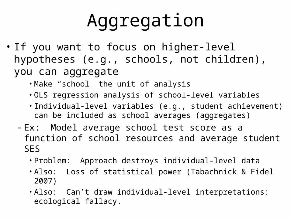
Aggregation

• If you want to focus on higher-level hypotheses (e.g., schools, not children), you can aggregate

• Make “school” the unit of analysis• OLS regression analysis of school-level variables• Individual-level variables (e.g., student achievement) can

be included as school averages (aggregates)

– Ex: Model average school test score as a function of school resources and average student SES

• Problem: Approach destroys individual-level data• Also: Loss of statistical power (Tabachnick & Fidel 2007)• Also: Can’t draw individual-level interpretations:

ecological fallacy.

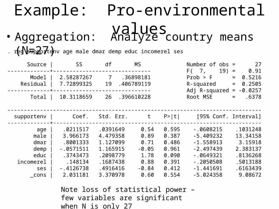
Example: Pro-environmental values• Aggregation: Analyze country means (N=27). reg supportenv age male dmar demp educ incomerel ses

Source | SS df MS Number of obs = 27-------------+------------------------------ F( 7, 19) = 0.91 Model | 2.58287267 7 .36898181 Prob > F = 0.5216 Residual | 7.72899325 19 .406789119 R-squared = 0.2505-------------+------------------------------ Adj R-squared = -0.0257 Total | 10.3118659 26 .396610228 Root MSE = .6378

------------------------------------------------------------------------------ supportenv | Coef. Std. Err. t P>|t| [95% Conf. Interval]-------------+---------------------------------------------------------------- age | .0211517 .0391649 0.54 0.595 -.0608215 .1031248 male | 3.966173 4.479358 0.89 0.387 -5.409232 13.34158 dmar | .8001333 1.127099 0.71 0.486 -1.558913 3.15918 demp | -.0571511 1.165915 -0.05 0.961 -2.497439 2.383137 educ | .3743473 .2098779 1.78 0.090 -.0649321 .8136268 incomerel | .148134 .1687438 0.88 0.391 -.2050508 .5013188 ses | -.4126738 .4916416 -0.84 0.412 -1.441691 .6163439 _cons | 2.031181 3.370978 0.60 0.554 -5.024358 9.08672

Note loss of statistical power – few variables are significant when N is only 27

Ecological Fallacy• Issue: Data aggregation limits your ability to

draw conclusions about level-1 units• The “ecological fallacy”

– Robinson, W.S. (1950). "Ecological Correlations and the Behavior of Individuals". American Sociological Review 15: 351–357

• Among US states, immigration rate correlates positively with average literacy

• Does this mean that immigrants tend to be more literate than US citizens?

• NO: You can’t assume an individual-level correlation!– The correlation at individual level is actually negative– But: immigrants settled in states with high levels of literacy –

yielding a correlation in aggregate statistics.

OLS Approaches

• Another option: Just use OLS regression• Allows you to focus on lower-level units

– No need for aggregation

• Ex: Just analyze individuals as the unit of analysis, ignoring clustering among schools

• Include independent variables measured at the individual-level and other levels

• Problems:• 1. Violates OLS assumptions (see below)• 2. OLS is too limited; can’t take advantage of richness of

multilevel data– Ex: Complex variation in intercepts, slopes across groups.

Multilevel Data: Problems

• Issue: Multilevel data often results in violation of OLS regression assumption

• OLS requires an independent random sample…• Students from the same class (or school) are not

independent… and may have correlated error

– If you don’t control for sources of correlated error, models tend to underestimate standard errors

• This leads to false rejection of H0– Too many asterisks in table (Type I error)

• This is a serious issue, as we always want to err in the direction of conservatism… false findings = bad!

Multilevel Data: Problems• Why might nested data have correlated error?

– Example: Student performance on a test• Students in a given classroom may share & experience

common (unobserved) characteristics• Ex: Maybe the classroom is too dark, causing all

students to perform poorly on tests

– If all those students score poorly, they fall below the regression line… and have negative error

– But OLS regression requires that error be “random”– Within-class error should be random, not consistently negative

– Other sources of within-class (or school) error• An especially good teacher; poor school funding• Other ideas?

Multilevel Data: Problems

• Sources of correlated error within groups– Ex: Cross-national study of homelessness

• People in welfare states have a common unobserved characteristic: access to generous benefits

– Ex: Study of worker efficiency in workgroups• Group members may influence each other (peer

pressure) leading to group commonalities.

Multilevel Data: Problems

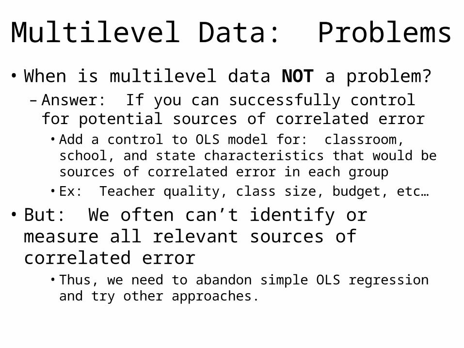
• When is multilevel data NOT a problem?– Answer: If you can successfully control for

potential sources of correlated error• Add a control to OLS model for: classroom, school,

and state characteristics that would be sources of correlated error in each group

• Ex: Teacher quality, class size, budget, etc…

• But: We often can’t identify or measure all relevant sources of correlated error

• Thus, we need to abandon simple OLS regression and try other approaches.

Example: Pro-environmental values• Source: World Values Survey (~26 countries). reg supportenv age male dmar demp educ incomerel ses

Source | SS df MS Number of obs = 27807-------------+------------------------------ F( 7, 27799) = 104.06 Model | 2761.86228 7 394.551755 Prob > F = 0.0000 Residual | 105404.878 27799 3.79167876 R-squared = 0.0255-------------+------------------------------ Adj R-squared = 0.0253 Total | 108166.74 27806 3.89005036 Root MSE = 1.9472

------------------------------------------------------------------------------ supportenv | Coef. Std. Err. t P>|t| [95% Conf. Interval]-------------+---------------------------------------------------------------- age | -.0021927 .000803 -2.73 0.006 -.0037666 -.0006187 male | .0960975 .0236758 4.06 0.000 .0496918 .1425032 dmar | .0959759 .02527 3.80 0.000 .0464455 .1455063 demp | -.1226363 .0254293 -4.82 0.000 -.172479 -.0727937 educ | .1117587 .0058261 19.18 0.000 .1003393 .1231781 incomerel | .0131716 .0056011 2.35 0.019 .0021931 .0241501 ses | .0922855 .0134349 6.87 0.000 .0659525 .1186186 _cons | 5.742023 .0518026 110.84 0.000 5.640487 5.843559

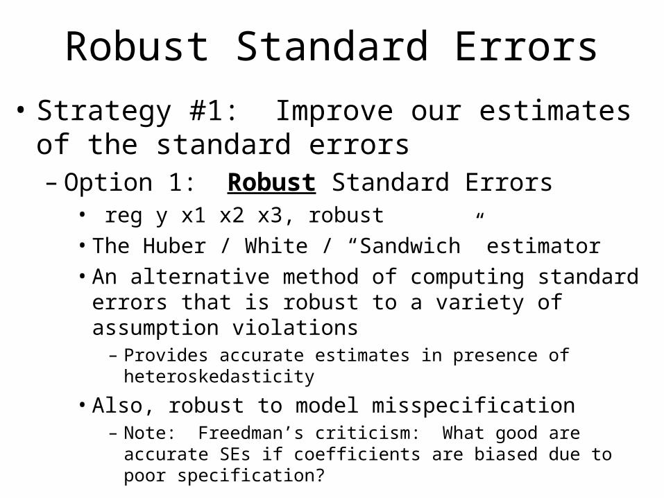
Robust Standard Errors

• Strategy #1: Improve our estimates of the standard errors– Option 1: Robust Standard Errors

• reg y x1 x2 x3, robust• The Huber / White / “Sandwich” estimator• An alternative method of computing standard errors

that is robust to a variety of assumption violations– Provides accurate estimates in presence of heteroskedasticity

• Also, robust to model misspecification– Note: Freedman’s criticism: What good are accurate SEs if

coefficients are biased due to poor specification?

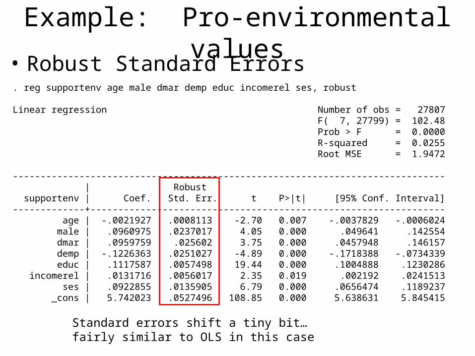
Example: Pro-environmental values• Robust Standard Errors. reg supportenv age male dmar demp educ incomerel ses, robust

Linear regression Number of obs = 27807 F( 7, 27799) = 102.48 Prob > F = 0.0000 R-squared = 0.0255 Root MSE = 1.9472

------------------------------------------------------------------------------ | Robust supportenv | Coef. Std. Err. t P>|t| [95% Conf. Interval]-------------+---------------------------------------------------------------- age | -.0021927 .0008113 -2.70 0.007 -.0037829 -.0006024 male | .0960975 .0237017 4.05 0.000 .049641 .142554 dmar | .0959759 .025602 3.75 0.000 .0457948 .146157 demp | -.1226363 .0251027 -4.89 0.000 -.1718388 -.0734339 educ | .1117587 .0057498 19.44 0.000 .1004888 .1230286 incomerel | .0131716 .0056017 2.35 0.019 .002192 .0241513 ses | .0922855 .0135905 6.79 0.000 .0656474 .1189237 _cons | 5.742023 .0527496 108.85 0.000 5.638631 5.845415

Standard errors shift a tiny bit… fairly similar to OLS in this case

Robust Cluster Standard Errors

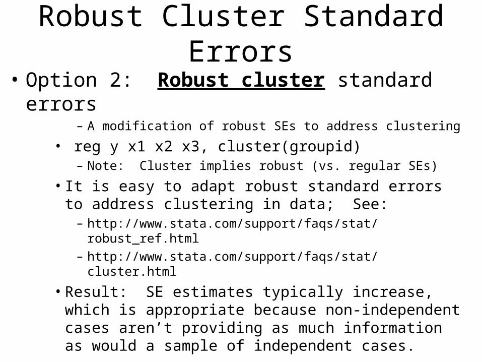
• Option 2: Robust cluster standard errors– A modification of robust SEs to address clustering

• reg y x1 x2 x3, cluster(groupid)– Note: Cluster implies robust (vs. regular SEs)

• It is easy to adapt robust standard errors to address clustering in data; See:

– http://www.stata.com/support/faqs/stat/robust_ref.html– http://www.stata.com/support/faqs/stat/cluster.html

• Result: SE estimates typically increase, which is appropriate because non-independent cases aren’t providing as much information as would a sample of independent cases.

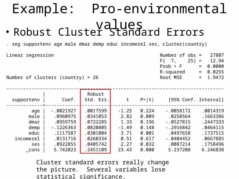
Example: Pro-environmental values• Robust Cluster Standard Errors. reg supportenv age male dmar demp educ incomerel ses, cluster(country)

Linear regression Number of obs = 27807 F( 7, 25) = 12.94 Prob > F = 0.0000 R-squared = 0.0255Number of clusters (country) = 26 Root MSE = 1.9472

------------------------------------------------------------------------------ | Robust supportenv | Coef. Std. Err. t P>|t| [95% Conf. Interval]-------------+---------------------------------------------------------------- age | -.0021927 .0017599 -1.25 0.224 -.0058172 .0014319 male | .0960975 .0341053 2.82 0.009 .0258564 .1663386 dmar | .0959759 .0722285 1.33 0.196 -.0527815 .2447333 demp | -.1226363 .0820805 -1.49 0.148 -.2916842 .0464115 educ | .1117587 .0301004 3.71 0.001 .0497658 .1737515 incomerel | .0131716 .0260334 0.51 0.617 -.0404452 .0667885 ses | .0922855 .0405742 2.27 0.032 .0087214 .1758496 _cons | 5.742023 .2451109 23.43 0.000 5.237208 6.246838

Cluster standard errors really change the picture. Several variables lose statistical significance.

Dummy Variables

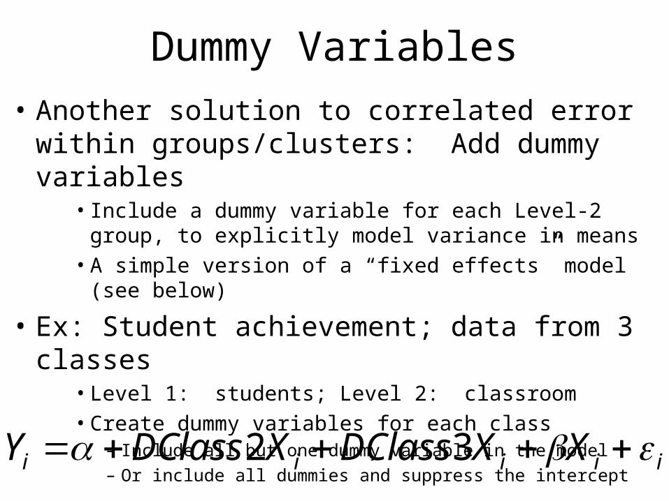
• Another solution to correlated error within groups/clusters: Add dummy variables

• Include a dummy variable for each Level-2 group, to explicitly model variance in means

• A simple version of a “fixed effects” model (see below)

• Ex: Student achievement; data from 3 classes• Level 1: students; Level 2: classroom• Create dummy variables for each class

– Include all but one dummy variable in the model– Or include all dummies and suppress the intercept

iiiii XXDClassXDClassY 32

Dummy Variables

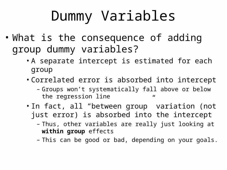
• What is the consequence of adding group dummy variables?

• A separate intercept is estimated for each group• Correlated error is absorbed into intercept

– Groups won’t systematically fall above or below the regression line

• In fact, all “between group” variation (not just error) is absorbed into the intercept

– Thus, other variables are really just looking at within group effects

– This can be good or bad, depending on your goals.

Dummy Variables

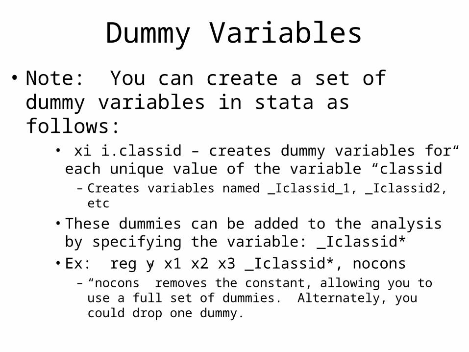
• Note: You can create a set of dummy variables in stata as follows:

• xi i.classid – creates dummy variables for each unique value of the variable “classid”

– Creates variables named _Iclassid_1, _Iclassid2, etc

• These dummies can be added to the analysis by specifying the variable: _Iclassid*

• Ex: reg y x1 x2 x3 _Iclassid*, nocons – “nocons” removes the constant, allowing you to use a full set

of dummies. Alternately, you could drop one dummy.

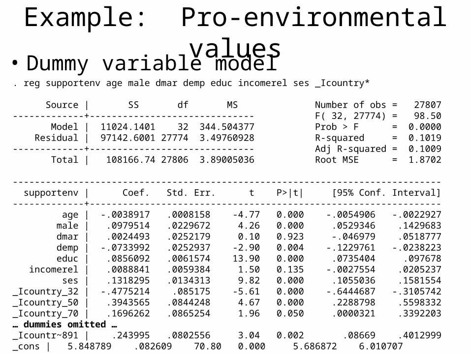
Example: Pro-environmental values• Dummy variable model. reg supportenv age male dmar demp educ incomerel ses _Icountry*

Source | SS df MS Number of obs = 27807-------------+------------------------------ F( 32, 27774) = 98.50 Model | 11024.1401 32 344.504377 Prob > F = 0.0000 Residual | 97142.6001 27774 3.49760928 R-squared = 0.1019-------------+------------------------------ Adj R-squared = 0.1009 Total | 108166.74 27806 3.89005036 Root MSE = 1.8702

------------------------------------------------------------------------------ supportenv | Coef. Std. Err. t P>|t| [95% Conf. Interval]-------------+---------------------------------------------------------------- age | -.0038917 .0008158 -4.77 0.000 -.0054906 -.0022927 male | .0979514 .0229672 4.26 0.000 .0529346 .1429683 dmar | .0024493 .0252179 0.10 0.923 -.046979 .0518777 demp | -.0733992 .0252937 -2.90 0.004 -.1229761 -.0238223 educ | .0856092 .0061574 13.90 0.000 .0735404 .097678 incomerel | .0088841 .0059384 1.50 0.135 -.0027554 .0205237 ses | .1318295 .0134313 9.82 0.000 .1055036 .1581554_Icountry_32 | -.4775214 .085175 -5.61 0.000 -.6444687 -.3105742_Icountry_50 | .3943565 .0844248 4.67 0.000 .2288798 .5598332_Icountry_70 | .1696262 .0865254 1.96 0.050 .0000321 .3392203… dummies omitted … _Icountr~891 | .243995 .0802556 3.04 0.002 .08669 .4012999_cons | 5.848789 .082609 70.80 0.000 5.686872 6.010707

Dummy Variables• Benefits of the dummy variable approach

• It is simple – Just estimate a different intercept for each group

• sometimes the dummy interpretations can be of interest

• Weaknesses• Cumbersome if you have many groups• Uses up lots of degrees of freedom (not parsimonious)• Makes it hard to look at other kinds of group dummies

– Non-varying group variables = collinear with dummies

• Can be problematic if your main interest is to study effects of variables across groups

– Dummies purge that variation… focus on within-group variation

– If you don’t have much within group variation, there isn’t much left to analyze.

Dummy Variables

• Note: Dummy variables are a simple example of a “fixed effects” model (FEM)

• Effect of each group is modeled as a “fixed effect” rather than a random variable

• Also can be thought of as the “within-group” estimator– Looks purely at variation within groups

– Stata can do a Fixed Effects Model without the effort of using all the dummy variables

• Simply request the “fixed effects” estimator in xtreg.

Fixed Effects Model (FEM)

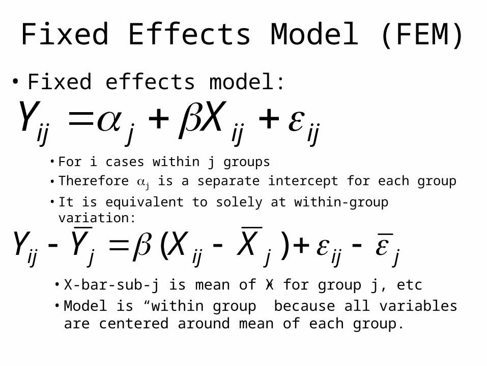
• Fixed effects model:

ijijjij XY • For i cases within j groups

• Therefore j is a separate intercept for each group

• It is equivalent to solely at within-group variation:

jijjijjij XXYY )(• X-bar-sub-j is mean of X for group j, etc• Model is “within group” because all variables are

centered around mean of each group.

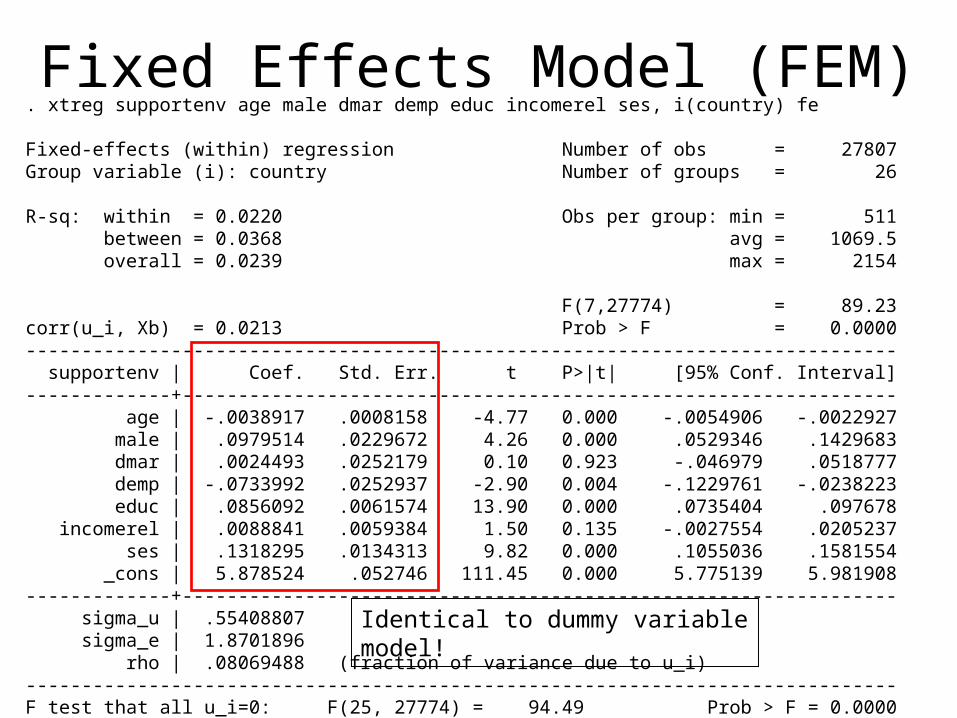
Fixed Effects Model (FEM). xtreg supportenv age male dmar demp educ incomerel ses, i(country) fe

Fixed-effects (within) regression Number of obs = 27807Group variable (i): country Number of groups = 26

R-sq: within = 0.0220 Obs per group: min = 511 between = 0.0368 avg = 1069.5 overall = 0.0239 max = 2154

F(7,27774) = 89.23corr(u_i, Xb) = 0.0213 Prob > F = 0.0000------------------------------------------------------------------------------ supportenv | Coef. Std. Err. t P>|t| [95% Conf. Interval]-------------+---------------------------------------------------------------- age | -.0038917 .0008158 -4.77 0.000 -.0054906 -.0022927 male | .0979514 .0229672 4.26 0.000 .0529346 .1429683 dmar | .0024493 .0252179 0.10 0.923 -.046979 .0518777 demp | -.0733992 .0252937 -2.90 0.004 -.1229761 -.0238223 educ | .0856092 .0061574 13.90 0.000 .0735404 .097678 incomerel | .0088841 .0059384 1.50 0.135 -.0027554 .0205237 ses | .1318295 .0134313 9.82 0.000 .1055036 .1581554 _cons | 5.878524 .052746 111.45 0.000 5.775139 5.981908-------------+---------------------------------------------------------------- sigma_u | .55408807 sigma_e | 1.8701896 rho | .08069488 (fraction of variance due to u_i)------------------------------------------------------------------------------F test that all u_i=0: F(25, 27774) = 94.49 Prob > F = 0.0000

Identical to dummy variable model!