multilevel analysis of spatiotemporal association...
TRANSCRIPT
Multilevel analysis of spatiotemporal association features for differentiationof tumor enhancement patterns in breast DCE-MRI
Sang Ho LeeInterdisciplinary Program in Radiation Applied Life Science, Seoul National University College ofMedicine, and Institute of Radiation Medicine, Seoul National University Medical Research Center,Seoul 110-744, Korea
Jong Hyo Kima�
Department of Radiology, Seoul National University College of Medicine, Seoul 110-744, Korea
Nariya Cho and Jeong Seon Parkb�
Department of Radiology, Seoul National University Hospital, Seoul 110-744, Korea
Zepa YangDepartment of Biomedical Sciences, Seoul National University College of Medicine, Seoul 110-744, Korea
Yun Sub JungInterdisciplinary Program in Radiation Applied Life Science, Seoul National University College ofMedicine, Seoul 110-744, Korea
Woo Kyung MoonDepartment of Radiology, Seoul National University College of Medicine, Seoul, 110-744, Korea
�Received 17 November 2009; revised 1 April 2010; accepted for publication 5 May 2010;published 12 July 2010�
Purpose: Analyzing spatiotemporal enhancement patterns is an important task for the differentialdiagnosis of breast tumors in dynamic contrast-enhanced MRI �DCE-MRI�, and yet remains chal-lenging because of complexities in analyzing the time-series of three-dimensional image data. Theauthors propose a novel approach to breast MRI computer-aided diagnosis �CAD� using a multi-level analysis of spatiotemporal association features for tumor enhancement patterns in DCE-MRI.Methods: A database of 171 cases consisting of 111 malignant and 60 benign tumors was used.Time-series contrast-enhanced MR images were obtained from two different types of MR scannersand protocols. The images were first registered for motion compensation, and then tumor regionswere segmented using a fuzzy c-means clustering-based method. Spatiotemporal associations oftumor enhancement patterns were analyzed at three levels: Mapping of pixelwise kinetic featureswithin a tumor, extraction of spatial association features from kinetic feature maps, and extractionof kinetic association features at the spatial feature level. A total of 84 initial features were ex-tracted. Predictable values of these features were evaluated with an area under the ROC curve, andwere compared between the spatiotemporal association features and a subset of simple form fea-tures which do not reflect spatiotemporal association. Several optimized feature sets were identifiedamong the spatiotemporal association feature group or among the simple feature group based on afeature ranking criterion using a support vector machine based recursive feature elimination algo-rithm. A least-squares support vector machine �LS-SVM� classifier was used for tumor differentia-tion and the performances were evaluated using a leave-one-out testing.Results: Predictable values of the extracted single features ranged in 0.52–0.75. By applyingmultilevel analysis strategy, the spatiotemporal association features became more informative inpredicting tumor malignancy, which was shown by a statistical testing in ten spatiotemporal asso-ciation features. By using a LS-SVM classifier with the optimized second and third level feature set,the CAD scheme showed Az of 0.88 in classification of malignant and benign tumors. When thisperformance was compared to the same LS-SVM classifier with simple form features which do notreflect spatiotemporal association, there was a statistically significant difference �0.88 vs 0.79, p�0.05�, suggesting that the multilevel analysis strategy yields a significant performance improve-ment.Conclusions: The results suggest that the multilevel analysis strategy characterizes the complextumor enhancement patterns effectively with the spatiotemporal association features, which in turnleads to an improved tumor differentiation. The proposed CAD scheme has a potential for improv-ing diagnostic performance in breast DCE-MRI. © 2010 American Association of Physicists in
Medicine. �DOI: 10.1118/1.3446799�3940 3940Med. Phys. 37 „8…, August 2010 0094-2405/2010/37„8…/3940/17/$30.00 © 2010 Am. Assoc. Phys. Med.

3941 Lee et al.: Spatiotemporal association features for MR-based breast tumor diagnosis 3941
Key words: breast dynamic contrast-enhanced MRI, computer-aided diagnosis, spatiotemporalassociation, feature extraction, classification, 3D moment invariants, support vector machines, tu-mor characterization
I. INTRODUCTION
Dynamic contrast-enhanced �DCE� breast MRI is being ap-plied for detection, diagnosis, and staging of breast cancer.As breast DCE-MRI is recently recommended as a screeningoption of breast cancer for women at high risk,1–6 differen-tiation of malignant and benign tumors is becoming a moreimportant function in breast DCE-MRI.
The breast DCE-MRI produces a high spatial resolutionand time course imaging data on contrast enhancements of atumor and its surrounding tissue. The abundance of informa-tion it provides is potentially capable of differentiation be-tween malignant and benign tumors.7
In principle, the contrast enhancement kinetics and mor-phological features in breast DCE-MRI provide valuable in-formation for diagnosing suspected malignancy of breasttumors.8 Previous studies have reported the efficacy of con-trast enhancement kinetics in evaluating tumor vasculariza-tion, which has been correlated with biological and clinicalaggressiveness.9,10 The differences in tumor vascularitypresent varying degrees of contrast enhancement patterns inDCE-MRI according to their malignancy; malignant lesionstypically exhibit early strong enhancement with rapid wash-out, whereas benign lesions usually show a slow increasefollowed by persistent enhancement.9 Morphological criteriahave also been verified as valuable diagnostic tools in differ-ential diagnosis of breast tumors.11,12 Spiculate margin, inter-nal heterogeneous or rim enhancement, and irregular shapeare important predictors of malignancy, whereas smoothmargin, internal homogeneous enhancement, and regularshape are related to benignancy in general.8
In conventional practice, kinetic and morphological fea-tures are evaluated in subjective ways. The majority of ki-netic analysis for breast tumors has been carried out onmanual placement of a region of interest �ROI� within atumor.9,13,14 Various morphological features are also evalu-ated in subjective ways based on observer experience. Al-though the Breast Imaging Reporting and Data System lexi-con provides useful criteria on visual assessment of varioustumor morphologies,15 priority and weights on different mor-phological features are not standardized. In addition, visualassessment of time-series image data containing complexspatiotemporal features by radiologists is a time consumingtask and imposes another impediment.
In order to overcome such limits, considerable effortshave been put on the development of computer-aided diag-nosis �CAD� algorithms. For objective classification of ki-netic features from the ROI, Lucht et al.16 applied artificialneural network and Levman et al.17 introduced support vec-tor machine �SVM�. For quantitative evaluation of morpho-logical features, Gilhuijs et al.18 employed radial gradienthistogram and other shape measures. Studies have also been
conducted to include both kinetic and morphological featuresMedical Physics, Vol. 37, No. 8, August 2010
in CAD schemes. Chen et al.19 analyzed dynamics of en-hancement variance within segmented tumors and Meinel etal.20 used backpropagation neural network to classify a com-bined set of shape and kinetic features from the segmentedtumor region. Recently, Zheng et al.21,22 applied discreteFourier transformation �DFT� to kinetic curves and extractedHu’s moment invariants from the DFT coefficients of se-lected two-dimensional images.
A major challenge in the diagnosis of breast DCE-MRI isto analyze the complexity on the spatiotemporal associationof tumor enhancement patterns. In fact, the morphologicalpattern of a tumor in DCE-MRI dynamically changes due todiverse time courses of signal enhancement at each pixel.Likewise, the kinetic patterns of enhancement are differenton various parts within a tumor. In most previous studies,however, the associations between spatial and temporal fea-tures were rarely investigated, and these features weretreated separately; the morphological features were extractedat a specific time point assuming they are fixed; when ex-tracting the kinetic features, their spatial dependency wasalso mostly neglected.
In this study, we postulate that analyzing spatiotemporalassociations of tumor enhancement patterns would gain ad-ditional information otherwise not attainable, and thus mayallow an improved performance for tumor differentiation.Based on this postulation, we propose a novel approach tobreast MRI CAD using multilevel analysis of spatiotemporalassociation features for tumor enhancement patterns inDCE-MR images.
II. MATERIALS AND METHODS
II.A. Patients
A total of 171 female patients �mean age, 46.7 yr�8�SD�; range, 25–74 yr� were included in this retrospectivestudy, from which one primary lesion per patient was usedfor analysis. All patients were seen in our radiology depart-ment for mammographic and/or sonographic abnormalitiesand underwent breast DCE-MRI at our institution betweenJanuary 2004 and December 2009.
Our database consisted of two data sets: Data set 1 of 75patients �mean age, 45.6 yr�8 �SD�; range, 25–61 yr�, ob-tained with a MR scanner 1 �Magnetom Sonata; Siemens,Erlangen, Germany� during January 2004 and December2006; and data set 2 of 96 patients �mean age, 47.5 yr�8�SD�; range, 32–74 yr�, obtained with a MR scanner 2 �Si-gna; GE Medical Systems, Milwaukee, WI� during January2007 to December 2009. As a total, our database contained111 malignant and 60 benign lesions. All malignant lesionsand 52 benign lesions were proved by histological examina-tion using surgically excised specimens and eight benign le-
sions were confirmed by core biopsies or follow-up exami-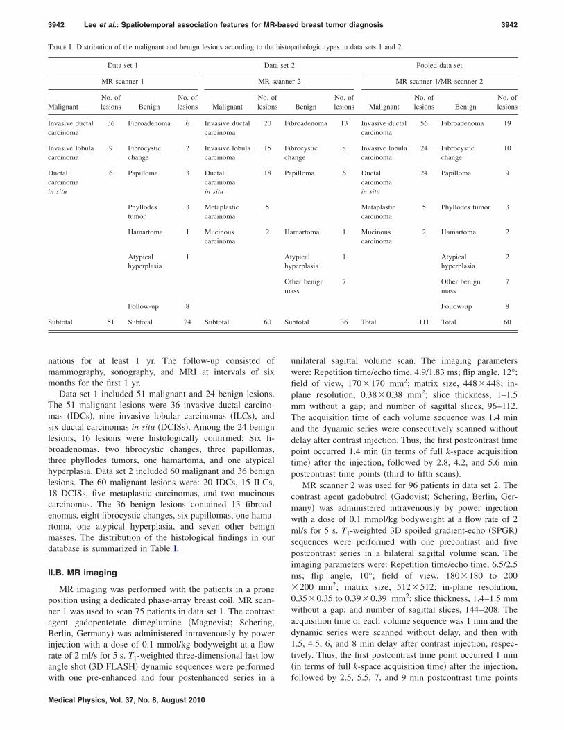
3942 Lee et al.: Spatiotemporal association features for MR-based breast tumor diagnosis 3942
nations for at least 1 yr. The follow-up consisted ofmammography, sonography, and MRI at intervals of sixmonths for the first 1 yr.
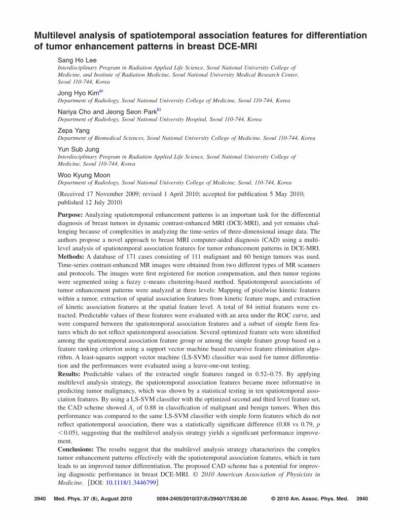
Data set 1 included 51 malignant and 24 benign lesions.The 51 malignant lesions were 36 invasive ductal carcino-mas �IDCs�, nine invasive lobular carcinomas �ILCs�, andsix ductal carcinomas in situ �DCISs�. Among the 24 benignlesions, 16 lesions were histologically confirmed: Six fi-broadenomas, two fibrocystic changes, three papillomas,three phyllodes tumors, one hamartoma, and one atypicalhyperplasia. Data set 2 included 60 malignant and 36 benignlesions. The 60 malignant lesions were: 20 IDCs, 15 ILCs,18 DCISs, five metaplastic carcinomas, and two mucinouscarcinomas. The 36 benign lesions contained 13 fibroad-enomas, eight fibrocystic changes, six papillomas, one hama-rtoma, one atypical hyperplasia, and seven other benignmasses. The distribution of the histological findings in ourdatabase is summarized in Table I.
II.B. MR imaging
MR imaging was performed with the patients in a proneposition using a dedicated phase-array breast coil. MR scan-ner 1 was used to scan 75 patients in data set 1. The contrastagent gadopentetate dimeglumine �Magnevist; Schering,Berlin, Germany� was administered intravenously by powerinjection with a dose of 0.1 mmol/kg bodyweight at a flowrate of 2 ml/s for 5 s. T1-weighted three-dimensional fast lowangle shot �3D FLASH� dynamic sequences were performed
TABLE I. Distribution of the malignant and benign lesions according to the
Data set 1 Data
MR scanner 1 MR s
MalignantNo. oflesions Benign
No. oflesions Malignant
No. oflesions
Invasive ductalcarcinoma
36 Fibroadenoma 6 Invasive ductalcarcinoma
20
Invasive lobulacarcinoma
9 Fibrocysticchange
2 Invasive lobulacarcinoma
15
Ductalcarcinomain situ
6 Papilloma 3 Ductalcarcinomain situ
18
Phyllodestumor
3 Metaplasticcarcinoma
5
Hamartoma 1 Mucinouscarcinoma
2
Atypicalhyperplasia
1
Follow-up 8
Subtotal 51 Subtotal 24 Subtotal 60
with one pre-enhanced and four postenhanced series in a
Medical Physics, Vol. 37, No. 8, August 2010
unilateral sagittal volume scan. The imaging parameterswere: Repetition time/echo time, 4.9/1.83 ms; flip angle, 12°;field of view, 170�170 mm2; matrix size, 448�448; in-plane resolution, 0.38�0.38 mm2; slice thickness, 1–1.5mm without a gap; and number of sagittal slices, 96–112.The acquisition time of each volume sequence was 1.4 minand the dynamic series were consecutively scanned withoutdelay after contrast injection. Thus, the first postcontrast timepoint occurred 1.4 min �in terms of full k-space acquisitiontime� after the injection, followed by 2.8, 4.2, and 5.6 minpostcontrast time points �third to fifth scans�.
MR scanner 2 was used for 96 patients in data set 2. Thecontrast agent gadobutrol �Gadovist; Schering, Berlin, Ger-many� was administered intravenously by power injectionwith a dose of 0.1 mmol/kg bodyweight at a flow rate of 2ml/s for 5 s. T1-weighted 3D spoiled gradient-echo �SPGR�sequences were performed with one precontrast and fivepostcontrast series in a bilateral sagittal volume scan. Theimaging parameters were: Repetition time/echo time, 6.5/2.5ms; flip angle, 10°; field of view, 180�180 to 200�200 mm2; matrix size, 512�512; in-plane resolution,0.35�0.35 to 0.39�0.39 mm2; slice thickness, 1.4–1.5 mmwithout a gap; and number of sagittal slices, 144–208. Theacquisition time of each volume sequence was 1 min and thedynamic series were scanned without delay, and then with1.5, 4.5, 6, and 8 min delay after contrast injection, respec-tively. Thus, the first postcontrast time point occurred 1 min�in terms of full k-space acquisition time� after the injection,
athologic types in data sets 1 and 2.
2 Pooled data set
r 2 MR scanner 1/MR scanner 2
BenignNo. oflesions Malignant
No. oflesions Benign
No. oflesions
broadenoma 13 Invasive ductalcarcinoma
56 Fibroadenoma 19
brocysticange
8 Invasive lobulacarcinoma
24 Fibrocysticchange
10
pilloma 6 Ductalcarcinomain situ
24 Papilloma 9
Metaplasticcarcinoma
5 Phyllodes tumor 3
martoma 1 Mucinouscarcinoma
2 Hamartoma 2
ypicalperplasia
1 Atypicalhyperplasia
2
her benignss
7 Other benignmass
7
Follow-up 8
btotal 36 Total 111 Total 60
histop
set
canne
Fi
Fich
Pa
Ha
Athy
Otma
Su
followed by 2.5, 5.5, 7, and 9 min postcontrast time points
3943 Lee et al.: Spatiotemporal association features for MR-based breast tumor diagnosis 3943
�third to sixth scans�. Details of the two different MR imag-ing protocols used in the analysis are summarized in Table II.
II.C. Image registration
In order to reduce possible artifacts or blurring due to thepatient motion, we aligned all postcontrast series to the pre-contrast one �first series� of the dynamic sequences using a3D rigid registration technique based on the maximization ofmutual information.23 The registered MR images were visu-ally inspected and evaluated by two experienced and highlytrained radiologists in consensus and confirmed to be helpfulfor motion compensation.
II.D. Tumor segmentation
For breast tumor segmentation on DCE-MR images, abox-shaped 3D volume of interest �VOI� was selected tocontain the lesion by a human operator for each case. Thesize of a rectangle bounding the lesion in each slice level wasdetermined by the largest extent of the lesion shown in arepresentative middle slice. And then, a fuzzy c-means�FCM� clustering algorithm was applied to segment tumorout of background tissue.24,25 While FCM clustering wasusually performed using vector data to represent time-seriesdata in previous studies, we employed a scalar value in thisstudy that extract more compact information from all time-series data in order to be better applicable to our two datasets having different temporal acquisition protocols.
A scalar signal, denoted as variance of enhancement slope�VES�, was used to represent the pharmacokinetic activity ateach pixel.26 The VES is given as the following expression:
VES = Var� It − I0
t�, 0 � t � M , �1�
where t denotes the time elapsed �min� from contrast injec-
TABLE II. MR imaging protocols used for image acq
Imaging parameter M
Contrast agent GadopenDose �mmol/kg�
Injection rate �ml/s�Injection duration �s�B0 field strength �T�
Pulse sequence T1-weiScan coverage
PlaneTR/TE �ms�
Flip angle �deg�Field of view �mm2�Matrix size �pixel�
In-plane resolution �mm2�Slice thickness �mm�
No. of slices/gap 9Volume scan time �min�
Dynamic acquisition time �min� 1.4No. of postcontrast series
tion and M is the elapsed time of the last temporal phase,
Medical Physics, Vol. 37, No. 8, August 2010
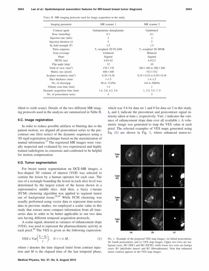
which was 5.6 for data set 1 and 9 for data set 2 in this study.I0 and It indicate the precontrast and postcontrast signal in-tensity taken at time t, respectively. Var� · � indicates the vari-ance of enhancement slope data over all available t. A volu-metric image was generated to map the VES value at eachpixel. The selected examples of VES maps generated usingEq. �1� are shown in Fig. 1, where enhanced tumor-to-
on in the study.
anner 1 MR scanner 2
dimeglumine Gadobutrol.1 0.1
25
.5 1.53D FLASH T1-weighted 3D SPGRteral Bilateral
ittal Sagittal1.83 6.5/2.52 10
170 180�180 to 200�200448 512�5120.38 0.35�0.35 to 0.39�0.39
1.5 1.4–1.512/No 144 to 208/No
.4 14.2, 5.6 1, 2.5, 5.5, 7, 9
5
FIG. 1. Example of the proposed VES map images: �a� Initial postcontrast,�b� fourth postcontrast, and �c� VES map images. Upper two rows are ma-lignant cases: M1 �IDC� and M2 �DCIS�, while lower two rows are benigncases: B1 �phyllodes tumor� and B2 �fibroadenoma�. Note that enhanced
uisiti
R sc
tetate025
1ghtedUnilaSag4.9/
1170�
448�
0.38�
1–6 to 1
1, 2.8,
4
tumor contrast appears in the VES map images.
3944 Lee et al.: Spatiotemporal association features for MR-based breast tumor diagnosis 3944
parenchyma contrast is demonstrated in both malignant andbenign cases.
The FCM clustering algorithm is a fuzzy equivalent to the“hard” k-means clustering, where the assignment of fuzzymembership values can serve as a confidence measure intumor segmentation. Let X= �xi , i=1,2 , ¯ ,N �xi�R denotethe input data set compromising N pixels to be partitionedinto c clusters. In this study, the data point xi was the scalarvalue of VES at pixel i within the 3D VOI. The FCM clus-tering was applied to partition the VOI pixels into two cat-egories �c=2�: Tumor and background parenchyma. Fuzzypartitioning for breast tumor segmentation was carried outthrough an iterative optimization to minimize the within-group error function J defined as
J = k=1
2
i=1
N
uki2 �xi − vk�2, �2�
with the following constraints:
k=1
2
uki = 1, ∀ i;0 � uki � 1, ∀ k,
i;i=1
N
uki � 0, ∀ k , �3�
where N is the number of pixels in the 3D VOI, ukj is themembership probability that xi belongs to cluster k, vk is thekth cluster center obtained from weighted averaging of xi,and � · � denotes the Euclidean distance expressing the simi-larity between any measured data and the center, respec-tively. The within-group error function J is minimized whenhigh membership values are assigned to the pixels close tothe centroids of clusters, and low membership values to thepixels far from the centroids. The membership probabilitydepends on the distance between the pixel and each indi-vidual cluster center in the feature domain. In our implemen-tation, starting with random assignment of the membershipprobability uki, the center vector vk was initially guessed andthen uki and vk were iteratively updated by the followingequations:
uki =1
l=1
2 � �xi − vk��xi − vl�
�2, k = 1,2;i = 1,2, ¯ ,N , �4�
vk =
i=1
N
uki2 xi
i=1
N
uki2
, k = 1,2. �5�
The iterative optimization was stopped when
maxki�uki�r+1� − uki
�r�� � � , �6�
where � ��=10−5 in this study� is a termination criterion andr denotes the iteration steps. The vk was used to determine
which k represented the lesion class. If l=arg maxk�vk�, uliMedical Physics, Vol. 37, No. 8, August 2010
and vl were the membership probability and cluster center ofthe lesion class, respectively.
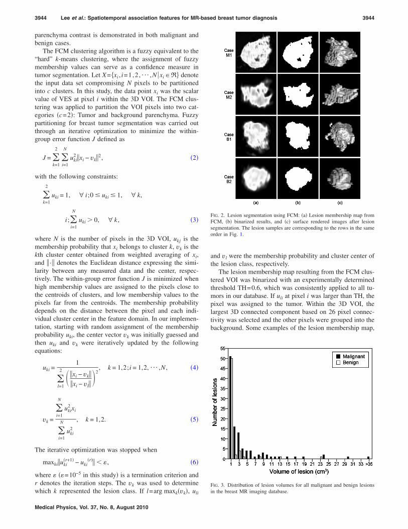
The lesion membership map resulting from the FCM clus-tered VOI was binarized with an experimentally determinedthreshold TH=0.6, which was consistently applied to all tu-mors in our database. If uli at pixel i was larger than TH, thepixel was assigned to the tumor. Within the 3D VOI, thelargest 3D connected component based on 26 pixel connec-tivity was selected and the other pixels were grouped into thebackground. Some examples of the lesion membership map,
FIG. 2. Lesion segmentation using FCM: �a� Lesion membership map fromFCM, �b� binarized results, and �c� surface rendered images after lesionsegmentation. The lesion samples are corresponding to the rows in the sameorder in Fig. 1.
FIG. 3. Distribution of lesion volumes for all malignant and benign lesions
in the breast MR imaging database.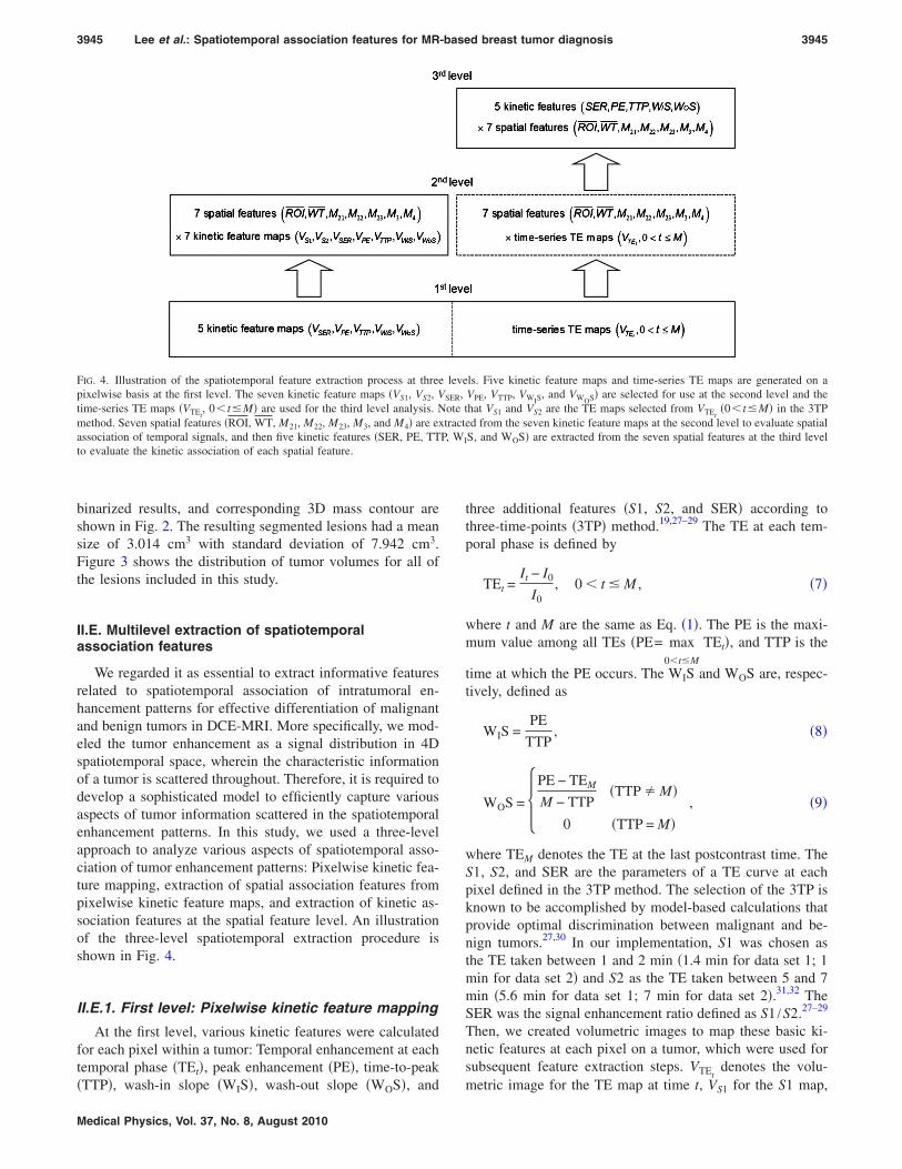
3945 Lee et al.: Spatiotemporal association features for MR-based breast tumor diagnosis 3945
binarized results, and corresponding 3D mass contour areshown in Fig. 2. The resulting segmented lesions had a meansize of 3.014 cm3 with standard deviation of 7.942 cm3.Figure 3 shows the distribution of tumor volumes for all ofthe lesions included in this study.
II.E. Multilevel extraction of spatiotemporalassociation features
We regarded it as essential to extract informative featuresrelated to spatiotemporal association of intratumoral en-hancement patterns for effective differentiation of malignantand benign tumors in DCE-MRI. More specifically, we mod-eled the tumor enhancement as a signal distribution in 4Dspatiotemporal space, wherein the characteristic informationof a tumor is scattered throughout. Therefore, it is required todevelop a sophisticated model to efficiently capture variousaspects of tumor information scattered in the spatiotemporalenhancement patterns. In this study, we used a three-levelapproach to analyze various aspects of spatiotemporal asso-ciation of tumor enhancement patterns: Pixelwise kinetic fea-ture mapping, extraction of spatial association features frompixelwise kinetic feature maps, and extraction of kinetic as-sociation features at the spatial feature level. An illustrationof the three-level spatiotemporal extraction procedure isshown in Fig. 4.
II.E.1. First level: Pixelwise kinetic feature mapping
At the first level, various kinetic features were calculatedfor each pixel within a tumor: Temporal enhancement at eachtemporal phase �TEt�, peak enhancement �PE�, time-to-peak
FIG. 4. Illustration of the spatiotemporal feature extraction process at threepixelwise basis at the first level. The seven kinetic feature maps �VS1, VS2, Vtime-series TE maps �VTEt
, 0� t�M� are used for the third level analysis. Nmethod. Seven spatial features �ROI, WT, M21, M22, M23, M3, and M4� are exassociation of temporal signals, and then five kinetic features �SER, PE, TTto evaluate the kinetic association of each spatial feature.
�TTP�, wash-in slope �WIS�, wash-out slope �WOS�, and
Medical Physics, Vol. 37, No. 8, August 2010
three additional features �S1, S2, and SER� according tothree-time-points �3TP� method.19,27–29 The TE at each tem-poral phase is defined by
TEt =It − I0
I0, 0 � t � M , �7�
where t and M are the same as Eq. �1�. The PE is the maxi-mum value among all TEs �PE= max
0�t�M
TEt�, and TTP is the
time at which the PE occurs. The WIS and WOS are, respec-tively, defined as
WIS =PE
TTP, �8�
WOS = �PE − TEM
M − TTP�TTP � M�
0 �TTP = M� , �9�
where TEM denotes the TE at the last postcontrast time. TheS1, S2, and SER are the parameters of a TE curve at eachpixel defined in the 3TP method. The selection of the 3TP isknown to be accomplished by model-based calculations thatprovide optimal discrimination between malignant and be-nign tumors.27,30 In our implementation, S1 was chosen asthe TE taken between 1 and 2 min �1.4 min for data set 1; 1min for data set 2� and S2 as the TE taken between 5 and 7min �5.6 min for data set 1; 7 min for data set 2�.31,32 TheSER was the signal enhancement ratio defined as S1 /S2.27–29
Then, we created volumetric images to map these basic ki-netic features at each pixel on a tumor, which were used forsubsequent feature extraction steps. VTEt
denotes the volu-
ls. Five kinetic feature maps and time-series TE maps are generated on aVPE, VTTP, VWIS
, and VWOS� are selected for use at the second level and thehat VS1 and VS2 are the TE maps selected from VTEt
�0� t�M� in the 3TPed from the seven kinetic feature maps at the second level to evaluate spatialS, and WOS� are extracted from the seven spatial features at the third level
leve
SER,ote ttract
P, WI
metric image for the TE map at time t, VS1 for the S1 map,
3946 Lee et al.: Spatiotemporal association features for MR-based breast tumor diagnosis 3946
VS2 for the S2 map, VSER for the SER map, VPE for the PEmap, VTTP for the TTP map, VWIS
for the WIS map, and VWOS
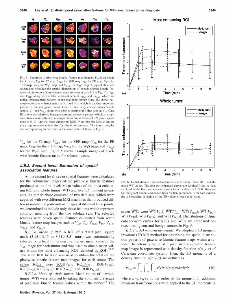
for the WOS map. Figure 5 shows example images of pixel-wise kinetic feature maps for selected cases.
II.E.2. Second level: Extraction of spatialassociation features
At the second level, seven spatial features were calculatedfor the volumetric images of the pixelwise kinetic featuresproduced at the first level: Mean values of the most enhanc-ing ROI and whole tumor �WT� and five 3D moment invari-ants. As our database consisted of two data sets, which wereacquired with two different MRI machines that produced dif-ferent number of postcontrast images at different time points,we determined to include only those features which representcommon meaning from the two subdata sets. The selectedfeatures were seven spatial features calculated from sevenkinetic feature map images such as VS1, VS2, VSER, VPE, VTTP,VWIS
, and VWOS.II.E.2.a. Mean of ROI. A ROI of a 9�9 pixel square
mask �3.15�3.15 to 3.51�3.51 mm2� was automaticallyselected on a location having the highest mean value in theVS1 image for each tumor and was used to obtain mean val-ues within the most enhancing ROI �denoted as ROI�.33,34
The same ROI location was used to obtain the ROI on thepixelwise kinetic feature map images for each tumor. Theseven ROIs were ROI�VS1�, ROI�VS2�, ROI�VSER�,ROI�VPE�, ROI�VTTP�, ROI�VWIS
�, and ROI�VWOS�.II.E.2.b. Mean of whole tumor. Mean values of a whole
tumor �WT� were obtained by taking the volumetric average35
FIG. 5. Examples of pixelwise kinetic feature map images. VS1 is an imagefor S1 map, VS2 for S2 map, VSER for SER map, VPE for PE map, VTTP forTTP map, VWIS
for WIS map, and VWOS for WOS map. A typical slice wasselected to visualize the spatial distribution of pseudocolored kinetic fea-tures within tumors. Rim enhancements are seen in case M1 at VS1, VS2, VPE,and VTTP, along with a later wash-out seen at VSER and VWOS, which aretypical enhancement patterns of the malignant tumor. Case M2 shows het-erogeneous area enhancements at VS1 and VS2, which is another importantpattern of the malignant tumor. Case B1 has early central enhancementsseen at VS1 and VWIS
along with delayed peripheral filling seen at VS2. CaseB2 shows the relatively homogeneous enhancement pattern, which is a typi-cal enhancement pattern of a benign tumor. Small boxes �9�9 pixel squaremasks� in VS1 are the most enhancing ROIs. Note that the kinetic featuremaps represent the scaled size for visual convenience. The tumor samplesare corresponding to the rows in the same order of those in Fig. 2.
of pixelwise kinetic feature values within the tumor. The
Medical Physics, Vol. 37, No. 8, August 2010
seven WTs were WT�VS1�, WT�VS2�, WT�VSER�, WT�VPE�,WT�VTTP�, WT�VWIS
�, and WT�VWOS�. Distributions of timeenhancement curves for ROIs and WTs are compared be-tween malignant and benign tumors in Fig. 6.
II.E.2.c. 3D moment invariants. We adopted a 3D momentinvariant �3D MI� method for describing the spatial distribu-tion patterns of pixelwise kinetic feature maps within a tu-mor. The intensity value of a pixel in a volumetric featuremap image is represented as a density function ��x ,y ,z� ofCartesian coordinate system. Then, the 3D moments of adensity function ��x ,y ,z� are defined as
mpqr = �−�
� �−�
� �−�
�
xpyqzr��x,y,z�dxdydz , �10�
where n= p+q+r is the order of the moment. In addition,
FIG. 6. Distribution of time enhancement curves for �a� mean ROI and �b�mean WT values. The four postenhanced curves are resulted from the dataset 1, while the five postenhanced curves form the data set 2. Solid lines arefor malignant tumors and dotted lines for benign tumors. Error bars indicatethe �1 standard deviation of the TE values in each time point.
invariant transformations were applied to the 3D moments in
3947 Lee et al.: Spatiotemporal association features for MR-based breast tumor diagnosis 3947
order to capture unique spatial features independent to shift,rotation, or scale caused by variations in patient postures orparticular coordinate system used in imaging system. Thetranslational invariance was obtained by using central mo-ments defined as
pqr = �−�
� �−�
� �−�
�
�x − x�p�y − y�q�z − z�r��x,y,z�dxdydz ,
�11�
where x, y, and z are the centroid coordinates of the densityfunction ��x ,y ,z�, calculated as
x =m100
m000, y =
m010
m000, z =
m001
m000. �12�
For scale invariance, the central moments were additionallynormalized as follows:
pqr =pqr
000��p+q+r�/3�+1 . �13�
In order to obtain rotational invariance, the normalized cen-tral moments were transformed into linear combinations ofmoments of the same order. A total of five 3D MIs were usedin this study, three of which were based on the second ordermoments derived by Sadjadi and Hall,36 and the remaininghigher order MIs were derived based on moment tensor con-traction according to Ng et al.37 With the normalized 3Dcentral moments, the second order 3D MIs can be written as
M21 = 200 + 020 + 002, �14�
M22 = 200020 + 200002 + 020002 − 1012 − 110
2 − 0112 ,
�15�
M23 = 200020002 − 0021102 + 2110101011 − 020101
2
− 2000112 . �16�
The derived higher order 3D MIs are as follows:
M3 = 3002 + 030
2 + 0032 + 3210
2 + 32012 + 3120
2 + 61112
+ 31022 + 3021
2 + 30122 , �17�
M4 = 4002 + 040
2 + 0042 + 4310
2 + 43012 + 6220
2 + 122112
+ 62022 + 4130
2 + 121212 + 12112
2 + 41032 + 4031
2
+ 60222 + 4013
2 . �18�
These 3D MIs were calculated for the seven pixelwise ki-netic feature map images, generating a 5�7 array of the 3DMIs. Thus, this array of the 3D MIs contain comprehensiveinformation on various aspects of volumetric spatial distribu-tion pattern for each pixelwise kinetic feature. The 5�7 3DMI values are denoted as M21�VS1� to M4�VS1�, M21�VS2� toM4�VS2�, M21�VSER� to M4�VSER�, M21�VPE� to M4�VPE�,M21�VTTP� to M4�VTTP�, M21�VWIS
� to M4�VWIS�, and
M21�VWOS� to M4�VWOS�.
Medical Physics, Vol. 37, No. 8, August 2010
II.E.3. Third level: Extraction of kinetic associationfeatures
At the third level, the five kinetic features SER, PE, TTP,WIS, and WOS were additionally measured for the time-series of seven spatial features to extract additional informa-tion on kinetic association of spatial features within a tumor.At this stage, the seven spatial features were first calculatedfor the time-series pixelwise TE maps �VTEt
, 0� t�M�, cre-ating additional time-series sets of the spatial features thatwere not included into the second level feature set. As thenumber of TEs in data sets 1 and 2 were 4 and 5, respec-tively, 7�4 spatial feature components were created for dataset 1 and 7�5 spatial feature components were created fordata set 2. And then, for each time-series set of the sevenspatial features, the above five kinetic features were calcu-lated to evaluate the kinetic association of spatial featureswithin a tumor. For example, PE�ROI� was obtained as themaximum value among the ROI�VTEt
� �0� t�M� andTTP�ROI� was the time at which the PE�ROI� occurred. Therationale behind this application is based on the assumptionthat the kinetic properties evaluated from time-series of spa-tial features may provide additional information that is notavailable in spatial features calculated for the pixelwise ki-netic feature maps. Thus, a total of 7�5 kinetic feature com-ponents were created at the third level: SER�ROI�,SER�WT�, SER�M21� to SER�M4�, PE�ROI�, PE�WT�,PE�M21� to PE�M4�, TTP�ROI�, TTP�WT�, TTP�M21� toTTP�M4�, WIS�ROI�, WIS�WT�, WIS�M21� to WIS�M4�,WOS�ROI�, WOS�WT�, and WOS�M21� to WOS�M4�.
II.F. Predictable values of single features
Our three-level feature extraction procedures produced atotal of 7�12 components of spatiotemporal features: 7�7 spatial feature components at the second level and 7�5 kinetic feature components at the third level. While mostof these features are spatiotemporal association features thatreflect either spatial associations of pixelwise kinetic patternsor kinetic associations of serial spatial properties of tumorenhancements, a subset of them includes relatively simplefeatures that represent only spatial or kinetic aspects of tu-mor enhancements as most of conventional morphologic orkinetic features do. We selected a set of simple featuresamong our feature array, and used them as references in per-formance comparison with the spatiotemporal associationfeatures. In the second level features, the seven spatial fea-tures calculated on VS1 were set as simple spatial features, asthey represent the spatial properties of only the initial TEimage, which are equivalent to conventional form of mor-phological features. In the third level features, the five ki-netic features calculated on only ROI means were set assimple kinetic features, which are the frequently used con-ventional kinetic features.
The predictable values of each single feature were evalu-ated by measuring the area under the receiver operating char-acteristic curve �Az� using a simple thresholding techniquewith varying threshold values for the features obtained from
all 171 tumor cases. A statistical significance testing was also
3948 Lee et al.: Spatiotemporal association features for MR-based breast tumor diagnosis 3948
performed using a z-test to assess the performance improve-ment of the spatiotemporal association features over thesimple features.38 In this statistical significance testing, thepredictable values were compared among the same kind offeatures in a pairwise manner between a simple feature andeach of its corresponding association features. For example,M21�VS1� �simple feature� was compared to each of M21�VS2�to M21�VWOS� �association features�. The calculation of Az
values and statistical testing for evaluating their differencewere performed using MEDCALC statistical software �MED-
CALC software version 11.2.1.0, Mariakerke, Belgium�.
II.G. Feature selection
Feature selection was performed using a support vectormachine-recursive feature elimination �SVM-RFE� algo-rithm. The SVM-RFE was originally proposed to performgene selection for cancer classification39 and was proved tobe effective in the selection of an optimal subset of featuresfrom a large number of features.40 This algorithm determinesthe ranking of each feature based on a sequential backwardelimination manner that removes one feature at a time, andsearches for a nonlinear separating margin to obtain the op-timal hyperplane in the feature space.41
In a two-class classification problem, m training samples�xk ,ykk=1
m �Rn� �−1,1 consist of the input feature sets xk
and the known class labels yk. The SVM algorithm first mapsthe inputs xk into a high dimensional feature space via anonlinear mapping function �� · � then computes a decisionfunction of the form42
g�x� = wT��x� + b �19�
by maximizing the distance between the set of points ��xk�to the hyperplane parametrized by the weighted vector w andthe bias term b, while being consistent on the training set.The class label of x is obtained by considering the sign ofg�x�. The learning task in the SVM can be formalized as thefollowing constrained optimization problem:
minw,b,�
1
2wTw + C
k=1
m
�k,
subject to ykg�xk� 1 − �k, �k 0, ∀ k , �20�
where C is the regularization parameter, which is a tradeoffbetween the training accuracy and the prediction term. WhenC is large, the error term is emphasized. A small C meansthat the large classification margin is encouraged. � is a mea-sure of the number of misclassifications and known as theslack variable. The solution of this problem is obtained usingthe Lagrangian theory and one can prove that vector w is ofthe form
w = k=1
Ns
�kyk��xk� , �21�
where �k are the Lagrange multipliers and �k�0. Ns is thenumber of training samples xk which correspond to �k�0.
Vectors xk for which �k�0 are called support vectors and theMedical Physics, Vol. 37, No. 8, August 2010
closest ones to the separating hyperplane. The �k is the so-lution of the following quadratic programming �QP�problem:42
max�
W��� = k=1
m
�k −1
2k,l
m
�k�lykyl�K�xk,xl� +1
C�k,l� ,
subject to k=1
m
yk�k = 0 and ∀ k, �k 0, �22�
where �k,l is the Kronecker symbol and K�xk ,xl�=��xk�T��xl� is the Gram matrix of the training data. Thethreshold b is chosen to maximize the margin and is given by
b = −maxyk=−1�wTxk� + minyk=+1�wTxk�
2. �23�
The decision function given by the SVM becomes
g�x� = wT��x� + b = k=1
Ns
�kykK�x,xk� + b . �24�
We apply the zero-order method for identifying the vari-able that produces the smallest value of the ranking criterionwhen removed and use the weight magnitude �w�2 as rankingcriterion, defined as
�w�i��2 = j=1
Ns
k=1
Ns
�k�i�� j
�i�ykyjK�i��xk,xj� , �25�
where K�i� is the Gram matrix of the training data when thevariable i is removed and ��i� is the corresponding solutionof the SVM classifier. The rationale of the ranking criterionis that the inputs which are weighted by the largest valuehave the most influence on the classification decision. Con-sequently, if the classifier performs well, those inputs withthe largest weights correspond to the most informative fea-tures. In the implementation of SVM-RFE, we used a radialbasis function �RBF� kernel of which K�xi ,xj�=exp�−�xi
−xj�2 /�2� with �=1 for the nonlinear problem, and set thehyperparameter C to be sufficiently high �C=103� in order tokeep training error low.
II.H. Tumor differentiation
By using the rank data, we identified several optimal fea-ture sets for use in the final tumor classification. Identifica-tion of an optimal feature set was performed by applying aleast-squares support vector machine �LS-SVM� classifier toa sequential forward inclusion procedure.43 The LS-SVM is amodified version of the standard SVM, and is known to beadvantageous in handling a large dimensional data and find-ing an optimal separation based on the limited amount ofavailable training data, without dimensionality reduction.44
In principle, LS-SVM simplifies the formulation by re-placing the inequality constraint in SVM with an equalityconstraint. This approach significantly reduces the cost in
complexity and computation time, solving a set of linear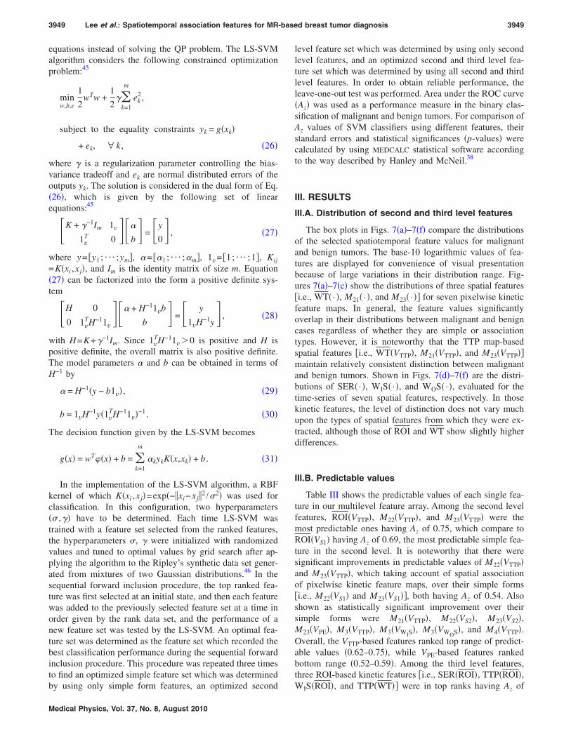
3949 Lee et al.: Spatiotemporal association features for MR-based breast tumor diagnosis 3949
equations instead of solving the QP problem. The LS-SVMalgorithm considers the following constrained optimizationproblem:45
minw,b,e
1
2wTw +
1
2�
k=1
m
ek2,
subject to the equality constraints yk = g�xk�
+ ek, ∀ k , �26�
where � is a regularization parameter controlling the bias-variance tradeoff and ek are normal distributed errors of theoutputs yk. The solution is considered in the dual form of Eq.�26�, which is given by the following set of linearequations:45
�K + �−1Im 1v
1vT 0
���
b� = �y
0� , �27�
where y= �y1 ; ¯ ;ym�, �= ��1 ; ¯ ;�m�, 1v= �1; ¯ ;1�, Kij
=K�xi ,xj�, and Im is the identity matrix of size m. Equation�27� can be factorized into the form a positive definite sys-tem
�H 0
0 1vTH−11v
��� + H−11vb
b� = � y
1vH−1y� , �28�
with H=K+�−1Im. Since 1vTH−11v�0 is positive and H is
positive definite, the overall matrix is also positive definite.The model parameters � and b can be obtained in terms ofH−1 by
� = H−1�y − b1v� , �29�
b = 1vH−1y�1vTH−11v�−1. �30�
The decision function given by the LS-SVM becomes
g�x� = wT��x� + b = k=1
m
�kykK�x,xk� + b . �31�
In the implementation of the LS-SVM algorithm, a RBFkernel of which K�xi ,xj�=exp�−�xi−xj�2 /�2� was used forclassification. In this configuration, two hyperparameters�� ,�� have to be determined. Each time LS-SVM wastrained with a feature set selected from the ranked features,the hyperparameters �, � were initialized with randomizedvalues and tuned to optimal values by grid search after ap-plying the algorithm to the Ripley’s synthetic data set gener-ated from mixtures of two Gaussian distributions.46 In thesequential forward inclusion procedure, the top ranked fea-ture was first selected at an initial state, and then each featurewas added to the previously selected feature set at a time inorder given by the rank data set, and the performance of anew feature set was tested by the LS-SVM. An optimal fea-ture set was determined as the feature set which recorded thebest classification performance during the sequential forwardinclusion procedure. This procedure was repeated three timesto find an optimized simple feature set which was determined
by using only simple form features, an optimized secondMedical Physics, Vol. 37, No. 8, August 2010
level feature set which was determined by using only secondlevel features, and an optimized second and third level fea-ture set which was determined by using all second and thirdlevel features. In order to obtain reliable performance, theleave-one-out test was performed. Area under the ROC curve�Az� was used as a performance measure in the binary clas-sification of malignant and benign tumors. For comparison ofAz values of SVM classifiers using different features, theirstandard errors and statistical significances �p-values� werecalculated by using MEDCALC statistical software accordingto the way described by Hanley and McNeil.38
III. RESULTS
III.A. Distribution of second and third level features
The box plots in Figs. 7�a�–7�f� compare the distributionsof the selected spatiotemporal feature values for malignantand benign tumors. The base-10 logarithmic values of fea-tures are displayed for convenience of visual presentationbecause of large variations in their distribution range. Fig-ures 7�a�–7�c� show the distributions of three spatial features�i.e., WT� · �, M21� · �, and M23� · �� for seven pixelwise kineticfeature maps. In general, the feature values significantlyoverlap in their distributions between malignant and benigncases regardless of whether they are simple or associationtypes. However, it is noteworthy that the TTP map-basedspatial features �i.e., WT�VTTP�, M21�VTTP�, and M23�VTTP��maintain relatively consistent distinction between malignantand benign tumors. Shown in Figs. 7�d�–7�f� are the distri-butions of SER� · �, WIS� · �, and WOS� · �, evaluated for thetime-series of seven spatial features, respectively. In thosekinetic features, the level of distinction does not vary muchupon the types of spatial features from which they were ex-tracted, although those of ROI and WT show slightly higherdifferences.
III.B. Predictable values
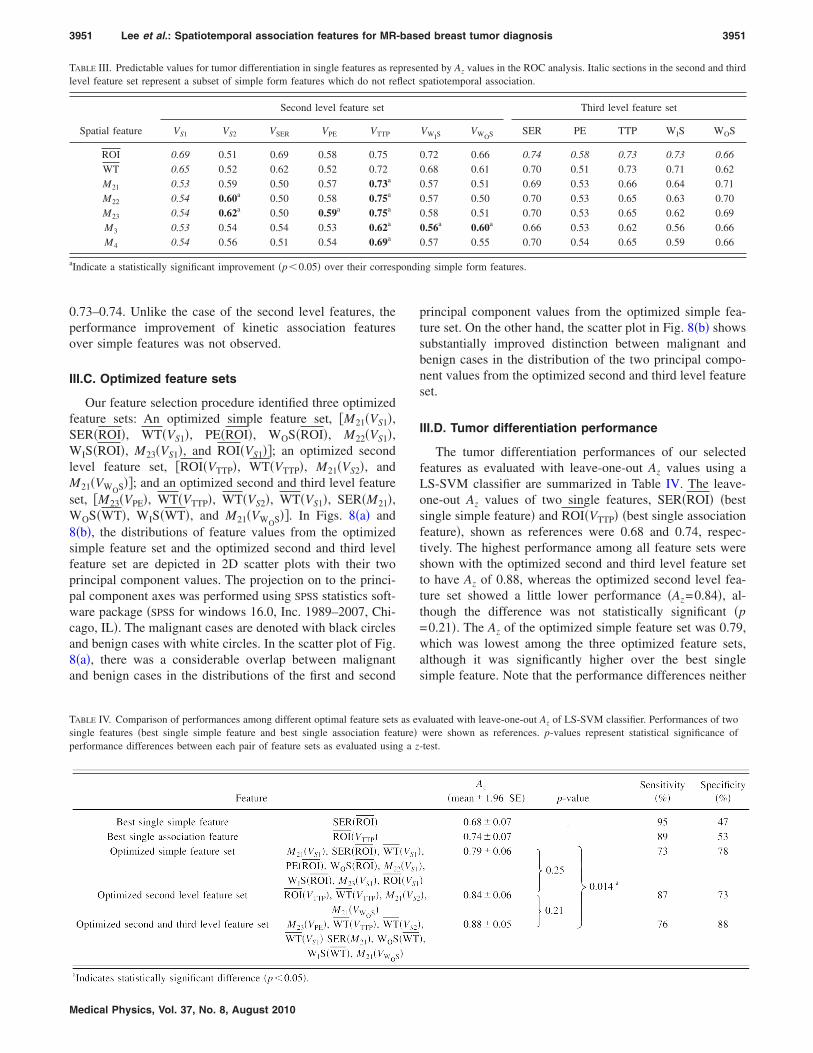
Table III shows the predictable values of each single fea-ture in our multilevel feature array. Among the second levelfeatures, ROI�VTTP�, M22�VTTP�, and M23�VTTP� were themost predictable ones having Az of 0.75, which compare toROI�VS1� having Az of 0.69, the most predictable simple fea-ture in the second level. It is noteworthy that there weresignificant improvements in predictable values of M22�VTTP�and M23�VTTP�, which taking account of spatial associationof pixelwise kinetic feature maps, over their simple forms�i.e., M22�VS1� and M23�VS1��, both having Az of 0.54. Alsoshown as statistically significant improvement over theirsimple forms were M21�VTTP�, M22�VS2�, M23�VS2�,M23�VPE�, M3�VTTP�, M3�VWIS
�, M3�VWOS�, and M4�VTTP�.Overall, the VTTP-based features ranked top range of predict-able values �0.62–0.75�, while VPE-based features rankedbottom range �0.52–0.59�. Among the third level features,three ROI-based kinetic features �i.e., SER�ROI�, TTP�ROI�,
WIS�ROI�, and TTP�WT�� were in top ranks having Az of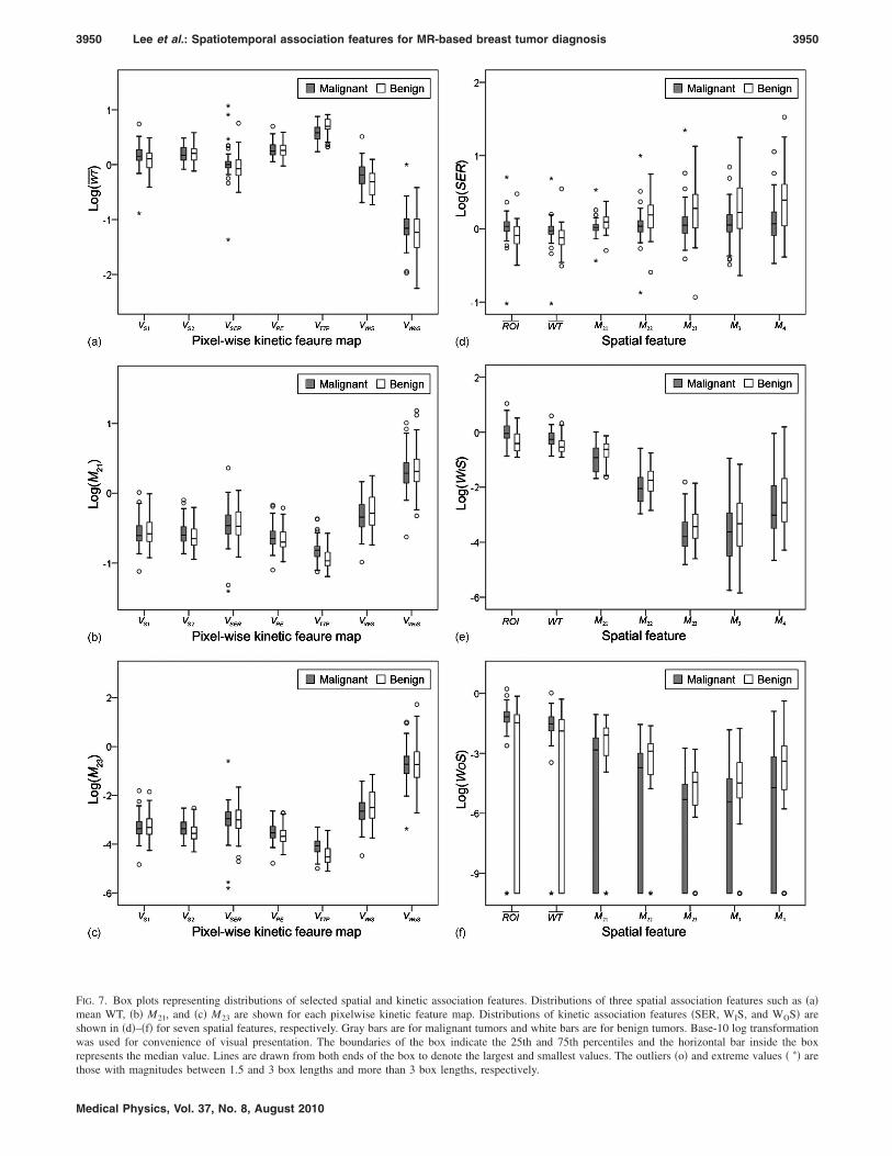
3950 Lee et al.: Spatiotemporal association features for MR-based breast tumor diagnosis 3950
FIG. 7. Box plots representing distributions of selected spatial and kinetic association features. Distributions of three spatial association features such as �a�mean WT, �b� M21, and �c� M23 are shown for each pixelwise kinetic feature map. Distributions of kinetic association features �SER, WIS, and WOS� areshown in �d�–�f� for seven spatial features, respectively. Gray bars are for malignant tumors and white bars are for benign tumors. Base-10 log transformationwas used for convenience of visual presentation. The boundaries of the box indicate the 25th and 75th percentiles and the horizontal bar inside the boxrepresents the median value. Lines are drawn from both ends of the box to denote the largest and smallest values. The outliers �o� and extreme values � �� are
those with magnitudes between 1.5 and 3 box lengths and more than 3 box lengths, respectively.Medical Physics, Vol. 37, No. 8, August 2010
ondi
3951 Lee et al.: Spatiotemporal association features for MR-based breast tumor diagnosis 3951
0.73–0.74. Unlike the case of the second level features, theperformance improvement of kinetic association featuresover simple features was not observed.
III.C. Optimized feature sets
Our feature selection procedure identified three optimizedfeature sets: An optimized simple feature set, �M21�VS1�,SER�ROI�, WT�VS1�, PE�ROI�, WOS�ROI�, M22�VS1�,WIS�ROI�, M23�VS1�, and ROI�VS1��; an optimized secondlevel feature set, �ROI�VTTP�, WT�VTTP�, M21�VS2�, andM21�VWOS��; and an optimized second and third level featureset, �M23�VPE�, WT�VTTP�, WT�VS2�, WT�VS1�, SER�M21�,WOS�WT�, WIS�WT�, and M21�VWOS��. In Figs. 8�a� and8�b�, the distributions of feature values from the optimizedsimple feature set and the optimized second and third levelfeature set are depicted in 2D scatter plots with their twoprincipal component values. The projection on to the princi-pal component axes was performed using SPSS statistics soft-ware package �SPSS for windows 16.0, Inc. 1989–2007, Chi-cago, IL�. The malignant cases are denoted with black circlesand benign cases with white circles. In the scatter plot of Fig.8�a�, there was a considerable overlap between malignantand benign cases in the distributions of the first and second
TABLE III. Predictable values for tumor differentiation in single features as relevel feature set represent a subset of simple form features which do not re
Spatial feature
Second level feature set
VS1 VS2 VSER VPE VTTP
ROI 0.69 0.51 0.69 0.58 0.75WT 0.65 0.52 0.62 0.52 0.72M21 0.53 0.59 0.50 0.57 0.73a
M22 0.54 0.60a 0.50 0.58 0.75a
M23 0.54 0.62a 0.50 0.59a 0.75a
M3 0.53 0.54 0.54 0.53 0.62a
M4 0.54 0.56 0.51 0.54 0.69a
aIndicate a statistically significant improvement �p�0.05� over their corresp
TABLE IV. Comparison of performances among different optimal feature setssingle features �best single simple feature and best single association feaperformance differences between each pair of feature sets as evaluated usin
Medical Physics, Vol. 37, No. 8, August 2010
principal component values from the optimized simple fea-ture set. On the other hand, the scatter plot in Fig. 8�b� showssubstantially improved distinction between malignant andbenign cases in the distribution of the two principal compo-nent values from the optimized second and third level featureset.
III.D. Tumor differentiation performance
The tumor differentiation performances of our selectedfeatures as evaluated with leave-one-out Az values using aLS-SVM classifier are summarized in Table IV. The leave-one-out Az values of two single features, SER�ROI� �bestsingle simple feature� and ROI�VTTP� �best single associationfeature�, shown as references were 0.68 and 0.74, respec-tively. The highest performance among all feature sets wereshown with the optimized second and third level feature setto have Az of 0.88, whereas the optimized second level fea-ture set showed a little lower performance �Az=0.84�, al-though the difference was not statistically significant �p=0.21�. The Az of the optimized simple feature set was 0.79,which was lowest among the three optimized feature sets,although it was significantly higher over the best singlesimple feature. Note that the performance differences neither
nted by Az values in the ROC analysis. Italic sections in the second and thirdpatiotemporal association.
Third level feature set
VWISVWOS SER PE TTP WIS WOS
0.72 0.66 0.74 0.58 0.73 0.73 0.660.68 0.61 0.70 0.51 0.73 0.71 0.620.57 0.51 0.69 0.53 0.66 0.64 0.710.57 0.50 0.70 0.53 0.65 0.63 0.700.58 0.51 0.70 0.53 0.65 0.62 0.690.56a 0.60a 0.66 0.53 0.62 0.56 0.660.57 0.55 0.70 0.54 0.65 0.59 0.66
ng simple form features.
aluated with leave-one-out Az of LS-SVM classifier. Performances of twowere shown as references. p-values represent statistical significance of-test.
preseflect s
as evture�g a z

3952 Lee et al.: Spatiotemporal association features for MR-based breast tumor diagnosis 3952
between the optimized simple feature set and the optimizedsecond level feature set nor between the optimized secondlevel feature set and the optimized second and third level
FIG. 8. 2D scatter plots compare the distributions of first and second prin-cipal component values for the tumor cases taken from �a� the optimizedsimple feature set and �b� optimized second and third level feature set.White circles denote benign cases and black circles denote malignant cases.Note that there was a significant overlap between malignant and benigntumors in the distribution of two principal component values in �a�, whereasa substantially improved distinction is noticed between malignant and be-nign tumors in the distribution of two principal component values in �b�.
feature set were statistically significant �p=0.25 and 0.21�,
Medical Physics, Vol. 37, No. 8, August 2010
whereas improvement of the optimized second and thirdlevel feature set over the optimized simple feature set wasstatistically significant �p=0.014�.
The ROC curves of the two best single features and threeoptimized feature sets were depicted in Fig. 9. The smoothROC curves were plotted using JROCFIT.47 The optimizedsecond and third level feature set shows the highest sensitiv-ity at most specificity levels over the other features, followedby the optimized second level feature set, optimized simplefeature set, best single association feature �ROI�VTTP��, andbest single simple feature �SER�ROI��.
Figure 10 shows the changes of classification accuracy�Az� of LS-SVM according to the number of features in-cluded in order, as ranked by SVM-RFE from the combinedsecond and third level features. The accuracy increasesabruptly up to its highest peak at the number 8, and thenshows a decreasing tendency along with some fluctuationslater on. This suggests that the redundant features have to beidentified and eliminated in order to yield a best classifica-tion performance and that how to determine the ranks ofeach feature should be chosen carefully.
IV. DISCUSSION
IV.A. Postulate of this study
Breast DCE-MRI represents the challenges faced in radio-logical interpretation of multidimensional imaging data to-day. Dynamic 3D images are produced during the timecourse of contrast enhancement, which contain rich informa-tion involving functional and anatomical aspects of breasttissues. However, capturing and interpreting of complex spa-tiotemporal signal patterns in such dynamic 3D images ineveryday practices surpass human ability. This mismatch be-tween the efficiencies of image production and interpretationoften causes intraobserver and interobserver variability in di-agnostic performance and makes a bottleneck in diagnosticworkflow as well in breast DCE-MRI.48 Therefore, the mo-tivation of this study was to develop a CAD scheme that caneffectively characterize such spatiotemporal signal patternsof tumor enhancement in multidimensional image data set inDCE-MRI.
In this study, we postulated that analyzing spatiotemporalassociation would provide additional information on tumordifferentiation that was not attainable using conventional ap-proaches in which spatial or temporal features were extractedseparately. Based on this postulation, we presented a novelapproach to breast MRI CAD using a multilevel analysis ofspatiotemporal association features for tumor enhancementpatterns in DCE-MRI. Spatial association features �secondlevel features� for pixelwise kinetic patterns as well as ki-netic association features �third level features� for time-seriesof spatial features were extracted in the proposed multilevelfeature extraction procedure.
IV.B. Testing of postulate
In order to test our postulate, we first evaluated the per-
formance improvements of our spatiotemporal association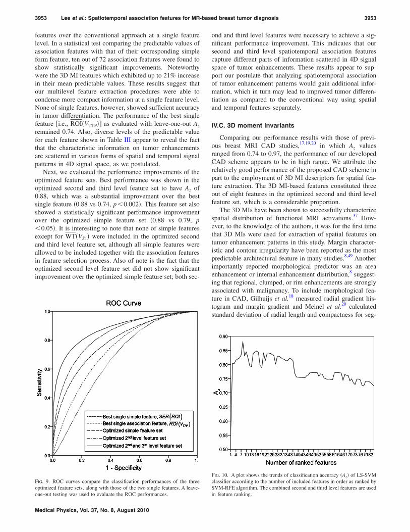
3953 Lee et al.: Spatiotemporal association features for MR-based breast tumor diagnosis 3953
features over the conventional approach at a single featurelevel. In a statistical test comparing the predictable values ofassociation features with that of their corresponding simpleform feature, ten out of 72 association features were found toshow statistically significant improvements. Noteworthywere the 3D MI features which exhibited up to 21% increasein their mean predictable values. These results suggest thatour multilevel feature extraction procedures were able tocondense more compact information at a single feature level.None of single features, however, showed sufficient accuracyin tumor differentiation. The performance of the best singlefeature �i.e., ROI�VTTP�� as evaluated with leave-one-out Az
remained 0.74. Also, diverse levels of the predictable valuefor each feature shown in Table III appear to reveal the factthat the characteristic information on tumor enhancementsare scattered in various forms of spatial and temporal signalpatterns in 4D signal space, as we postulated.
Next, we evaluated the performance improvements of theoptimized feature sets. Best performance was shown in theoptimized second and third level feature set to have Az of0.88, which was a substantial improvement over the bestsingle feature �0.88 vs 0.74, p�0.002�. This feature set alsoshowed a statistically significant performance improvementover the optimized simple feature set �0.88 vs 0.79, p�0.05�. It is interesting to note that none of simple featuresexcept for WT�VS1� were included in the optimized secondand third level feature set, although all simple features wereallowed to be included together with the association featuresin feature selection process. Also of note is the fact that theoptimized second level feature set did not show significantimprovement over the optimized simple feature set; both sec-
FIG. 9. ROC curves compare the classification performances of the threeoptimized feature sets, along with those of the two single features. A leave-
one-out testing was used to evaluate the ROC performances.Medical Physics, Vol. 37, No. 8, August 2010
ond and third level features were necessary to achieve a sig-nificant performance improvement. This indicates that oursecond and third level spatiotemporal association featurescapture different parts of information scattered in 4D signalspace of tumor enhancements. These results appear to sup-port our postulate that analyzing spatiotemporal associationof tumor enhancement patterns would gain additional infor-mation, which in turn may lead to improved tumor differen-tiation as compared to the conventional way using spatialand temporal features separately.
IV.C. 3D moment invariants
Comparing our performance results with those of previ-ous breast MRI CAD studies,17,19,20 in which Az valuesranged from 0.74 to 0.97, the performance of our developedCAD scheme appears to be in high range. We attribute therelatively good performance of the proposed CAD scheme inpart to the employment of 3D MI descriptors for spatial fea-ture extraction. The 3D MI-based features constituted threeout of eight features in the optimized second and third levelfeature set, which is a considerable proportion.
The 3D MIs have been shown to successfully characterizespatial distribution of functional MRI activations.37 How-ever, to the knowledge of the authors, it was for the first timethat 3D MIs were used for extraction of spatial features ontumor enhancement patterns in this study. Margin character-istic and contour irregularity have been reported as the mostpredictable architectural feature in many studies.8,49 Anotherimportantly reported morphological predictor was an areaenhancement or internal enhancement distribution,8 suggest-ing that regional, clumped, or rim enhancements are stronglyassociated with malignancy. To include morphological fea-ture in CAD, Gilhuijs et al.18 measured radial gradient his-togram and margin gradient and Meinel et al.20 calculatedstandard deviation of radial length and compactness for seg-
FIG. 10. A plot shows the trends of classification accuracy �Az� of LS-SVMclassifier according to the number of included features in order as ranked bySVM-RFE algorithm. The combined second and third level features are used
in feature ranking.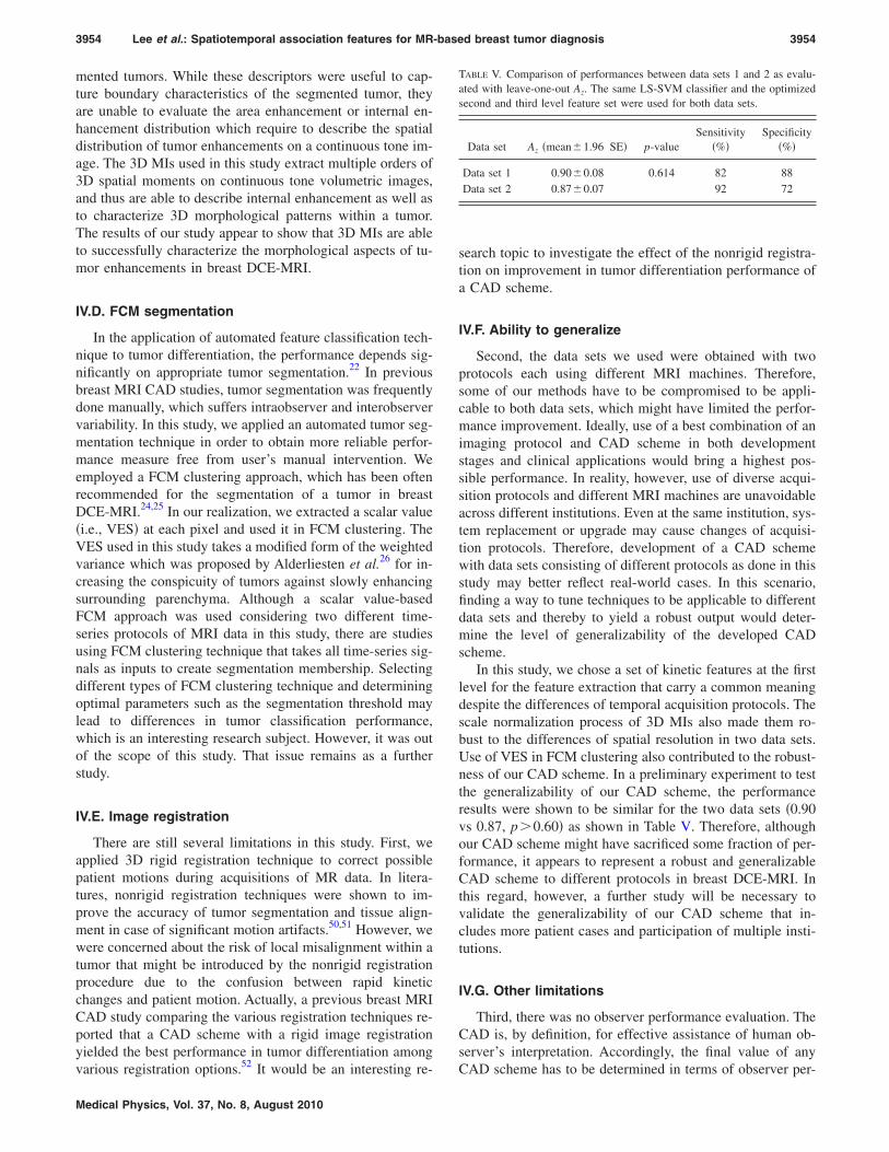
3954 Lee et al.: Spatiotemporal association features for MR-based breast tumor diagnosis 3954
mented tumors. While these descriptors were useful to cap-ture boundary characteristics of the segmented tumor, theyare unable to evaluate the area enhancement or internal en-hancement distribution which require to describe the spatialdistribution of tumor enhancements on a continuous tone im-age. The 3D MIs used in this study extract multiple orders of3D spatial moments on continuous tone volumetric images,and thus are able to describe internal enhancement as well asto characterize 3D morphological patterns within a tumor.The results of our study appear to show that 3D MIs are ableto successfully characterize the morphological aspects of tu-mor enhancements in breast DCE-MRI.
IV.D. FCM segmentation
In the application of automated feature classification tech-nique to tumor differentiation, the performance depends sig-nificantly on appropriate tumor segmentation.22 In previousbreast MRI CAD studies, tumor segmentation was frequentlydone manually, which suffers intraobserver and interobservervariability. In this study, we applied an automated tumor seg-mentation technique in order to obtain more reliable perfor-mance measure free from user’s manual intervention. Weemployed a FCM clustering approach, which has been oftenrecommended for the segmentation of a tumor in breastDCE-MRI.24,25 In our realization, we extracted a scalar value�i.e., VES� at each pixel and used it in FCM clustering. TheVES used in this study takes a modified form of the weightedvariance which was proposed by Alderliesten et al.26 for in-creasing the conspicuity of tumors against slowly enhancingsurrounding parenchyma. Although a scalar value-basedFCM approach was used considering two different time-series protocols of MRI data in this study, there are studiesusing FCM clustering technique that takes all time-series sig-nals as inputs to create segmentation membership. Selectingdifferent types of FCM clustering technique and determiningoptimal parameters such as the segmentation threshold maylead to differences in tumor classification performance,which is an interesting research subject. However, it was outof the scope of this study. That issue remains as a furtherstudy.
IV.E. Image registration
There are still several limitations in this study. First, weapplied 3D rigid registration technique to correct possiblepatient motions during acquisitions of MR data. In litera-tures, nonrigid registration techniques were shown to im-prove the accuracy of tumor segmentation and tissue align-ment in case of significant motion artifacts.50,51 However, wewere concerned about the risk of local misalignment within atumor that might be introduced by the nonrigid registrationprocedure due to the confusion between rapid kineticchanges and patient motion. Actually, a previous breast MRICAD study comparing the various registration techniques re-ported that a CAD scheme with a rigid image registrationyielded the best performance in tumor differentiation among
52
various registration options. It would be an interesting re-Medical Physics, Vol. 37, No. 8, August 2010
search topic to investigate the effect of the nonrigid registra-tion on improvement in tumor differentiation performance ofa CAD scheme.
IV.F. Ability to generalize
Second, the data sets we used were obtained with twoprotocols each using different MRI machines. Therefore,some of our methods have to be compromised to be appli-cable to both data sets, which might have limited the perfor-mance improvement. Ideally, use of a best combination of animaging protocol and CAD scheme in both developmentstages and clinical applications would bring a highest pos-sible performance. In reality, however, use of diverse acqui-sition protocols and different MRI machines are unavoidableacross different institutions. Even at the same institution, sys-tem replacement or upgrade may cause changes of acquisi-tion protocols. Therefore, development of a CAD schemewith data sets consisting of different protocols as done in thisstudy may better reflect real-world cases. In this scenario,finding a way to tune techniques to be applicable to differentdata sets and thereby to yield a robust output would deter-mine the level of generalizability of the developed CADscheme.
In this study, we chose a set of kinetic features at the firstlevel for the feature extraction that carry a common meaningdespite the differences of temporal acquisition protocols. Thescale normalization process of 3D MIs also made them ro-bust to the differences of spatial resolution in two data sets.Use of VES in FCM clustering also contributed to the robust-ness of our CAD scheme. In a preliminary experiment to testthe generalizability of our CAD scheme, the performanceresults were shown to be similar for the two data sets �0.90vs 0.87, p�0.60� as shown in Table V. Therefore, althoughour CAD scheme might have sacrificed some fraction of per-formance, it appears to represent a robust and generalizableCAD scheme to different protocols in breast DCE-MRI. Inthis regard, however, a further study will be necessary tovalidate the generalizability of our CAD scheme that in-cludes more patient cases and participation of multiple insti-tutions.
IV.G. Other limitations
Third, there was no observer performance evaluation. TheCAD is, by definition, for effective assistance of human ob-server’s interpretation. Accordingly, the final value of any
TABLE V. Comparison of performances between data sets 1 and 2 as evalu-ated with leave-one-out Az. The same LS-SVM classifier and the optimizedsecond and third level feature set were used for both data sets.
Data set Az �mean�1.96 SE� p-valueSensitivity
�%�Specificity
�%�
Data set 1 0.90�0.08 0.614 82 88Data set 2 0.87�0.07 92 72
CAD scheme has to be determined in terms of observer per-
3955 Lee et al.: Spatiotemporal association features for MR-based breast tumor diagnosis 3955
formance improvements. Therefore, an observer perfor-mance study is warranted to finally judge the value of ourdeveloped CAD scheme.
Finally, this study presented a multilevel feature extrac-tion approach to analyzing the spatiotemporal association oftumor enhancement patterns. Although our method showed apromising performance results, it was one of many possibleapproaches. An extended study to explore further potentialsof analyzing the spatiotemporal association of tumor en-hancement patterns will be a challenging and yet valuabletask to advance CAD techniques to find a more essential rolein future applications.
V. CONCLUSION
This work presented a novel approach to breast MRICAD based on multilevel analysis of spatiotemporal associa-tion features in tumor enhancement patterns. The spatiotem-poral association features derived by our multilevel analysisstrategy were shown to collect various aspects of character-istic tumor information effectively. By optimizing a featureset using these spatiotemporal association features and clas-sifying with LS-SVM, a high performance tumor classifica-tion was possible, achieving Az of 0.88.
Comparing with a feature set which does not reflect thespatiotemporal association, our multilevel feature analysisstrategy showed a statistically significant performance im-provement �p�0.05�. Our proposed CAD framework has apotential for improving diagnostic performance in breastDCE-MRI.
ACKNOWLEDGMENTS
This work was supported by the Seoul Research and Busi-ness Development Program �Grant No. 10888� and in part bya National Research Foundation of Korea �NRF� grantfunded by the Korean government �Grant No. 2009-0082064�.
a�Author to whom correspondence should be addressed. Electronic mail:[email protected]
b�Present address: Department of Radiology, Hanyang University Collegeof Medicine, Seoul 133-791, Korea.
1M. J. Stoutjesdijk, C. Boetes, G. J. Jager, L. Beex, P. Bult, J. H. Hendriks,R. J. Laheij, L. Massuger, L. E. van Die, T. Wobbes, and J. O. Barentsz,“Magnetic resonance imaging and mammography in women with a he-reditary risk of breast cancer,” J. Natl. Cancer Inst. 93, 1095–1102 �2001�.
2L. Liberman, “Breast cancer screening with MRI—What are the data forpatients at high risk?,” N. Engl. J. Med. 351, 497–500 �2004�.
3C. K. Kuhl, S. Schrading, C. C. Leutner, N. Morakkabati-Spitz, E. Ward-elmann, R. Fimmers, W. Kuhn, and H. H. Schild, “Mammography, breastultrasound, and magnetic resonance imaging for surveillance of women athigh familial risk for breast cancer,” J. Clin. Oncol. 23, 8469–8476�2005�.
4M. O. Leach, C. R. Boggis, A. K. Dixon, D. F. Easton, R. A. Eeles, D. G.Evans, F. J. Gilbert, I. Griebsch, R. J. Hoff, P. Kessar, S. R. Lakhani, S.M. Moss, A. Nerurkar, A. R. Padhani, L. J. Pointon, D. Thompson, R. M.Warren �MARIBS Study Group�, “Screening with magnetic resonanceimaging and mammography of a UK population at high risk of breastcancer: A prospective multicentre cohort study �MARIBS�,” Lancet 365,1769–1778 �2005�.
5F. Sardanelli, F. Podo, G. D’Agnolo, A. Verdecchia, M. Santaguilani, R.Musumeci, G. Trecate, S. Manoukian, S. Morassut, C. de Giacomi, M.
Federico, L. Cortesi, S. Corcione, S. Cirillo, V. Marra �High Breast Can-Medical Physics, Vol. 37, No. 8, August 2010
cer Risk Italian Trial�, A. Cilotti, C. Di Maggio, A. Fausto, L. Preda, C.Zuiani, A. Contegiacomo, A. Orlacchio, M. Calabrese, L. Bonomo, E. DiCesare, M. Tonutti, P. Panizza, and A. Del Maschio, and the , “Multi-center comparative multimodality surveillance of women at genetic-familial high risk for breast cancer �HIBCRIT�: Interim results,” Radiol-ogy 242, 698–715 �2007�.
6M. O. Leach, “Breast cancer screening in women at high risk using MRI,”NMR Biomed. 22, 17–27 �2009�.
7T. C. Williams, W. B. DeMartini, S. C. Partridge, S. Peacock, and C. D.Lehman, “Breast MR imaging: Computer-aided evaluation program fordiscriminating benign from malignant lesions,” Radiology 244, 94–103�2007�.
8M. D. Schnall, J. Blume, D. A. Bluemke, G. A. DeAngelis, N. DeBruhl,S. Harms, S. H. Heywang-Kobrunner, N. Hylton, C. K. Kuhl, E. D.Pisano, P. Causer, S. J. Schnitt, D. Thickman, C. B. Stelling, P. T. Weath-erall, C. Lehman, and C. A. Gatsonis, “Diagnostic architectural and dy-namic features at breast MR imaging: Multicenter study,” Radiology 238,42–53 �2006�.
9C. K. Kuhl, P. Mielcareck, S. Klaschik, C. Leutner, E. Wardelmann, J.Gieseke, and H. H. Schild, “Dynamic breast MR imaging: Are signalintensity time course data useful for differential diagnosis of enhancinglesions?,” Radiology 211, 101–110 �1999�.
10O. Ikeda, R. Nishimura, H. Miyayama, T. Yasunaga, Y. Ozaki, A. Tuji,and Y. Yamashita, “Evaluation of tumor angiogenesis using dynamic en-hanced magnetic resonance imaging: Comparison of plasma vascular en-dothelial growth factor, hemodynamic, and pharmacokinetic parameters,”Acta Radiol. 45, 446–452 �2004�.
11L. W. Nunes, M. D. Schnall, and S. G. Orel, “Update of breast MRimaging architectural interpretation model,” Radiology 219, 484–494�2001�.
12U. Wedegärtner, U. Bick, K. Wortler, E. Rummerny, and G. Bongartz,“Differentiation between benign and malignant findings on MR-mammography: Usefulness of morphological criteria,” Eur. Radiol. 11,1645–1650 �2001�.
13U. S. G. Orel, “Differentiating benign from malignant enhancing lesionsidentified at MR imaging of the breast: Are time signal-intensity curvesan accurate predictor?,” Radiology 211, 5–7 �1999�.
14S. Mussurakis, D. L. Buckley, and A. Horsman, “Dynamic MRI of inva-sive breast cancer: Assessment of three region-of-interest analysis meth-ods,” J. Comput. Assist. Tomogr. 21, 431–438 �1997�.
15ACR BI-RADS-MRI, 1st ed. �American College of Radiology, Reston, VA,2003�.
16R. E. Lucht, M. V. Knopp, and G. Brix, “Classification of signal-timecurves from dynamic MR mammography by neural networks,” Magn.Reson. Imaging 19, 51–57 �2001�.
17J. Levman, T. Leung, P. Causer, D. Plewes, and A. L. Martel, “Classifi-cation of dynamic contrast-enhanced magnetic resonance breast lesionsby support vector machines,” IEEE Trans. Med. Imaging 27, 688–696�2008�.
18K. G. Gilhuijs, M. L. Giger, and U. Bick, “Computerized analysis ofbreast lesions in three dimensions using dynamic magnetic-resonance im-aging,” Med. Phys. 25, 1647–1654 �1998�.
19W. Chen, M. L. Giger, L. Lan, and U. Bick, “Computerized interpretationof breast MRI: Investigation of enhancement-variance dynamics,” Med.Phys. 31, 1076–1082 �2004�.
20L. A. Meinel, A. H. Stolpen, K. S. Berbaum, L. L. Fajardo, and J. M.Reinhardt, “Breast MRI lesion classification: Improved performance ofhuman readers with a backpropagation neural network computer-aideddiagnosis �CAD� system,” J. Magn. Reson Imaging 25, 89–95 �2007�.
21Y. Zheng, S. Englander, M. D. Schnall, and D. Shen, “STEP: Spatial-temporal enhancement pattern, for MR-based breast tumor diagnosis,” inProceedings of the Fourth IEEE International Symposium on BiomedicalImaging: From to Nano to Macro, 2007 �IEEE, New York, 2007�, pp.520–523.
22Y. Zheng, S. Englander, S. Baloch, E. I. Zacharaki, Y. Fan, M. D. Schnall,and D. Shen, “STEP: Spatiotemporal enhancement pattern for MR-basedbreast tumor diagnosis,” Med. Phys. 36, 3192–3204 �2009�.
23W. M. Wells III, P. Viola, H. Atsumi, S. Nakajima, and R. Kikinis,“Multi-modal volume registration by maximization of mutual informa-tion,” Med. Image Anal. 1, 35–51 �1996�.
24W. Chen, M. L. Giger, and U. Bick, “A fuzzy c-means �FCM�-basedapproach for computerized segmentation of breast lesions in dynamic
contrast-enhanced MR images,” Acad. Radiol. 13, 63–72 �2006�.
3956 Lee et al.: Spatiotemporal association features for MR-based breast tumor diagnosis 3956
25J. Shi, B. Sahiner, H. P. Chan, C. Paramagul, L. M. Hadjiiski, M. Helvie,and T. Chenevert, “Treatment response assessment of breast masses ondynamic contrast-enhanced magnetic resonance scans using fuzzyc-means clustering and level set segmentation,” Med. Phys. 36, 5052–5063 �2009�.
26T. Alderliesten, A. Schlief, J. Peterse, C. Loo, H. Teertstra, S. Muller, andK. Gilhuijs, “Validation of semiautomatic measurement of the extent ofbreast tumors using contrast-enhanced magnetic resonance imaging,” In-vest. Radiol. 42, 42–49 �2007�.
27H. Degani, V. Gusis, D. Weinstein, S. Fields, and S. Strano, “Mappingpathophysiological features of breast tumors by MRI at high spatial res-olution,” Nat. Med. 3, 780–782 �1997�.
28N. M. Hylton, “Vascularity assessment of breast lesions with gadolinium-enhanced MR imaging,” Magn. Reson Imaging Clin. N. Am. 9, 321–332�2001�.
29K. L. Li, R. G. Henry, L. J. Wilmes, J. Gibbs, X. Zhu, Y. Lu, and N. M.Hylton, “Kinetic assessment of breast tumors using high spatial resolutionsignal enhancement ratio �SER� imaging,” Magn. Reson. Med. 58, 572–581 �2007�.
30E. Furman-Haran, D. Grobgeld, R. Margalit, and H. Degani, “Responseof MCF7 human breast cancer to tamoxifen: Evaluation by the three-time-point, contrast-enhanced magnetic resonance imaging method,”Clin. Cancer Res. 4, 2299–2304 �1998�.
31E. Furman-Haran, D. Grobgeld, F. Kelcz, and H. Degani, “Critical role ofspatial resolution in dynamic contrast-enhanced breast MRI,” J. Magn.Reson Imaging 13, 862–867 �2001�.
32F. Kelcz, E. Furman-Haran, D. Grobgeld, and H. Degani, “Clinical testingof high-spatial-resolution parametric contrast-enhanced MR imaging ofthe breast,” AJR, Am. J. Roentgenol. 179, 1485–1492 �2002�.
33S. Mussurakis, D. L. Buckley, and A. Horsman, “Dynamic MR imagingof invasive breast cancer: Correlation with tumour grade and other histo-logical factors,” Br. J. Radiol. 70, 446–451 �1997�.
34G. P. Liney, P. Gibbs, C. Hayes, M. O. Leach, and L. W. Turnbull, “Dy-namic contrast-enhanced MRI in the differentiation of breast tumors:User-defined versus semi-automated region-of-interest analysis,” J. Magn.Reson Imaging 10, 945–949 �1999�.
35P. A. Baltzer, D. M. Renz, P. E. Kullnig, M. Gajda, O. Camara, and W. A.Kaiser, “Application of computer-aided diagnosis �CAD� in MR-mammography �MRM�: Do we really need whole lesion time curve dis-tribution analysis?,” Acad. Radiol. 16, 435–442 �2009�.
36F. A. Sadjadi and E. L. Hall, “Three-dimensional moment invariants,”IEEE Trans. Pattern Anal. Mach. Intell. PAMI-2, 127–136 �1980�.
37B. Ng, R. Abugharbieh, X. Huang, and M. J. McKeown, “Spatial char-acterization of fMRI activation maps using invariant 3D moment descrip-tors,” IEEE Trans. Med. Imaging 28, 261–268 �2009�.
38
J. A. Hanley and B. J. McNeil, “A method of comparing the areas underMedical Physics, Vol. 37, No. 8, August 2010
receiver operating characteristic curves derived from the same cases,”Radiology 148, 839–843 �1983�.
39I. Guyon, J. Weston, S. Barnhill, and V. Vapnik, “Gene selection forcancer classification using support vector machines,” Mach. Learn. 46,389–422 �2002�.
40H. Chai and C. Domeniconi, “An evaluation of gene selection methodsfor multi-class microarray data classification,” in Proceedings of the Sec-ond European Workshop on Data Mining and Text Mining in Bioinfomat-ics, 2004, pp. 3–10.
41A. Rakotomamonjy, “A variable selection using SVM-based criteria,” J.Mach. Learn. Res. 3, 1357–1370 �2003�.
42V. N. Vapnik, Statistical Learning Theory �Wiley, New York, 1998�.43K. Pelckmans, J. A. K. Suykens, T. Van Gestel, J. De Brabanter, L. Lukas,
B. Hamers, B. De Moor, and J. Vandewalle, “LS-SVMlab: A Matlab/Ctoolbox for least squares support vector machines,” available atwww.esat.kuleuven.ac.be/sista/lssvmlab.
44J. A. K. Suykens, T. Van Gestel, J. De Brabanter, B. De Moor, and J.Vandewalle, Least Squares Vector Machines �World Scientific, Singapore,2002�.
45J. A. K. Suykens and J. Vandewalle, “Least squares support vector ma-chine classifiers,” Neural Process. Lett. 9, 293–300 �1999�.
46B. D. Ripley, Pattern Recognition and Neural Networks �Cambridge Uni-versity Press, Cambridge, 1996�.
47J. Eng, “ROC analysis: Web-based calculator for ROC curves,” availableat www.rad.jhmi.edu/roc.
48K. Kinkel, T. H. Helbich, L. J. Esserman, J. Barclay, E. H. Schwerin, E.A. Sickles, and N. M. Hylton, “Dynamic high-spatial-resolution MR im-aging of suspicious breast lesions: Diagnostic criteria and interobservervariability,” AJR, Am. J. Roentgenol. 175, 35–43 �2000�.
49B. K. Szabo, P. Aspelin, M. K. Wiberg, and B. Bone, “Dynamic MRimaging of the breast. Analysis of kinetic and morphologic diagnosticcriteria,” Acta Radiol. 44, 379–386 �2003�.
50D. Rueckert, L. I. Sonoda, C. Hayes, D. L. G. Hill, M. O. Leach, and D.J. Hawkes, “Nonrigid registration using free-form deformations: Applica-tion to breast MR images,” IEEE Trans. Med. Imaging 18, 712–721�1999�.
51T. Rohlfing, C. R. Maurer, Jr., D. A. Bluemke, and M. A. Jacobs,“Volume-preserving nonrigid registration of MR breast images using free-form deformation with an incompressibility constraint,” IEEE Trans.Med. Imaging 22, 730–741 �2003�.
52C. Tanner, M. Khazen, P. Kessar, M. O. Leach, and D. J. Hawkes, “Doesregistration improve the performance of a computer aided diagnosis sys-tem for dynamic contrast-enhanced MR mammography?,” in Proceedingsof the Third IEEE International Symposium on Biomedical Imaging:
From to Nano to Macro, 2006 �IEEE, New York, 2006�, pp. 466–469.