multidisciplinary system reliability analysis · be pursued similarly to structural reliability...
TRANSCRIPT

NASA / C R--2001-210969
Multidisciplinary System Reliability Analysis
Sankaran Mahadevan and Song Han
Vanderbilt University, Nashville, Tennessee
Prepared under Grant NAG3-1372
National Aeronautics and
Space Administration
GIenn Research Center
June 2001
https://ntrs.nasa.gov/search.jsp?R=20010068036 2018-07-24T12:33:43+00:00Z

Note that at the time of research, the NASA Lewis Research Center
was undergoing a name change to theNASA John H. Glenn Research Center at Lewis Field.
Both names may appear in this report.
NASA Center for Aerospace Information7121 Standard Drive
Hanover, MD 21076
Available from
National Technical Information Service
5285 Port Royal RoadSpringfield, VA 22100
Available electronically at http://gltrs.e-rc.nasa.gov/GLTRS

TABLE OF CONTENTS
Page
LIST OF FIGURES ................................ v
LIST OF TABLES ................................. vii
Chapter
I. INTRODUCTION ............................
II. SYSTEM RELIABILITY ANALYSIS ................
III.
1
5
Individual failure modes and effects ................. 5
System and component-level failure modes .............. 10
System reliability computation .................... 14
Probabilistic fault tree analysis .................... 18
ANALOGY BETWEEN ENGINEERING SYSTEMS ..... 23
Introduction .............................. 23
Heat transfer analysis through structural analogy .......... 23
Fluid flow analysis through structural analogy ........... 39
IV. MULTI-DISCIPLINARY SYSTEM RELIABILITY ANALYSIS
Ina'oduction ...........................
NASA/CR--2001-210969 m
47
47

Individual failure analysis ....................... 48
Multi-disciplinary system reliability ................. 57
V. CONCLUSIONS AND RECOMMENDATIONS ......... 69
Conclusion ............................... 69
Recommendationsfor future research ................ 69
A. FEM Files for Heat Transferof a Heat Exchanger ............ 71
B. FEM Files for Fluid Flow in a Duct .................... 73
C. PFEM Files for Structural Reliability .................... 75
D. PFEM Files for the Heat Transfer Reliability ............... 79
E. PFEM Files for Reliability of Fluid Flow ................. 83
F. Gfun.dat and Gfun.mov Files of Imposition ................ 87
G. Data and Output Files for Calculation of Union Probability ...... 91
N ASA/CR_2001-210969 iv

LIST OF FIGURES
Figure Page
1. Failure Probability Estimation ...................... 7
2. Series System Structure ......................... 9
3. Basic reliability problem in two dimensions ............... 11
4. Parallel System Structure ........................ 12
5. Combined System Structure ........................ 13
6. Standard symbols used in fault tree analysis .............. 18
7. Probabilistic Fault Tree for System Reliability Example ........ 19
8. Fault tree with a single AND-GATE and a single OR-gate ...... 20
9. Schematic of NESSUS .......................... 21
10. Differential volume for the derivation of the general equation of heat
conduction ................................. 24
11. Heat transfer through a plane wall ................... 25
12. Bar subject to tensile force F ...................... 27
13. Equivalent thermal circuit of a series composite wall .......... 32
14. Structural analog for the series composite wall heat transfer ..... 33
15. A heat exchanger for engine oil and refrigerant fluid .......... 34
16. Analogous model for the heat exchange ................. 37
17. Section of a radial heat exchanger .................... 3S
NASA/CR--2001-210969 v

18.
19.
20.
21.
22.
23.
24.
25.
26.
Fluid in a constant diameter duct .................... 40
Control volume of a system: flow in a duct ............... 41
Laminar flow in an annulus ....................... 43
CDF of structural reliability of refrigerant duct ............ 52
CDF of internal fluid temperature of refrigerant duct ......... 53
CDF of fluid pressure of refrigerant in the duct ............ 56
Refrigerant duct through a chamber ................... 59
Fault tree for the system with three critical failures .......... 62
Structural failure probability for various _ressures ........... 66
NASA/CR--2001-210969 vi

LIST OF TABLES
Table Page
1. Analogous quantities for structural and thermal systems . ...... 28
2. Analogous quantities for heat transfer in a radial system ........ 36
3. Analogous quantities between structural and flow systems ....... 44
4. Random variables for structural model ................. 50
5. CDF corresponding to different tensile strength levels ......... 50
6. Random variables for thermal model .................. 52
7. Random variables for flow model .................... 55
8. Structural failure probability under various temperatures ....... 64
9. Structural failure probability under various pressures ......... 65
NASA/CR--2001-210969 vii


CHAPTERI
INTRODUCTION
The purpose of this study is to develop a methodology to estimate the reliabil-
ity of engineering systems that encompass several disciplines. The methodology is
implemented using the NESSUS probabilistic analysis code, which has mostly been
applied exclusively in the discipline of structural engineering. In order to apply
the NESSUS probablistic structural analysis code to analyze a multi-disciplinary
engineering system, the equivalences between system behavior models in different
disciplines are investigated, and the effect of physical interaction among the failure
modes is quantified in this study.
System reliability analysis is a method of estimating the effects of uncertainties
in an engineering system on the probability of successful performance. Usually,
an engineering system consists of multiple subsystems and components, which may
require the knowledge of different disciplines of engineering. Such disciplines may
include structurM engineering, mechanical engineering, heat transfer theory, fluid
mechanics, electrical engineering, etc. Such a system is called a multi-disciplinary
engineering system. The reliability analysis of any engineering system usually begins
with the identification and reliability computation of individual failure modes within
the system. Then the reliability analysis of the overall system can be carried out.
Traditionally, reliability methods have primarily concentrated on failures in one
NASA/CR---2001-210969 1

particular discipline, e.g. structural analysis, not on an overall system which con-
sists of multiple disciplines. Furthermore, conventional methods of system reliability
estimation usually only consider the statistical correlation between individual failure
events, ignoring the fact that more often than not, those individual failure modes also
have a physical correlation. This leads to inaccuracy in system reliability estimation.
The method presented in this report uniquely computes the failure probability
interactions between different modes and overal system failure probability through
the imposition of one failure mode on another field and reanalysis of the latter. This
method is used to compute the probabilities of critical system failure events after
accounting for the contributing non-critical failure modes in all different fields. How-
ever, it is not an easy task to estimate the reliability interactions between different
failure modes. The success of such a method primarily depends on the availability of
effective reliability tools. The software system NESSUS developed under the leader-
ship of NASA Lewis Research Center is uniquely suited for this purpose. Currently,
this code has been applied primarily to the structural engineering problems. In or-
der to perform system reliability analysis including the interactive failure modes, this
study uniquely develops behavior analogies between the structural model and heat
transfer model, and between the structural model and fluid mechanics model. By
doing so, the probability estimation of heat transfer and fluid mechanics failures can
be pursued similarly to structural reliability analysis.
The objective of this research project is to develop a method, using system relia-
bility theory, for the reliability estimation of multi-disciplinary engineering systems.
The method is implemented on the software system NESSUS (Numerical Evalu-
NASA/CR--2001-210969 2

ation of Stochastic Structures under Stress) developedby NASA Lewis Research
Center. An exampleapplication to a three-discipline system involving mechanical
stress-strainbehavior, heat transfer and fluid mechanicsis provided. In order to
compute the individual failure mode probability of non-structural problemssuchas
heat transfer and fluid mechanicswithin NESSUS,it is necessaryto develop a new
methodologyfor the analysisof heat transfer problemsusing the concept of equiva-
lencebetweenthe computational quantities in structural analysis,suchas stiffness,
displacementvector, load vector, etc. and similar quantities such as conduction,
temperature distribution and heat flux in heat transfer theory, flow velocity, pres-
sureand flow factor in fluid mechanics. This is the first important contribution of
this study.
The second important contribution is the method for the computation of the
physicaldependenceof critical failure modeprobabilities on non-critical failure modes
in various disciplines. This involves the imposition of the non-critical modes and
reanalysisof the systemwith appropriate disciplineequivalences,for various levelsof
progressivedamage.The combination of thesetwo ideas- inter-disciplinary analogies
and physical failure mode correlation - makesa reliability analysisprogram suchas
NESSUSvery powerful for application to a variety of multi-disciplinary systems.
The concepts and methods discussedabove are examined in detail in the next
four chaptersof this report. In Chapter II, the basic reliability analysis concepts
for individual component-leveland system-leveleventsare reviewed,and their im-
plementation in the NESSUSprogram is described. In Chapter III, the behavior
analogiesbetweenthe structural analysismodel and heat transfer problem, and be-
NASA/CR--2001-210969 3

tween the structural analysis model and fluid mechanics model are developed. The
finite element numerical examples with NESSUS/FEM are demonstrated for this con-
cept. Chapter IV consists of two major parts: in the first part, the failure probability
analyses for individual events including structural, heat transfer and fluid flow failure
modes are performed using NESSUS; in the second part, the system failure proba-
bility is studied. The effect of non-critical failure events of heat transfer and fluid
mechanics upon a critical structural failure event is investigated, followed by system
reliability analysis with the consideration of physically correlated component-level
events. A numerical example of system reliability analysis of a multi-disciplinary
system consisting of structural, heat transfer and fluid mechanical modes is demon-
strated. The conclusions and recommendations of the study are summarized in
Chapter V.
NASA/CR--2001-210969 4

CHAPTER II
SYSTEM RELIABILITY ANALYSIS
Individual failure modes and effects
An engineering system consists of a number of functional components. Before the
system-level analysis begins, the modes of failure for individual components should
be specified. The analyses of the failure modes and effects can be carried out by
starting at the component level and expanding upward to the whole system. A
failure mode is the manner by which a failure is observed. All units in a system are
designed to fulfill one or more functions. A failure is thus defined as non-fulfillment of
one of these functions. Analytically, each failure mode has a corresponding limit sate
which separates the design space into "failure" and "safe" regions. The probability
of failure, P/, is denoted as
P! = P[g < 0] (1)
where g is the value of the performance function g(X). The limit-state is denoted
by the equation g(X) = O.
An exact solution of/9/can be obtained by the integration of the multiple integral
denoted as
pj = . :[ f X(x)dz_ (2)
NASA/CR--2001-210969 5

where f(X) is the joint probability density function of the vector of uncertain vari-
ables _'.
In general, the solution of this multiple integral is too complicated to obtain.
This is not only because the individual distributions are not always available but
also because the integral is multi-dimensional for a realistic problem and is difficult
to evaluate. Therefore, for practical purposes, efficient approximate analysis tools
are needed.
Fig. 1 illustrates the concept of the first-order approximation to the limit state
for an estimate of the failure probability.
The uncertain variables (X) are all transformed to equivalent uncorrelated stan-
dard normal variables (u). The most probable point MPP of the limit state is defined
at the minimum distance/3 from the origin to the limit state surface. Therefore, the
first-order estimate of the failure probability is
P/= @(-/3) (3)
where _ is the distribution function of a standard normal variables.
In the NESSUS computer code, this is referred to as the Fast Probability Inte-
gration (FPI) method. The limit state is constructed as:
g = z(x) - Zo = o (4)
NASA/CR--2001-210969 6

Joint pdf^t
I
I
I
I
//4_ MPP/
/
_'t h
Figure 1: Failure Probability Estimation
NAS A/CR--2001-210969 7
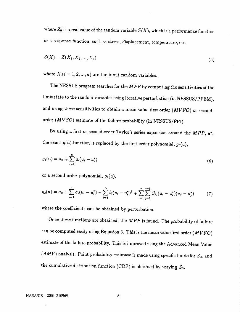
where Zo is a real value of the random variable Z(X), which is a performance function
or a response function, such as stress, displacement, temperature, etc.
z(x)-- z(xl,x2,...,x.) (5)
where Xi(i -- 1,2, ..., n) are the input random variables.
The NESSUS program searches for the MPP by computing the sensitivities of the
limit state to the random variables using iterative perturbation (in NESSUS/PFEM),
and using these sensitivities to obtain a mean value first order (MVFO) or second-
order (MVSO) estimate of the failure probability (in NESSUS/FPI).
By using a first or second-order Taylor's series expansion around the MPP, u*,
the exact 9(u)-function is replaced by the first-order polynomial, gx (u),
g,(u) = ao + F_. - ,<.) (6)i=l
or a second-order polynomial, 92(u),
n n n i--I
g2(u)-'ao+__ai(ui-u,)+_'_b,(ui-u*)2+_-'_'_C,j(ui-u_.)(uj-u_) (7)i=1 i=1 i=1 j=l
where the coefficients can be obtained by perturbation.
Once these functions are obtained, the MPP is found. The probability of failure
can be computed easily using Equation 3. This is the mean value first order (MVFO)
estimate of the failure probability. This is improved using the Advanced Mean Value
(AMV) analysis. Point probability estimate is made using specific limits for Z0, and
the cumulative distribution function (CDF) is obtained by varying Z0.
NASA/CR--2001-210969 8

Figure 2: Series System Structure
NESSUS/FEM employs innovative finite element technology and solution strate-
gies. It provides a choice of algorithms for the solution of static and dynamic prob-
lems, both linear and nonlinear, together with an interactive perturbation analysis
algorithm to evaluate the sensitivity of the response to small variations in one or
more user-defined random parameters.
NESSUS/FPI (Fast Probability Integrator) is used to evaluate structural response
cumulative distribution functions (CDF). There are two methods in the code, the
first-order reliability method and the advanced first-order reliability method. In gen-
era3, the structural performance or response functions (e.g., stresses, displacements,
vibration frequencies) are implicitly defined and each function evaluation may require
intensive computation. The AMVFO ( Advanced Mean Value First Order) method
reduces the computational burden and is the main probabilistic tool in NESSUS.
NESSUS/PFEM automates the AMV procedure by integrating the FPI code and
the FEM code.
NASA/CR---2001-210969 9

System and component-level failure modes
After the individual reliability analysis is completed, one then proceeds to the
system or subsystem level analysis. System failure may occur due to a combination
of any of the individual component failure modes. Many physical systems that are
composed of multiple components can be classified as series-connected or parallel-
connected systems, or combinations of series and parallel conditions. Descripticn of
these simple system structures is as follows.
• Series System
A system that is functioning if and only if all of its n components are functioning
is called a series system structure. Fig. 2 illustrates such a system.
If E_ denotes the failure mode i, then the failure of a series system is the event
E! = El U E2 U... U En
Then the failure probability of the system is
(s)
P! = P(E/) (9)
If each failure mode Ei is represented by a limit state g(X)" = 0 in basic variable
space, the failure probability can be obtained by the integration denoted as
P!= ]aex... f fx(x)dx (10)
NASA/CR--2001-210969 10

JointProbabilityDensityfx (x)
Xl
O
_//_'J Failure region: g(x) < 0
X 2
Figure 3: Basic reliability problem in two dimensions
NASA/CR--2001-210969 11

a
I
I
I
I
I
,1
b
Figure 4: Parallel System Structure
where X represents the vector of all the basic random variable (loads, material
properties, etc.) and f_ is the domain in X defining failure of the system.
This is defined in terms of the various failure modes as gi(X) < O. In two-
dimensional X space, expression (10) is defined in Fig. 3.
• Parallel System
A system that is functioning if at least one of its n components is functioning is
called a parallel system structure. A parallel structure of order n is illustrated in
Fig. 4.
NASAJCR--2001-210969 12

Figure 5: CombinedSystem Structure
In this case,the systemfailure event canbe written
E l = E1 N E2 _ ... N E_, (li)
• Combined Series-Parallel System Structure
This refers to systems which are a combination of series and parallel structures.
Fig. 5 shows an example of such systems.
The failure event of this system is written, for example, as
E] = [El n(E u E3)]u E_ (12)
It should be noted that not all engineering systems can be represented simply as
described above. Practical systems may be more complex and need more effort to
model.
NAS A/CR--2001-210969 13

System reliability computation
In NESSUS, two methods have been implemented for system reliability compu-
tation [4]: (1) probabilistic fault tree analysis combined with importance sampling
(Torng et al, 1992) and (2) a structural reanalysis procedure to accurately estimate
the failure regions for various critical failure modes affected by progressive damage
(Mahadevan et al, 1992).
Consider an engineering system subject to a sequence of loads (duty cycles) and
which may fail in any one (or more) of a number of possible failure modes under any
one load in the loading sequence. The total probability of the system failure may
then be expressed in terms of the individual mode failure probabilities as
Pi=P(E_)uP(E2nS_)uP(E3nS2n&)uP(E4nS3nS2nSl)U... (13)
where Ei denotes the "failure of the system due to failure in ith mode and Si denotes
the complementary "survival event of the ith mode.
Since P(E2AS1)= P(E_)- P(E2 n E_),..., Eq. 13 may be written also as
PI = P(EI)+ P(E2)- P(E, _ E2) + P(E3)- P(E_ N E3)
-P(E_ n Ea) + P(E1 n E2 n E3) + ... (14)
where (El n E2) is the event that failure occurs in both modes 1 and 2, etc.
Since it is not always an easy task to determine the joirtt probabilities of more
than two failure modes, the following approximation methods can be used to predict
the system reliabilities.
N AS A/C RI2_ 1-210969 14

• First-order bounds
The probability of failure for the system can be expressed as P; = 1 - P(S),
where P(S) is the probability of survival. For independent failure modes, P(S) can
be represented by the product of the mode survival probabilities, or, noting that
P(Si) = 1 - P(Ei), by
n
P! = 1 - H[1- P(E,)]i=I
(i5)
where, as before, P! is the probability of failure in mode i. This result can be shown
to be identical with Eq. 14. It follows directly from Eq. 14 that, if P(Ei) << 1, then
Eq.15 can be approximated by [Freudenthal et al., 1966]
PI = _ P(E,) (16)i=1
In the case where all failure modes axe fully dependent, it follows directly that the
weakest failure mode will always govern system failure, irrespective of the random
nature of the strength. Hence
Pf = m:ax[P( E,)] (17)
Equations 15 or 16 and 17 can be used to define relatively crude bounds on
the failure probability of any system of the series types when the failure modes are
neither completely independent nor fully dependent. These are Cornell's first-order
bounds:
n
max P(E,) < P(LJ,"__IE, ) < _ P(Ei) (18)l<i<n i=l
NASA/CR--2001-210969 15
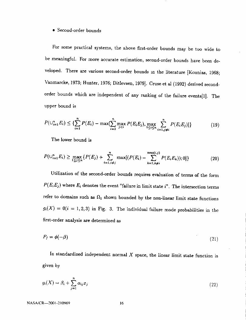
• Second-order bounds
For some practical systems, the above first-order bounds may be too wide to
be meaningful. For more accurate estimation, second-order bounds have been de-
veloped. There are various second-order bounds in the literature [Kounias, 1968;
Vanmarcke, 1973; Hunter, 1976; Ditlevsen, 1979]. Cruse et al (1992) derived second-
order bounds which are independent of any ranking of the failure events[l]. The
upper bound is
n n n
P(U'_=,E,) < {_.P(Ei) - max[__m<axP(EiEj), max __, P(EiEj)]} (19)i=l i----2 l<i<n-- i=l,j¢i
The lower bound is
n max(i,./)
P(UI"=,E,) > max{e(ES) + _ max[(P(E,)- _ P(EiEk));O]} (20)- i<j<_
i=l,i#j k=l,k#i
Utilization of the second-order bounds requires evaluation of terms of the form
P(EiEj) where Ei denotes the event "failure in limit state i'. The intersection terms
refer to domains such as fll shown bounded by the non-linear limit state functions
gdX) = O(i = 1, 2, 3) in Fig. 3. The individual failure mode probabilities in the
first-order analysis are determined as
Ps = (2i)
In standardized independent normal X space, the linear limit state function is
given by
n
yi(x) = + (22)j=l
NASA/CR--2001-210969 16

where n is the number of random variables.
The angle between the two limit states provides information about the correlation
of the two failure modes. The correlation coefficient is obtained as
n
Pij = E airajr -- COSVij (23)r=l
Once/3_,/3.i and PO are obtained, the computation of joint probability of failure
can be carried out. Eg. 19 and 20 can be used to compute the second-order bounds
for system failure probability estimation.
The above method only provides a tool to approximately estimate the failure
probability correlation of two different failure modes in a multi-discplinary system. A
more accurate approach would be the imposition of one failure mode on anther mode
and reanalysis of the latter. For example, consider two failure modes in a heat transfer
system: structural failure and heat transfer failure. Structural failure happens when
the stress, caused by the fluid pressure and temperature difference between outer and
inner surfaces exceeds limiting value of strength. The heat transfer failure happens
when the temperature of the contained liquid can not be kept at a certain level.
When the thermal failure occurs, the increase in the temperature field also causes
changes in stress field. The structural failure probabilty can be re-estimated under
this changed stress field and the result can be considered as the interactive failure
probability under influence of heat transfer failure. A numerical examples will be
shown for this approach in a later chapter.
NASA/CR--2001-210969 17

Symbol Meaning of symbol
Representation of an event
Representation of an event of a failure
OR-gate
AND-gate
Figure 6: Standard symbols used in fault tree analysis
Probabilistic fault tree analysis
NESSUS system risk assessment (SRA) uses probabilistic fault tree analysis
(PFTA). A fault tree is a mathematical construction of assumed component fail-
ure modes (bottom events) linked in series or parallel leading to a top event, which
denotes system failure. Standard graphical symbols are used to construct the fault
tree picture, by describing events and logical connections. These are shown in Fig.
6, and a simple PFTA is shown in Fig. 7.
• Fault Trees with a Single AND-GATE
Consider the fault tree in Fig. 8. Here the top event occurs if and only if all
the bottom events El, E2, ,.., En occur simultaneously. A system with AND-GATE
is very similar to a series system structure.
N AS A/C R--2001 -210969 18

57
4
o
_=! _3:.2
Figure 7: Probabilistic Fault Tree for System Reliability Example
NASA/CR--2001-210969 19

Symbols Description
AND-gate
The AND-gate indicates that the output
event A occurs only when all the input
events E i occur.
OR-gate
IThe OR-gate indicates that the output
event A occurs if any of the input events
E i occur.
Figure 8: Fault tree with a single AND-GATE and a single OR-gate
NASA/CR--2001-210969 20

I½
Figure 9: Schematic of NESSUS
• Fault Tree with a Single OR-GATE
Consider the fault tree in Fig. 8. The top event occurs if at least one of the
bottom events El, E2, ..., En occurs. The structure of this fault tree is similar to the
paralell system structure.
A schematic of Version 6.0 of the NESSUS (Numerical Evaluation of Stochas-
tic Structures Under Stress) probabilistic structural analysis computer program is
shown in Fig. 9. As shown in the diagram, the the NESSUS includes other modules,
namely the System Risk Assessment (SRA) and Simulation Finite Element (SIM-
FEM) modules. The random field pre-processor (PRE) provides data manipulation
needed to express the uncertainties in a random field as a set of uncorrelated random
variables. The user-subroutine which defines the response model (UZFUNC) enables
NAS A/CR--2001-210969 21

users to define required limit state with the computed response. This study will
mainly use FEM, PFEM and FPI for reliability analysis. The NESSUS program is
quite comprehesive with respect to structural reliability estimation. As mentioned in
Chapter I, the purpose of this study is to develop a technique by which the NESSUS
program can be used for the system reliability analysis of multi-discplinary systems.
The following chapters describe this technique in detail.
NASA/CR--2001-210969 22

CHAPTER III
ANALOGY BETWEEN ENGINEERING SYSTEMS
Introduction
Since NESSUS/FEM program has been mostly applied only to structural analysis,
a thermal or a fluid mechanical system needs to be converted through an analogous
model to a structural system on which the NESSUS program can be applied for
analysis. Then the probability analysis for a heat transfer system or a fluid mechanics
system can be carried out by NESSUS. By doing so, a system with heat transfer,
fluid flow and mechanical stress problems can be analyzed by NESSUS automatically
with FEM, PFEM, FPI and SRA modules for system reliability analysis.
In this chapter, a new methodology is presented for one-dimensional steady-state
heat transfer analysis and one-dimensional steady-state uniform flow problem using
a structural finite element program. First, the use of the analogous models is intro-
duced for the analysis of systems involving one-dimensional steady-state heat transfer
and simple one-dimensional steady-state uniform flow in closed conduit systems.
Heat transfer analysis through structural analogy
One-dimensional steady-state heat transfer
We begin our analysis of one-dimensional, steady-state conduction by discussing
heat transfer with no internal generation. The objective is to determine the expres-
sions for temperature distribution and heat transfer rate in common geometries.
NASA/CR--2001-210969 23

Y
qx
qy+dy
dx/
/ qz2 y /
qy
qz
/
%%
%
"_--- qx+dx
q generated within
volumn
" X
Figure 10: Differential volume for the derivation of the general equation of heatconduction
The concept of thermal conductivity (analogous to stiffness in stress analysis) is
introduced as an aid to solving conduction heat transfer problems. Consider a three
dimensional differential volume shown in Fig. 10, The general heat equation is
0 OT 0 OT 0 OT OT
-_x ( g -_x ) + _y ( K N) + -_z ( g _z ) + ?1 = P q, "-_ (24/
where K is the thermal conductivity of the material. K °T K °T K °T0N, 0r, a, are related to
heat flux in a direction perpendicular to the surface. _ is the rate at which energy is
generated per unit volume of the medium. The density p and specific heat % are two
thermodynamic properties. The product p% is the volumetric heat capacity, p%-g-?a:r
is the time rate of change of the internal (thermal) energy of the medium per unit
volume.
NASA/CR--2001-210969 24
Hot fluid
T_.1, hI
x
qx
Ts,2
T¢_,l Ts, l Ts,2 Too,2
qx ...._> _--/x/_-_JX/_/__
x=L
__..TT _, 2
TCold fluid
T_2 , h2
1 L 1
hiA kA h2 A
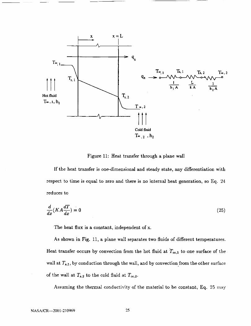
Figure 11: Heat transfer through a plane wall
If the heat transfer is one-dimensional and steady state, any differentiation with
respect to time is equal to zero and there is no internal heat generation, so Eq. 24
reduces to
d (KA_x ) 0 (25)
The heat flux is a constant, independent of x.
As shown in Fig. 11, a plane wall separates two fluids of different temperatures.
Heat transfer occurs by convection from the hot fluid at Too,l to one surface of the
wall at TsA, by conduction through the wall, and by convection from the other surface
of the wall at T_,2 to the cold fluid at T_oa.
Assuming the thermal conductivity of the material to be constant, Eq. 25 may
NASA/CR--2001-210969 25

be integrated twice to obtain the general solution
T(x) = C,z + C2 (26)
To obtain the constants of integration, CI and C2, boundary conditions must be
introduced. These are:
T(O) = To,1 (27)
T(L) = T,a (28)
Applying the condition at x = 0 to the general solution, it follows that
Ts,,= C_ (29)
Similarly, at x = L
Ts,2 = C1L + C_ = C, L + T,,1 (30)
in which case
T, a - Ts, 1= C1
L
Substituting into the general solution, the temperature distribution is then
IN, }where N, = 1 - z, N2 = Z_
The heat flow can be determined by Fourier's law, that is
KA dTq=- _x
(31)
(32)
or
q = -KA " (T,i T_)] = KAL(T1- V_) (33)
NASMCR--2001-210969 26

F
fl, U1
1
"'- r
X,U
D
2
q
=!
F
f
f2,U2
Figure 12: Bar subject to tensile force F
Stress analysis of a bar element
Now consider a linear-elastic, constant cross-sectional area (prismatic) bar element
shown in Fig. 12. Using Hooke's law, the differential equation governing the linear-
elastic bar behavior is
d"_ k _] = 0 (34)
where U is the axial displacement function in the x direction and S and E are
cross-sectionM area and Young's modulus of elasticity respectively.
cN,where N1 = 1 - _, and N2 - _
The strain-displacement relationship is
dU Us - U1E+ - - (35)
dx D
NASA/CR--2001-210969 27

Table i: Analogous quantities for structural and thermal systems
Heat flux q I Nodal force fl
Temperature T( x )
Inverse of heat transfer resistance
Conduction: gL-4, convection: hA
Displacement U(z)
Structural stiffness B._5_sD
We obtain
F = ES ( U2-Ux )D
Also, by the nodal force sign convention of Fig. 12,
(36)
ft = -F (37)
So Eq. 36 becomes
f, = - v2) (38)
Analogous modeling between heat transfer and structure
Comparing Eq. 38 with Eq. 33, the similarities become apparent. These two
equations indicate a direct analogy between heat transfer and structural analysis.
The analogous quantities are listed in the Table 1.
With this analogy, we are able to model a he_t transfer problem into a stress
analysis problem.
NASA/CR--2001-210969 28

In the plane wall, we refer heat transfer resistance of conduction R to K_A, that
is
Tsl -Tsa LRcond -- ' (39)
q KA
Considering the structural system, Hooke's law provides stiffness of the form
fl _ E____S (40)U1 - U2 D
Comparing Eqns. 39 and 40, and considering gL-4 and --_ as analogous qualities,
1
R,:onatcan be traced to be analogous to K.
A heat transfer factor may also be associated with convection at a surface. From
Newton's law of cooling,
q=hA(T,-Too) (41)
where h is Planck's constant of convection heat transfer coefficient, Ts is the surface
temperature and Too is the ambient temperature.
The thermal resistance for convection is then
R_o,_ - Ts - Too _ 1__ (42)q hA
The equivalent thermal circuit for the plane wall with convection surface condi-
tions is shown in Fig. 11. The heat transfer rate may be determined from seperate
consideration of each element in the network, that is,
KA (T,,I - T,a)= h2A(T,,2- Too,2)q = h,A(T,:,¢,,- Ts,,) = T
(43)
NASA/CR--2001-210969 29

In terms of the overall temperature difference, To_,l - Too,2, and the effective
thermal resistance R_lf, the heat transfer rate may also be expressed as
T_,I - T_,2 (44)q = Reff
Because the conduction and convection resistance are in series and may be summed
up, it follows that
1 L 1
Refl "- h_A + "_ + h2A (45)
Consider a bar consisting of three different materials which are denoted as ele-
ments 1,2 and 3. The effective stiffness for this composite bar is
1
k_:!= I + 1 1 (46)kS _+_
Comparing the above equations Eq. 45 and Eq. 46, the analogy is k,/! +--+ n-_,1'
that is
1 1 1
noz _ y, + _ + k--; (47)
Substituting with Eq. 45, we obtain
1 L 1 1 1 1
h,---_+ _-_ + _ _ _ + _ + k-_ (48)
where
E1S1k, = _ (49)
D1
E2 _qlk_ = (50)
D2
E3 S_k3 = _ (51)
D3
NASA/CR--2001-210969 30

Substituting the correspondingterms in Eq.48,weobtain the equivalent quanti-
ties
(D_)_E1 4---+ (hlA) 7- (52)
E3 +---+ (h2A) _ (54)
With these analogous quantities, we use the NESSUS/FEM beam element with
the E values replaced by the values involving heat transfer problem outlined above.
The boundary conditions for the bar are the end displacements corresponding to the
ambient temperature of the wall. After the structural analysis, we get the tempera-
ture distribution from the corresponding displacement distribution in the output.
Heat transfer in composite walls
Equivalence concepts for thermal-structural analysis may also be used for more
complex systems, such as composite walls and radial heat transfer systems. Fig. 13
shows a series composite wall. The one-dimensional heat transfer rate for this system
can be expressed as
T ,I - T ,4 (55)q= Y']_R
where T_,I - T_,4 is the overall temperature difference and the summation includes
all thermal resistances. Hence
NAS A/CR--2001-210969 31

T=,I
T_, 1, h 1
Hot fluidTs,4
\ T_,4
Cold fluid
1 1 1 1 1
h iA kAA kBA kcA h4A
q___>o._A A _.o_._ A A/x_o_.A A A/-cm/W___T=,I T3 Ts,4 T=,4
Figure 13: Equivalent thermal circuit of a series composite wall
N AS AJCR--2001-210969 32

t kl k2 k3 k4 k5
1@+2@+3@+4@+5@+6
Figure 14: Structural analog for the series composite wall heat transfer
Too,l - Too,4
q = RI+R2+R3+R4+Rs(56)
Tco,l - Tco,4
(1/h,A) + (LA/KAA) + (LB/KBA) + (LB/KsA) + (1/h4A)(57)
Alternatively, the heat transfer rate can be related to the temperature difference
and resistance associated with each element. For example,
Too,l - Ts,l Ts,1 - T2 T2 - T3 - (58)q-- (1/h_A) (LA/KAA) (Ls/KBA) "'"
The analogous structural model for this series composite wall heat transfer prob-
lem is shown in Fig. 14. The bar consists of five elements with stiffnesses of
kl, k2, k3, k4, ks. Using the mechanical structure equivalence for convection and con-
duction, we obtain
E = { (hlA)(D) for convection }for conduction
NASA/CR--2001-210969 33

Engine oil
T_..i, h2
Outer pipe/ fJ_" ! (_L'_ '_ _ _ - - -
" _ I_ q_ l .ln(rl/r2) !Refridgerant TJ,2Inner duct h 12 rlL 2 kL hz 2 r2 L
(a) Heat exchanger
, o,t, @,t, o _,
(b) Structural model
Figure 15: A heat exchanger for engine oil and refrigerant fluid
NAS A/CR--2001-210969 34

Heat transfer in radial systems
Cylindrical and spherical systems often experience temperature gradients in the
radial direction only and may therefore be treated as one dimensional.
Fig. 15 shows an example of a heat exchanger, whose inner cylinder is used to
store engine oil and the outer cylinder is used to transfer the refrigerant fluid to
cool down the oil temperature. The outer insulated covering is assumed to isolate
the system from the ambient environment. For steady state conditions with no heat
generation, the appropriate form of the heat equation is
1 d (KrdT_rdr \ _] =0 (59)
The rate at which energy is conducted across any cylindrical surface in the solid
may be expressed as
-KA dT - g(27rrL)-_- (60)q= dr =
where A = 2_rrL is the area normal to the direction of heat transfer.
The thermal resistance is
11 ln(r2/rl) + (61)
R_]f - h12zrrlL + 27rKL h22zrr2L
which includes both conduction and convection.
The heat transfer rate for a unit length of the cylinder therefore is
Too,1 - Too,2q = (62)
i +_+ ihl2rrlL 21rKL h221tr_L
NASA/CR--2001-210969 35

Table 2: Analogous quantities for heat transfer in a radial system.
Structure Heat transfer
El
E2
E3
The structural analog for the cylinder is shown in Fig. 15(b). In this case, the
mechanical structure equivalence is k,ll +---+ 1 The corresponding equivalentRel! "
quantities are listed in Table 2. The E values are input to NESSUS structural anal-
ysis, and the output displacements from NESSUS give the temperature distribution.
Numerical example for heat transfer solved with NESSUS/FEM
Fig. 17 shows the sectional view of the cylindrical copper heat exchanger which
the engine oil flows through. The copper wall thickness is 0.281 in. The radius
to the surface of the insulation pipe covering (ki = 0.428Btu/(h - ft 2 o F)) is
1.33 in. The fluid in the outer container is controlled at a constant temperature
of 70°F. The forced convection heat transfer occurs between the outer surface of
the insulation covering and the flowing fluid with h = lOBtu/(h - ft 2 -° F). The
surface temperature at the insulation covering is 35.298°F. The structural analogy
model is used to determine the inside temperature of the tube, assuming steady
state, one dimensional, uniform properties in each material, forced convection cooling
and negligible thermal radiation. The conductivity coefficient of copper at room
NASA/CR--2001-210969 36

TF= 70°F Rkl 7"1
qf
R k2 T2 R c 7"3- 5°F
(a) Thermal circuit
k3= _S3/D3 kl= _ S1/D 1
, G o ,f ,G_- k2= S2/t Y
F
(b) Structural analogous model
Figure 16: Analogous model for the heat exchange
temperature is Kc = 223Btu/(h - ft 2 -° F).
The thermal circuit is shown in Fig. 16(a). Fig. 16(b) shows the structural
analog model for this heat transfer problem. Beam element type 98 in NESSUS/FEM
element type library is adopted. Three elements represent three heat transfer forms
involved in this problem, which are the forced convection between the surface of
the insulation covering and the ambient air, conduction through the copper layer,
and conduction through insulation covering, respectively. Therefore, in terms of the
structural model, we must assign three different material elastic constants for this
beam structure. Since the NESSUS/FEM utilizes the Nodal-based data input, two
duplicate nodes are used at each boundary between elements 1 and 2, and between
elements 2 and 3. The room temperature 70°F becomes the boundary displacement
NASA/CR--2001-210969 37

T, T__. T_ _ ro = 1.330 in
r1 = 0.669 in
r2 = 0.950 in
T® = 70°F
= 10 Btu/(h- ft 2-°F)
Insulation Copper k = 0.428 Btu /(h - ft 2. OF)
covering duct
Figure 17: Section of a radial heat exchanger
70.0 at node 1. A concentrated load F at point 3 is -241.66 lb. The length of the
structural element is 10.0 units, the sectional area is 1.0. It should be noted that the
units used in the structural model here do not have any real meaning in terms of a
real structure. They are simply used to facilitate the structural analysis.
The equivalent values are calculated as follows.
E, = ln-(-;_,)] _ = 1n(0.95/0.669)× 10= 3995_.476 (63)
E2 = tln(r0/r2)] -_2 =2_r x 0.428
In(1.33/0.95) x 10= 79.923 (64)
(65)
F = 2_rroh(T_ - T_) = 2rr x 1.33/12 × 10(35.298 - 70) = -241.66 (66)
N ASA/CR--2001-210969 38

NESSUS/FEM uses this data, and gives the output of the displacement distribu-
tion in the structure as follows:
U1 = 70.000
0"2 = 35.298
U3 = 35.298
0"4 = 5.0614
/-)'5 = 5.0614
U6 = 5.0009
Converting the above displacement information to the equivalent temperature
distribution, we obtain:
T_ = 70.000°F
T1 = 35.298°F
T2 = 5.0614°F
T3 = 5.0009°F
The data and the output files are shown in Appendix A.
Fluid flow analysis through structural analogy
Equation of motion for fluid flow
The Bernoulli equation gives a relationship between pressure, velocity, and posi-
tion or elevation in a flow field. Normally, these properties vary considerably in the
flow, and the relationship between them if written in differential form is quite com-
plex. The equation can be solved exactly only under very special conditions. There-
NASAJCR--2001-210969 39

Pl
! L !
Figure 18: Fluid in a constant diameter duct
fore, in most practical problems, it is often more convenient to make assumptions to
simplify the descriptive equations. The Bernoulli equation for steady, incompressible
flow along a streamline with no friction (no viscous effects) is written as [10]
V 2P + + gz = C (67)p -Y
where
p is fluid pressure
p is the desity of the fluid
V is the flow velocity
g = 32.174 ft/s 2, and z is height.
For a horizontal pipe shown in Fig. 18, zl = z2. From continuity, A1V1 = A2V2.
Because D1 = D2, then A1 = A2, and therefore, Vx = V2. T1/e Bernoulli's equation
reduces to
Pl = P_ (6S)
NASA/CR--2001-210969 40

"¢w Pdz
......-_! .4..--
pA--" i "-- (p+dp)A
Figure 19: Control volume of a system: flow in a duct.
This result is not a proper description of the situation, however. For flow to be
maintained in the direction indicated in Fig. 18, Pi must be greater than p_ in an
amount sufficient to overcome friction between the fluid and the pipe wall. In order
to apply Bernoulli's equation and obtain an accurate description, we must modify
the equation with a friction term.
Consider flow in a pipe as shown in Fig. 19. A control volume that extends to
the wall (where the friction force acts) is selected for analysis.
Note that a circular cross section is illustrated, but the results are general until
we substitute specific equations for the geometry of the cross section. The forces
acting on the control volume are pressure normal to the surface and shear stress
acting at the wall. The momentum equation is [10]
(69)
NASA/CR--2001-210969 41

where
V. is the fluid velocity along the longitudinl direction
V_ is the norminal fluid velocity
Since the flow out of the control volume equals the flow in, the right-hand side
of this equation is zero. The sum of the forces is
pA - r_Pdz - (p + dp)A = 0 (70)
where
A = cross-sectional area
Pdz = the surface area (perimeter times length) over which the
wall shear r_ acts
The equation reduces to
r,_Pdz + Adp = 0 (71)
Rearranging and solving for pressure drop, we get
dp = _4rw (72)dz Dh
We have thus expressed the pressure drop per unit length of the conduit in terms
of the wall shear and the hydraulic diameter. Eq. 72 is a general expression for any
cross section. It is convenient to introduce a friction factor f, which is customarily
defined as the ratio of friction forces to inertia forces:
4ru_
f_ __pl/2 (73)2
NASA/CR--2001-210969 42

Figure 20: Laminar flow in an annulus
where V is the average flow velocity.
By subsitution into Eq. 72, we obtain
pV 2 f dz (74)dP=-2 Dh
Integrating this expression from point 1 to point 2 a distance L apart in the
conduit yields
V2 2Dh A- (75)
Eq. 75 gives the relationship between the velocity and the pressure drop in the
duct due to friction. This equation can be applied to two flow regimes- laminar and
turbulent flow. However, caution must be excercised when determining the friction
factor f.
This equation can also be applied to flow through noncircular cross section such
as rectangular duct and annulu_ Fig. 20 shows the laminar flow in an annulus.
NASA/CR--2001-210969 43

Table 3: Analogous quantities between structural and flow systems
]1 Fluid mechanics Structure 1]
Square of velocity V 2 Nodal force ]'1 = -F
Pressure distribution p(x) Displacement U(x)
Flow factor 2_D Structural stiffness -_pIL
The annulus flow area is bounded by the inside surface of the outer duct (radius
R1) and the outside surface of the inner duct (R2). We define the ratio of these
diameters as
k = --R2 (76)Rt
in which 0 < k < 1.
The friction factor used in Eq. 75 is defined as [10]
1 Re [1 + k 2 1 + k] (77)7= 64 []--T¢ +ln(k) j
where R, = Pv-KiL_(1 - k).
Compare Eq. 75 with Eq. 38 concerning the beam structure subjected to the
end nodal force, as discussed in previous section:
A = - g2) (78)
We are now able to set up the analogous quatities listed in Table 3.
NASA/CR--2001-210969 44

Numerical example of flow in a tube solved with NESSUS/FEM
Consider the refrigerant flow in a copper tube as an example to demonstrate how
NESSUS/FEM can be applied to problems in fluid mechanics.
A horizontal copper duct as shown in Fig. 18 with inside radius of 0.669 in, and
1,200 in in length. If the inflow pressure pl is 1838.7 psi, assuming the refrigerant
is Freon F-12 under a temperature of 5°F, p is 0.0499 lb/in 3. The friction factor f
is assumed to be 0.03, and V is 15.5 in�see. The objective is to obtain the outflow
pressure p_ using NESSUS/FEM.
First of all, we need to identify all the equivalent quantities for structural analysis.
We assume a single element beam structure subjected to a concentrated force equal
to -240.25 units. The beam element has a section of 0.1 inx 0.1, and a length of 1.0.
The boundary condition is an initial displacement of 1838.3 units at node 1. Again,
it should be mentioned that the units used here do not have real meaning in terms
of a real structure. According to Table 3, the analogous quantities can be obtained
as follows
E = _,p--_/ = 0.0499 x 0.03 x 1200 x 10 = 14.896
f, = V 2 = 15.52 = 240.25
F = -240.25
This data is input to NESSUS/FEM, and the displacement at point 2 is ob-
tained as 1677.4. Converting this displacement to the fluid model, we get the output
pressure P2 = 1677.4 psi.
The data and the output files are shown in Appendix B.
NASA/CR--2001-210969 45

CHAPTER IV
MULTI-DISCIPLINARY SYSTEM RELIABILITY ANALYSIS
Introduction
After transforming the heat transfer and fluid mechanics problems into corre-
sponding structural analog models and using NESSUS/FEM to perform the finite
element analysis, we can define the individual failure modes in NESSUS/FPI. Then
NESSUS/PFEM can be employed to integrate FEM and FPI programs to obtain
the failure probability and CDF for each failure mode. The failure mode for heat
transfer problem would be defined as, for example, the event that the temperature
at a certain location is lower or higher than the required temperature. The failure
mode for fluid flow would be defined as the flow pressure exceeding a certain pressure
level, and the structural failure is defined as the stress exceeding either the ultimate
strength or the yield strength of the material.
Upon the completion of failure probability analyses of individual failure modes,
the system failure analysis can be pursued. The different failure modes involved in
a system have different impacts on the overall performance of a system. Some types
of failure such as structural failure are critical to the system. If the material used to
construct the main parts of the system fails, the whole system can no longer function.
Such failure is called critical failure. Other failures modes such as thermal failure of a
heat exchager do not destroy the system bu_ degrade the performan _c of the system.
NASA/CR--2001-210969 47

Such failure is referred as to functional failure. The function of fluid flow will fail
when the outflow pressure rises higher than the designed value, but the system can
still be working until the pressure increases to the level which will cause the system
to shut down. The individual failure modes can also be correlated to each other. For
example, the temperature field in the thermal failure mode affects the stress field in
the structural mode. The flow pressure definitely has impact on the stress. However,
in some cases, the component-level events in a system is considered as independent
events. In the example which will be discussed later in this chapter, the thermal
failure and fluid flow failure modes do not share correlated input parameters, so they
are considered as independent of each other.
Using the analogy method, the thermal and fluid flow problems are analyzed sim-
ilar to the structural model by means of NESSUS. For physically correlated events,
the failure mode of one event is imposed on the other. In a system consisting of
structural, thermal and fluid flow modes, the thermal and flow failures are imposed
into the structural failure analysis to study the impact of correlated events. The
failure probability of the whole system is then estimated based on the output from
the above analyses.
Individual failure analysis
Structural failure mode
For a copper duct of a heat exchanger shown in Fig.17 in Chapter III, the
structural failure mode is defined as that when the tensile stress exceeds the yield
strength f_i_14 = 8.0 ksi. In finite element modeling, we use Element type 153 in the
NESSUS/FEM file. This element is a four-noded quadrilateral lying in the global
NAS A/CRy2001-210969 48

zr-plane which is defined by cylindrical coordinates.
This structure is subjected to two types of load - fluid pressure from the inside
flow and the stress caused by temperature difference between the outer surface and
the inner surface.
One convenient feature of the NESSUS/PFEM is that we can impose different
temperatures at the inner surface of the pipe and obtain the different probability
results under different temperature conditions. This enables us to investigate the
effect of different temperature levels on the structural failure probability. By doing
so, the relationship between the failure modes in two dicsiplines - heat transfer and
structural mechanics - is established. This is a significant step toward the system re-
liability analysis with physically correlated failure modes. This will be demonstrated
in a later section.
For this structural failure model, we first suppose that the temperature failure
(which will be descibed in the following section) did not occur, that is, the tempera-
ture at the inner surface of the duct is below 5.0009°F. Given that the inner surface
temperature is 4.0000°F, using the FEM we obtain the outer surface temperature as
4.0605°F.
Also, we assume that the outlet flow pressure is under 1677.4 psi which enables
the system to work properly. We assume that the outlet flow pressure is 1577.4 psi.
We input this temperature and flow pressure profile in the structure FEM data
file, with the random variables defined in Table 4.
NASA/CR--2001-210969 49
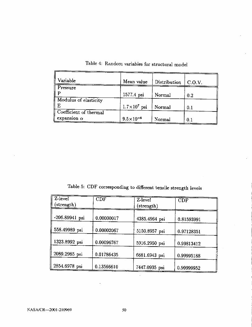
Table 4: Random variables for structural model
Variable Mean value Distribution C.O.V.
Pressure
P 1577.4 psi Normal 0.2
Modulus of elasticity
E 1.7x10 r psi Normal 0.1
Coefficient of thermal
expansion a 9.5 x 10 -8 Normal 0.1
Table 5: CDF corresponding to different tensile strength levels
Z-level CDF Z-level CDF
(strength) (strength)
-206.89941 psi 0.00000017 4385.4964 psi 0.81593991
558.49989 psi 0.00002067 5150.8957 psi 0.97128351
1323.8992 psi 0.00096767 5916.2950 psi 0.99813412
2089.2985 psi 0.01786435 6681.6943 psi 0.99995188
2854.6978 psi 0.13566610 7447.0935 psi 0.99999952
NASA/CRy2001-210969 50

The result attached in Appendix C indicates that the structural reliability when
the heat exchanger is working properly in thermal and fluid aspects is 0.99999999.
The failure probability is expressed as 1 - Pr,,_b_tit_. Therefore, the structural failure
probability is 1.0 × 10 -9.
The key word response type in the NESSUS input data file, FPI section, is set
equal to 3 which means that the response quantity used in limit state function is
stress. The corresponding keyword analysis type in FPI section is first set equal to
1 which means that the probability analysis is for a single Z-level. The Z-level in this
case is 8,000 psi. The probability result will be under the condition of a < 8,000
psi, i.e., the structural reliability of the system under certain thermal and fluid flow
working conditions.
The CDF is obtained by using PFEM by setting analysis type in FPI section
equal to 0 which automatically generates a set of different values of Z0 (i.e., Z levels
for a series of stress valus) for probability analysis. The CDF values corresponding
to different strength Z-levels are shown in Table 5.
The CDF chart is shown in Fig. 21. It should be noted that the first line of
the data which contains negative Z-level is eliminated because negative stress is
considered impractical in this model. The input and output files are attached in
Appendix C as well.
NASA/CR--2001-210969 51

r.9
1.0
0.8
0.6
0.4
0.2
0.00.0
I
I
2000.0 4000.0 6000.0
Strength levels (psi)
8000.0
Figure 21: CDF of structural reliability of refrigerant duct
Table 6: Random variables for thermal model
Mean value Distribution Coefficient of variation
K_ 223.0 Normal 0.1
Ki 0.428 Normal 0.1
h 11.3 Normal 0.1
N ASA/CR--2001-210969 52

1.0
0.8
0.6
0.4
0.2
0.0--40.0
1 ' I ' I
, 1 I
-20,0 0.0 20.0
Internal fluid temperature levels ( °F )
40.0
Figure 22: CDF of internal fluid temperature of refrigerant duct
NASA/CR--2001-210969 53

Failure mode in heat transfer
Using the same example of a heat exchanger as in Fig. 17, we define a failure
event when the inside temperature is higher than 5°F, because the refrigerant will
not function properly beyond 5°F which is considered as a failure in the device we
studied. First the input data for NESSUS/PFEM is set up to obtain the reliability
under this failure mode, then the data file is set up with different Z - levels to obtain
the CDF, which provides reliability estimatecorresponding to different temperature
levels. The random variables Kc and Ki and h for heat transfer are defined in Table
6.
In order to use NESSUS/PFEM, the analogous quantities El, E2, E3 and F
are calculated from Eqs. 63, 64, 65, 66. Because the distribution of the random
variables Kc and Ki and h is normal and El, E2, E3 are linear to K_ and Ki and
h, the distribution of random variables El, E2, E3 is also normal. The mean values
and standard deviations of of El, E2 and E3 are input to NESSUS/PFEM.
The Z-level is 5.0°F, so P(Z < Z0) is the probability the device can keep the
inside fluid temperature under 5.0°F, which is the thermal reliability of the system.
We set up the keyword in FPI section analysis type equal to 1 which means the
probability analysis is performed for a single Z-level. The result is attached in Ap-
pendix D. The thermal reliability of this device is 0.9099214. Therefore, the thermal
failure probability is 9.00786 x 10 -2.
The CDF is obtained by setting up the FPI keyword analysis type equal to 0
which automatically generates a set of different values for Zo (i.e., Z-levels). The
NASA/CR--2001-210969 54

Table 7: Random variables for flow model
Mean value Distribution Coefficient of variation
Dh 0.669 Normal 0.1
V 18.71 Normal 0.1
CDF output is shown in Appendix D and the CDF curve is shown in Fig. 22.
Failure mode in fluid flow
Next we consider the one-dimensional fluid flow in a duct of a heat exchanger.
The failure mode is defined as the pressure at a certain point along the duct rising
above the value at which the system cannot function properly.
The example of a duct in a heat exchanger shown in Fig. 16 is used. The only
difference is that V is assumed to be 18.7 in/sec. We define the failure mode when
pressure rises above 1677.4 psi. The Z-level is therefore 1677.4 psi. The keyword
response type is set as 1 for the displacement output which is the analogy of the
pressure. The random variables related to fluid flow are defined in Table 7. The
analogous quantities for use in NESSUS/PFEM are calculated according to Table 3
as follows:
(2Dh _ 2 × 2 × 0.669
0.0499 × 0.03 × 1200x i0 = 14.896
fl = V 2 = 18.72 - 350.0
P = --fx = -35o.o
NASA/CR--2001-210969 55

1.0
0.8
0.6
0.4
0.2
I
J I !i
1500.0 1600.0 1700.0
Outlet fluid pressure levels (psi)
i
1800.0
Figure 23: CDF of fluid pressure of refrigerant in the duct
NASA/CR--2001-210969 56

Since E is a linear fuction of Dh, its distribution is also normal. But since fl = V 2,
the distribution of fl is actually chi-square (X2). However, we have used the normal
distribution for fl in this study as an approximation. The friction fator f is assume
to be a constant.
A NESSUS/PFEM input data file is compiled. The reliability is obtained by
setting the keyword analysis type equal to 1, and the CDF is obtained by setting it
to a value of 0 which automatically generates a set of different values for Zo. The
PFEM input and output files are shown in Appendix E and the CDF curve is shown
in Fig. 23.
The reliability is 0.98670241 and therefore the failure probability of the output
flow pressure being higher than 1677.4 psi is 1.329759 × 10 -2.
Multi-disciplinary system reliability
After the individual failure modes are identified and analyzed, the system reli-
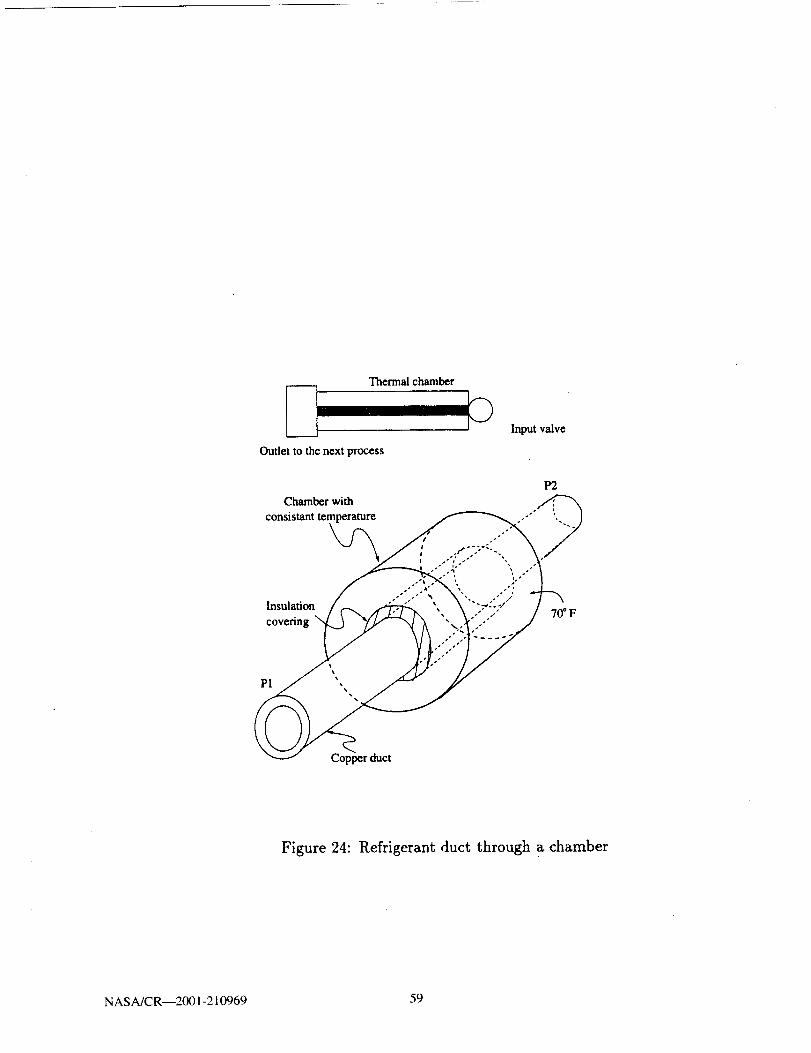
ability analysis can be pursued. Fig. 24 shows a device which is used to transfer
refrigerant fluid through a copper duct. The duct is installed in an enclosed cham-
ber which is maintained at a constant temperature of 70°F. The thickness of the
copper wall is 0.281 in. The radius to the surface of the insulation pipe covering (
mean value of K_ equals to 0.428 Btu/(h - ft 2 o F), c.o.v, equals to 0.1 ) is 1.33
in. Forced convection heat transfer occurs with h = lOBtu/(h - ft 2 o F) ( mean
value with c.o.v, equals to 0.1). The thermal conductivity of copper Kc has a mean
value of 233.0 Btu/(h - ft 2 o F) with a c.o.v. 0.1. The surface temperature at
the insulation covering is 35.298°F. The inflow pressure Pl is designed to be 1838.7
NASA/CR----2001-210969 57

psi. The refrigerant is Dichlorodifluoromethane ( Freon F-12 ) under a temperature
of 4°F. p is 0.0499 lb/in z. The friction factor f is assumed to be 0.03, and V is
18.71 in/sec ( assuming V 2 is normal distribution and has a c.o.v, of 0.1). The inner
radius of the duct has a mean value of 0.669 in and a c.o.v, of 0.1.
The above data are the same as the model shown in Fig. 17 of Chapter III, which
are used in FEM analysis and reliability estimation of individual failure modes. The
system shown in Fig. 24 is simply the combination of the previous individual models
which have been analyzed in different disciplines. The following is to demonstrate
how the analysis results of the individual failure modes can be integrated into the
analysis of a whole system.
The failure of the system consists of the individual failure modes in three disci-
plines: structural failure, thermal failure and fuid mechanics failure.
• First of all, the duct should work without any damage to the structure, i.e. the
duct should be structurally sound without yied or crack. If yield occurs, then
structural failure is assumed to occur. We denote the structural failure as El.
The structural failure is a critical failure in this system.
• The refrigerant liquid this device transports is sensitive to temperature changes.
The requirement is that the temperature cannot be higher than 5°F for the
next process to proceed. If the temperature of the liquid rises higher than 5 0 F,
then thermal failure occurs, which we refer to as E2. The thermal failure is a
non-critical functional failure in this system.
• It is required that the fired flow be maintained zt a certain presure at the
NASA/CRy2001-210969 58
Thermal chamber
Input valve
Outlet to the next process
P2
Chamber with
consistant te --.
PICopper duct
Figure 24: Refrigerant duct through a chamber
NASA/CR--2001-210969 59

ends which enables the refrigerant fluid to maintain a steady speed to provide
constan volume in the device. If the flow pressure rises higher than 1677.4
psi, the flow failure occurs, which is referred to as E3. The flow failure is a
non-critical functional failure in this system.
From the previous section, the probability of the individual failure modes of _he
system shown in Fig. 24 have been obtained, wich are:
P(Ex) = 1.0000000 x 10 -9
P(E2) = 9.0078600 x I0-_
P(E3) = 1.3297590 x 10 -_
As was indicated in the previous section, we can also impose one failure mode
upon the other. In this case we can impose the thermal failure ( which happens
when the fluid temperature rises above 5°F ) and the fluid pressure failure ( which
happens when the outlet fluid pressure rises above 1677.4 psi) upon the structure
respectively. In the FEM file for the structure model, the corresponding data are
modified to impose those failures.
First, we assume that the temperature failure occurs while the fluid pressure is
still lower than 1677.4 psi, say 1577.4 psi, i.e., the fluid flow is operation in safe mode.
By redefining the temperature profile in the FEM data deck as 6.06°F (for example)
in the inner layer of the wall and 6.12°F in the outer layer of the wall, which mean the
thermal failure occurs, we inpose the thermal failure to the structural model. The
PFEM result gives us the structural failure probability under the condition that the
thermal failure occurs. In this case, the structural reliability is 0.99999996, therefore,
NASA/CR--2001-210969 60

the failure probability P(Ex/E2) = 4.0 x 10 -s.
Now we impose the fluid pressure failure upon the structural model. The fluid
mechanical failure occurs when the pressure at the outlet rises above 1677.4 psi, say
1777.4 psi. The structural FEM file is modified by redefining the pressure profile
according to this failure pressure. It should be noted that the temperature profile
should remain under the normal working condition, which is that the temperature
in the inner layer of the wall of duct is under 5°F, say 4°F, i.e., the thermal as-
pect of the system is operating in the safe zone. The result indicates that in this
case, the structural reliability is 0.99999633, therefore, the conditional probability,
P(E1/E3) = 3.67 × 10 -6.
Next, both thermal and fluid mechanical failures are imposed that is, the fluid
temperature rises above 5°F, and the outlet flow pressure rises above 1677.4 psi.
Modifying the input FEM data deck in structural PFEM file with inner surface
temperature of 6.06°F, and the fluid pressure of 1777.4 psi, we can get the result of
the structural reliability of 0.99999227, which means, P(E1/E2E3) = 7.73 × 10 -6.
The conditional probabilities of structural failure have been obtained as
P(EI/E2) = 4.00 × 10 -s
P(E1/E3) = 3.67 × 10 -s
P(EI/E2E3) = 7.73 × 10 -6
System reliability computation
System reliability analysis can be performed in two different ways, depending on
the definition of the system failure. In the first (traditional) method, we define that
NASA/CR--2001-210969 61

Structural
Failure
System Failure
I
?GThermal Fluid flow
Failure Failure
Figure 25: Fault tree for the system with three critical failures
the system failure occurs when any component-level failure occurs. In the system
invoving structural, thermal, fluid mechanical failure modes, i.e., El, Ez and E3, the
system failure can be illistrated in a fault tree shown in Fig. 25.
As discussed in Chapter II, the probability of system failure P(E) can be obtained
using the following equations:
P(E) = P(Et U E2 t.J E3) (79)
The above expression can be expaned as:
P(E) = P(EI) + P(E2) - P(EI fq E2) + P(E3) - P(Et n E3)
-P(E2 n E3) + P(E_ n E.n E3) (80)
Since the joint probability is not always available, an approximate method is to
consider the individual failure modes as independent and ignore the correlations. In
our case however, the conditional probabilities have been calculated. Therefore_ the
N ASA/CR--2001-210969 62
systemfailure probability can be computedas
P(E) = P(E1) ÷ P(E2) -4- P(Ea)- P(E,/E_)P(E2)- P(E1/E3)P(E3)
-P( E2/ E3)P( E3) -4- P( EI/ E2Ea)P( E2E3) (81)
For systems involving many failure modes, approximation methods are used to
predict the system failure probability (or reliability), such as first-order bounds or
second-order bounds [1].
Since no correlation is assumed between the failures of flow pressure and fluid
temperature, we assume P(E2 f3 E3) is equal to P(E2)P(E3) in our analysis.
Substituting the numerical results from the previous discussion into Eq. 81,
we obtain the probability of the system failure of the heat exchanger, P(E) =
0.10217832.
As mentioned before, the above failure probability is an estimation of system
failure in case any failure occures which includes both critical and non-critical func-
tional failures. Now we will pursue the probability estimation for the system critical
failure which, in our case, is structural failure. During the service cycles, the thermal
and fluid mechanical failures may be non-critical, i.e., their occurence does not cause
total system failure. They will cause the system to fail in some functions as designed,
such as keeping the fluid under certain temperature or keeping the outlet fluid pres-
sure under certain value. However, if the the system keeps operating, the changes in
temperature and fluid pressure will cause progressive damage to the structure due
to load redistribution. The estimation of critical structural failure of the system has
to consider the progressive damage caused by all components. Structural reanalysis
NASA/CR--2001-210969 63

Table 8: Structural failure probability under various temperatures
T(°) 0.0 5.0 102 15.0
P( E1) 0.0 0.0 0.0 0.0
is used to account for the effect of non-critical d_mage on critical failure mode. In
the refrigerant model, a reanalysis procedure is performed to accurately estimate the
failure region segments for structural failure mode affected by progressive damage
caused by thermal and fluid pressure changes within the system. The overall struc-
tural failure probability is obtained through the union of the failure region segments
defined by each limit-state function.
We can also impose a series of temperatures under which the system may be
operating upon the structural model to examine the temperature impact on the
structural failure probability. Just as we did before, the failure probability is obtained
as (1 - Reliability). In this case, we still assume inner fluid pressure is 1577.4 psi,
which means that the fluid flow mode of the system is operating in the safe zone.
The results axe shown in Table 8.
Table 8 shows that when the fluid pressure is not considered as a random variable
in perturbation for probability analysis, the temperature changes do not have a
significant impact on structural reliability of the system.
We can also get the structural failure probability under different pressure condi-
tions by defining a series of the pressure profiles in the FEM data deck for strucutural
NASA/CRy2001-210969 64

Table 9: Structural failure probability under various pressures
Pressure(psi)
P(E,)
2700.0
0.000
2900.0
1.000
xlO -9
3000.0
1.920
x10-6
3200.0
7.687
x10-3
3300.0
9.195684
xlO -2
3400.0
4.06468
xl0 -'
3420.0
4.92622
x l0 -1
model. The results are listed on Table 9. In this case, we assume that the inner tem-
perature is 4°F.
It should be noted that the NESSUS/PFEM input file gfun.dat is different from
the previous structural PFEM file in which the pressure is defined as a random
variable. In the program [Ang and Tang, 1984] to calculate the union of the re-
gion segments, the random variables once defined can not be changed for different
limit states. Since in the pressure profile the different pressure levels are presented,
pressure should not be defined as a random variable. Therefore only two random
variables are involved in gfun.dat - modulus of elastisity E and coefficient of thermal
expansion a. The gfun.dat and various gfun.mov files are shown in Appendix F.
There are two ways of quantifying the effect of progressive damage on critical
failure. The first is simply to compute the variation of critical failure probability
with respect to progressive damage. This is shown in Fig. 26 for various pressure
levels.
An alternate way is to compute the progressive damage on overall critical failure
probability. If each critical failure limit sate segment for each progressive damage
gives the event Ei, then the overall critical failure probability is P(Ui=IE,), where n
NASA/CR--2001-210969 65

0.50
0.40
-- 0.30._,,I
,.o
0.20
0.10
0.00 [] i []2600.00 2800.00
I ' " l ii
3000.00 3200.00 3400.00
Intemad fluid pressure (psi)3600.00
Figure 26: Structural failure probability for various pressures-
NASA/CR--2001-210969 66

is the number of limit states ( n = 7 in this case ).
The output files gfun.mov provide g-functions defining different limit-states for
each level of damage as
n
g, = + (82)i=1
From Table 8, it is clear that temperature variations do not have any significient
effect on the structural failure probability. Therefore, only pressure variations are
considered as follows:
The parameters provided by gfun.rnov for the structural limit states correspond-
ing to fluid pressure profile are as follows:
Pressure
2700.0 psi
2900.0 psi
3000.0 psi
3200.0 psi
3300.0 psi
3400.0 psi
3420.0 psi
6.825696 0.999887 -0.015057
5.721588 0.999886 -0.015088
4.619647 0.999886 -0.015071
2.423429 0.999887 -0.015038
1.328801 0.999887 -0.015021
0.236641 0.999888 -0.014959
0.018494 0.999887 -0.015003
The above data provides parameters for 7 g-functions. Using the above data
to calculate the union of the region defined by a group of g-functions [Ang and
Tang, 1984], we obtain the probability of structural failure involving the progressive
damage caused by fluid pressure. The probability is defined by a lower and upper
bounds, which in this case are both 0.492611. The data and output files are shown in
NASA/CR--2001-210969 67

Appendix G. Those bounds provide the overall structural failure estimation when the
system experiences various levels of progressive damage. The fluid pressure changes
in a range from 2700.0 psi to 3420.0 psi.
The above two methods provide practical tools for multi-disciplinary system re-
liability estimation using NESSUS. With multiple impositions of one mode on the
other mode, a close approximation to the failure domain can be constructed, and the
critical failure probability can be obtained through the union of the failure region
defined by the various limit-states.
NASA/CRy2001-210969 68

CHAPTER V
CONCLUSIONS AND RECOMMENDATIONS
Conclusion
This report has demonstrated the application of equivalence concepts to the re-
liability analysis of multi-disciplinary systems using NESSUS. A thermal-structural-
fluid system is used to illustrate the proposed methodology. The analogous model
is a very powerful tool to analyze the one-dimensional steady state problem in heat
transfer and fluid mechanics by converting those models into a structural model.
Then the NESSUS probability analysis program can be implemented and the precise
system reliability can be evaluated. Both traditional and progressive system fail-
ure probability methods using NESSUS provide practical tools for multi-disciplinary
system reliability analysis.
Recommendations for future research
This research project demonstrated how the NESSUS program could be applied
for reliability analysis of engineering systems involving different disciplines, such as
structure, heat transfer and fluid mechanics. The current models are based on the
condition of one-dimensional, steady-state for both heat transfer and fluid mechanics.
More complex systems could be treated in the similar way. However, the scope of
application of this methodology is largely dependent on the ability of NESSUS/FEM
to deal with problems in different disciplines under more complicated situations, for
NASA/CR--2001-210969 69

instance, a thermal or a flow model in two or three dimensions and non-steady state
conditions. For more sophisticated systems, the need for separate FEM program
may be inevitable. Either a new source code should be developed or the existing
commercial softwares could be integrated into the program. Several users of NESSUS
have already integrated its FPI module to other FEM analysis program such as
ANSYS and NASTRAN. Nevertheless, the use of equivalent concepts helps to obtain
a quick estimate of multi-disciplinary system reliability through the use of NESSUS.
The idea of progressive damage imposition to quantify nonlinear system reliability
effects has previously been applied to structural mechanics problems [1]. This study
extends this concept to multi-disciplinary systems. This appears to be a practical
methodology for system reliability analysis when failure modes (even in different
disciplines) have physical relationship with each other. The methodology should be
pursued further for application to other, more complicated engineering systems.
NASA/CR--2001-210969 70

Appendix A
FEM FILES FOR HEAT TRANSFER OF A HEAT EXCHANGER
(Refer to Chapter III, Fig.16)
NESSUS/FEM input file
exp2fem.dat Wed May 14 20:37=0& 1997
*FEM
C ... mEAT TRANSFER FOR A REGRIGEPJ_T PIPE
C
CC
C ... PARAMETER DATA
*BOUN 20
*CONS 0
*DISP
*NODE 6
*DUPL 4*M_EM 3
9S
*FORC 1
*PERT 4 4
*PRim
*B_AM
-E_DC***" _ODEL DATA
*COOR
1
2
3
4S
6
*EL_ 98
1
2
3
*_JPL3 2
S 4
.NOuN
6 I 0. 0000
E 3 0.0000
1 1 0.00O0
1 2 ?0,0000
1 3 O, 00001 4 0. 0000
1 5 0.00001 6 0.0000
*gEA_ 16 1,0000 1.0000
"ITERA 0 4
40 O.OSO0
*PROP 96
1 2 1.0000 69.61067 0.3000 0,0000 2.5E-43 4 1.0000 ?9.9230 0,3000 0.0000 2,5E-4
S 6 1.0000 39955.5476 0.3000 0.0000 2.5E-4
*FORC6 2 -241,G6
*PRIN
TOTA NODE
*12_I)
0.0000 0.0000 0.0000 0.0000 0.0000 1,00000.0000 10.0000 0,0000 0.0000 0,0000 1,0000
0.0000 10,0000 0.0000 0,0000 0,0000 1,0000
0.0000 20.0000 0,0000 0.0000 0.0000 1.0000
0,0000 20.0000 0,0000 0,0000 0.0000 1.0000
0.0000 30.0000 0.0000 0.0000 0.0000 1.0000
1 2
3 45 6
NASA/CR--2001-210969 71

NESSUS/FEM output file
Wed May 14 20:50:14 1997
NH _DI EEEEKEER SSSSSSS $58SSS$ UU UtJ SS$$SSS
NNN ME EE S$ $S t_J tRJ SS
ME N NH EE S$ SS U'J UU S$
[_1 N RH t_EEE_ $$SSSE SS$5S$ _ _J SSSSSS
NN N 1_ EE S$ SS UU LnJ $S
_N _ EE S$ S$ U_JUIJ SSNN EEEEE[|E $$S$SSS $SSESSS _ $SSS$$$
_ PPPPFFPP EEEEEEE$ _ P_4N 14 FF EE H104
_q h_4N NN FF EE MH M M )It(
FFFFFF EEEEEE _4 H F_4
NNN ME ME FF EE _4 F_4
H _ N FF EE _ h_
N N _ FP EEESEEE$ MH _4
N N N
DATE: li- 5-199T 20:50 * LEVEL 6.0 (109) - DATED June, 30 , 1_92
C °.. MEAT TRANEFI_ FOE A _E_RIOEP.X_T PIPE
.******o,o***J,***,**.,,.,.
** Pr..MY_RBAT_OM NO. 4 *****************************
$_Y OF PERTURBATION DATA****************************
VARIABLE NO, 1 ME_ VAI_JE 0.00000D*00 $TNq_XD DEVIATIOH 0.00000D*00PERYU_EEO VJ_UB 0,00000D*00
VARIABLE M0, 2 Mr.AN VALUE 0.00000D*00 STANDA2D DEVIATION 0.00000D_00PE_%'_._BI_ VALUE O.O000OD*00
VARIABLE NO. 3 HU_ VALUE 0.00000D+00 STPJ_D_RD D_VIATI_ 0.00000Z_00PKI_'_I_R_DVkL_ O.OOOOOD*OO
VA_I_LE NO, 4 MEAN VALUE O. 0000OD,00 ETM,'DAED DIL'VXATZOt_ O. O0000D_O0FERYt/_J_E_ VALUE O.OOOO00*O0
rERTURJtATION ASSEMBLY, IMCM. 0 PERT. 4 _TEE. 0 CPTII_I_w 0.31 SEC
"** PEETt_DATION 4 HAS NO EFFECT ON '/'HIE N4ALY$I$
DATAbaSE U_kTE. I_'R. 0 pE_T. t ITEE. 0 CPTI_ 0.31 SEC
IC ... HEAT TRANSFER FOR A REGR_GERANT PIPE DAT_
TOTAL DISPLACEMENTS IHCREM_4T 0 TOTAL TRAMEIENT TIME 0.00000D_0
0
NODE COHP. I COMP. 2 COMP. 3 COMP. _ COMP. 5
I 0.00000D_00 0._00_00*O2 0.00000D*00 0.00000D*00 0._O000D*00 0.O0000D+O0
2 0.00000D+0O 0.352980+0_ 0.00000D*00 0.00000D*00 0.00000D*O_ 0.00000D*00
2 0.00000D*00 0.252980*02 0.00000D'00 0.00000D*00 0.00000D*00 0.00000D*00
4 O.00000D÷00 0.506140*01 0.00000D'00 0.00000D*00 0.00000D*00 0
.00000D÷00
$ 0.00000D*O0 0.50614D*01 0.00000D*00 0.00000D*00 0.00000D*00 0
.00000D+O0
6 0*00000D*00 0._00090+01 0*00000D,00 0.00000D*00 0.00000D*00 0.00000_00
IC ... HEAT TRANSFER FOR A _GEIG_ PIPE VER_IOt_ _.0|10_| 0&TE: 14" 5-_597 20:50 P&GI: II
END OF _NCR_. INCR. 0 pERT. 0 ITEE. 0 CPTIM_-
1C ... HEAT TRANSFER FOR A REGRIGERANT PIPE
) DATE: 14" 5-1997 20:50 PAGE: 12
0.34 SEC
_ION 6.0110)
NASA/CR--2001-210969 72

Appendix B
FEM FILES FOR FLUID FLOW IN A DUCT
(Refer to Chapter III, Fig.18)
NESSUS/FEM input file
flowfeml.clat Sat Jun 28 22:26:43 1997
,FIb4
C ,.. FIXbW IN A CONSTANT D_AMETER PIPE {with A/L=0.1)
C
C
C
C ... PARAMETER DATAC
"BOON
°O:_S
•DISP
•NODE
• F..I,J_
98
*PORC
•PERT
*PRIN
•BEAM
C.°•,
oCOORI
2
•£LEM
1
•BOUN
2
2
I
i
I
II
I
"BEAM
I
"ZTLqA4O
"PROP
!
"FORC
2
"PRIN
"END
20
0
2
1
i
44
MODEL DATA
0.0000
0.0000
98
1 2
I 0.0000
3 0.0000
1 0.0000
2 1838._
3 0.oooo4 0.0000
5 0.0000
6 0.0000
I
2 1,0000
0 40,0500
9$
2 1.0000
2 -240.25
TOTA NODE
0.0000 0,0000
10.000 0.0000
0.0000 0.0000 1_0000
0.0000 0.0000 I0000
1.0000
14.8960 0.3000 0.0000 2 .SE-4
NASA/CR--2001-210969 73

NESSUS/FEM output file
£10W_-"_,Out S&_ _ 2E 22:27:00 1997
I _TE: 28- 6ol997 22:26 PAGE: 9
.***°*.o*,,*.°,.°*o**,*°°°°
°* p_KT_R_kTION N0. 4 **
**,,,,**,o.**,****,,*°°°.,*
SUtI_4ARy OF pCR'r'U'RBATION 0ATA
,°,,,,,,,,.,°,,,°.o,,°,...,°
VbJ_£_JJI_ NO. L KEkN VkL_E 0.000000*00 ST_q_ DEVZkT_O_
PERTURBS_ VALUE 0.000000-00
VARINJI.E NO. 2 _ Vk.1_JE 0.00000D÷00 STTd_DAAD DEVIATXOH
PERTURJED VALUE 0.00000D*00
V_RIABL_ NO. _ _ V_UE O.00000D*00 ETN_qD DEVIATION
PRRTUP.BF.D V_UE 0.00000D*00
V_.RI_JJLE NO. 4 _ V_.UE 0.00000D*00 STT_JU_D DEV£ATION
PERTURBED VALVE 0.00000D°00
PEITURIkTXON _S$_4_. INCR. 0 PERT. 4 ITpR. 0 CPTI_P, 0.2_ $EC
• *° PP_TUP_AT_OK 4 KkS XO EFFI_'T 0_ THZS _¥$IS
0.000000*00
0.00000O÷00
0.00000D+00
0.00000O,00
OAT)JLASE UPDATE, INCR. 0 PERT. 4 ITPR, 0 CPTINEa
1C ... FLOW ¢N A CONSTANT DI_ER PIPP (with A/L=O.I}
P: 2B- 6°1997 22:26 ;_.SI_TS PAGE: 1
0.27 EEC
TOTAL DZSBLACE_rTS ZNCR_4E2CT 0 TOTA{/ TR.ANS£_:_I" TIHE O.00000D*
00
NOOK CORP. I COHP. 2 CORP. _ COHP. 4 CO_. 5
CONP. 6
I 0,00000D*00 0_183870_04 O.0GOOOD_O0 0.00000D*O0 O.000Q00÷00
0.00000D*00
0.00000D*00 0.16_74D*04 0,000000÷00 0.O0000D*00 \ 0.00000D*00
0.000000*00
91 DATE: 28- _-19_ 22:26 pAOP: 10
1OCO OF SNCR_(IOCT, INCR. 0 PERT, 0 £TER. 0 CPTIHE* 0,29 SEC
IC .,. _ IN A CONSTANT DIAHCTER PIpg Iw£¢h A/bs0,1) VERSION 6,0(10
9) DATE: 21- 6-199_ 22:25 PAGE: _1
45
ST_P D_ TO _ OF ZNP_'_ FILE
NAS A/CR--2001-210969 74

Appendix C
PFEM FILES FOR STRUCTURAL RELIABILITY
(Chapter IV, Data is shown in Fig.16 of Chapter III)
NESSUS/PFEM input and output files for single Z-level
exp28pfem,de& Tue Gun 24 18213100 1997 1
*pl_ 2 - ¢. S00C . .. PHO_ZLZSTZC J_ALYSZS POR S_R_"['URJ_ RELI-I_-B_LZT "Y OF I_P2 3 -4.000
, lqVDu, p IN_ d -3. S00S -3.000
*C01/D 0 6 -2.';00* I_TATYPE 0
*xIr_P?YPE 3 _ -2.400*CONP 3 -2.100*NODE 44 9 -1. 800
"PlIRT 3 10 -1.500
1,2,3 11 -1.200*RANVAR. 3 12 *0. 900
2,2,3 23 -0.400
"1_13 14 -0.300
*ZFDIWZNI_ 15 0. 000*COXPU'I'AT 10NA r_ 1 3 16 0,300
2,2,3 17 0,400
*END 18 0,900
* RVI)lr.l_'X_i'l_ 19 1. 200*DZPI:NI_ I 20 1. 500
PZ 21 1.0oo
1577.4 315.48 )K)P3U_ 22 2.100
pR._Srji _ 23 2.400
30 SB 1.0 24 2.700
*DEF$);E 2 25 3.000
EXOD 26 3. 5000,1700000E*00 0,17000000",07 N 0 N,*,A_ 2"; 4.00';)
PROP 153 28 4.5001 58 0,0 1.0 0,0 0,0 0.0 29 5.000
*DEFINE 3 30 -S.000
A1J'A 31 -4. 500
0.9500000u'-05 0.2900000E-05 NOI_J_L 32 -4,000
IMROF 253 33 -3 • 000
2 5B 0.0 0.0 0,0 1.0 0.0 34 -3.000* PI_T 1 35 - 2. 900
I 0.1 36 -2.400
* I_.,RT 2 37 -2.100
2 0.1 38 -1.800
*pERT 3 39 *1. 500
3 0.1 40 -2,200
*I_D 41 -0. 900
*DIO 42 -0,000, * 43 -0. 300
*l_J_ 44 0,000
C ...rJ_rR.ZO_ PIPE tR4DER INSIDE pRESURB 45 0.300C 46 O. $00
C 47 O. 900
C 48 1.200
C .,. PA._J0_I[A DAT& 45 1.500
C 50 1.800
*CONS 0 51 2.100
*DISP 52 2. 400
*tlOOE 55 53 2.900
* X;_lm 20 54 3.000
153 55 3. S00* _0G'N 20 54 4.000
* PRESb'IJRE 59 4. 500
* TI_PI_ATURE 50 5.000
*;d)Ull 2 2 , 3 1 *EL,£M 153*PERT 10 10 i 1 30
IPPJ_Sb'_3_ 2 2 31
PROPERTIY 3 3 32
PI_OpERTY 4 4 33
*FRL'¢ 5 S 34
*I_D 4 4 35
C***" MODE[, DATA 7 7 34*COOR 8 4 37
2 -5,000 0.95 9 5 38
0.950.95
0.95
0.95
0.95
0,95
0.95
0.350._5
0.95
0.95
0.95
0.95
0.95
0.950.95
0.05
0.95
0.950,55
0.90
0.95
0.95
0.95
0.950.95
0.90
0.95
0. 445
0.665
0,665
0.445
0.4550.465
0.665
0.645
0.665
0.465
0,665O. 445
0.465
O. 665
0.645
0. 465
0.$65
0.665
0.i65
0.665
O. 665
0.665
0.665
O, 665
0. 665
0.665O. 445
O. 465
0,665
3?.
32
33
34
35
36
37
38
39
2
3
4
5
6
7
0
910
NASA/CR--2001-210969 75

ex_2|pfem.d&t. Tue Jun 24 18t13x00 1997 2
1o lO 39 40 11
11 11 40 41 12
13 12 4_ 42 13
13 13 4_ 43 14
14 14 ¢3 44 15
10 10 di 4S 161_ 14 4S 46 17
17 17 46 47 18
18 18 47 40 19
19 19 48 4J 30
20 20 49 S0 21
;11 21 50 51 222] 22 51 52 23
23 2 "4 '_2 S] 24
24 34 53 54 25
25 25 $4 55 2(
:14 2S 55 56 ]7
27 27 S| 57 28
20 28 57 58 29
30 50 1577.4
* T]I_PI_BJ_TUR.R
1 2g t.01
30 50 4.00
*BOUN
15 1 0.0
44 1 0.0
"ZT_tA 1 340 0.0S00
"PROP 153
I 55 0.1000R,01 0,1700E÷08 0.340 0,9500E*05 0.3188 6.0E*06
*PRZN
ST_E NODE
"END
C *********************************************************************
*rl'ZHF.kT gXCJL_ OF _P2 WITH DA'FASL"rS
*RVt_K 3*01'_0_"? ZON 1
*DATASET8 4
* IGITHOD 1
"I_DiTOFT 0
*ANALTTPE 1
*ID;D
* ZMIVIILS 1
0. 800000Z_04
*II_D
DJ_S I ON S _N S Z T T VIT I |8........................................................................
TAYLOR SERIES EXPANSION OF THE FORM
O • A0 + AI*XI * A2*X2 + ... _ AN*_
klfl_Z I
e_2s];)fem.out Tue Ju.n 24 18t13t42 1997
A0 ZS TI_ CONSTANT TERM
At, A3, ... , AN ARE THR DESIGN 8_qSZTIV_TIES
Xi, 7.2, ... , XN ARE THR _ VARZABLES
TAYLOR |Imams COEFIPICXIXTS RANDOM EXPANSION NORM. DES|(_H
A ¢08_TS. VJ_LrI_ VT_e,r_BLE POZNT (NPP) S]mSITZVZTY
..................................................................0 0.209|46E+04
1 0.23333¢3+01 1 0.157740E+04 0.6)5343E*00
2 -0.1233310-03 2 0.170000E+08 -0.3|18SgE.0_
3 0.168750E+07 3 0.SS0000E-05 Q.276730E-02
PJ_tFOPJ_ING PRO_JJZLZSTZCANALYSIS WZTK FPI
CDP RESULTS
Z U PROBABZLZTY z'rL'R. NO.
0.80000000E.04 0.56223765E*01 0.99S99S99E_00 0
NASA/CR--2001-210969 76

NESSUS/PFEM input and output file for CDF
ex'D21cdf.da_ Tue _ 24 19+1935"1 1997
,pPl_
D .., PEOBJ_ILISTIC ANALysIs FOR STRUCtUrAL P_LIAEILITY OF ZXP2
._LwZ_rZ
*CO_rD 0
*DkT&TYPE 0"EES P'rYPE 3
_COHP 3
*NODE 44
* PILOT 3
1,2,3
-N_'VJ_ 3
1,2.3
* COH1_TATIOH_I, 1 3
1,2,3
*DBPIh_ 1
PI
0. I5T740004*04 0.3154000E_-03 NO P.KAL
PRESSUP,3
30 S8 1.0
*DEFZNE 2
SNDD
0.1700000E*08 0.17000004',07' NO_4AI.
PROP 1531 58 0.0 1.0 0.0 0.0 0.0
*D_FINE 3
JUIA
0,55000004-05 0*19000004°09 HORYJ_P_0P 153
1 58 0.0 0.0 0.0 1.0 0.0
*PERT 1
1 0.1
* PEXT 22 0.1
* P_,T ]
3 0.1
*mqO
*_qlO
C ...REFRIGERANT PIPE U_DER INSIDE PRESURE
CC
¢
C °•. P_ DATA
C
*CONS 0
*D][EP
*NOD_ 58
*EL_ 28
153,BOUN 20
*PRESSURE
*T_41_RATURE
*_OU'_ 2 1 , 3 1
*PZ_T 10 10
PRISSUP._
I_OP_TZY
PROPI_Y
*PRDR _. ,*i_10
4_ r
C**** MODEL DATA
*COOR . ,.. .1 -5.000 - 0.95
. . :/.., ._ .. • r,_._._
2
3
4
5
67
89
1011
12
13
14
15
17
18
19
30
21
22
23
24
25
24
2_
24
293O
31
3_
33
3435
16
37
30
3940
41
42
43
44
45
46
4_
40
495O
S1
52
53
54
93
54
5_
50*EL_4 153
1
2
3
S
6
7
09
-4.500 0.95
-4.000 0.95
-3.500 0.95
-3.000 0.95
-2.?00 0.95
-2.400 0.95
-2,100 0.95
-1.800 0.99
*l. S00 0,95
-1,200 0.95
-0_900 0.95*0.600 0.95
-0,300 0.95
0,000 0.95
0,300 0.95
0.600 0.95
0.900 0.95
1.200 0.95
1.500 0.95
1.800 0.95
2.100 0.95
2.400 0.95
2._00 0.95
1,000 0.55
3.50 0.554.00_ 0.95
4.500 0,95
S.000 0.95
-5,000 0.065
-4.500 0.905-4.000 0.065
-3.500 0.965
-3_000 0.665
-2.700 0.S65-2,400 0.665
-2.100 0.665
-i.800 0.645
-1.500 0.645
-1.200 0.965-0.900 0.965
-0,600 0.655
-0.300 0,455
0.000 0.655
0.300 0.065
0°600 0.065
0.900 0.665
1.200 0._65
1.500 0.065
1.800 0.6652.100 0.665
2.400 0.645
2,?00 0._45
3,000 O.E_5
3.500 0._55
4,000 0*_65
4.500 0.065
5.000 0._69
1 30 31 22 31 32 3
3 32 33 4
4 33 34 5
5 34 35 4
E 39 36 ?
7 36 37 8
0 37 39 99 38 39 10
NASA/CR--2001-210969 77

ex_2scdf.dAt 'l_e _. 24 19:19157 1997 2
10 10 3_) 40 _1
11 11 40 41 12
12 12 41 43 1313 13 42 43 14
14 14 43 tt 15
15 15 44 45 16
16 1S 45 d6 17
17 17 44 47 18
18 18 47 48 19
19 19 48 49 20
20 20 49 50 21
21 21 50 51 2232 22 S1 52 23
23 23 $2 53 24
24 24 53 54 25
2S 25 54 55 20
_,_ 26 SS 56 27
29 27 $6 9? 2S
28 2S ST 58 29
30 S8 0.159T400W*04
° TIII4P_TURE
1 2_ 4.06
30 58 d.00
*BO_I
15 1 0.0
44 1 0.0• ITI3_ 1 3
40 0.0500
tPJtOP 133
1 SS 0.1000_÷01 0.1700£*0_ 0.340 0.9300E-05 0.3168 6.0E+0_*PR_N
ST'P.Z NOOlt
C oe*loe,_t*o***ee,tt*o****,,*,**o4***_*,**,*,., o*** ,.*,, t o,,**.,oo***.
orlP'r
lIE.AT ][XCHAOl_ or Exp2 IfZ'['H DA'?ASIL'?S
• IRV'L_K..M3o.QI'UEIC.? Z_¢ _.
• DATA.SIr?$ 4
• )(I*'['HO D 1
° PRZ2/YOP? 0
_ _.14._YY'PK 0
*IMID
DZS ION 5EHSZTZVZTZBs
........................................................................
T&YLOI_ S]_RZZS EXPJ_SION OF _
O • A0 ÷ _1"XI i _2"X2 * ... _ P.N'XN
exl_2acd£.o_z1_ _ze O_La 24 18:2Bz49 1997
A0 ZS _H£ CONSTM?? YrRK
AI. A2, ... . _ J_RE YH_ D_S_OH S_¢SIY_VITIE$
X1, X2, ... . XN A_ YHK IU_tTDOH VARZABb_S
TAY'LOK SK'RZES COEWrlCZE3_TS RMIOOH EXPKNSION NORM. D_IGN
A CO_S. VAJ_LtE VARZARL_ _O_NT (HPP} 8DtSITZVITY..................................................................
0 0.20_E4_*0t
I 0.2]3334R+01 I O.137740E,04 0._35343E÷00
2 -0.133321E-03 2 0.170000£_08 -0.361889£*00
3 O.I_8T_0_*0T 3 0._50000_-0S 0.27_30£-02
PIDI._ORI4ZNG PP*O_BIL:STIC NfJU_Y8IS NZ'rH FPI
C_ _L_J_TS
| _ PROBaBILiTY ZYER. NO.
*0.204|9941_+03 -0.S100000OB+01 0.i_012232_-06 0
0.SS|49989_03 -0.41000000B_01 0.20_8716Eo04 00.13=38_92_04 *0.3_000000_*01 0.96_67122_-03 0
0.20|_3_iSE_04 -0.23000000E_01 0.I78_43S?E-01 0
O.2354_97_E÷O4 -0.11000000_01 O.135_&61OE_O0 0
0.43$$4964_*04 0.$0000000_00 0.81S93_91_+00 0
0._150S95_£+04 0.39000000_+01 0.97128351£+00 00.$91$29SOE*04 0.23000000E*01 0.99B13412_,00 0
0.66|16943_*04 0.39000000E÷01 0.9999$1SSE*00 0
0.?44T0335_04 0.4_000000E+01 0.999_9952Z,00 0
NASA/CR--2001-210969 78
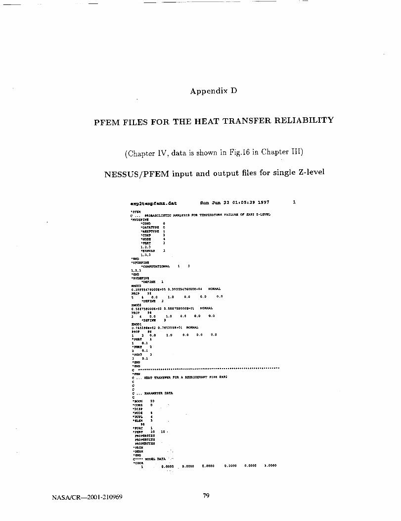
Appendix D
PFEM FILES FOR THE HEAT TRANSFER RELIABILITY
(Chapter IV, data is shown in Fig.16 in Chapter III)
NESSUS/PFEM input and output files for single Z-level
exp2tempfemz.dat Hun _ 22 01=05139 1997
C •.. PROBABIL_ST_C ANALYSZ0 FOR TEMPERATURE FAILURE Or EXp2 Z-LEVEL
• COND 0
• DA?&TYPZ 0
• _S P'i'Y PE 1
• CO_[p 2
•NOD_ 6
•PERT 3
1,2,3
• P,_3VAP, 3
1,2,3
*ZrOEF2_
• CONI_TTATIG_g_ l 3
2.2,3*1_'O
*KVOEl, nq
• DIIFINX 1I_OD3
0.3)5554?EO00E+O5 0. 3995547E000E*04 NOP_L_,
PROP 98
5 6 O O 1.0 0,0 0O O.0
• DErlN1E 2
]!_OD2
0.5|$755000_*03 0. 5007500001*01 NORMALPROP 98
3 4 0.0 1,0 0,0 0,0 0,0
• DOFI_E ]
_T,,[OB 1
0.TIS]SEE*02 0.?BS398E*01 NOlUt_LPROP Se
1 2 O,O 1,0 0,0 0,0 0,0
• ?E_T 11 0.1
°nX7 2
Z 0.1
• P_? 3
3 0.1
*I_SD*ID/D
C I)et •*moo*cote••••'elm me• ere'" me" e'e'oes se" e'*t •to e_'*) e''e ••e)tsee). e*. •
*m
C .,,
c
c
c
C .,.
c
*c_fs
*DISP*NC*DE &
*_UPL 4
*mJmM $
%8
*FORC 1*PERT 10
PROPERTIES
p_.OPEXT][t'S
PROPERTIES
*PRZH
*0EAM
C*'** MOD_L
*CO_K
NEAT TRANSFER FOR A REGEIGERANT PIPE EXP2
I*AIaJ_E'TI_q. DAT&
2O
0
DATA _ .-
0,0000 0,0000 0,0000 0,0000 0,0000 1.0000
NASA/CR--2001-210969 79

2 0.0000 10.0000 0.0000 0.0000 0.0000 1,0000
3 0.0000 10.0000 0.0000 0,0000 0.0000 1.0000
4 0,0000 20.0000 0.0000 0.0000 0.0000 1.0000
5 0.0000 20.0000 0.0000 0.0000 0.0000 1.0000
6 0.0000 30.0000 0.0000 0.0000 0.0000 1.0000
*ELEX 98
a 3 d
3 s 6
. D,,.Ip_3 2
s 4
"BOUN
6 1 0,0000
6 3 0.0000
1 1 0,0000
1 2 70.0000
1 3 0.00001 t 0.0000
1 S 0.0000
1 6 0,0000
1.0000 1.0000
*ITF, RA 1 340 0.0500
*PROP 90
1 2 1.0000 78,5390 0.3000 0.0000 2.SE-4
3 4 1.0000 S8.0758 0.3000 0.0000 2.32°4
5 6 1.0000 39955,4?6 0,3000 0.0000 2,5E-4
*PORC6 2 -241.66
"PRIN
TOT& NODE
*FPX
RI_RZG]Lq)..*_ PZPE I_£LZAB_LX'["Y WITH _-LE'V_,(T • S*FI
*R_ 3
*D&?I_'I_$ 4
* P_Itr_P'? 0
*_
*Z_ 1
5.00000
*1_10
exl)2tempfe_nz.o_tt; _ .a'run 22 01:06s_.6 '199"7
A0 ZS _E CONSTN4"I' TERN
AI. A2o .... AN JUSt THE DI_SlrGN SENSXT][V][?ZES
Xl, X2° ,.. , 3OI JU*.! THE IU_DOH VARYJ_llL_S
TAYLOR 81UtZltS COIL77ZCZlD/TS PANDOH I_XFANSZON NON(. D_SIGN
A ¢0111_S. VAM,'R VARZABbR POZN_ [NPP) SID/$_T_VZTY
..................................................................0 -0,?37506E+02
1 0.151374Z-OS 1 0.399555£*05 0.841409E-03
2 0.697150E*00 2 0.588758S*02 0.$?1068E*00
3 0.391765K÷00 3 0.785398E*02 0.428090E*00
PE:_PO_ZNO PROIU_ZLZSTXC J_/ALYgZS H_TH rP_
CDP R_.SUI, TSZ PROBABZLZI_Y ZT_R. NO.
0.50000000_÷01 0.13402715_*0t 0.90992140E÷00 0
NASA/CR--2001-210969 80

NESSUS/PFEM input and output files for CDF
eXlP2tezn_fem._rat 'l'hu Ap:c 6 17t14:48 1995
.pFI_
C . •. PROKkBZLZSTZC {CDP) AHAI,YSZ8 FOR ?_¢PEP._T_£ FA_LU!tJ; OF EXP2"HVDZP][_
*COND 0
*DATATYpE 0
"PJ_PYYPE 1
*COWP 2
eNODR 6
"PE_T 3
_.2,3
, PANVAR 3
1,2,3'_ND
"ZFDEFI_J
*COMPS;TAT IDEAL 1 3
1.2.]
"Oro
. RVOBF'INE
"DZFIIfl_ 1
ID,lOO3
n. 399554TI;000E*05 0. 399554"/&000E+OS _'DI_U_L
PROP 98
5 f 0.0 1.0 0.0 0.0 0.0"DEFZKE 2
O',OD_
0.SSS?SB000E*02 0._Sa758000E*01 NORMAL
PROP 98
3 4 0.0 1.0 0.0 0.0 0.0
*DE?INE 3104001
0.78539EE+0_ 0.78539|E_01 NOFU4AL
PROP 98
2 2 0.0 1.0 0.0 0.0 0.0
*PERT 11 0.1
*PERT 2
2 0.1
°P_T 3
3 0.i
*END*E_D
C ot*o,.**,.,eet.o,,olo*t,,o,o**.**,*,,oo,o.,**,***,**,,**..**.**.,.o._o
oPEX
C ... _T TRANSFER POR A REGRIGERANT PZPE EXp2
C
C
C
C ... PAJUtH_r_ DATA
C
*CONS 0
*DZSP
*NODE 6_D_/PL 4
*ELE_ 3
98
*FORC 1
"PRI_T I0 10 "
PROPERTIES
PROPERTIES
PROPERTIES
*PRIN
*SEN4
C "°** ;fODEL DATA
"COOR1 0.0000 0.0000 0.0000 O.0O00 0.0000 1.0000
NASA/CR--2001-210969 81

2 0.0000 10,0000 0,0000
3 0.0000 10.0000 0.0000
4 0.0000 20.0000 O.00OO
5 0.0000 20,0000 0.00006 0.0000 30.0000 0,0000
*E_IDS _8
3 3 43 5 6
°DUPL
3 2
S 4"DOUN
6 1 0.0000
6 3 0.00001 1 0.O000
1 2 10.0000
1 3 0.0000
1 4 0,0000
1 5 0.0000
1 6 o.ooo0
"BEAM I
1 6 1.0000 1.OO00
*ITE_ 1 3O.OSO0
*PROP 98
1 2 1.0000 78.5398 0._000 0.0000 2.5_-4
4 1,0000 5Lt?Si 0.3000 0.0000 2,5R-4S 6 1.0000 399_5,476 0.3000 0.0000 2,5E-4
*FORC
$ 2 -_tI.6G
"PRIN
TOTA lODE
C *'*'''''''*****''*'*'*oo**,**,**,-******,,*,*,,,,*,,,,,,,,****,**oo,,*FPZ
HEAT £XCHAGER OF EXp2 WITH DATAS_T$*R%_Ut4 3
*DATASETS 4
"METHOD 1
' PHI h'TOI_ 0
*ANA.wrYpE 0
*E3._
0,0000 O.O00O 1.0000
0.0000 0.0000 1.0000
0.0000 0.0000 1.00000.0000 0.0000 1.0000
0.0000 0.0000 1,0000
exp2temZ)£em.out Mon May 19 22:40:36 1997
AO Is THE CON_IT;U_T TERM
AI, A2, ,.. , AN ARE THE DESIGN SENSITIVITIES
X1, X2, ... , X_ARE THE RANt)ON VARIABLES
TA_ SEklZS COCFFZCII_TS PAKOOK EXP/_S[OK NORM. DESIC_
A COJ_'Fg. VALUE V_IKEIbE POINT (HPP} SE_SrTIVITY
..................................................................
0 -0.73_506E+02
1 0.1513741-05 1 0.399555E*05 0.$41489_-03
2 O._971SSE*00 2 0,588758¢*02 0.571068E_00
] 0.391765E_00 3 0.TOS39$E+02 0.425090E_00
P£_'O_It_Q PROIAEILXSTZC ANALYSIS WITH FPZ
CDP RESULTS
Z U PROBABILITY ITER_ NO.-0,2_0390_2E_02 -O.SI000000E_0_ 0.170122311-06 0
°0.2290S911_÷02 -0.4L000000E*01 0.2066871_E-04 0
-0.1777S790_02 -0.31000000E*01 0,967_7122E-03 0
-0.1264|63_E÷02 -0.21000000E_01 0.I_854357E-01 0
-0.75101880E÷01 °0.II000000B_01 0,13566610E*00 0
0.27418135_÷01 0.90000000_00 0.115939_I£*00 0
0.?Q?I9648E*01 0.19000000|+01 0.$7128351E_00 0
0.13002116_*02 0.2_000000E+01 0._9B13412£+00 0
0.1mI322E?E*02 0.390000QOE*01 O,999951BSZ_00 0
0.23262411E*02 0.4_000000E*01 0.99995952E.00 0
NASA/CR--2001-210969 82

Appendix E
PFEM FILES FOR RELIABILITY OF FLUID FLOW
(Chapter IV, data is show in Pig.18 of Chapter III)
NESSUS/PFEM input and output files for a single Z-level
flotrpfemz,d&t: Sat Juzl 28 22:36z52 1997
,PF_
C .... PEO3ABILISTIC AHALY$1S FOR FLOW FAILURE
*MVD_INE
• COND 0
I DATATYPS 0
"RESPTYPE I
"COMP 2
•NODE 2
• PERT 2
1.2
• JU_;VA_ 2
1,2
on4D
"ZFDEFINE
"COMPUTATIONAL I 2
t,2
,l_;D
"RV_EF_NE
"DEFINE 1
E_OD
14.8%6 _.4896 NORMAL
F_OP 98
1 ._ 0,0 l.O O,O O.D O.O
°DEFINE 2
VELO
-350.0 _$_0 _R_LL
FORD
2 2 I*00
"p_RT I
1 0.1
• PE_T 2
2 0.1
*_ND
-E_D
C .,,,°1°,o,°.°*,t,1o°,.°,,°o.1,*o,,**, o,. o, ,o,.-*o, ,*,°,
"F_4
C ... FLOW IN A CONSTANT DIAMETER PZPE (wi_h A/L_0.11
C
C
C
C .,, pA_AHET£E DATA
C"BOtIN 20
"CONS 0
"DZSP
"NODE 2
9B
"FOEC I
"FZ_T 10 10
VELOCITY
FORCE
°PRI_
OBEAJ4
*G_D
C _o*" MODEL DATA
"CODE
I 0. 0000
2 O. 0000
"[L[2¢ 95
I I
°BO_ _ I 0. 0000
2 3 O,0000
1 ! 0. 0000
i 2 1838.?
I 3 0. O000
0.0000 O.O000 O.OOOO O.OOO0 t.O000
I0.000 O,O000 O.OOOO 0.0000 1.0000
NASA/CR--2001-210969 83

1 4 0.0000
1 5 0,0000
1 6 0.0000
*2EAM 1
1 2 1.0000
°ITZRA 1 2
40 0.0S00
°PROP 98
1 2 1.0000
,FORC
2 2 -350.0
"PAIN
1.0000
It.8960 0,3000 0.0000 2.5E-4
TOTA NODE
*END
CH**o''''o ***o'*o*,,,,,,,*,,*,, o.,.o,,,,,oo.,,o, o,,,,,,..o,,.o,
°FP!
FLOW FAILURE PRQE&BILITY WITH Z-LEVEL IP<IETT.4psl)
• RVNUM 2
• GFTJNCT ION |
°OATASET$ 3
IMETNOD 1
° PRINTOPI" 0
"AHALYTYPE 1
"END
° ZLE'_ I
1677.4
° _D
DESZGN $ENSITZVITIES
........................................................................
TAYLOR SERIES EXPANSiON OFT HE FORM
G = &0 + AI"XI * A2*X2 * ... + AN'X.N
WHERE:
A0 IS THE CONETAHTTEPJ4
A1. A2 ..... AN ARE THE DESIGN SENSITIVITIES
Xl, X2 ..... XN ARE THE RANDOM VARIABLES
..................................................................
TAYLOR SERIES COEFPICI[I_TS P_DOH EXPANS[OW NOR.*4. DESIGN
R COEFF5. VALUE VARIABLE POINT (NPP) SENSITIVITY
..................................................................
0 0.160374E+04
£1owpfemz.out Bat Jun 28 22137t13 1997
1 0.1STT3SE*02 1 0.148%60E*02 0, S000OOE*O0
2 0. 671321E*00 2 -0. )50000E+03 -0. 50000DE*00
PEP.FORMING PROBABILISTIC ANALYSIS WITH FPI
CDF RESULTS
Z U PROBABILITY ITER. NO.
0.167740DOE+04 0.221";4074E*01 0. 98670241E_00 0
NASA/CR--2001-210969 84

NESSUS/PFEM input and outpout files for CDF
£1owcdf.dat Sat Jun 28 22:45:21 1997
.... PROBABILZSTIC ANALYSES FOR FLOW FAILURE
oMVDEFINZ
*COND 0
"OATATTPE 0
IRESPTYPE 1
°COMP 2
*NODE
• PE_T 2
1,2
*RA_VAR 2
1,2
"END
"ZFDEFINE
*COMPUTAT ZO_IAL 1 2
1,2
"END
*R_/DEFINE
"DEFINE I
ZMOD
14.896 1.4896 NORMAL
PROP 98
1 2 0.0 1.0 0.0 O.0 0.0
*DEFINE 2
VELO
-350.0 35.0 NO R.I¢_
FORC
2 2 1,00
"PERT 1
1 0.1
"PERT 2
2 0.1
"END
CE_,o.o°o°o,°,,o.o,,o°°°oo.,,o,,,,°o,°,,o,**° .... *°o,,°,.,
oFI_I
C .., FLOW IN A CONSTANT DIAMETER PIPE (with AIL=0.1)
C
C
C ,.. pARAMETER DATA
C
"BOUN 20
*CONS 0
"DISP
tNOD£ 2
"F.Zdi_ 1
98
• ?ORC 1
"PE._T 10 7.0
VEI,_C ITY
FORCE
ePXIN
"BEAN
"END
C it'_ MODEL DATA
°COOE
1 0.0000 0.0000 0.0000 0.0000 0.0000 1.0000
2 0. 0000 10,000 0,0000 0,0000 0,0000 1. 0000
"ELIM 9B
1 1 2
"IK_ 1 0.0000
2 3 O. 0000
1 1 0. 0000
1 2 1838.?
1 3 0.0000
NASAJCR--2001-210969 85

t. 4 0.0000
1 S 0.0000
1 6 0.0000
• SEAM 1
1 2 1.00O0 I 0000
° ITERA I 2
40 O.0S00
• PROP 98
1 2 1.0000 14.896 0.3000 0.0000 2.5£-4
• I?OEC
2 2 -350.0
"PRIN
TOTA NODE
"END
C,,to.tt,t°,,o.,*,,*,,0t o***o,0,,.*,°,,,,_.*,o,o,,*,o,oo,-*''***
°pp!
FLOW FAILURE PROBABILITY WITM A SERIES Z-LEVELS
°EVNUM 2
• GFI_IC_|ON 1
° DATA_ ETS 3
°METHOD l
°_RIM'_OF_ 0
"ARALYTYPE 0
.DrD
DESIGN SEN S I T I V t T _ E S
........................................................................
TAYLOR SERIES EXPANSION OF THE FORM
G • AO • AI°X_ • A2"X2 _ . .. * AN °XN
_HERE :
R0 IS THE CONSTANT TERN
At. A2, .... AN ARE THE DESIGN S_$4SIT_V_T_ES
X_, X2, XN _E THE RANDOH VARIABLES
TAYLOR SERIES COEFFZCI_TS
A C0SFFS. VAE_JE
..........................
0 0.160374E*04
RAHDO_4 EXPANSION HORn4. DESIGN
VRRI_LE POKNT iMPP) S_SITIVITY
........................................
flowcdf,out Sat Gun 28 22:46:36 1997 3
1 0.157735E+02 I O. 1489t;OE+02 0,50GOOOE*00
2 O. E?I32_E*00 2 -0. 350000E÷03 -0. SO0000E÷00
PERIrORMING EROBABILISTIC A/4ALYSI$ WITH FPZ
CDE RESULTS
Z U
0.1434$1_6S*04 -0.SI000000E_01
0.14(?S)ESE*0t -0.41000000E*01
0.1500_$64S+04 -O.]IO00000E*01
0.15)39763_*04 -0.21000000E+01
0.15571)61E*04 -0.11000000E*01
0.16)36359E'04 0.90000000E*00
0.166115581,04 0.1_000000E_G1
0.170007S6g_04 0.2|000000E_01
O._3S2955g_Ot 0.3_000000E*01
0.17665154E_04 0.49000000E*01
PROEABILITY ITER. NO.
0.17012231E-0E 0
0.20665716B-04 0
0.96767122E-03 0
0.17|6435_E-01 0
0.13556610E*00 0
0.015_39_1E*00 0
0.97120351E*00 0
0.99513412E_00 0
0.99_99%52E*00 0
NASA/CR--2001-210969 86

Appendix F
GFUN.DAT AND GFUN.MOV FILES OF IMPOSITIONS
(Chapter IV, data is show in Fig.16 of Chapter III)
NESSUS/PFEM input gfun.dat and output gfun.mov files
gf_.d&t 'l"ue O'ul I 15:39:34 1997 1
cPFEM*.. PRDBABZLISTIC A_JU, YSZS FOR STRUC_J_ _LZ_ILITY
• M'd'JD_'F INE
"COND 0
*DATATYPE 0
*RESPTYPR 3
• COMp 3
*NODE 44
°PERT 2
1,2
* RANVAR 2
1,2
*END
•ZFDEFINE
*COMPUTATIONAL I 2
1,2
*_qD
° RVDEFINI_
*DERZNE 1
EMOO
0. I700000E*O§ 0.1700000E÷07 NORMAL
PROP 153
1 SE 0.0 1.0 0.0 0.0 0.0
*DEPZNE. 2
ALFA
0.9500000R-05 0.1900000E-05 NORMAL
PROP 153
1 50 0.0 0.0 0,0 1,0 0.0
• POT 1
1 0.1
*PERT 2
2 0.1
C •o•**_* ,** I ,•***•*****•**o* ***o**o*,o•*, o*****,*,****** o****,*o•**•***
C *..REFRIGERANT PIPE U_DER INSIDE PRESURE
C
C
C
C ... PARAMETER DATA
CCONS 0
*DISP
*NODE 58
°ELEH 28
153
*BOUN 20
*PRESSURE
*T_PEKATURE
*LOUB 2 1 3 1
• PERT 10 10
PROPERTY
PROPERTY
*PR_N
° END
C °°** MODEL DATA
*CO_R
1 -5.000 0.95
2 -4.500 0.95
3 -4.000 0.95
4 -3.900 0.95
9 -3.000 0.%5
6 -2.700 0.95
7 -2.400 0.95
8 -2.100 0.95
9 -1.000 0.95
10 -1.500 0.95
12 -1.200 0.95
12 -0.900 0,95
13 -0.600 0.95
14 -0.300 0,99
19 0.000 0.95
16 0.300 0.9_
17 0.600 0.95
18 0.900 0,95
19 1.200 0.95
20 1.500 0.95
21 1.800 0195
22 2.100 0,95
21 2.400 0.95
24 2.?00 0.99
25 3,000 0.95
26 I.$00 0,95
27 4.000 0.95
28 4.500 0.99
2% 5.000 0.95
30 -$.000 0.665
31 -4,500 0.665
3E -4.000 0.665
33 -3.500 0.665
34 -3.000 0.665
35 -2.700 0.669
36 -2.400 0.665
37 -_.100 0.$65
18 -I.800 0,665
39 -i.500 0.665
60 -1.200 0.665
41 -0.900 0.665
42 -0.600 0.669
43 -0.300 0.665
44 0.00O 0.665
45 0.300 0.669
46 0.600 0,665
47 0,900 0.665
48 1.200 0.665
49 1.500 0.665
50 1.600 0.665
51 2.100 0,665
52 2.400 0.665
53 2.700 0.665
54 3,000 0.669
55 3.500 0.665
56 4.000 0.665
57 4,500 0.665
58 $.000 0_665
*ELEM 151
1 1 30 31 2
2 2 31 32 3
3 3 12 33 4
4 4 33 34 5
5 5 34 35 6
6 0 35 36 7
7 ? 36 37 0
8 8 37 38 9
9 9 38 39 10
10 lO 39 60 _l
11 11 40 41 12
12 12 41 42 13
13 13 42 43 14
14 14 43 44 15
15 15 44 45 16
16 16 45 46 17
17 17 46 47 16
NASA/CR--2001-210969 87

19 19 48 4g 2020 20 4g SO 21
21 21 SO 51 22
22 22 SI 52 23
23 23 $2 $3 24
2t 24 S3 $4 25
2S 25 S4 55 2626 26 55 56 2?
27 2_ $6 ST 2&
28 28 97 58 29
*PRBSStTRE
'JL_e _T_I _. 15t39t34 1997 2
30 58 3300.0
*TJ_PERATUIRE
1 2g 4.06
30 50 4.0
"BOU_
15 1 0.044 7. Q .0
• ZTEP.A 1 2
40 0.0500
"PROP 1S3
1 58 0.1000M:_0_ 0.1700E÷Cl8 0.3tO 0. g5001_°05 0.316_ 6.01_06
°PRZN
STRE NODI_
C I, e°,, ,,**,**°,,,,°**, °*,** ,°*°o,_,t***°,°_o o*°*o I**o* • o*_*ot*t* J**,*
oFP_
lIE.AT EXC'P.AGI_R OF RXP2 t,_'Jr_4 D,t,T,_.qETS
* P.V_U1_ 2°_Ir',_CTZOW 1
* DkT_rl's 3
, I_THOD 1
* yRIN'i_PT 0
o ,_'_ALTYP E 1
°ID_* ZLRVU.S I
0. &O00OOE,_04
° ID,_D
'JL'ue o"ul 1 15s28s37 1997 1
COHDI'f IOH | NOD1E CC44_HID4T l.kTl_.................................
ZI_CR 0 44 3 |
Z N£DZJUq. KEAN. STD. DEV.
0.454S371_04 0.654937B÷04 0.212524Et03
mERQF PROIL_BZL_TY _ 1
LVI,° Z0, _, _ROB. - 1 0.800000E*04 6.|2S?0 1.000000000
DES_G_ IP3_'? CO_IU3., SIDTS_TIVTTY _CTOP, S, S'FD. DEV. _¢NgVJkLUESZO, PIRO|. - 0.800000E*04 1.000000000
IUtOD 0.S3_6_tE_0_ O.g_9_S_ °6._2t_33
ALFA 0.96tS2T$B-05 -0.OISO_? 0.10277S
B.*°°oo''*e****.._Ot°,.otoo*_oQtt.*
_'DF RJ_SULTS
Z U PROBAJiZLITY
0.80000000E_04 0.68256956K_01 0.100000002_01
ITEm. NO*
0
NASA/CRy2001-210969 88

g_u.tl. _ov 8u_ _ 29 03316t&5 1997 1
CONDITZON 0 NODE COHPONE3_T I,_.YER.................................
_N_R 0 44 3 1
Z HEO_J_, NEAN, STO. DEV,
0.6_8271E_0d O.G?8271E*04 0.212754E_03
_F.,_ OF pROfU_LZTY L_,rltZ_ 1
LVL. Z0, U. PROB. • 1 0.800000_+04 5,72159 _.99959999_
DESZGN I_ZBrF COORD., $_S_TZVZTY FACTORS, S'CD. DEV. _OM V_AHVAIA_$
_0. _ROB. * 0.800000E_04 0.999999995
_4OD 0.7274407E_09 0.99988_ -5.?2093?_bFA 0.9664020R-05 -0.015008 0.006326
CI:)Y RLS"UL,TS
Z U PROBABILITY ZTI_, NO.0.80000000E_04 0.S7215001X_01 0.999999_9E÷00 0
g fUll.tonY B"" O_m 29 03311t36 1997 1
CONDI'1"20N J NOD£ COHPON _1"1' [,AVER.................................
INCR 0 44 3 1
Z HEOIAH, HEAN, STO. OEV,
0.701604E*04 0.?0160(E*04 0.212994E÷03
NUI4B£R OF PROB&BILZTY L_'Vl_LS 1
LVL. _0, _, PROB. • 1 0.800000E÷04 4.61965 0.999990076
OESIGN POINt COORD.. SENSITIVITY FAC'I_I_, STD. DEV. FNOH _VA_/ES
Z0, PROB. = 0.800000R_04 0.9999_076_JOD 0.9187492_*_9 0.P_9886 -4.619132
_FA 0.9632282E-05 -0.015071 0.0_9622
*,*°o***t**,*,,**°***°*°o-°.,,.,**.
CDFP, ESU_TS
Z U PRO_,_ZLI_ I_l_. NO.
0_80000000E*04 0.46196471E+01 0.99999808E+00 0
_'f u._.. too'v" B_m _ 29 03s13t50 1997 1
CON'_ZT30N ! NOTRE COHFONEI_T L_YER
.................................
ZNCR 0 4t 3 1
Z MEDIA_. HEAN. $I_. DEV.
0.?48271E*04 0.740271E÷04 0.213454E÷03
NU_4_ER OF _ROBA_IL_Y L_'VE_S 1
LV_. Z0, U, PROB. - I 0.&00OOQE÷04 2.42343 0.$_231262_
D_S2ON PO_ COORD.. $_Z_ZVZTY F&C"I_RS, S1rO. DEV. F_ON _UO_Vk_J_$Z0, PROB. - 0.800000E_04 0._9231_$28
E_OD 0.12BS064E*08 0.9_9887 -2.423155
AL_& 0.956_244E-05 -0.01S030 0.036444
C'_F RE_ULT_
U IPROBJ_I LZ TY 3TI_R. NO.
0. 80000000E÷04 0. 242342_2E÷01 0,9_232263R+00 0
NASA/CR--2001-210969 89

g£uzl.mov '1%re ,-ul 1 15:39z56 199"I
CDN_ZTZOH | NODE COHFON_T LAYER.................................
XNCR 0 44 3 1
Z HEOZAN. NEA.K, S'L_. DE_'.
0. ?71&041'J'04 0.7'716041!_,04 0,2134942",03
N',_'_n OF' PROEADr_ZTY ._I_S 1
_.VL, 7.0, _,1, MtOB. = 1 0.8000002*"04 1.32480 0°908043123
DESZGN FOIN'L' COOPdO., SID_SI'_IVITY FACTORS. $TD. DIW. FRON _ VA.T_UIE8'_O. /'_O]b. • 0. 80000Q'E_04 0.808043163
1_400 0,1474125'1_'08 0. 9941887 -1.328451
_k 0,9_,3_922a-0,S -0.0_.S021 0.01_'961.
****°*°°********.******°.**°*......
CDr _UT,?S
Z U IJlloaJuJzbz'rY I_'1_. NO.
0.SO0OOO00E*04 0.1324B012g*01 0.90804318Z_00 0
g£_,lm,_v 'l_e _1 1 15:36:47 1997 1
CON'DZTION | NODE OONI_H_ L.A'_/_.................................
IN_ 0 44 3 1
Z KEOZJ_. HEAN, STD. DEV.
0.794_38Z*04 0.794938B*04 0.2239242-03
KU_BF_R OF' PROIULBZLITY _ 1
LVL° Z0, U. PROB. - 1 0,800000_*04 0.83464 0,5935319g0
DUlG_ PO_]_T COORD., S_SITI_'fTY FACTORS, SI"D. DEV. FROH HEANVIJ.UF.S
Z0, PROB. - 0.8000008*04 0.$93531990
_/00 0,I_S_7784.0| 0,99988| -0.236814ALFA 0.92047282°05 °0.014959 0,003540
***,.*********.**.°,,,......,.*****
CDF" RE._T.?$
_ ]FROBJ_ZLZ'I_t ZTF.X NO.O.SO000000N+O4 0.236640192*00 0.593531992÷00
gf_u:L,mOV 'l_e _1 1 16417:30 1997 1
CONOZ*_ZON 0 NODE COHPOt;]D_ l._Y_lk.... ; ............................
ZNCR 0 48 3 1
Z )_DZAN, NFJ_N, _JFO. 91¢V.
0.78_808R+04 O,_99_Ot_tOt 0.8139$I_03
IqUHNI_R OF' PROIIAI_LZ'I'Y _ 3
LVI.., Z0. _, I/'IO_. - I 0.8000002*0_ O.0L_4_ 0.80737758?DI'_II_N F'OINT COOKD., SN_TIVZTYF',EC'_"OI_, _l'O. DIL'V. FROH NEANV_
_0, I_.GB. - 0_O00Q0_*04 0.507377527
_OD 0.I_8$4Z*08 0.899887 -0.0104_
/U,_& 0.$S002272-05 -O.0_SO03 0.00027?
******....**.°***.*,_***°...°*°**..
COP P.E3U_TS
U EROaJ_BZ_ZTY Z?_. NO.
0,40OO000OE*O4 8.144_37382-01 8.587377872+00 O
NASA/CR--2001-210969 90

Appendix G
DATA AND OUTPUT FILES FOR CALCULATION OF UNION
PROBABILITY
(Chapter IV)
tem_.dat T_e JILl 1 16:23:17 1997 1
7, 2, 1
I, 17000000.0,1700000.0
2, 0.0000095,0.0000019
I, 6.825696
2, 5.721588
3, 4.619647
4, 2.423429
5, 1.328801
6, 0.236641
7, 0.018497
i, 6.825696 0.999887
2, 5.721588 0.999886
3, 4.619647 0.999886
4, 2.423429 0.999887
5, 1.328801 0,999887
6, 0.236641 0.999888
7, 0.018497 0.999887
-0.015057
-0.015088
-0.015071
-0.015038
-0.015021
-0.014959
-0.015003
Lower bound = 0.4926211
Upper bound = 0.4926211
NASA/CR--2001-210969 91


BIBLIOGRAPHY
[11Mahadevan, S., Mehta, S., Tryon, R. G. and Cruse, T. A.,"System Reliability
Design Analysis of Propulsion Structures", Presented at the International Gas
Turbine and Aeroengine Congress and Exposition, Cincinnati, Ohio, May, 1993.
[2] Ang, A. H-S. and Tang, W. H.,"Probability Concepts in Engineering Planning
and Design, Vol.I- Basic Principles", John Wiley & Sons, Inc., 1975.
[3] Ang, A. H-S. and Tang, W. H.,"Probability Concepts in Engineering Planning
and Design, Vol.II- Decision, Risk, and Reliability", John Wiley & Sons, Inc.,
1984.
[4] Pages, A. and Gondran, M., "System Reliability: Evaluation and Prediction in
Engineering", Springer - Verlag, 1986.
[5] Tung, A. T. Y. and Kiremidjian, A. S., "Application of System Reliability The-
ory in the Seismic Analysis of Structures", Earthquake Spectra, Vol.8, No.3,
1992.
[6] Incropera, F. P. and DeWitt, D. P., "Introduction to Heat Transfer, 2nd ed.",
John Wiley & Sons, Inc., 1990.
[7] Thomas, L. C., "Heat Transfer", Prentice-Hall, Inc., 1992.
[8] Logan, D. L., "A First Course in the Finite Element Method", PWS Publishers,
1986.
[9] Kraus, A. D. and Bar-Cohen, A., "Thermal Analysis and Control of Electronic
Equipment", Hemisphere Publishing Corporation, 1983.
[10] Janna, W. S., "Introduction to Fluid Mechanics", PWS Publishers, 1983.
[11] Southwest Research Institute, "NESSUS Reference Manual, Version 1.0", July,
1991.
[12] Southwest Research Institute, "A Short Course on Probabilistic Structural Anal-
ysis Methods & NESSUS Workshop, Vo,. II", 1990.
NASA/CR--2001-210969 93

[13] Dias, J. B., "The NESSUS Finite Element Code - User's Manual", Southwest
Research Institute, 1989.
NASA/CR--2001-210969 94


REPORT DOCUMENTATION PAGE FormApprovedOMB No. 0704-0188
Pubtic reporting burden for this collection of information is estimated to average 1 hour per response, including 1he time for rewewing instructions, searching existing data sources.
gathering and maintaining the data needed, and completing and reviewing the collection of information. Send comments regarding this burden estimate or any other aspect of this
collection of information, including suggestions for reducing this burden, to Washington Headquarters Services, Directorate for information Operations and Reports. 1215 Jefferson
Davis Highway, Suite 1204, Arlington. VA 22202-4302, and to the Office of Management and Budget, Paperwork Reduction Pro)ect (0704-0186L Washinglon, DC 20503.
1. AGENCY USE ONLY (Leave blank) 2. REPORT DATE J 3. REPORT TYPE AND DATES COVERED
June 2001 I Final Contractor Report4. TITLE AND SUBTITLE
Multidisciplinary System Reliability Analysis
6. AUTHOR(S)
Sankaran Mahadevan and Song Han
7. PERFORMING ORGANIZATION NAME(S) AND ADDRESS(ES)
Vanderbilt University
Civil and Environmental Engineering
2201 W. End Avenue
Nashville, Tennessee 37240-0001
9. SPONSORING/MONITORING AGENCY NAME(S) AND ADDRESS(ES)
National Aeronautics and Space Administration
Washington, DC 20546-0001
5. FUNDING NUMBERS
WU-705-30-11_)0
NAG3-1372
8. PERFORMING ORGANIZATIONREPORT NUMBER
E-12823
10. SPONSORING/MONITORING
AGENCY REPORTNUMBER
NASA CR--2001-210969
11. SUPPLEMENTARY NOTES
Project Manager, Christos C. Chamis, Research and Technology Directorate, NASA Glenn Research Center.
organization code 5000, 216---433-3252.
12a. DISTRIBUTION/AVAILABILITY STATEMENT 12b. DISTRIBUTION CODE
Unclassified - Unlimited
Subject Category: 05 Distribution: Nonstandard
Available electronically at hffp://_ltrs._rc.nasa.gov/GLTRS
This publication is available from the NASA Center for AeroSpace Information. 301-621--0390.
13. ABSTRACT (Maximum 200 words)
The objective of this study is to develop a new methodology for estimating the reliability of engineering systems that
encompass multiple disciplines, The methodology is formulated in the context of the NESSUS probabilistic structural
analysis code, developed under the leadership of NASA Glenn Research Center. The NESSUS code has been success-
fully applied to the reliability estimation of a variety of structural engineering systems. This study examines whether the
features of NESSUS could be used to investigate the reliability of systems in other disciplines such as heat transfer, fluid
mechanics, electrical circuits etc., without considerable programming effort specific to each discipline. In this study, the
mechanical equivalence between system behavior models in different disciplines are investigated to achieve this objec-
tive. A new methodology is presented for the analysis of heat transfer, fluid flow, and electrical circuit problems using the
structural analysis routines within NESSUS, by utilizing the equivalence between the computational quantities in
different disciplines. This technique is integrated with the fast probability integration and system reliability techniques
within the NESSUS code, to successfully compute the system reliability of multidisciplinary systems. Traditional as well
as progressive failure analysis methods for system reliability estimation are demonstrated, through a numerical example
of a heat exchanger system involving failure modes in structural, heat transfer and fluid flow disciplines.
14. SUBJECT TERMS
Probabilistic analysis code: System reliability analysis; System reliability computation;
Tensile stress: Yield strength; Structure analysis; Thermal-structural fluid system
' 17. SECURITY CLASSIFICATION :18. SECURITY CLASSIFICATION 19. SECURITY CLASSIFICATIONOF REPORT OF THIS PAGE OF ABSTRACT
Unclassified Unclassified Unclassified
15. NUMBER OF PAGES
10516. PRICE CODE
20. LIMITATION OF ABSTRACT
NSN 7540-01-280-5500 Standard Form 298 (Rev. 2-89)
Prescribed by ANSI Std, Z39-18
298-102

