multi phase computational fluid dynamics modeling...

IIUUSSTT IInntteerrnnaattiioonnaall JJoouurrnnaall ooff EEnnggiinneeeerriinngg SScciieennccee,, VVooll.. 1199,, NNoo..55--11,, 22000088,, PPaaggee 7711--8811

MMUULLTTII PPHHAASSEE CCOOMMPPUUTTAATTIIOONNAALL FFLLUUIIDD DDYYNNAAMMIICCSS

MMOODDEELLIINNGG OOFF CCAAVVIITTAATTIINNGG FFLLOOWWSS OOVVEERR AAXXIISSYYMMMMEETTRRIICC HHEEAADD--FFOORRMMSS

NN.. MM.. NNoouurrii,, AA.. SShhiieenneejjaadd && AA.. EEssllaammddoooosstt

Abstract: In the present paper, partial cavitation over various head-forms was studied numerically to predict the shape of the cavity. Navier-Stokes equations in addition to an advection equation for vapor volume fraction were solved. Mass transfer between the phases was modeled by a sink term in vapor equation in the numerical analysis for different geometries in wide range of cavitation numbers. The re-entrant jet formation, which is the main cause for the cavitation cloud separation, was modeled very well with a modification of turbulent viscosity. In regions with higher vapor volume fractions (lower mixture densities) a modification of the k turbulence model was made by artificially reducing the turbulent viscosity of mixture. Computed shapes of cavities were found to be in good agreement with those of the reported experiments. Simulation results also compared well with those obtained from analytical relations.

Keywords: Cavitation, Turbulent flow; Axisymmetric head-form

1. Introduction1

When the pressure in a liquid flow falls below the particular saturation vapor pressure, the liquid evaporates. This phenomenon, called cavitation, has many applications in the industry, and is categorized by a dimensionless cavitation number 20.5vp p v

where vp is the vapor pressure, is the liquid

density, p

and v

are the main flow pressure and

velocity respectively. When a liquid flows over a solid body, as the fluid velocity increases (or cavitation number decreases) five different cavitation regimes can be observed: incipient-cavitation, shear-cavitation, cloud-cavitation, partial-cavitation and super-cavitation. The cavitation regime that occurs at low cavitation numbers (or high flow velocity) is called super-cavitation. The cavity closure is a critical region that is characterized by its unsteady and unstable behavior. In this region, liquid and vapor are highly mixed and

Paper first received March, 12. 2007 and in revised form Jan, 20. 2009. N.M. Nouri, Department of Mechanical Engineering, Iran University of Science and Technology, Narmak, Tehran, Iran, [email protected] A. Shienejad, Applied Hydrodynamics Laboratory, Department of Mechanical Engineering, Iran University of Science and Technology, Iran A. Eslamdoost, Applied Hydrodynamics Laboratory, Department of Mechanical Engineering, Iran University of Science and Technology, Tehran, Iran

experience a strong interaction of the cavity and the outer flow. Most of the erosion occurs at the vicinity of the closure region and is caused by the collapse of traveling small cavities. The vapor structures formed in the low pressure zones are transported downstream and collapse violently when they pass the higher pressure zone. In the presence of a multiphase flow, the turbulence modeling would be considered by separate models for each phase. The complexity of this approach leads major researchers to be careful the classical homogeneous turbulence formulation. Some researchers consider the idea based on the modification of classical two-equation turbulence modeling. Vaidyanathan and Senocak[1-2] proposed a non-equilibrium k based on the correction of the model coefficients to fit the experimental data based on optimization techniques. The difference between the computational and experimental results is used to judge the model fidelity. Coutier-Delgosha et al [3] and Reboud et al.[4] have introduced an artificial compressibility effect on the classical incompressible k modeling. The main idea is to avoid the high diffusivity of the numerical model caused due to the addition of the artificial viscosity t . Besides

cavitation, serious implications of turbulence modeling on cavitating flows were recently revealed by Wu et al. [5]. They reported that high viscosity of the original k model dampens cavitation instabilities.

id7308109 pdfMachine by Broadgun Software - a great PDF writer! - a great PDF creator! - http://www.pdfmachine.com http://www.broadgun.com

mailto:[email protected]

72 MMuullttii pphhaassee CCoommppuuttaattiioonnaall FFlluuiidd DDyynnaammiiccss MMooddeelliinngg ooff CCaavviittaattiinngg ��

Consequently, simulation of the phenomena such as periodic cavity inception and detachment requires alternate modeling approaches. Alternatively, Johansen et al.[6] have recently formulated a filter-based RANS turbulence model. The new model imposes a grid independent filter on the flow. While the imposed filter size prevents excessive dissipation of small-scale motions like the original RANS model, it allows development of flow scales corresponding in size with the grid resolution. Thus, the resultant behavior of the model can be tuned between the limits of RANS-type and a hybrid RANS-LES model. In this paper, in order to modeling the unsteady and shedding behavior of cavitation, two of the above-mentioned methodologies (Coutier-Delgosha et al.[3] and Reboud et al.[4]) as well as the methodology from Johansen et al.[6] were performed. The re-entrant jet formation is formed very well with these modifications.

2. Governing Equations The vapor-liquid flow described by a single-fluid

model is treated as a homogeneous bubble-liquid mixture, so only one set of equations is needed to simulate cavitating flows:

0m m jj

ut x

( ) ( )

(1)

( ) ( )

2( )( )

3

m i m i j

j

ji kt ij

i j j i k

u u ut x

uu up

x x x x x

(2)

The Equation(1) is continuity and the Equation(2) is momentum equation. In these equations, the constitutive relations for the density, dynamic viscosity and turbulent viscosity of mixture are as following:

(1 )m L L V L (3)

(1 )L L L V (4)

2m

t

C k

(5)

The subscript L and V stand for the properties of pure liquid and pure vapor, which are supposed to be constant. Additionally, a transport equation for the vapor-mass fraction f is required. This transport

equation is:

( )

.( )mm i

ff u m m

t

(6)

In the Equation, m stands for the appropriate cavitation mass transfer sink term.

3. Turbulence Modeling For the system closure, the original k

turbulence model with wall function is utilized as follows:

( )( ) m jm tt m

j j k j

u kk kp

t x x x

(7)

2

1 2

( )( ) m jm

j

tt m

j j

u

t x

C p Ck k x x

(8)

The turbulence production, Reynolds stress tensor terms, and the Boussinesq eddy viscosity concept are defined as:

2

3

it ij

j

ij i j

ij jii j t

j i

up

x

u u

k uuu u

x x

(9)

The empirical coefficients originally proposed by Launder and Spalding [7] assuming local equilibrium between production and dissipation of turbulent kinetic energy are as follows:

1 21 44 1 92 1 3 1kC C

. ; . ; . ;

4. Turbulence Modifications

As mentioned before, because of the deficiency of the original k model in predicting shedding and unsteady behavior of cavitating flow, we must modify this turbulence model. This problem is due to non-adequate turbulent viscosity predicted in cavity regions. Three suggestions are proposed in the literature to modify this simulation method. The first suggestion is to use k turbulence modeling with compressibility effects� correction proposed by Wilcox

[8]. The second suggestion is to reduce turbulent viscosity in the cavity region using the following relation (from Coutier et al.[9]):

2

1; 1

n

m Vt V n

L V

KC n

(10)

This modification limits the turbulent kinetic energy in cavity region and consequently allows the formation of re-entrant jet and the cavitation cloud shedding (Dular et al. [10]). The third suggestion is to use detached eddy simulation (DES) form of k turbulence

N. M. Nouri, A. Shienejad & A. Eslamdoost 7733

model. In this form of k model, turbulent viscosity is calculated by the relation as follows:

2

3/2

.1,t m

kC min

k

(11)

where is smallest edge length of each numerical cell. This relation produces a hybrid RANS-LES behavior by allowing development of length scale, comparable to the numerical grid resolution [6]. The second suggestion is applied for the present study.

5. Cavitation Model To simulate cavitation, a liquid flow is initially

considered over the axisymmetric body. The value of liquid mass fraction f is then calculated at locations

where pressure drops below the vapor pressure. Numerical models of cavitation differ in mass transfer term m . Among the semi-analytical models, the most known are Singhal model [11], Merkle model [12], Owis and Nayfeh model [13] and Kunz model [14]. In present studies, we used the Singhal model. Source terms m

and m that are included in the transport

equation define vapor generation (liquid evaporation) and vapor condensation, respectively. Source terms are functions of local flow conditions (static pressure and velocity) and fluid properties (liquid and vapor phase densities, saturation pressure and liquid vapor surface tension). The source term are derived from the Rayleigh-Plesset equation, where high order terms and viscosity terms can be found in Singhal et al. [11]. They are given by:

2;

3V

prod L V v V

L

P Pkm C f p p

(12)

2(1 ) ;

3V

dest L V V g VL

P Pkm C f f p p

(13)

where f is vapor-mass fraction, k is turbulent kinetic

energy, and is surface tension. destC and prodC are

empirical constants to regulate mass transfer due to the evaporation and condensation respectively.

6. Numerical Method

An unstructured CFD code based on finite volume method is used for two- and three-dimensional calculations. The SIMPLE pressure based algorithm is applied to solve the fluid flow field. The diffusive flux is discretized using the second order central difference scheme, whereas the choice of discretization scheme for the convective flux often depends on the fluid flow conditions and also physical properties of fluid [15]. In the present study, the first order upwind (FOU) scheme is considered. In addition, a first order implicit

temporal discretization scheme is applied for transient calculations. For the present study, the transport equation based on cavitation models, which was described earlier, is implemented into the solver, and related modifications regarding the convection schemes and the pressure-based algorithm have been made for steady computations. To describe the underlying algorithm, the steady-state generic transport equation is adopted in vector form as:

u q

.( ) .( ) (14)

where is the generalized dependent variable, is

the diffusion coefficient, and the second term on the right hand side represents the source term for the transport quantity . This equation is transformed to

an integral form, suitable for finite volume discretization, using the divergence theorem:

( ).s V

u ndS q dV

(15)

Integration of this equation yields the following equation:

1 1 1 1 ,, , , , ,2 2 2 2

i ji j i j i j i j i jF F F F F b

(16)

where ,i jb is the integrated form of the source term and

,i jF represents the flux of at each control volume

face. ,i jF is composed to a convective and a diffusive

part as follows:

( ).conv diffcf cf cf cfF F F u nS

(17)

As mentioned before, the diffusive flux is discretized using the second order central difference scheme, whereas the choice of discretization scheme for the convective flux often depends on the fluid flow conditions and physical properties of fluid. In the FOU scheme, the value of the dependent variable is estimated using the upwind neighbor value. If one lets

1 2,i jF

be the first order flux at a control volume face,

determined through first order extrapolation of two immediate neighboring cells, then the scheme can simply be written as:

11 2 1 2 1 2

11 1 2 1 2

,0

,0

n ni i i i

n ni i i

f Max u

Max u

(18)

where u is the velocity component in the corresponding direction. Higher order spatial accuracy can be obtained by employing more grid points for extrapolation. However, it is known that second or


higher order accurate schemes for convection terms produce oscillations around discontinuities.

7. Pressure-Based Algorithm for Cavitating

Flows The pressure-based algorithm, when adapted for

steady-state computations, follows the spirit of the well established SIMPLE algorithm (Patankar [16], Patankar & Spalding [17]), with substantial extension to treat issues associated with curvilinear coordinates and multi-block interface. Basically, the momentum equations are discretized as:

( )u u uP P nb nb P d P PA u A u V P b

(19)

where u

pA

and unbA

are the coefficient of the center and

neighboring nodes, respectively, due to contributions from convection and diffusion terms. pV and u

pb

represent the volume of the cell and the source term, respectively. Note that the d operator is the discrete

form of the gradient operator. For the present study, there is no source term in the momentum equations; hence, it does not appear in the following formulation.

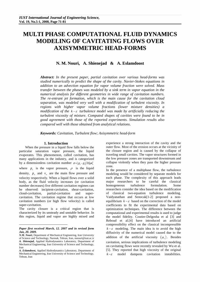
8. Boundary Condition

In this study inflow boundary was specified as a velocity inlet and outflow was specified as a constant pressure condition. At the inlet, the turbulent kinetic energy k is set to be equal to 5 23 10 inu . The value of

the specific dissipation rate is selected using the length scale equation (see [18]). On the wall, the boundary conditions are the impermeability and no-slip for the velocity, and the normal gradient of pressure is assumed to be zero. Wall functions based on the law of the wall are used as boundary conditions for the turbulence modeling. The applied boundary condition for axisymmetric and 3D configurations is sketched in Fif. (1) and Fig. (2). We used the axis boundary condition in the center-line of the computational domain where the normal gradient of the every variable in the flow domain is zero. Since the original k turbulence model together with the wall function is adopted, it is important to offer spatial resolutions consistent with the modeling requirement. This requires that the non-dimensional normal distance from

the wall y , a representation of the local Reynolds

number, should be in the log-law region. Once a cavity forms on the surface, the local Reynolds number decreases due to reduction in density, and the first grid point away from the wall may not be positioned in the log layer. This issue has important implications for both accuracy and convergence. We found that proper grid distribution is very important for satisfactory results and convergence of cavitating flow computations. For the present study, the non-

dimensional wall distance y was set to values

between 30 and 70, so that the logarithmic wall law can be applied. The grid is clustering near the wall boundary as shown in Fig. (3).

Fig. 1. Applied boundary condition for 2D

axisymmetric configuration.

Fig. 2. Applied boundary condition for 3D

computations

Fig. 3. Grid clustering near the solid wall

boundaries

9. Results and Discussion

9-1. Axisymmetric Numerical Simulation of Natural Cavitation: In �0through�0the numerical results for blunt body

head-form are plotted with the corresponding experimental results. As we can see, the calculation predicts the cavity length with high accuracy. The re-entrant jet will transport liquid phase into the cavitating regime at the end of the cavity. Visually, this will result in a closure of the cavity in a phase contour plot. It is also worth mentioning that the cavity length alone does not describe the flow. This can be seen clearly from the contour of constant void fraction plots shown in Fig. (4). In�0the plot of vapor volume fraction and selected streamlines was sketched, showing that while the cavitation number decreased the cavity length increased. The determination of the cavitation regimes was done by visual inspection of contour plots of the numerical solution. Rouse & McNown [�019] carried out a series of experiments wherein cavitations induced


by convex curvature aft of various axisymmetric fore bodies with cylindrical after bodies were investigated. At low cavitations numbers, these flows exhibit natural cavitation initiating near or just aft of the intersection between the fore-body and the cylindrical body.

Fig. 4. Volume fraction and selected stream lines for

cavitating flow over a blunt fore-body at 1.2

For each configuration, calculations were made between a range of cavitation numbers, including a single-phase case (large ). Surface static pressure calculations were taken along the cavitator and after-body. Snapshots were also taken from which approximate bubble size and shape were deduced. Several of the Rouse & McNown [19] configurations were analyzed. These included 0-caliber (blunt), 1/2-caliber (hemispherical), and conical (22.50-cone half-angle) cavitator shapes. The simulations were performed at Reynolds numbers greater than 100,000 based on maximum cavitator (after-body) diameter.

Fig. 5. Volume fraction and selected stream lines for

cavitating flow over fore-body at 0.3

Fig. (7) through Fig. (10) provide similar comparisons for hemispherical and conical fore-bodies. Specifically, �0and�0 Fig. (10) show comparisons between predicted and measured surface pressure distributions for these two configurations at a cavitation number of 0.3.

As we can see at the rear part of the cavitation zone, the flow was re-circulated and the liquid has been sucked to the cavitation region. In each case, a discrete bubble shape is observed, but the aft-end of the predicted bubble does not exhibit a smooth �ellipsoidal� closure. Indeed, due to local flow reversal

(reentrant jet), liquid is swept back underneath the vapor pocket. The pressure in this region retains nearly constant on free streamline liquid flow.

Fig. 6. Pressure coefficient distribution for blunt

fore-body at 0.3

Fig. 7. Volume fraction and selected streamlines for cavitating flow around a hemispherical fore-body at

0.3

Fig. 8. Pressure coefficient distribution for

hemispherical fore-body at 0.3


Fig. 9. Volume fraction and selected streamlines for cavitating flow around conical fore-body at 0.3

Fig. 10. Pressure coefficient distribution for conical

fore-body at 0.3

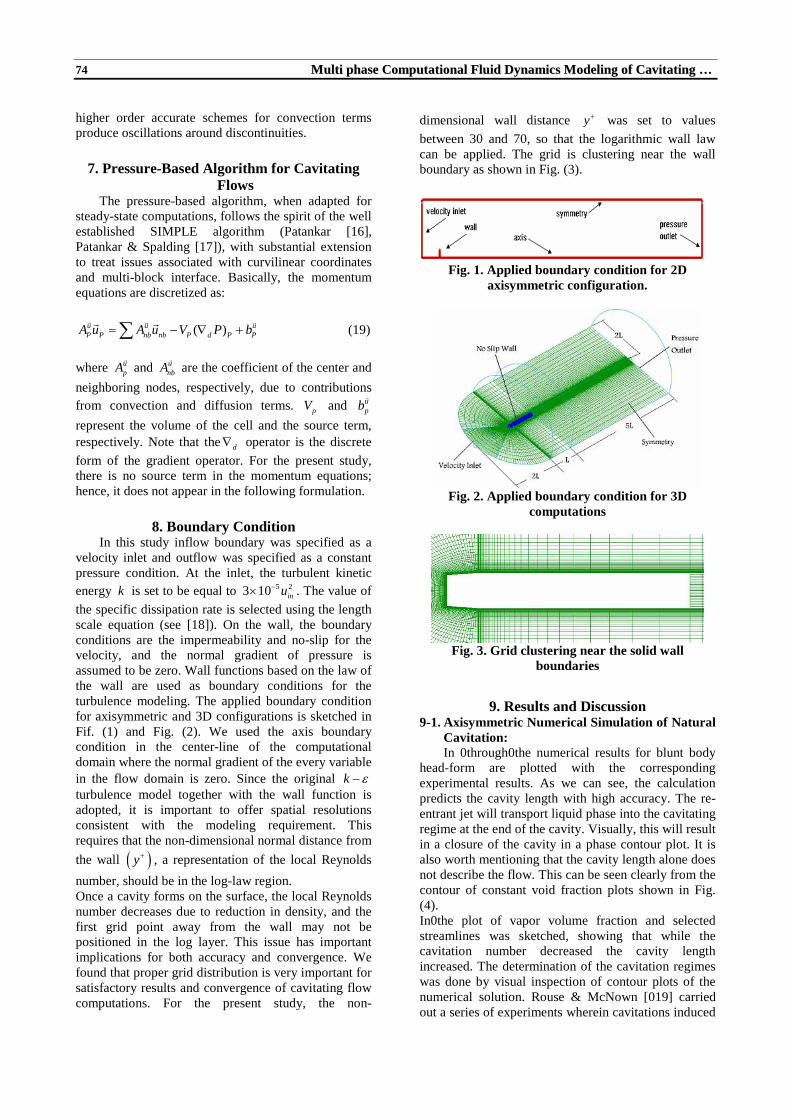
9-2. Cloud Cavitation Over Cylinder:

In this test case, we considered cavitation over a blunt cylinder and cylinder with hemispherical head at two cavitation numbers 0.3 26 /V m s

and

0.15 36 /V m s . In all the simulations, for

capturing the unsteady behavior of cloud cavitation and formation of re-entrant jet at the rear part of the cavity, turbulent viscosity was modified with the Reboud et al. [3-4] modification. The time evolution of cavity region at 0.3 is shown in Fig. (11). Cavitation starts and grows in vortices formed near the cylinder wall. The current simulations show that at

0.3 , cavity exhibits the periodic behavior of cloud cavitation. After the formation of a developed cavity (t=48ms), large vapor structures detach from the main cavity due to the unsteady movement of re-entrant jet; the cavity then grows again from the edge of the cylinder (t=57.5 ms). The detached region moves downstream and gradually disappears (t=62.5-65.5 ms). The newly developed cavity exhibits similar periodic behavior: inward movement of water jet, detachment of vapor structure and cavity growth (t=67.5-68.5 ms). It should be noted that the unsteady behavior of cloud cavitation results in a nonsymmetrical cavity shape, consequently more accurate simulation of this cavitation regime requires a three dimensional modeling [20].

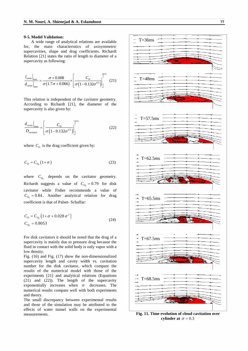
9-3. Three-Dimensional Partial Cavitation: In order to demonstrate the three-dimensional

capability of the code, a cavitation flow was simulated over a model of hemispherical fore-body configuration

at numerous angles of attack and 0.3 . The domain consisted of 8 blocks. Fig. (12) provides sample results for angles of attack of 0.0, 2.5, 5.0 and 7.5 degree. These plots include pressure contours on the plane of symmetry, sample streamlines and the cavitation bubble shape as identified with an isosurface of 0.99l .

Several interesting features are observed in the prediction. A recirculation zone aft of the bubble grows with the angle of attack. This diminishes the local pressure recovery associated with the bubble-induced blockage, and this in turn leads to a local collapse of the bubble on the top of the body. Indeed, at angle of attack the bubble is seen to have its great axial extend off the symmetry plane of the geometry. At this cavitation number, steady state solutions could be obtained.

9-4. Supercavitation Behind a Disk Cavitator:

In this section, we present the numerical simulation of cavitating flow over an axisymmetric body such as disk and cone with the head angle of 90, for which experimental and analytical results (such as Richardt Relation from Frane and Michel [21]) are available in the literature. For a cavitation number of 0.15 and a Reynolds

number of 6Re 8.6 10 40V m s , the steady

supercavity shape behind a disk is shown in �0 Fig. (13). For the case 0.15 , the contours of velocity and Cp are shown in�0 Fig. (14) and Fig. (15) Inside the

supercavity, there exists a core of reverse flow and vortices. The main concentration of reverse flow is located in the cavity center, identified by a pink color in�0 Fig. (14). with a maximum reverse flow velocity of about 30 m s . Outside this vortical core, the velocity is

relatively low, with an approximate absolute value of less than 10 m s .

Meanwhile, the range of velocity at the location of the re-entrant region is about 6 m s , which is about 17%

of the main flow velocity V

. As shown in�0 Fig. (15),

Cp contours vary from 1 at the stagnation point where

the flow impacts the disk to 0.15 inside the cavity. The contour of supercavity boundary is identified by 0.15 . It is observed that this value is equal to the negative value of the cavitation number which was expected because:

2 2 ;

0.5 0.5

inside thecavity :

v

v

P PP PCp

V V

P P Cp

(20)


9-5. Model Validation: A wide range of analytical relations are available

for, the main characteristics of axisymmetric supercavities, shape and drag coefficients. Richardt Relation [21] states the ratio of length to diameter of a supercavity as following:

0.5

max

0.5

max

0.008

1.7 0.066 1 0.132

cavity D

cavity

l C

d

(21)

This relation is independent of the cavitator geometry. According to Richardt [21], the diameter of the supercavity is also given by:

0.5

max

0.51 0.132

cavity D

cavitator

d C

D

(22)

where DC is the drag coefficient given by:

01D DC C (23)

where

0DC depends on the cavitator geometry.

Richardt suggests a value of 0

0.79DC for disk

cavitator while Fisher recommends a value of

00.84DC . Another analytical relation for drag

coefficient is that of Palset- Schaffar:

0

0

21 0.028

0.8053

D D

D

C C

C

(24)

For disk cavitators it should be noted that the drag of a supercavity is mainly due to pressure drag because the fluid in contact with the solid body is only vapor with a low density. Fig. (16) and Fig. (17) show the non-dimensionalized supercavity length and cavity width vs. cavitation number for the disk cavitator, which compare the results of the numerical model with those of the experiments [21] and analytical relations (Equations (21) and (22)). The length of the supercavity exponentially increases when decreases. The numerical results compare well with both experiments and theory. The small discrepancy between experimental results and those of the simulation may be attributed to the effects of water tunnel walls on the experimental measurements.

Fig. 11. Time evolution of cloud cavitation over

cylinder at 0.3

T=36ms

T=48ms

T=57.5ms

T=62.5ms

T=65.5ms

T=67.5ms

T=68.5ms


Fig. 12. Predicted three-dimensional flow fields with natural cavitation about hemispherical fore-body at

various angles of attack

9-6. Supercavitation Behind Cone Cavitator In another test case, the supercavity behind a cone

(with a head angle of 90 degree) was considered. For a cavitation number of 0.075 and a Reynolds

number of 7Re 8.9 10 51V m s , the result is

shown in Fig. (18). The ratio of cavity length to

diameter max maxcavity cavityl d is a function of and is

independent of cavitator geometry, as stated by Richardt Relation:

max

max

0.008

1.7 0.066cavity

cavity

l

d

(25)

The length and diameter of the supercavity increase as the head angle increases from 45 to 180 degree (a disk cavitator can be assumed as a cone with an angle of 180 degree).�0 Fig. (19) and Fig. (20) show the non-dimensionalized supercavity length and cavity width vs. cavitation number for the cone cavitator. The figures compare the results of the numerical model with those of the experiments (Frane and Michel [21]) and analytical relations (Equation (25)). It is seen that the numerical results compares well with both experiments and theory. The non-dimensional cavity width was compared just with experimental data of [21].

9-7. 3D Computation of Supercavitation: In this section, supercavitation at cavitation

number 0.02 on 3 for different cavitator with after body was modeled. Nondimensionalized supercavity length and width were considered as the main parameters. The geometry of three models is shown in�0 Fig. (21). Each model has a length of L with the circular section with diameter of D . The ratio of L D is 6 for three

models. Model 1 has a conical nose with angle of 60 degrees. Model 2 is a cut of conical nose at angle of 60 and model 3 has a hemisphere cavitator.

9-8. Results of 3D Supercavity Simulations: In Fig. (22) through�0 Fig. (24), the supercavity

pattern for three models are shown. In Fig. (25) and Fig. (26), the �cavity length/body diameter� and

maximum �cavity diameter/body diameter� for the

models 1, 2 and 3 at cavitation number 0.02 were compared with the results of Stinebring et al.[22]. (The experimental results were obtained at cavitation number 0.05). As mentioned before, by decreasing the cavitation number, the cavity length increased rapidly and this fact is observed as shown in�0 Fig. (25).

10. Conclusion In this paper, the transient and steady cavitating

flow over various cavitators was studied numerically. In order to simulate the unsteady behavior of cavity shedding and re-entrant flow field, the original kå

model was modified based on the modification which is proposed by Reboud et al [4]. The cavity shape compared very well with experimental data.

Fig. 13. Supercavity shape behind a disk at

0.15

0.0

2.5

5.0

7.0


Fig. 14. Contour of velocity at 0.15

Fig. 15. Pressure coefficient for disk cavitator at

0.15

Fig. 16. Supercavity length vs. cavitation number

for disk cavitator

Fig. 17. Nondimensional cavity width vs. cavitation

number for disk cavitator

Fig. 18. Supercavity shape behind cone cavitator at

0.075

Fig. 19. Supercavity length vs. cavitation number

for cone cavitator

Fig. 20. Nondimensional cavity width vs. cavitation

number for cone cavitator

Fig. 21. Geometry of three various cavitators with

after body

Fig. 22. Supercavity pattern at 0.02 for cone

cavitator with after body

Fig. 23. Supercavity pattern at 0.02 for cut off

cone cavitator with after body


Fig. 24. Supercavity pattern at 0.02 for

truncated hemispher cavitator with after body

Fig. 25. Supercavity length to body diameter for

models 1, 2 and 3

Fig. 26. Maximum cavity diameter to body diameter

for models 1, 2 and 3.

References [1] Vaidyanathan, R., Senocak, I., Wu, J., Shyy, W.,

Sensitivity Evaluation of a Transport-Based Turbulent Cavitation Model. Trans. of ASME, J. Fluids Eng. 125, 2003, pp. 447�458.

[2] Senocak, I., Computational Methodology for the Simulation Turbulent Cavitating Flows. PhD thesis, University of Florida, 2002.

[3] Coutier-Delgosha, O., Fortes-Patella, R., Reboud, J.L.,

Evaluation of the Turbulence Model Influence on the Numerical Simulations of Unsteady Cavitation. Trans. of ASME, J. Fluids Eng. 125, 2003, 38�45.

[4] Reboud, J.L., Stutz, B., Coutier-Delgosha, O., Two-Phase

Flow Structure of Cavitation: Experiment and Modeling of Unsteady Effects. Third Int. Symposium on Cavitation, Vol. 1, 1998, pp. 39�44.

[5] Wu, J., Utturkar, Y., Senocak, I., Shyy, W., Arakere, N., Impact of Turbulence and Compressibility Modeling on Three-Dimensional Cavitating Flow Computations, AIAA Paper 2003.

[6] Johansen, S., Wu, J., Shyy, W., Filter-based Unsteady

RANS Computations, Technical Report, University of Florida 2003.

[7] Launder, B.E., Spalding, D.B., The Numerical

Computation of Turbulent Flows, Comp. Meth. Appl. Mech Eng., Vol. 3, 1974, pp. 269-289.

[8] Wilcox, D.C., Turbulence Modeling for CFD, 2nd Edition

1998.

[9] Coutier-Delgosha, O., Fortes-Patella, R., Delannoy, Y.,

Numerical Simulation of Unsteady Behavior of Cavitating Flows, 2003, International Journal of Numerical Methods in Fluids.

[10] Dular, M., Bachert, R., Stoffel, B., Sirok, B., �Numerical

and Experimental Study of Cavitating Flow on 2D and 3D Hydrofoils,� Proceedings of the Fifth International Symposium on Cavitation, Osaka, Japan, 2003.

[11] Singhal, N.H., Athavale, A.K., Li, M., Jiang, Y.,

Mathematical Basis and Validation of the Full Cavitation Model, J. Fluids Eng., Vol. 124, 1-8, 2002.

[12] Merkle, C.L., Feng, J., Buelow, P.E.O., Computational

Modeling of the Dynamics of Sheet Cavitation, Proceeding of the 3rd International Symposium on Cavitation, (CAV98), Grenoble, France, 1998.

[13] Owis, F.M., Nayfeh, A.H., Numerical Simulation of 3-D

Incompressible, Multi-Phase Flows Over Cavitating Projectiles, European Journal of Mechanics B/Fluids, 23, 2004, 26, pp. 339-351.

[14] Kunz, R.F., Boger, D.A., Stinebring, D.R., Chyczewski,

T.S., Lindau, J.W., Gibeling, H.J. A Preconditioned Navier-Stokes Method for Two-Phase Flows with Application to Cavitation, Computers & Fluids, Vol. 29, 2000¸ pp. 849-875.

[15] Shyy, W., Computational Modeling for Fluid Flow and

Interfacial Transport, Elsevier, Amsterdam, The Netherlands, Revised Printing 1997.

[16] Patankar, S.V., Numerical Heat Transfer and Fluid

Flow, Hemisphere, Washington DC, 1980. [17] Patankar, S.V., Spalding, D.B., �A Calculation

Procedure for Heat, Mass and Momentum Transfer in Three Dimensional Parabolic Flows,� Int. J. Heat Mass Tran, 15, 1972, pp. 1787-1806.

[18] Ferziger, J.H., Peric´, M., Computational Methods for

Fluid Dynamics, Springer-Verlag, Berlin, 1996. [19] Rouse, H., McNown, J.S., Cavitation and Pressure

Distribution, Head Forms at Zero Angle of Yaw, Studies


in Engineering, Bulletin 32, State University of Iowa, 1948.

[20] Latt, K., Underwater express, DAEPA & ATO proposal

report, 2005. [21] Franc, J.P., Michel, J.M., Fundamentals of Cavitation,

Kluwer Academic Publisher, Netherlands, 2004. [22] Stinebring, D.R., Holl, J.W., "Water Tunnel Simulation

Study of the Later Stages of Water Entry of Axisymmetric Bodies: Phase II � Effect of the After Body on Steady State Ventilated Cavities," ARL Penn State Dec. 1979.

multi phase computational fluid dynamics modeling...

Documents