msr identity toolbox - microsoft.com · identity toolbox 1 msr identity toolbox: a matlab toolbox...

MSR Identity Toolbox Version 1.0

Seyed Omid Sadjadi

Malcolm Slaney

Larry Heck

Microsoft Research Technical Report

MSR-TR-2013-133

[email protected]

{mslaney,larry.heck}@microsoft.com

Identity Toolbox 1

MSR Identity Toolbox:

A MATLAB Toolbox for Speaker Recognition Research Version 1.0

Seyed Omid Sadjadi, Malcolm Slaney, and Larry Heck

Microsoft Research

[email protected], {mslaney,larry.heck}@microsoft.com

This report serves as a user manual for the tools available in the Microsoft Research (MSR) Identity

Toolbox. This toolbox contains a collection of MATLAB tools and routines that can be used for

research and development in speaker recognition. It provides researchers with a test bed for

developing new front-end and back-end techniques, allowing replicable evaluation of new

advancements. It will also help newcomers in the field by lowering the “barrier to entry”, enabling

them to quickly build baseline systems for their experiments. Although the focus of this toolbox

is on speaker recognition, it can also be used for other speech related applications such as language,

dialect and accent identification.

In recent years, the design of robust and effective speaker recognition algorithms has attracted

significant research effort from academic and commercial institutions. Speaker recognition has

evolved substantially over the past 40 years; from discrete vector quantization (VQ) based systems

to adapted Gaussian mixture model (GMM) solutions, and more recently to factor analysis based

Eigenvoice (i-vector) frameworks. The Identity Toolbox provides tools that implement both the

conventional GMM-UBM and state-of-the-art i-vector based speaker recognition strategies.

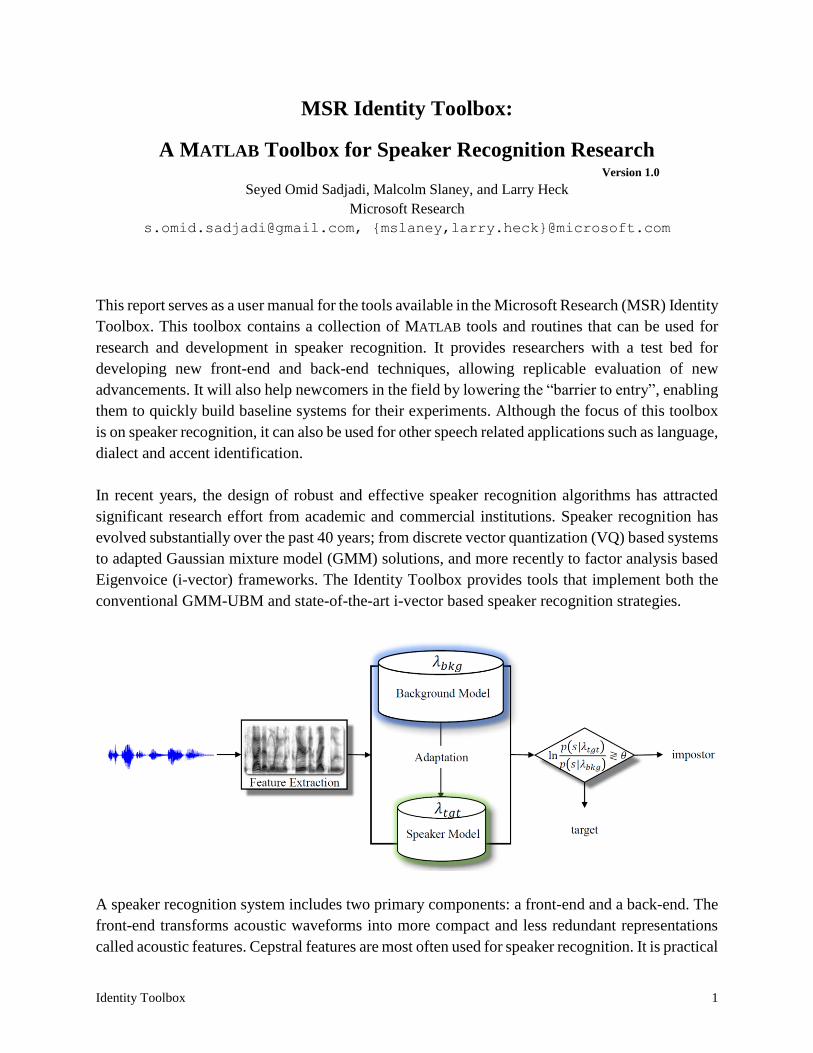
A speaker recognition system includes two primary components: a front-end and a back-end. The

front-end transforms acoustic waveforms into more compact and less redundant representations

called acoustic features. Cepstral features are most often used for speaker recognition. It is practical

2

to only retain the high signal-to-noise ratio (SNR) regions of the waveform, therefore there is also

a need for a speech activity detector (SAD) in the front-end. After dropping the low SNR frames,

acoustic features are further post-processed to remove the linear channel effects. Cepstral mean

and variance normalization (CMVN) is commonly used for the post-processing. The CMVN can

be applied globally over the entire recording or locally over a sliding window. Feature warping,

which is also applied over a sliding window, is another popular feature normalization technique

that has been successfully applied for speaker recognition. This toolbox provides support for these

normalization techniques, although no tool for feature extraction or SAD is provided. The Auditory

Toolbox (Malcolm Slaney) and VOICEBOX (Mike Brooks) which are both written in MATLAB

can be used for feature extraction and SAD purposes.

The main component of every speaker recognition system is the back-end where speakers are

modelled (enrolled) and verification trials are scored. The enrollment phase includes estimating a

model that represents (summarizes) the acoustic (and often phonetic) space of each speaker. This

is usually accomplished with the help of a statistical background model from which the speaker-

specific models are adapted. In the conventional GMM-UBM framework the universal background

model (UBM) is a Gaussian mixture model (GMM) that is trained on a pool of data (known as the

background or development data) from a large number of speakers. The speaker-specific models

are then adapted from the UBM using the maximum a posteriori (MAP) estimation. During the

evaluation phase, each test segment is scored either against all enrolled speaker models to

determine who is speaking (speaker identification), or against the background model and a given

speaker model to accept/reject an identity claim (speaker verification). On the other hand, in the

i-vector framework the speaker models are estimated through a procedure called Eigenvoice

adaptation. A total variability subspace is learned from the development set and is used to estimate

a low (and fixed) dimensional latent factor called the identity vector (i-vector) from adapted mean

supervectors (the term “i-vector” sometimes also refers to a vector of “intermediate” size, bigger

than the underlying cepstral feature vector but much smaller than the GMM supervector). Unlike

the GMM-UBM framework, which uses acoustic feature vectors to represent the test segments, in

the i-vector paradigm both the model and test segments are represented as i-vectors. The

dimensionality of the i-vectors are normally reduced through linear discriminant analysis (with

Fisher criterion) to annihilate the non-speaker related directions (e.g., the channel subspace),

thereby increasing the discrimination between speaker subspaces. Before modelling the

dimensionality reduced i-vectors via a generative factor analysis approach called the probabilistic

LDA (PLDA), they are mean and length normalized. In addition, a whitening transformation that

is learned from i-vectors in the development set is applied. Finally, a fast and linear strategy, which

computes the log-likelihood ratio (LLR) between same versus different speakers hypotheses,

scores the verification trials. The Identity toolbox provides tools for speaker recognition using both

the GMM-UBM and i-vector paradigms.

Identity Toolbox 3

This report does not provide a detailed description of each speaker recognition tool available. The

function descriptions include references to more detailed descriptions of corresponding

components. We have attempted to maintain consistency with the naming convention in the code

to follow the formulation and symbolization used in the literature. This will make it easier for the

users to compare the theory with the implementation and help them better understand the concept

behind each algorithm.

4

Usage

In order to better support interactive or batch usage, most of the tools in the Identity

Toolbox accept either floating point or string arguments. String arguments, either

for a file name or a numerical value, are useful when these tools are compiled and

called from a shell command line. This makes it easy to use the tools on machines

with limited memory (but enough disk space) as well as computer clusters (from a

terminal). In addition, the interactive tools can optionally write the output products

(models or matrices) to the disk if an output file name is specified.

This toolbox makes extensive use of parfor loops (as opposed to for loops) so that

parallel processing can speed up the computations. However, if the Distributed

Computing Toolbox is not installed, MATLAB automatically considers all parfor

loops as for loops and there is no need to modify the tools. MATLAB by default sets

the number of parallel workers to the number of physical CPU cores (not logical

threads!) available on a computer. At the time of writing this report, MATLAB

supports a maximum of 12 workers on a local machine.

The Identity toolbox has been tested on Windows 8 as well as Ubuntu Linux

computers running MATLAB R2013a. The toolbox is portable and is expected to

work on any machine that runs MATLAB.

Compilation

In case MATLAB is not installed or MATLAB license is not available (for instance on

a computer cluster), we provide standalone executables that can be used in

conjunction with the MATLAB Compiler Runtime (MCR). The MCR is a standalone

set of shared libraries that enables the execution of compiled MATLAB applications

or components on computers that do not have MATLAB installed. The MCR installer

can be obtained free of charge from the web address:

http://www.mathworks.com/products/compiler/mcr/

The binaries supplied with this version of the toolkit need version 8.1 (R2013a) of

the MCR.

The MCR installer is easy to use and provides users with an installation wizard.

Assuming that the MCR is installed, a MATLAB code can be compiled from either

the command window or a DOS/bash terminal as:

Identity Toolbox 5

mcc -m -R -singleCompThread -R -nodisplay -R -nojvm foo.m -I libs/ -o foo -d

bin/

for a standalone single-threaded executable. Single-threaded executables are useful

when running the tools on clusters that only allow a single CPU process per

scheduled job. To generate multithreaded executables (this is important when using

parfor) the mcc can be used as following:

mcc -m -R -nodisplay foo.m -I libs/ -o foo -d bin/

For more details on the “mcc” command see the MATLAB documentation.

6

Flow Charts

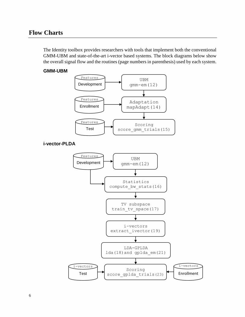
The Identity toolbox provides researchers with tools that implement both the conventional

GMM-UBM and state-of-the-art i-vector based systems. The block diagrams below show

the overall signal flow and the routines (page numbers in parenthesis) used by each system.

GMM-UBM

i-vector-PLDA

UBM

gmm-em(12)

Enrollment

Development

Adaptation

mapAdapt(14)

Test Scoring

score_gmm_trials(15)

UBM

gmm-em(12) Development

Scoring

score_gplda_trials(23)

Statistics

compute_bw_stats(16)

TV subspace

train_tv_space(17)

i-vectors

extract_ivector(19)

LDA-GPLDA

lda(18)and gplda_em(21)

Test Enrollment

i-vectors i-vectors

Features

Features

Features

Features

Identity Toolbox 7

cmvn

Purpose

Global cepstral mean and variance normalization (CMVN)

Synopsis

Fea = cmvn(fea, varnorm)

Description

This function implements global cepstral mean and variance normalization

(CMVN) on input feature matrix fea to remove the linear channel effects. The code

assumes that there is one observation per column. The CMVN should be applied

after dropping the low SNR frames.

The logical switch varnorm (false | true) is used to instruct the code to perform

variance normalization in addition to mean normalization.

Examples

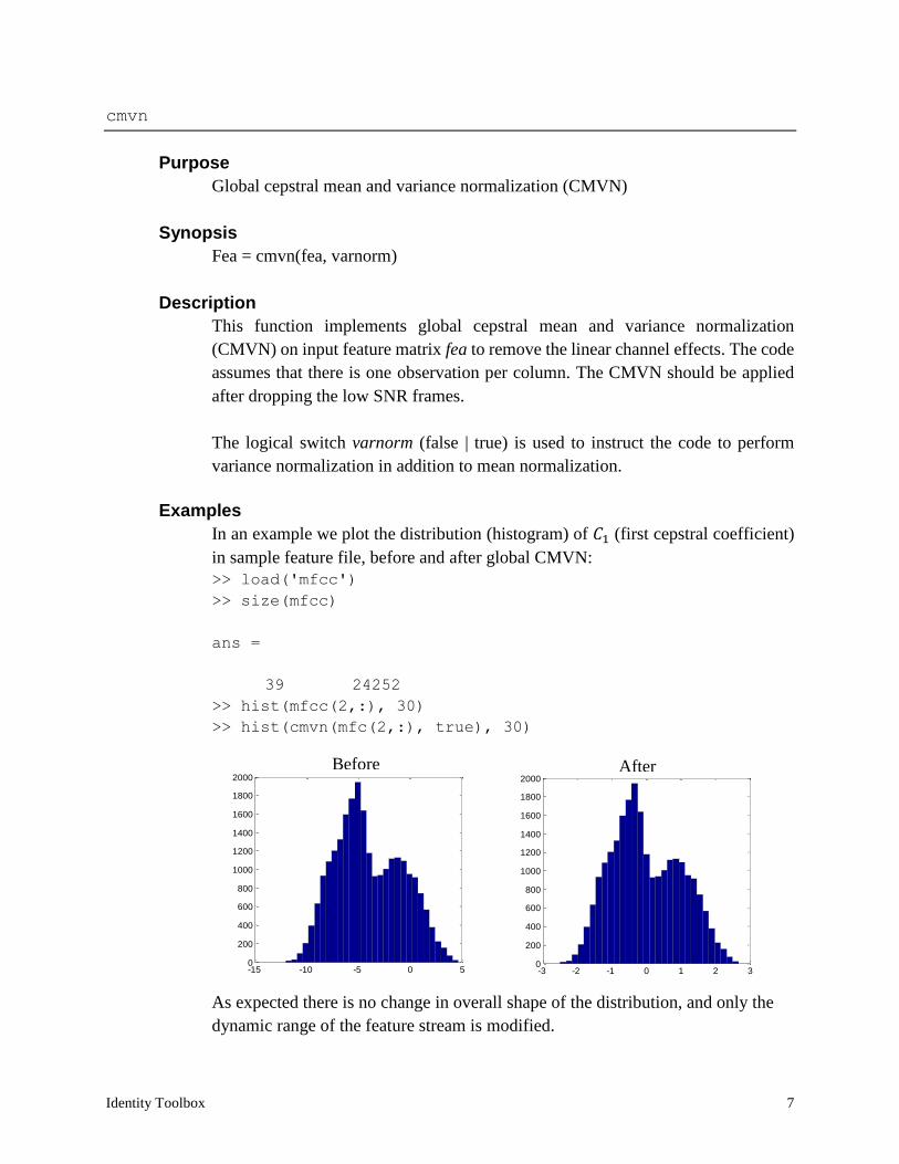
In an example we plot the distribution (histogram) of 𝐶1 (first cepstral coefficient)

in sample feature file, before and after global CMVN:

>> load('mfcc')

>> size(mfcc)

ans =

39 24252

>> hist(mfcc(2,:), 30)

>> hist(cmvn(mfc(2,:), true), 30)

As expected there is no change in overall shape of the distribution, and only the

dynamic range of the feature stream is modified.

-15 -10 -5 0 50

200

400

600

800

1000

1200

1400

1600

1800

2000

-3 -2 -1 0 1 2 30

200

400

600

800

1000

1200

1400

1600

1800

2000

-3 -2 -1 0 1 2 30

200

400

600

800

1000

1200

1400

1600

1800

2000

Before After

8

wcmvn

Purpose

Cepstral mean and variance normalization (CMVN) over a sliding window

Synopsis

Fea = wcmvn(fea, win, varnorm)

Description

This function implements cepstral mean and variance normalization (CMVN) on

input feature matrix fea to remove the (locally) linear channel effects. The code

assumes that there is one observation per column.

The normalization is performed over a sliding window that typically spans 301

frames (that is 3 seconds at a typical 100 Hz frame rate). The middle frame in the

window is normalized based on the mean and variance computed over the specified

time interval. The length of the sliding window can be specified through the scalar

input win which must be an odd number. The CMVN should be applied after

dropping the low SNR frames.

The logical scalar varnorm (false | true) is used to instruct the code to perform

variance normalization in addition to mean normalization. The normalized feature

streams are return in Fea.

Examples

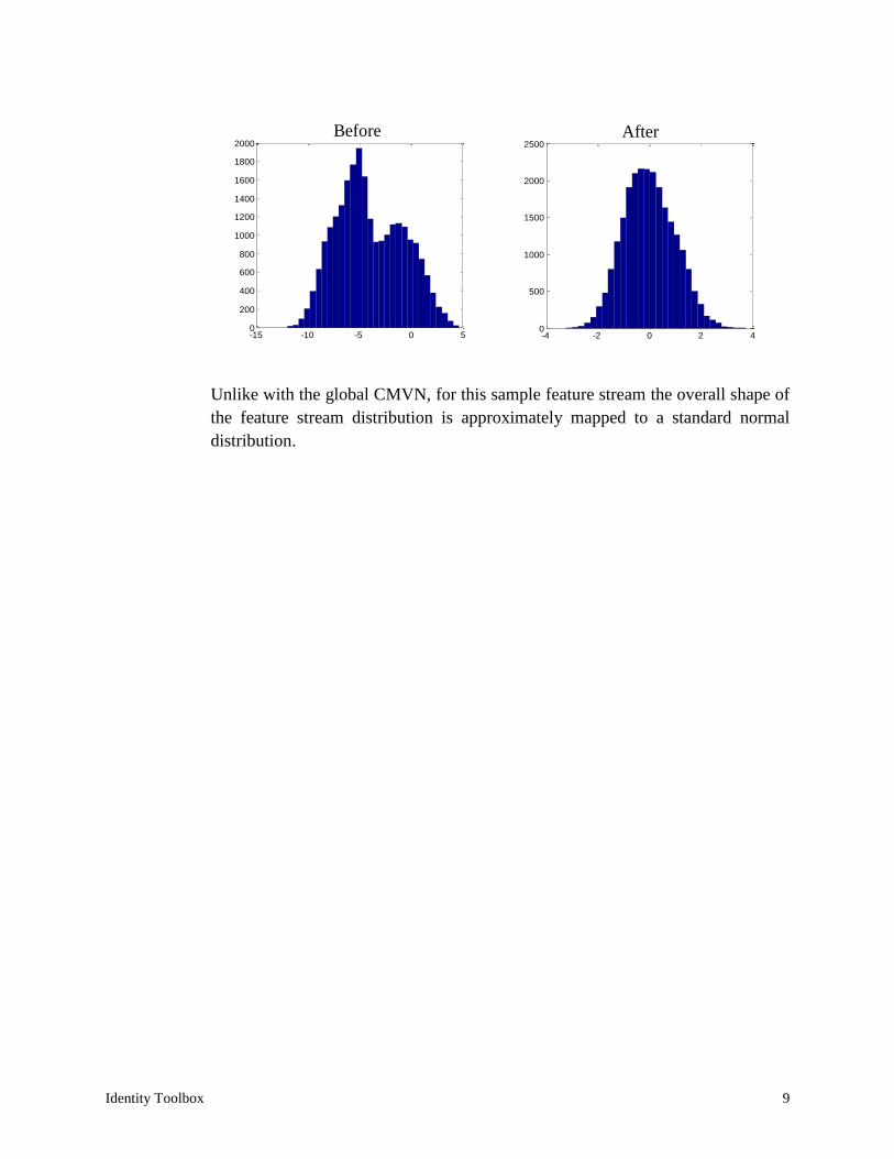
In this example we plot the distribution (histogram) of 𝐶1 (first cepstral coefficient)

in a sample feature file, before and after windowed CMVN:

>> load('mfcc')

>> size(mfcc)

ans =

39 24252

>> hist(mfcc(2,:), 30)

>> hist(wcmvn(mfc(2,:), 301, true), 30)

Identity Toolbox 9

Unlike with the global CMVN, for this sample feature stream the overall shape of

the feature stream distribution is approximately mapped to a standard normal

distribution.

-15 -10 -5 0 50

200

400

600

800

1000

1200

1400

1600

1800

2000

-4 -2 0 2 40

500

1000

1500

2000

2500

-15 -10 -5 0 50

200

400

600

800

1000

1200

1400

1600

1800

2000

Before After

10

fea_warping

Purpose

Short-term Gaussianization over a sliding window (a.k.a feature warping)

Synopsis

Fea = fea_warping(fea, win)

Description

This routine warps the distribution of the cepstral feature streams in fea to the

standard normal distribution (i.e., 𝒩(0, 1)) to mitigate the effects of (locally) linear

channel mismatch. This is specifically useful because the distribution of cepstral

feature streams is often modeled by Gaussians. The code assumes that there is one

observation per column.

The normalization is performed over a sliding window that typically spans 301

frames (that is 3 seconds at a typical 100 Hz frame rate). The middle frame in the

window is normalized based on its rank in a array of sorted feature values over the

specified time interval. The length of the sliding window is specified through the

scalar input win which must be an odd number.

Fea contains the normalized feature streams. Note that the feature warping should

be applied after dropping the low SNR frames.

Examples

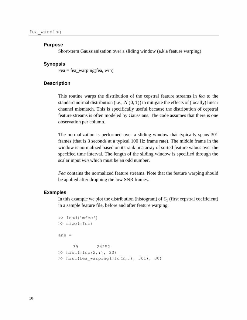
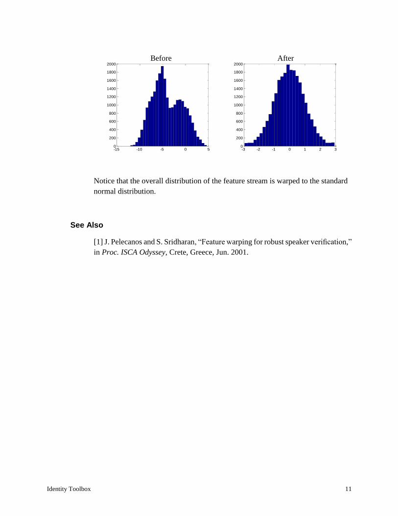
In this example we plot the distribution (histogram) of 𝐶1 (first cepstral coefficient)

in a sample feature file, before and after feature warping:

>> load('mfcc')

>> size(mfcc)

ans =

39 24252

>> hist(mfcc(2,:), 30)

>> hist(fea_warping(mfc(2,:), 301), 30)

Identity Toolbox 11

Notice that the overall distribution of the feature stream is warped to the standard

normal distribution.

See Also

[1] J. Pelecanos and S. Sridharan, “Feature warping for robust speaker verification,”

in Proc. ISCA Odyssey, Crete, Greece, Jun. 2001.

-15 -10 -5 0 50

200

400

600

800

1000

1200

1400

1600

1800

2000

-3 -2 -1 0 1 2 30

200

400

600

800

1000

1200

1400

1600

1800

2000

Before After

12

gmm_em

Purpose

Fit a Gaussian mixture model (GMM) to observations

Synopsis

gmm = gmm_em(dataList, nmix, final_niter, ds_factor, nworkers, gmmFilename)

Description

This function fits a GMM to acoustic feature vectors using binary splitting and

expectation-maximization (EM). The input argument dataList can be either the

name of an ASCII list containing feature file names (assuming one file per line), or

a cell array containing features (assuming one feature matrix per cell). In case a list

of files (the former option) is provided, the features must be saved in uncompressed

HTK format. In case a cell array of features is provided, the function assumes one

observation per column.

The scalar nmix specifies the number of desired components in the GMM, and must

be a power of 2. A binary splitting procedure is used to boot up the GMM from a

single component to nmix components. After each split the model is re-estimated

several times using the EM algorithm. The number of EM iterations at each split is

gradually increased from 1 to final_niter (scalar) for the nmix component GMM.

While booting up a GMM (from one to nmix components) on a large number of

observations, it is practical to down-sample (sub-sample) the acoustic features. It is

usually not necessary to re-estimate the model parameters at each split using all

feature frames. This is due to the redundancy of speech frames and the fact that the

analysis frames are overlapping. The scalar argument ds_factor specifies the down-

sampling factor. The value assigned to the ds_factor is reset to one in the last two

splits.

The scalar argument nworkers specifies the number of MATLAB parallel workers

in the parfor loop. MATLAB by default sets the number of workers to the number

of Cores (not virtual processors!) available on a computer. At the time of writing

this report, MATLAB only supports a maximum of 12 workers on a local machine.

The optional argument gmmFilename (string) specifies the file name of GMM

model to be saved. If this is specified, the GMM hyper-parameters (as structure

fields, see below) are saved in a .mat file on disk.

Identity Toolbox 13

The model hyper-parameters are returned in gmm which is a structure with three

fields:

- gmm.mu component means

- gmm.sigma component covariance matrices

- gmm.w component weights

The code reports the accumulated likelihood of observations given the model in

each EM iteration. It also reports the elapsed time for each iteration.

14

mapAdapt

Purpose

Adapt a speaker specific GMM from a universal background model (UBM)

Synopsis

gmm = mapAdapt(dataList, ubm, tau, config, gmmFilename)

Description

This routine adapts a speaker specific GMM from a UBM using maximum a

posteriori (MAP) estimation. The adaptation data is specified input via dataList,

which should be either the name of an ASCII list containing feature file names

(assuming one file per line), or a cell array containing features (assuming one

feature matrix per cell). In case a list of files is provided, the features must be saved

in uncompressed HTK format.

The input argument ubm can be either a file name (string) or a structure with UBM

hyper-parameters (in form of gmm.mu, gmm.sigma, and gmm.w, see also

gmm_em). The UBM file should be a .mat file with the same structure as above.

The code supports adaptation of all model hyper-parameters (i.e., means,

covariance matrices, and weights). The input string parameter config is used to

specify which parameters should be adapted. Any sensible combination of ‘m’, ‘v’,

and ‘w’ is accepted (default is mean ‘m’). The MAP adaptation relevance factor is

set via the scalar input tau.

The optional argument gmmFilename (string) specifies the file name of the adapted

GMM model to be saved. If this is specified, the GMM hyper-parameters (as

structure fields, see below) are saved in a .mat file on disk.

The model hyper-parameters are returned in gmm, which is a structure with three

fields (i.e., gmm.mu, gmm.sigma, gmm.w).

See Also

[1] D.A. Reynolds, T.F. Quatieri, R.B. Dunn, “Speaker verification using adapted

Gaussian mixture models”, Digital Signal Processing, vol. 10, pp. 19-41, Jan. 2000.

Identity Toolbox 15

score_gmm_trials

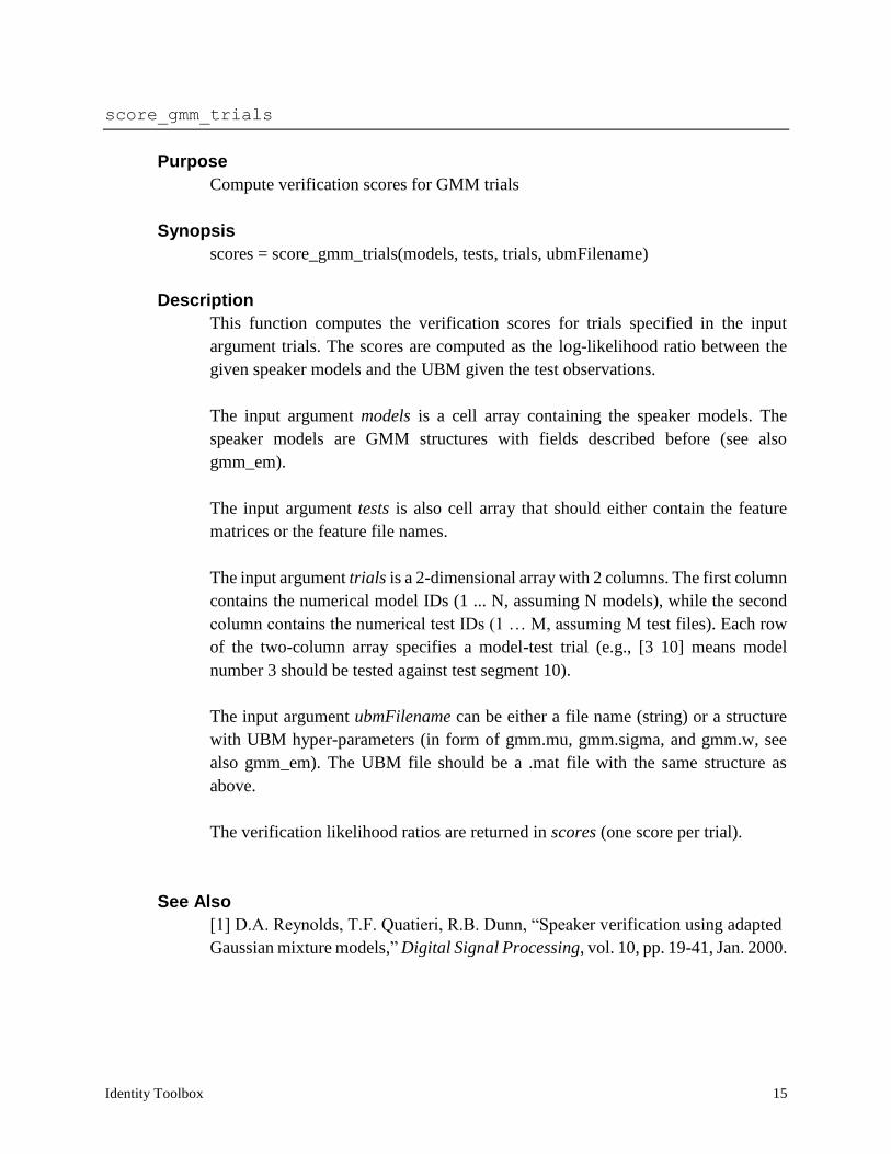
Purpose

Compute verification scores for GMM trials

Synopsis

scores = score_gmm_trials(models, tests, trials, ubmFilename)

Description

This function computes the verification scores for trials specified in the input

argument trials. The scores are computed as the log-likelihood ratio between the

given speaker models and the UBM given the test observations.

The input argument models is a cell array containing the speaker models. The

speaker models are GMM structures with fields described before (see also

gmm_em).

The input argument tests is also cell array that should either contain the feature

matrices or the feature file names.

The input argument trials is a 2-dimensional array with 2 columns. The first column

contains the numerical model IDs (1 ... N, assuming N models), while the second

column contains the numerical test IDs (1 … M, assuming M test files). Each row

of the two-column array specifies a model-test trial (e.g., [3 10] means model

number 3 should be tested against test segment 10).

The input argument ubmFilename can be either a file name (string) or a structure

with UBM hyper-parameters (in form of gmm.mu, gmm.sigma, and gmm.w, see

also gmm_em). The UBM file should be a .mat file with the same structure as

above.

The verification likelihood ratios are returned in scores (one score per trial).

See Also

[1] D.A. Reynolds, T.F. Quatieri, R.B. Dunn, “Speaker verification using adapted

Gaussian mixture models,” Digital Signal Processing, vol. 10, pp. 19-41, Jan. 2000.

16

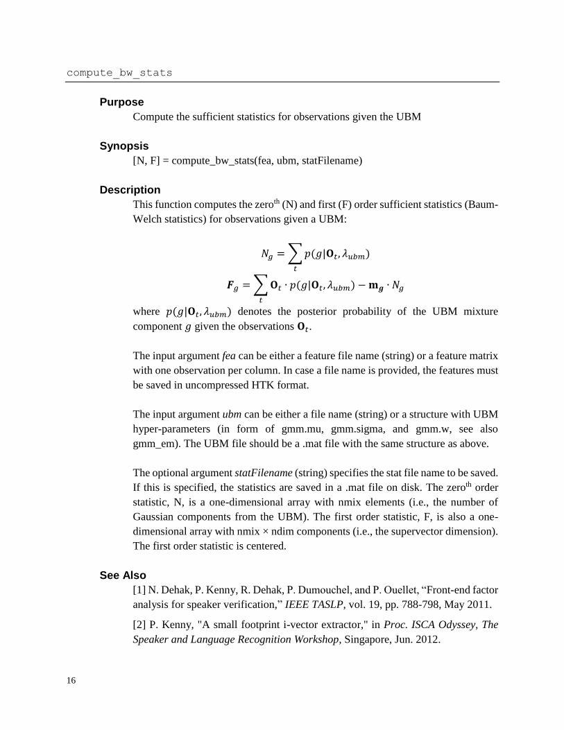
compute_bw_stats

Purpose

Compute the sufficient statistics for observations given the UBM

Synopsis

[N, F] = compute_bw_stats(fea, ubm, statFilename)

Description

This function computes the zeroth (N) and first (F) order sufficient statistics (Baum-

Welch statistics) for observations given a UBM:

𝑁𝑔 = ∑ 𝑝(𝑔|𝐎𝑡, 𝜆𝑢𝑏𝑚)

𝑡

𝑭𝑔 = ∑ 𝐎𝑡 ∙ 𝑝(𝑔|𝐎𝑡, 𝜆𝑢𝑏𝑚)

𝑡

− 𝐦𝒈 ∙ 𝑁𝑔

where 𝑝(𝑔|𝐎𝑡, 𝜆𝑢𝑏𝑚) denotes the posterior probability of the UBM mixture

component 𝑔 given the observations 𝐎𝑡.

The input argument fea can be either a feature file name (string) or a feature matrix

with one observation per column. In case a file name is provided, the features must

be saved in uncompressed HTK format.



gmm_em). The UBM file should be a .mat file with the same structure as above.

The optional argument statFilename (string) specifies the stat file name to be saved.

If this is specified, the statistics are saved in a .mat file on disk. The zeroth order

statistic, N, is a one-dimensional array with nmix elements (i.e., the number of

Gaussian components from the UBM). The first order statistic, F, is also a one-

dimensional array with nmix × ndim components (i.e., the supervector dimension).

The first order statistic is centered.

See Also

[1] N. Dehak, P. Kenny, R. Dehak, P. Dumouchel, and P. Ouellet, “Front-end factor

analysis for speaker verification,” IEEE TASLP, vol. 19, pp. 788-798, May 2011.

[2] P. Kenny, "A small footprint i-vector extractor," in Proc. ISCA Odyssey, The

Speaker and Language Recognition Workshop, Singapore, Jun. 2012.

Identity Toolbox 17

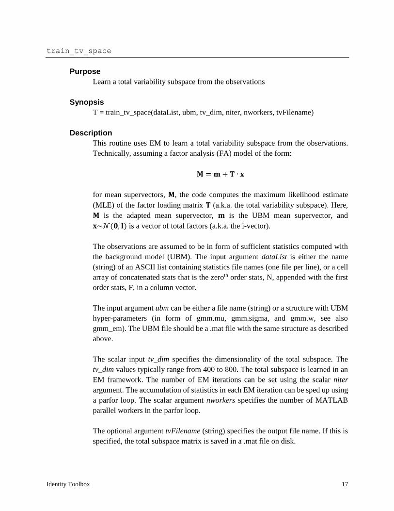
train_tv_space

Purpose

Learn a total variability subspace from the observations

Synopsis

T = train_tv_space(dataList, ubm, tv_dim, niter, nworkers, tvFilename)

Description

This routine uses EM to learn a total variability subspace from the observations.

Technically, assuming a factor analysis (FA) model of the form:

𝐌 = 𝐦 + 𝐓 ∙ 𝐱

for mean supervectors, 𝐌, the code computes the maximum likelihood estimate

(MLE) of the factor loading matrix 𝐓 (a.k.a. the total variability subspace). Here,

𝐌 is the adapted mean supervector, 𝐦 is the UBM mean supervector, and

𝐱~𝒩(𝟎, 𝐈) is a vector of total factors (a.k.a. the i-vector).

The observations are assumed to be in form of sufficient statistics computed with

the background model (UBM). The input argument dataList is either the name

(string) of an ASCII list containing statistics file names (one file per line), or a cell

array of concatenated stats that is the zeroth order stats, N, appended with the first

order stats, F, in a column vector.



gmm_em). The UBM file should be a .mat file with the same structure as described

above.

The scalar input tv_dim specifies the dimensionality of the total subspace. The

tv_dim values typically range from 400 to 800. The total subspace is learned in an

EM framework. The number of EM iterations can be set using the scalar niter

argument. The accumulation of statistics in each EM iteration can be sped up using

a parfor loop. The scalar argument nworkers specifies the number of MATLAB

parallel workers in the parfor loop.

The optional argument tvFilename (string) specifies the output file name. If this is

specified, the total subspace matrix is saved in a .mat file on disk.

18

See Also

[1] D. Matrouf, N. Scheffer, B. Fauve, J.-F. Bonastre, “A straightforward and

efficient implementation of the factor analysis model for speaker verification,” in

Proc. INTERSPEECH, Antwerp, Belgium, Aug. 2007, pp. 1242-1245.



[3] P. Kenny, “A small footprint i-vector extractor,” in Proc. ISCA Odyssey, The


[4] “Joint Factor Analysis Matlab Demo,” 2008. [Online]. Available:

http://speech.fit.vutbr.cz/software/joint-factor-analysis-matlab-demo/.

Identity Toolbox 19

extract_ivector

Purpose

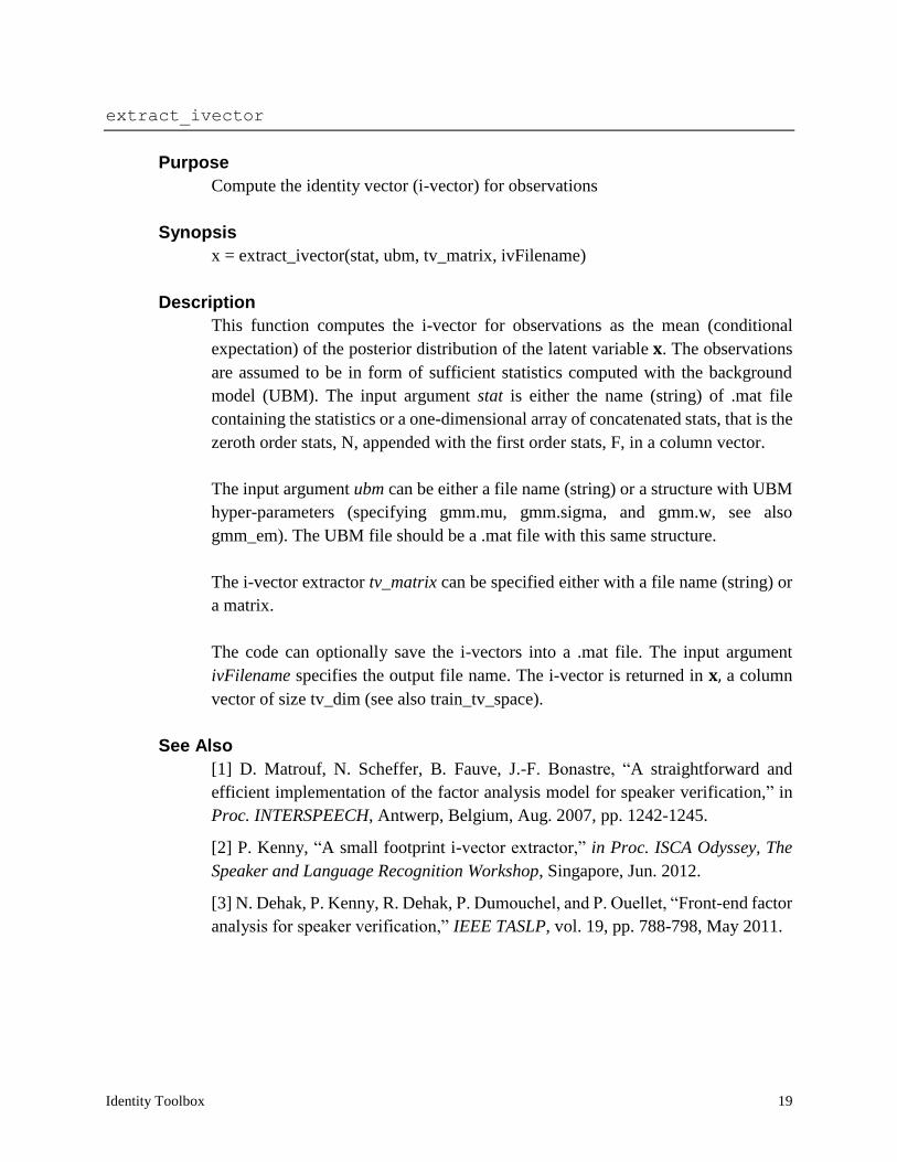
Compute the identity vector (i-vector) for observations

Synopsis

x = extract_ivector(stat, ubm, tv_matrix, ivFilename)

Description

This function computes the i-vector for observations as the mean (conditional

expectation) of the posterior distribution of the latent variable 𝐱. The observations

are assumed to be in form of sufficient statistics computed with the background

model (UBM). The input argument stat is either the name (string) of .mat file

containing the statistics or a one-dimensional array of concatenated stats, that is the

zeroth order stats, N, appended with the first order stats, F, in a column vector.


hyper-parameters (specifying gmm.mu, gmm.sigma, and gmm.w, see also

gmm_em). The UBM file should be a .mat file with this same structure.

The i-vector extractor tv_matrix can be specified either with a file name (string) or

a matrix.

The code can optionally save the i-vectors into a .mat file. The input argument

ivFilename specifies the output file name. The i-vector is returned in 𝐱, a column

vector of size tv_dim (see also train_tv_space).

See Also

[1] D. Matrouf, N. Scheffer, B. Fauve, J.-F. Bonastre, “A straightforward and

efficient implementation of the factor analysis model for speaker verification,” in

Proc. INTERSPEECH, Antwerp, Belgium, Aug. 2007, pp. 1242-1245.

[2] P. Kenny, “A small footprint i-vector extractor,” in Proc. ISCA Odyssey, The




20

lda

Purpose

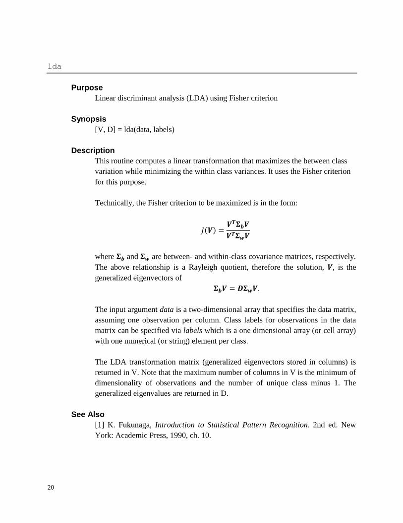
Linear discriminant analysis (LDA) using Fisher criterion

Synopsis

[V, D] = lda(data, labels)

Description

This routine computes a linear transformation that maximizes the between class

variation while minimizing the within class variances. It uses the Fisher criterion

for this purpose.

Technically, the Fisher criterion to be maximized is in the form:

𝐽(𝑽) =𝑽𝑻𝚺𝒃𝑽

𝑽𝑻𝚺𝒘𝑽

where 𝚺𝒃 and 𝚺𝒘 are between- and within-class covariance matrices, respectively.

The above relationship is a Rayleigh quotient, therefore the solution, 𝑽, is the

generalized eigenvectors of

𝚺𝒃𝑽 = 𝑫𝚺𝒘𝑽.

The input argument data is a two-dimensional array that specifies the data matrix,

assuming one observation per column. Class labels for observations in the data

matrix can be specified via labels which is a one dimensional array (or cell array)

with one numerical (or string) element per class.

The LDA transformation matrix (generalized eigenvectors stored in columns) is

returned in V. Note that the maximum number of columns in V is the minimum of

dimensionality of observations and the number of unique class minus 1. The

generalized eigenvalues are returned in D.

See Also

[1] K. Fukunaga, Introduction to Statistical Pattern Recognition. 2nd ed. New

York: Academic Press, 1990, ch. 10.

Identity Toolbox 21

gplda_em

Purpose

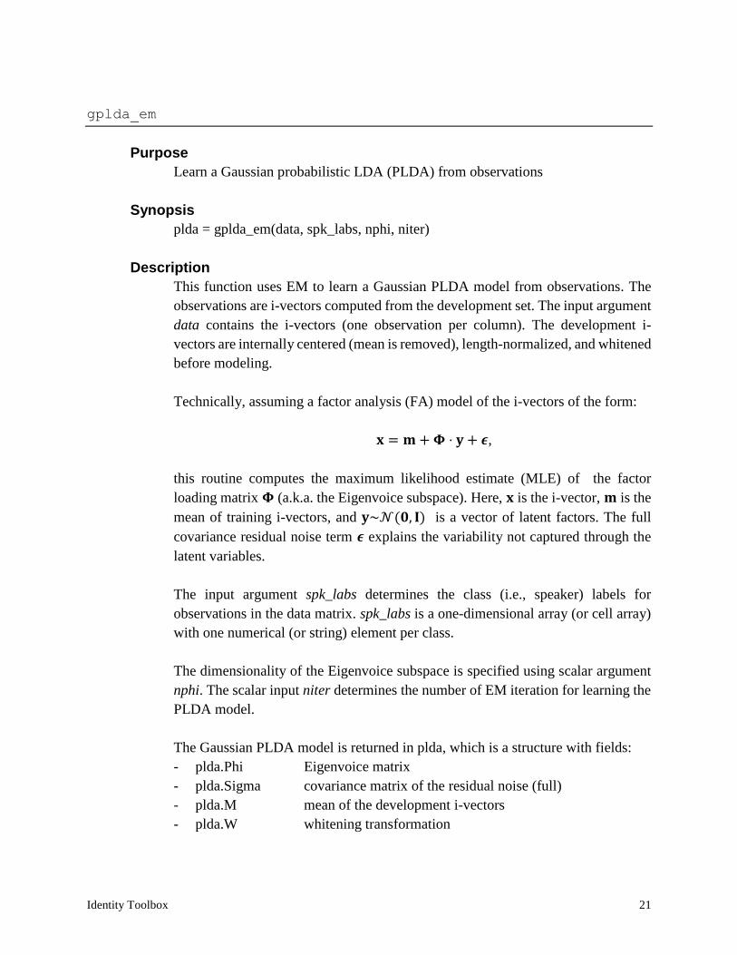
Learn a Gaussian probabilistic LDA (PLDA) from observations

Synopsis

plda = gplda_em(data, spk_labs, nphi, niter)

Description

This function uses EM to learn a Gaussian PLDA model from observations. The

observations are i-vectors computed from the development set. The input argument

data contains the i-vectors (one observation per column). The development i-

vectors are internally centered (mean is removed), length-normalized, and whitened

before modeling.

Technically, assuming a factor analysis (FA) model of the i-vectors of the form:

𝐱 = 𝐦 + 𝚽 ⋅ 𝐲 + 𝝐,

this routine computes the maximum likelihood estimate (MLE) of the factor

loading matrix 𝚽 (a.k.a. the Eigenvoice subspace). Here, 𝐱 is the i-vector, 𝐦 is the

mean of training i-vectors, and 𝐲~𝒩(𝟎, 𝐈) is a vector of latent factors. The full

covariance residual noise term 𝝐 explains the variability not captured through the

latent variables.

The input argument spk_labs determines the class (i.e., speaker) labels for

observations in the data matrix. spk_labs is a one-dimensional array (or cell array)

with one numerical (or string) element per class.

The dimensionality of the Eigenvoice subspace is specified using scalar argument

nphi. The scalar input niter determines the number of EM iteration for learning the

PLDA model.

The Gaussian PLDA model is returned in plda, which is a structure with fields:

- plda.Phi Eigenvoice matrix

- plda.Sigma covariance matrix of the residual noise (full)

- plda.M mean of the development i-vectors

- plda.W whitening transformation

22

See Also

[1] S.J.D. Prince and J.H. Elder, “Probabilistic linear discriminant analysis for

inferences about identity,” in Proc. IEEE ICCV, Rio de Janeiro, Brazil, Oct. 2007.

[2] D. Garcia-Romero and C.Y. Espy-Wilson, “Analysis of i-vector length

normalization in speaker recognition systems,” in Proc. INTERSPEECH, Florence,

Italy, Aug. 2011, pp. 249-252.

[3] P. Kenny, “Bayesian speaker verification with heavy-tailed priors,” in Proc.

Odyssey, The Speaker and Language Recognition Workshop, Brno, Czech

Republic, Jun. 2010.

Identity Toolbox 23

score_gplda_trials

Purpose

Compute verification scores for i-vector trials using the PLDA model

Synopsis

scores = score_gplda_trials(plda, model_iv, test_iv)

Description

This function computes the verification scores for all possible model-test i-vector

trials. The scores are computed as the “batch” log-likelihood ratio between the same

(𝐻1) versus different (𝐻0) speaker models hypotheses:

𝑙𝑙𝑟 = ln𝑝(𝐱1, 𝐱2|𝐻1)

𝑝(𝐱1|𝐻0) ∙ 𝑝(𝐱2|𝐻0)

The i-vectors, 𝐱, are modeled with a Gaussian PLDA provided via plda. The input

plda model is a structure with PLDA hyperparameters (i.e., plda.Phi, plda.Sigma,

plda.M, and plda.W).

Before computing the verification scores, the enrollment and test i-vectors are

internally mean- and length-normalized and whitened. The input arguments

model_iv and test_iv are two-dimensional arrays (one observation per column)

containing unprocessed enrollment and test i-vectors, respectively.

The likelihood ratio test has a linear and closed form solution. Therefore, it is

practical to compute the verification scores at once for all possible combination of

model-test i-vectors, and then select a subset of scores according to a trial list. The

output argument scores is a matrix that contains the verification scores for all

possible trials.

See Also

[1] D. Garcia-Romero and C.Y. Espy-Wilson, “Analysis of i-vector length

normalization in speaker recognition systems,” in Proc. INTERSPEECH, Florence,

Italy, Aug. 2011, pp. 249-252.

[2] P. Kenny, “Bayesian speaker verification with heavy-tailed priors,” in Proc.

Odyssey, The Speaker and Language Recognition Workshop, Brno, Czech

Republic, Jun. 2010.

24

compute_eer

Purpose

Compute the equal error rate (EER) performance measure

Synopsis

[eer, dcf08, dcf10] = compute_eer(scores, labels, showfig)

Description

This routine computes the EER given the verification scores for target and impostor

trials. The EER is calculated as the operating point on the detection error tradeoff

(DET) curve where the false-alarm and missed-detection rates are equal.

The input argument scores is a one-dimensional array containing the verification

scores for all target and impostor trials. The trial labels are specified via the

argument labels which can be a one-dimensional binary array (0’s and 1’s for

impostor and target), or a cell array with “target” and “impostor” string labels.

The logical switch showfig (false | true) is used to instruct the code as to whether

the DET curve should be plotted.

The EER is returned in eer (in percent). Additionally, the minimum detection cost

functions (DCF) are computed and returned if the optional output arguments dcf08

and dcf10 are specified. The dcf08 (×100) is computed according to the NIST SRE

2008 cost parameters, while the dcf10 (×100) is calculated based on the NIST SRE

2010 parameters.

See Also

[1] “The NIST year 2008 speaker recognition evaluation plan,” 2008. [Online].

Available: http://www.nist.gov/speech/tests/sre/2008/sre08_evalplan_release4.pdf

[2] “The NIST year 2010 speaker recognition evaluation plan,” 2010. [Online].

Available: http://www.itl.nist.gov/iad/mig/tests/sre/2010/NIST_SRE10_evalplan.r6.pdf

Identity Toolbox 25

Demos

Introduction

We demonstrate the use of this toolbox with two different kinds of demonstrations.

The first example demonstrates that this toolbox can achieve state-of-the-art

performance on a standard identity task, using the TIMIT corpus. The second

demonstration uses artificial data to show the simplest usage cases for the toolbox.

TIMIT Task

In order to demonstrate how the tools in the Identity Toolbox work individually and

when combined together, we provide two sample demos using the TIMIT corpus:

1) demo_gmm_ubm and 2) demo_ivector_plda. The first and the second demo

show how to use the tools to run speaker recognition experiments in a GMM-UBM

and i-vector frameworks, respectively.

A relatively small scale speaker verification task has been designed using speech

material from the TIMIT corpus. There are a total of 630 (192 female and 438 male)

speakers in TIMIT, from which 530 speakers have been selected for background

model training and the remaining 100 (30 female and 70 male) speakers are used

for tests. There are 10 short sentences per speaker in TIMIT. For background model

training all sentences from all 530 speakers (i.e., 5300 speech recordings in total)

are used. For speaker-specific model training 9 out of 10 sentences per speaker are

selected and the remaining 1 sentence is kept for tests. Verification trials consist of

all possible model-test combinations, resulting in a total of 10,000 trials (100 target

versus 9900 impostor trials).

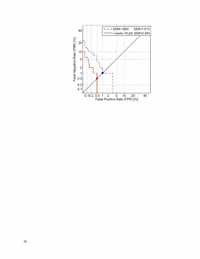
The figure below shows the detection error tradeoff (DET) curves for the two

systems: GMM-UBM (solid) and i-vector-PLDA (dashed). Also shown in the

figure are the system performances on the TIMIT task in terms of the EER. The

EER operating points are circled as the intersection of a diagonal line with the DET

curves.

Identity Toolbox 27

Demos

Artificial Task

A small-scale task generates artificial features for 20 speakers. Each speaker has 10

sessions (channels) and each session is 1000 frames long (which translates to 10

seconds assuming a frame rate of 100 Hz).

The following script (demo_create_data.m) generates the features used in the

following demonstrations:

nSpeakers = 20;

nDims = 13; % dimensionality of feature vectors

nMixtures = 32; % How many mixtures used to generate data

nChannels = 10; % Number of channels (sessions) per speaker

nFrames = 1000; % Frames per speaker (10 seconds assuming 100 Hz)

nWorkers = 1; % Number of parfor workers, if available

rng('default'); % To promote reproducibility.

% Pick random centers for all the mixtures.

mixtureVariance = .10;

channelVariance = .05;

mixtureCenters = randn(nDims, nMixtures, nSpeakers);

channelCenters = randn(nDims, nMixtures, nSpeakers, nChannels)*.1;

trainSpeakerData = cell(nSpeakers, nChannels);

testSpeakerData = cell(nSpeakers, nChannels);

speakerID = zeros(nSpeakers, nChannels);

% Create the random data. Both training and testing data have the same

% layout.

for s=1:nSpeakers

trainSpeechData = zeros(nDims, nMixtures);

testSpeechData = zeros(nDims, nMixtures);

for c=1:nChannels

for m=1:nMixtures

% Create data from mixture m for speaker s

frameIndices = m:nMixtures:nFrames;

nMixFrames = length(frameIndices);

trainSpeechData(:,frameIndices) = ...

randn(nDims, nMixFrames)*sqrt(mixtureVariance) + ...

repmat(mixtureCenters(:,m,s),1,nMixFrames) + ...

repmat(channelCenters(:,m,s,c),1,nMixFrames);

testSpeechData(:,frameIndices) = ...

randn(nDims, nMixFrames)*sqrt(mixtureVariance) + ...

repmat(mixtureCenters(:,m,s),1,nMixFrames) + ...

repmat(channelCenters(:,m,s,c),1,nMixFrames);

end

trainSpeakerData{s, c} = trainSpeechData;

testSpeakerData{s, c} = testSpeechData;

speakerID(s,c) = s; % Keep track of who this is

end

end

28

After generating the features are generated we can use them to train and test GMM-

UBM and i-vector speaker recognition systems.

GMM-UBM Demo

There are four steps involved in training and testing a GMM-UBM speaker

recognition system:

1. Training a UBM from the background data

2. MAP adapting speaker models from the UBM using enrollment data

3. Scoring verification trials

4. Computing the performance measures (e.g., confusion matrix and EER)

The following MATLAB script (demo_gmm_ubm_artificial.m) generates a UBM

speaker-recognition model and tests it:

%%

rng('default')

% Step1: Create the universal background model from all the

% training speaker data

nmix = nMixtures; % In this case, we know the # of mixtures needed

final_niter = 10;

ds_factor = 1;

ubm = gmm_em(trainSpeakerData(:), nmix, final_niter, ds_factor, ...

nWorkers);

%%

% Step2: Now adapt the UBM to each speaker to create GMM speaker model.

map_tau = 10.0;

config = 'mwv';

gmm = cell(nSpeakers, 1);

for s=1:nSpeakers

gmm{s} = mapAdapt(trainSpeakerData(s, :), ubm, map_tau, config);

end

%%

% Step3: Now calculate the score for each model versus each speaker's

% data.

% Generate a list that tests each model (first column) against all the

% testSpeakerData.

trials = zeros(nSpeakers*nChannels*nSpeakers, 2);

answers = zeros(nSpeakers*nChannels*nSpeakers, 1);

for ix = 1 : nSpeakers,

b = (ix-1)*nSpeakers*nChannels + 1;

e = b + nSpeakers*nChannels - 1;

trials(b:e, :) = [ix * ones(nSpeakers*nChannels, 1), ...

(1:nSpeakers*nChannels)'];

answers((ix-1)*nChannels+b : (ix-1)*nChannels+b+nChannels-1) = 1;

Identity Toolbox 29

end

gmmScores = score_gmm_trials(gmm, reshape(testSpeakerData', ...

nSpeakers*nChannels,1), trials, ubm);

%%

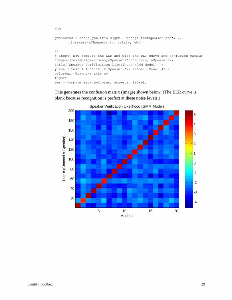
% Step4: Now compute the EER and plot the DET curve and confusion matrix

imagesc(reshape(gmmScores,nSpeakers*nChannels, nSpeakers))

title('Speaker Verification Likelihood (GMM Model)');

ylabel('Test # (Channel x Speaker)'); xlabel('Model #');

colorbar; drawnow; axis xy

figure

eer = compute_eer(gmmScores, answers, false);

This generates the confusion matrix (image) shown below. (The EER curve is

blank because recognition is perfect at these noise levels.)

Speaker Verification Likelihood (GMM Model)

Test

# (

Channel x S

peaker)

Model #

5 10 15 20

20

40

60

80

100

120

140

160

180

200

-4

-3

-2

-1

0

1

2

3

4

5

30

i-vector Demo

There are five steps involved in training and testing an i-vector speaker recognition

system:

1. Training a UBM from the background data

2. Learning a total variability subspace from background statistics

3. Training a Gaussian PLDA model with development i-vectors

4. Scoring verification trials with model and test i-vectors

5. Computing the performance measures (e.g., EER and confusion matrix)

The following MATLAB script (demo_ivector_plda_artificial.m) demonstrates the

use of the i-vector code and shows simple results:

%%

rng('default');

% Step1: Create the universal background model from all the

% training speaker data

nmix = nMixtures;% In this case, we know the # of mixtures needed

final_niter = 10;

ds_factor = 1;

ubm = gmm_em(trainSpeakerData(:), nmix, final_niter, ...

ds_factor, nWorkers);

%%

% Step2.1: Calculate the statistics needed for the iVector model.

stats = cell(nSpeakers, nChannels);

for s=1:nSpeakers

for c=1:nChannels

[N,F] = compute_bw_stats(trainSpeakerData{s,c}, ubm);

stats{s,c} = [N; F];

end

end

% Step2.2: Learn the total variability subspace from all the

speaker data.

tvDim = 100;

niter = 5;

T = train_tv_space(stats(:), ubm, tvDim, niter, nWorkers);

%

% Now compute the ivectors for each speaker and channel.

% The result is size

% tvDim x nSpeakers x nChannels

devIVs = zeros(tvDim, nSpeakers, nChannels);

for s=1:nSpeakers

for c=1:nChannels

Identity Toolbox 31

devIVs(:, s, c) = extract_ivector(stats{s, c}, ubm, T);

end

end

%%

% Step3.1: Now do LDA on the iVectors to find the dimensions that

% matter.

ldaDim = min(100, nSpeakers-1);

devIVbySpeaker = reshape(devIVs, tvDim, nSpeakers*nChannels);

[V,D] = lda(devIVbySpeaker, speakerID(:));

finalDevIVs = V(:, 1:ldaDim)' * devIVbySpeaker;

% Step3.2: Now train a Gaussian PLDA model with development

% i-vectors

nphi = ldaDim; % should be <= ldaDim

niter = 10;

pLDA = gplda_em(finalDevIVs, speakerID(:), nphi, niter);

%%

% Step4.1: OK now we have the channel and LDA models. Let's build

% actual speaker

% models. Normally we do that with new enrollment data, but now

% we'll just reuse the development set.

averageIVs = mean(devIVs, 3); % Average IVs across channels.

modelIVs = V(:, 1:ldaDim)' * averageIVs;

% Step4.2: Now compute the ivectors for the test set

% and score the utterances against the models

testIVs = zeros(tvDim, nSpeakers, nChannels);

for s=1:nSpeakers

for c=1:nChannels

[N, F] = compute_bw_stats(testSpeakerData{s, c}, ubm);

testIVs(:, s, c) = extract_ivector([N; F], ubm, T);

end

end

testIVbySpeaker = reshape(permute(testIVs, [1 3 2]), ...

tvDim, nSpeakers*nChannels);

finalTestIVs = V(:, 1:ldaDim)' * testIVbySpeaker;

%%

% Step5: Now score the models with all the test data.

ivScores = score_gplda_trials(pLDA, modelIVs, finalTestIVs);

imagesc(ivScores)

title('Speaker Verification Likelihood (iVector Model)');

xlabel('Test # (Channel x Speaker)'); ylabel('Model #');

colorbar; axis xy; drawnow;

answers = zeros(nSpeakers*nChannels*nSpeakers, 1);

32

for ix = 1 : nSpeakers,

b = (ix-1)*nSpeakers*nChannels + 1;

answers((ix-1)*nChannels+b : (ix-1)*nChannels+b+nChannels-1)

= 1;

end

ivScores = reshape(ivScores', nSpeakers*nChannels* nSpeakers, 1);

figure;

eer = compute_eer(ivScores, answers, false);

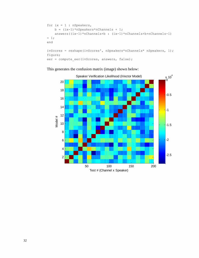
This generates the confusion matrix (image) shown below:

Speaker Verification Likelihood (iVector Model)

Test # (Channel x Speaker)

Model #

50 100 150 200

2

4

6

8

10

12

14

16

18

20

-2.5

-2

-1.5

-1

-0.5

0x 10

4

msr identity toolbox - microsoft.com · identity toolbox 1 msr identity toolbox: a matlab toolbox...

Documents