msc mathematical trading &...

MSc MATHEMATICAL TRADING & FINANCE

“Implementation of Variance Swaps in Dispersion Trading Strategies”

by

Sonesh Ganatra

Part-time student 2002-2004

Supervisor

Dr J.HATGIOANNIDES

CONFIDENTIAL

Sonesh Ganatra 2 of 42

Dedicated to my late father


CONTENTS

Page Acknowledgements 4

Abstract 5

Introduction 6

Chapter 1 : Introducing dispersion trading 1.1 Concept of dispersion trading 10 1.2 Basket Options 13 1.3 Implied Correlation 15 1.4 Issues with the execution of dispersion trades 21 Chapter 2 : Variance swaps 2.1 How the variance swap works 25 2.2 Methodology for pricing Variance swaps 26 Chapter 3 : Implementing the dispersion trading strategy 3.1 Bollinger Bands 30 3.2 Trading Methodology 32 3.3 Presentation of results 35

Conclusion 37 References 39 Appendix 40


Acknowledgements

This dissertation would not have been possible without the guidance of my senior colleagues

at Dresdner Kleinwort Wasserstein.

Special thanks to Alex Capez (Senior Equity Derivatives trader) for being able to spare time to

share his expert knowledge on dispersion trading.

Many thanks also to Georg Bernhard (Quantitative Analyst) for his insight into the topic.

Would also like to express my gratitude to Jocelin Gale (Derivatives structurer), Colin Bennett

(Equity Derivatives Research) and Robert Austin (Equity Derivatives Research) for their help

in retrieving and providing data for this dissertation. Much appreciated.


Abstract

The thesis discusses the calculation and implementation of implied correlation as a

valuation method for the implied volatility of a basket or index option implied volatility. We

suggested how a trader may find a practical application for this useful and relatively simple

tool.

We believe that implied correlation for dispersion trading is an extremely useful and

potentially profitable vehicle for tracing any disparity/inefficiency in the market.

More importantly, we have introduced the concept of using Variance swaps in the execution

of correlation dispersion trades. This is in contrast the more traditional method of trading

strangles on index and basket options. Variance swaps require no delta hedging and are

therefore less operationally intensive than standard delta-hedged option strategies. This

method of trading should not be underestimated and receive merits for its attractive qualities.

Furthermore, we were able to show how Bollinger bands can be used as an indicator to

identify potential trading opportunities. One anticipates that the dispersion strategy outlined

has been designed to generate a consistent return with a low correlation to the underlying

market in a variety of market regimes.

This thesis indicates that using Variance swaps in correlation dispersion trading strategies

can be profitable, but a backtest on a larger number of trades is recommended.


INTRODUCTION


Typically implied correlation is used in dispersion trading to identify opportunities in

which distortion / mispricing of implied volatility has created an identifiable (tradable) gap

between the implied volatility of a benchmark index and its constituent members. The thesis

will explain how this gap can be identified and how to trade dispersion. Implied correlation

also enables better timing for implied volatility investing, as the model provides an indication

of relative value of the constituent members of a basket to its benchmark index.

Dispersion trading has a number of theoretical and practical appeals. While a strict arbitrage

lower bound exists, minimal variance hedging can be used to construct tracking baskets of

options to capitalise on the mispricing of the two different volatility markets that arises from

time to time.

Dispersion trading typically consists of a strategy where one simultaneously sells index

options and buys options on the index components or, conversely, buys index options and

sells options on the underlying stocks. The fundamental theme associated with dispersion

trading is correlation trading.

The value of an index option is determined by the implied volatility of the constituent single

stocks and their cross correlation coefficient. Hence, it is possible to work backwards to derive

how correlated the market estimates the basket of stocks to be. The value of a single stock

option does not take correlation into account as the option is on a single security. If correlation

is less than 100% there is a spread between the index option implied volatility and the basket

implied volatility. In order to calculate index implied volatility from single stock implied volatility

we need to ascertain what level of cross correlation exists between the market weighted

single stocks.

A dispersion trader relies upon the fact that when implied correlation peaks, index implied

volatility is considered to be too high, the trader therefore enters into a trade whereby he/she

sells index implied volatility and simultaneously buys a basket of single stock implied volatility

(market weighted) to hedge his/her short exposure.

In the event that implied correlation troughs the opposite trade is entered in to with a short

position in a basket of market weighted single stock implied volatilities and a simultaneous

long position in index implied volatility as it is considered to be too cheap.

A typical dispersion relative-value position consists of buying single stock volatility, while

selling index volatility. Since the index is composed of single stocks, the two are closely

correlated. The standard dispersion position consists of buying equity at-the-money strangles,

and selling index at-the-money strangles. The total position should be delta-hedged

continuously to achieve the returns expected from arbitrage. However, traditional dispersion

(through calls, puts or strangles) has its failings. Firstly, daily delta hedging entails replication


errors and transaction costs. Furthermore, the strategy is path-dependent; depending on the

market’s evolution, the position can become vega-biased (vega-positive/negative), and

develop into a non-hedged volatility position, rather than a play on pure stock correlation

which is the intention of the arbitrage.

A cleaner way to address these shortcomings is to build a position of variance swaps. These

instruments allow traders to effectively build a long/short position that better matches the

desired arbitrage. Unlike the option strategy, the instruments are delta-neutral at all times and

continuous trading is therefore redundant. Variance swaps are a product that investors have,

more recently, been taking advantage of to fine-tune their risk profile and reduce peripheral

risks, such as path-dependency.

The Variance swap market has grown steadily in recent years. The development has primarily

been driven by investor demand to take direct volatility exposure without the cost and

complexity of managing and delta-hedging a vanilla options position. Measuring the size of an

over-the-counter market is, at the best of times difficult, but the market turnover size has been

estimated, measured in options notional equivalent, to be in the proximity of €20 billion a year.

To put this into context, the turnover of listed Eurostoxx 50 options is about €200 billion a

year.

Variance swap liquidity initially developed on equity index underlyings, and more recently the

single-stock variance swap market has begun to open up.

“….as the market for variance swaps has matured, there have been more trades, at narrower

spreads, and with the ability to execute very large transactions. Users are mainly hedge

funds, with occasional insurance companies, endowments and sophisticated pension funds

executing trades….” (Dean Curnutt, head of equity derivatives strategy at Bank of America

Securities).

In the process of its development, the market has attracted dispersion traders who buy and

sell index variance swaps against single-stock variance swaps to take correlation-like

exposures.

This thesis will attempt to illustrate how the calculation and implementation of implied

correlation can be used in volatility-dispersion trading strategies. More importantly, we

introduce the concept of using Variance swaps in the execution of correlation dispersion

trades.


CHAPTER 1

Introducing dispersion trading


1.1 Concept of dispersion trading

Volatility dispersion trading is a popular hedged strategy designed to take advantage

of relative value differences in implied volatilities between an index and a basket of

component stocks, looking for a high degree of dispersion. This strategy typically involves

short option positions on an index, against which long option positions are taken on a set of

components of the index. It is common to see a short straddle or near-ATM strangle on the

index and long similar straddles or strangles on 40% to 50% of the stocks that make up the

index. If maximum dispersion is realized, the strategy will make money on both the long

options on the individual stocks and on the short option position on the index, since the latter

would have moved very little, earning theta. The strategy is evidently a low-premium strategy,

with very low initial Delta with typically positive Vega bias.

The success of the strategy lies in determining which component stocks to pick. At the

simplest level they should account for a large part of the index to keep the net risk low, but at

the same time it is critical to make sure you are buying "cheap" volatility as well as candidates

that are likely to "disperse."

Let’s discuss the types of values that can be employed in the dispersion strategy. These

values enable traders to determine whether current conditions are suitable for a dispersion

trade. We will distinguish amongst these three kinds of values: realized, implied, and

theoretical.

Realized values can be calculated on the basis of historical market data, e.g. prices observed

on the market in the past. For example, values of historical volatility, correlations between

stock prices are realized values.

Implied values are values implied by the option prices observed on the current day in the

market. For example, implied volatility of stock or index is volatility implied by stock/index

option prices, implied index correlation is an internal correlation implied by the market. We

shall discuss this in further detail later on in the chapter.

Theoretical values are values calculated on the basis of some theory, so they depend on the

theory you choose to calculate them. Index volatilities calculated on the basis of the portfolio

risk formula are theoretical, and can differ from realized or implied volatilities.

A comparison of theoretical values with realized ones allows traders to determine what

market behaviour are best applied to the actual trading environment. By studying and

analyzing the historical relationship between these two types of values one can make an

informed decision about related forecasts.


By comparing implied and historical volatilities, theoretical and realized, or theoretical and

implied values of the index risk, one can attempt to ascertain the best time to employ the

dispersion strategy or to choose to continue to monitor the markets.

The dispersion strategy typically consists of short selling options on a stock index while

simultaneously buying options on the component stocks, the reverse dispersion strategy

consist of buying options on a stock index and selling options on a the component stocks.

This is an example of a behavioural/stochastic arbitrage relationship and is the basis of the

dissertation. In other words historical records show an ‘a posteriori’ link between two

derivatives. The relationship is based is principally based on correlation between different

securities/derivatives or some form of dependence, but this association cannot be expected to

resist all kinds of eventualities.

Later on we will discuss the behavioural/stochastic relationship between the two portfolios

(i.e. between index options and the n individual options that are contained in the index). This

arbitrage is called a non-linear index arbitrage, because options have a non-linear payoff

structure.

Figure 1 illustrates the levels of implied and historic volatility on the Eurostoxx 50 Index. It can

clearly be seen historic volatility was greater than implied volatility at times and reached a

local maximum in the last week of September 2001. The explanation for this lies in the tragic

events of September 11. A similar spike in volatility, which was driven by very different

factors, can be observed in September 2002. This particular time was quite good for buying

cheap index options, and thus to engage in the reverse dispersion strategy. Figure 2 displays

the spread between the two measures over the same time horizon.

Figure 1. Levels of 1 month ATM Implied and 30 day historic volatilities on the Eurostoxx 50 Index

5

15

25

35

45

55

65

Mar-99 Sep-99 Mar-00 Sep-00 Mar-01 Sep-01 Mar-02 Sep-02 Mar-03 Sep-03 Mar-04

%

Implied ATM 1 Month Historical 30 Day


Figure 2. Volatility spread between Levels of 1 month ATM Implied and 30 day historic volatilities.

Characteristically, rising equity prices usually have the effect of cooling off the realised

historical volatilities, and the implied volatilities tend to follow or anticipate that move,

especially on the short end of the curve. Conventional wisdom has it that bear market moves

tend to more volatile, with large spiky movements, whereas bull markets tend to be

characterised by a steady appreciation in asset prices.

Empirical evidence has shown that in general implied volatilities on indices typically move

synchronously. The implied volatility index of global equity indices such as the S&P 500, Dax,

CAC40, FTSE100 and Nikkei are virtually coincident, since such indices reflect the state of

economics as a whole, and so their performances are affected by analogous factors.

Another noteworthy point to make is that implied volatilities of global equity indices are lower

than those of sector indices. This can be explained by the fact that changes in one stock

within a sector can potentially have a considerable impact on the index of its sector, but the

change may only have a slight influence on the overall market index. So, risk for an index that

consists of equities from within the same industry is higher.

Major market indices have on the whole lower implied volatility in comparison with sector

indices. But it should not be considered that some indices are better or worse for application

of dispersion strategies. The important role in the strategy is not the absolute value of implied

volatility, but the historical relationship between implied and realised index volatility.

The Eurostoxx 50 index is considered to be the most liquid of all European indices and hence

the focus of our analysis will be primarily based on this.

-25

-15

-5

5

15

25

Mar-99 Sep-99 Mar-00 Sep-00 Mar-01 Sep-01 Mar-02 Sep-02 Mar-03 Sep-03 Mar-04

SPREAD


1.2 Basket Options

Investors are typically interested in arbitrage possibilities between options on an

index and options on the individual stocks. We will briefly discuss the pricing methodology

that market practitioners use to price these options. Determining the price of a basket option

is not a trivial task, because there is no explicit analytical expression available for the

distribution of the weighted sum of the assets in the basket.

An option on such a basket is cheaper than buying options on each of the individual assets in

the basket. The reason is that the volatility of the basket is less than the sum of the individual

asset volatilities, unless the components’ prices are perfectly correlated. Mathematically, this

can be shown with a simple example: a basket that consists of two securities with volatilities

σ1 and σ 2, weights ω1, ω2 and correlated with coefficient ρ. Assuming that each of the assets

exists in a Black Scholes economy and that their prices are distributed lognormally, the

volatility of the basket, σB, is given by,

212121

22

21

21 2 σσωρωσωσωσ ++=B (1)

When the two components are perfectly correlated, ρ = 1, and stocks weighted equally we obtain,

2)(

212

21 212

212121

21

σσσσσσσσσ

+=+=++=B (2)

which is the maximal possible value. (The correlation coefficient lies between minus one and

one, by definition). From the financial perspective, the foregoing simple mathematical

relations demonstrate the idea of diversification. The investor holds the basket to reduce the

risk exposure compared with exposure to the individual assets. Hedging such a position with

a set of options on the individual basket components works against the purpose. It

overhedges the risk and costs too much.

However, to use an option on the basket as a whole, a pricing and hedging methodology is

needed. The first step in using such a methodology consists of adopting a framework of

underlying assumptions, and the most reasonable approach would be a straightforward

extension of the familiar Black-Scholes framework onto the case of multiple assets.

What are possible approaches to pricing basket options in this setting? The simplest solution

would be to treat the basket as a single asset—an index— and use familiar methods such as

the Black-Scholes formula for European calls and puts to price the option.

The basket price at any given time t is a weighted sum of the prices Si(t) of n components,


∑=

=n

iii tSB

1)(ω (3)

where iω are the weights of each asset. We will assume that the world satisfies the

conventional Black-Scholes assumptions, and each of the asset prices )(tSi follows a lognormal stochastic process,

+

−= )(

2exp)(

2

tdWdtStdLnS iii

iii σσµ (4)

where )(tdWi is a Wiener process. The solution of (1.1) is,

+

−= tztStS ii

iiii σσµ

2exp)(

2

(5)

where )0(ii SS = is the ith asset price at trade iσ is the ith annualised volatility iq is the corresponding continuously compounded, annualised dividend yield ii qr −=µ is the mean rate of return on the ith asset in a risk-neutral world

r is the continuously compounded, annualised riskless interest rate and ix is a random variable, normally distributed with mean 0 and variance 1. We shall also assume the logarithms of assets i and j are correlated with coefficient ijρ

i.e. [ ] ijji zzE ρ= . Note that the mean iα and the standard deviation iβ of )(ln tSi are given by,

iiii tSt µα += ln)( tt ii σβ =)( (6)

In this framework, the value of a European option on a basket is given by

−= ∑

=

− 0,)(max1

n

iii

rt KTSEeV ωφ (7)

where T is the option expiry time, K is the strike price, [ ]•E denotes the risk-neutral expectation value, and φ is 1 for a call and –1 for a put. While simplicity is an important advantage, this method has obvious drawbacks. If the basket

components’ prices are lognormally distributed, then assuming that the distribution of basket

prices is also lognormal is inconsistent. An even bigger drawback of this approach is that it

makes it impossible to hedge exposure to the individual volatilities and correlations.

Investors seek arbitrage possibilities between options on an index and options on individual

stocks within the index. The trade based on this strategy is intended to exploit the

discrepancy between the pricing of index options and the portfolio of individual stock options.

This discrepancy can be found in the difference in correlation or volatility in almost equal


portfolios and results in ‘trading correlation’ or ‘trading volatility’. The discrepancy shows

whether the index option or the portfolio of individual options is cheaper or more expensive

than the other. The trading strategies should be insensitive to changes in other option

parameters than the correlation and/or volatility sensitivity. i.e. the position should be hedged

against these parameters. The next section attempts to explain implied correlation.

1.3 Implied Correlation

Implied correlation refers to the average correlation coefficient that adequately

explains the difference between index implied volatility and the average implied volatility of

the constituent stocks relative to their weight in the basket. A value for the expected average

cross correlation coefficient can be extracted from single stock implied volatility and the index

implied volatility.

Typically implied correlation is used in dispersion trading to identify opportunities in which

distortion/mispricing of implied volatility has created an identifiable (tradeable) gap between

the implied volatility of a benchmark index and its constituents members.

Implied correlation also enables better timing for implied volatility investing, as the model

provides an indication of relative value of the constituent members of a basket to he

benchmark index.

The fluctuations seen in the spread between the index volatility and the basket implied

volatility are due to a change in either correlation expectations, a change of basket

constituents or a change on volatility. It is a widespread observation that the spread between

the two narrows in volatile markets as correlation rates tend to rise in volatile or declining

markets.

Figure 3 below plots the implied correlation of the Eurostoxx 50 index components and the

performance of the index itself. Three events have been highlighted. These events saw equity

markets display directional shifts in volatility and simultaneous shifts in implied correlation

rates.

Figure 3. Implied Correlation and index performance of Eurostoxx 50 Index

1800

2300

2800

3300

3800

4300

Jul-01 Jan-02 Jul-02 Jan-03 Jul-03 Jan-04 Jul-04

Inde

x Le

vel

35

45

55

65

75

85

95

Implied C

orrelation (%)

Index LevelImplied Correlation


The chart begins just prior to the tragic events of September 11. As one would expect the

market experienced a sharp, prominent spike in implied correlation as the market declined

sharply over this period. Subsequently, implied correlation remained relatively stable until

global economic indicators began to weigh on the equity markets with concerns over rate cuts

suggesting economic frailty.

By May 2002 equity markets had begun a pattern of decline that was met with a spike in

implied correlation, that peaked when credit ratings were cut on some key financial stocks

(heavily weighted within the index).

The start of 2003 saw markets concerned with the impact of the war in the gulf, this fear

gradually eroded and as it did investors saw implied correlation decrease as the index gained

back old ground.

Knowing at what point correlation and possibly implied volatility begin to decline after an initial

spike in both implied volatility and correlation, are crucial in implementing recovery strategies.

The inverse of this rule is also true in stable or rising markets. Extremities of this rule were

seen in the tech rally when single stock implied volatility rose and correlation remained at

lower levels (mainly due to high diversification in heavily weighted stocks), causing index

implied volatility to remain at subdued levels (relative to the basket).

Much has been written regarding the fact that correlation shares the same trait as implied

volatility and its relationship with volatile stock markets; namely it has a tendency to increase

in volatile markets.

Given this relationship investors have an interest in knowing if risk levels perceived by the

options markets are suggesting an increase or decrease in correlation levels. As higher

implied correlation often corresponds to fast markets where gains can be translated to losses

in a rapid motion.

Academics believe that there is a relationship between index implied volatility and implied

correlation, e.g. a high implied correlation results in high index implied volatility and vice

versa. This is illustrated in Figure 4 that plots a scatter chart of the 60 day implied correlation

against the 60 day implied volatility for the Eurostoxx Index weekly from Jan 1999 to Sep

2004. The close relationship of implied volatility and correlation is one reason why the topic

generates such a high degree of interest. The causation of high or low levels of implied

correlation is a rather more speculative topic.


Figure 4. Scatter chart of 60 day implied correlation vs 60 implied volatility for the Eurostoxx 50 index.

The reason that dispersion traders employ implied correlation is that implied correlation and

the disparity in implied volatility points between the underlying index and the basket of single

stocks has a strong negatively correlated relationship, hence low implied correlation tends to

equate to higher dispersion and visa versa.

However, the spread between the two sets of implied volatility data does not have a linear

degree of negative correlation so apart from occasions when the two data sets are trading at

parity the trader would have no way of knowing if the spread was at abnormal (i.e. tradeable)

levels.

If for example index implied volatility is at 25% and the basket implied volatility is at 30% then

implied correlation maybe 30%. However, if the same spread (5 vol points) is achieved at

60% index implied volatility and 65% basket implied volatility, implied correlation maybe 50%.

Hence looking just at the spread does not provide enough information to suggest whether

levels are extreme or not.

The dispersion strategy is designed to generate pure alpha by hedging stock market risk and

exploit the mispricing and inefficiencies in the options market. In chapter 3 a strategy will be

proposed whereby focus will be placed on periods when the implied average correlation

deviates from its historical norm. This may offer the investor a potential to profit from using

this strategy.

The general trading rules for the dispersion strategy are as follows:

0

10

20

30

40

50

60

0 10 20 30 40 50 60 70 80 90 100

Implied Correlation

Impl

ied

Vola

tility

(%)


averageimplied ρρ >

When the implied average correlation is greater than the average correlation, index options

may be rich relative to the stock options. The dispersion trade would be to sell the index

options and to buy the individual stock options, ‘sell correlation’.

averageimplied ρρ <

Conversely, when the implied average correlation is less than the average correlation, index

options may be cheap relative to the stock options. The dispersion trade would be to buy the

index options and to sell the individual stock options, ‘buy correlation’. The next section will

discuss the difference between average and implied correlation.

Average Correlation Historical correlation is the determination of the dependence between two stocks on the basis

of their past movements. Before defining the correlation, let us first define the covariance. The

covariance term emerges when calculating the variance of the sum of two variables say,

Z=X+Y,

),(2)()()( YXCovYVarXVarZVar ++= (8)

Application of statistical theory infers that the covariance between stock x and y can be

estimated as follows,

∑=

−− −−−

==m

ktyktytxktxtxyt RRRR

myxCov

1,,,,, ))((

11),( σ (9)

Using the above result we can now define the historical correlation between two random

stocks x and y. It is defined as the ratio between the covariance and the individual deviations,

tytx

txytxy

,,

,, σσ

σρ = (10)

it can be estimated as follows,

∑ ∑

∑

= =−−

=−−

−−

−−=

t

k

m

ktyktytxktx

m

ktyktytxktx

txy

RRRR

RRRR

1

2

1,,

2,,

1,,,,

,

)()(

))((ρ (11)

Next consider a portfolio of n stocks. There will exist ½n(n-1) correlations. Using these

pairwise correlations it is possible to define a single, historical ‘average’ correlation for the


basket of constituents stocks. This is simply a question of calculating the weighted average of

pairwise correlations between the individual components,

∑ ∑

∑ ∑

= +=

= +== n

x

n

xyyxxy

n

x

n

xyyxyxxy

avg

1 1

1 1

σσρ

σσωωρρ (12)

Implied Correlation Since there is only one basket price for a basket of n stocks means that it is impossible to

calculate all the implied correlations from a basket option.

It is only possible to calculate the implied average correlation for a basket for which there

exist traded index options and individual options on stocks in the index. Consider first the

volatility of the basket (or index), this can be defined in terms of its component single stock

volatilities as follows,

∑ ∑ ∑= = +=

+=n

x

n

x

n

xyxyyxyxxxI

1 1 1

222 2 ρσσωωσωσ (13)

where,

11

=∑=

n

xxω

We now make an assumption that the correlation for each pairwise component is the same, so ρρ =xy for every x and y.

If the component’s implied volatilities are known then the average implied correlation, ρ , is:

∑ ∑

∑

= +=

=

−= n

x

n

xyyxyx

n

xxxI

1 1

1

222

2 σσωω

σωσρ (14)

In extreme market conditions the implied correlation can exceed 100%. The dispersion strategy above is based on the discrepancy between the implied and the

realized average correlation.

Alternatively to monitoring the spread between implied and average correlation to identify

trading opportunities, a trader could instead monitor the spread of single stock implied

volatility (market weighted) to that of the traded index implied volatility.


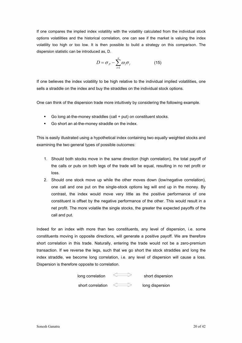
If one compares the implied index volatility with the volatility calculated from the individual stock

options volatilities and the historical correlation, one can see if the market is valuing the index

volatility too high or too low. It is then possible to build a strategy on this comparison. The

dispersion statistic can be introduced as, D.

∑=

−=n

iiiPD

1σωσ (15)

If one believes the index volatility to be high relative to the individual implied volatilities, one

sells a straddle on the index and buy the straddles on the individual stock options.

One can think of the dispersion trade more intuitively by considering the following example.

Go long at-the-money straddles (call + put) on constituent stocks.

Go short an at-the-money straddle on the index.

This is easily illustrated using a hypothetical index containing two equally weighted stocks and

examining the two general types of possible outcomes:

1. Should both stocks move in the same direction (high correlation), the total payoff of

the calls or puts on both legs of the trade will be equal, resulting in no net profit or

loss.

2. Should one stock move up while the other moves down (low/negative correlation),

one call and one put on the single-stock options leg will end up in the money. By

contrast, the index would move very little as the positive performance of one

constituent is offset by the negative performance of the other. This would result in a

net profit. The more volatile the single stocks, the greater the expected payoffs of the

call and put.

Indeed for an index with more than two constituents, any level of dispersion, i.e. some

constituents moving in opposite directions, will generate a positive payoff. We are therefore

short correlation in this trade. Naturally, entering the trade would not be a zero-premium

transaction. If we reverse the legs, such that we go short the stock straddles and long the

index straddle, we become long correlation, i.e. any level of dispersion will cause a loss.

Dispersion is therefore opposite to correlation.

long correlation short dispersion

short correlation long dispersion


1.4 Issues with the execution of dispersion trades

In practice the trade is harder to execute than this theoretical scheme might suggest,

as hedging the single stock part of the trade is fraught with cost and difficulty. Furthermore, to

actually trade entirely (or even partially) the correct market weighted constituents of the single

stock basket exposes the dispersion trader to significant spread risk.

The spread risk is created by the liquidity and hence market makers; if an option is less

popular the market maker widens the volatility spread that he/she is prepared to trade for. In

constructing a market weighted single stock implied volatility basket the dispersion trader

requires very tight spreads that actually reflect the degree of correlation that an underlying

single stock may have with an index, as the spread deviates away from this range then the

whole dispersion trade becomes less economically viable.

For example, stock options are available on all Eurostoxx 50 constituents as well as on the

index itself, making it theoretically possible to implement a perfect directional hedge.

However, stock options on Air Liquide, L’Oreal and several other stocks are considerably less

liquid than most others, which serves to impede implementation. The bottom 6 stocks in terms

of daily option notional turnover account for about 6.6% of the index by weight, which means

they are not insignificant. It is still possible to place the complete trade, but “slippage” is to be

expected, i.e. trading away from the initial price levels. When a trade is required in significant

size, the level of slippage could become unacceptable.

One compromise to reducing spread risk is to limit the number of basket constituents as this

does not materially effect the volatility profile of the basket as it maybe observed that in most

market capitalization weighted indices that 70-80% of the index is represented by 50% of the

index constituents.

# of constituents % weighting of top 50%

DAX 30 83.57 AEX 24 86.16 FTSE 100 102 87.21 Eurostoxx 50 50 71.63 CAC 40 39 81.55

A compromise to overcome spread risk could be:

• Go long at-the-money straddles (calls + puts) on the liquid subset of constituent stocks, with

each straddle weighted in accordance with the constituent’s weight in the index.

• Go short an at-the-money straddle on the index.

Implementing the trade by using only a subset of more liquid index constituents will still give

correlation exposure. However, a directional risk has now opened up. Should the uncovered


stocks rally or decline sharply, their impact will be reflected in the index leg of the trade but

not in the stock leg. There is no limit to the potential downside of the payoff in such

“incomplete” trades.

Another issue that adds to the trading complexity of dispersion trading is that the delta of all

options has to be kept neutral at all times to maintain a pure volatility exposure rather than a

directional one. This will involve constant rolling of positions and dynamically hedging the

basket with futures or stocks, again exposing the dispersion trader to spread risk and cost.

As already pointed out, traders traditionally employ straddles to exploit the variations in

implied volatility and correlation. The position has a delta of close to zero upon initiation,

meaning that the positions pay-off is indifferent to market moves.

However, markets do move and hence the delta neutrality of a straddle position would be

disrupted. As a result the position becomes dependant on the market direction. While the

holder of the straddle has a long gamma position, which benefits them in times of big market

moves, the short straddle investor can get hurt on a short gamma position.

The delta of the straddle position must be dynamically hedged in order for the position to

retain its delta neutrality; a process which is highly cost intensive and often eats up a large

proportion of the potential profit. Additionally, the option position would need to be rolled into

higher or lower strikes depending on whether the market moves up or down to always be as

close-to-the-money as possible, a process which adds up to the costs. Finally the positions

should also be rolled into later expiries to avoid a high gamma exposure towards the end of

the lifetime on an at-the-money option.

There is a third alternative, however, which can be implemented using dynamic hedging, and

can be designed to take advantage of both a correlation and a volatility view. Furthermore,

this trade can be put together without the directional risk highlighted above. The trade would

be:

• Go long at-the-money straddles (calls + puts) on a liquid subset of constituent stocks,

• Go short a variance swap on the index

Variance swaps require no delta hedging and are therefore less operationally intensive than

standard delta-hedged option strategies. Variance swaps trade much more than volatility

swaps because they are easier for the dealer to hedge, and so have much narrower spreads.

For illustration, let us consider a simulation run on the Eurostoxx 50 between late September

2001 and early April 2002. Implied volatilities peaked on 23 September, following dramatic

equity sell-offs. Between late September and the 1 April, equity markets saw a strong

recovery with implied volatilities more than halving.

In the below example, a trader who wanted to take a short volatility position in September

2001 would have sold the closest at-the-money available straddles constructed with one short


call and one short put on the Eurostoxx 50. To reduce gamma and increase liquidity we

assumes that the trader sold options with around 90 days left to maturity and a minimum of 30

days.

The remaining delta position would be hedged with an according position in the future once a

day. As investors are adopting different hedging strategies and face different fees for trading,

we neglected the impact of commission. The chart below plots the theoretical profit and loss

of a delta hedged short-straddle position and a position in a volatility swap with similar

volatility exposure.

Figure 5. Deteriorating effect of a manually delta hedged short-straddle.

Note that the payoff of the variance swap is linearly split over the life of the option in order to

compare the payoffs of both strategies. In practice, a volatility swap will usually be settled

once at the end of its life.

Although both positions were yielding a profit, the payoff of the volatility swap clearly

outperforms that of a delta hedged straddle. While the volatility swap contract gives straight

exposure to realized volatility, the straddle has in practice some unavoidable exposure to the

direction of the underlying, despite the delta hedge.

Another added advantage of the variance swap over the straddle is that the straddle would

have been rolled from one expiry into another three times and from one strike to another over

50 times in order to always pick the ideal at-the-money strike, not to mention the continuous

future hedge which adds additional costs.

Chapter 2 will now examine the concept and pricing methodology of a variance swap.

0

500

1000

1500

2000

2500

Sep-01 Oct-01 Nov-01 Dec-01 Jan-02 Feb-02 Mar-02

delta hedged straddle volatility swap

Payoff


CHAPTER 2

Variance Swaps


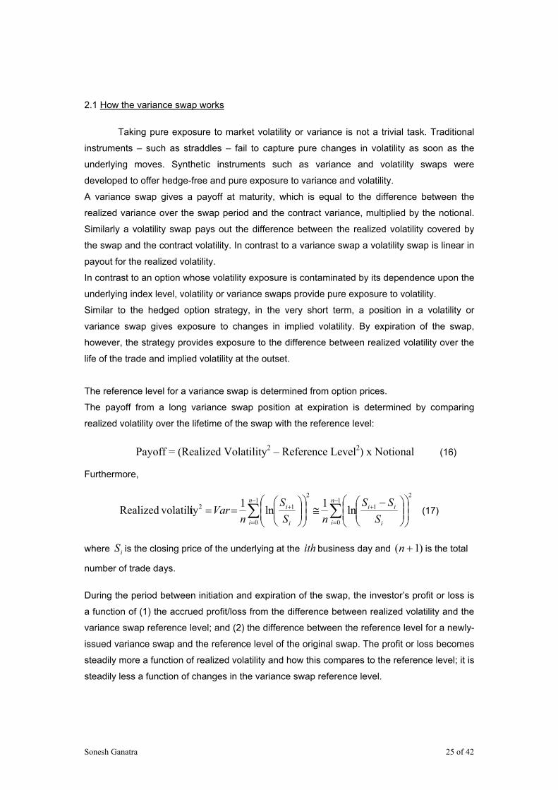
2.1 How the variance swap works

Taking pure exposure to market volatility or variance is not a trivial task. Traditional

instruments – such as straddles – fail to capture pure changes in volatility as soon as the

underlying moves. Synthetic instruments such as variance and volatility swaps were

developed to offer hedge-free and pure exposure to variance and volatility.

A variance swap gives a payoff at maturity, which is equal to the difference between the

realized variance over the swap period and the contract variance, multiplied by the notional.

Similarly a volatility swap pays out the difference between the realized volatility covered by

the swap and the contract volatility. In contrast to a variance swap a volatility swap is linear in

payout for the realized volatility.

In contrast to an option whose volatility exposure is contaminated by its dependence upon the

underlying index level, volatility or variance swaps provide pure exposure to volatility.

Similar to the hedged option strategy, in the very short term, a position in a volatility or

variance swap gives exposure to changes in implied volatility. By expiration of the swap,

however, the strategy provides exposure to the difference between realized volatility over the

life of the trade and implied volatility at the outset.

The reference level for a variance swap is determined from option prices.

The payoff from a long variance swap position at expiration is determined by comparing

realized volatility over the lifetime of the swap with the reference level:

Payoff = (Realized Volatility2 – Reference Level2) x Notional (16)

Furthermore,

21

0

1

21

0

12 ln1ln1ty volatiliRealized ∑∑−

=

+−

=

+

−≅

==

n

i i

iin

i i

i

SSS

nSS

nVar (17)

where iS is the closing price of the underlying at the ith business day and )1( +n is the total

number of trade days.

During the period between initiation and expiration of the swap, the investor’s profit or loss is

a function of (1) the accrued profit/loss from the difference between realized volatility and the

variance swap reference level; and (2) the difference between the reference level for a newly-

issued variance swap and the reference level of the original swap. The profit or loss becomes

steadily more a function of realized volatility and how this compares to the reference level; it is

steadily less a function of changes in the variance swap reference level.


Unlike options, variance swaps cost zero to enter into, since the variance swap rate

represents the risk-neutral expected value of the realized return variance.

Variance swaps are offered on most benchmark indices, but variance swaps are neither

offered on single stocks nor on sector indices. Typically a trader would need to trade a basket

of options across the skew on the underlying instrument in order to be able to offer variance

swaps. There are certain institutions, however, that are willing to package together an OTC

Variance swap to allow employment of a dispersion trade. The most active players are

Goldman Sachs, Credit Suisse First Boston and JP Morgan.

2.2 Methodology For Pricing Variance Swaps

The economic characteristics of the variance swap are similar to those of an option contract.

Like an option, the value of a variance swap is influenced by both realized and implied

volatility, as well as the passage of time. A portfolio consisting of an appropriately weighted

combination of option contracts across different strikes can be constructed to hedge a

variance swap. In general, such a hedge would be designed to render the vega exposure

constant across different strikes. By weighting the number of options according to the inverse

of the strike squared, a constant vega profile can be achieved and would effectively hedge the

variance swap.

Figure 6.Variance exposure for a basket of options equally weighted vs sum of vega contributions for options weightings.

60 70 80 90 100 110 120

60 70 80 90 100 110 120

50 70 90 110 130 150

50 70 90 110 130 15060 70 80 90 100 110 120 130

50 70 90 110 130 150

50 70 90 110 130 150

60 70 80 90 100 110 120

Options weighted equally

Options weighted inversely proportional to strike squared


To demonstrate this we computed and plotted the variance exposure of a portfolio of options

of various strikes as a function of the underlying price. Each of the figures on the left hand

side shows the individual variance exposure contributions for each option of different strike.

The corresponding figures on the right show the computed combined sensitivity for the

equally weighted and strike weighted portfolios. We note that in the portfolio with weights

inversely proportional to the strike of the option squared produces a variance exposure that is

virtually independent of stock price S, provided the price of the underlying remains inside the

range of available strikes and far from the edge of the range, and provided the strikes are

distributed evenly and closely. The intuition behind the inverse strike property is as

straightforward. As the stock price moves higher, each additional option of higher strike in the

portfolio will provide and additional contribution to Vega proportional to that strike. Also, an

option with higher strike will produce a Vega contribution that increases with the strike. In

order to offset this accumulation of stock price dependence, one needs diminishing amounts

of higher-strike options, with weights inversely proportional to the strike squared.

Pricing a variance swap is an exercise in computing the weighted average of the implied

volatilities of the options required to hedge the swap. That is, the strike price is set so as to

reflect the aggregate cost (in implied volatility terms) of the hedge portfolio. To see this more

clearly, suppose the strike price on the variance swap were set to zero. Since standard

deviation (and thus variance) is always non-negative, the payoff of this contract would always

be positive and the contract would necessarily carry a cost. This differs from market

convention in which variance swaps are entered into without any initial cash flow. The cost of

the zero-strike variance swap, then, is simply the sum of the option premium expended in

purchasing the correct hedge portfolio.

Consider a positive price process tS for [ ]Tt ,0∈ , where

tttt dWSdS σ= (18)

Here W is a Brownian motion under a risk-neutral probability measure.

In particular, S is continuous, but σ need not be.

Let )/log(: 0SSX tt = . We want to create payoff

dtXT

tT ∫≡0

2σ (19)

By Itô’s rule,

.1211 22

2 dtSS

dSS

dX ttt

tt

t σ

−+= (20)

∫∫ −=T

t

T

tt

T dtdSS

X0

2

0 211 σ (21)


Rearranging,

∫+−=T

tt

TTdS

SXX

0

22 (22)

This is the sum of )/log(2 0SST− and gains from a dynamic trading strategy.

So a static options position with initial value

∫∫∞

+0

0 )(2)(2020 02 S

SdKKC

KdKKP

K (23)

together with dynamic trading strategy that holds at each time t

tS/2 shares

replicates the variance payoff. Thus, the payout to a variance swap is well approximated by

summing the payouts from a dynamic position in futures and a static position in options. The

static component comprises of positions in 2/2 K puts at all strikes below 0S , and

2/2 K calls at all strikes above 0S .

This dissertation proposes that traders use Variance Swaps to execute the dispersion

strategy. Variance swaps on the index can be bought/sold against short/long Variance swaps

on the single stocks. The overall position takes advantage of relative moves in volatility.

Trading a variance swap as a proxy to trading implied index volatility is an efficient way of

gaining exposure to index volatility while removing directional risk from the trade.

For instance, if a trader considers that the single stock basket is ‘rich’ with respect to the

index, they could sell a variance swap on the basket of stocks and buy a variance swap on

the index as a long hedge against it.


CHAPTER 3

Implementing the dispersion trading strategy


3.1 Bollinger Bands

One of the core principles of market trading is the idea of mean reversions, that

prices abhor extremes and always return to average levels over time. This mean-reversion

concept can be applied similarly to stock correlations.

As speculators, looking for an entry point, probabilities for a lucrative trade begin increasing at

two standard deviations from the mean and grow very high at three standard deviations. If a

price happens to stretch two standard deviations above or below its average, then odds are

that a significant to major move in the opposite direction is probably imminent.

Speculators can look for these rare two-standard-deviation readings as a secondary

confirmation of a major interim high or low in a particular market. Used in conjunction with

other technical indicators, the standard deviations are very effective in helping speculators

decide when to launch a bet on a mean reversion of a particular market that they happen to

be trading.

Bollinger Bands are a widely-used formed of standard-deviation technical analysis. Mr.

Bollinger popularized their use and continues to push the envelope in the practical

deployment of standard-deviation Bollinger Bands for real-world speculations. While Bollinger

Bands are not necessarily rigidly defined, they have evolved into a primary definitive form in

real-world usage.

Today Bollinger Bands are most often considered to be +/-2 SD bands above and below a 30-

day moving average. In the past academics have recommended 10-day moving averages for

short-term trading, 30dmas for intermediate-term trading, and 50dmas for long-term trading.

Sometimes on the longer-term 50dma Bollinger Bands, technical analysts expand the bands

to +/-2.5 standard deviations.

Figure 7 below illustrates the history of implied correlation and that of its standard deviation

buffers. As detailed below we can observe that on occasions when the implied correlation on

the Eurostoxx 50 touched levels of 2 standard deviations or above we suggest that values are

extreme and likely to mean-revert. At the opposite end of the scale, when the implied

correlation reached –2 standard deviations it also tended to revert back to its moving average.

Standard-deviation bands show us relatively overbought and oversold levels, but just as the

implied correlation hugged +2 standard deviations for sometime between June and October

2001, an SD extreme does not necessarily warn of a certain turn happening

immediately although, it can reveal to us the general tenor of a market and how anomalous it

happens to appear at the moment in statistical probability terms.


Figure 7.2 standard deviation Bollinger bands for the implied correlation on the Eurostoxx 50 Index.

The farther out that a price happens to be in standard-deviation terms from its average, the

rarer that such an event truly is, and the higher the probability that such an anomaly will not

last long. If an SD extreme exists while other more well-defined technical indicators are

calling for a trend change, speculators would do well to heed their combined message. SD

bands nicely compliment and augment other forms of technical analysis.

The common theme that the dispersion trader relies upon is that when implied correlation

peaks, index implied volatility is felt to be too high and hence sells index volatility via selling

index variance swaps whilst simultaneously buying a basket of market weighted single stock

variance swaps to hedge their short exposure.

In the event that implied correlation troughs the opposite trade is entered into with a short

position in a basket of market weighted single stock variance swaps and a simultaneous long

position in index implied volatility as it is considered relatively cheap.

Dispersion trade decision matrix

Implied Correlation Index Implied Vol Single Stock implied Vol High Short Long Low Long Short

We will attempt to exploit this logic in order to test whether we can in fact use the strategy

explained above to identify opportunities that have arisen from a distortion in the spread of

single stock implied volatility to that of the traded index implied volatility.

0

10

20

30

40

50

60

70

80

90

100

Nov-99 May-00 Nov-00 May-01 Nov-01 May-02 Nov-02 May-03 Nov-03 May-04

Implied Cor

relatio

n (%

)


3.2 Trading methodology

We shall backtest this strategy over the period spanning from April 2003 to August

20041. To set the scene briefly, this was a period just after a time when markets had

experienced severe declines. The markets had bottomed in March 2003 as relief was

experienced when credit rating downgrades finally occurred after rising speculation that they

would be cut for many blue chip firms.

At the beginning of April 2003 crude oil prices began to decline after the US reported the

biggest inventory increase thus spurring equity markets to resume their rally.

It was 4 months into the rally, at which point the implied correlation staged a rally of its own

and peaked at 2 standard deviations above its normalized level. The index had surged more

than 40% since falling to their lowest in more than 6 years in March 2003 on optimism that

economic and profit growth were accelerating.

The telecom and insurance industries led the rebound, bouncing back from oversold

conditions at the end of the third quarter. Earnings and economic reports were better than

expected, while the US and ECB both lowered rates by 50 basis points.

However, the rally faltered temporarily towards the end of September 2003 when a

government report showed that French consumer spending declined the most in almost

seven years. Investors used this as an excuse to take some profit and the index sold off.

Figure 8.Performance and implied volatility of the Eurostoxx 50 Index.

1 Ideally we would wish to backtest this strategy over a longer timespan, say several years. However, this was one of the restraints that we had to work with. The data retrieval system from DrKW (from where we extracted historical information) had the limitation of only being able to ‘lookback’ as far as 1½ years. Hence, due to the lack of available historical data we were unable to backtest beyond this time horizon.

15

20

25

30

35

40

Apr-2003 Jul-2003 Oct-2003 Jan-2004 Apr-2004 Jul-20042200

2300

2400

2500

2600

2700

2800

2900

3000

Index LevelImplied Volatlity

Market falls 10%. Implied volatilty spikes.


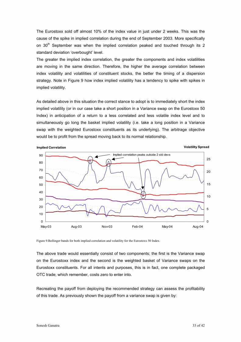
The Eurostoxx sold off almost 10% of the index value in just under 2 weeks. This was the

cause of the spike in implied correlation during the end of September 2003. More specifically

on 30th September was when the implied correlation peaked and touched through its 2

standard deviation ‘overbought’ level.

The greater the implied index correlation, the greater the components and index volatilities

are moving in the same direction. Therefore, the higher the average correlation between

index volatility and volatilities of constituent stocks, the better the timing of a dispersion

strategy. Note in Figure 9 how index implied volatility has a tendency to spike with spikes in

implied volatility.

As detailed above in this situation the correct stance to adopt is to immediately short the index

implied volatility (or in our case take a short position in a Variance swap on the Eurostoxx 50

Index) in anticipation of a return to a less correlated and less volatile index level and to

simultaneously go long the basket implied volatility (i.e. take a long position in a Variance

swap with the weighted Eurostoxx constituents as its underlying). The arbitrage objective

would be to profit from the spread moving back to its normal relationship.

Figure 9.Bollinger bands for both implied correlation and volatility for the Eurostoxx 50 Index.

The above trade would essentially consist of two components; the first is the Variance swap

on the Eurostoxx index and the second is the weighted basket of Variance swaps on the

Eurostoxx constituents. For all intents and purposes, this is in fact, one complete packaged

OTC trade; which remember, costs zero to enter into.

Recreating the payoff from deploying the recommended strategy can assess the profitability

of this trade. As previously shown the payoff from a variance swap is given by:

0

10

20

30

40

50

60

70

80

90

May-03 Aug-03 Nov-03 Feb-04 May-04 Aug-04

Implied Correlation

0

5

10

15

20

25

Volatility Spread

Implied correlation peaks outside 2 std devs


Notional )level Reference - y volatilit(Realized Payoff 22 ×=

where, 2

1

0

12 ln1y volatilitRealized ∑−

=

+

==

n

i i

i

SS

nVar (24)

Note that as the variance swap approaches maturity, exposure to implied volatility declines

and exposure to realized volatility increases, until at maturity the payout depends purely on

realized volatility.

The reference level of the variance swap can be inferred by setting the value of the variance

swap to zero at inception. The variance swap rate represents the risk-neutral expected value

of the realized return variance and reflects not just at-the-money implied volatility but also the

price of other strikes, as described by the volatility skew.

It is worth noting that in the equity options market equity variance swaps trade at a premium

to the at-the-money implied volatility. This is as a result of the put skew inherent in the market.

The Exotic Options trading desk at Dresdner Kleinwort Wasserstein were kind enough to

allow me to use their proprietary variance swap pricing model to infer the strike levels in both

the Eurostoxx Index and its constituent members for the times the trades were entered into.

The limitation of their pricing system meant that we had to make a dividend assumption. The

assumption being that current dividend levels are assumed to be the same as dividend levels

in the past. The impact of this assumption is not deemed a major shortcoming in the

implementation since dividend levels have not changed drastically over the period being

tested. It is anticipated that this will not have insignificant impact on any findings.

Additional inputs into the model include the volatility surface, at the time of inception of the

trade for Eurostoxx index and all its constituent members, since the replicating portfolio

consists of a portfolio of options across all different strikes. More specifically we are interested

in the volatility smile across all strikes for a 3-month term to maturity as we are utilizing a

corresponding 3 month implied correlation measure for our strategy. We perceive that using

an implied correlation measure of less than 3-months would prove too sensitive a measure to

use as a trading indicator and would potentially lead to too many false trading entry points

and may contain too much ‘noise’. A 3 month indicator is generally perceived as being fairly

stable. The 3 month volatility smile for the Eurostoxx and corresponding members were

retrieved from DRKW’s ‘SPOTS’ database. Similarly, we were able to extract the Euribor

interest rates (3 month interest rate Euribor) from the same source.

The historic index constituents and their corresponding market capitalized weights were found

to be directly available from the official ‘Stoxx’ website (www.stoxx.com).

http://www.stoxx.com/


The realized variance was calculated using daily closing price data obtained from Bloomberg.

Another issue that we needed to consider was the size of the long volatility position to the size

of the short volatility position. Academic research has shown that there is no ideal or perfect

ratio. It is at the discretion of the investor as to whether they wish to introduce a vega bias to

the trade. For our purposes, however, we will initiate the trade with zero vega bias.

To implement a zero vega bias we require the sensitivity of the index variance swap to

change in volatility of stock i . The sensitivity to stock i is given by

i

B

Bi

VVσσ

σσ ∂∂

∂∂

=∂∂

(25)

but from before we know that,

∑ ∑∑= = +=

+=n

i

n

i

n

ijjijiavgiiB

1 1 1

22 2 σσωωρσωσ (26)

thus,

B

n

ijj

jjiavgii

B

n

jjjiavgii

i

B

σ

σωωρσω

σ

σωωρσω

σσ

∑∑≠=

=

+

=+

=∂∂ 1

2

1

2 22

21

(27)

For every unit of the Index Variance swap entered into, we must trade in the opposite

direction, the corresponding ratio of the Single stock basket variance swap to initiate a vega-

neutral portfolio. These have been calculated and tabulated below for each of the three

instances when implied correlation breached its two standard deviation Bollinger band during

our period of empirical analysis.

Breach Case Breach Date Vega Ratio Case A 30 Sep 2003 0.76 Case B 25 Nov 2003 0.75 Case C 09 Mar 2004 0.70

3.4 Presentation of results

Based on the trading strategy presented we were able to compute the profitability of

the dispersion trades using the methodology and assumptions illustrated above. The Variance

swap was assumed to be entered into and held for the full 3-month term to maturity at which

time any profit and loss was realized.


Case Implied Correlation Strategy Profit/Loss

A Peak Short Index Vol/Long Basket Vol 1.19 B Peak Short Index Vol/Long Basket Vol 1.51 C Trough Long Index Vol/Short Basket Vol 0.08

The profit and loss indicates the return from the trade in volatility points. Note that the above

analysis assumes a 1.5% bid-offer spread for each transaction. Other transaction costs are

assumed negligible.

The results generated seem to indicate modest profitability in each case. All trades spawned

a humble profit. The cases where Implied correlation peaked appear to be more profitable

than the case where implied correlation troughed. Intuitively this is what an investor would

expect, since an upspike in implied correlation typically occurs when the market experiences

a significant sell-off due to a market event/uncertainty, this is rationally when the implied

volatilities move together. The mean reversion tendencies of the implied correlation tend to be

stronger in these instances than in the case when correlation is low as a result of market

conditions in which asset prices are growing gradually and progressively.

Given the fact that the trading strategy was successful for the trades considered, it would

have been interesting to explore a larger number of trades to investigate whether they would

also have been consistent with the above findings. The prime focus of this thesis was to

illustrate the how to employ variance swaps in dispersion trading arbitrage. A backtest of a

larger number of trades can therefore be left as an area for further analysis.


CONCLUSIONS


The thesis discussed the calculation and implementation of implied correlation as a

valuation method for the implied volatility of a basket or index option implied volatility. We

have suggested how a trader may find a practical application for this useful and relatively

simple tool.

We suggest that implied correlation for dispersion trading is an extremely useful and

potentially profitable vehicle for tracing any disparity/inefficiency in the market.

More importantly, we have introduced the concept of using Variance swaps in the execution

of correlation dispersion trades. This is in contrast the more traditional method of trading

strangles on index and basket options. Variance swaps require no delta hedging and are

therefore less operationally intensive than standard delta-hedged option strategies. This

method of trading should not be underestimated and receive merits for its attractive qualities.

Furthermore, we were able to show how Bollinger bands can be used as an indicator to

identify potential trading opportunities. However, due to the limitations on historical data

availability, the trading rule could not be tested thoroughly enough for the level of significance

of the trading profits. However, one anticipates that the dispersion strategy outlined has been

designed to generate a consistent return with a low correlation to the underlying market in a

variety of market regimes.

This thesis indicates that using Variance swaps in correlation dispersion trading strategies

can be profitable, but a backtest on a larger number of trades is recommended.

Dispersion trading continues to evolve and be refined. One potential future development that

investors expect to see is the OTC commoditization of implied correlation, so that the investor

could simply take a position on the degree of implied correlation in the form of a swap. Much

in the same way as the variance swap.

This would allow the end user to gain the benefit of trading implied correlation without the

computational or trading difficulties, the investment bank or swap counterparty would then

have to hedge this correlation risk, much as they would that of a conventional OTC basket

trade or even as they would a variance swap as the payoff would be similar.


References

Alexander, C. (2001) “Market Models: A Guide to Financial Data Analysis.” John Wiley &

Sons

Avellaneda M. (2002) “Empirical Aspects of Dispersion Trading in U.S. Equity Markets.” Petit

Dejeuner De la Finance

Bernhard G and Daiss M. (2003) “Nonlinear Index Arbitrage.” Quantitative Strategies

Research Notes, Equity Derivatives Research, Dresdner Kleinwort Wasserstein Presentation

January 2003

Canina, L. and S. Figlewski (1993) “The Informational Content of Implied Volatility.” Review of

Financial Studies, Volume 6, No 3, 659-81

Chriss, N. and W Morokoff (1999) “Market risk for volatility and variance swaps.” Risk

October, 55-59

Derman, E., M. Kamal, I. Kani and J. Zou (1996) “Valuing Contracts with Payoffs Based on

Realized Volatility.” Global Derivatives (July) Quarterly Review, Equity Derivatives Research,

Goldman Sachs & Co.

Demeretfi K, E. Derman, M. Kamal, and J. Zou (1999) “More than you ever wanted to know

about volatility swaps” Quantitative Strategies Research Notes, Equity Derivatives Research,

Goldman Sachs & Co.

Hull, J. (2000) “Options, Futures, & Other Derivatives” Prentice Hall International , Fourth

edition

Neuberger, A. (1994) “The Log Contact: A new instrument to hedge volatility” Journal of

Portfolio Management, Winter, 74-80

Petsas, K. and N. Porfiris (2002) “Volatility Analysis and Trading Opportunities in the

FTSE/ASE-20 index options of ADEX” Quantitative Research, Athens Derivatives Exchange

(ADEX)

Reghai A. (2001) “Pricing & Hedging Variance Swaps”

Roelfsema M.R. (2000) “Non-linear Index Arbitrage: Exploiting the Dependencies between

Index and Stock Options.” Delft University Press

Walter, C. and J. Lopez (1997) “Is implied correlation worth calculating? Evidence from foreign exchange options and historical data.” Research Paper #9730, Federal Reserve Bank of New York


Appendix I : Eurostoxx 50 Index and Index Constiutent weights, Spot Prices & 3-month Volatility smile as of 30 Sep 2003

Appendix II : Eurostoxx 50 Index and Index Constiutent weights, Spot Prices & 3-month Volatility smile as of 25 Nov 2003

Ric Weight Ticker Date ClosePrice 70% 80% 90% 100% 110% 120% 130% 140%

TOTF.PA 7.39 FP FP Equity 30/09/2003 129.6 29.38 29.38 28.09 26.12 24.60 23.76 23.49 23.48RD.AS 6.66 RDA NA Equity 30/09/2003 37.71 27.57 27.57 26.71 24.72 22.58 21.15 20.58 20.57NOK1V.HE 5.33 NOK1V FH Equity 30/09/2003 13.22 45.94 45.31 43.30 40.90 39.13 37.84 36.86 36.37TEF.MC 4.00 TEF SM Equity 30/09/2003 10.052 31.99 31.87 30.73 27.92 25.48 23.73 22.85 22.78SIEGn.DE 3.58 SIE GY Equity 30/09/2003 51.14 43.69 42.46 39.59 36.96 34.82 33.11 32.15 31.93BNPP.PA 3.01 BNP FP Equity 30/09/2003 42.1 38.23 38.23 37.65 35.38 32.98 31.26 30.16 29.68SAN.MC 2.92 SAN SM Equity 30/09/2003 7.28 37.09 36.76 35.27 32.60 30.33 28.50 27.20 26.97ENI.MI 2.83 ENI IM Equity 30/09/2003 13.119 24.99 24.95 23.70 21.62 20.02 19.28 19.15 19.14AVEP.PA 2.59 AVE FP Equity 30/09/2003 44.55 37.55 36.98 35.21 32.75 30.80 29.33 28.36 27.96DBKGn.DE 2.56 DBK GY Equity 30/09/2003 52.25 42.46 41.42 38.50 35.37 32.71 30.53 29.32 28.99DTEGn.DE 2.52 DTE GY Equity 30/09/2003 12.44 32.57 32.41 30.84 28.86 27.12 25.78 25.27 25.19UNc.AS 2.43 UNC NA Equity 30/09/2003 50.5 26.54 26.46 24.67 22.07 19.85 18.95 18.82 18.82ING.AS 2.39 INGA NA Equity 30/09/2003 15.73 46.40 45.96 43.94 40.66 37.86 35.64 34.57 34.31BBVA.MC 2.38 BBVA SM Equity 30/09/2003 8.86 34.91 34.87 34.46 32.10 29.82 27.80 26.21 25.40EONG.DE 2.30 EOA GY Equity 30/09/2003 41.9 32.41 32.32 30.99 27.97 24.93 22.56 21.35 21.26SOGN.PA 2.11 GLE FP Equity 30/09/2003 57.2 38.68 38.17 35.95 33.19 31.04 29.49 28.61 28.37PHG.AS 2.09 PHIA NA Equity 30/09/2003 19.46 53.19 51.18 48.10 45.34 43.15 41.48 40.32 39.80DCXGn.DE 2.08 DCX GY Equity 30/09/2003 30.14 46.28 44.81 41.84 38.92 36.48 34.57 33.36 32.95ALVG.DE 2.08 ALV GY Equity 30/09/2003 75.8 51.66 49.28 46.09 43.41 41.28 39.59 38.32 37.75CARR.PA 2.08 CA FP Equity 30/09/2003 43.2 33.64 33.53 32.19 29.70 27.54 25.96 25.07 24.95AAH.AS 2.01 AABA NA Equity 30/09/2003 15.85 35.04 34.72 33.13 30.24 27.48 25.25 23.87 23.60BASF.DE 1.81 BAS GY Equity 30/09/2003 37.7 35.42 35.17 33.50 30.74 28.20 26.07 24.71 24.50GASI.MI 1.80 G IM Equity 30/09/2003 19.38 29.98 29.89 28.43 26.30 24.43 23.20 22.78 22.74AXAF.PA 1.70 CS FP Equity 30/09/2003 14.47 44.89 43.89 41.33 38.29 35.93 34.11 32.73 31.97CRDI.MI 1.64 UC IM Equity 30/09/2003 4.061 24.82 24.60 22.97 20.41 18.68 18.44 18.44 18.44TLIT.MI 1.62 TIT IM Equity 30/09/2003 2.118 29.64 29.58 28.48 26.75 25.17 24.02 23.53 23.47SASY.PA 1.61 SAN FP Equity 30/09/2003 52.2 36.58 36.22 34.23 31.47 29.27 27.62 26.66 26.44OREP.PA 1.55 OR FP Equity 30/09/2003 58.65 31.30 31.20 29.51 27.47 25.72 24.38 23.91 23.86FTE.PA 1.52 FTE FP Equity 30/09/2003 19.75 45.39 43.94 40.84 37.70 35.51 34.03 33.11 32.66FOR.AS 1.48 FORA NA Equity 30/09/2003 14.59 39.76 39.22 37.25 34.43 32.05 30.32 29.42 29.34DANO.PA 1.40 BN FP Equity 30/09/2003 65.5 24.30 24.30 24.30 24.30 24.30 24.30 24.30 24.30EAUG.PA 1.37 EX FP Equity 30/09/2003 15.2 51.89 50.05 45.96 42.85 40.64 39.05 37.94 37.19TIM.MI 1.25 TIM IM Equity 30/09/2003 3.993 27.74 27.69 26.73 25.07 23.66 23.05 22.97 22.97AEGN.AS 1.11 AGN NA Equity 30/09/2003 9.99 52.00 51.17 48.62 45.70 43.20 41.21 39.74 38.96REP.MC 1.11 REP SM Equity 30/09/2003 14.11 26.52 26.50 26.15 24.62 22.24 20.38 19.59 19.44LYOE.PA 1.07 SZE FP Equity 30/09/2003 13.63 46.23 44.53 41.41 38.72 36.67 35.10 33.87 32.91BAYG.DE 1.07 BAY GY Equity 30/09/2003 18.55 44.31 43.45 41.07 37.92 35.44 33.39 31.63 30.75ELE.MC 1.06 ELE SM Equity 30/09/2003 13.27 28.55 27.60 25.56 23.32 21.40 19.78 18.44 17.52LVMH.PA 1.06 MC FP Equity 30/09/2003 53.35 35.62 35.26 33.10 30.66 28.75 27.47 26.95 26.86AIRP.PA 1.02 AI FP Equity 30/09/2003 110.27 36.42 36.35 35.16 32.33 29.89 27.89 26.27 25.22CGEP.PA 0.98 CGE FP Equity 30/09/2003 10.17 53.73 52.88 49.83 47.11 45.04 43.45 42.29 41.77IBE.MC 0.94 IBE SM Equity 30/09/2003 14.45 21.70 21.69 21.25 19.87 18.36 17.56 17.38 17.38SGOB.PA 0.92 SGO FP Equity 30/09/2003 31.57 37.74 37.46 36.15 33.76 31.68 29.95 28.61 27.88MUVGn.DE 0.92 MUV2 GY Equity 30/09/2003 81.139 51.00 49.91 47.51 44.99 43.01 41.40 40.07 39.03ENEI.MI 0.87 ENEL IM Equity 30/09/2003 5.34 24.77 24.75 24.11 22.55 20.89 19.80 19.33 19.30SPI.MI 0.86 SPI IM Equity 30/09/2003 8.559 39.16 38.24 35.19 32.80 31.03 29.85 29.66 29.64LAFP.PA 0.78 LG FP Equity 30/09/2003 55.65 39.35 38.62 36.06 33.55 31.50 29.78 28.86 28.66RWEG.DE 0.78 RWE GY Equity 30/09/2003 22.84 31.98 31.88 30.77 28.94 27.20 25.75 24.90 24.76VOWG.DE 0.72 VOW GY Equity 30/09/2003 38.59 49.78 47.01 43.24 40.25 37.86 35.81 34.43 34.09AHLN.AS 0.64 AHLN NA Equity 30/09/2003 6.927 72.80 69.61 64.66 59.43 55.28 52.10 49.51 47.43

50% 60% 70% 80% 90% 100% 110% 120%.STOXX50E SX5E Index 30/09/2003 2395.87 51.20 46.69 42.03 37.37 32.78 28.30 24.16 21.40

130% 140% 150% 160% 170% 180% 190% 200%19.89 19.34 19.58 20.53 21.93 23.60 25.20 26.60

Volatility Smile (% of ATM strike)


Appendix III : Eurostoxx 50 Index and Index Constiutent weights, Spot Prices & 3-month Volatility smile as of 09 Mar2004


TOTF.PA 6.94 FP FP Equity 09/03/2004 149.9 23.00 22.95 21.20 19.08 17.91 17.75 17.75 17.75RD.AS 5.77 RDA NA Equity 09/03/2004 40.35 20.07 19.99 18.81 16.71 15.55 15.49 15.49 15.49NOK1V.HE 5.72 NOK1V FH Equity 09/03/2004 18.22 35.50 33.11 30.89 29.59 29.09 29.01 29.01 29.01TEF.MC 4.13 TEF SM Equity 09/03/2004 13.11 25.00 23.82 22.00 20.65 20.08 20.07 20.07 20.07SIEGn.DE 3.60 SIE GY Equity 09/03/2004 62.87 33.51 33.16 30.63 28.07 26.00 24.43 23.94 23.88SAN.MC 3.10 SAN SM Equity 09/03/2004 9.17 28.20 28.02 25.87 23.28 21.22 20.06 19.81 19.81BNPP.PA 3.03 BNP FP Equity 09/03/2004 49.78 28.64 28.08 25.62 22.96 21.07 20.36 20.32 20.32ENI.MI 3.02 ENI IM Equity 09/03/2004 16.3 20.10 19.83 18.41 16.31 15.29 15.12 15.12 15.12DBKGn.DE 3.01 DBK GY Equity 09/03/2004 72.47 35.03 33.86 31.27 28.70 27.51 27.30 27.30 27.30AVEP.PA 2.82 AVE FP Equity 09/03/2004 62.8 24.07 24.07 22.67 20.55 19.16 18.77 18.76 18.76DTEGn.DE 2.62 DTE GY Equity 09/03/2004 15.92 29.58 29.54 28.26 26.24 24.32 22.89 22.30 22.25ING.AS 2.52 INGA NA Equity 09/03/2004 19.61 31.83 31.48 29.35 26.50 24.35 23.04 22.57 22.56BBVA.MC 2.52 BBVA SM Equity 09/03/2004 11.12 29.55 28.95 26.39 23.99 22.30 21.46 21.40 21.40EONG DE 2 31 EOA GY E it 09/03/2004 55 73 26 09 26 01 23 46 21 15 19 60 19 32 19 31 19 31

Volatility Smile (% of ATM strike)


TOTF.PA 6.97 FP FP Equity 134.5 25.27 25.27 24.29 22.39 21.04 20.60 20.55 20.54RD.AS 6.01 RDA NA Equity 25/11/2003 37.85 23.36 23.36 22.82 21.14 19.04 17.82 17.52 17.51NOK1V.HE 5.49 NOK1V FH Equity 25/11/2003 15.08 39.41 37.98 35.65 33.78 32.43 31.62 31.32 31.27TEF.MC 3.86 TEF SM Equity 25/11/2003 10.72 25.54 25.54 24.29 22.04 20.24 19.42 19.28 19.28SIEGn.DE 3.86 SIE GY Equity 25/11/2003 60.87 36.95 34.82 31.94 29.50 27.71 27.05 26.99 26.99SAN.MC 3.16 SAN SM Equity 25/11/2003 8.63 31.42 29.60 26.76 24.39 23.29 23.16 23.16 23.16BNPP.PA 3.05 BNP FP Equity 25/11/2003 46.31 32.06 31.44 29.41 26.91 25.29 24.67 24.50 24.50ENI.MI 2.78 ENI IM Equity 25/11/2003 14.097 21.57 21.09 19.42 17.56 16.64 16.47 16.47 16.47DBKGn.DE 2.58 DBK GY Equity 25/11/2003 56.71 36.80 35.36 32.03 28.98 26.77 25.66 25.44 25.44AVEP.PA 2.54 AVE FP Equity 25/11/2003 48.24 31.01 30.63 28.75 26.31 24.68 24.10 23.97 23.97DTEGn.DE 2.54 DTE GY Equity 25/11/2003 13.65 28.83 27.72 25.72 23.88 22.52 22.03 21.99 21.99ING.AS 2.46 INGA NA Equity 25/11/2003 17.73 42.19 39.45 35.37 32.10 29.58 27.86 27.19 27.10BBVA.MC 2.44 BBVA SM Equity 25/11/2003 9.99 30.10 29.29 27.04 24.65 22.79 21.88 21.74 21.74EONG.DE 2.36 EOA GY Equity 25/11/2003 46.45 27.72 27.57 25.60 23.18 21.41 20.57 20.56 20.56ALVG.DE 2.33 ALV GY Equity 25/11/2003 91 42.55 41.04 37.96 35.60 33.82 32.54 31.93 31.90PHG.AS 2.31 PHIA NA Equity 25/11/2003 23.75 42.96 40.62 37.71 35.38 33.56 32.48 32.07 32.00SOGN.PA 2.23 GLE FP Equity 25/11/2003 66.6 35.91 32.95 29.95 27.95 26.94 26.65 26.61 26.61UNc.AS 2.18 UNC NA Equity 25/11/2003 51 22.92 22.92 21.93 19.35 17.05 16.18 16.06 16.06AAH.AS 2.11 AABA NA Equity 25/11/2003 18.14 32.94 30.95 27.26 23.86 22.03 21.57 21.54 21.54DCXGn.DE 1.99 DCX GY Equity 25/11/2003 32.03 37.28 36.53 33.81 30.97 28.78 27.47 26.98 26.91CARR.PA 1.96 CA FP Equity 25/11/2003 45.2 31.40 30.58 28.57 26.33 24.84 24.24 24.07 24.05BASF.DE 1.80 BAS GY Equity 25/11/2003 41.46 32.26 31.04 28.45 25.95 23.93 22.79 22.52 22.52GASI.MI 1.75 G IM Equity 25/11/2003 20.74 23.51 23.38 21.91 19.73 18.29 17.80 17.79 17.79AXAF.PA 1.70 CS FP Equity 25/11/2003 15.95 40.03 37.89 34.86 31.97 29.80 28.49 27.82 27.62TLIT.MI 1.68 TIT IM Equity 25/11/2003 2.388 28.66 27.51 25.42 23.71 22.86 22.70 22.70 22.70SASY.PA 1.58 SAN FP Equity 25/11/2003 56.85 32.53 30.61 27.69 25.34 24.15 23.82 23.82 23.82EAUG.PA 1.57 EX FP Equity 25/11/2003 19.29 38.83 35.44 32.81 31.04 30.07 29.74 29.68 29.68CRDI.MI 1.53 UC IM Equity 25/11/2003 4.203 24.98 24.18 21.98 19.69 18.23 17.79 17.77 17.77FTE.PA 1.51 FTE FP Equity 25/11/2003 21.4 37.18 35.71 32.77 29.94 28.14 27.37 27.13 27.11OREP.PA 1.48 OR FP Equity 25/11/2003 62.45 29.63 28.41 26.08 23.86 22.58 22.17 22.10 22.10FOR.AS 1.44 FORA NA Equity 25/11/2003 15.6 31.08 30.58 28.51 25.63 23.48 22.61 22.41 22.41DANO.PA 1.26 BN FP Equity 25/11/2003 64.75 20.36 20.36 20.36 20.36 20.36 20.36 20.36 20.36TIM.MI 1.22 TIM IM Equity 25/11/2003 4.301 23.26 23.06 21.79 20.11 19.25 19.03 19.02 19.02MUVGn.DE 1.19 MUV2 GY Equity 25/11/2003 94.91 43.91 42.67 40.09 37.57 35.58 34.06 33.09 32.69BAYG.DE 1.18 BAY GY Equity 25/11/2003 22.46 37.29 36.43 34.03 31.16 29.05 28.06 27.64 27.63AEGN.AS 1.12 AGN NA Equity 25/11/2003 11.14 47.42 44.48 40.39 37.08 34.50 32.55 31.54 31.17REP.MC 1.04 REP SM Equity 25/11/2003 14.64 24.68 24.67 23.60 21.70 20.11 19.40 19.26 19.26LVMH.PA 1.03 MC FP Equity 25/11/2003 57.6 34.57 32.67 29.84 27.24 25.70 25.15 25.04 25.04LYOE.PA 1.03 SZE FP Equity 25/11/2003 14.14 31.75 30.29 27.88 25.55 24.01 23.26 22.96 22.94AIRP.PA 1.02 AI FP Equity 25/11/2003 121.82 36.09 34.20 31.53 29.19 27.30 25.78 24.75 24.31ELE.MC 1.00 ELE SM Equity 25/11/2003 13.65 24.66 24.62 23.07 20.64 18.65 17.94 17.89 17.89SGOB.PA 0.99 SGO FP Equity 25/11/2003 36.36 37.24 35.45 32.82 30.69 29.24 28.47 28.19 28.14SPI.MI 0.98 SPI IM Equity 25/11/2003 10.644 33.29 30.91 28.27 26.45 25.49 25.13 25.11 25.11CGEP.PA 0.95 CGE FP Equity 25/11/2003 10.87 49.76 47.79 44.89 42.34 40.43 39.07 38.36 37.96IBE.MC 0.85 IBE SM Equity 25/11/2003 14.4 19.68 19.68 18.92 17.26 15.92 15.56 15.54 15.54LAFP.PA 0.85 LG FP Equity 25/11/2003 65.15 35.81 32.75 30.21 28.19 26.90 26.55 26.52 26.52RWEG.DE 0.83 RWE GY Equity 25/11/2003 26.41 29.38 29.13 27.21 25.09 23.47 22.58 22.55 22.55ENEI.MI 0.78 ENEL IM Equity 25/11/2003 5.264 20.83 20.76 19.85 18.08 16.99 16.70 16.70 16.70AHLN.AS 0.71 AHLN NA Equity 25/11/2003 6.995 53.87 53.35 51.69 48.92 45.71 43.11 40.96 39.16VOWG.DE 0.70 VOW GY Equity 25/11/2003 43.08 37.06 36.44 34.47 31.67 29.08 27.32 26.44 26.15SAPG.DE SAP GY Equity 25/11/2003 129.45 43.82 41.85 38.87 36.44 34.59 33.34 32.79 32.67

50% 60% 70% 80% 90% 100% 110% 120%.STOXX50E SX5E Index 25/11/2003 2625.31 40.65 40.64 38.32 32.19 26.58 21.61 18.23 16.83

130% 140% 150% 160% 170% 180% 190% 200%16.62 16.62 16.62 16.62 16.62 16.62 16.62 16.62

Volatiliy Smile (% of ATM Strike)


Appendix IV : Eurostoxxx 50 Index and Index constituent variance swap strike levels

Case A 30-Sep-03 Case B 25-Nov-03 Case C 09-Mar-04

RIC Security Implied Strike Vol RIC Security Implied Strike Vol RIC Security Implied Strike Vol% % %

TEF.MC TELEFONICA 28.27 TEF.MC TELEFONICA 22.47 TEF.MC TELEFONICA 21.03RD.AS ROYAL DUTCH PETROLEUM 24.28 RD.AS ROYAL DUTCH PETROLEUM 20.65 RD.AS ROYAL DUTCH PETROLEUM 16.77ING.AS ING GROEP 40.51 ING.AS ING GROEP 33.00 ING.AS ING GROEP 26.63VOWG.DE VOLKSWAGEN 41.00 VOWG.DE VOLKSWAGEN 31.55 VOWG.DE VOLKSWAGEN 28.54MUVGn.DE MUENCHENER RUECKVER R 44.96 MUVGn.DE MUENCHENER RUECKVER R 37.72 MUVGn.DE MUENCHENER RUECKVER R 29.67AIRP.PA AIR LIQUIDE 31.97 AIRP.PA AIR LIQUIDE 29.35 AIRP.PA AIR LIQUIDE 24.28AHLN.AS AHOLD 61.14 AHLN.AS AHOLD 47.91 AHLN.AS AHOLD 38.69REP.MC REPSOL YPF 23.84 REP.MC REPSOL YPF 21.52 REP.MC REPSOL YPF 17.95RWEG.DE RWE 28.51 RWEG.DE RWE 25.08 RWEG.DE RWE 26.51SGOB.PA SAINT GOBAIN 33.37 SGOB.PA SAINT GOBAIN 31.01 SGOB.PA SAINT GOBAIN 26.04BBVA.MC BCO BILBAO VIZCAYA ARGENT 31.65 BBVA.MC BCO BILBAO VIZCAYA ARGENT 24.98 BBVA.MC BCO BILBAO VIZCAYA ARGENT 24.39BNPP.PA BNP 34.62 BNPP.PA BNP 27.12 BNPP.PA BNP 23.20BAYG.DE BAYER 37.97 BAYG.DE BAYER 31.45 BAYG.DE BAYER 28.43ENEI.MI ENEL 22.13 ENEI.MI ENEL 18.02 ENEI.MI ENEL 15.00

msc mathematical trading &...

Documents