ms3b/mscmcf l´evy processes and financewinkel/ms3b10.pdf · gales and financial mathematics would...
TRANSCRIPT

MS3b/MScMCFLevy Processes and Finance
Matthias WinkelDepartment of Statistics
University of Oxford
HT 2010


MS3b (and MScMCF)Levy Processes and Finance
Matthias Winkel – 16 lectures HT 2010
Prerequisites
Part A Probability is a prerequisite. BS3a/OBS3a Applied Probability or B10 Martin-gales and Financial Mathematics would be useful, but are by no means essential; somematerial from these courses will be reviewed without proof.
Aims
Levy processes form a central class of stochastic processes, contain both Brownian motionand the Poisson process, and are prototypes of Markov processes and semimartingales.Like Brownian motion, they are used in a multitude of applications ranging from biologyand physics to insurance and finance. Like the Poisson process, they allow to modelabrupt moves by jumps, which is an important feature for many applications. In the lastten years Levy processes have seen a hugely increased attention as is reflected on theacademic side by a number of excellent graduate texts and on the industrial side realisingthat they provide versatile stochastic models of financial markets. This continues tostimulate further research in both theoretical and applied directions. This course willgive a solid introduction to some of the theory of Levy processes as needed for financialand other applications.
Synopsis
Review of (compound) Poisson processes, Brownian motion (informal), Markov property.Connection with random walks, [Donsker’s theorem], Poisson limit theorem. SpatialPoisson processes, construction of Levy processes.
Special cases of increasing Levy processes (subordinators) and processes with onlypositive jumps. Subordination. Examples and applications. Financial models drivenby Levy processes. Stochastic volatility. Level passage problems. Applications: optionpricing, insurance ruin, dams.
Simulation: via increments, via simulation of jumps, via subordination. Applications:option pricing, branching processes.
Reading
• J.F.C. Kingman: Poisson processes. Oxford University Press (1993), Ch.1-5, 8
• A.E. Kyprianou: Introductory lectures on fluctuations of Levy processes with Ap-plications. Springer (2006), Ch. 1-3, 8-9
• W. Schoutens: Levy processes in finance: pricing financial derivatives. Wiley (2003)
Further reading
• J. Bertoin: Levy processes. Cambridge University Press (1996), Sect. 0.1-0.6, I.1,III.1-2, VII.1
• K. Sato: Levy processes and infinite divisibility. Cambridge University Press (1999),Ch. 1-2, 4, 6, 9


Contents
1 Introduction 1
1.1 Definition of Levy processes . . . . . . . . . . . . . . . . . . . . . . . . . 1
1.2 First main example: Poisson process . . . . . . . . . . . . . . . . . . . . 2
1.3 Second main example: Brownian motion . . . . . . . . . . . . . . . . . . 3
1.4 Markov property . . . . . . . . . . . . . . . . . . . . . . . . . . . . . . . 4
1.5 Some applications . . . . . . . . . . . . . . . . . . . . . . . . . . . . . . . 4
2 Levy processes and random walks 5
2.1 Increments of random walks and Levy processes . . . . . . . . . . . . . . 5
2.2 Central Limit Theorem and Donsker’s theorem . . . . . . . . . . . . . . . 6
2.3 Poisson limit theorem . . . . . . . . . . . . . . . . . . . . . . . . . . . . . 8
2.4 Generalisations . . . . . . . . . . . . . . . . . . . . . . . . . . . . . . . . 8
3 Spatial Poisson processes 9
3.1 Motivation from the study of Levy processes . . . . . . . . . . . . . . . . 9
3.2 Poisson counting measures . . . . . . . . . . . . . . . . . . . . . . . . . . 10
3.3 Poisson point processes . . . . . . . . . . . . . . . . . . . . . . . . . . . . 12
4 Spatial Poisson processes II 13
4.1 Series and increasing limits of random variables . . . . . . . . . . . . . . 13
4.2 Construction of spatial Poisson processes . . . . . . . . . . . . . . . . . . 14
4.3 Sums over Poisson point processes . . . . . . . . . . . . . . . . . . . . . . 15
4.4 Martingales (from B10a) . . . . . . . . . . . . . . . . . . . . . . . . . . . 16
5 The characteristics of subordinators 17
5.1 Subordinators and the Levy-Khintchine formula . . . . . . . . . . . . . . 17
5.2 Examples . . . . . . . . . . . . . . . . . . . . . . . . . . . . . . . . . . . 19
5.3 Aside: nonnegative Levy processes . . . . . . . . . . . . . . . . . . . . . 19
5.4 Applications . . . . . . . . . . . . . . . . . . . . . . . . . . . . . . . . . . 20
6 Levy processes with no negative jumps 21
6.1 Bounded and unbounded variation . . . . . . . . . . . . . . . . . . . . . 21
6.2 Martingales (from B10a) . . . . . . . . . . . . . . . . . . . . . . . . . . . 22
6.3 Compensation . . . . . . . . . . . . . . . . . . . . . . . . . . . . . . . . . 23
v

vi Contents
7 General Levy processes and simulation 25
7.1 Construction of Levy processes . . . . . . . . . . . . . . . . . . . . . . . 25
7.2 Simulation via embedded random walks . . . . . . . . . . . . . . . . . . . 27
7.3 R code – not examinable . . . . . . . . . . . . . . . . . . . . . . . . . . . 29
8 Simulation II 31
8.1 Simulation via truncated Poisson point processes . . . . . . . . . . . . . 31
8.2 Generating specific distributions . . . . . . . . . . . . . . . . . . . . . . . 34
8.3 R code – not examinable . . . . . . . . . . . . . . . . . . . . . . . . . . . 36
9 Simulation III 37
9.1 Applications of the rejection method . . . . . . . . . . . . . . . . . . . . 37
9.2 “Errors increase in sums of approximated terms.” . . . . . . . . . . . . . 38
9.3 Approximation of small jumps by Brownian motion . . . . . . . . . . . . 40
9.4 Appendix: Consolidation on Poisson point processes . . . . . . . . . . . . 41
9.5 Appendix: Consolidation on the compensation of jumps . . . . . . . . . . 41
10 Levy markets and incompleteness 43
10.1 Arbitrage-free pricing (from B10b) . . . . . . . . . . . . . . . . . . . . . 43
10.2 Introduction to Levy markets . . . . . . . . . . . . . . . . . . . . . . . . 45
10.3 Incomplete discrete financial markets . . . . . . . . . . . . . . . . . . . . 46
11 Levy markets and time-changes 49
11.1 Incompleteness and martingale probabilities in Levy markets . . . . . . . 49
11.2 Option pricing by simulation . . . . . . . . . . . . . . . . . . . . . . . . . 50
11.3 Time changes . . . . . . . . . . . . . . . . . . . . . . . . . . . . . . . . . 50
11.4 Quadratic variation of time-changed Brownian motion . . . . . . . . . . . 52
12 Subordination and stochastic volatility 55
12.1 Bochner’s subordination . . . . . . . . . . . . . . . . . . . . . . . . . . . 55
12.2 Ornstein-Uhlenbeck processes . . . . . . . . . . . . . . . . . . . . . . . . 57
12.3 Simulation by subordination . . . . . . . . . . . . . . . . . . . . . . . . . 58
13 Level passage problems 59
13.1 The strong Markov property . . . . . . . . . . . . . . . . . . . . . . . . . 59
13.2 The supremum process . . . . . . . . . . . . . . . . . . . . . . . . . . . . 60
13.3 Levy processes with no positive jumps . . . . . . . . . . . . . . . . . . . 61
13.4 Application: insurance ruin . . . . . . . . . . . . . . . . . . . . . . . . . 62
14 Ladder times and storage models 63
14.1 Case 1: No positive jumps . . . . . . . . . . . . . . . . . . . . . . . . . . 63
14.2 Case 2: Union of intervals as ladder time set . . . . . . . . . . . . . . . . 65
14.3 Case 3: Discrete ladder time set . . . . . . . . . . . . . . . . . . . . . . . 66
14.4 Case 4: non-discrete ladder time set and positive jumps . . . . . . . . . . 66

Contents vii
15 Branching processes 6715.1 Galton-Watson processes . . . . . . . . . . . . . . . . . . . . . . . . . . . 6715.2 Continuous-time Galton-Watson processes . . . . . . . . . . . . . . . . . 6815.3 Continuous-state branching processes . . . . . . . . . . . . . . . . . . . . 70
16 The two-sided exit problem 7116.1 The two-sided exit problem for Levy processes with no negative jumps . 7116.2 The two-sided exit problem for Brownian motion . . . . . . . . . . . . . 7216.3 Appendix: Donsker’s Theorem revisited . . . . . . . . . . . . . . . . . . . 73
A Assignments IA.1 Infinite divisibility and limits of random walks . . . . . . . . . . . . . . . IIIA.2 Poisson counting measures . . . . . . . . . . . . . . . . . . . . . . . . . . VA.3 Construction of Levy processes . . . . . . . . . . . . . . . . . . . . . . . VIIA.4 Simulation . . . . . . . . . . . . . . . . . . . . . . . . . . . . . . . . . . . IXA.5 Financial models . . . . . . . . . . . . . . . . . . . . . . . . . . . . . . . XIA.6 Time change . . . . . . . . . . . . . . . . . . . . . . . . . . . . . . . . . . XIIIA.7 Subordination and level passage events . . . . . . . . . . . . . . . . . . . XV
B Solutions XVIIB.1 Infinite divisibility and limits of random walks . . . . . . . . . . . . . . . XVIIB.2 Poisson counting measures . . . . . . . . . . . . . . . . . . . . . . . . . . XXIIB.3 Construction of Levy processes . . . . . . . . . . . . . . . . . . . . . . . XXVIB.4 Simulation . . . . . . . . . . . . . . . . . . . . . . . . . . . . . . . . . . . XXXIB.5 Financial models . . . . . . . . . . . . . . . . . . . . . . . . . . . . . . . XXXVB.6 Time change . . . . . . . . . . . . . . . . . . . . . . . . . . . . . . . . . . XXXIXB.7 Subordination and level passage events . . . . . . . . . . . . . . . . . . . XLIII

Lecture 1
Introduction
Reading: Kyprianou Chapter 1Further reading: Sato Chapter 1, Schoutens Sections 5.1 and 5.3
In this lecture we give the general definition of a Levy process, study some examples ofLevy processes and indicate some of their applications. By doing so, we will review someresults from BS3a Applied Probability and B10 Martingales and Financial Mathematics.
1.1 Definition of Levy processes
Stochastic processes are collections of random variables Xt, t ≥ 0 (meaning t ∈ [0,∞)as opposed to n ≥ 0 by which means n ∈ N = 0, 1, 2, . . .). For us, all Xt, t ≥ 0, takevalues in a common state space, which we will choose specifically as R (or [0,∞) or Rd
for some d ≥ 2). We can think of Xt as the position of a particle at time t, changing ast varies. It is natural to suppose that the particle moves continuously in the sense thatt 7→ Xt is continuous (with probability 1), or that it has jumps for some t ≥ 0:
∆Xt = Xt+ −Xt− = limε↓0
Xt+ε − limε↓0
Xt−ε.
We will usually suppose that these limits exist for all t ≥ 0 and that in fact Xt+ = Xt,i.e. that t 7→ Xt is right-continuous with left limits Xt− for all t ≥ 0 almost surely. Thepath t 7→ Xt can then be viewed as a random right-continuous function.
Definition 1 (Levy process) A real-valued (or Rd-valued) stochastic process X =(Xt)t≥0 is called a Levy process if
(i) the random variables Xt0 , Xt1 −Xt0 , . . . , Xtn −Xtn−1 are independent for all n ≥ 1and 0 ≤ t0 < t1 < . . . < tn(independent increments),
(ii) Xt+s −Xt has the same distribution as Xs for all s, t ≥ 0 (stationary increments),
(iii) the paths t 7→ Xt are right-continuous with left limits (with probability 1).
It is implicit in (ii) that P(X0 = 0) = 1 (choose s = 0).
1

2 Lecture Notes – MS3b Levy Processes and Finance – Oxford HT 2010
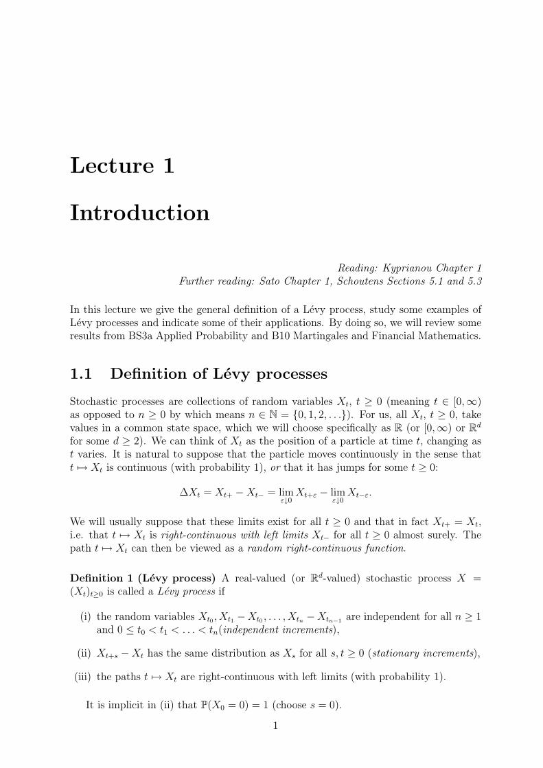
Figure 1.1: Variance Gamma process and a Levy process with no positive jumps
Here the independence of n random variables is understood in the following sense:
Definition 2 (Independence) Let Y (j) be an Rdj -valued random variable for j =1, . . . , n. The random variables Y (1), . . . , Y (n) are called independent if, for all (Borelmeasurable) C(j) ⊂ Rdj
P(Y (1) ∈ C(1), . . . , Y (n) ∈ C(n)) = P(Y (1) ∈ C(1)) . . .P(Y (n) ∈ C(n)). (1)
An infinite collection (Y (j))j∈J is called independent if Y (j1), . . . , Y (jn) are independent for
every finite subcollection. Infinite-dimensional random variables (Y(1)i )i∈I1, . . . , (Y
(n)i )i∈In
are called independent if (Y(1)i )i∈F1, . . . , (Y
(n)i )i∈Fn are independent for all finite Fj ⊂ Ij .
It is sufficient to check (1) for rectangles of the form C(j) = (a(j)1 , b
(j)1 ] × . . .× (a
(j)dj, b
(j)dj
].
1.2 First main example: Poisson process
Poisson processes are Levy processes. We recall the definition as follows. An N(⊂ R)-valued stochastic process X = (Xt)t≥0 is called a Poisson process with rate λ ∈ (0,∞) ifX satisfies (i)-(iii) and
(iv)Poi P(Xt = k) = (λt)k
k!e−λt, k ≥ 0, t ≥ 0 (Poisson distribution).
The Poisson process is a continuous-time Markov chain. We will see that all Levy pro-cesses have a Markov property. Also recall that Poisson processes have jumps of size 1(spaced by independent exponential random variables Zn = Tn+1−Tn, n ≥ 0, with param-eter λ, i.e. with density λe−λs, s ≥ 0). In particular, t ≥ 0 : ∆Xt 6= 0 = Tn, n ≥ 1and ∆XTn = 1 almost surely (short a.s., i.e. with probability 1). We can define moregeneral Levy processes by putting
Ct =Xt∑
k=1
Yk, t ≥ 0,
for a Poisson process (Xt)t≥0 and independent identically distributed Yk, k ≥ 1. Suchprocesses are called compound Poisson processes. The term “compound” stems from therepresentation Ct = S Xt = SXt for the random walk Sn = Y1 + . . . + Yn. You maythink of Xt as the number of claims up to time t and of Yk as the size of the kth claim.Recall (from BS3a) that its moment generating function, if it exists, is given by
E(expγCt) = expλt(E(eγY1 − 1)).This will be an important building block of a general Levy process.

Lecture 1: Introduction 3
Figure 1.2: Poisson process and Brownian motion
1.3 Second main example: Brownian motion
Brownian motion is a Levy process. We recall (from B10b) the definition as follows. AnR-valued stochastic process X = (Xt)t≥0 is called Brownian motion if X satisfies (i)-(ii)and
(iii)BM the paths t 7→ Xt are continuous almost surely,
(iv)BM P(Xt ≤ x) =∫ x−∞
1√2πt
exp−y2
2t
dy, x ∈ R, t > 0. (Normal distribution).
The paths of Brownian motion are continuous, but turn out to be nowhere differentiable(we will not prove this). They exhibit erratic movements at all scales. This makesBrownian motion an appealing model for stock prices. Brownian motion has the scalingproperty (
√cXt/c)t≥0 ∼ X where “∼” means “has the same distribution as”.
Brownian motion will be the other important building block of a general Levy process.The canonical space for Brownian paths is the space C([0,∞),R) of continuous real-
valued functions f : [0,∞) → R which can be equipped with the topology of locallyuniform convergence, induced by the metric
d(f, g) =∑
k≥1
2−k mindk(f, g), 1, where dk(f, g) = supx∈[0,k]
|f(x) − g(x)|.
This metric topology is complete (Cauchy sequences converge) and separable (has acountable dense subset), two attributes important for the existence and properties oflimits. The bigger space D([0,∞),R) of right-continuous real-valued functions with leftlimits can also be equipped with the topology of locally uniform convergence. The spaceis still complete, but not separable. There is a weaker metric topology, called Skorohod’stopology, that is complete and separable. In the present course we will not developthis and only occasionally use the familiar uniform convergence for (right-continuous)functions f, fn : [0, k] → R, n ≥ 1:
supx∈[0,k]
|fn(x) − f(x)| → 0, as n→ ∞,
which for stochastic processes X,X(n), n ≥ 1, with time range t ∈ [0, T ] takes the form
supt∈[0,T ]
|X(n)t −Xt| → 0, as n→ ∞,
and will be as a convergence in probability or as almost sure convergence (from BS3a orB10a) or as L2-convergence, where Zn → Z in the L2-sense means E(|Zn − Z|2) → 0.

4 Lecture Notes – MS3b Levy Processes and Finance – Oxford HT 2010
1.4 Markov property
The Markov property is a consequence of the independent increments property (and thestationary increments property):
Proposition 3 (Markov property) Let X be a Levy process and t ≥ 0 a fixed time,then the pre-t process (Xr)r≤t is independent of the post-t process (Xt+s−Xt)s≥0, and thepost-t process has the same distribution as X.
Proof: By Definition 2, we need to check the independence of (Xr1, . . . , Xrn) and (Xt+s1−Xt, . . . , Xt+sm −Xt). By property (i) of the Levy process, we have that increments overdisjoint time intervals are independent, in particular the increments
Xr1, Xr2 −Xr1 , . . . , Xrn −Xrn−1 , Xt+s1 −Xt, Xt+s2 −Xt+s1 , . . . , Xt+sm −Xt+sm−1 .
Since functions (here linear transformations from increments to marginals) of independentrandom variables are independent, the proof of independence is complete. Identicaldistribution follows first on the level of single increments from (ii), then by (i) and lineartransformation also for finite-dimensional marginal distributions. 2
1.5 Some applications
Example 4 (Insurance ruin) A compound Poisson process (Zt)t≥0 with positive jumpsizes Ak, k ≥ 1, can be interpreted as a claim process recording the total claim amountincurred before time t. If there is linear premium income at rate r > 0, then also thegain process rt− Zt, t ≥ 0, is a Levy process. For an initial reserve of u > 0, the reserveprocess u+ rt− Zt is a shifted Levy process starting from a non-zero initial value u.
Example 5 (Financial stock prices) Brownian motion (Bt)t≥0 or linear Brownian mo-tion σBt +µt, t ≥ 0, was the first model of stock prices, introduced by Bachelier in 1900.Black, Scholes and Merton studied geometric Brownian motion exp(σBt + µt) in 1973,which is not itself a Levy process but can be studied with similar methods. The EconomicsNobel Prize 1997 was awarded for their work. Several deficiencies of the Black-Scholesmodel have been identified, e.g. the Gaussian density decreases too quickly, no variationof the volatility σ over time, no macroscopic jumps in the price processes. These deficien-cies can be addressed by models based on Levy processes. The Variance gamma modelis a time-changed Brownian motion BTs by an independent increasing jump process, aso-called Gamma Levy process with Ts ∼ Gamma(αs, β). The process BTs is then also aLevy process itself.
Example 6 (Population models) Branching processes are generalisations of birth-and-death processes (see BS3a) where each individual in a population dies after an ex-ponentially distributed lifetime with parameter µ, but gives birth not to single children,but to twins, triplets, quadruplet etc. To simplify, it is assumed that children are onlyborn at the end of a lifetime. The numbers of children are independent and identicallydistributed according to an offspring distribution q on 0, 2, 3, . . .. The population sizeprocess (Zt)t≥0 can jump downwards by 1 or upwards by an integer. It is not a Levyprocess but is closely related to Levy processes and can be studied with similar meth-ods. There are also analogues of processes in [0,∞), so-called continuous-state branchingprocesses that are useful large-population approximations.

Lecture 2
Levy processes and random walks
Reading: Kingman Section 1.1, Grimmett and Stirzaker Section 3.5(4)Further reading: Sato Section 7, Durrett Sections 2.8 and 7.6, Kallenberg Chapter 15
Levy processes are the continuous-time analogues of random walks. In this lecture weexamine this analogy and indicate connections via scaling limits and other limiting results.We begin with a first look at infinite divisibility.
2.1 Increments of random walks and Levy processes
Recall that a random walk is a stochastic process in discrete time
S0 = 0, Sn =
n∑
j=1
Aj, n ≥ 1,
for a family (Aj)j≥1 of independent and identically distributed real-valued (or Rd-valued)random variables. Clearly, random walks have stationary and independent increments.Specifically, the Aj , j ≥ 1, themselves are the increments over single time units. We referto Sn+m − Sn as an increment over m time units, m ≥ 1.
While every distribution may be chosen for Aj , increments over m time units are sumsofm independent and identically distributed random variables, and not every distributionhas this property. This is not a deep observation, but it becomes important when movingto Levy processes. In fact, the increment distribution of Levy processes is restricted: anyincrement Xt+s −Xt, or Xs for simplicity, can be decomposed, for every m ≥ 1,
Xs =
m∑
j=1
(Xjs/m −X(j−1)s/m)
into a sum of m independent and identically distributed random variables.
Definition 7 (Infinite divisibility) A random variable Y is said to have an infinitelydivisible distribution if for every m ≥ 1, we can write
Y ∼ Y(m)1 + . . .+ Y (m)
m
for some independent and identically distributed random variables Y(m)1 , . . . , Y
(m)m .
We stress that the distribution of Y(m)j may vary as m varies, but not as j varies.
5

6 Lecture Notes – MS3b Levy Processes and Finance – Oxford HT 2010
The argument just before the definition shows that increments of Levy processes areinfinitely divisible. Many known distributions are infinitely divisible, some are not.
Example 8 The Normal, Poisson, Gamma and geometric distributions are infinitelydivisible. This often follows from the closure under convolutions of the type
Y1 ∼ Normal(µ, σ2), Y2 ∼ Normal(ν, τ 2) ⇒ Y1 + Y2 ∼ Normal(µ+ ν, σ2 + τ 2)
for independent Y1 and Y2 since this implies by induction that for independent
Y(m)1 , . . . , Y (m)
m ∼ Normal(µ/m, σ2/m) ⇒ Y(m)1 + . . .+ Y (m)
m ∼ Normal(µ, σ2).
The analogous arguments (and calculations, if necessary) for the other distributions areleft as an exercise. The geometric(p) distribution here is P(X = n) = pn(1 − p), n ≥ 0.
Example 9 The Bernoulli(p) distribution, for p ∈ (0, 1), is not infinitely divisible. As-sume that you can represent a Bernoulli(p) random variable X as Y1+Y2 for independentidentically distributed Y1 and Y2. Then
P(Y1 > 1/2) > 0 ⇒ 0 = P(X > 1) ≥ P(Y1 > 1/2, Y2 > 1/2) > 0
is a contradiction, so we must have P(Y1 > 1/2) = 0, but then
P(Y1 > 1/2) = 0 ⇒ p = P(X = 1) = P(Y1 = 1/2)P(Y2 = 1/2) ⇒ P(Y1 = 1/2) =√p.
Similarly,
P(Y1 < 0) > 0 ⇒ 0 = P(X < 0) ≥ P(Y1 < 0, Y2 < 0) > 0
is a contradiction, so we must have P(Y1 < 0) = 0 and then
1 − p = P(X = 0) = P(Y1 = 0, Y2 = 0) ⇒ P(Y1 = 0) =√
1 − p > 0.
This is impossible for several reasons. Clearly,√p+
√1 − p > 1, but also
0 = P(X = 1/2) ≥ P(Y1 = 0)P(Y2 = 1/2) > 0.
2.2 Central Limit Theorem and Donsker’s theorem
Theorem 10 (Central Limit Theorem) Let (Sn)n≥0 be a random walk with E(S21) =
E(A21) <∞. Then, as n→ ∞,
Sn − E(Sn)√Var(Sn)
=Sn − nE(A1)√nVar(A1)
→ Normal(0, 1) in distribution.
This result as a result for one time n→ ∞ can be extended to a convergence of pro-cesses, a convergence of the discrete-time process (Sn)n≥0 to a (continuous-time) Brownianmotion, by scaling of both space and time. The processes
S[nt] − [nt]E(A1)√nVar(A1)
, t ≥ 0,
where [nt] ∈ Z with [nt] ≤ nt < [nt]+1 denotes the integer part of nt, are scaled versionsof the random walk (Sn)n≥0, now performing n steps per time unit (holding time 1/n),centred and each only a multiple 1/
√nVar(A1) of the original size. If E(A1) = 0, you
may think that you look at (Sn)n≥0 from further and further away, but note that spaceand time are scaled differently, in fact so as to yield a non-trivial limit.

Lecture 2: Levy processes and random walks 7
Figure 2.1: Random walk converging to Brownian motion
Theorem 11 (Donsker) Let (Sn)n≥0 be a random walk with E(S21) = E(A2
1) < ∞.Then, as n→ ∞,
S[nt] − [nt]E(A1)√nVar(A1)
→ Bt locally uniformly in t ≥ 0,
“in distribution”, for a Brownian motion (Bt)t≥0.
Proof: [only for A1 ∼ Normal(0, 1)] This proof is a coupling proof. We are not going towork directly with the original random walk (Sn)n≥0, but start from Brownian motion(Bt)t≥0 and define a family of embedded random walks
S(n)k := Bk/n, k ≥ 0, n ≥ 1.
Then note using in particular E(A1) = 0 and Var(A1) = 1 that
S(n)1 ∼ Normal(0, 1/n) ∼ S1 − E(A1)√
nVar(A1),
and indeed(S
(n)[nt]
)
t≥0∼(S[nt] − [nt]E(A1)√
nVar(A1)
)
t≥0
.
To show convergence in distribution for the processes on the right-hand side, it suffices toestablish convergence in distribution for the processes on the left-hand side, as n→ ∞.
To show locally uniform convergence we take an arbitrary T ≥ 0 and show uniformconvergence on [0, T ]. Since (Bt)0≤t≤T is uniformly continuous (being continuous on acompact interval), we get a.s.
sup0≤t≤T
∣∣∣S(n)[nt] − Bt
∣∣∣ ≤ sup0≤s≤t≤T :|s−t|≤1/n
|Bs −Bt| → 0
as n→ ∞. This establishes a.s. convergence, which “implies” convergence in distributionfor the embedded random walks and for the original scaled random walk. This completesthe proof for A1 ∼ Normal(0, 1). 2
Note that the almost sure convergence only holds for the embedded random walks(S
(n)k )k≥0, n ≥ 1. Since the identity in distribution with the rescaled original random
walk only holds for fixed n ≥ 1, not jointly, we cannot deduce almost sure convergence inthe statement of the theorem. Indeed, it can be shown that almost sure convergence willfail. The proof for general increment distribution is much harder and will not be given inthis course. If time permits, we will give a similar coupling proof for another importantspecial case where P(A1 = 1) = P(A1 = −1) = 1/2, the simple symmetric random walk.

8 Lecture Notes – MS3b Levy Processes and Finance – Oxford HT 2010
2.3 Poisson limit theorem
The Central Limit Theorem for Bernoulli random variables A1, . . . , An says that for largen, the number of 1s in the sequence is well-approximated by a Normal random variable.In practice, the approximation is good if p is not too small. If p is small, the Bernoullirandom variables count rare events, and a different limit theorem is relevant:
Theorem 12 (Poisson limit theorem) Let Wn be binomially distributed with param-eters n and pn = λ/n (or if npn → λ, as n→ ∞). Then we have
Wn → Poi(λ), in distribution, as n→ ∞.
Proof: Just calculate that, as n→ ∞,(n
k
)pkn(1 − pn)
n−k =n(n− 1) . . . (n− k + 1)
k!
(npn)k
nk
(1 − npn
n
)n
(1 − pn)k
→ λk
k!e−λ.
2
Theorem 13 Suppose that S(n)k = A
(n)1 + . . . + A
(n)k , k ≥ 0, is the sum of independent
Bernoulli(pn) random variables for all n ≥ 1, and that npn → λ ∈ (0,∞). Then
S(n)[nt] → Nt “in the Skorohod sense” as functions of t ≥ 0,
“in distribution” as n→ ∞, for a Poisson process (Nt)t≥0 with rate λ.
The proof of so-called finite-dimensional convergence for vectors (S(n)[nt1], . . . , S
(n)[ntm]) is
not very hard but not included here. One can also show that the jump times (T(n)m )m≥1
of (S(n)[nt])t≥0 converge to the jump times of a Poisson process. E.g.
P(T(n)1 > t) = (1 − pn)
[nt] =
(1 − [nt]pn
[nt]
)[nt]
→ exp−λt,
since [nt]/n → t (since (nt − 1)/n → t and nt/n = t) and so [nt]pn → tλ. The generalstatement is hard to make precise and prove, certainly beyond the scope of this course.
2.4 Generalisations
Infinitely divisible distributions and Levy processes are precisely the classes of limits thatarise for random walks as in Theorems 10 and 12 (respectively 11 and 13) with differentstep distributions. Stable Levy processes are ones with a scaling property (c1/αXt/c)t≥0 ∼X for some α ∈ R. These exist, in fact, for α ∈ (0, 2]. Theorem 10 (and 11) for suitabledistributions of A1 (depending on α and where E(A2
1) = ∞ in particular) then yieldconvergence in distribution
Sn − nE(A1)
n1/α→ stable(α) for α ≥ 1, or
Snn1/α
→ stable(α) for α ≤ 1.
Example 14 (Brownian ladder times) For a Brownian motion B and a level r > 0,the distribution of Tr = inft ≥ 0 : Bt > r is 1/2-stable, see later in the course.
Example 15 (Cauchy process) The Cauchy distribution with density a/(π(x2 + a2)),x ∈ R, for some parameter c ∈ R is 1-stable, see later in the course.

Lecture 3
Spatial Poisson processes
Reading: Kingman 1.1 and 2.1, Grimmett and Stirzaker 6.13, Kyprianou Section 2.2Further reading: Sato Section 19
We will soon construct the most general nonnegative Levy process (and then generalreal-valued ones). Even though we will not prove that they are the most general, wehave already seen that only infinitely divisible distributions are admissible as incrementdistributions, so we know that there are restrictions; the part missing in our discussionwill be to show that a given distribution is infinitely divisible only if there exists a Levyprocess X of the type that we will construct such that X1 has the given distribution.Today we prepare the construction by looking at spatial Poisson processes, objects ofinterest in their own right.
3.1 Motivation from the study of Levy processes
Brownian motion (Bt)t≥0 has continuous sample paths. It turns out that (σBt + µt)t≥0
for σ ≥ 0 and µ ∈ R is the only continuous Levy process. To describe the full class ofLevy processes (Xt)t≥0, it is vital to study the process (∆Xt)t≥0 of jumps.
Take e.g. the Variance Gamma process. In Assignment 1.2.(b), we introduce thisprocess as Xt = Gt −Ht, t ≥ 0, for two independent Gamma Levy processes G and H .But how do Gamma Levy processes evolve? We could simulate discretisations (and willdo!) and get some feeling for them, but we also want to understand them mathematically.Do they really exist? We have not shown this. Are they compound Poisson processes?Let us look at their moment generating function (cf. Assignment 2.4.):
E(expγGt) =
(β
β − γ
)αt= exp
αt
∫ ∞
0
(eγx − 1)1
xe−βxdx
.
This is almost of the form of a compound Poisson process of rate λ with non-negativejump sizes Yj, j ≥ 1, that have a probability density function h(x) = hY1(x), x > 0:
E(expγCt) = expλt∫ ∞
0
(eγx − 1)h(x)dx
To match the two expressions, however, we would have to put
λh(x) = λ0h(0)(x) =
α
xe−βx, x > 0,
9

10 Lecture Notes – MS3b Levy Processes and Finance – Oxford HT 2010
and h(0) cannot be a probability density function, because αxe−βx is not integrable at
x ↓ 0. What we can do is e.g. truncate at ε > 0 and specify
λεh(ε)(x) =
α
xe−βx, x > ε, h(ε)(x) = 0, x ≤ ε.
In order for h(ε) to be a probability density, we just put λε =∫∞ε
αxe−βxdx, and notice
that λε → ∞ as ε ↓ 0. But λε is the rate of the Poisson process driving the compoundPoisson process, so jumps are more and more frequent as ε ↓ 0. On the other hand, theaverage jump size, the mean of the distribution with density h(ε) tends to zero, so mostof these jumps are very small. In fact, we will see that
Gt =∑
s≤t∆Gs,
as an absolutely convergent series of infinitely (but clearly countably) many positive jumpsizes, where (∆Gs)s≥0 is a Poisson point process with intensity g(x) = α
xe−βx, x > 0, the
collection of random variables
N((a, b] × (c, d]) = #t ∈ (a, b] : ∆Gt ∈ (c, d], 0 ≤ a < b, 0 < c < d
a Poisson counting measure (evaluated on rectangles) with intensity function λ(t, x) =g(x), x > 0, t ≥ 0; the random countable set (t,∆Gt) : t ≥ 0 and ∆Ct 6= 0 a spatialPoisson process with intensity λ(t, x). Let us now formally introduce these notions.
3.2 Poisson counting measures
The essence of one-dimensional Poisson processes (Nt)t≥0 is the set of arrival (“event”)times Π = T1, T2, T3, . . ., which is a random countable set. The increment N((s, t]) :=Nt − Ns counts the number of points in Π ∩ (s, t]. We can generalise this concept tocounting measures of random countable subsets on other spaces, say Rd. Saying directlywhat exactly (the distribution of) random countable sets is, is quite difficult in general.Random counting measures are a way to describe the random countable sets implicitly.
Definition 16 (Spatial Poisson process) A random countable subset Π ⊂ Rd is calleda spatial Poisson process with (constant) intensity λ if the random variables N(A) =#Π∩A, A ⊂ Rd (Borel measurable, always, for the whole course, but we stop saying thisall the time now), satisfy
(a) for all n ≥ 1 and disjoint A1, . . . , An ⊂ Rd, the random variables N(A1), . . . , N(An)are independent,
hom(b) N(A) ∼ Poi(λ|A|), where |A| denotes the volume (Lebesgue measure) of A.
Here, we use the convention that X ∼ Poi(0) means P(X = 0) = 1 and X ∼ Poi(∞)means P(X = ∞) = 1. This is consistent with E(X) = λ for X ∼ Poi(λ), λ ∈ (0,∞).This convention captures that Π does not have points in a given set of zero volume a.s.,and it has infinitely many points in given sets of infinite volume a.s.
In fact, the definition fully specifies the joint distributions of the random set functionN on subsets of Rd, since for any non-disjoint B1, . . . , Bm ⊂ Rd we can consider all

Lecture 3: Spatial Poisson processes 11
intersections of the form Ak = B∗1 ∩ . . . ∩ B∗
m, where each B∗j is either B∗
j = Bj or B∗j =
Bcj = Rd \ Bj . They form n = 2m disjoint sets A1, . . . , An to which (a) of the definition
applies. (N(B1), . . . , N(Bm)) is a just a linear transformation of (N(A1), . . . , N(An)).Grimmett and Stirzaker collect a long list of applications including modelling stars in
a galaxy, galaxies in the universe, weeds in the lawn, the incidence of thunderstorms andtornadoes. Sometimes the process in Definition 16 is not a perfect description of such asystem, but useful as a first step. A second step is the following generalisation:
Definition 16 (Spatial Poisson process, continued) A random countable subset Π ⊂D ⊂ Rd is called a spatial Poisson process with (locally integrable) intensity functionλ : D → [0,∞), if N(A) = #Π ∩ A, A ⊂ D, satisfy
(a) for all n ≥ 1 and disjoint A1, . . . , An ⊂ D, the random variables N(A1), . . . , N(An)are independent,
inhom(b) N(A) ∼ Poi(∫
Aλ(x)dx
).
Definition 17 (Poisson counting measure) A set function A 7→ N(A) that satisfies(a) and inhom(b) is referred to as a Poisson counting measure with intensity function λ(x).
It is sufficient to check (a) and (b) for rectangles Aj = (a(j)1 , b
(j)1 ] × . . .× (a
(j)d , b
(j)d ].
The set function Λ(A) =∫Aλ(x)dx is called the intensity measure of Π. Definitions
16 and 17 can be extended to measures that are not integrals of intensity functions.Only if Λ(x) > 0, we would require P(N(x) ≥ 2) > 0 and this is incompatible withN(x) = #Π ∩ x for a random countable set Π, so we prohibit such “atoms” of Λ.
Example 18 (Compound Poisson process) Let (Ct)t≥0 be a compound Poisson pro-cess with independent jump sizes Yj, j ≥ 1 with common probability density h(x), x > 0,at the times of a Poisson process (Xt)t≥0 with rate λ > 0. Let us show that
N((a, b] × (c, d]) = #t ∈ (a, b] : ∆Ct ∈ (c, d]defines a Poisson counting measure. First note N((a, b]× (0,∞)) = Xb−Xa. Now recall
Thinning property of Poisson processes: If each point of a Poisson pro-cess (Xt)t≥0 of rate λ is of type 1 with probability p and of type 2 with prob-ability 1 − p, independently of one another, then the processes X(1) and X(2)
counting points of type 1 and 2, respectively, are independent Poisson processeswith rates pλ and (1 − p)λ, respectively.
Consider the thinning mechanism, where the jth jump is of type 1 if Yj ∈ (c, d]. Then,the process counting jumps in (c, d] is a Poisson process with rate λP(Y1 ∈ (c, d]), and so
N((a, b] × (c, d]) = X(1)b −X(1)
a ∼ Poi((b− a)λP(Y1 ∈ (c, d])).
We identify the intensity measure Λ((a, b] × (c, d]) = (b− a)λP(Y1 ∈ (c, d]).For the independence of counts in disjoint rectangles A1, . . . , An, we cut them into
smaller rectangles Bi = (ai, bi]×(ci, di], 1 ≤ i ≤ m such that for any two Bi and Bj either(ci, di] = (cj , dj] or (ci, di] ∩ (cj, dj] = ∅. Denote by k the number of different intervals(ci, di], w.l.o.g. (ci, di] for 1 ≤ i ≤ k. Now a straightforward generalisation of the thinningproperty to k types splits (Xt)t≥0 into k independent Poisson processes X(i) with ratesλP(Y1 ∈ (ci, di]), 1 ≤ i ≤ k. Now N(B1), . . . , N(Bm) are independent as increments ofindependent Poisson processes or of the same Poisson process over disjoint time intervals.

12 Lecture Notes – MS3b Levy Processes and Finance – Oxford HT 2010
3.3 Poisson point processes
In Example 18, the intensity measure is of the product form Λ((a, b] × (c, d]) = (b −a)ν((c, d]) for a measure ν on D0 = (0,∞). Take D = [0,∞)×D0 in Definition 16. Thismeans, that the spatial Poisson process is homogeneous in the first component, the timecomponent, like the Poisson process.
Proposition 19 If Λ((a, b]×A0) = (b− a)∫A0g(x)dx for a locally integrable function g
on D0 (or = (b− a)ν(A0) for a locally finite measure ν on D0), then no two points of Πshare the same first coordinate.
Proof: If ν is finite, this is clear, since then Xt = N([0, t] × D0), t ≥ 0, is a Poissonprocess with rate ν(D0). Let us restrict attention to D0 = R∗ = R \ 0 for simplicity– this is the most relevant case for us. The local integrability condition means that wecan find intervals (In)n≥1 such that
⋃n≥1 In = D0 and ν(In) < ∞, n ≥ 1. Then the
independence of N((tj−1, tj ]×In), j = 1, . . . , m, n ≥ 1, implies that X(n)t = N([0, t]×In),
t ≥ 0, are independent Poisson processes with rates ν(In), n ≥ 1. Therefore any two of
the jump times (T(n)j , j ≥ 1, n ≥ 1) are jointly continuously distributed and take different
values almost surely:
P(T(n)j = T
(m)i ) =
∫ ∞
0
∫ x
x
fT
(n)j
(x)fT
(m)i
(y)dydx = 0 for all n 6= m.
[Alternatively, show that T(n)j − T
(m)i has a continuous distribution and hence does not
take a fixed value 0 almost surely].Finally, there are only countably many pairs of jump times, so almost surely no two
jump times coincide. 2
Let Π be a spatial Poisson process with intensity measure Λ((a, b] × (c, d]) = (b −a)∫ dcg(x)dx for a locally integrable function g on D0 (or = (b − a)ν((c, d]) for a locally
finite measure ν on D0), then the process (∆t)t≥0 given by
∆t = 0 if Π ∩ t ×D0 = ∅, ∆t = x if Π ∩ t ×D0 = (t, x)is a Poisson point process in D0 ∪ 0 with intensity function g on D0 in the sense of thefollowing definition.
Definition 20 (Poisson point process) Let g be locally integrable onD0 ⊂ Rd−1\0(or ν locally finite). A process (∆t)t≥0 in D0 ∪ 0 such that
N((a, b] × A0) = #t ∈ (a, b] : ∆t ∈ A0, 0 ≤ a < b,A0 ⊂ D0 (measurable),
is a Poisson counting measure with intensity Λ((a, b] × A0) = (b − a)∫A0g(x)dx (or
Λ((a, b] × A0) = (b − a)ν(A0)), is called a Poisson point process with intensity g (orintensity measure ν).
Note that for every Poisson point process, the set Π = (t,∆t) : t ≥ 0,∆t 6= 0is a spatial Poisson process. Poisson random measure and Poisson point process arerepresentations of this spatial Poisson process. Poisson point processes as we have definedthem always have a time coordinate and are homogeneous in time, but not in their spatialcoordinates.
In the next lecture we will see how one can do computations with Poisson pointprocesses, notably relating to
∑∆t.

Lecture 4
Spatial Poisson processes II
Reading: Kingman Sections 2.2, 2.5, 3.1; Further reading: Williams Chapters 9 and 10
In this lecture, we construct spatial Poisson processes and study sums∑
s≤t f(∆s) overPoisson point processes (∆t)t≥0. We will identify
∑s≤t∆s as Levy process next lecture.
4.1 Series and increasing limits of random variables
Recall that for two independent Poisson random variables X ∼ Poi(λ) and Y ∼ Poi(µ)we have X + Y ∼ Poi(λ+ µ). Much more is true. A simple induction shows that
Xj ∼ Poi(µj), 1 ≤ j ≤ m, independent ⇒ X1 + . . .+Xm ∼ Poi(µ1 + . . .+ µm).
What about countably infinite families with µ =∑
m≥1 µm < ∞? Here is a generalresult, a bit stronger than the convergence theorem for moment generating functions.
Lemma 21 Let (Zm)m≥1 be an increasing sequence of [0,∞)-valued random variables.Then Z = limm→∞ Zm exists a.s. as a [0,∞]-valued random variable. In particular,
E(eγZm) → E(eγZ) = M(γ) for all γ 6= 0.
We have
P(Z <∞) = 1 ⇐⇒ limγ↑0
M(γ) = 1
and P(Z = ∞) = 1 ⇐⇒ M(γ) = 0 for all (one) γ < 0.
Proof: Limits of increasing sequences exist in [0,∞]. Hence, if a random sequence(Zm)m≥1 is increasing a.s., its limit Z exists in [0,∞] a.s. Therefore, we also haveeγZm → eγZ ∈ [0,∞] with the conventions e−∞ = 0 and e∞ = ∞. Then (by mono-tone convergence) E(eγZm) → E(eγZ).
If γ < 0, then eγZ = 0 ⇐⇒ Z = ∞, but E(eγZ) is a mean (weighted average) ofnonnegative numbers (write out the definition in the discrete case), so P(Z = ∞) = 1 ifand only if E(eγZ) = 0. As γ ↑ 0, we get e−γZ ↑ 1 if Z <∞ and e−γZ = 0 → 0 if Z = ∞,so (by monotone convergence)
E(eγZ) ↑ E(1Z<∞) = P(Z <∞)
and the result follows. 2
13

14 Lecture Notes – MS3b Levy Processes and Finance – Oxford HT 2010
Example 22 For independent Xj ∼ Poi(µj) and Zm = X1 + . . . + Xm, the randomvariable Z = limm→∞ Zm exists in [0,∞] a.s. Now
E(eγZm) = E((eγ)Zm) = e(eγ−1)(µ1+...+µm) → e−(1−eγ)µ
shows that the limit is Poi(µ) if µ =∑
m→∞ µm < ∞. We do not need the lemma forthis, since we can even directly identify the limiting moment generating function.
If µ = ∞, the limit of the moment generating function vanishes, and by the lemma, weobtain P(Z = ∞) = 1. So we still get S ∼ Poi(µ) within the extended range 0 ≤ µ ≤ ∞.
4.2 Construction of spatial Poisson processes
The examples of compound Poisson processes are the key to constructing spatial Poissonprocesses with finite intensity measure. Infinite intensity measures can be decomposed.
Theorem 23 (Construction) Let Λ be an intensity measure on D ⊂ Rd and supposethat there is a partition (In)n≥1 of D into regions with Λ(In) <∞. Consider independently
Nn ∼ Poi(Λ(In)), Y(n)1 , Y
(n)2 , . . . ∼ Λ(In ∩ ·)
Λ(In), i.e. P(Y
(n)j ∈ A) =
Λ(In ∩A)
Λ(In)
and define Πn = Y (n)j : 1 ≤ j ≤ Nn. Then Π =
⋃n≥1 Πn is a spatial Poisson process
with intensity measure Λ.
Proof: First fix n and show that Πn is a spatial Poisson process on InThinning property of Poisson variables: Consider a sequence of inde-pendent Bernoulli(p) random variables (Bj)j≥1 and independent X ∼ Poi(λ).Then the following two random variables are independent:
X1 =
X∑
j=1
Bj ∼ Poi(pλ) and X2 =
X∑
j=1
(1 −Bj) ∼ Poi((1 − p)λ).
To prove this, calculate the joint probability generating function
E(rX1sX2) =
∞∑
n=0
P(X = n)E(rB1+...+Bnsn−B1−...−Bn)
=
∞∑
n=0
λn
n!e−λ
n∑
k=0
(n
k
)pk(1 − p)n−krksn−k
=∞∑
n=0
λn
n!e−λ(pr + (1 − p)s)n = e−λp(1−r)e−λ(1−p)(1−s),
so the probability generating function factorises giving independence and werecognise the Poisson distributions as claimed.
For A ⊂ In, consider X = Nn and the thinning mechanism, where Bj = 1Y (n)j ∈A ∼
Bernoulli(P(Y(n)j ∈ A)), then we get property (b):
Nn(A) = X1 is Poisson distributed with parameter P(Y(n)j ∈ A)Λ(In) = Λ(A).

Lecture 4: Spatial Poisson processes II 15
For property (a), disjoint sets A1, . . . , Am ⊂ In, we apply the analogous thinning
property for m + 1 types Y(n)j ∈ Ai i = 0, . . . , m, where A0 = In \ (A1 ∪ . . . ∪ Am) to
deduce the independence of Nn(A1), . . . , Nn(Am). Thus, Πn is a spatial Poisson process.
Now for N(A) =∑
n≥1Nn(A∩ In), we add up infinitely many Poisson variables and,by Example 22, obtain a Poi(µ) variable, where µ =
∑n≥1 Λ(A∩In) = Λ(A), i.e. property
(b). Property (a) also holds, since Nn(Aj ∩ In), n ≥ 1, j = 1, . . . , m, are all independent,and N(A1), . . . , N(Am) are independent as functions of independent random variables.
2
4.3 Sums over Poisson point processes
Recall that a Poisson point process (∆t)t≥0 with intensity function g : D0 → [0,∞) –focus on D0 = (0,∞) first but this can then be generalised – is a process such that
N((a, b] × (c, d]) = #a < t ≤ b : ∆t ∈ (c, d] ∼ Poi
((b− a)
∫ d
c
g(x)dx
),
0 ≤ a < b, (c, d] ⊂ D0, defines a Poisson counting measure on D = [0,∞) × D0. Thismeans that
Π = (t,∆t) : t ≥ 0 and ∆t 6= 0
is a spatial Poisson process. Thinking of ∆s as a jump size at time s, let us studyXt =
∑0≤s≤t∆s, the process performing all these jumps. Note that this is the situation
for compound Poisson processes X; in Example 18, g : (0,∞) → [0,∞) is integrable.
Theorem 24 (Exponential formula) Let (∆t)t≥0 be a Poisson point process with lo-cally integrable intensity function g : (0,∞) → [0,∞). Then for all γ ∈ R
E
(exp
γ∑
0≤s≤t∆s
)= exp
t
∫ ∞
0
(eγx − 1)g(x)dx
.
Proof: Local integrability of g on (0,∞) means in particular that g is integrable onIn = (2n, 2n+1], n ∈ Z. The properties of the associated Poisson counting measure Nimmediately imply that the random counting measures Nn counting all points in In,n ∈ Z, defined by
Nn((a, b] × (c, d]) = a < t ≤ b : ∆t ∈ (c, d] ∩ In, 0 ≤ a < b, (c, d] ⊂ (0,∞),
are independent. Furthermore, Nn is the Poisson counting measure of jumps of a com-pound Poisson process with (b−a)
∫ dcg(x)dx = (b−a)λnP(Y
(n)1 ∈ (c, d]) for 0 ≤ a < b and
(c, d] ⊂ In (cf. Example 18), so λn =∫Ing(x)dx and (if λn > 0) jump density hn = λ−1
n gon In, zero elsewhere. Therefore, we obtain
E
(exp
γ∑
0≤s≤t∆(n)s
)= exp
t
∫
In
(eγx − 1)g(x)dx
, where ∆(n)
s =
∆s if ∆s ∈ In0 otherwise

16 Lecture Notes – MS3b Levy Processes and Finance – Oxford HT 2010
Now we have
Zm =m∑
n=−m
∑
0≤s≤t∆(n)s ↑
∑
0≤s≤t∆s as m→ ∞,
and (cf. Lemma 21 about finite or infinite limits), the associated moment generatingfunctions (products of individual moment generating functions) converge as required:
m∏
n=−mexp
t
∫ 2n+1
2n
(eγx − 1)g(x)dx
→ exp
t
∫ ∞
0
(eγx − 1)g(x)dx
.
2
4.4 Martingales (from B10a)
A discrete-time stochastic process (Mn)n≥0 in R is called a martingale if for all n ≥ 0
E(Mn+1|M0, . . . ,Mn) = Mn, i.e. if E(Mn+1|M0 = x0, . . . ,Mn = xn) = xn for all xj .
This is the principle of a fair game. What can I expect from the future if my current stateis Mn = xn? No gain and no loss, on average, whatever the past. The following importantrules for conditional expectations are crucial to establish the martingale property
• If X and Y are independent, then E(X|Y ) = E(X).
• If X = f(Y ), then E(X|Y ) = E(f(Y )|Y ) = f(Y ) for functions f : R → R for whichthe conditional expectations exist.
• Conditional expectation is linear E(αX1 +X2|Y ) = αE(X1|Y ) + E(X2|Y ).
• More generally: E(g(Y )X|Y ) = g(Y )E(X|Y ) for functions g : R → R for which theconditional expectations exist.
These are all not hard to prove for discrete random variables. The full statements (con-tinuous analogues) are harder. Martingales in continuous time can also be defined, but(formally) the conditioning needs to be placed on a more abstract footing. Denote by Fs
the “information available up to time s ≥ 0”, for us just the process (Mr)r≤s up to times – this is often written Fs = σ(Mr, r ≤ s). Then the four bullet point rules still hold forY = (Mr)r≤s or for Y replaced by Fs.
We call (Mt)t≥0 a martingale if for all s ≤ t
E(Mt|Fs) = Ms.
Example 25 Let (Ns)s≥0 be a Poisson process with rate λ. Then Ms = Ns − λs is amartingale: by the first three bullet points and by the Markov property (Proposition 3)
E(Nt − λt|Fs) = E(Ns + (Nt −Ns) − λt|Fs) = Ns + (t− s)λ− λt = Ns − λs.
Also Es = expγNs− λs(eγ − 1) is a martingale since by the first and last bullet pointsabove, and by the Markov property
E(Et|Fs) = E(expγNs + γ(Nt −Ns) − λt(eγ − 1)|Fs)
= expγNs − λt(eγ − 1)E(expγ(Nt −Ns))= expγNs − λt(eγ − 1) exp−λ(t− s)(eγ − 1) = Es.
We will review relevant martingale theory when this becomes relevant.

Lecture 5
The characteristics of subordinators
Reading: Kingman Section 8.4
We have done the leg-work. We can now harvest the fruit of our efforts and proceed toa number of important consequences. Our programme for the next couple of lectures is:
• We construct Levy processes from their jumps, first the most general increasingLevy process. As linear combinations of independent Levy processes are Levyprocesses (Assignment A.1.2.(a)), we can then construct Levy processes such asVariance Gamma processes of the form Zt = Xt − Yt for two increasing X and Y .
• We have seen martingales associated with Nt and expNt for a Poisson process N .Similar martingales exist for all Levy processes (cf. Assignment A.2.3.). Martin-gales are important for finance applications, since they are the basis of arbitrage-freemodels (more precisely, we need equivalent martingale measures, but we will as-sume here a “risk-free” measure directly to avoid technicalities).
• Our rather restrictive first range of examples of Levy processes was obtained fromknown infinitely divisible distributions. We can now model using the intensity func-tion of the Poisson point process of jumps to get a wider range of examples.
• We can simulate these Levy processes, either by approximating random walks basedon the increment distribution, or by constructing the associated Poisson point pro-cess of jumps, as we have seen, from a collection of independent random variables.
5.1 Subordinators and the Levy-Khintchine formula
We will call (weakly) increasing Levy processes “subordinators”. Recall “ν(dx)=g(x)dx”.
Theorem 26 (Construction) Let a ≥ 0, and let (∆t)t≥0 be a Poisson point processwith intensity measure ν on (0,∞) such that
∫
(0,∞)
(1 ∧ x)ν(dx) <∞,
then the process Xt = at +∑
s≤t ∆s is a subordinator with moment generating functionE(expγXt) = exptΨ(γ), where
Ψ(γ) = aγ +
∫
(0,∞)
(eγx − 1)ν(dx).
17

18 Lecture Notes – MS3b Levy Processes and Finance – Oxford HT 2010
Proof: Clearly (at)t≥0 is a deterministic subordinator and we may assume a = 0 inthe sequel. Now the Exponential formula gives the moment generating function of Xt =∑
s≤t ∆s. We can now use Lemma 21 to check whether Xt <∞ for t > 0:
P(Xt <∞) = 1 ⇐⇒ E (exp γXt) = exp
t
∫ ∞
0
(eγx − 1)ν(dx)
→ 1 as γ ↑ 0.
This happens, by monotone convergence, if and only if for some (equivalently all) γ < 0∫ ∞
0
(1 − eγx)ν(dx) <∞ ⇐⇒∫ ∞
0
(1 ∧ x)ν(dx) <∞.
It remains to check that (Xt)t≥0 is a Levy process. Fix 0 ≤ t0 < t1 < . . . < tn. Since(∆s)s≥0 is a Poisson point process, the processes (∆s)tj−1≤s<tj , j = 1, . . . , n, are inde-pendent (consider the restrictions to disjoint domains [tj−1, tj) × (0,∞) of the Poissoncounting measure
N((a, b] × (c, d]) = a ≤ t < b : ∆t ∈ (c, d], 0 ≤ a < b, 0 < c < d),
and so are the sums∑
tj−1≤s<tj ∆s as functions of independent random variables. Fix
s < t. Then the process (∆s+r)r≥0 has the same distribution as (∆s)s≥0. In particular,∑0≤r≤t ∆s+t ∼
∑0≤r≤t ∆r. The process t 7→
∑s≤t∆s is right-continuous with left limits,
since it is a random increasing function where for each jump time T , we have
limt↑T
∑
s≤t∆s = lim
t↑T
∑
s<T
∆s1s≤t =∑
s<T
∆s and limt↓T
∑
s≤t∆s = lim
t↓T
∑
s≤T+1
∆s1s≤t =∑
s≤T∆s,
by monotone convergence, because each of the terms ∆s1s≤t in the sums converges. 2
Note also that, due to the Exponential formula, P(Xt < ∞) > 0 already impliesP(Xt < ∞) = 1. We shall now state but not prove the Levy-Khintchine formula fornonnegative random variables.
Theorem 27 (Levy-Khintchine) A nonnegative random variable Y has an infinitelydivisible distribution if and only if there is a pair (a, ν) such that for all γ ≤ 0
E(expγY ) = exp
aγ +
∫
(0,∞)
(eγx − 1)ν(dx)
, (1)
where a ≥ 0 and ν is such that∫(0,∞)
(1 ∧ x)ν(dx) <∞.
Corollary 28 Given a nonnegative random variable Y with infinitely divisible distribu-tion, there exists a subordinator (Xt)t≥0 with X1 ∼ Y .
Proof: Let Y have an infinitely divisible distribution. By the Levy-Khintchine theorem,its moment generating function is of the form (1) for parameters (a, ν). Theorem 26constructs a subordinator (Xt)t≥0 with X1 ∼ Y . 2
This means that the class of subordinators can be parameterised by two parameters,the nonnegative “drift parameter” a ≥ 0, and the “Levy measure” ν, or its density, the“Levy density” g : (0,∞) → [0,∞). The parameters (a, ν) are referred to as the “Levy-Khintchine characteristics” of the subordinator (or of the infinitely divisible distribution).Using the Uniqueness theorem for moment generating functions, it can be shown that aand ν are unique, i.e. that no two sets of characteristics refer to the same distribution.

Lecture 5: The characteristics of subordinators 19
5.2 Examples
Example 29 (Gamma process) The Gamma process, where Xt ∼ Gamma(αt, β), isan increasing Levy process. In Assignment A.2.4. we showed that
E (exp γXt) =
(β
β − γ
)αt= exp
t
∫ ∞
0
(eγx − 1)αx−1e−βxdx
, γ < β.
We read off the characteristics a = 0 and g(x) = αx−1e−βx, x > 0.
Example 30 (Poisson process) The Poisson process, where Xt ∼ Poi(λt), has
E (exp γXt) = exp tλ(eγ − 1)This corresponds to characteristics a = 0 and ν = λδ1, where δ1 is the discrete unit pointmass in (jump size) 1.
Example 31 (Increasing compound Poisson process) The compound Poisson pro-cess Ct = Y1 + . . .+YXt , for a Poisson process X and independent identically distributednonnegative Y1, Y2, . . . with probability density function h(x), x > 0, satisfies
E (exp γCt) = exp
t
∫ ∞
0
(eγx − 1)λh(x)dx
,
and we read off characteristics a = 0 and g(x) = λh(x), x > 0. We can add a drift and
consider Ct = at+ Ct for some a > 0 to get a compound Poisson process with drift.
Example 32 (Stable subordinator) The stable subordinator is best defined in termsof its Levy-Khintchine characteristics a = 0 and g(x) = x−α−1. This gives for γ ≤ 0
E (exp γXt) = exp
t
∫ ∞
0
(eγx − 1)x−α−1dx
= exp
tΓ(1 − α)
α(−γ)α
.
Note that E(expγc1/αXt/c) = E(expγXt), so that (c1/αXt/c)t≥0 ∼ X. More generally,we can also consider e.g. tempered stable processes with g(x) = x−α−1 exp−ρx, ρ > 0.
Figure 5.1: Examples: Poisson process, Gamma process, stable subordinator
5.3 Aside: nonnegative Levy processes
It may seem obvious that a nonnegative Levy process, i.e. one whereXt ≥ 0 a.s. for all t ≥0, is automatically increasing, since every increment Xs+t−Xs has the same distributionXt and is hence also nonnegative. Let us be careful, however, and remember that thereis a difference between something never happening at a fixed time and something neverhappening at any time. We have e.g. for a (one-dimensional) Poisson process (Nt)t≥0
P(∆Nt 6= 0) =∑
n≥1
P(Tn = t) = 0 for all t ≥ 0, but P(∃t : ∆Nt 6= 0) = 1.

20 Lecture Notes – MS3b Levy Processes and Finance – Oxford HT 2010
Here we can argue that if f(t) < f(s) for some s < t and a right-continuous function,then there are also two rational numbers s0 < t0 for which f(t0) < f(s0), so
P(∃s, t ∈ (0,∞), s < t : Xt −Xs < 0) > 0 ⇒ P(∃s0, t0 ∈ (0,∞) ∩ Q : Xt0 −Xs0 < 0) > 0
However, the latter can be bounded above (by subadditivity P(⋃nAn) ≤
∑n P(An))
P(∃s0, t0 ∈ (0,∞) ∩ Q : Xt0 −Xs0 < 0) ≤∑
s0,t0∈(0,∞)∩Q
P(Xt0−s0 < 0) = 0.
Another instance of such delicate argument is the following: if Xt ≥ 0 a.s. for onet > 0 and a subordinator X, then Xt ≥ 0 a.s. for all t ≥ 0. It is true, but to say ifP(Xs < 0) > 0 for some s < t then P(Xt < 0) > 0 may not be all that obvious. Itis, however, easily justified for s = t/m, since then P(Xt < 0) ≥ P(Xtj/m − Xt(j−1)/m <0 for all j = 1, . . . , m) > 0. We have to apply a similar argument to get P(Xtq < 0) = 0for all rational q > 0. Then we use again right-continuity to see that a function that isnonnegative at all rationals cannot take a negative value at an irrational either, so weget
P(∃s ∈ [0,∞) : Xs < 0) = P(∃s ∈ [0,∞) ∩ Q : Xs < 0) ≤∑
s∈[0,∞)∩Q
P(Xs < 0) = 0.
5.4 Applications
Subordinators have found a huge range of applications, but are not directly models fora lot of real world phenomena. We can now construct more general Levy processes ofthe form Zt = Xt − Yt for two subordinators X and Y . Let us here indicate somesubordinators as they are used/arise in connection with other Levy processes.
Example 33 (Subordination) For a Levy process X and an independent subordinatorT , the process Ys = XTs, s ≥ 0, is also a Levy process (we study this later in the course).The rough argument is that (XTs+u−XTs)u≥0 is independent of (Xr)r≤Ts and distributedas X, by the Markov property. Hence XTs+r
−XTs is independent of XTs and distributedas XTr . A rigorous argument can be based on calculations of joint moment generatingfunctions. Hence, subordinators are a useful tool to construct Levy processes, e.g. fromBrownian motion X. Many models of financial markets are of this type. The operationYs = XTs is called subordination – this is where subordinators got their name from.
Example 34 (Level passage) Let Zt = at − Xt where a = E(X1). It can be shownthat τs = inft ≥ 0 : Zt > s < ∞ a.s. for all s ≥ 0 (from the analogous random walkresult). It turns out (cf. later in the course) that (τs)s≥0 is a subordinator.
Example 35 (Level set) Look at the zero set Z = t ≥ 0 : Bt = 0 for Brownianmotion (or indeed any other centred Levy process) B. Z is unbounded since B crosseszero at arbitrarily large times so as to pass beyond all s and −s. Recall that (tB1/t)t≥0
is also a Brownian motion. Therefore, Z also has an accumulation point at t = 0, i.e.crosses zero infinitely often at arbitrarily small times. In fact, it can be shown thatZ is the closed range Xr, r ≥ 0cl of a subordinator (Xr)r≥0. The Brownian scalingproperty (
√cBt/c)t≥0 ∼ B shows that Xr/c, r ≥ 0cl ∼ Z, and so X must have a scaling
property. In fact, X is a stable subordinator of index 1/2. Similar results, with differentsubordinators, hold not just for all Levy processes but even for most Markov processes.

Lecture 6
Levy processes with no negativejumps
Reading: Kyprianou 2.1, 2.4, 2.6, Schoutens 2.2; Further reading: Williams 10-11
Subordinators X are processes with no negative jumps. We get processes that can de-crease by adding a negative drift at for a < 0. Also, Brownian motion B has no negativejumps. A guess might be that Xt + at + σBt is the most general Levy process withno negative jumps, but this is false. It turns out that even a non-summable amount ofpositive jumps can be incorporated, but we will have to look at this carefully.
6.1 Bounded and unbounded variation
The (total) variation of a right-continuous function f : [0, t] → R with left limits is
||f ||TV := sup
n∑
j=1
|f(tj) − f(tj−1)| : 0 = t0 < t1 < . . . < tn = t, n ∈ N
.
Clearly, for an increasing function with f(0) = 0 this is just f(t) and for a differencef = g−h of two increasing functions with g(0) = h(0) = 0 this is at most g(t)+h(t) <∞,so all differences of increasing functions are of bounded variation. There are, however,functions of infinite variation, e.g. Brownian paths: they have finite quadradic variation
2n∑
j=1
|Btj2−n − Bt(j−1)2−n |2 → t in the L2 sense
since
E
(2n∑
j=1
|Btj2−n − Bt(j−1)2−n |2)
= 2nE(B2t2−n) = t
and
E
(
2n∑
j=1
|Btj2−n − Bt(j−1)2−n |2 − t
)2 = Var
(2n∑
j=1
|Btj2−n − Bt(j−1)2−n |2)
≤ 2n(2−nt)2Var(B21) → 0,
21

22 Lecture Notes – MS3b Levy Processes and Finance – Oxford HT 2010
but then assuming finite total variation with positive probability, the uniform continuityof the Brownian path implies
2n∑
j=1
|Btj2−n − Bt(j−1)2−n |2 ≤(
supj=1,...,2n
|Btj2−n − Bt(j−1)2−n |) 2n∑
j=1
|Btj2−n −Bt(j−1)2−n | → 0
with positive probability, but this is incompatible with convergence to t, so the assump-tion of finite total variation must have been wrong.
Here is how jumps influence total variation:
Proposition 36 Let f be a right-continuous function with left limits and jumps (∆fs)0≤s≥t.Then
||f ||TV ≥∑
0≤s≤t|∆fs|
Proof: Enumerate the jumps in decreasing order of size by (Tn,∆fTn)n≥0. Fix N ∈ N
and δ > 0. Choose ε > 0 so small that⋃
[Tn − ε, Tn] is a disjoint union and such that|f(Tn− ε)− f(Tn−)| < δ/N . Then for Tn− ε, Tn : n = 1, . . . , N = t1, . . . , t2N+1 suchthat 0 = t0 < t1 < . . . < t2N+1 < t2N+2 = t, we have
2N+2∑
j=1
|f(tj) − f(tj−1)| ≥N∑
n=1
∆f(Tn) − δ.
Since N and δ were arbitrary, this completes the proof, whether the right-hand side isfinite or infinite. 2
6.2 Martingales (from B10a)
Three martingale theorems are of central importance. We will require in this lecturejust the maximal inequality, but we formulate all three here for easier reference. Theyall come in several different forms. We present the L2-versions as they are most easilyformulated and will suffice for us.
A stopping time is a random time T such that for every s ≥ 0 the information Fs
allows to decide whether T ≤ s. More formally, if the event T ≤ s can be expressedin terms of (Mr, r ≤ s) (is measurable with respect to Fs). The prime example of astopping time is the first entrance time TA = inft ≥ 0 : Mt ∈ A. Note that
T ≤ s = Mr 6∈ A for all r ≤ s(and at least for closed sets A we can drop the irrational r ≤ s and see measurability,then approximate open sets.)
Theorem 37 (Optional stopping) Let (Mt)t≥0 be a martingale and T a stopping time.If supt≥0 E(M2
t ) <∞, then E(MT ) = E(M0).
Theorem 38 (Convergence) Let (Mt)t≥0 be a martingale such that supt≥0 E(M2t ) <
∞, then Mt →M∞ almost surely.
Theorem 39 (Maximal inequality) Let (Mt)t≥0 be a martingale. Then E(supM2s :
0 ≤ s ≤ t) ≤ 4E(M2t ).

Lecture 6: Levy processes with no negative jumps 23
6.3 Compensation
Let g : (0,∞) → [0,∞) be the intensity function of a Poisson point process (∆t)t≥0. Ifg is not integrable at infinity, then #0 ≤ s ≤ t : ∆s > 1 ∼ Poi(
∫∞1g(x)dx) = Poi(∞),
and it is impossible for a right-continuous function with left limits to have accumulationpoints in the set of such jumps (lower and upper points of a sequence of jumps will thenhave different limit points). If however g is not integrable at zero, we have to investigatethis further.
Proposition 40 Let (∆t)t≥0 be a Poisson point process with intensity measure ν on(0,∞).
(i) If∫∞0xν(dx) <∞, then
E
(∑
s≤t∆s
)= t
∫ ∞
0
xν(dx).
(ii) If∫∞0x2ν(dx) <∞, then
Var
(∑
s≤t∆s
)= t
∫ ∞
0
x2ν(dx).
Proof: These are the two leading terms in the expansion with respect to γ of the Expo-nential formula: the first moment can always be obtained from the moment generatingfunction by taking ∂
∂γ|γ=0, here
∂
∂γexp
t
∫ ∞
0
(eγx − 1)ν(dx)
∣∣∣∣γ=0
= t
∫ ∞
0
xeγxν(dx)
∣∣∣∣γ=0
= t
∫ ∞
0
xν(dx),
and the second moment follows from the second derivative in the same way. 2
Consider compound Poisson processes, with a drift that turns them into martingales
Zεt =
∑
s≤t∆s1ε<∆s≤1 − t
∫ 1
ε
xν(dx) (1)
We have deliberately excluded jumps in (1,∞). These are easier to handle separately.What integrability condition on ν do we need for Zε
t to converge as ε ↓ 0?
Lemma 41 Let (∆t)t≥0 be a Poisson point process with intensity measure ν on (0, 1).
With Zε defined in (1), Zεt converges in L2 if
∫ 1
0x2ν(dx) <∞.
Proof: We only do this for ν(dx) = g(x)dx. Note that for 0 < δ < ε < 1, by Proposition40(ii) applied to gδ,ε(x) = g(x)1δ≤x<ε,
E(|Zεt − Zδ
t |2) = t
∫ ε
δ
x2g(x)dx
so that (Zεt )0<ε<1 is a Cauchy family as ε ↓ 0, for the L2-distance d(X, Y ) =
√E((X − Y )2).
By completeness of L2-space, there is a limiting random variable Zt as required. 2
We can slightly tune this argument to establish a general existence theorem:
Theorem 42 (Existence) There exists a Levy process whose jumps form a Poissonpoint process with intensity measure ν on (0,∞) if and only if
∫(0,∞)
(1 ∧ x2)ν(dx) <∞.

24 Lecture Notes – MS3b Levy Processes and Finance – Oxford HT 2010
Proof: The “only if” statement is a consequence of a Levy-Khintchine type characteri-sation of infinitely divisible distributions on R, cf. Theorem 44, which we will not prove.Let us prove the “if” part in the case where ν(dx) = g(x)dx.
By Proposition 40(i), E(Zεt −Zδ
t ) = 0. By Assignment A.2.3.(c), the procecss Zεt −Zδ
t
is a martingale, and the maximal inequality (Theorem 39) shows that
E
(sup
0≤s≤t
∣∣Zεt − Zδ
t
∣∣)
≤ 4E(|Zεt − Zδ
t |2) = 4t
∫ ε
δ
x2g(x)dx
so that (Zεs , 0 ≤ s ≤ t)0<ε<1 is a Cauchy family as ε ↓ 0, for the uniform L2-distance
d[0,t](X, Y ) =√
E(sup0≤s≤t |Xs − Ys|2). By completeness of L2-space, there is a limiting
process (Z(1)s )0≤s≤t, which as the uniform limit (in L2) of (Zε
s )0≤s≤t is right-continuouswith left limits. Also consider the independent compound Poisson process
Z(2)t =
∑
s≤t∆s1∆s>1 and set Z = Z(1) + Z(2).
It is not hard to show that Z is a Levy process that incorporates all jumps (∆s)0≤s≤t. 2
Example 43 Let us look at a Levy density g(x) = |x|−5/2, x ∈ [−3, 0). Then the
compensating drifts∫ 3
εxg(x)dx take values 0.845, 2.496, 5.170 and 18.845 for ε = 1,
ε = 0.3, ε = 0.1 and ε = 0.01. In the simulation, you see that the slope increases (toinfinity, actually as ε ↓ 0), but the picture begins to stabilise and converge to a limit.
Figure 6.1: Approximation of a Levy process with no positive jumps – compensating drift

Lecture 7
General Levy processes andsimulation
Reading: Schoutens Sections 8.1, 8.2, 8.4
For processes with no negative jumps, we compensated jumps by a linear drift and incor-porated more and more smaller jumps while letting the slope of the linear drift tend tonegative infinity. We will now construct the most general real-valued Levy process as thedifference of two such processes (and a Brownian motion). For explicit marginal distribu-tions, we can simulate Levy processes by approximating random walks. In practice, weoften only have explicit characteristics (drift coefficient, Brownian coefficient and Levymeasure). We will also simulate Levy processes based on the characteristics.
7.1 Construction of Levy processes
The analogue of Theorem 27 for real-valued random variables is as follows.
Theorem 44 (Levy-Khintchine) A real-valued random variable X has an infinitelydivisible distribution if there are parameters a ∈ R, σ2 ≥ 0 and a measure ν on R \ 0with
∫∞−∞(1 ∧ x2)ν(dx) <∞ such that E(eiλX) = e−ψ(λ), where
ψ(λ) = −iaλ +1
2σ2λ2 −
∫ ∞
−∞(eiλx − 1 − iλx1|x|≤1)ν(dx), λ ∈ R.
Levy processes are parameterised by their Levy-Khintchine characteristics (a, σ2, ν),where we call a the drift coefficient, σ2 the Brownian coefficient and ν the Levy measureor jump measure. ν(dx) will often be of the form g(x)dx, and we then refer to g as theLevy density or jump density.
Theorem 45 (Existence) Let (a, σ2, ν) be Levy-Khintchine characteristics, (Bt)t≥0 astandard Brownian motion and (∆t)t≥0 an independent Poisson point process of jumpswith intensity measure ν. Then there is a Levy process
Zt = at+ σBt +Mt + Ct, where Ct =∑
s≤t∆s1|∆s|>1,
25

26 Lecture Notes – MS3b Levy Processes and Finance – Oxford HT 2010
is a compound Poisson process (of big jumps) and
Mt = limε↓0
(∑
s≤t∆s1ε<|∆s|≤1 − t
∫
x∈R:ε<|x|≤1xν(dx)
)
is a martingale (of small jumps – compensated by a linear drift).
Proof: The construction of Mt = Pt −Nt can be made from two independent processesPt and Nt with no negative jumps as in Theorem 42. Nt will be built from a Poisson pointprocess with intensity measure ν((c, d]) = ν([−d,−c)), 0 < c < d ≤ 1 (or g(y) = g(−y),0 < y < 1).
We check that the characteristic function of Zt = at + σBt + Pt − Nt + Ct is ofLevy-Khintchine type with parameters (a, σ, ν). We have five independent components.Evaluate at t = 1 to get
E(eγa) = eγa
E(eγσB1) = exp1
2γ2σ2
E(eγP1) = exp
∫ 1
0
(eγx − 1 − γx)ν(dx)
E(e−γN1) = exp
∫ 1
0
(e−γy − 1 + γy)ν(dy)
= exp
∫ 0
−1
(eγx − 1 − γx)ν(dx)
E(eiλC1) = exp
∫
|x|>1
(eiλx − 1)ν(dx)
.
The last formula is checked in analogy with the moment generating function computationof Assignment A.1.3 (in general, the moment generating function will not be well-definedfor this component). For the others, now “replace” γ by iλ. A formal justification canbe obtained by analytic continuation, since the moment generating functions of thesecomponents are entire functions of γ as a complex parameter. Now the characteristicfunction of Z1 is the product of characteristic functions of the independent components,and this yields the formula required. 2
We stress in particular, that every Levy process is the difference of two processes withonly positive jumps. In general, these processes are not subordinators, but of the formin Theorem 42 plus a Brownian motion component. They can then both take positiveand negative values.
Example 46 (Variance Gamma process) We introduced the Variance Gamma pro-cess as difference X = G − H of two independent Gamma subordinators G and H .We can generalise the setting of Exercise A.1.2.(b) and allow G1 ∼ Gamma(α+, β+) andH1 ∼ Gamma(α−, β−). The moment generating function of the Variance Gamma processis
E(eγXt) = E(eγGt)E(e−γHt) =
(β+
β+ − γ
)α+t( β−β− + γ
)α−t
= exp
t
∫ ∞
0
(eγx − 1)α+x−1e−β+xdx
exp
t
∫ ∞
0
(e−γy − 1)α−y−1e−β−ydy
= exp
t
∫ ∞
0
(eγx − 1)α+|x|−1e−β+|x|dx+ t
∫ 0
−∞(eγx − 1)α−|x|−1e−β−|x|dx
.

Lecture 7: General Levy processes and simulation 27
and this is in Levy-Khintchine form with ν(dx) = g(x)dx with
g(x) =
α+|x|−1e−β+|x| x > 0α−|x|−1e−β−|x| x < 0
The process (∆Xt)t≥0 is a Poisson point process with intensity function g.
Example 47 (CGMY process) Theorem 45 encourages to specify Levy processes bytheir characteristics. As a natural generalisation of the Variance Gamma process, Carr,Geman, Madan and Yor (CGMY) suggested the following for financial price processes
g(x) =
C+ exp−G|x||x|−Y−1 x > 0C− exp−M |x||x|−Y−1 x < 0
for parameters C± > 0, G > 0, M > 0, Y ∈ [0, 2). While the Levy density is a nicefunction, the probability density function of an associated Levy process Xt is not availablein closed form, in general. The CGMY model contains the Gamma model for Y = 0.When this model is fitted to financial data, there is usually significant evidence againstY = 0, so the CGMY model is more appropriate than the Variance Gamma model.
We can construct Levy processes from their Levy density and will also simulate fromLevy densities. Note that this way of modelling is easier than searching directly forinfinitely divisible probability density functions.
7.2 Simulation via embedded random walks
“Simulation” usually refers to the realisation of a random variable using a computer.Most mathematical and statistical packages provide functions, procedures or commandsfor the generation of sequences of pseudo-random numbers that, while not random, showfeatures of independent and identically distributed random variables that are adequatefor most purposes. We will not go into the details of the generation of such sequences,but assume that we a sequence (Uk)k≥1 of independent Unif(0, 1) random variables.
If the increment distribution is explicitly known, we simulate via time discretisation.
Method 1 (Time discretisation) Let (Xt)t≥0 be a Levy process so that Xt has prob-ability density function ft. Fix a time lag δ > 0. Denote Ft(x) =
∫ x−∞ ft(y)dy and
F−1t (u) = infx ∈ R : Ft(x) > u. Then the process
X(1,δ)t = S[t/δ], where Sn =
n∑
k=1
Yk and Yk = F−1δ (Uk),
is called the time discretisation of X with time lag δ.
One usually requires numerical approximation for F−1t , even if ft is available in closed
form. That the approximations converge, is shown in the following proposition.
Proposition 48 As δ ↓ 0, we have X(1,δ)t → Xt in distribution.
Proof: We can employ a coupling proof: t is a.s. not a jump time of X, so we haveX[t/δ]δ → Xt a.s., and so convergence in distribution for X
(1,δ)t ∼ X[t/δ]δ. 2

28 Lecture Notes – MS3b Levy Processes and Finance – Oxford HT 2010
0 2 4 6 8 10
0.00.2
0.40.6
0.81.0
Gamma process with shape parameter 0.1 and scale parameter 0.1time
0 2 4 6 8 10
01
23
45
67
Gamma process with shape parameter 1 and scale parameter 1time
0 2 4 6 8 10
02
46
8
Gamma process with shape parameter 10 and scale parameter 10time
0 2 4 6 8 10
02
46
810
Gamma process with shape parameter 100 and scale parameter 100time
Figure 7.1: Simulation of Gamma processes from random walks with Gamma increments
Example 49 (Gamma processes) For Gamma processes, Ft is an incomplete Gammafunction, which has no closed-form expression, and F−1
t is also not explicit, but numericalevaluations have been implemented in many statistical packages. There are also Gammagenerators based on more uniform random variables. We display a range of parameterchoices. Since for a Gamma(1, 1) process X, the process (β−1Xαt)t≥0 is Gamma(α, β):
E(expγβ−1Xαt) =
(1
1 − γβ−1
)αt=
(β
β − γ
)αt,
we chose α = β (keeping mean 1 and comparable spatial scale) but a range of parametersα ∈ 0.1, 1, 10, 100 on a fixed time interval [0, 10]. We “see” convergence to a lineardrift as α → ∞ (for fixed t this is due to the laws of large numbers).
0 2 4 6 8 10
02
46
810
Approximation of Gamma(1,1) process, delta=1time33
0 2 4 6 8 10
02
46
810
Approximation of Gamma(1,1) process, delta=0.1time22
0 2 4 6 8 10
02
46
810
Approximation of Gamma(1,1) process, delta=0.01time1
Figure 7.2: Random walk approximation to a Levy process, as in Proposition 48

Lecture 7: General Levy processes and simulation 29
Example 50 (Variance Gamma processes) We represent the Variance Gamma pro-cess as the difference of two independent Gamma processes and focus on the sym-metric case, so achieve mean 0 and fix variance 1 by putting β = α2/2; we considerα ∈ 1, 10, 100, 1000. We “see” convergence to Brownian motion as α → ∞ (for fixed tdue to the Central Limit Theorem).
0 2 4 6 8 10
−2.0
−1.5
−1.0
−0.5
0.0
Variance Gamma process with shape parameter 0.5 and scale parameter 1time
0 2 4 6 8 100
12
34
5
Variance Gamma process with shape parameter 50 and scale parameter 10time
0 2 4 6 8 10
0.00.5
1.01.5
2.0
Variance Gamma process with shape parameter 5000 and scale parameter 100time
0 2 4 6 8 10
−0.5
0.00.5
1.01.5
2.0
Variance Gamma process with shape parameter 5e+05 and scale parameter 1000time
Figure 7.3: Simulation of Variance Gamma processes as differences of random walks
7.3 R code – not examinable
The following code is posted on the course website as gammavgamma.R.
psum <- function(vector)b=vector;
b[1]=vector[1];
for (j in 2:length(vector)) b[j]=b[j-1]+vector[j]; b
gammarw <- function(a,p)unif=runif(10*p,0,1)
pos=qgamma(unif,a/p,a);
space=psum(pos);
time=(1/p)*1:(10*p);
plot(time,space,
pch=".",
sub=paste("Gamma process with shape parameter",a,"and scale parameter",a))

30 Lecture Notes – MS3b Levy Processes and Finance – Oxford HT 2010
vgammarw <- function(a,p)unifpos=runif(10*p,0,1)
unifneg=runif(10*p,0,1)
pos=qgamma(unifpos,a*a/(2*p),a);
neg=qgamma(unifneg,a*a/(2*p),a);
space=psum(pos-neg);
time=(1/p)*1:(10*p);
plot(time,space,
pch=".",
sub=paste("Variance Gamma process with shape parameter",a*a/2,
"and scale parameter",a))
Now you can try various values of parameters a > 0 and steps per time unit p = 1/δin gammarw(a,p), e.g.
gammarw(10,100)
vgammarw(10,1000)

Lecture 8
Simulation II
Reading: Ross 11.3, Schoutens Sections 8.1, 8.2, 8.4
In practice, the increment distribution is often not known, but the Levy characteristicsare, so we have to simulate Poisson point processes of jumps, by “throwing away the smalljumps” and then analyse (and correct) the error committed.
8.1 Simulation via truncated Poisson point processes
Example 51 (Compound Poisson process) Let (Xt)t≥0 be a compound Poisson pro-cess with Levy density g(x) = λh(x), where h is a probability density function. DenoteH(x) =
∫ x−∞ h(y)dy and H−1(u) = infx ∈ R : H(x) > u. Let Yk = H−1(U2k) and
Zk = −λ−1 ln(U2k−1), k ≥ 1. Then the process
X(2)t = SNt , where Sn =
n∑
k=1
Yk, Tn =
n∑
k=1
Zk, Nt = #n ≥ 1 : Tn ≤ t,
has the same distribution as X.
Method 2 (Throwing away the small jumps) Let (Xt)t≥0 be a Levy process withcharacteristics (a, 0, g), where g is not the multiple of a probability density function. Fixa jump size threshold ε > 0 so that λε =
∫x∈R:|x|>ε g(x)dx > 0, and write
g(x) = λεhε(x), |x| > ε, hε(x) = 0, |x| ≤ ε,
for a probability density function hε. DenoteHε(x) =∫ x−∞ hε(y)dy andH−1
ε (u) = infx ∈R : Hε(x) > u. Let Yk = H−1
ε (U2k) and Zk = −λ−1 ln(U2k−1), k ≥ 1. Then the process
X(2,ε)t = SNt − bεt, where Sn =
n∑
k=1
Yk, Tn =
n∑
k=1
Zk, Nt = #n ≥ 1 : Tn ≤ t,
and bε = a−∫x∈R:ε<|x|≤1 xg(x)dx, is called the process with small jumps thrown away.
For characteristics (a, σ2, g) we can now simulate Lt = σBt +Xt by σB(1,δ)t +X
(2,ε)t .
The following proposition says that such approximations converge as ε ↓ 0 (and δ ↓ 0).This is illustrated in Figure 6.3.
31

32 Lecture Notes – MS3b Levy Processes and Finance – Oxford HT 2010
Proposition 52 As ε ↓ 0, we have X(2,ε)t → Xt in distribution.
Proof: For a process with no negative jumps and characteristics (0, 0, g), this is aconsequence of the stronger Lemma 41, which gives a coupling for which convergenceholds in the L2 sense. For a general Levy process with characteristics (a, 0, g) thatargument can be adapted, or we write Xt = at+ Pt −Nt and deduce the result:
E(expiλX(2,ε)t ) = eiatE(expiλP (2,ε)
t )E(exp−iλN (2,ε)t )
→ eiatE(expiλPt)E(exp−iλNt) = E(eiλXt).
2
Example 53 (Symmetric stable processes) Symmetric stable processes X are Levyprocesses with characteristics (0, 0, g), where g(x) = c|x|−α−1, x ∈ R \ 0 for someα ∈ (0, 2) (cf. Assignment 3.2.). We decompose X = P − N for two independentprocesses with no negative jumps and simulate P and N . By doing this, we have
λε =
∫ ∞
ε
g(x)dx =c
αε−α, Hε(x) = 1 − (ε/x)α and H−1
ε (u) = ε(1 − u)−1/α.
For the simulation we choose ε = 0.01. We compare α ∈ 0.5, 1, 1.5, 1.8. All processesare centred with infinite variance. Big jumps dominate the plots for small α. Recall thatE(eiλXt) = e−b|λ|
α → e−bλ2
as α ↑ 2, and we get, in fact, convergence to Brownian motion,the stable process of index 2.
0 2 4 6 8 10
−600
−400
−200
0
Stable process with index 0.5 and cplus= 1 and cminus= 1time
0 2 4 6 8 10
−40
−20
020
Stable process with index 1 and cplus= 1 and cminus= 1time
0 2 4 6 8 10
−20
24
68
1012
Stable process with index 1.5 and cplus= 1 and cminus= 1time
0 2 4 6 8 10
−20
24
68
Stable process with index 1.8 and cplus= 1 and cminus= 1time
Figure 8.1: Simulation of symmetric stable processes from their jumps

Lecture 8: Simulation II 33
0 2 4 6 8 10
010
000
2000
030
000
Stable process with index 0.5 and cplus= 1 and cminus= 0time
0 2 4 6 8 10
020
4060
80
Stable process with index 0.8 and cplus= 1 and cminus= 0time
0 2 4 6 8 10
−10
−50
510
1520
Stable process with index 1.5 and cplus= 1 and cminus= 0time
0 2 4 6 8 10
02
46
810
Stable process with index 1.8 and cplus= 1 and cminus= 0time
Figure 8.2: Simulation of stable processes with no negative jumps
Example 54 (Stable processes with no negative jumps) For stable processes withno negative jumps, we have g(x) = c+x
−α−1, x > 0. The subordinator case α ∈ (0, 1)was discussed in Assignment A.3.1. – Xt =
∑s≤t ∆s. The case α ∈ [1, 2), where com-
pensation is required, is such that E(X1) = 0, i.e. a = −∫∞1xg(x)dx. We choose ǫ = 0.1
for α ∈ 0.5, 0.8 and ε = 0.01 for α ∈ 1.5, 1.8.
Strictly speaking, we take as triplet (a, σ2, g) in Theorem 45 g as given, but for
α ∈ (0, 1) we take a =∫ 1
0xg(x)dx so that
E(eiλXt) = exp
t
∫ ∞
0
(eiλx − 1)g(x)dx
= exp
−t(−iλa−
∫ ∞
0
(eiλx − 1 − iλx1|x|≤1)g(x)dx
),
since compensation of small jumps is not needed and we obtain a subordinator if we donot compensate, and for α ∈ (1, 2), we take a = −
∫∞1xg(x)dx so that
E(eiλXt) = exp
t
∫ ∞
0
(eiλx − 1 − iλx)g(x)dx
= exp
−t(−iλa−
∫ ∞
0
(eiλx − 1 − iλx1|x|≤1)g(x)dx
),
since we can compensate all jump and achieve E(Xt) = 0. Only with these choices weobtain the Levy processes with no negative jumps that satisfy the scaling property.
This discussion shows that the representation in Theorem 45 is artificial and repre-sentations with different compensating drifts are often more natural.

34 Lecture Notes – MS3b Levy Processes and Finance – Oxford HT 2010
8.2 Generating specific distributions
In this course, we will not go into the computational details of simulations. However,we do point out some principles here that lead to improved simulations, and we discusssome of the resulting modifications to the methods presented.
Often, it is not efficient to compute the inverse cumulative distribution function. Fora number of standard distributions, other methods have been developed. We will herelook at standard Normal generators. The Gamma distribution is discussed in AssignmentA.4.2.
Example 55 (Box-Muller generator) Consider the following procedure
1. Generate two independent random numbers U ∼ Unif(0, 1) and V ∼ Unif(0, 1).
2. Set X =√−2 ln(U) cos(2πV ) and Y =
√−2 ln(U) sin(2πV ).
3. Return the pair (X, Y ).
The claim is the X and Y are independent standard Normal random variables. Theproof is an exercise on the transformation formula. First, the transformation is clearlybijective from (0, 1)2 to R2. The inverse transformation can be worked out fromX2+Y 2 =−2 ln(U) and Y/X = tan(2πV ) as
(U, V ) = T−1(X, Y ) = (e−(X2+Y 2)/2, (2π)−1 arctan(Y/X))
(with an appropriate choice of the branch of arctan, which is not relevant here). TheJacobian of the inverse transformation is
J =
(−xe−(x2+y2)/2 −ye−(x2+y2)/2
− 12π
yx2
11+y2/x2
12π
1x
11+y2/x2
)⇒ | det(J)| =
1
2πe−(x2+y2)/2
and so, as required,
fX,Y (x, y) = fU,V (T−1(x, y))| det(J)| =1
2πe−(x2+y2)/2.
For a more efficient generation of standard Normal random variables, it turns outuseful to first generate uniform random variables on on the disk of radius 1:
Example 56 (Uniform distribution on the disk) For U1 ∼ Unif(0, 1) and U2 ∼Unif(0, 1) independent, we have that (V1, V2) = (2U1 − 1, 2U2 − 1) is uniformly dis-tributed on the square (−1, 1)2 centered at (0, 0), which contains the disk D = (x, y) ∈R2 : x2 +y2 < 1, and we have, in particular P((V1, V2) ∈ D) = π/4. Now, for all A ⊂ R2,we have
P((V1, V2) ∈ A|(V1, V2) ∈ D) =area(A ∩D)
π,
so the conditional distribution of (V1, V2) given (V1, V2) ∈ D is uniform on D. By thefollowing lemma, this conditioning can be turned into an algorithm by repeated trials:
1. Generate two independent random numbers U1 ∼ Unif(0, 1) and U2 ∼ Unif(0, 1).

Lecture 8: Simulation II 35
2. Set (V1, V2) = (2U1 − 1, 2U2 − 1).
3. If (V1, V2) ∈ D, go to 4., else go to 1.
4. Return the numbers (V1, V2).
The pair of numbers returned will be uniformly distributed on the disk D.
Lemma 57 (Conditioning by repeated trials) Let X,X1, X2, . . . be independent andidentically distributed d-dimensional random vectors. Also let A ⊂ Rd such that p =P(X ∈ A) > 0. Denote N = infn ≥ 1 : Xi ∈ A. Then N ∼ geom(p) is independentof XN , and XN has as its (unconditional) distribution the conditional distribution of Xgiven X ∈ A, i.e.
P(XN ∈ B) = P(X ∈ B|X ∈ A) for all B ⊂ Rd.
Proof: We calculate the joint distribution
P(N = n,Xn ∈ B) = P(X1 6∈ A, . . . , Xn−1 6∈ A,Xn ∈ A ∩B)
= (1 − p)n−1P(Xn ∈ A ∩B) = (1 − p)n−1pP(Xn ∈ B|Xn ∈ A).
2
We now get the following modification of the Normal generator:
Example 58 (Polar method) The following is a more efficient method to generate twoindependent standard Normal random variables:
1. Generate two independent random numbers U1 ∼ Unif(0, 1) and U2 ∼ Unif(0, 1).
2. Set (V1, V2) = (2U1 − 1, 2U2 − 1) and S = V 21 + V 2
2 .
3. If S ≤ 1, go to 4., else go to 1.
4. Set P =√
−2(ln(S))/S
5. Return the pair (X, Y ) = (PV1, PV2).
The gain in efficiency mainly stems from the fact that no sine and cosine need to be com-puted. The method works because in polar coordinates (V1, V2) = (R cos(Θ), R sin(Θ),we have independent S = R2 ∼ Unif(0, 1) and Θ ∼ Unif(0, 2π) (as is easily checked), sowe can choose U = S and 2πV = Θ in the Box-Muller generator.

36 Lecture Notes – MS3b Levy Processes and Finance – Oxford HT 2010
8.3 R code – not examinable
The following code is posted on the course website as stable.R.
stableonesided <- function(a,c,eps,p)f=c*eps^(-a)/a;
n=rpois(1,10*f);
t=runif(n,0,10);
y=(eps^(-a)-a*f*runif(n,0,1)/c)^(-1/a);
ytemp=1:n;res=(1:(10*p))/100;for (k in 1:(10*p))for (j in 1:n)if(t[j]<=k/p)ytemp[j]<-y[j] else ytemp[j]<-0; res[k]<-sum(ytemp);res
stable <- function(a,cp,cn,eps,p)pos=stableonesided(a,cp,eps,p);
neg=stableonesided(a,cn,eps,p);
space=pos-neg;time=(1/p)*1:(10*p);
plot(time,space,
pch=".",
sub=paste("Stable process with index",a,"and cplus=",cp,"and cminus=",cn))
stableonesidedcomp <- function(a,c,eps,p)f=(c*eps^(-a))/a;
n=rpois(1,10*f);
t=runif(n,0,10);
y=(eps^(-a)-a*f*runif(n,0,1)/c)^(-1/a);
ytemp=1:n;
res=(1:(10*p))/100; for (k in 1:(10*p))if (n!=0)for (j in 1:n)if(t[j]<=k/p)ytemp[j]<-y[j] else ytemp[j]<-0;if (n!=0)res[k]<-sum(ytemp)-(c*k/(p*(a-1)))*(eps^(1-a))
else res[k]<--c*k/(p*(a-1))*(eps^(1-a));res

Lecture 9
Simulation III
Reading: Ross 11.3, Schoutens Sections 8.1, 8.2, 8.4; Further reading: KyprianouSection 3.3
9.1 Applications of the rejection method
Lemma 57 can be used in a variety of ways. A widely applicable simulation methodis the rejection method. Suppose you have an explicit probability density function f ,but the inverse distribution function is not explicit. If h ≥ cf , for some c < 1 is aprobability density function whose inverse distribution function is explicit (e.g. uniformor exponential) or from which we can simulate by other means, then the procedure
1. Generate a random variable X with density h.
2. Generate an independent uniform variable U .
3. If Uh(X) ≤ cf(X), go to 4., else go to 1.
4. Return X.
Proposition 59 The procedure returns a random variable with density f .
Proof: Denote p = P(Uh(X) ≤ cf(X)). By Lemma 57 (applied to the vector (X,U)),the procedure returns a random variable with distribution
P(X ≤ x|Uh(X) ≤ cf(X)) =P(X ≤ x, Uh(X) ≤ cf(X))
p
=1
p
∫ x
−∞h(z)P(U ≤ cf(z)/h(z))dz =
c
p
∫ x
−∞f(z)dz,
and letting x→ ∞ shows c = p. 2
Example 60 (Gamma distribution) Note that the Gamma density for α > 1 satisfies
1
Γ(α)βαxα−1e−βx ≤ βα−1
Γ(α)βe−βx
so we can apply the procedure with f(x) = βe−βx and c = Γ(α)/βα−1.
37

38 Lecture Notes – MS3b Levy Processes and Finance – Oxford HT 2010
It is important that c is not too small, since otherwise lots of iterations are needed untilthe random variable is returned. The number of iterations is geometrically distributed(first success in a sequence of independent Bernoulli trials) with success parameter c, soon average 1/c trials are required.
For the simulation via Poisson point processes (with truncation at ε, say), we can useproperties of Poisson point processes to simulate separately jumps of sizes in intervalsIn, n = 1, . . . , n0 and can choose intervals In so that the intensity function g is almostconstant.
Example 61 (Distribution on In) Suppose that we simulate a Poisson point processon a bounded spatial interval In = (a, b], with some intensity function g : In → [0,∞).Then we can take uniform
h(x) = 1/(b− a) and c =
∫ bag(x)dx
(b− a) maxg(x) : a < x ≤ b .
and simulate Exp(∫ bag(x)dx)-spaced times Tn and spatial coordinates ∆Tn by the rejection
method with h and c as given.
9.2 “Errors increase in sums of approximated terms.”
Methods 1 and 2 are based on sums of many, mostly small, independent identicallydistributed random variables. As δ ↓ 0 or ε ↓ 0, these are more and more smaller andsmaller random variables. If each is affected by a small error, then adding up these errorsmakes the approximations worse whereas the precision should increase.
For Method 1, this can often be prevented by suitable conditioning, e.g. on theterminal value:
Example 62 (Poisson process) A Poisson process with intensity λ on the time inter-val [0, 1] can be generated as follows:
1. Generate a Poisson random variable N with parameter λ.
2. Given N = n, generate n independent Unif(0, 1) random variables U1, . . . , Un.
3. Return Xt = #1 ≤ i ≤ N : Ui ≤ t.
Clearly, this process is a Poisson process, since Xs (and indeed (Xt1 , . . . , Xtn−tn−1)) isobtained from X1 ∼ Poi(λ) by thinning as in Section 4.2.
This is not of much practical use since we would usually simulate a Poisson randomvariable by evaluating a unit rate Poisson process (simulated from standard exponentialinterarrival times) at λ. In the case of Brownian motion (and the Gamma process, seeAssignment A.4.3.), however, such conditioning is very useful and can then be iterated,e.g. in a dyadic scheme:
Example 63 (Brownian motion) Consider the following method to generate Brown-ian motion on the time interval [0, 1].

Lecture 9: Simulation III 39
1. Set X0 = 0 and generate X1 ∼ Normal(0, 1) hence specifying Xk2−n for n = 0,k = 0, . . . , 2n.
2. For k = 1, . . . , 2n, conditionally given X(k−1)2−n = x and Xk2−n = z, generate
X(2k−1)2−n−1 ∼ Normal
(x+ z
2, 2−n−2
)
3. If the required precision has been reached, stop, else increase n by 1 and go backto 2.
This process is Brownian motion, since the following lemma shows that Brownian motionhas these conditional distributions. Specifically, the n = 0, k = 1 case of 2. is obtaineddirectly for s = 1/2, t = 1. For n ≥ 1, k = 1, . . . , 2n, note that X(2k−1)2−n−1 −X(k−1)2−n
is independent of X(k−1)2−n and so, we are really saying that for Brownian motion
X(2k−1)2−n−1 −X(k−1)2−n ∼ Normal
(z − x
2, 2−n−2
),
conditionally given Zk2−n − Z(k−1)2−n = z − x, which is equivalent to the specification in2.
A further advantage of this method is that δ = 2−n can be decreased without havingto start afresh. Previous less precise simulations can be refined.
Lemma 64 Let (Xt)t≥0 be Brownian motion and 0 < s < t. Then, the conditionaldistribution of Xs given Xt = z is Normal(zs/t, s(t− s)/t).
Proof: Note that Xs ∼ Normal(0, s) and Xt −Xs ∼ Normal(0, t− s) are independent.By the transformation formula (Xs, Xt) has joint density
fXs,Xt(x, z) =1
2π√s(t− s)
exp
−x
2
2s− (z − x)2
2(t− s)
,
and so the conditional density is
fXs|Xt=z(x) =fXs,Xt(x, z)
fXt(z)=
1√2π√s(t− s)/t
exp
−x
2
2s− (z − x)2
2(t− s)+z2
2t
=1√
2π√s(t− s)/t
exp
−(x− zs/t)2
2s(t− s)/t
.
2
For Method 2, we can achieve similar improvements by simulating (∆t)t≥0 in stages.Choose a strictly decreasing sequence ∞ = a0 > a1 > a2 > . . . > 0 of jump size thresholdswith an ↓ 0 as n→ ∞
∆(k)t = ∆t1ak≤∆t<ak−1, ∆
(−k)t = ∆t1−ak≥∆t>−ak−1, k ≥ 1, t ≥ 0.
Simulate the Poisson counting processes N (k) associated with ∆(k) as in Example 62 andotherwise construct
Z(k)t =
∑
s≤t∆(k)s − t
∫ ak−1
ak
x10<x<1g(x)dx
as in Method 2 and include so many k = ±1,±2, . . . as precision requires.

40 Lecture Notes – MS3b Levy Processes and Finance – Oxford HT 2010
9.3 Approximation of small jumps by Brownian mo-
tion
Theorem 65 (Asmussen-Rosinski) Let (Xt)t≥0 be a Levy process with characteristics(a, 0, g). Denote
σ2(ε) =
∫ ε
−εx2g(x)dx
If σ(ε)/ε→ ∞ as ε ↓ 0, then
Xt −X(2,ε)t
σ(ε)→ Bt in distribution as ε ↓ 0
for an independent Brownian motion (Bt)t≥0
If σ(ε)/ε→ ∞, it is well-justified to adjust Method 2 to set
X(2+,ε)t = X
(2,ε)t + σ(ε)Bt
for an independent Brownian motion. In other words, we may approximate the smalljumps by an independent Brownian motion.
Example 66 (CGMY process) The CGMY process is a popular process in Mathe-matical Finance. It is defined via its characteristics (0, 0, g), where
g(x) = C exp−G|x||x|−Y−1, x < 0, g(x) = C exp−M |x||x|−Y−1, x > 0.
for some C ≥ 0, G > 0, M > 0 and Y < 2. Let (Xt)t≥0 be a CGMY process. Wecalculate
σ2(ε) =
∫ ε
−εx2g(x)dx ≤ C
∫ ε
−ε|x|1−Y dx =
2C
2 − Yε2−Y
and for every given δ > 0 and all ε > 0 small enough, the same quantity with C replacedby C − δ is a lower bound, so that
σ(ε)
ε∼√
2C
2 − Yε−Y/2 → ∞ ⇐⇒ Y > 0
Hence an approximation of the small jumps of size (−ε, ε) thrown away by a Brownianmotion σ(ε)Bt is appropriate if and only if Y > 0. In fact, for Y < 0, the process hasfinite jump intensity, so all jumps can be simulated. Therefore, only the case Y = 0 isproblematic. This is the Variance Gamma process (and its asymmetric companions).
Whether or not we can approximate small jumps by a Brownian motion, we haveto decide what value of ε to choose. By the independence properties of Poisson pointprocesses, the remainder term that Xt − X2,ε
t is a (zero mean, for ε < 1) Levy processwith intensity function g on [−ε, ε] and variance
σ2(ε) = Var(Xt −X(2,ε)t )
(let δ ↓ 0 in the proof of Lemma 41). We can choose ε so that the accuracy of X(2,ε)t
is within an agreed deviation h, i.e. e.g. 2σ(ε) = h. In the setting of Theorem 65, this
means that a deviation of Xt from X(2,ε)t by more than h would happen with probability
about 0.05.

Lecture 9: Simulation III 41
9.4 Appendix: Consolidation on Poisson point pro-
cesses
This section and and the next should not be necessary this year, because the relevantmaterial has been included in earlier lectures. They may still be useful as a reminder ofkey concepts.
We can consider Poisson point processes (∆t)t≥0 in very general spaces, e.g. (topo-logical) spaces (E,O) where we have a collection/notion of open sets O ∈ O (and anassociated Borel σ-algebra B = σ(O), the smallest σ-algebra that contains all open sets,for which we also require that x ∈ B for all x ∈ E and G = (x, x) : x ∈ E ∈ B ⊗ B).We just require that (∆t)t≥0 is a family of ∆t ∈ E ∪ 0 such that there is an intensity(Borel) measure ν on E with ν(x) = 0 for all x ∈ E,
(a) for disjoint A1 = (a1, b1] × O1, . . . , An = (an, bn] × On, Oi ∈ O, the counts
N(Ai) = N((a1, b1] × Oi) = #t ∈ (ai, bi] : ∆t ∈ Oi, i = 1, . . . , n
are independent random variables and
inhom(b) N(Ai) ∼ Poi((bi − ai)ν(Oi)).
For us, E = R \ 0 is the space of jump sizes, and ν(Oi) = ν((ci, di)) =∫ di
cig(x)dx
for an intensity function g : R \ 0 → [0,∞). Property (a) for all open sets is thenequivalent to property (a) for all measurable sets or all half-open intervals or all closedintervals etc. (all that matters is that the collection generates the Borel σ-algebra). It isan immediate consequence of the definition (and this discussion) that for (measurable)disjoint B1, B2, . . . ⊂ R \ 0, the “restricted” processes
∆(i)t = ∆t1∆t∈Bi, t ≥ 0,
are also Poisson point processes with the restriction of g to Bi as intensity function,and they are independent. We used this fact crucially and repeatedly in two forms.Firstly, for B1 = (0,∞) and B2 = (−∞, 0) (and B3 = B4 = . . . = ∅), we considerPoisson point processes of positive points (jump sizes) and of negative points (jumpsizes). We constructed from them independent Levy processes. Secondly, for a sequence∞ = a0 > a1 > a2 > . . ., we considered Bi = [ai, ai−1), i ≥ 1, so as to simulate separatelyindependent Levy processes (in fact compound Poisson processes with linear drift) withjump sizes only in Bi.
9.5 Appendix: Consolidation on the compensation
of jumps
The general Levy process requires compensation of small jumps in its approximation byprocesses with no jumps in (−ε, ε), as ε ↓ 0. This is reflected in its characteristic functionof the form
E(eiλXt) = e−tψ(λ), ψ(λ) = −ia1λ+1
2σ2λ2−
∫ ∞
−∞(eiλx−1−iλx1|x|≤1)ν(dx), λ ∈ R, (1)

42 Lecture Notes – MS3b Levy Processes and Finance – Oxford HT 2010
where usually ν(dx) = g(x)dx. This is a parametrisation by (a1, σ2, ν) or (a1, σ
2, g),where we require the (weak) integrability condition
∫∞−∞(1 ∧ x2)ν(dx) <∞.
The first class of Levy processes that we constructed systematically were subordina-tors, where no compensation was necessary. We parametrised them by parameters a2 ≥ 0and g : (0,∞) → [0,∞) (or ν measure on (0,∞)) so that the moment generating functionis of the form
E(eγXt) = etΨ(γ), Ψ(γ) = a2γ +
∫ ∞
0
(eγx − 1)ν(dx), γ ≤ 0. (2)
We required the stronger integrability condition∫∞0
(1 ∧ x)ν(dx) < ∞. Similarly, fordifferences of subordinators, we have a characteristic function
E(eiλXt) = e−tψ(λ), ψ(λ) = −ia2λ+1
2σ2λ2 −
∫ ∞
−∞(eiλx − 1)ν(dx), (3)
under the stronger integrability condition∫∞−∞(1 ∧ |x|)ν(dx) < ∞. Compensation in (1)
is only done for small jumps. This is, because, in general the indicator 1|x|≤1 cannot beomitted. However, if
∫∞−∞(x ∧ x2)ν(dx) <∞, then we can also represent
E(eiλXt) = e−tψ(λ), ψ(λ) = −ia3λ+1
2σ2λ2 −
∫ ∞
−∞(eiλx − 1 − iλx)ν(dx). (4)
Equations (1), (3) and (4) are compatible whenever any two integrability conditions arefulfilled, since the linear (in λ) terms under the integral can be added to a1 to give
a2 = a1 +
∫
|x|≤1xν(dx) and a3 = a1 −
∫
|x|>1xν(dx).
Note that then (by differentiation at λ = 0), we get a3 = E(X1). If a3 = 0, then (Xt)t≥0
is a martingale. On the other hand, for processes with finite jump intensity, i.e. underthe even stronger integrability condition
∫∞−∞ g(x)dx < ∞, we get a1 as the slope of the
paths of X between the jumps. Both a1 and a3 are therefore natural parameterisations,but not available, in general. a2 is available in general, but does not have such a naturalinterpretation.
We use characteristic functions for similar reasons: in general, moment generat-ing functions do not exist. If they do, i.e. under a strong integrability condition∫∞1eγxν(dx) <∞ for some γ > 0 or
∫ −1
−∞ eγxν(dx) <∞ for some γ < 0, we get
E(eγXt) = etΨ(γ), Ψ(γ) = a1γ +1
2σ2γ2 +
∫ ∞
−∞(eγx − 1 − γx1|x|≤1)g(x)dx. (5)
Moment generating functions are always defined on an interval I possibly including endpoints γ− ∈ [−∞, 0] and/or γ+ ∈ [0,∞], we always have 0 ∈ I, but maybe γ− = γ+ = 0.If 1 ∈ I and a1 is such that Ψ(1) = 0, then (eXt)t≥0 is a martingale.

Lecture 10
Levy markets and incompleteness
Reading: Schoutens Chapters 3 and 6
10.1 Arbitrage-free pricing (from B10b)
By Donsker’s Theorem, Brownian motion is the scaling limit of most random walks andin particular of the simple symmetric random walk Rn = X1 + . . .+Xn where X1, X2, . . .are independent with P(Xi = 1) = P(Xi = −1) = 1/2.
Corollary 67 For simple symmetric random walk (Rn)n≥0, we have eR[nt]/√n → eBt ,
geometric Brownian motion, in distribution as n→ ∞.
Proof: First note that E(X1) = 0 and Var(X1) = 1. Now for all x > 0
P(eR[nt]/√n ≤ x) = P(R[nt]/
√n ≤ ln(x)) → P(Bt ≤ ln(x)) = P(eBt ≤ x),
by the Central Limit Theorem. 2
This was convergence of for fixed t. Stronger convergence, locally uniformly in t can alsobe shown. Note that (Rn)n≥0 is a martingale, and so is (Bt)t≥0. However,
E(eRn) =
(1
2e−1 +
1
2e
)n→ ∞
Proposition 68 For non-symmetric simple random walk (Rn)n≥0 with P(Xi = 1) = p,the process (eRn)n≥0 is a martingale if and only if p = 1/(1 + e).
Proof: By the fourth and first rules for conditional expectations, we have
E(eRn+1 |eR0 , . . . , eRn) = E(eRneXn+1 |eR0 , . . . , eRn) = eRnE(eXn+1)
and so, (eRn)n≥0 is a martingale if and only if
1 = E(eXn+1) = pe+ (1 − p)e−1 ⇐⇒ p(e− 1/e) = 1 − 1/e ⇐⇒ p = 1/(e+ 1). 2
The argument works just assuming that Rn = X1 + . . .+Xn, n ≥ 0, satisfies P(|Xn+1| =1|R0 = r0, . . . , Rn = rn) = 1. Among all joint distributions, the non-symmetric exponen-tiated random walk with p = 1/(1 + e) is the only martingale.
The concept of arbitrage-free pricing in binary models is leaving aside any randomness.We will approach the Black-Scholes model from discrete models.
43

44 Lecture Notes – MS3b Levy Processes and Finance – Oxford HT 2010
Suppose we have a risky asset with random price process S per unit and a risk-freeasset with deterministic value function A per unit. Consider portfolios (U, V ) of U unitsof the risky asset and V units of the risk-free asset. We allow that (Ut, Vt) depends onthe performance of (Ss)0≤s<t but not on (Ss)s≥t. We denote the value of the portfolio attime t by Wt = UtSt+VtAt. The composition of the portfolio may change with time, butwe consider only self-financing ones, for which any risky asset bought is paid for fromthe risk-free asset holdings and vice versa. We say that arbitrage opportunities exist ifthere is a self-financing portfolio process (U, V ) and a time t so that P(W0 = 0) = 1,P(Wt ≥ 0) = 1 and P(Wt > 0) > 0. We will be interested in models where no arbitrageopportunities exist.
Example 69 (One-period model) There are two scenarios “up” and “down” (to whichwe may later assign probabilities p ∈ (0, 1) and 1 − p). The model consists of (S0, S1)only, where S0 changes to S1(up) or S1(down) < S1(up) after one time unit. The risk-freeasset will evolve from A0 to A1. At time 0, we have W0 = U0S0 + V0A0. At time 1, thevalue will change to either
W1(up) = U0S1(up) + V0A1 or W1(down) = U0S1(down) + V0A1. (1)
It is easily seen that arbitrage opportunities occur if and only if A1/A0 ≥ S1(up)/S0 orS1(down)/S0 ≥ A1/A0, i.e. if one asset is uniformly preferable to the other.
A derivative security (or contingent claim) with maturity t is a contract that providesthe owner with a payoff Wt dependent on the performance of (Ss)0≤s≤t. If there is aself-financing portfolio process (U, V ) with value Wt at time t, then such a portfolioprocess is called a hedging portfolio process replicating the contingent claim. The valueW0 = U0S0 + V0A0 of the hedging portfolio at time 0 is called the arbitrage-free price ofthe derivative security. It is easily seen that there would be an arbitrage opportunity, ifthe derivative security was available to buy and sell at any other price (as an additionalasset in the model). In general, not all contingent claims can be hedged.
Example 69 (One-period model, continued) Consider any contingent claim, i.e. apayoff of W1(up) or W1(down) according to whether scenario “up” or “down” take place.Equations (1) can now be used to set up a hedging portfolio (U0, V0) and calculate theunique arbitrage-free price. Note that the arbitrage-free price is independent of proba-bilities p ∈ (0, 1) and 1− p that we may assign to the two scenarios as part of our modelspecification. Because of the linearity of (1), there is a unique q ∈ (0, 1) such that for allcontingent claims W1 : up, down → R
W0 = qW1(up) + (1 − q)W1(down).
If we refer to q and 1−q as probabilities of “up” and “down”, then W0 is the expectationof W1 under this distribution. If A0 = A1 = 1, S0 = 1, S1(up) = e, S1(down) = e−1, thenwe identify (for W1 = S1 and hence (U0, V0) = (1, 0)) that q = 1/(1 + e).
The property that every contingent claim can be hedged by a self-financing portfolioprocess is called completeness of the market model.

Lecture 10: Levy markets and incompleteness 45
Example 70 (n-period model) Each of n periods has two scenarios, “up” and “down”,as is the case for the model Sk = eRk for a simple random walk (Rk)0≤k≤n. Then thereare 2n different combinations of “up” (Xk = 1) and “down” (Xk = −1). A contingentclaim at time n is now any function Wn assigning a payoff to each of these combina-tions. By a backward recursion using the one-period model as induction step, we canwork out hedging portfolios (Uk, Vk) and the value Wk of the derivative security at timesk = n − 1, n − 2, . . . , 0, where in each case, (Uk, Vk) and Wk will depend on previous“up”s and “down”s X1, . . . , Xk, so this is a specification of 2k values each. W0 will bethe unique arbitrage-free price for the derivative security. The induction also shows that,for A0 = A1 = . . . = An = 1, it can be worked out as
W0 = E(Wn(X1, . . . , Xn)), where Xk independent with P(Xk = 1) = 1/(1 + e),
and that (Wk)0≤k≤n is a martingale with Wk = E(Wn|X1, . . . , Xk), e.g. (Sk)0≤k≤n. IfAk = (1 + i)k = eδk, we get an arbitrage-free model if and only if −1 < δ < 1, and then
W0 = e−δnE(Wn), where Xk independent with P(Xk = 1) = (e1+δ − 1)/(e2 − 1),
where now (e−δkWk)0≤k≤n is a martingale. In particular, the n-period model is complete.
Example 71 (Black-Scholes model) Let St = S0 expσBt + (µ− 12σ2)t for a Brow-
nian motion (Bt)t≥0 and two parameters µ ∈ R and σ2 > 0. Also put At = eδt. Itcan be shown that also in this model, every contingent claim can be hedged, i.e. theBlack-Scholes model is complete. Moreover, the pricing of contingent claims Wt can becarried out using the risk-neutral process
Rt = S0 expσBt + (δ − 12σ2))t, t ≥ 0,
where the drift parameter is δ, not µ. The discounted process Mt = e−δtRt is a martingaleand has analogous uniqueness properties to the martingale for the n-period model, butthey are much more complicated to formulate here.
The arbitrage-free price of Wt = G((Ss)0≤s≤t) is now (for all µ ∈ R)
W0 = e−δtE(G((Rs)0≤s≤t)).
Examples are G((Ss)0≤s≤t) = (St−K)+ for the European call option and G((Ss)0≤s≤t) =(K − St)
+ for the European put option. We will also consider path-dependent optionssuch as Up-and-out barrier options with payoff (St−K)+1St<H, where St = sup0≤s≤t Ssand H is the barrier. The option can only be exercised if the stock price does not exceedthe barrier H at any time before maturity.
10.2 Introduction to Levy markets
The Black-Scholes model is widely used for option pricing in the finance industry, largelybecause many options can be priced explicitly and there are computationally efficientmethods also for more complicated derivatives, that can be carried out frequently and forhigh numbers of options. However, its model fit is poor and any price that is obtainedfrom the Black-Scholes model must be adjusted to be realistic. There are several modelsbased on Levy processes that offer better model fit, but the Black-Scholes methods foroption pricing do not transfer one-to-one. Levy processes give a very wide modellingfreedom. For practical applications it is useful to work with parametric subfamilies.Several such families have been suggested.

46 Lecture Notes – MS3b Levy Processes and Finance – Oxford HT 2010
Example 72 (CGMY process) Carr, Geman, Madan and Yor proposed a model withfour parameters (the first letters of their names. It is defined via its intensity
g(x) = C exp−G|x||x|−Y−1, x < 0, g(x) = C exp−M |x||x|−Y−1, x > 0.
Let (Xt)t≥0 be a CGMY process. If M > 1, then a risk-neutral price process can bemodelled as Rt = R0 expXt − t(φ(1) − δ). Then the discounted process (e−δtRt)t≥0
is a martingale, and it can be shown that arbitrage-free prices for contingent claimsWt = G((Rs)0≤s≤t) can be calculated as
W0 = e−δtE(G((Rs)0≤s≤t)).
It can also be shown, however, that this is not the only way to obtain arbitrage-freeprices, and other prices do not necessarily lead to arbitrage opportunities. Also, notevery contingent claim can be hedged, the model is not complete.
10.3 Incomplete discrete financial markets
Essentially, arbitrage-free discrete models are complete only if the number of possiblescenarios ω0, . . . , ωm (for one period) is the same as the number of assets S
(1)1 , . . . , S
(m)1 :
Ω = ω0, . . . , ωm → R in the model, since this leads to a system of linear equations torelate a contingent claim W1 : ω0, . . . , ωm → R to a portfolio (U (1), . . . , U (m), V )
V0A1 +m∑
i=1
U(i)0 S
(i)1 (ωj) = W1(ωj), j = 0, . . . , m
that can usually be uniquely solved for (U(1)0 , . . . , U
(m)0 , V0), and we can read off
W0 = V0A0 +
m∑
i=1
U(i)0 S
(i)0 .
If the number of possible scenarios is higher, then the system does not have a solution,in general (and hedging portfolios will not exist, in general). If the number of possiblescenarios is lower, there will usually be infinitely many solutions.
If the system has no solution in general, the model is incomplete, but this does notmean that there is no price. It means that there is not a unique price. We can, ingeneral, get some lower and upper bounds for the price imposed by no-arbitrage. Oneway of approaching this is to add a derivative security to the market as a further assetwith an initial price that keeps the no arbitrage property for the extended model. Onecan, in fact, add more and more assets until the model is complete. Then there existunique probabilities qj = P(ωj), 0 ≤ j ≤ m, that make all discounted assets (A0/A1)S
(j),1 ≤ j ≤ m (including the ones added to complete the market) martingales.
Example 73 (Ternary model) Suppose there are three scenarios, but only two assets.The model with S0 = 1 = A0 < A1 = 2, and 1 = S1(ω0) < 2 = S1(ω1) < 3 = S1(ω2)is easily seen to be arbitrage-free since S1(ω0) < A1 < S1(ω2). The contingent claim0 = W1(ω0) = W1(ω1) < W1(ω2) = 1 can be hedged if and only if
2V0 + U0 = 0, 2V0 + 2U0 = 0, 2V0 + 3U0 = 1,

Lecture 10: Levy markets and incompleteness 47
but the first two equations already imply U0 = V0 = 0 and then the third equation isfalse. Therefore the contingent claim W1 cannot be hedged. The model is not complete.
For the model (W,S,A) to be arbitrage-free we clearly require W0 > 0 since otherwisewe could make arbitrage with a portfolio (1, 0, 0), just “buying” the security. Its cost attime zero is nonpositive and its value at time one is nonnegative and positive for scenarioω2. Now note that (S,A) is arbitrage-free, so any arbitrage portfolio must be of the form(−1/W0, U0, V0) with zero value −1 + U0 + V0 = 0 at time 0 and values at time 1
U0 + 2V0 = 2 − U0, 2U0 + 2V0 = 2 > 0, −1/W0 + 3U0 + 2V0 = −1/W0 + 2 + U0,
so that we need 2 ≥ U0 ≥ 1/W0 − 2, and this is possible if and only if W0 ≥ 1/4.Therefore, the range of arbitrage-free prices is W0 ∈ (0, 1/4).
We can get these prices as expectations under martingale probabilities:
1 =1
2Eq(S1) =
1
2q0 + q1 +
3
2q2, W0 =
1
2Eq(W1) =
1
2q2, q0 + q1 + q2 = 1.
This is a linear system for (q0, q1, q2) that we solve to get
q0 = q2 = 2W0, q1 = 1 − 4W0
and this specifies a probability distributon on all three scenarios iff W0 ∈ (0, 1/4). Sincewe can express every contingent claim as a linear combination of A1, S1,W1, we can nowprice every contingent claim X1 under the martingale probabities as X0 = 1
2Eq(X1).

48 Lecture Notes – MS3b Levy Processes and Finance – Oxford HT 2010

Lecture 11
Levy markets and time-changes
11.1 Incompleteness and martingale probabilities in
Levy markets
By a Levy market we will understand a model (S,A) of a risky asset St = expXt fora Levy process X = (Xt)t≥0 and a deterministic risk-free bank account process, usuallyAt = eδt, t ≥ 0. We exclude deterministic Xt = µt in the sequel.
Theorem 74 (No arbitrage) A Levy market allows arbitrage if and only if either Xt−δt is a subordinator or δt−Xt is a subordinator.
Proof: We only prove that these cases lead to arbitrage opportunities. If Xt − δt is asubordinator, then the portfolio (1,−1) is an arbitrage portfolio. 2
The other direction of proof is difficult, since we would need technical definitions ofadmissible portfolio processes and related quantities.
No arbitrage is closely related (almost equivalent) to the existence of martingale prob-abilities. Formally, an equivalent martingale measure Q is a probability measure whichhas the same sets of zero probability as P, i.e. under which the same things are possi-ble/impossible as under P, and under which (e−δtSt)t≥0 is a martingale. For simplicity,we will not bother about this passage to a so-called risk-neutral world that is differentfrom the physical world. Instead, we will consider models where (e−δtSt)t≥0 is alreadya martingale. Prices of the form W0 = e−δtEQ(Wt) are then arbitrage-free prices. Therange of arbitrage-free prices is
e−δtEQ(Wt) : Q martingale measure equivalent to P
.
The proof of incompleteness is also difficult, but the result is not hard to state:
Theorem 75 (Completeness) A Levy market is complete if and only if (Xt)t≥0 iseither a multiple of Brownian motion with drift, Xt = µt + σBt or a multiple of thePoisson process with drift, Xt = at+ bNt (with (a− δ)b < 0 to get no arbitrage).
Completeness is closely related (almost equivalent) to the uniqueness of martingaleprobabilities. In an incomplete market, there are infinitely many choices for these mar-tingale probabilities. This raises the question of how to make the right choice. Whilewe can determine an arbitrage-free system of prices for all contingent claims, we cannothedge the contingent claim, and this presents a risk to someone selling e.g. options.
49

50 Lecture Notes – MS3b Levy Processes and Finance – Oxford HT 2010
11.2 Option pricing by simulation
If we are given a risk-neutral price process (martingale) (St)t≥0, we can price contingentclaims G((Ss)0≤s≤t) as expectations
P = e−δtE(G((Ss)0≤s≤t)).
Often, such expectations are difficult to work out theoretically or numerically, particularlyfor path-dependent options such as barrier options. Monte-Carlo simulation always works,by the strong law of large numbers:
1
n
n∑
k=1
G((S(k)s )0≤s≤t) → E(G((Ss)0≤s≤t) almost surely,
as n → ∞, where (S(k)s )0≤s≤t are independent copies of (Ss)0≤s≤t. By simulating these
copies, we can approximate the expectation on the right to get the price of the option.
Figure 11.1: Option pricing by simulation
11.3 Time changes
Levy markets are one way to address shortcomings of the Black-Scholes model. Particu-larly quantities such as one-day return distributions can be fitted well. Other possibilitiesinclude modifications to the Black-Scholes model, where the speed of the market is mod-elled separately. The rationale behind this is to capture days with increased activity (andhence larger price movements) by notions of operational versus real time. In operationaltime, the price process follows a Brownian motion, but in real time, a busy day corre-sponds to several days in operational time, while a quiet day corresponds to a fraction ofa day in operational time.
The passage from operational to real time is naturally modelled by a time-changey 7→ τy, which we will eventually model by a stochastic process built from a Poisson pointprocess. The price process is then (Bτy)y≥0. This stochastic process cannot be observeddirectly in practice, but approximations of quadratic variation permit to estimate thetime change.
The most elementary time change is for τy = f(y), a deterministic continuous strictlyincreasing function f : [0,∞) → [0,∞) with f(0) = 0 and f(∞) = ∞. In this case, the

Lecture 11: Levy markets and time-changes 51
time-changed process Zy = Xf(y), y ≥ 0, visits the same states as X in the same order asX, performing the same jumps as X, but travelling at a different speed. Specifically, iff(y) << y, then, by time y, the process X will have gone toXy, but Z only to Zy = Xf(y).We say that Z has evolved more slowly than X, and faster if instead f(y) >> y. If fis differentiable, we can more appropriately make local speed statements according towhether f ′(y) < 1 or f ′(y) > 1. Note, however, that “speed” really is “relative speed”when comparing X and Z, since X is not “travelling at unit speed” in a sense of rateof spatial displacement; jumps and particularly unbounded variation make such notionsuseless. We easily calculate
E(eiλZy) = E(eiλXf(y)) = e−f(t)ψ(λ), if E(eiλXt) = e−tψ(λ).
and see that Z is a stochastic process with independent increments and right-continuouspaths with left limits, but will only have stationary increments if f(y) = cy for all y ≥ 0and some c ∈ (0,∞).
Example 76 (Foreign exchange rates) Suppose that the EUR/USD-exchange ratetoday is S0 and you wish to model the exchange rate (St)t≥0 over the next couple of days.As a first model you might think of
St = S0 expσBt − tσ2/2,
where B is a standard Brownian motion σ is a volatility parameter that measures themagnitude of variation. This magnitude is related to the amount of activity on theexchange markets and will be much higher for the EUR/USD-exchange rate than e.g.for the EUR/DKK-exchange rate (DansKe Kroner, Danish crowns are not traded sofrequently in such high volumes. Also, DKK is closely aligned with EUR due to strongeconomic ties between Denmark and the Euro countries).
However, in practice, trading activity is not constant during the day. When stockmarkets in the relevant countries are open, activity is much higher than when they areall closed and a periodic function f ′ : [0,∞) → [0,∞) can explain a good deal of thisvariability and provide a better model
St = S0 expσBf(y) − f(y)σ2/2 = S0 expB ef(y) − f(y)/2,
where Bs = σBs/σ2 , s ≥ 0, is also a standard Brownian motion and f(y) = f(y)σ2 makes
the parameter σ redundant – the flexibility for f retains all modelling freedom.
If we weaken the requirement of strict monotonicity to weak monotonicity and f(y) =c, y ∈ [l, r), is constant on an interval, then Zy = Xc, y ∈ [l, r), during this interval.For a financial market model this can be interpreted as time intervals with no marketactivity, when the price will not change.
If we weaken the continuity of f to allow (upward) jumps, then Zy = Xf(y), y ≥ 0,does not evaluate X everywhere. Specifically, if ∆f(y) > 0 is the only jump of f , thenZ will visit the same points as X in the same order until Xf(y−)− and then skip over(Xf(y−)+s)0≤s<∆f(y) to directly jump to Xf(y). In general, this is the behaviour at everyjump of f .

52 Lecture Notes – MS3b Levy Processes and Finance – Oxford HT 2010
Figure 11.2: piecewise constant volatility
11.4 Quadratic variation of time-changed Brownian
motion
In Section 6.1 we studied quadratic variation of Brownian motion in order to show thatBrownian motion has infinite total variation (and is therefore not the difference of twoincreasing processes). Let us here look at quadratic variation of time-changed Brownianmotion Zy = Bf(y) for an increasing function f : [0,∞) → [0,∞):
[Z]t = p− limn→∞
[Z](n)t , where [Z]
(n)t =
[2nt]∑
j=1
(Zj2−n − Z(j−1)2−n)2
and p − lim denotes a limit of random variables in probability. One may expect that[B]t = t implies that [Z]y = f(y), and this is true under suitable assumptions.
Proposition 77 Let B be Brownian motion and f : [0,∞) → [0,∞) continuous andincreasing with f(0) = 0. Then [Z]y = f(y) for all y ≥ 0.
Proof: The proof (for Z) is the same as for Brownian motion (B) itself, see Section 6.1and Assignment 6. 2
Quadratic variation is accumulated locally. Under the continuity assumption of Brow-nian motion and its time change, it is the wiggly local behaviour of Brownian motionthat generates quadratic variation. In Section 6.1 we showed that under the no-jumpsassumption, positive quadratic variation implies infinite total variation. Hence, still un-der the no-jumps assumption, finite total variation implies zero quadratic variation. Butwhat is the impact of jumps on quadratic variation? It can be shown as in Proposition3 that
[f ]y ≥∑
s≤y|∆fs|2.
Example 78 Consider a piecewise linear function f : [0,∞) → [0,∞) with slope 0.1and jumps ∆f2k−1 = 1.8, k ≥ 1. Then f(2k) = 2k, but by Proposition 77
[f ]2k ≥∑
s≤2k
|∆fs|2 = k(1.8)2 = 3.24k

Lecture 11: Levy markets and time-changes 53
and, in fact, this is an equality, since
[f ](n)2k = k(1.8 + 2−n0.1)2 + (2n+1 − 1)k(2−n0.1)2 → k(1.8)2.
Now define Zy = Bf(y) and note that
[Z](n)2k =
k∑
i=1
(2n−1∑
j=1
(B(2i−2)+j2−n0.1 − B(2i−2)+(j−1)2−n0.1)2
+(B2i−0.1 − B(2i−2)+0.1−2−n)2
+2n∑
j=1
(B2i−(j−1)2−n0.1 −B2i−j2−n0.1)2
)
→ 2k0.1 +k∑
i=1
(B2i−0.1 − B(2i−2)+0.1)2,
as n→ ∞, which is actually 0.1(2k)+∑
s≤2k |∆Zs|2. Note that this is a random quantity.
In general, quadratic variation consists of a continuous part due to Brownian fluctu-ations and the sum of squared jump sizes.

54 Lecture Notes – MS3b Levy Processes and Finance – Oxford HT 2010

Lecture 12
Subordination and stochasticvolatility
Subordination is the operation Xτy , y ≥ 0, for a Levy (or more general Markov) process(Xt)t≥0 and a subordinator (τy)y≥0. One distinguishes subordination in the sense ofBochner, where X and τ are independent and subordination in the wide sense where τyis a stopping time for all y ≥ 0. These are both special cases of the more general conceptof time change, where (τy)y≥0 does not have to be a subordinator.
12.1 Bochner’s subordination
Theorem 79 (Bochner) Let (Xt)t≥0 be a Levy process and (τy)y≥0 an independent sub-ordinator. Then the process Zy = Xτy , y ≥ 0, is a Levy process, and we have
E(eiλZy) = e−yΦ(ψ(λ)), where E(eiλXt) = e−tψ(λ) and E(e−qτy) = e−yΦ(q).
Proof: First calculate by conditioning on τy (assuming that τy is continuous with prob-ability density function fτy)
E(expiλZy) = E(expγXτy) =
∫ ∞
0
fτy(t)E(expiλXt)dt
=
∫ ∞
0
fτy(t) exp−tψ(λ)dt = e−yΦ(ψ(λ)).
Now, for r, s ≥ 0,
E(expiλZy + iµ(Zy+x − Zy))
=
∫ ∞
0
∫ ∞
0
fτy ,τy+x−τy(t, u)E(expiλXt + iµ(Xt+u −Xt))dtdu
=
∫ ∞
0
∫ ∞
0
fτy(t)fτx(u)e−tψ(λ)e−uψ(µ)dtdu = e−yΦ(ψ(λ))e−xΦ(ψ(µ)),
so that we deduce that Zy and Zy+x − Zy are independent, and that Zy+x − Zy ∼ Zx.For the right-continuity of paths, note that
limε↓0
Zy+ε = limε↓0
Xτy+ε= Xτy = Zy,
55

56 Lecture Notes – MS3b Levy Processes and Finance – Oxford HT 2010
since τy + δ := τy+ε ↓ τy and therefore Xτy+δ → Xτy . For left limits, the same argumentapplies. 2
Note that ∆Zy = Zy − Zy− = Xτy − Xτy− 6= can be non-zero if either ∆τy 6= 0, or∆Xτy 6= 0, so Z inherits jumps from τ and from X. We have, with probability 1 for ally ≥ 0 that
∆Zy = Xτy −Xτy−− =
(∆X)τy if (∆X)τy 6= 0,Xτy −Xτy− if ∆τy 6= 0.
Note that we claim that Xτy− = Xτy−−, i.e. (∆X)τy− 6= 0 if ∆τy 6= 0, for all y ≥ 0with probability 1. This is due to the fact that the countable set of times τy−, τy : y ≥0 and ∆τy 6= 0 is a.s. disjoint from t ≥ 0 : ∆Xt 6= 0.
Note also that Xτy = Xτy− is possible with positive probability, certainly in the caseof a compound Poisson process X.
Heuristically, if Xt has density ft and τ Levy density gτ , then Z will have Levy density
g(z) :=
∫ ∞
0
ft(z)gτ (t)dt, z ∈ R, (1)
since every jump of τ of size ∆τy = t leads to a jump Xτy − Xτy− ∼ Xt, and the totalintensity of jumps of size z receives contributions from τ -jumps of all sizes t ∈ (0,∞).We can make this precise as follows:
Proposition 80 Let X be a Levy process with probability density function ft of Xt,t ≥ 0, τ a subordinator with Levy-Khintchine characteristics (0, gτ), then Zy = Xτy hasLevy-Khintchine characteristics (0, 0, g), where g is given by (1).
Proof: Consider a Poisson point process (∆y)y≥0 with intensity function g, then, by theExponential Formula
E
(exp
iλ∑
s≤y∆s1|∆s|>ε
)
= exp
y
∫ ∞
−∞(eiλz − 1)g(z)1|z|>εdz
= exp
y
∫ ∞
0
∫ ∞
−∞(eiλz − 1)ft(z)1|z|>εdzgτ (t)dt
→ exp
−y∫ ∞
0
(1 − e−tψ(λ))gτ(t)dt
= exp −yΦ(ψ(λ)) ,
as ε ↓ 0, and this is the same distribution as we established for Zy. 2
Note that we had to prove convergence in distribution as ε ↓ 0, since we have notstudied integrability conditions for g. This is done on Assignment sheet 6.
Corollary 81 If X is Brownian motion and τ has characteristics (b, gτ ), then Zy = Xτy
has characteristics (0, b, g).

Lecture 12: Subordination and stochastic volatility 57
Proof: Denote Φ0(q) = Φ(q) − bq. Then the calculation in the proof of the propositiondoes not yield a characteristic exponent Φ(ψ(λ)), but Φ0(ψ(λ)). Note that Φ(ψ(λ)) =Φ(1
2λ2) = 1
2bλ2 + Φ0(ψ(λ)), so we consider
bBt +∑
s≤t∆s
for an independent Brownian motion B, which has characteristic exponent as required.2
Example 82 If we define the Variance Gamma process by subordination of Brownianmotion B by a Gamma(α, θ) subordinator τ with Levy density gτ (y) = αy−1e−θy, thenwe obtain a Levy density
g(z) =
∫ ∞
0
ft(z)gτ (t)dt =
∫ ∞
0
1√2πt
e−z2/(2t)αt−1e−θtdt
and we can calculate this integral to get
g(z) = α|z|−1e−√
2θ|z|
as Levy density. The Variance Gamma process as subordinated Brownian motion hasan interesting interpretation when modelling financial price processes. In fact, the stockprice is then considered to evolve according to the Black-Scholes model, but not in realtime, but in operational time τy, y ≥ 0. Time evolves as a Gamma process, with infinitelymany jumps in any bounded interval.
Note that all Levy processes that we can construct as subordinated Brownian motionsare symmetric. However, not all symmetric Levy processes are subordinated Brownianmotions,
12.2 Ornstein-Uhlenbeck processes
Example 83 (Gamma-OU process) Let (Nt)t≥0 be a Poisson process with intensityaλ and jump times (Tk)k≥1, (Xn)n≥1 a sequence of independent Gamma(1, b) randomvariables, Y0 ∼ Gamma(a, b), consider the stochastic process
Yt = Y0e−λt +
Nt∑
k=1
Xne−λ(t−Tk)
We use this model for the speed of the market and think of an initial speed of Y0 whichslows down exponentially, but at times of a Poisson process, events occur that make thespeed jump up at times Tk, k ≥ 0. Each of these also slow down exponentially. In fact,there is a strong equilibrium in that
E(e−qYt) = E(e−qe−λtY0)E
(exp
−q
Nt∑
k=1
Xke−λ(t−Tk)
)
=
(b
b+ qe−λt
)a ∞∑
n=0
(λat)n
n!e−λat
(∫ t
0
1
t
b
b+ qe−λsds
)n
=
(b
b+ qe−λt
)a(b+ qe−λt
b+ q
)a=
(b
b+ q
)a,

58 Lecture Notes – MS3b Levy Processes and Finance – Oxford HT 2010
so Yt has the same distribution as Y0. In fact, (Yt)t≥0 is a stationary Markov process.The process Y is called a Gamma-OU process, since it has the Gamma distribution asits stationary distribution. The time change process
τy =
∫ y
0
Ysds
associated with speed Y is called integrated Ornstein-Uhlenbeck process. Note thatthe stationarity of Y implies that τ has stationary increments, but note that τ doesnot have independent increments. The associated stochastic volatility model is now thetime-changed Brownian motion (Bτy)y≥0.
In general, we can define Ornstein-Uhlenbeck processes associated with any subordi-nator Z or rather its Poisson point process (∆Zt)t≥0 of jumps as
Yt = Y0e−λt +
∑
s≤t∆Zse
−λ(t−s),
for any initial distribution for Y0, but a stationary distribution can also be found.We can always associate a stochastic volatility model (Bτy)y≥0 using the integrated
volatility τy =∫yYsds as time change. Note that, by the discussion of the last section,
we can actually infer the time change from sums of squared increments for a small timelag 2−n, even though the actual time change is not observed. In practice, the so-calledmarket microstructure (piecewise constant prices) destroys model fit for small times, sowe need to choose a moderately small 2−n. In practice, 5 minutes is a good choice.
12.3 Simulation by subordination
Note that we can simulate subordinators using simulation Method 1 (Time discretisa-tion) or Method 2 (Throwing away the small jumps). The latter consisted essentially insimulating the Poisson point process of jumps of the subordinator. Clearly, we can applythis method also to simulate an Ornstein-Uhlenbeck process.
Method 3 (Subordination) Let (τy)y≥0 be an increasing process that we can simulate,and let (Xt)t≥0 be a Levy process with cumulative distribution function Ft of Xt. Fix atime lag δ > 0. Then the process
Z(3,δ)y = S[y/δ], where Sn =
n∑
k=1
Ak and Ak = F−1τkδ−τ(k−1)δ
(Uk)
is the time discretisation of the subordinated process Zy = Xτy .
Example 84 We can use Method 3 to simulate the Variance Gamma process, since wecan simulate the Gamma process τ and we can simulate the Ak. Actually, we can usethe Box-Muller method to generate standard Normal random variables Nk and then use
Ak ∼√τkδ − τ(k−1)δNk, k ≥ 1,
instead of Ak, k ≥ 1.

Lecture 13
Level passage problems
Reading: Kyprianou Sections 3.1 and 3.3
13.1 The strong Markov property
Recall that a stopping time is a random time T ∈ [0,∞] such that for every s ≥ 0the information Fs up to time s allows to decide whether T ≤ s. More formally, if theevent T ≤ s can be expressed in terms of (Xr, r ≤ s) (is measurable with respect toFs = σ(Xr, r ≤ s)). The prime example of a stopping time is the first entrance timeTI = inft ≥ 0 : Xt ∈ I into a set I ⊂ R. Note that
T ≤ s = there is r ≤ s such that Xr ∈ I
(for open sets I we can drop the irrational r ≤ s to show measurability.).
We also denote the information FT up to time T . More formally,
FT = A ∈ F : A ∩ T ≤ s ∈ Fs for all s ≥ 0,
i.e. FT contains those events that, if T ≤ s, can be expressed in terms of (Xr, r ≤ s), forall s ≥ 0.
Recall the simple Markov property which we can now state as follows. For a Levy pro-cess (Xt)t≥0 and a fixed time t, the post-t process (Xt+s−Xt)s≥0 has the same distributionas X and is independent of the pre-t information Ft.
Theorem 85 (Strong Markov property) Let (Xt)t≥0 be a Levy process and T a stop-ping time. Then given T < ∞, the post-T process (XT+s − XT )s≥0 has the same distri-bution as X and is independent of the pre-T information FT .
Proof: Let 0 < s1 < . . . < sm, C1, . . . , Cm ⊂ R closed, A ∈ FT . Then we need to showthat
P(A, T <∞, XT+s1 −XT ≤ c1, . . . , XT+sm −XT ≤ cm)
= P(A, T <∞)P(Xs1 ≤ c1, . . . , Xsm ≤ cm).
59

60 Lecture Notes – MS3b Levy Processes and Finance – Oxford HT 2010
First define stopping times Tn = 2−n([2nT ] + 1), n ≥ 1, that only take countably manyvalues. These are the next dyadic rationals after time T . Note that Tn ↓ T as n → ∞.Now note that A ∩ Tn = k2−n ∈ Fk2−n and the simple Markov property yields
P(A, Tn <∞, XTn+s1 −XTn ≤ c1, . . . , XTn+sm −XTn ≤ cm)
=∞∑
k=0
P(A, Tn = k2−n, Xk2−n+s1 −Xk2−n ≤ c1, . . . , Xk2−n+sm−Xk2−n ≤ cm)
=
∞∑
k=0
P(A, Tn = k2−n)P(Xs1 ≤ c1, . . . , Xsm ≤ cm)
= P(A, Tn <∞)P(Xs1 ≤ c1, . . . , Xsm ≤ cm).
Now the right-continuity of sample paths ensures XTn+sj→ XT+sj
as n → ∞ and weconclude
P(A, T <∞, XT+s1 −XT ≤ c1, . . . , XT+sm −XT ≤ cm)
= limn→∞
P(A, Tn <∞, XTn+s1 −XTn ≤ c1, . . . , XTn+sm −XTn ≤ cm)
= limn→∞
P(A, Tn <∞)P(Xs1 ≤ c1, . . . , Xsm ≤ cm)
= P(A, T <∞)P(Xs1 ≤ c1, . . . , Xsm ≤ cm),
for all (c1, . . . , cm) such that P(XT+sj− XT = cj) = 0, j = 1, . . . , m. Finally note that
(XT+s −XT )s≥0 clearly has right-continuous paths with left limits. 2
13.2 The supremum process
Let X = (Xt)t≥0 be a Levy process. We denote its supremum process by
X t = sup0≤s≤t
Xs, t ≥ 0.
We are interested in the joint distribution of (Xt, X t), e.g. for the payoff of a barrieror lookback option. Moment generating functions are easier to calculate and can benumerically inverted. We can also take such a transform over the time variable, e.g.
q 7→∫ ∞
0
e−qtE(eγXt)dt =1
q − Ψ(γ)uniquely identifies E(eγXt),
and the distribution of Xt. But q∫∞0e−qtE(eγXt)dt = E(eγXτ ) for τ ∼ Exp(q).
Proposition 86 (Independence) Let X be a Levy process, τ ∼ Exp(q) an independentrandom time. Then Xτ is independent of Xτ −Xτ .
Proof: We only prove the case where G1 = inft > 0 : Xt > 0 satisfies P(G1 > 0) = 1.In this case we can define successive record times Gn = inft > Gn−1 : Xt > XGn−1, n ≥2, and also set G0 = 0. Note that, by the strong Markov property at the stopping timesGn we have that XGn > XGn−1 (otherwise the post-Gn−1 process Xt = XGn−1+t −XGn−1
would have the property G1 = 0, but the strong Markov property yields P(G1 > 0) =

Lecture 13: Level passage problems 61
P(G1 > 0) = 1). So X can only reach new records by upward jumps, Xτ ∈ XGn, n ≥ 0and more specifically, we will have Xτ = Gn if and only if Gn ≤ τ < Gn+1 so that
E(eβXτ+γ(Xτ−Xτ )) =
∫ ∞
0
qe−qtE(eβXt+γ(Xt−Xt))dt
= qE
( ∞∑
n=0
∫ Gn+1
Gn
e−qteβXt+γ(Xt−Xt)dt
)
= q∞∑
n=0
E
(eβXGn e−qGn
∫ Gn+1−Gn
0
e−qse−γ(XGn+s−XGn )ds
)
= q
∞∑
n=0
E(e−qGn+βXGn
)E
(∫ eG1
0
e−qs−γeXsds
)
where we applied the strong Markov property atGn to split the expectation in the last row– note that
∫ Gn+1−Gn
0e−qs−γ(XGn+s−XGn )ds is a function of the post-Gn process, whereas
e−qGn+βXGn is a function of the pre-Gn process, and the expectation of the product ofindependent random variables is the product of their expectations.
This completes the proof, since the last row is a product of a function of β and afunction of γ, which is enough to conclude. More explicitly, we can put β = 0, γ = 0 andβ = γ = 0, respectively, to see that indeed the required identity holds:
E(eβXτ+γ(Xτ−Xτ )) = E(eβXτ )E(eγ(Xτ−Xτ )).
2
13.3 Levy processes with no positive jumps
Consider stopping times Tx = inft ≥ 0 : Xt ∈ (x,∞), so-called first passage times. ForLevy processes with no positive jumps, we must have XTx = x, provided that Tx < ∞.This observation allows to calculate the moment generating function of Tx. To preparethis result, recall that the distribution of Xt has moment generating function
E(eγXt) = etΨ(γ), Ψ(γ) = a1γ +1
2σ2γ2 +
∫ 0
−∞(eγx − 1 − γx1|x|≤1)g(x)dx.
Let us exclude the case where −X is a subordinator, i.e. where σ2 = 0 and a1 −∫ 0
−1xg(x)dx ≤ 0, since in that case Tx = ∞. Then note that
Ψ′′(γ) = σ2 +
∫ 0
−∞x2eγxg(x)dx > 0,
so that Ψ is convex and hence has at most two zeros, one of which is Ψ(0) = 0. There isa second zero γ0 > 0 if and only if Ψ′(0) = E(X1) < 0, since we excluded the case where−X is a subordinator, and P(Xt > 0) > 0 implies that Ψ(∞) = ∞.
Theorem 87 (Level passage) Let (Xt)t≥0 be a Levy process with no positive jumpsand Tx the first passage time across level x. Then
E(e−qTx1Tx<∞) = e−xΦ(q),
where Φ(q) is the largest γ for which Ψ(γ) = q.
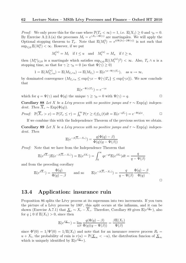
62 Lecture Notes – MS3b Levy Processes and Finance – Oxford HT 2010
Proof: We only prove this for the case where P(Tx <∞) = 1, i.e. E(X1) ≥ 0 and γ0 = 0.By Exercise A.2.3.(a) the processes Mt = eγXt−tΨ(γ) are martingales. We will apply theOptional stopping theorem to Tx. Note that E(M2
t ) = et(Ψ(2γ)−2Ψ(γ)) is not such thatsupt≥0 E(M2
t ) <∞. However, if we put
M(u)t = Mt if t ≤ u and M
(u)t = Mu if t ≥ u,
then (Mut )t≥0 is a martingale which satisfies supt≥0 E((M
(u)t )2) < ∞. Also, Tx ∧ u is a
stopping time, so that for γ ≥ γ0 = 0 (so that Ψ(γ) ≥ 0)
1 = E(M(u)Tx∧u) = E(MTx∧u) → E(MTx) = E(eγx−Ψ(γ)Tx), as u→ ∞,
by dominated convergence (MTx∧u ≤ expγx − Ψ(γ)Tx ≤ expγx). We now concludethat
E(e−Ψ(γ)Tx) = e−γx
which for q = Ψ(γ) and Φ(q) the unique γ ≥ γ0 = 0 with Ψ(γ) = q. 2
Corollary 88 Let X be a Levy process with no positive jumps and τ ∼ Exp(q) indepen-dent. Then Xτ ∼ Exp(Φ(q)).
Proof: P(Xτ > x) = P(Tx ≤ τ) =∫∞0
P(τ ≥ t)fTx(t)dt = E(e−qTx) = e−Φ(q)x. 2
If we combine this with the Independence Theorem of the previous section we obtain.
Corollary 89 Let X be a Levy process with no positive jumps and τ ∼ Exp(q) indepen-dent. Then
E(e−β(Xτ−Xτ )) =q(Φ(q) − β)
Φ(q)(q − Ψ(β))
Proof: Note that we have from the Independence Theorem that
E(eβXτ )E(e−β(Xτ−Xτ )) = E(eβXτ ) =
∫ ∞
0
qe−qtE(eβXt)dt =q
q − Ψ(β)
and from the preceding corollary
E(eβXτ ) =Φ(q)
Φ(q) − βand so E(e−β(Xτ−Xτ )) =
q
q − Ψ(β)
Φ(q) − β
Φ(q).
2
13.4 Application: insurance ruin
Proposition 86 splits the Levy process at its supremum into two increments. If you turnthe picture of a Levy process by 180, this split occurs at the infimum, and it can beshown (Exercise A.7.1) that Xτ ∼ Xτ −Xτ . Therefore, Corollary 89 gives E(eβXτ ), alsofor q ↓ 0 if E(X1) > 0, since then
E(eβX∞) = limq↓0
q(Φ(q) − β)
Φ(q)(q − Ψ(β))=βE(X1)
Ψ(β)
since Φ′(0) = 1/Ψ′(0) = 1/E(X1) and note that for an insurance reserve process Rt =u + Xt, the probability of ruin is r(u) = P(X∞ < −u), the distribution funcion of X∞which is uniquely identified by E(eβX∞).

Lecture 14
Ladder times and storage models
Reading: Kyprianou Sections 1.3.2 and 3.3
14.1 Case 1: No positive jumps
In Theorem 87 we derived the moment generating function of Tx = inft ≥ 0 : Xt > xfor any Levy process with no positive jumps. We also indicated the complication thatTx = ∞ is a possibility, in general. Let us study this is in more detail in our standardsetting
E(eγXt) = etΨ(γ), Ψ(γ) = a1γ +1
2σ2γ2 +
∫ 0
−∞(eγx − 1 − γx1|x|≤1)g(x)dx.
The important quantity is
E(X1) =∂
∂γE(eγXt)
∣∣∣∣γ=0
= Ψ′(0) = a1 −∫ 0
−1
xg(x)dx.
The formula that we derived was
E(e−qTx1Tx<∞) = e−xΦ(q)
where for q > 0, Φ(q) > 0 is unique with Ψ(Φ(q)) = q. Letting q ↓ 0, we see that
P(Tx <∞) = limq↓0
E(e−qTx1Tx<∞) = e−xΦ(0+).
Here the convexity of Ψ that we derived last time implies that Φ(0+) = 0 if and only ifE(X1) = φ′(0) ≥ 0. Therefore, P(Tx <∞) = 1 if and only if E(X1) ≥ 0.
Part of this could also be deduced by the strong (or weak) law of large numbers.Applied to increments Yk = Xkδ −X(k−1)δ it implies that
Xnδ
nδ=
1
δ
1
n
n∑
k=1
Yk →1
δE(Y1) =
1
δE(Xδ) = E(X1),
almost surely (or in probability) as n → ∞. We can slightly improve this result to aconvergence as t→ ∞ as follows
E(eγXt/t) = etφ(γ/t) → eγφ′(0) = eγE(X1) ⇒ Xt
t→ E(X1),
63

64 Lecture Notes – MS3b Levy Processes and Finance – Oxford HT 2010
in probability. We used here that Zt → a in distribution implies Zt → a in probability,which holds only because a is a constant, not a random variable. Note that indeed forall ε > 0, as t→ ∞,
P(|Zt − a| > ε) ≤ P(Zt ≤ a− ε) + 1 − P(Zt ≤ a+ ε) → 0 + 1 − 1 = 0.
From this, we easily deduce that Xt → ±∞ (in probability) if E(Xt) 6= 0, but the caseE(Xt) = 0 is not so clear from this method. In fact, it can be shown that all convergenceshold in the almost sure sense, here.
By an application of the Strong Markov property we can show the following.
Proposition 90 The process (Tx)x≥0 is a subordinator.
Proof: Let us here just prove that Tx+y − Tx is independent of Tx and has the samedistribution as Ty. The remainder is left as an exercise.
Note first that XTx = x, since there are no positive jumps. The Strong Markovproperty at Tx can therefore be stated as X = (XTx+s − x)s≥0 is independent of FTx andhas the same distribution as X. Now note that
Tx + Ty = Tx + infs ≥ 0 : Xs > y = Tx + infs ≥ 0 : XTx+s > x+ y= inft ≥ 0 : Xt > x+ y = Tx+y
so that Tx+y − Tx = Ty, and we obtain
P(Tx ≤ s, Tx+y − Tx ≤ t) = P(Tx ≤ s, Ty ≤ t) = P(Tx ≤ s)P(Ty ≤ t),
since Tx ≤ s ∈ FTx . Formally, Tx ≤ s ∩ Tx ≤ r = Tx ≤ s ∧ r ∈ Fr for all r ≥ 0since Tx is a stopping time. 2
We can understand what the jumps of (Tx)x≥0 are: in fact, X can be split into itssupremum process X t = sup0≤s≤tXs and the bits of path below the supremum. Roughly,the times
Tx, x ≥ 0 = t ≥ 0 : Xt = Xt
are the times when the supremum increases. Tx − Tx− > 0 if the supremum processremains constant at height x for an amount of time Tx − Tx−. The process (Tx)x≥0 iscalled “ladder time process”. The process (XTx)x≥0 is called ladder height process. Inthis case, XTx = x is not very illuminating. Note that (Tx, XTx)x≥0 is a bivariate Levyprocess.
Example 91 (Storage models) Consider a Levy process of bounded variation, repre-sented as At − Bt for two subordinators A and B. We interpret At as the amount ofwork arriving in [0, t] and Bt as the amount of work that can potentially exit from thesystem. Let us focus on the case where A is a compound Poisson process and Bt = tfor a continuously working processor. The quantity of interest is the amount Wt of workwaiting to be carried out and requiring storage, where W0 = w ≥ 0 is an initial amountof work stored.

Lecture 14: Ladder times and storage models 65
Note that Wt 6= w + At − Bt, in general, since w + At − Bt can become negative,whereas Wt ≥ 0. In fact, we can describe as follows: if the storage is empty, then nowork exits from the system. Can we see from At − Bt when the storage will be empty?We can express the first time it becomes empty and the first time it is refilled thereafteras
L1 = inft ≥ 0 : w + At −Bt = 0 and R1 = inft ≥ L1 : ∆At > 0.
On [L1, R1], Xt = Bt−At increases linearly at unit rate from w to w+(R1−L1), whereasW remains constant equal to zero. In fact,
Wt = w −Xt +
∫ t
L1∧t1ds = w −Xt +
∫ t
0
1Xs=Xs≥wds = (w ∨X t) −Xt, 0 ≤ t ≤ R1.
An induction now shows that the system is idle if and only if Xt = X t ≥ w, so thatWt = Xt + (w ∨Xt) for all t ≥ 0.
In this context, (X t−w)+ is the amount of time the system was idle before time t, andTx = inft ≥ 0 : Xt > x is the time by which the system has accumulated time x − win the idle state, x ≥ w, and we see that (x − w)/Tx ∼ x/Tx → 1/E(T1) = 1/Φ′(0) =φ′(0) = E(X1) = 1 − E(A1) in probability, if E(A1) ≤ 1.
Example 92 (Dams) Suppose that the storage model refers more particularly to a damthat releases a steady stream of water at a constant intensity a2. Water is added accordingto a subordinator (At)t≥0. The dam will have a maximal capacity of, say, M > 0. Givenan initial water level of w ≥ 0, the water level at time t is, as before
Wt = (w ∨X t) −Xt, where Xt = a2t−At.
The time F = inft ≥ 0 : Wt > M, the first time when the dam overflows, is a quantityof interest. We do not pursue this any further theoretically, but note that this can besimulated, since we can simulate X and hence W .
14.2 Case 2: Union of intervals as ladder time set
Proposition 93 If Xt = a2t − Ct for a compound Poisson process (Ct)t≥0 and a drifta2 ≥ 0 ∨ E(C1), then the ladder time set is a collection of intervals. More precisely,
t ≥ 0 : Xt = Xt is the range σy, y ≥ 0 of a compound Poisson subordinator with pos-itive drift coefficient.
Proof: Define L0 = 0 and then for n ≥ 0 stopping times
Rn = inft ≥ Ln : ∆Ct > 0, Ln+1 = inft ≥ Rn : Xt = X t.
The strong Markov property at these stopping times show that (Rn−Ln)n≥0 is a sequenceof Exp(λ) random variables where λ =
∫∞0g(x)dx is the intensity of positive jumps, and
(Ln − Rn−1)n≥1 is a sequence of independent identically distributed random variables.Now define Tn = R0 − L0 + . . . + Rn−1 − Ln−1 and (σy)y≥0 to be the compount Poissonprocess with unit drift, jump times Tn, n ≥ 1, and jump heights Ln − Rn−1, n ≥ 1. 2

66 Lecture Notes – MS3b Levy Processes and Finance – Oxford HT 2010
The ladder height process (Xσy)y≥0 will then also have a positive drift coefficient and
share some jump times with σ (whenever X jumps from below X t− above Xt−, but haveextra jump times when X jumps from X t− upwards, some jump times of (σy)y≥0 are notjump times of (Xσy)y≥0 – if X reaches X t− again without a jump.)
Example 94 (Storage models) In the context of the previous examples, consider moregeneral subordinators Bt with unit drift. Interpret jumps of B as unfinished work poten-tially exiting to be carried out elsewhere. We should be explicit and make a conventionthat if the current storage amount Wt is not sufficient for a jump of B, then all remainingwork exits. With this convention, the amount Wt waiting to be carried out is still
Wt = w −Xt +
∫ t
0
1Xs=Xs≥wds t ≥ 0,
but note that the latter integral cannot be expressed in terms of X t so easily, but σyis still the time by which the system has accumulated time y − w in the idle state, fory ≥ w, so It = infy ≥ 0 : σy > t is the amount of idle time before t.
14.3 Case 3: Discrete ladder time set
If Xt = a2t−Ct for a compound Poisson process (or indeed bounded variation pure jumpprocess) (Ct)t≥0 and a drift a2 < 0, then the ladder time set is discrete. We can still think
of t ≥ 0 : Xt = Xt as the range σy, y ≥ 0 of a compound Poisson subordinator withzero drift coefficient. More naturally, we would define successive ladder times G0 = 0and Gn+1 = inft > Gn : Xt = X t. By the strong Markov property, Gn+1 −Gn, n ≥ 0,is a sequence of independent and identically distributed random variables, and for anyintensity λ > 0, we can specify (σy)y≥0 to be a compound Poisson process with rate λ > 0and jump sizes Gn+1 −Gn, n ≥ 0.
Note that (σy)y≥0 is not unique since we have to choose λ. In fact, once a choice hasbeen made and q > 0, we have σy : y ≥ 0 = σqy, y ≥ 0, not just here, but also inCases 1 and 2. In Cases 1 and 2, however, we identified a natural choice (of q) in eachcase.
14.4 Case 4: non-discrete ladder time set and posi-
tive jumps
The general case is much harder. It turns out that we can still express
t ≥ 0 : Xt = X t = σy : y ≥ 0
for a subordinator (σy)y≥0, but, as in Case 3, there is no natural way to choose this process.It can be shown that the bivariate process (σy, Xσy)y≥0 is a bivariate subordinator in thisgeneral setting, called the ladder process. There are descriptions of its distribution andrelations between these processes of increasing ladder events and analogous processes ofdecreasing ladder events.

Lecture 15
Branching processes
Reading: Kyprianou Section 1.3.4
15.1 Galton-Watson processes
Let ξ = (ξk)k≥0 be (the probability mass function of) an offspring distribution. Considera population model where each individual gives birth to independent and identicallydistributed numbers of children, starting from Z0 = 1 individual, the common ances-tor. Then the (n + 1)st generation Zn+1 consists of the sum of numbers of childrenNn,1, . . . , Nn,Zn of the nth generation:
Zn+1 =Zn∑
i=1
Nn,i, where Nn,i ∼ ξ independent, i ≥ 1, n ≥ 0.
Proposition 95 Let ξ be an offspring distribution, g(s) =∑
k≥0 ξksk its generating func-
tion, then
E(sZ1) = g(s), E(sZ2) = g(g(s)), . . . ,E(sZn) = g(n)(s),
where g(0)(s) = s, g(n+1)(s) = g(n)(g(s)), n ≥ 0.
Proof: The result is clearly true for n = 0 and n = 1. Now note that
E(sXn+1) = E
(s
PZni=1Nn,i
)=
∞∑
j=0
P(Zn = j)E(s
Pji=1Nn,i
)
=
∞∑
j=0
P(Zn = j)(g(s))j = E((g(s))Zn) = g(n)(g(s)).
2
Proposition 96 (Zn)n≥0 is a Markov chain whose transition probabilities are given by
pij = P(N1 + . . .+Ni = j), where N1, . . . , Ni ∼ ξ independent.
In particular, if (Z(1)n )n≥0 and (Z
(2)n )n≥0 are two independent Markov chains with tran-
sition probabilities (pij)i,j≥0 starting from population sizes k and l, respectively, then
Z(1)n + Z
(2)n , n ≥ 0, is also a Markov chain with transition probabilities (pij)i,j≥0 starting
from k + l.
67

68 Lecture Notes – MS3b Levy Processes and Finance – Oxford HT 2010
Proof: Just note that the independence of (Nn,i)i≥1 and (Nk,i)0≤k≤n−1,i≥1 implies that
P(Zn+1 =j|Z0 = i0, . . . , Zn−1 = in−1, Zn= in) = P(Nn,1 + . . . , Nn,in =j|Z0 = i0, . . . , Zn= in)
= P(Nn,1 + . . . , Nn,in = j) = pinj ,
as required. For the second assertion note that
b(i1,i2),j := P(Z(1)n+1 + Z
(2)n+1 = j|Z(1)
n = i1, Z(2)n = i2)
= P(N(1)n,1 + . . .+N
(1)n,i1
+N(2)n,1 + . . .+N
(2)n,i2
= j) = pi1+i2,j
only depends on i1 + i2 (not i1 or i2 separately) and is of the form required to concludethat
P(Z(1)n+1 + Z
(2)n+1 = j|Z(1)
n + Z(2)n = i) =
∑ii1=0 P(Z
(1)n = i1, Z
(2)n = i− i1)b(i1,i−i1),j
P(Z(1)n + Z
(2)n = i)
= pij .
2
The second part of the proposition is called the branching property and expressesthe property that the families of individuals in the same generation evolve completelyindependently of one another.
15.2 Continuous-time Galton-Watson processes
We can also model lifetimes of individuals by independent exponentially distributed ran-dom variables with parameter λ > 0. We assume that births happen at the end of alifetime. This breaks the generations. Since continuously distributed random variablesare almost surely distinct, we will observe one death at a time, each leading to a jumpof size k − 1 with probability ξk, k ≥ 0. It is customary to only consider offspring distri-butions with ξ1 = 0, so that there is indeed a jump at every death time. Note that atany given time, if j individuals are present in the population, the next death occurs at atime
H = minL1, . . . , Lj ∼ Exp(jλ), where L1, . . . , Lj ∼ Exp(λ).
From these observations, one can construct (and simulate!) the associated populationsize process (Yt)t≥0 by induction on the jump times.
Proposition 97 (Yt)t≥0 is a Markov process. If Y (1) and Y (2) are independent Markovprocesses with these transition probabilities starting from k and l, then Y (1) +Y (2) is alsoa Markov process with the same transition probabilities starting from k + l.
Proof: Based on BS3a Applied Probability, the proof is not difficult. We skip it here.2
(Yt)t≥0 is called a continuous-time Galton-Watson process. In fact, these are the onlyMarkov processes with the branching property (i.e. satisfying the second statement ofthe proposition for all k ≥ 1, l ≥ 1).

Lecture 15: Branching processes 69
Example 98 (Simple birth-and-death processes) If individuals have lifetimes withparameter µ and give birth at rate β to single offspring repeatedly during their lifetime,then we recover the case
λ = µ+ β and ξ0 =µ
µ+ β, ξ2 =
β
µ+ β.
In fact, we have to reinterpret this model by saying each transition is a death, givingbirth to either two or no offspring. These parameters arise since, if only one individualis present, the time to the next transition is the minimum of the exponential birth timeand the exponential death time.
The fact that all jump sizes are independent and identically distributed is reminiscentof compound Poisson processes, but for high population sizes j we have high parameters tothe exponential times between two jumps – the process Y moves faster than a compoundPoisson process at rate λ. Note however that for H ∼ Exp(jλ) we have jH ∼ Exp(λ).Let us use this observation to specify a time-change to slow down Y .
Proposition 99 Let (Yt)t≥0 be a continuous-time Galton-Watson process with offspringdistribution ξ and lifetime distribution Exp(λ). Then for the piecewise linear functions
Jt =
∫ t
0
Yudu, t ≥ 0, ϕs = inft ≥ 0 : Jt > s, 0 ≤ s < J∞,
the process
Xs = Yϕs, 0 ≤ s < J∞,
is a compound Poisson process with jump distribution (ξk+1)k≥−1 and rate λ, run untilthe first hitting time of 0.
Proof: Given Y0 = i, the first jump time T1 = inft ≥ 0 : Yt 6= i ∼ Exp(iλ), so
JT1 = iT1 and ϕs = s/i, 0 ≤ s ≤ iT1,
so we identify the first jump of Xs = Ys/i, 0 ≤ s ≤ iT1 at time iT1 ∼ Exp(λ).
Now the strong Markov property (or the lack of memory property of all other life-times) implies that given k offspring are produced at time T1, the process (YT1+t)t≥0 isa continuous-time Galton-Watson process starting from j = i + k − 1, independent of(Yr)0≤r≤T1 . We repeat the above argument to see that T2 − T1 ∼ Exp(jλ), and for j ≥ 1,
JT2 = iT1 + j(T2 − T1) and ϕiT1+s = T1/i+ s/j, 0 ≤ s ≤ j(T2 − T1),
and the second jump of XiT1+s = YT1+s/j, 0 ≤ s ≤ j(T2 − T1), happens at time iT1 +j(T2 − T1), where j(T2 − T1) ∼ Exp(λ) is independent of iT1. An induction as long asYTn > 0 shows that X is a compound Poisson process run until the first hitting time of0. 2

70 Lecture Notes – MS3b Levy Processes and Finance – Oxford HT 2010
Corollary 100 Let (Xs)s≥0 be a compound Poisson process starting from l ≥ 1 with jumpdistribution (ξk+1)k≥−1 and jump rate λ > 0. Then for the piecewise linear functions
ϕs =
∫ s
0
1
Xvdv, 0 ≤ s < T0, and Jt = infs ≥ 0 : ϕs > t, t ≥ 0,
the process
Yt = XJt , t ≥ 0,
is a continuous-time Galton-Watson process with offspring distribution ξ and lifetimedistribution Exp(λ).
15.3 Continuous-state branching processes
Population-size processes with state space N are natural, but for large populations, it isoften convenient to use continuous approximations and use a state space [0,∞). In viewof Corollary 100 it is convenient to define as follows.
Definition 101 (Continuous-state branching process) Let (Xs)s≥0 be a Levy pro-cess with no negative jumps starting from x > 0, with E(exp−γXs) = expsφ(γ).Then for the functions
ϕs =
∫ s
0
1
Xv
dv, 0 ≤ s < T0, and Jt = infs ≥ 0 : ϕs > t, t ≥ 0,
the process
Yt = XJt , t ≥ 0,
is called a continuous-state branching process with branching mechanism φ.
We interpret upward jumps as birth events and continuous downward movement as(infinitesimal) deaths. The behaviour is accelerated at high population sizes, so fluc-tuations will be larger. The behaviour is slowed down at small population sizes, sofluctuations will be smaller.
Example 102 (Pure death process) For Xs = x− cs we obtain
ϕs =
∫ s
0
1
x− cvdv = −1
clog(1 − cs/x), and Jt =
x
c(1 − e−ct),
and so Yt = xe−ct.
Example 103 (Feller diffusion) For φ(γ) = γ2 we obtain Feller’s diffusion. There arelots of parallels with Brownian motion. There is a Donsker-type result which says thatrescaled Galton-Watson processes converge to Feller’s diffusion. It is the most popularmodel in applications. A lot of quantities can be calculated explicitly.
Proposition 104 Y is a Markov process. Let Y (1) and Y (2) be two independent continuous-state branching processes with branching mechanism φ starting from x > 0 and y > 0.Then Y (1) + Y (2) is a continuous-state branching process with branching mechanism φstarting from x+ y.

Lecture 16
The two-sided exit problem
Reading: Kyprianou Chapter 8, Bertoin Aarhus Notes, Durrett Sections 7.5-7.6
16.1 The two-sided exit problem for Levy processes
with no negative jumps
Let X be a Levy process with no negative jumps. As we have studied processes with nopositive jumps (such as −X) before, it will be convenient to use compatible notation andwrite
E(e−γXt) = etφ(γ), φ(γ) = a−Xγ +1
2σ2γ2 +
∫ 0
−∞(eγx − 1 − γx1|x|≤1)g−X(x)dx
= −aXγ +1
2σ2γ2 −
∫ ∞
0
(1 − e−γx − γx1|x|≤1)gX(x)dx,
where a−X = −aX and gX(x) = g−X(−x), x > 0. Then we deduce from Section 11.4that, if E(X1) < 0,
E(e−βX∞) = −βE(X1)
φ(β), β ≥ 0. (1)
The two-sided exit problem is concerned with exit from an interval [−a, b], notably thetime
T = T[−a,b]c = inft ≥ 0 : Xt ∈ [−a, b]c
and the probability to exit at the bottom P(XT = −a). Note that an exit from [−a, b]at the bottom happens necessarily at −a, since there are no negative jumps, whereas anexit at the top may be due to a positive jump across the threshold b leading to XT > b.
Proposition 105 For any Levy process X with no negative jumps, all a > 0, b > 0 andT = T[−a,b]c, we have
P(XT = −a) =W (b)
W (a+ b), where W is such that
∫ ∞
0
e−βxW (x)dx =1
φ(β).
71

72 Lecture Notes – MS3b Levy Processes and Finance – Oxford HT 2010
Proof: We only prove the case E(X1) < 0. By (1), we can identify (the right-continuousfunction) W , since
−βE(X1)
φ(β)= E(e−βX∞) =
∫ ∞
0
e−βxfX∞(x)dx
=
∫ ∞
0
βe−βxP(X∞) ≤ x)dx,
by partial integration, and so by the uniqueness of moment generating functions, we haveW (x) = cP(X∞ ≤ x), where c = −E(X1) > 0.
Now define τa = inft ≥ 0 : Xt < −a and apply the strong Markov property at τa to
get a post-τa process X = (Xτa+s + a)s≥0 independent of (Xr)r≤τa , in particular of Xτa ,so that
cW (b) = P(X∞ ≤ b) = P(Xτa ≤ b, X∞ ≤ a+ b)
= P(Xτa ≤ b)P(X∞ ≤ a + b) = P(Xτa ≤ b)cW (a+ b),
and the result follows. 2
Example 106 (Stable processes) Let X be a stable process of index α ∈ (1, 2] withno negative jumps, then we have
∫ ∞
0
e−λxW (x)dx = λ−α ⇒ Γ(α)W (x) = xα−1.
We deduce that
P(XT = −a) =
(b
a+ b
)α−1
.
16.2 The two-sided exit problem for Brownian mo-
tion
In the Brownian case, we can push the analysis further without too much effort.
Proposition 107 For Brownian motion B, all a > 0, b > 0 and T = T[−a,b]c, we have
E(e−qT |BT = −a) =Vq(b)
Vq(a + b)and E(e−qT |BT = b) =
Vq(a)
Vq(a+ b),
where
Vq(x) =sinh(
√2qx)
x.

Lecture 16: The two-sided exit problem 73
Proof: We condition on BT and use the strong Markov property of B at T to obtain
e−a√
2q = E(e−qT−a)
= P(BT = −a)E(e−qT−a |BT = −a) + P(BT = b)E(e−qT−a|BT = b)
=b
a + bE(e−qT |BT = −a) +
a
a + bE(e−q(T+ eT−a−b)|BT = b)
=b
a + bE(e−qT |BT = −a) +
a
a + bE(e−qT |BT = b)e−(a+b)
√2q
and, by symmetry,
e−b√
2q =a
a+ bE(e−qT |BT = b) +
b
a+ bE(e−qT |BT = −a)e−(a+b)
√2q.
These can be written as
b+ a
ab= a−1E(e−qT |BT = −a)ea
√2q + b−1E(e−qT |BT = b)e−b
√2q
b+ a
ab= a−1E(e−qT |BT = −a)e−a
√2q + b−1E(e−qT |BT = b)eb
√2q
and suitable linear combinations give, as required,
2 sinh(a√
2q)b+ a
ab= 2 sinh((a + b)
√2q)b−1E(e−qT |BT = b)
2 sinh(b√
2q)b+ a
ab= 2 sinh((a + b)
√2q)a−1E(e−qT |BT = −a).
2
Corollary 108 For Brownian motion B, all a > 0 and T = T[−a,a]c, we have
E(e−qT ) =1
cosh(a√
2q)
Proof: Just calculate from the previous proposition
E(e−qT ) =Vq(a)
Vq(2a)= 2
e√
2qa − e−√
2qa
(e√
2qa)2 − (e−√
2qa)2=
1
cosh(a√
2q).
2
16.3 Appendix: Donsker’s Theorem revisited
We can now embed simple symmetric random walk (SSRW) into Brownian motion B byputting
T0 = 0, Tk+1 = inft ≥ Tk : |Bt −BTk| = 1, Sk = BTk
, k ≥ 0,
and for step sizes 1/√n modify T
(n)k+1 = inft ≥ T
(n)k : |Bt − B
T(n)k
| = 1/√n.

74 Lecture Notes – MS3b Levy Processes and Finance – Oxford HT 2010
Theorem 109 (Donsker for SSRW) For a simple symmetric random walk (Sn)n≥0
and Brownian motion B, we have
S[nt]√n
→ Bt, locally uniformly in t ≥ 0, in distribution as n→ ∞.
Proof: We use a coupling argument. We are not going to work directly with the originalrandom walk (Sn)n≥0, but start from Brownian motion (Bt)t≥0 and define a family ofembedded random walks
S(n)k := B
T(n)k
, k ≥ 0, n ≥ 1, ⇒(S
(n)[nt]
)
t≥0∼(S[nt]√n
)
t≥0
.
To show convergence in distribution for the processes on the right-hand side, it suffices toestablish convergence in distribution for the processes on the left-hand side, as n→ ∞.
To show locally uniform convergence we take an arbitrary T ≥ 0 and show uniformconvergence on [0, T ]. Since (Bt)0≤t≤T is uniformly continuous (being continuous on acompact interval), we get in probability
sup0≤t≤T
∣∣∣S(n)[nt] −Bt
∣∣∣ = sup0≤t≤T
∣∣∣∣BT(n)[nt]
− Bt
∣∣∣∣ ≤ sup0≤s≤t≤T :|s−t|≤sup0≤r≤T |T (n)
[nr]−r|
|Bs − Bt| → 0
as n→ ∞, if we can show (as we do in the lemma below) that sup0≤t≤T |T (n)[nt] − t| → 0.
This establishes convergence in probability, which “implies” convergence in distribu-tion for the embedded random walks and for the original scaled random walk. 2
Lemma 110 In the setting of the proof of the theorem, sup0≤t≤T |T(n)[nt] − t| → 0 in prob-
ability.
Proof: First for fixed t, we have
E(e−qT (n)
[nt]) =(
E(e−qT(n)1 ))[nt]
=1
(cosh(√
2q/n))[nt]→ e−qt,
since cosh(√
2q/n) ∼ 1 + q/n+ O(1/n). Therefore, in probability T(n)[nt] → t. For unifor-
mity, let ε > 0. Let δ > 0. We find n0 ≥ 0 such that for all n ≥ n0 and all tk = kε/2,1 ≤ k ≤ 2T/ε we have
P(|T (n)[ntk] − tk| > ε/2) < δε/2T,
then
P
(sup
0≤t≤T|T (n)
[nt] − t| > ε
)≤ P
(sup
1≤k≤2T/ε
|T (n)[ntk] − tk| >
ε
2
)≤
2T/ε∑
k=1
P
(|T (n)
[ntk] − tk| >ε
2
)< δ.
2
We can now describe the recipe for the full proof of Donsker’s Theorem. In fact, wecan embed every standardized random walk ((Sk − kE(S1))/
√nVarS1)k≥0 in Brownian
motion X, by first exits from independent random intervals [−A(n)k , B
(n)k ] so that X
T(n)k
∼(Sk − kE(S1))/
√nVar(S1), and the embedding time change (T
(n)[nt])t≥0 can still be shown
to converge uniformly to the identity.