more efficient on-the-fly ltl verification with tarjan's algorithm

Theoretical Computer Science 345 (2005) 60–82www.elsevier.com/locate/tcs

More efficient on-the-fly LTL verification withTarjan’s algorithm

Jaco Geldenhuys∗, Antti ValmariTampere University of Technology, Institute of Software Systems, PO Box 553, FI-33101 Tampere, Finland

Abstract

State-of-the-art algorithms for on-the-fly automata-theoretic LTL model checking make use ofnested depth-first search to look for accepting cycles in the product of the system and the Büchiautomaton. Here, we present two new single depth-first search algorithms that accomplish the sametask. The first is based on Tarjan’s algorithm for detecting strongly connected components, while thesecond is a combination of the first and Couvreur’s algorithm for finding acceptance cycles in theproduct of a system and a generalized Büchi automaton. Both new algorithms report an acceptingcycle immediately after all transitions in the cycle have been investigated. We show their correctness,describe efficient implementations and discuss how they interact with some other model checkingtechniques, such as bitstate hashing. The algorithms are compared to the nested search algorithms inexperiments on both random and actual state spaces, using random and real formulas. Our measure-ments indicate that our algorithms investigate at most as many states as the old ones. In the case of aviolation of the correctness property, the algorithms often explore significantly fewer states.© 2005 Elsevier B.V. All rights reserved.

Keywords:Model checking; Verification

1. Introduction

Explicit-state on-the-fly automata-theoretic LTL model checking relies on two algo-rithms: the first for constructing an automaton that represents the negation of the correct-ness property, and the second for checking that the language recognized by the product of

∗ Corresponding author.E-mail addresses:[email protected](J. Geldenhuys),[email protected](A. Valmari).

0304-3975/$ - see front matter © 2005 Elsevier B.V. All rights reserved.doi:10.1016/j.tcs.2005.07.004

http://www.elsevier.com/locate/tcs

mailto:[email protected]

mailto:[email protected]

J. Geldenhuys, A. Valmari / Theoretical Computer Science 345 (2005) 60–82 61

the system and the automaton is empty. This amounts to verifying that the system has noexecutions that violate the correctness property. An algorithm for converting LTL formulasto Büchi automata was first described in[33], and many subsequent improvements havebeen proposed [6,10,12,14,26,28].Checking the emptiness of the product automaton requires checking that none of its

cycles contains any accepting states. One approach to this problem is to detect thestronglyconnected components(SCC) of the product. An SCC is a maximal setC of states suchthat for all s1, s2 ∈ C there is a path froms1 to s2. An SCC is said to benontrivial ifit contains at least one such nonempty path, and, conversely, an SCC istrivial when itconsists of a single state without a self-loop. The two standard methods of detecting SCCsare Tarjan’s algorithm [1,29], and the double search algorithm attributed to Kosaraju andfirst published in [27]. Both approaches often appear in textbooks. There is also a lesswell-known algorithm by Dijkstra [7].Unfortunately, both of the well-known algorithms have aspects that discourage their

use for on-the-fly model checking. Tarjan’s algorithm makes copious use of stack space,while Kosaraju’s algorithm needs to explore transitions backwards. Instead, state-of-the-artalgorithms perform nested depth-first searches [3,21].In this paper, we introduce two new algorithms for detecting accepting cycles. The first

was originally published in [13] in a slightly less efficient version. It is based on Tarjan’salgorithm, but, because it relies on a single depth-first search and it tends to detect violationsearly, its time and memory requirements are often smaller than those of its competitors. Infact, we show that, if an accepting cycle exists, our algorithm will report it as soon as alltransitions of the cycle have been investigated. (This is not true of the nested search algo-rithms.) In other words, provided that transitions of the product automaton are investigatedin the same order (which may be any depth-first order), no algorithm can report a violationsooner than ours.The second new algorithm is a combination of the first algorithm and Couvreur’s similar

algorithm for generalizedBüchi automata [5]. LikeCouvreur’s algorithm, it is basedon ideasin [7]. Its memory consumption is less than that of either the first algorithm or Couvreur’s.The rest of this article is organized as follows: In Section 2, we describe the standard

nested depth-first search algorithm, and discuss its strengths and weaknesses. Section 3contains the first of our new algorithms and a proof of its correctness. In Section 4, weconsider Couvreur’s algorithm and in Section 5 present the second of our new algorithms.Some implementation issues, plus the generation of counterexamples, are discussed inSection 6. Experimental results are given in Section 7, and we explore the use of heuristicsfor speeding up the detection of violations in Section 8. Finally, Section 9 presents ourconclusions.

2. The CVWY algorithm

Courcoubetis et al. [3,4] presented the nested depth-first search algorithm for detectingaccepting cycles shown in Fig. 1. In the rest of this paper we shall refer to this algorithmby the moniker “CVWY”. The algorithm is based on a standard depth-first search. Whena state has been fully explored and if the state is accepting, a second search is initiated todetermine whether it is reachable from itself and in this way forms an accepting cycle.

62 J. Geldenhuys, A. Valmari / Theoretical Computer Science 345 (2005) 60–82

DFS(s)1 MARK(〈s,0〉)2 for each successort of s do3 if ¬MARKED(〈t,0〉) then4 DFS(t)5 if ACCEPTING(s) then6 seed:= s ; NDFS(s)

NDFS(s)7 MARK(〈s,1〉)8 for each successort of s do9 if ¬MARKED(〈t,1〉) then10 NDFS(t)11 else if t = seedthen12 report violation

Fig. 1. The nested depth-first search algorithm of[3].

The algorithm is clearly suited to on-the-fly verification. For each state, only two bitsof information is required to record whether it has been found during the first and duringthe second search. Even when Holzmann’s bitstate hashing technique[19,20] is used, hashcollisions will not cause the algorithm to incorrectly report a violation. CVWY also makessequential use of the stack, which means that it can be swapped to disk, leaving the mainmemory available for recording the visited states.A disadvantage of CVWY is that it does not find violations before starting to backtrack.

Because depth-first search paths can grow rather long, many states may be on the stackat the time the first violation is detected, thus increasing time and memory consumption,and producing long counterexamples. It is not easy to change this behaviour, because itis important for the correctness of CVWY that, when checking an accepting state for acycle, accepting states that are “deeper” in the depth-first search tree have already beeninvestigated.Tarjan’s algorithm also detects completed SCCs starting with the “deepest”, but it per-

forms only a single depth-first search and can already detect states that belong to the sameSCC “on its way down”, which is why it needs to “remember” the states by placing themon a second stack. Such early detection of partial SCCs, and by implication, of acceptingcycles, is desirable, because intuitively it seems that, not only could it reduce memory andtime consumption, but could also produce smaller counterexamples.

3. Cycle detection with Tarjan’s algorithm

3.1. Motivation

Tarjan’s algorithm is often mentioned but dismissed as too memory consuming to beconsidered useful, as, for example, in [4,16]. In the presentation of Tarjan’s algorithm in[1, Chapter 5.5] states are placed on an explicit stack in addition to being placed on theimplicit proceduralstack—that is, the runtimestack that implements procedure calls.More-over, a state remains on the explicit stack until its entire SCC has been explored. Only when


Fig. 2. The component and product automata of the alternating bit protocol.

the depth-first search is about to leave a state (in other words, the state has been fully ex-plored) and the algorithm detects that it is the root of an SCC, the state and all its SCCmembers are removed from the explicit stack. In consequence, the explicit stack may con-tain several partial SCCs—many more states than the implicit depth-first stack. In addition,each state has two associated attributes: its depth-first number, and itslowlink value; natu-rally these require extra memory. There is also a marked flag, but in state space applicationsthe same information is obtained by checking whether the state has been constructed.However, we believe it is wrong to dismiss Tarjan’s algorithm too quickly. Firstly, it is

true that the state space of the system under investigation often forms a single, large SCC.But the product automaton in which the accepting SCC must be detected is often brokeninto many smaller SCCs by the interaction of the system with the Büchi automaton.This factoring of the product automaton is illustrated in Fig.2 (excluding the dashed

arrows).SenderandReceiverare two processes that communicate using the alternating bitprotocol [2], and the Büchi automaton for the negation of the LTL property�♦p appearsat the top right. SR denotes “send request”, RI denotes “receive indication”, and Dxand Axdenote data transmission and acknowledgment, respectively, with alternation bitx. The statelabels of the product automaton reflect the local states of the three participating automata,and for clarity, only some of the product transitions are labeled. While the processes (andtheir product which is not shown) have one SCC each, and the Büchi automaton has twoSCCs, the final product automaton has eight SCCs, one consisting of the nonacceptingstates, and seven trivial SCCs each consisting of one accepting state. (Even when a systemand a Büchi automaton each consist of a single SCC it is still possible that their productwill have more than one component, as the Büchi transitions are enabled and disabled bythe values of the atomic propositions.)


Secondly, and most importantly, for the automata-theoretic approach to work it is un-necessary to compute the entire SCC of a violating accepting cycle—it suffices todetectanontrivial SCC that contains an accepting state. To illustrate this, assume that the dashedarrows are added to Fig.2 (modelling the possibility of D0 being sent but lost). The CVWYalgorithm must investigate a path down to state 342 before it starts backtracking and de-tecting errors, whereas Tarjan’s algorithm needs to explore only states 111 and 212 andtwo transitions, if the depth-first search happens to investigate the transitions in a suitableorder.While these arguments do not constitute a claim that Tarjan’s algorithm is necessarily

viable, they do open the door to investigating its potential.

3.2. The new algorithm

We now present the first new algorithm, which we shall callTCHECK, in considerabledetail. Our presentation in Fig. 3 differs from the original presentation of Tarjan’s algo-rithm [1,29] and from the usual presentation of nested search algorithms in that it is iterativeand not recursive. We believe that it is important to address the memory requirements thatare often hidden by recursion. The data structures of the new algorithm are shown in Fig. 4.Apart from the iterativeness and the level of detail presented, however, there are other, moresignificant, conceptual differences—so many that we chose to prove the correctness of ouralgorithm from scratch in Section 3.3:(1) The original algorithm permanently associates three attributes with each state: the

marked(s) attribute is a flag that indicates whether states has been encountered bythe depth-first search; all states are numbered consecutively in the order that they areencountered anddfnumber(s) stores that number ofs, known as the depth-first num-ber; andlowlink(s) stores the lowlink value ofs. Our algorithm dispenses withmarkedanddfnumberby representing the information implicitly, and only keeps track of thelowlink of s as long as it is necessary.

(2) As in Tarjan’s algorithm partial SCCs are stored on an explicit stack, implemented bythecstackarray. The index of its topmost element is stored inctop. We refer to this asthe component stack. Each entry ofcstackstores thestateitself and itslowlink value.To search the stack efficiently, each entry also has anextfield which stores the indexof the next entry in a hash list, and the hash lists are rooted in thechasharray.

(3) A state’s position incstackplays the same role in our algorithm as its depth-first numberdoes in Tarjan’s algorithm. The positions are not always the same as Tarjan’s depth-firstnumbers, but, since states are placed oncstackthe first time they are encountered, theorder of the positions and the order of the depth-first numbers are the same. In bothTarjan’s and our algorithm this attribute of states plays no role after they have beenremoved from the explicit stack.

(4) The implicit procedural stack used for recursion is replaced bydstack(whose topmostelement index isdtop); we refer to this as the depth-first stack. Unlikecstack, this is aproper stack in the sense that only the top element is accessed. Since the depth-first stackis a subset of the component stack, its entries need not duplicate the state information,but instead store the index of the correspondingcstackentry in fieldpos. Thelasttr fieldof dstackkeeps track of the last transition executed in each of the states on the current


DStack= recordlasttr: Transitionpos: integer

endrecord

CStack= recordlowlink: integerstate: Statenext: integer

endrecord

1 dtop: integer := −1; dstack: stack of DStack2 ctop: integer := −1; cstack: array [0 . . .] of CStack3 atop: integer := −1; astack: stack of integer4 chash: array [0 . . . K−1] of integer := [−1, . . . ,−1]5 store: set ofState:= ∅6 violation: boolean:= false

TCHECK(s0)7 PUSH(s0)8 while dtop� 0 and¬violationdo9 s′ := NEXTTRANS(dtop)10 if s′ = “no more” then POP ; goto line811 p := chash[HASH(s′)]12 while p = −1 and cstack[p].state = s′ do p := cstack[p].next13 if p = −1 then UPDATE(p) ; goto line814 if ¬store.CONTAINS(s′) then PUSH(s′)15 if violation then report violation

UPDATE(t)16 f := dstack[dtop].pos17 if cstack[t].lowlink � cstack[f ].lowlink then18 violation := (atop � 0 and t � astack[atop])19 cstack[f ].lowlink := cstack[t].lowlink

PUSH(s)20 ctop := ctop+ 121 cstack[ctop].lowlink := ctop22 cstack[ctop].state:= s

23 h := HASH(s)

24 cstack[ctop].next := chash[h]25 chash[h] := ctop26 dtop := dtop+ 127 dstack[dtop].lasttr := “none yet”28 dstack[dtop].pos:= ctop29 if ACCEPTING(s) then30 atop := atop+ 131 astack[atop] := ctop

POP

32 p := dstack[dtop].pos33 dtop := dtop− 134 if cstack[p].lowlink = p then35 while ctop� p do36 h := HASH(cstack[ctop].state)37 chash[h] := cstack[ctop].next38 store.INSERT(cstack[ctop].state)39 ctop := ctop− 140 if atop� 0 and p = astack[atop] then41 atop := atop− 142 if dtop� 0 then UPDATE(p)

Fig. 3. A new algorithm for detecting accepting cycles.

depth-first search path; it is the analogue of the implicit, local control variable of thefor loop in line2 of Fig. 1. The algorithm uses functionNEXTTRANS to generate thenext successor of the state at the top ofdstack. This function simultaneously updatesthelasttr field. The generation of the next transition may be complicated—particularlyif advanced verification methods such as symmetries or partial order/stubborn sets areused—but the details are beyond the scope of this article.


Fig. 4. The data structures of the first new algorithm.

(5) Whereas the original algorithm merely marks states as “old”, our algorithm overtly in-serts the states incstack, and later on moves them to thestore data structure(lines22, 38). The reason for this difference is that Tarjan assumes an explicit graphwhereas in state space methods the nodes of the graph (i.e., the states) are constructedon-the-fly.

(6) Line 13 of our algorithm omits a test made by Tarjan’s algorithm to avoid the updatefor descendants ofs that have already been investigated (“forward edges” in depth-firstsearch terminology). This change is harmless, since thelowlink values of such stateshave already been propagated back tos, and the omission does not affect the correctnessof the algorithm.

(7) When a transition from statef to statet is encountered, Tarjan’s algorithm sometimesupdates the lowlink off with the depth-first number oft , and sometimes with thelowlink value of t . However, in our algorithm it is always the lowlink oft that is usedfor the update (lines17–19). A similar change has been described in [24].

(8) The most important new element in our algorithm is theastackstack. It stores theindices of all the accepting states on the current depth-first search path in their depth-first order, and, likedstack, it too is a proper stack. The topmost element ofastackactsas a threshold for detecting a violation: when a transition from the current state to astate at or below this threshold is investigated, an accepting cycle has been found andthe algorithm can report a violation.

3.3. Correctness

We start by establishing some properties of the algorithm that are always true whenexecution reaches line8. Each of the properties can be shown to be correct directly fromthe code and the preceding properties, without appealing to the overall operation of thealgorithm.

Lemma 1. Whenever execution of theTCHECKalgorithm reaches line8,all of the followingproperties hold:(a) dtop� − 1∧ atop� − 1.


(b) ctop� − 1∧ ∀i ; 0� i � dtop : dstack[i].pos� 0.(c) dstack[0].pos < dstack[1].pos < · · · < dstack[dtop].pos� ctop.(d) The contents of astack is exactly the pos-fields of those dstack entries that correspond

to accepting states.(e) ∀ h ; 0� h < K : −1� chash[h] � ctop

∧ ∀i ; 0� i � ctop : −1� cstack[i].next< i∧ each0� i � ctop appears exactly once in the chash lists.

(f) A state may be in and move between data structures only like this:

nowhere→ chash lists→ store.

(g) The algorithm visits the states in depth-first order. In particular, if 0� i < dtop, thenthere is a transition from cstack[dstack[i].pos].state to cstack[dstack[i + 1].pos].state.

(h) While a state is in cstack in positioni, its lowlink is between0 and i, and it does notgrow.

(i) If violation = false, then for every0� i � ctop it holds that either cstack[i].lowlink =i, or none of the states in positions cstack[i].lowlink . . . i is accepting.

Proof.(a) From lines1, 3; 26, 30; 8, 33, 40, 41.(b) From lines2; 20, 28; 32, 35, 39.(c) PUSHmakes theposfield of the newdtopgreater than the oldctopand thus greaterthan thepos field of the old dtop. POP guarantees that ifctop decreases, then atthe end ofPOP (unlessdtop = −1), dstack[dtop].pos < p and ctop = p − 1, sodstack[dtop].pos� ctop.

(d) Theastackclaim can be seen correct by comparing the processing ofastackto that ofdstack.

(e) Whenever a state is added to one ofcstackor chash, it is added to both, and the sameholds for removals. The addition guarantees thatcstack[i].next< i, which guaranteesthat the removal operation removes only the correct entry fromchash.

(f) The only places where states are added to or removed from data structures are lines7,14, and 36–39. The first two add the state tochashafter it has been verified thatit was nowhere else. The last implements the other possibility: a move fromchashto store.

(g) PUSHcorresponds to going forward andPOPto backtracking. The order in which outputtransitions of a state are investigated is determined by theNEXTTRANS function.

(h) From lines17, 19; 21.(i) As long as a state is incstackin positioni, the acceptance status of the states in po-sitions � i does not change. Consider the first moment when at the end of line19,there is ana such thatcstack[f ].lowlink � a � f andcstack[a].stateis accepting. Soa � cstack[t].lowlink.Because this is thefirst time, it cannotbe thatcstack[t].lowlink �a < t , soa � t . By line 16 and Lemma 1(c, d),atop� 0 andastack[atop] � a � t . Soviolationbecomestrue. �

To reason about the overall operation of the algorithm, we make use of colours. Thecolours are not in any way essential to the operation of the algorithm; they are simply


mental tools that help us to understand that the algorithm is correct. A state can have oneof the following colours:• White: the state has not been found yet;• Grey: the state is present on the component stack (that is,∃i ; 0� i � ctop : cstack[i].

state= state) and there is a corresponding entry on the depth-first stack that points to thecomponent stack entry;

• Brown: the state is present on the component stack, but not on the depth-first stack; and• Black: the state is instore.

Lemma 2. The colour of a state may only change from white to grey, from grey to brownor black, and from brown to black.

Proof. Becausebeing inchashis equivalent (byLemma1(e)) tobeing incstack, Lemma1(f)implies that only changes from white to grey or brown, grey or brown to black and betweengrey and brown are possible. A change from white to brown is impossible, because, when astate is added tocstack, it is simultaneously added todstack. A change from brown to greyis ruled out because when a state is added todstack, it was verified at lines 11–13 that itwas not incstack. �

If s ands′ are two states in the state space, then by “s can reachs′” we mean that thereis a path froms to s′ in the state space.

Lemma 3. Let s be the state on cstack at positionk.(a) s can reach the state at position cstack[k].lowlink.(b) If s is brown, it can reach a state strictly below itself on cstack.(c) If s is grey, it can reach all states above it on cstack.(d) s can reach all states above it on cstack.

Proof.

(a) Via the path by which theUPDATEoperations propagated the lowlink value back tok.(b) Whens is painted brown,cstack[k].lowlink < k, by Lemma1(h) and line 34. Thus,

the claim follows from (a).(c) This is true initiallywhencstackis empty.Whenawhite states is placedon top ofcstackand becomes grey, the lemma holds fors because there are no states above it. Othergrey states can reach the previousdstack[dtop].posand thus alsos via the transitionjust explored.

(d) A state oncstackis either grey or brown. If it is grey, then the result holds by (c). If itis brown, then repeated application of (b) eventually leads to a grey state that is belows and reachable froms, from which (c) gives the claim.�

This lemma implies that the topmost grey state incstackand all states above it belong tothe same SCC.

Theorem 4. If the algorithm announces a violation, then there is an accepting cycle.


Proof. Consider line18. By Lemma 3(d)t can reachastack[atop] which can reachf byLemmas 1(d) and 3(d). The transition that caused the announcement is fromf to t, closingthe cycle. �

Lemma 5. If a state is black, then all states reachable from it are black.

Proof. The lemma holds initially when all states are white. Since black states do not everchange colour, it suffices to consider whether the lemma is violated when more states arebeing painted black (procedurePOP, lines35–39). At this point,cstack[p].lowlink = p

andp was just painted brown, andp + 1 . . . ctopare brown (Lemma 1(c)). Only the tran-sitionsq → r, whereq is any ofp . . . ctop andr is neither black nor any ofp . . . ctopare dangerous for the lemma, so consider any one of them. Becauseq is beingPOP’dor has beenPOP’d (is brown), r cannot be white (line 10). The only possibility that re-mains is thatr is one of 0. . . p − 1. But then the lowlink ofq was made at mostp − 1when theq → r transition was investigated, from which line 42 has propagated it (or asmaller value) back top. This contradicts line 34 and therefore such a transition cannotexist. �

This implies thatPOPremoves states fromcstackone SCC at a time.We shall now prove a theorem saying that if there are accepting cycles, the algorithm

will find one and, what is more, do so “as soon as possible”. To make “as soon as possi-ble” precise we define that “investigating a transition froms to s′” means the executionof line 13 (and possibly line 14) whilecstack[dstack[dtop].pos].state = s. We say thatthe algorithm “closes an accepting cycle” if there are statess1, s2, . . . , sn such that at leastone of them is accepting (call itsA), s1 → s2 → · · · → sn are transitions that the al-gorithm has investigated, andsn → s1 is a transition that the algorithm is investigating.(If the transitionsn → s1 occurs more than once in an accepting cycle, then the subcy-cle starting at the last instance ofs1 at or beforesA and ending with the first instanceof sn at or aftersA satisfies the description.) These notions extend to any graph searchalgorithm.

Lemma 6. For each SCC, whenTCHECK closes an accepting cycle within the SCC for thefirst time, p = −1 and at least one of the states in positions� p of cstack is accepting.

Proof. For 1� i � n, the statesi is neither black, because it can reach the grey statesn (Lemma5), nor white, because either it issn or the transitionsi → si+1 has beeninvestigated.p is the position ofs1 in cstack. Thus,p = −1. Leta be the position ofsA incstack. If a < p, then there has been a time whens1 was the top state ofdstackandsA wasbelow it. By Lemma 3(d), a path fromsA to s1 had been investigated already by then. Thispath together withs1 → · · · → sA is an accepting cycle, which contradicts the assumption“the first time”. �

Theorem 7. If there is an accepting cycle, then algorithmTCHECK reports a violation.Furthermore, it reports a violation immediately after the underlying depth-first search hasinvestigated all transitions of any accepting cycle.


Proof. Because the algorithm is a depth-first search, it will eventually close an accept-ing cycle, if there is any. Lemma6 implies that when the algorithm closes anaccepting cycle for the first time, line 13 will callUPDATE. Leta andp be as in the proof ofLemma 6. We havet = p, f = dstack[dtop].pos, anda � t . If the condition on line 17 didnot hold, thencstack[f ].lowlink < cstack[t].lowlink � t � a � dstack[dtop].pos = f ,contradicting Lemma 1(i). So the execution will continue to line 18, which will setviolationto true. �

4. Couvreur’s algorithm

After the initial publicationof our results [13],we learnedof similarworkbyCouvreur [5].Like our TCHECK, Couvreur’s algorithm is based on a single depth-first search and detectsaccepting cycles. The algorithm as shown in Fig. 5 was taken from [5]; apart from minorchanges in notation, the only difference is that we have combined Couvreur’sroot andarcstacks into one stack,rootarc.

COUVREUR

1 n := 12 hash.SET(s0,1)3 rootarc.PUSH(1,∅,∅)4 EXPLORE(s0,1)

EXPLORE(s, v)5 for each successor〈t, A〉 of s do6 w := hash.GET(t)7 if w = “none” then8 n := n+ 19 hash.SET(t, n)10 rootarc.PUSH(n,∅, A)11 EXPLORE(t, n)12 else ifw = 0 then13 (i, B, C) := rootarc.POP ; B := B ∪ A14 while i > w do15 B := B ∪ C16 (i, A,C) := rootarc.POP ; B := B ∪ A17 rootarc.PUSH(i, B, C)18 if B = ALL_ACC_SETS then report violation19 (i,__,__) := rootarc.TOP20 if v = i then21 n := v − 122 rootarc.POP23 REMOVE(s)

REMOVE(s)24 if hash.GET(s) = 0 then25 hash.SET(s,0)26 for each successor〈t, A〉 of s do REMOVE(t)

Fig. 5. Couvreur’s algorithm [5].


Couvreur’s algorithm differs fromTCHECKin two significant aspects. Firstly, whereas ouralgorithm is intended for use with a standard Büchi automaton (BA), Couvreur’s algorithmis geared towards ageneralizedBüchi automaton (GBA). The crucial difference betweena BA and a GBA is that while the former has only a single set of accepting states, thelatter may have many acceptance sets, each a subset of the states of the automaton, andnot necessarily mutually disjoint. Each state of a GBA may therefore belong to severalacceptance sets, and an infinite run is accepted if and only if it infinitely often visits eachacceptance set.Most of the LTL conversion algorithms in the literature (including those mentioned in

the introduction) construct, as an intermediary stage, a GBA which is then converted toa BA. The consequence of multiple acceptance sets is that, while GBAs and BAs haveexactly the same expressibility, a GBA is often more succinct than its equivalent BA,especially for complex LTL formulas. The reason for this is that a GBA will accept aninfinite run independently of the order in which the accepting sets are encountered. Duringthe degeneralization process, however, a particular order of acceptance sets is chosen andencoded in the BA, which will then only accept an infinite run once it has encountered theacceptance sets in the chosen order. Encounters with misplaced acceptance sets are simplyignored.Furthermore, the Couvreur algorithm operates on a GBA that associates acceptance sets

with transitions, and not with states. This detail, however, is not central to the operation ofthe algorithm, as we shall soon see.The second area of significant difference is that in Couvreur’s algorithm the under-

lying mechanism for detecting SCCs is not that of Tarjan’s, but of a less well-knownalgorithm by Dijkstra which also finds the SCCs of a graph[7]. This approachdoes not keep track of lowlink values at all. Instead, it stores the suspected SCCroots in a stack (rootarc, which also stores information about the accepting status ofan SCC). When a cross or back edge is encountered (line 12), the depth-first numberw of the target state is not propagated back as a lowlink; instead stackrootarc is im-mediately collapsed as far as possible to reflect the information imparted by thetransition.The variablen of Couvreur’s algorithm is the same asctop in TCHECK plus 1, andhash

is a hash table that stores each encountered state together with a number. For those statesthat are not inTCHECK’s cstackthis number is 0, while for other states it is the position incstackplus 1. Therootarcentries correspond to partial SCCs;rootarc contains a subset ofTCHECK’s grey states.Couvreur’s algorithm is clearly a depth-first search. That it detectsSCCscorrectly follows

from three invariants:• If state numberk is in rootarc, then the state can reach all states whose number is greaterthank (cf. Lemma3(c)).

• Statek (where 1� k � n) can reach somek′ such thatk′ � k and k′ is in rootarc.(Whenever a state is removed fromrootarc, it can reach the current state by the previouspoint, which has a transition tow, which can reach the greatest-numberedrootarc statethat is not removed.)

• If a transition fromk to k′ has been investigated wherek′ < k, then none ofk′ + 1 . . . kis in rootarc (lines13–17).


The first two invariants imply that therootarcstate with the greatest number belongs to thesame SCC as all states whose numbers are greater still. The third adds to this that at thebeginning of line21, this SCC contains no other states (cf. Lemma 5). The call ofREMOVE

thus changes the numbers of precisely the states in this SCC to 0.The handling of acceptance sets is now easy to see correct. Themiddle field of therootarc

stack is a bit vector that indicates the acceptance sets that were met within the SCC, whilethe last field does the same for the transition via which the SCCwas first entered. Therefore,the test on line 18 always has complete information about investigated transitions, and thealgorithm reports a violation as soon as there is any among the investigated transitions. Ifone wants to have acceptance sets in states instead of transitions, then one just uses themiddle field, and puts the acceptance sets of a new state there on lines 3 and 10.If implemented as presented in [5] and Fig. 5, Couvreur’s algorithm is less memory effi-

cient than theTCHECK algorithm. One problem is thatEXPLORE and REMOVE are(non-tail) recursive procedures that need to store parameters, local variables and returnaddresses (and more generally activation records) on an implicit procedural stack everytime they are invoked. Another issue is thehashdata structure that mapseveryencounteredstate (every grey, brown, and black state in the terminology of Section 3.3) to an integer.However, the situation can be improved by combining the ideas fromTCHECKto Couvreur’salgorithm. This is the topic of the next section.

5. A combination of algorithms

The second new algorithm, which we callDCHECK, is shown in Fig. 6. It consists ofTCHECK with everything related tolowlink andastackremoved, and everything related torootarc in Fig. 5 added, but modified so that acceptance information is stored in states, nottransitions.DCHECK is correct because what it inherits fromTCHECK is just a depth-first search with

state numbers and unconventional data structures; alsoCOUVREURwithout rootarc is justa depth-first search with state numbers; and therstackoperations inDCHECK mimic therootarcoperations inCOUVREURfaithfully.DCHECK (andCOUVREUR) has the indisputable advantage overTCHECK that it can handle

multiple acceptance sets. In the case of single acceptance sets,DCHECK wins out overTCHECKinmemory consumptionmost of the time.WhereTCHECKstoresctop+1= etop+1lowlinks, DCHECK stores� etop+ 1 state numbers inrstack. Theastackdata structure ofTCHECK is difficult to compare to the one-bitaccfields thatDCHECK requires in this case,because it depends on how many states are accepting. However, the service provided bytheaccbits (push a bit, pop the bit) can be obtained fromastack, too. WithDCHECK onecan choose whichever is better. In any event, these differences in memory consumption aresmall compared to the memory used by the state entries andstore.We shall see in Section 6.3 thatTCHECKallows for easy construction of a counterexample

after the detection of a violation, if an extra field is added to eachcstackentry. We do notknow how to obtain counterexamples fromDCHECK(even in the single acceptance set case)without addingat least twofields to eachestackentry.With theseadditionsDCHECKbecomesless memory efficient thanTCHECK, because each element ofastackis also inrstackuntila violation is detected, andrstackentries are one bit wider thanastackentries.


DStack= recordlasttr: Transitionpos: integer

endrecord

EStack= recordstate: Statenext: integer

endrecord

RStack= recordnum: integeracc: bitvector

endrecord

1 dtop: integer := −1; dstack: stack of DStack2 etop: integer := −1; estack: array [0 . . .] of EStack3 rstack: stack of RStack:= empty4 ehash: array [0 . . . K−1] of integer := [−1, . . . ,−1]5 store: set ofState:= ∅6 violation: boolean:= false

DCHECK(s0)7 PUSH(s0)8 while dtop� 0 and¬violationdo9 s′ := NEXTTRANS(dtop)10 if s′ = “no more” then POP ; goto line811 p := ehash[HASH(s′)]12 while p = −1 and estack[p].state = s′ do p := estack[p].next13 if p = −1 then UPDATE(p) ; goto line814 if ¬store.CONTAINS(s′) then PUSH(s′)15 if violation then report violation

UPDATE(p)16 (i, B) := rstack.POP17 while i > p do (i, A) := rstack.POP ; B := B ∪ A18 rstack.PUSH(i, B)19 violation := (B = ALL_ACC_SETS)

PUSH(s)20 etop:= etop+ 121 estack[etop].state:= s

22 h := HASH(s)

23 estack[etop].next := ehash[h]24 ehash[h] := etop25 dtop := dtop+ 126 dstack[dtop].lasttr := “none yet”27 dstack[dtop].pos:= etop28 rstack.PUSH(etop, ACC_SETS(s))

POP

29 p := dstack[dtop].pos30 dtop := dtop− 131 (i,__) := rstack.TOP32 if i = p then33 rstack.POP34 while etop� p do35 h := HASH(estack[etop].state)36 ehash[h] := estack[etop].next37 store.INSERT(estack[etop].state)38 etop:= etop− 1

Fig. 6. An improved, iterative version of Couvreur’s algorithm.

6. Implementation issues

6.1. State storage

In the presentation of the algorithms in Sections3.2 and 5 we did not specify how thestoreof fully investigated states is implemented. In addition to classic data structures such ashash tables and binary trees, there aremanymethods available for recording the investigatedstates; two examples are minimized automata [22] and state space caching [17]. If states


are stored explicitly in a table as is the case for state space caching, it is not even necessaryto store full state information incstack. Instead thestatefield can store a reference to thestate in the table, significantly reducing memory requirements. In this case, however, thecache must not be allowed to replace states that are still incstack.In [16] the authors claim that Tarjan’s algorithm is incompatible with bitstate hash-

ing [19,20], and a similar claim is made by Couvreur about his own algorithm [5]. BothTCHECKandDCHECKare however fully compatible with bitstate hashing; in fact, while theCVWY algorithm stores two bits per state, the new algorithms need only a single bit. Aswith the nested-search algorithms, bitstate hashing may lead to the omission of some vio-lations, but all accepting cycles that are reported are genuine. When using bitstate hashing,T/DCHECKneeds to store all states inc/estackexplicitly, while CVWY represents explicitlyonly the states indstack. This is at least partially compensated by the ability ofT/DCHECK

to detect errors early, as was discussed in Section 3.1.Both TCHECK andDCHECK make use of three stacks of unknown size. This is not a

problem, because most modern operating systems support virtual memory and paging. Ifnecessary, the stacks can be combined in a single stack (aswas done in [13]), but not withoutintroducing additional overhead.A significant difference betweenT/DCHECK and CVWY is that the latter can store stack

information in sequential memory, which can be swapped to disk. The new algorithms,on the other hand, need to storec/estackin random access memory. The impact of thisdifference depends on the structure of the model, and is difficult to judge a priori. Theamount of searching throughc/estackcan be reduced by inserting each state instoreat thepoint when it is inserted inc/estack. When a new state is generated, one first checksstoreand then checksc/estackonly if storecontains the new state. As a consequence, white statesare not searched for inc/estackat all. Of course, this makes sense only ifstoreis a fast datastructure, such as a bitstate hash table.

6.2. Partial orders

Partial order (or stubborn set) reduction techniques [15,25,32] have become well-knownand widely used. Unfortunately, the CVWY algorithm has a drawback in this regard. Be-cause states are visited more than once during the nested depth-first search, the reductionmay cause the algorithm to ignore transitions that lead to an acceptance state. This waspointed out in [21]; the authors proposed a modification that not only corrects the problem,but also improves the performance of the algorithm slightly. (We refer to the modified al-gorithm as “HPY” and use it for the experiments in Section 7.) However, the modificationrequires extra information about transition reductions to be stored along with each state.This information can be reduced to a single bit, but at the expense of a loss in reduction.T/DCHECKavoids these problems by never investigating a state more than once.

6.3. The generation of counterexamples

To be of practical use, a model checker toolset must, in addition to detecting violations,also generate counterexamples to help the user locate the errors that caused the violation.The generation of a minimal or even a good counterexample is not a trivial task [11,18],


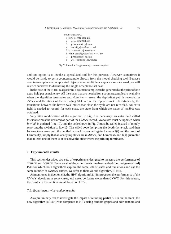
COUNTEREXAMPLE

1 for i := 0 to dtopdo2 p := dstack[i].pos3 print cstack[p].state4 cstack[p].lowlink := −15 p := cstack[p].lowsource6 while cstack[p].lowlink = −1 do7 print cstack[p].state8 p := cstack[p].lowsource

Fig. 7. A routine for generating counterexamples.

and one option is to invoke a specialized tool for this purpose. However, sometimes itwould be handy to get a counterexample directly from the model checking tool. Becausecounterexamples are complicated objects when multiple acceptance sets are used, we willrestrict ourselves to discussing the single acceptance set case.In the caseof theTCHECKalgorithm, a counterexample canbegenerated at the price of one

extra field percstackentry. All the states that are needed for a counterexample are availablewhen the algorithm terminates andviolation = TRUE: the depth-first path is recorded indstackand the states of the offending SCC are at the top ofcstack. Unfortunately, thetransitions between the brown SCC states that close the cycle are not recorded. An extrafield is needed to record, for each state, the state from which the value oflowlink wasobtained.Very little modification of the algorithm in Fig.3 is necessary: an extra field called

lowsourcemust be declared as part of theCStackrecord,lowsourcemust be updated whenlowlink is updated (line 19), and the code shown in Fig. 7 must be called instead of merelyreporting the violation in line 15. The added code first prints the depth-first stack, and thenfollows lowsourceuntil the depth-first stack is reached again. Lemma 1(i) and the proof ofLemma 3(b) imply that all accepting states are indstack, and Lemmas 6 and 1(h) guaranteethat at least one of them is at or above the state where the printing terminates.

7. Experimental results

This section describes two sets of experiments designed to measure the performance ofTCHECKandDCHECK. Because all of the experiments involve standard (i.e., not generalized)BAs for which both algorithms explore the same sets of states and transitions and use thesame number ofc/estackentries, we refer to them as one algorithm,CHECK.Asmentioned in Section 6.2, the HPY algorithm [21] improves on the performance of the

CVWY algorithm in some cases, and never performs worse than CVWY. For this reason,the results in this section are all based on HPY.

7.1. Experiments with random graphs

As a preliminary test to investigate the impact of retaining partial SCCs on the stack, thenew algorithm (CHECK) was compared to HPY using random graphs and both random and


actual LTL formulas. The procedure described in[30] was used to generate 360 randomformulas, another 94 formulas were selected from the literature (12 from [10], 27 from [28],55 from [8]), anda further 36were taken fromapersonal collectionof troublesome formulas.Also the negations of these formulas were added to the list, bringing the total to 980. Noattempt was made to remove duplicate LTL formulas. Each formula was converted to aBüchi automaton using theLTL2BA program [12], and the number of states in the resultingBüchi automata ranged from 1 to 177. Using another procedure from [30], 75 random 100-state graphs were generated. The graph generation algorithm selects one state as the rootand ensures that every other state is reachable from it.Every graph was checked against every LTL formula. Table 1 shows the outcome of

the comparison. The three major columns contain the results for the random formulas, thehuman-generated formulas and the combined set, respectively. The major rows divide theresults according to the connectedness of the graphs; each row describes 15 graphs that weregenerated with the same transition probability, while the last row contains the combinedresults for all 75 graphs. For each major row and column, the number in italics indicatesin how many cases violations were found. For both the new and the HPY algorithm threenumbers indicate the number of unique states reached, the number of transitions explored,and the maximum size ofcstack(for CHECK) or the procedural stack (for HPY), averagedover the instances of violations, and expressed as a percentage of the total number of statesor transitions in the product of the graph and the Büchi automaton. This means that everynumber in the last column is the sum of its counterparts in the first two columns, weightedwith the number of violations.For example, the 720 random formulas (360 randomly generated and negated) were

checked against the 15 random graphs with a transition probability of 0.001. Of the 10 800products, 7133 contained violations.CHECK reported a violation (there may be several ineach product) after exploring on average 8.71% of the states and 6.74% of the transitionsof the product. During the search,cstackcontained a maximum of 6.83% of the stateson average. In contrast, the HPY algorithm reports a violation after exploring on average41.59% of the states and 30.04% of the transitions, and during the search its stack containedat most 37.79% of the states on average. (This includes the usual depth-first and the nesteddepth-first search stacks.) All in all, violations were found in 54 068 of the 73 500 productsinvestigated.The product automaton explored by the HPY algorithm may, in some sense, have up to

twice as many states and transitions as that explored by the new algorithm. Each stateshasa depth-first version〈s,0〉 and, if the state is reachable from an accepting state, a nesteddepth-first version〈s,1〉, and the same holds for the transitions. However, in our opinionthe figures as reported in the table give a good idea of the memory consumption of thealgorithms (indicated by the percentage of states and maximum stack size) and the timeconsumption (indicated by the percentage of transitions). When states are stored explicitly,it is possible to represent the nested version of each state by storing only one additional bitper state. In this case, the HPY figures for states may be divided by two before reading thetable, to get a lower estimate.The results clearly demonstrate that on average the new algorithm is faster (i.e., explores

fewer transitions) and more memory efficient (i.e., stores fewer visited states and uses lessstack space) than HPY,for the formulas and random graphs investigated. From experience


Table 1Comparison of theTCHECK and HPY algorithms for random graphs

Edge Random formulas Human-generated Combinedprob. Algo. formulas

0.001 7133 2949 10082CHECK 8.71 6.74 6.83 9.68 7.30 7.86 8.99 6.91 7.13HPY 41.59 30.04 37.79 36.29 25.89 31.70 40.04 28.82 36.01

0.01 7267 3039 10306CHECK 6.15 4.08 4.67 6.40 3.85 5.50 6.22 4.01 4.91HPY 24.95 14.63 21.42 23.52 13.21 19.92 24.53 14.21 20.97

0.1 7832 3131 10963CHECK 6.38 2.90 4.10 5.69 1.62 4.74 6.19 2.53 4.28HPY 78.10 32.11 72.07 64.28 23.91 57.70 74.15 29.77 67.96

0.5 8150 3168 11318CHECK 6.02 2.16 3.20 5.11 1.08 3.89 5.76 1.86 3.40HPY 92.51 47.51 84.66 80.45 35.13 70.64 89.13 44.05 80.73

0.9 8222 3177 11399CHECK 6.04 2.06 3.00 5.57 1.11 4.30 5.91 1.80 3.36HPY 88.88 47.19 80.50 81.76 35.88 71.24 86.89 44.04 77.92

All 38604 15464 54068CHECK 6.62 3.50 4.29 6.45 2.93 5.22 6.57 3.33 4.55HPY 66.69 34.90 60.65 57.83 26.94 50.75 64.15 32.62 57.82

we know that results on random graphs can be misleading; results for actual models andformulas are discussed below.

7.2. Experiments with actual models

We have implemented a model of the echo algorithm with extinction for electing leadersin an arbitrary network, as described in[31, Chapter 7]. Three variations of the model wereinvestigated:• Variation 1: After a leader has been elected and acknowledged by the other nodes, theleader abdicates and a new election is held. The same node wins every election.

• Variation2: A leader is elected and abdicates, as in Variation 1. However, a counter keepstrack of the previous leader and gives each node a turn to win the election.

• Variation 3: As in Variation 2, each node gets a turn to become leader. However, onenode contains an error that disrupts the cycle of elections.

Each of the variations was modelled with theSPIN system and its state space, reducedwith partial orders, was converted to a graph for input by our cycle detection algorithms.This is not the way the algorithms would be used in practice—cycle detection normallyruns concurrently with the generation of the state space—but it facilitated making theexperiments without having to implement the new algorithm inSPIN.


Table 2Results of checking property� for leader election in an arbitrary network

� Product CHECK HPY

Variation1: 25 714states, 32 528transitionsA 51053 96406 51053 96406 14097 51053 128342 14097B × 51849 100521 422 436 422 1159 1227 1151C 12081 15198 12081 15198 199 12081 30395 199D 51053 96406 51053 96406 14097 51053 128342 14097E × 25714 32529 389 390 389 642 657 639F 51053 96406 51053 96406 14097 51053 128342 14097G 25714 32529 25714 32529 14097 25714 32529 14097H × 53988 88553 610 624 610 19649 24417 1511I × 53988 88553 610 624 610 19649 24417 1511

Variation2: 51 964states, 65 701transitionsA × 104779 204228 26742 49909 13841 35786 87539 1472B × 105599 208455 886 900 886 3016 3168 3008C 12081 15198 12081 15198 199 12081 30395 199D 103541 195893 103541 195893 40347 103541 260986 40347E × 51964 65702 853 854 853 1570 1585 1567F 103541 194225 103541 194225 40347 103541 259318 40347G × 92140 118238 1122 1123 1122 1803 1805 1803H × 293914 552899 1567 1581 1567 56254 69736 4269I 132763 222806 132763 222806 40347 211890 377639 40347

Variation3: 40 158states, 51 115transitionsA × 81167 160470 904 906 904 2133 2222 2132B × 81987 164697 904 906 904 2133 2222 2132C 12081 15198 12081 15198 199 12081 30395 199D × 79929 152135 12777 16125 697 13239 31784 1159E × 40158 51116 697 698 697 1159 1161 1159F × 79929 150467 12777 16125 697 13239 31784 1159G × 66450 86258 903 904 903 1365 1367 1365H × 229269 435261 30917 57851 2009 142993 271769 2516I × 169793 312465 37798 63689 14688 150362 281812 2292

A ≡ ♦�(n U l0) n ≡ there is no leaderB ≡ ♦�(n U l3) lx ≡ processx is the leaderC ≡ ♦l0 L(x, y) ≡ lx ⇒ (lx U (n U ly ))D ≡ �♦l0E ≡ ♦l3F ≡ �(n ⇒ ♦l0) H ≡ ♦�((n ∨ l0 ∨ l1 ∨ l2) ∧ L(0,1) ∧ L(1,2) ∧ L(2,0))G ≡ �(n ∨ l0) I ≡ ♦�((n ∨ l0 ∨ l1 ∨ l2) ∧ L(0,2) ∧ L(1,0) ∧ L(2,1))

The results of our comparison are shown in Table2. The first column contains thenames of the formulas which are given explicitly below the table; a cross to the rightof the formula name indicates that a violation of the property was detected. The col-umn marked “Product” gives the number of states and transitions in the product automa-ton, and the columns marked “CHECK” and “HPY” give the number of states, transitionsand the maximum stack size for the new algorithm and for the HPY algorithm,respectively.


Fig. 8. A difficult case for the new algorithm.

The arbitrary network specified in the model variations comprises three nodes numbered0, 1, and 2. This explains why propertyE (“node 3 is eventually elected at least once”) isnot satisfied by any of the models. PropertiesA, C, D, F, andG deal with the election ofnode 0, and propertiesH andI say that, from some point onward, the elected leader followsthe cycles 0–1–2 and 0–2–1, respectively.In all cases, the numbers of states and transitions explored by the new algorithm are the

same as or less than those explored by HPY. In three cases, variation 1H and 1I and 2H,the new algorithm explores more than 30 times fewer states and transitions. In two cases,2A and 3I , the new algorithm requires more stack entries than the other algorithm. Whichalgorithmwins in these two cases depends on implementation details, but the new algorithmis clearly the overall winner.

8. Heuristics

It is not difficult to construct a scenario whereCHECK fares worse memory-wise than theCVWY algorithm. Consider the Büchi automaton and the systemS in Fig. 8. The producthas exactly the same shape asSexcept that the state marked� is accepting, and forms thesingle accepting cycle.Assuming that transitions are explored left-to-right, the CVWY algorithm detects the

accepting cycle after exploring the four states of the subgraph rooted at state�. Its stackreaches a maximum depth of four, and at the time of the detection its stack also containsfour states (three regular states and one nested-search state). TheCHECK algorithm, on theother hand, also explores the four states of the subgraph rooted at�, but, because they forman SCC rooted at the initial state, these states remain on the stack. At the time of detectingthe accepting cycle, the new algorithm’s stack contains all seven states of the product. Thesituation is even worse if the system contains two such subgraphs, as doesS′ in Fig. 8. Inthis case, CVWY explores the subgraphs at�0 and�1, but its stack reaches a maximumsize of only four.CHECKretains all states on the stack, so that it contains 11 states when theaccepting cycle is found.If only the transition leading to� were explored first, both algorithms would detect

the offending cycle after exploring just three states (plus an extra nested-search state for


Table 3Effect of heuristics on theCHECK algorithm

Random Human generatedHeuristic formulas formulas Combined

NONE 6.62 3.50 4.29 6.45 2.93 5.22 6.57 3.33 4.55+DEPTH 6.72 3.34 4.28 7.88 3.46 6.29 7.05 3.37 4.85−DEPTH 11.40 5.95 8.98 14.86 7.47 13.33 12.39 6.38 10.23+ACCEPT 13.04 6.82 10.15 16.47 8.16 14.71 14.02 7.20 11.46−ACCEPT 7.62 3.62 5.80 10.25 4.97 8.97 8.37 4.01 6.71+STAY 12.03 6.15 9.76 16.27 8.04 14.65 13.24 6.69 11.16−STAY 8.30 3.99 6.10 12.06 5.63 10.55 9.37 4.46 7.37+TRUE 9.03 4.39 6.58 12.91 5.95 11.03 10.14 4.83 7.85−TRUE 13.16 6.50 10.84 17.17 8.27 15.27 14.31 7.00 12.11

CVWY). This suggests the use of heuristics to guide the algorithms to detect acceptingcycles more quickly.Eight heuristics were investigated, and the results are shown in Table3. The meaning of

the three columns is the same as in Table 1, as is the meaning of the three numbers (states,transitions, maximum stack size) given per experiment. Only the performance of theCHECK

algorithm is described in the table, and the first line—which agrees with the lastCHECK lineof Table 1—shows the case where no heuristics are used.The following heuristics were investigated:+DEPTH (−DEPTH) selects those transitions

that lead to the deepest (shallowest) Büchi SCC first,+ACCEPT (−ACCEPT) selects thosetransitions thatmove closest to (furthest away from) an accepting state first,+STAY (−STAY)selects those transitions that stay within the same Büchi SCC first (last), and+TRUE(−TRUE) selects those transitions that are labelled with the formula “true” first (last). Ifthere are any ties between transitions, the order in which the transitions appear in the inputis followed.As the table shows, none of the heuristics performed better than using no heuristic at

all. This is disappointing, but it does not mean that heuristics do not work. Rather, theproblem might be that some heuristics work well for some Büchi automata, and poorlyfor others. Suggestions for heuristics search based on system transitions have been madein [17,23], and, more recently, in [9,34]. Both of the new algorithms presented in this papercan accommodate these suggestions.

9. Conclusions

We have presented two alternatives to the CVWY [3] and HPY [21] algorithms for cycledetection in on-the-fly verification with Büchi automata. The first one is from [13], and thesecond combines ideas from [5] and [13]. Both our algorithms report a violation as soon asan ordinary depth-first search has found every transition of any accepting cycle. Thus, theyare able to find errors quicker than CVWY and HPY, which need to start backtracking first.Also, they never investigate a state more than once, making them compatible with otherverification techniques that rely on depth-first search.


They sometimes require a lot of stack space, but our measurements indicate that thisdrawback is usually outweighed by their ability to detect errors quickly. One aspect inwhich the algorithms are inferior to CVWY/HPY is that they need to store some stackinformation in random accessmemory. Their performance degrades significantly comparedto CVWY/HPY if the stack grows so large that parts of it need to be moved to slow diskmemory. On the other hand, the new algorithms are compatible with bitstate hashing andrequire only a single bit whereas the CVWY/HPY algorithms require two.

Acknowledgements

The authors wish to thank Dragan Bošnacki for pointing out the reference to Dijkstra’sstrongly connected component algorithm. The work of J. Geldenhuys was funded by theTISE graduate school and by the Academy of Finland.

References

[1] A.V. Aho, J.E. Hopcroft, J.D. Ullman, The Design and Analysis of Computer Algorithms, Addison-Wesley,Reading, MA, 1974.

[2] K.A. Bartlett, R.A. Scantlebury, P.T. Wilkinson, A note on reliable full-duplex transmission over half-duplexlinks, Comm. ACM 12 (5) (1969) 260–261.

[3] C. Courcoubetis, M.Y. Vardi, P. Wolper, M. Yannakakis, Memory-efficient algorithms for the verification oftemporal properties, in: Proc. 2nd Internat. Conf. on Computer-Aided Verification (CAV’90), Lecture Notesin Computer Science, Vol. 531, Springer, Berlin, June 1990, pp. 233–242.

[4] C. Courcoubetis, M.Y. Vardi, P. Wolper, M. Yannakakis, Memory-efficient algorithms for the verification oftemporal properties, Formal Methods System Design 1 (2/3) (1992) 275–288.

[5] J.-M. Couvreur, On-the-fly verification of linear temporal logic, in: Proc.World Congress on FormalMethodsin theDevelopment ofComputingSystems (FM’99), LectureNotes inComputerScience,Vol. 1708,Springer,Berlin, September 1999, pp. 253–271.

[6] M. Daniele, F. Giunchiglia, M.Y. Vardi, Improved automata generation for linear time temporal logic, in:Proc. 11th Internat. Conf. on Computer-Aided Verification (CAV’99), Lecture Notes in Computer Science,Vol. 1633, Springer, Berlin, July 1999, pp. 249–260.

[7] E.W.Dijkstra, Finding themaximumstrong components in a directed graph (EWD376),May 1973, Publishedin: A Discipline of Programming, Prentice-Hall, EnglewoodCliffs, NJ, Chap. 25, 1976; in: SelectedWritingson Computing: A Personal Perspective, Springer, Berlin, 1982, pp. 22–30.

[8] M.B. Dwyer, G.S. Avrunin, J.C. Corbett, Property specification patterns for finite-state verification, in: Proc.2nd ACMWorkshop Formal Methods in Software Practice, March 1998, pp. 7–15.

[9] S. Edelkamp, S. Leue, A. Lluch Lafuente, Directed explicit-state model checking in the validationof communication protocols, Technical Report 161, Institut für Informatik, Albert-Ludwigs-UniversitätFreiburg, October 2001.

[10] K. Etessami, G.J. Holzmann, Optimizing Büchi automata, in: Proc. 11th Internat. Conf. on ConcurrencyTheory (CONCUR’00), Lecture Notes in Computer Science, Vol. 1877, Springer, Berlin, August 2000,pp. 154–167.

[11] P. Gastin, P. Moro, M. Zeitoun, Minimization of counterexamples inSPIN, in: Proc. 11th Internat.SPINWorkshop on Model Checking Software, Lecture Notes in Computer Science, Vol. 2989, Springer, Berlin,April 2004, pp. 92–108.

[12] P. Gastin, D. Oddoux, Fast LTL to Büchi automata translation, in: Proc. 13th Internat. Conf. on Computer-Aided Verification (CAV’01), Lecture Notes in Computer Science, Vol. 2102, Springer, Berlin, July 2001,pp. 53–65.


[13] J. Geldenhuys, A. Valmari, Tarjan’s algorithm makes on-the-fly LTL verification more efficient, in: Proc.10th Internat. Conf. on Tools and Algorithms for the Construction and Analysis of Systems (TACAS’04),Lecture Notes in Computer Science, Vol. 2988, Springer, Berlin, March–April 2004, pp. 205–219.

[14] R. Gerth, D. Peled, M.Y. Vardi, P. Wolper, Simple on-the-fly automatic verification of linear temporallogic, in: Proc. 15th IFIP Symp. on Protocol Specification, Testing, and Verification (PSTV’95), June 1995,pp. 3–18.

[15] P. Godefroid, Partial-order methods for the verification of concurrent systems, an approach to the state-explosion problem, Ph.D. Thesis, University of Liège, December 1994, also appeared as Lecture Notes inComputer Science, Vol. 1032, Springer, Berlin, 1996.

[16] P.Godefroid,G.J.Holzmann,On the verification of temporal properties, in: Proc. 13th IFIPSymp. onProtocolSpecification, Testing, and Verification (PSTV’93), May 1993, pp. 109–124.

[17] P. Godefroid, G.J. Holzmann, D. Pirottin, State space caching revisited, in: Proc. 4th Internat. Conf. onComputer-Aided Verification (CAV’92), Lecture Notes in Computer Science, Vol. 663, Springer, Berlin,June 1992, pp. 175–186, also appeared in Formal Methods in System Design 7(3) (1995) 227–241.

[18] A.Groce,W.C. Visser,What went wrong: explaining counterexamples, in: Proc. 10th Internat.SPINWorkshopon Model Checking Software, Lecture Notes in Computer Science, Vol. 2648, Springer, Berlin, May 2003,pp. 121–135.

[19] G.J. Holzmann, An improved reachability analysis technique, Software Practice Experience 18 (2) (1988)137–161.

[20] G.J. Holzmann, An analysis of bitstate hashing, Formal Methods System Design 13 (3) (1998) 287–307.[21] G.J. Holzmann, D. Peled, M. Yannakakis, On nested depth first search, in: Proc. 2ndSPINWorkshop, 1997,

pp. 23–32, held August 1996, DIMACS Series No. 2.[22] G.J. Holzmann, A. Puri, A minimized automaton representation of reachable states, Software Tools Tech.

Transfer 2 (3) (1999) 270–278.[23] F.J. Lin, P.M. Chu, M.T. Liu, Protocol verification using reachability analysis: the state space explosion

problem and relief strategies, Comput. Comm. Rev. 17 (5) (1987) 126–135.[24] E. Nuutila, E. Soisalon-Soininen, On finding the strongly connected components in a directed graph, Inform.

Process. Lett. 49 (1) (1994) 9–14.[25] D. Peled, All from one, one for all: on model checking using representatives, in: Proc. 5th Internat. Conf.

on Computer-Aided Verification (CAV’93), Lecture Notes in Computer Science, Vol. 697, Springer, Berlin,June 1993, pp. 409–423.

[26] K. Schneider, Improving automata generation for linear temporal logic by considering the automatonhierarchy, in: Proc. 8th Internat. Conf. on Logic for Programming, Artificial Intelligence, and Reasoning,Lecture Notes in Computer Science, Vol. 2250, Springer, Berlin, December 2001, pp. 39–54.

[27] M. Sharir, A strong-connectivity algorithm and its application in data flow analysis, Comput. Math. Appl. 7(1) (1981) 67–72.

[28] F. Somenzi, R. Bloem, Efficient Büchi automata from LTL formulae, in: Proc. 12th Internat. Conf. onComputer-Aided Verification (CAV’00), Lecture Notes in Computer Science, Vol. 1855, Springer, Berlin,June 2000, pp. 67–72.

[29] R.E. Tarjan, Depth-first search and linear graph algorithms, SIAM J. Comput. 1 (2) (1972) 146–160.[30] H. Tauriainen, A randomized testbench for algorithms translating linear temporal logic formulae into

Büchi automata, in: Proc. Workshop on Concurrency, Specifications, and Programming, September 1999,pp. 251–262.

[31] G. Tel, Introduction to Distributed Algorithms, second ed., Cambridge University Press, Cambridge, 2000.[32] A. Valmari, A stubborn attack on state explosion, Formal Methods System Design 1 (1) (1992) 297–322.[33] P. Wolper, M.Y. Vardi, A.P. Sistla, Reasoning about infinite computation paths, in: Proc. 24th IEEE Symp. on

the Foundations of Computer Science, IEEE Computer Society Press, Silver Springs, MD, November 1983,pp. 185–194.

[34] C.H. Yang, D.L. Dill, Validation with guided search of the state space, in: Proc. 35th Conf. on DesignAutomation, ACM Press, New York, June 1998, pp. 599–604.

more efficient on-the-fly ltl verification with tarjan's algorithm

Documents