moothing, splines and smoothing s their application in...

JOURNAL OF COMPUTATIONAL PHYSICS 78, 493-508 (1988)

moothing, Splines and Smoothing S Their Application in G~orn~gn~ti~rn

C. 6. CONSTABLE AND R. L. PARKER

Instirufe of Geophysics and Planetary Physics, Scripps Institution of Oceanography, University of California, San Diego, La Jolla, California 92093

Received August 11, 1987; revised January 4, 1988

We discuss the use of smoothing splines (SS) and least squares splines (LSS) in non- parametric regression on geomagnetic data. The distinction between smoothing splines and least squares splines is outlined, and it is suggested that in most cases the smoothing spline is a preferable function estimate. However, when large data sets are involved, the smoothing spline may require a prohibitive amount of computation; the alternative often put forward when moderate or heavy smoothing is desired is the least squares spline. This may not be capable of modeling the data adequately since the smoothness of the resulting function can be controlled only by the number and position of the knots. The computational efficiency of the least squares spline may be retained and its principal disadvantage overcome, by adding a penalty term in the square of the second derivative to the minimized functional. We call this modified form a penalized least squares spline, (denoted by PS throughout this work), and illustrate its use in the removal of secular trends in long observatory records of geomagnetic

field components. We may compare the effects of smoothing splines, least squares splines, and penalized least squares splines by treating them as equivalent variable-kernel smoothers. As Silvernzan has shown, the kernel associated with the smoothing spline is symmetric and is highly localized with small negative sidelobes. The kernel for the least squares spline with the same fit to the data has large oscillatory sidelobes that extend far from the central region; it can be asymmetric even in the middle of the interval. For large numbers of data the penalized least squares spline can achieve essentially identical performance to that of a smoothing sphne, but at a greatly reduced computational cost. The penalized sphne estimation technique has potential widespread applicability in the analysis of geomagnetic and paleomagnetic data. It may be used for the removal of long term trends in data, when either the trend cr the residual is of interest. la 1988 Academic Press, Inc.

1. INTRODUCTION

Hn this paper we discuss a practical problem that frequently arises in the analysis of geomagnetic data, namely fitting a smooth curve of unknown parametric fo a time series of observations. The goal may be to interpolate the data ~rovid.jng a means of studying long term trends or to remove a trend and look at the rerna~~~~~ part of the signal. The approach that we advocate is that of using cubic srnoot~~~~ splines to estimate the unknown function, i.e., finding the smoothest twice continuously differentiable function fitting the observations to a specified tolerance. The use of smoothing splines (SS) has particular merit in cases where one is dialing

493 00X-9991/88 $3.00

Copyright 0 1988 by Academic Press. Inc. Al1 rights of reproduction in any form reserved.

494 CONSTABLE AND PARKER

with irregularly spaced noisy data; then the standard filtering techniques used in time series analysis become somewhat awkward to implement. SS have been used in the analysis of historical geomagnetic and paleomagnetic data (see, e.g., Clark and Thompson [a]; Parker and Denham [7]; Malin and Bullard [6]) for the purposes of obtaining smooth curves from noisy data records. Here, we discuss the possibility of using them in the study of ionospheric signals in geomagnetic observatory data, for which we found it necessary to remove the long period secular trends associated with variations in the internal part of the geomagnetic field. Many of the records with which we were dealing extended back further than the available secular variation models obtained from global geomagnetic data, necessitating a means of estimating the variation directly from data at a single site. The data used were hourly mean values of the geomagnetic field, so that for records 30 years long the computational problem of finding the SS is considerable. One approach to reducing the computational task is to use least squares splines (denoted here by LSS) to estimate the function (e.g., [12, 131). Algorithms for this type of estimation (and also for SS) are widely available in the standard mathematical software libraries such as IMSL and SLATEC. This method is an example of collocation; the only control over the smoothness of the resulting function comes from the choice of

0 100 200 300

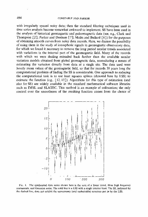
FIG. 1. The synthesized data series shown here is the sum of a linear trend, three high frequency cosinusoids, and Gaussian noise. The solid line is a LSS with a single interior knot. The SS, indicated by the dashed line, does not exhibit the unnecessary (and undesirable) structure put in by the LSS.

SMOOTHING, SPLINES, AND SMOOTHING SPLINES

number and positions of the knots and the connection points for the sphne basis functions (which are piecewise cubic polynomials).

There are situations in which SS may be judged too expensive and LSS cannot model the data adequately. This is perhaps best illustrated by an example where LSS fails to perform adequately. Figure 1 shows a synthetic data series consistin the sum of a linear trend, three high frequency cosinusoids, and Gaussian noise. The solid curved line is a LSS with a single interior knot, and does a very p of recovering the linear trend. The SS, shown dashed, on the other hand satisfactory job, because of the additional smoothing constraint imp minimizing tbe second derivative. This has led us to develop the ~~oced~~c described here, which we shall refer to as penalized least squares splines (and abbreviate by PS), and provides an excellent approximation to the SS at a greatly reduced computational cost.

In the next section we outline the distinctions between these t PS, and SS. Then we present an algorithm for the solution to th last section illustrates the properties of the three splines when t kernel smoothers or filters and shows why the LSS performs so circumstances.

2. CUBIC SPLINE SMOOTHING

Let us suppose that we have N observations yi, i= 1, . . . . N at points xi, fro which we wish to determine a function f(x), whose parametric form is not known, and that

Yi = f(Xi) + 8,

We assume that x1 <x2 < . . . < xN and that Q are random, uncorrelated errors wit zero mean and variance 0:. The appoach that we favor is the following: we seek the smoothest possible function in the class C*[x, , xN] (the class of twice c~~ti~~~~s~y differentiable functions on the closed interval x1, xN) fitting the observa specified tolerance. The misfit to the data is measured by the weight squared discrepancies:

and the roughness, which is to be minimized, is just the square of the two-nor ” of the second derivative:

s xN [lag(x)]” dx. Xl


It is well known [9, S] that the solution to this problem is the minimizer, fs(x), over functions f E C2[xI, xN] of the functional

where A > 0 is a smoothing parameter controlling the trade-off between smoothness of f and goodness of fit to the data; 2 is not specified directly, but must be discovered by finding the minimizer fs with the correct misfit. The functions f, are called the smoothing spline (here abbreviated to SS) estimators of the data. Upon application of calculus of variations the following property of the SS is immediately apparent: for every choice of A > 0, f, is a separate cubic polynomial within each interval [xi, xi+ i]. In the terminology of the spline literature, the transition points Xi between one polynomial and the next are called the “knots” of the spline; for f, the knots are identical to the points where the data are measured, but in general this need not be the case.

When heavy smoothing is appropriate we often find a very simple-looking minimizer f,, but that function requires a seemingly excessive number of parameters to specify it: there are almost as many cubic polynomials (N- 1) as original data (N). Furthermore, when N is very large the computational cost of finding the optimally smooth curve in this way may be judged too high. It seems obvious that a smooth curve can be quite accurately represented by a much smaller number of parameters than the number required to match every wiggle of the uncorrelated random component of the measurements. This idea corresponds to LSS: here the number of knots is reduced to a small fraction of the number of data and least squares regression is performed in the B-spline basis fuctions associated with these knots [ 1, Chap. XIV]. The smoothness of the resulting function is controlled by the number and position of the knots instead of by means of a continuous parameter. There is no explicit roughness penalty in the minimized functional, corresponding to the second term in (1). In our experience, LSS have a number of drawbacks. The question of exactly how many knots should be used and their optimum location is a delicate problem, not yet satisfactorily solved. Furthermore, we have discovered practical situations in which it is impossible to enforce a high enough degree of smoothness, even with very small numbers of knots (e.g., the example of Fig. 1). When the action of the LSS is viewed as a kernel operator, the kernel is found to have excessive subsidiary peaks and asymmetry, properties quite undesirable in a good smoothing representation of the original data.

We present here a modification of the LSS technique that overcomes its dis- advantages while preserving, in large measure, its computational economy and descriptive parsimony. We return to the minimization of (l), but instead of minimizing over the whole function space C2[x,, x,], we restrict attention to a subspace spanned by a collection of B-splines defined on a set of equally spaced knots. The idea is to use only as many knots as necessary to give a reasonable approximation to the SS f,; in the case of strong smoothing this will be a tiny

SMOOTHING, SPLINES, AND SMOOTHING SPLINES 7

fraction of N. In the next section we present a numerical implementation of this penalized least squares spline (PS) problem, taking advantage of the banded ~at~rc of the resulting matrices. We show that after an initial “least squares” phase of computation in which all the data are involved, all further calculations (for example, those to select the proper value of A) can be performed on matrices with sizes governed by the number of knots. Also, it is possible at all times IS keep computer memory requirements to the order of L2, where L is the number of B-splines used. In Section 3 by means of Silverman’s [lo] asymptotic theory we are able to check the adequacy of our approximation to the optimally smooth f,: if the number of knots in a preliminary computation is too small the resulting curve at a specified level of misfit will be too rough and then it is necessary to repeat calculation with more knots so as to approach the desired smoothness. compare SS, LSS, and PS regarded as kernel smoothers and illustrate some of undesirable attributes of the ordinary LSS solution. The results show that, w large numbers of data are involved, the PS is a highly satisfactory a~t~~~ative to the SS.

3. SOLUTION TO THE PENALIZED LEAST SQUARES SPLINE PROBLEM

The cubic splines may be defined for our purposes as the set of functions in C2[c1, 5,] comprised of cubic polynomials on the intervals [tl, t2], [t2, t3],..., [tt_ I, tL J. The points <I < t2 < . . . < & are the knots of the splines. The B-s constitute a basis for rL, the space of cubic splines (see [ 1, Chap. IX]). As known, each element of the B-spline basis consists of a nonnegative functio with support [<j-,, ci+*] composed of cubic polynomial sections between t knots with continuity of the function and its first two derivatives at the knots, so that b, E C 2 [ 5 r, {J. A consequence of the continuity requirements is that, provi j>2, 6j(5j-,)=a,bj(tj_,)=a2bj(5,j-*)=Oand similarly at [j+Z. Ifthe knots Siam chosen to coincide with the measurement points xi the optimal SS solution ,i’, can be expanded in the B-spline basis. But, as we remarked in the introduction, our intent is to use a much sparser set of knot points upon which to erect a representation of the smooth function:

where L < N. We substitute the B-spline expansion into (1) and seek the minimizes over real aj of the function F:

Here we have assumed a simplified random component with identical variances of,


it is an easy matter to include the proper weighting if they are different but we have treated the special case to avoid unnecessarily cluttering up the notation. We introduce matrix notation with vectors and arrays having the following meanings: the matrix BE M(N x L), the space of N by L matrices, has elements B, = bj(xj); y E RN is the vector of data values; HE M(L x L) is a matrix of inner products of second derivatives of B-splines:

Hjk = s xN @,(x) i?&(x) dx. x1

The elements of Hare readily obtained in closed form and are particularly simple if the knots are evenly spaced in [xi, xN] as we shall assume from now on. In matrix notation (2) may be written

F= I/y-B~oll)~+la~H~~, (3)

where (/ . II is the Euclidean norm. Straightforward differentiation yields the following equation for CI~ E RL, the F-minimizing vector of expansion coefficients for fixed 1:

(BTB + AH) a, = BTy. (4)

Although the matrix on the left of (4) is only Lx L and therefore smaller than the one needed for the full SS solution, it runs the risk of poor conditioning because of its close connection to the normal equations (obtained in the limit as i tends to zero). We develop a procedure that avoids the unnecessary numerical instability associated with the normal equations by solving a related system through QR factorization.

The first term in (3) can be written as

where R E M(L x L) is an upper triangular matrix, the upper square portion of the right factor in the QR decompositions of B; y1 E lRL is the upper part of the rotated data vector y and yZ E RNPL the lower part of that vector. This is just the result of the application of the standard QR process to the first term of (3). As described in great detail by Lawson and Hanson [S, Chap. 271, the reduction to upper triangular form of B and the rotation of y can be performed very efficiently because B is banded; this is a direct result of the property that the support of b)(x) is [tie*, <j+2]. Furthermore, it is unnecessary to hold all of B or y in the computer memory at one time since blocks of data may be brought from the disk and condensed to upper triangular form in a sequence of operations. The Householder triangularization of B in its banded form takes between about 25N and 50N operations. The actual count depends on the size of the data blocks, the least efficient result occurring when data are added to the system one row at a time. Because the value of /z required to obtain the desired tolerance is not known at the


outset, it is always necessary to solve the system several times with deferent Q

but the bulk of the numerical work is over once this least s accomplished.

Since the term /( yZ/12 is unaffected by variations in a (it is t the best-fitting spline to the data), the function to be rniu~rn~z

F,= (jy,-Ra(/2+?a (51

If we can rewrite (5) as the sum of two terms, each of which is the square of a norm, we can continue to take advantage of the superior stability of position for the solution of the minimization problem. In order to proc a kind of Cholesky or square root factorization of the roughness pen&y matrix H, but this is not quite straightforward because H is of rank L - 2; this follows from the fact that a constant function and a linearly varying one are both in the sp rL, but the associated roughness aTHa vanishes in both cases. To solve problem we transform the vector of unknown coefficients to another vector a E RL as follows. Let

where

where I’ E M(L x L - 2) is an L. - 2 x L - 2 unit matrix a eve two rows of zeroes, and v19 u2 E RL are given by

v,=(L-1, L-2,...,O)[L(L-1)(2L-1)/6]-“”

v2 = (1, 1, ..~) 1) L-“2

so that /Iv1 // = I/vZ// = 1 and the matrix V is upper right triangular. Notice also t NV, = Hv, = 0 because v1 is the coefficient vector associated with a linearly vary function in an evenly distributed B-spline basis, and v2 is associated with a constant function. In terms of a the roughness functional becomes

aTHa= aTVTHVa,

where the matrix VTHV is composed of a positive definite, symmetric top left corner, which we shall call fi E M(L - 2 x L - 2), and a lowe border of zeros. Suppose I? has the Cholesky factorization 8= f~ M(L - 2 x L - 2) is lower triangular; then the roughness is

where JE M(L - 2 x L) is the Cholesky factor 3 with two co~~m¶s of zeros at the right.


Returning to (5) we may now write the function to be minimized as

(6)

which is just an ordinary, overdetermined least squares problem as we required. Since (6) must be minimized a number of times with different values of I it pays to make the solution of this part of the problem efficient also. Notice that both R and V are in upper triangular form, so their product RV is also upper triangular; J is in that form too. Consider reordering the rows of coefficient matrix by interleaving rows of RV with those of J so that in the reordered array everything in column j below row 2j is zero; the same reordering must be done on the vector, of course. When the QR decomposition of the reordered system is performed, there is no need to treat the already zero, lower left portion of the coefficient matrix; this reduces the usual operations count for the QR minimization of about 5L3/3 to only L3/3, a worthwhile improvement of a factor of five.

In practice the value of 1 which will yield the required tolerance S2 is not known a priori and must be found using an iterative procedure. The squared misfit for a given value of il is

For computational purposes this may be written as

The first and third terms in this expression are obtained during the solution of Eq. (6) and the initial QR decomposition of the B matrix, respectively. The second term is the part of the misfit obtained from the solution of (6) which arises from the roughness misfit and thus contributes nothing to the data misfit and must therefore be subtracted off.

In addition to possessing a lower bound of Sk,, = (/yz)12, the tolerance function is bounded above in the limit as ;1+ cx). Then the roughness of the resulting function is penalized to the maximum possible extent and the best-fitting straight line (in the least squares sense) will be obtained. We make use of this upper bound in the iterative procedure used to find the value of ;1 corresponding to the desired misfit. The value of s,&, can readily be found by performing the least squares tit to the straight line part of the spline, i.e., to vi and v2. Once the initial QR decomposition for B has been performed this is a straightforward QR solution to the Lx 2 system of equations


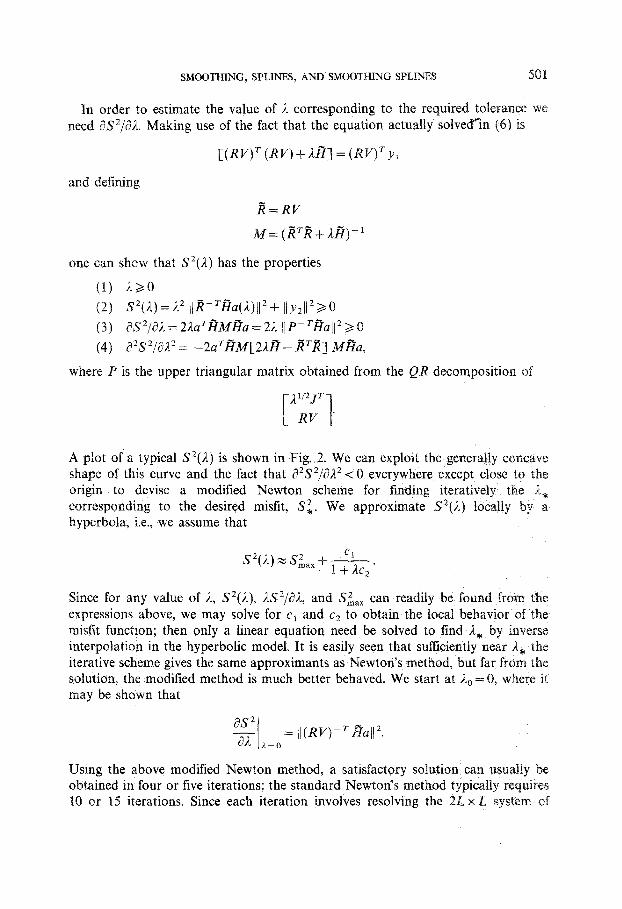
In order to estimate the value of ;1 corresponding to the required tolerance we need dS2/a/Z. Making use of the fact that the equation actually solved”in (6) is

[(RV)T (RV) + a.B] = (Rv)Ty,

and defining

i?=RV

M=(RTR+aWy

one can show that S’(A) has the properties

(4) aas0 (2) s2(a)=a2 llR-‘iTa(n)ll*+ lly*1/%l (3) as”/an=2naTfiM~a=221 ~~P-TRu~~230 (4) a?P/aP = -2aTfh4[2AA- iiTii] kfi;~~

where P is the upper triangular matrix obtained from tbe QR decomposition of

3 I/~JT

i” 1 RV

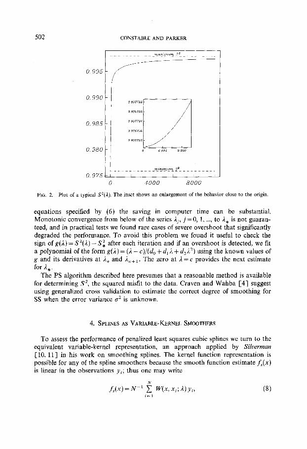
A plot of a typical S2(A) is shown in Fig. 2. We can exploit the generally concave shape of this curve and the fact that a2S2/dA2 < 0 everywhere except close to the origin to devise a modified Newton scheme for fmding iteratively the ,A, corresponding to the desired misfit, S:. We approximate S*(d) locally by a hyperbola, i.e., we assume that

S2@) = s;,, -I- &. 2

Since for any value of A, S”(A), AS*/aA, and S&, can readily be found from the expressions above, we may solve for cr and c2 to obtain the local behavior of the misfit function; then only a linear equation need be solved to find 1* interpolation in the hyperbolic model. It is easily seen that suf%ziently n iterative scheme gives the same approximants as Newton’s method, but solution, the modified method is much better behaved. We start at A0 = 0, where it may be shown that

as2 an i.=.

= il(RV)pT&ji2.

Using the above modified Newton method, a satisfactory solution can usually be obtained in four or five iterations; the standard Newton’s method typically requires 10 or I.5 iterations. Since each iteration involves resolving the 2L x L system of


0.995

0.990

0.985

0.980

0.975 c

0 4000 8000

FIG. 2. Plot of a typical s2(n). The inset shows an enlargement of the behavior close to the origin.

equations specified by (6) the saving in computer time can be substantial. Monotonic convergence from below of the series Aj, j= 0, 1, ,.., to A* is not guaran- teed, and in practical tests we found rare cases of severe overshoot that significantly degraded the performance. To avoid this problem we found it useful to check the sign of g(l) = A’“(A) - Si after each iteration and if an overshoot is detected, we tit a polynomial of the form g(A) = (A - c)/(d,, + d, A + &,A*) using the known values of g and its derivatives at A, and 1, + r. The zero at Iz = c provides the next estimate for A*.

The PS algorithm described here presumes that a reasonable method is available for determining S*, the squared misfit to the data. Craven and Wahba [4] suggest using generalized cross validation to estimate the correct degree of smoothing for SS when the error variance G* is unknown.

4. SPLINES AS VARIABLE-KERNEL SMOOTHERS

To assess the performance of penalized least squares cubic splines we turn to the equivalent variable-kernel representation, an approach applied by Silverman [lo, 111 in his work on smoothing splines. The kernel function representation is possible for any of the spline smoothers because the smooth function estimate f,(x) is linear in the observations yi; thus one may write

(8) i= 1


where xi, i= 1, . . . . N are the data sampling positions as before which fo coincide with the knot positions, ti. The weight function W(x, xi; ,I) shows data are averaged together to obtain the smoothed function estimate at a regard the weight function generated by the SS as the optimal one, and the to which the PS can reproduce that behavior will be taken as the m success. Obviously for the purposes of practical comparison we cannot a compute the true W for the SS; fortunately, the important properties of t function can be obtained without resorting to any heavy computations at ah.

Let the knot points have local density d(t) so that the proportion of ri in an interval of size d[ near 5 is approximately 4(c) d[. Then Silverman [ll] gives the asymptotic form of the weight function

W(x, 5; jl) = where K(u) is the kernel function

K(u)=iexp ( 1

-5 sin\-+: f’ ’ )

and the local averaging length scale or bandwidt

h(5) = A1’“qqlp4.

Numerically h(t) is a somewhat deceptive measure of the length scale over w the averaging kernel acts because it is too narrow. The distance from the ventral peak to the first zero of K(U) is (3~ ,/‘?/4)h x 3.332h. Silverman’s a~~roxirnati~~ for W(x, 5; 1) holds provided x is not too close to the edge of the interval Lx,) xN is not too large or too small, and N is sufficiently large. Equation (9) is not v near the boundaries of [x1, xN] but Silverman [lo] describes a rnodi~~at~o~ to account for this, under the same restrictions on N and a as before. He shows that these asymptotic forms agree well with the exact weight functions obtained for SS and we shall assume that this is true for all the cases of interest to us.

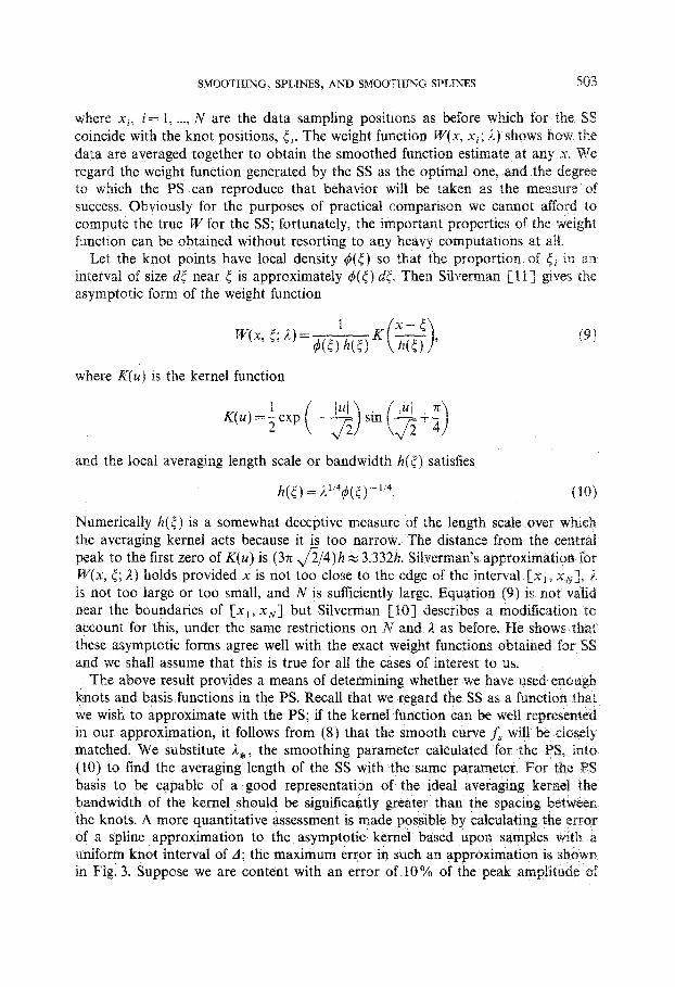
The above result provides a means of determining whether we have used e~o~~b knots and basis functions in the PS. Recall that we regard the SS as a function that we wish to approximate with the PS; if the kernel function can be well r~~~ese~ted in our approximation, it follows from (8) that the smooth curve f, will be eloseily matched. We substitute A,, the smoothing parameter calculated for the PS, i (10) to find the averaging length of the SS with the same parameter. For the basis to be capable of a good representation of the ideal averaging kernel bandwidth of the kernel should be significantly greater than the spacing between the knots. A more quantitative assessment is made possible by calculating the error of a spline approximation to the asymptotic kernel based upon samples wit uniform knot interval of d; the maximum error in such an approximation is in Fig. 3. Suppose we are content with an error of 10% of the peak arnpht


0. 1.0 2.0 3.0 Normalized knot spacing A/h

FIG. 3. Maximum error in the approximation of the asymptotic kernel K(U) by a cubic spline Kd based upon even knot spacing A.

K(U); then A/h must be less than 1.65, which corresponds to about four knot intervals under the central positive peak. Thus when 1.65h < A we expect the approximation to be poor. Conversely, we assert, when the knot interval is smaller than this, we will obtain a close correspondence between the ideal weight function and the true one. In the event that too few basis functions have been used for the PS, 1, will be smaller than the 1 for the true SS and thus the bandwidth of the resulting smoother will be underestimated.

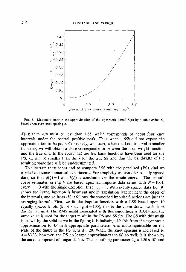
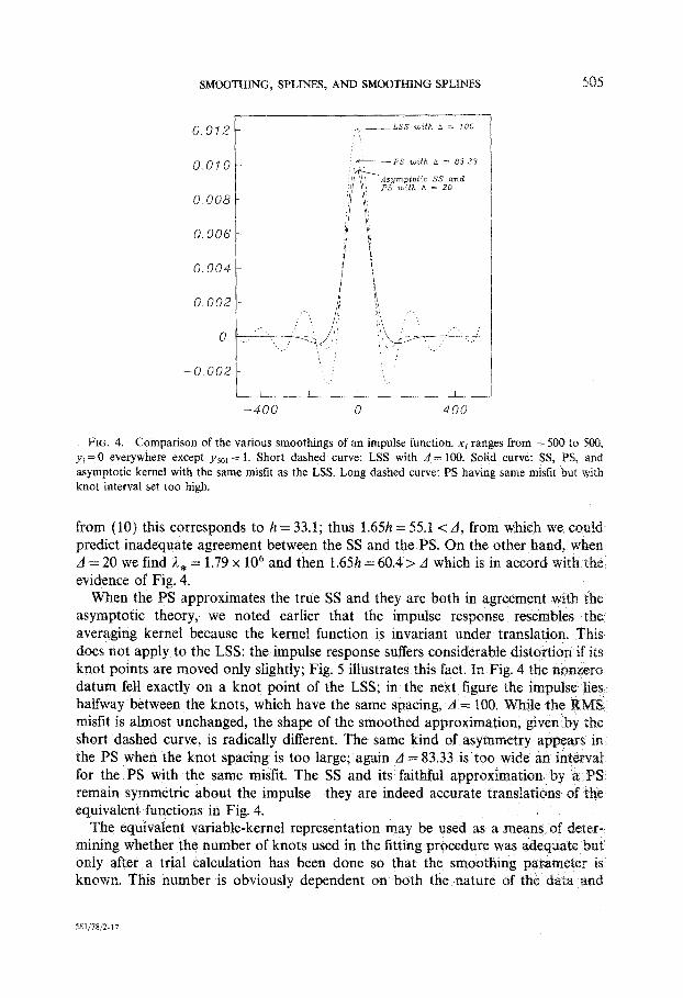
To illustrate these ideas and to compare LSS with the penalized (PS) kind we carried out some numerical experiments. For simplicity we consider equally spaced data, so that b(r) = 1 and h(t) is constant over the whole interval. The smooth curve estimates in Fig. 4 are based upon an impulse data series with N= 1001; every yi = 0 with the single exception that ysol = 1. With evenly spaced data Eq. (9) shows the kernel function is invariant under translation (except near the edges of the interval), and so from (8) it follows the smoothed impulse functions are just the averaging kernels. First, we lit the impulse function with a LSS based upon 10 equally spaced knots (knot spacing A = 100); this is the curve drawn with short dashes in Fig. 4. The RMS misfit associated with this smoothing is 0.0314 and the same value is used for the target misfit in the PS and SS fits. The SS with this misfit is shown by the solid curve in the figure; it is indistinguishable from the asymptotic approximation to W with appropriate parameters. Also indistinguishable on the scale of the figure is the PS with A = 20. When the knot spacing is increased to A = 83.33, however, the PS no longer approximates the SS so well; it is shown by the curve composed of longer dashes. The smoothing parameter 1, = 1.20 x lo6 and


0.006

-0.002 t

FIG. 4. Comparison of the various smoothings of an impulse function. xi ranges from - 500 to 500, yi=O everywhere except ysol = 1. Short dashed curve: LSS with d = 100. Solid curve: SS, PS, and asymptotic kernel with the same misfit as the LSS. Long dashed curve: PS having same misfit but with knot interval set too high.

from (LO) this corresponds to h = 33.1; thus 1.65h = 55.1 < .4, from which we coul predict inadequate agreement between the SS and the PS. On the other hand, when A = 20 we find A, = 1.79 x lo6 and then 1.6Sh = 60.4 > A which is in accord with the evidence of Fig. 4.

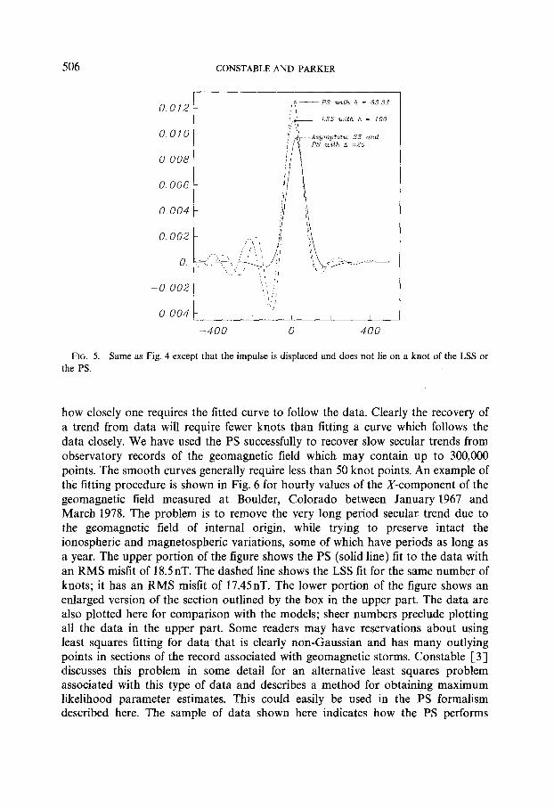
When the PS approximates the true SS and they are both in agreement with the asymptotic theory, we noted earlier that the impulse response resembles the averaging kernel because the kernel function is invariant under translation. This does not apply to the LSS: the impulse response suffers considerable distortion if its knot points are moved only slightly; Fig. 5 illustrates this fact. In Fig. 4 the nonzero datum fell exactly on a knot point of the LSS; in the next figure the impulse lies halfway between the knots, which have the same spacing, A = 100. While the R misfit is almost unchanged, the shape of the smoothed approximation, given by short dashed curve, is radically different. The same kind of asymmetry appears in the PS when the knot spacing is too large; again A = 83.33 is too wide an inter for the PS with the same misfit. The SS and its faithful approximation by a remain symmetric about the impulse-they are indeed accurate translations of the equivalent functions in Fig. 4.

The equivalent variable-kernel representation may be used as a means of mining whether the number of knots used in the fitting procedure was adequa only after a trial calculation has been done so that the smoothing parameter ’ known. This number is obviously dependent on both the nature of the data a


0.012

0.010

0.008

0.006

0.004

0.002

0.

-400 0 400

FIG. 5. Same as Fig. 4 except that the impulse is displaced and does not lie on a knot of the LSS or the PS.

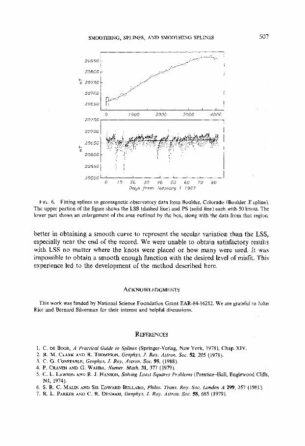
how closely one requires the fitted curve to follow the data. Clearly the recovery of a trend from data will require fewer knots than fitting a curve which follows the data closely. We have used the PS successfully to recover slow secular trends from observatory records of the geomagnetic field which may contain up to 300,000 points. The smooth curves generally require less than 50 knot points. An example of the fitting procedure is shown in Fig. 6 for hourly values of the X-component of the geomagnetic field measured at Boulder, Colorado between January 1967 and March 1978. The problem is to remove the very long period secular trend due to the geomagnetic field of internal origin, while trying to preserve intact the ionospheric and magnetospheric variations, some of which have periods as long as a year. The upper portion of the figure shows the PS (solid line) tit to the data with an RMS misfit of 18.5nT. The dashed line shows the LSS fit for the same number of knots; it has an RMS misfit of 17.45nT. The lower portion of the figure shows an enlarged version of the section outlined by the box in the upper part. The data are also plotted here for comparison with the models; sheer numbers preclude plotting all the data in the upper part. Some readers may have reservations about using least squares fitting for data that is clearly non-Gaussian and has many outlying points in sections of the record associated with geomagnetic storms. Constable [3] discusses this problem in some detail for an alternative least squares problem associated with this type of data and describes a method for obtaining maximum likelihood parameter estimates. This could easily be used in the PS formalism described here. The sample of data shown here indicates how the PS performs


20800 t h F: 20750

t 20700

20650 t

20650 h F:

20600

20550 : i

205-00~ I / I I

0 10 20 30 40 50 60 70 80 Days from January I 1967

FIG. 6. Fitting splines to geomagnetic observatory data from Boulder, Colorado (Boulder X sphne). The upper portion of the figure shows the LSS (dashed line) and PS (solid line) each ,with 50 knots. The lower part shows an enlargement of the area outlined by the box, along with the data from that region.

better in obtaining a smooth curve to represent the secular variation than the LSS, especially near the end of the record. We were unable to obtain satisfactory resuhs with LSS no matter where the knots were placed or how many were used. It was impossible to obtain a smooth enough function with the desired level of misfit. experience led to the development of the method described here.

ACKNOWLEDGMENTS

This work was funded by National Science Foundation Grant EAR-84-16212. We are grateful to John Rice and Bernard Silverman for their interest and helpful discussions.

REFERENCES

I. C. DE BOOR, A Practical Guide to Splines (Springer-Verlag, New York, 1978), Chap. XIV. 2. R. M. CLARK AND R. THOMPSON, Geophys. J. Roy. Astron. Sot. 52, 205 (1978). 3. C. G. CONSTABLE, Geophys. J. Roy. Astron. Sot. 95, (1988). 4. P. CRAVEN AND G. WAHBA, Numer. Math. 31, 371 (1979). 5. C. L. LAWSON AND R. J. HANSON, Solving Least Squares Problems (Prentice-Hall, Englewood Cliffs,

NJ, 1974). 6. S. R. C. MALIN AND SIR EDWARD BULLARD, Philos. Trans. Roy. Sot. London A 299, 357 (1981). 7. R. L. PARKER AND C. R. DENHAM, Geophys. .I. Roy. Astron. Sot. ~58, 685 (1979).


8. C. REINSCH, Numer. Math. 10, 177 (1967). 9. I. J. SCHOENBERG, Proc. Natl. Acad. Sci. USA 52, 947 (1964).

10. B. W. SILVERMAN, Ann. Stat. 12, No. 3, 898 (1984). 11. B. W. SILVERMAN, J. Roy. Stat. Sot. B 47, 1 (1985). 12. R. THOMPSON AND R. M. CLARK, Phys. Earth Planet. Inter. 27, 1 (1981). 13. R. THOMPSON AND D. R. BARRACLOUGH, J. Geomagn. Geolectr. 34, 245 (1982).

moothing, splines and smoothing s their application in...

Documents