Monte Carlo Methods

Guojin ChenChristopher Cprek Chris Rambicure

Monte Carlo Methods

• 1. Introduction • 2. History • 3. Examples

Introduction

• Monte Carlo methods are stochastic techniques.

• Monte Carlo method is very general. • We can find MC methods used in

everything from economics to nuclear physics to regulating the flow of traffic.

Introduction

• Nuclear reactor design• Quantum chromodynamics• Radiation cancer therapy• Traffic flow• Stellar evolution• Econometrics• Dow-Jones forecasting• Oil well exploration• VLSI design

Introduction

• A Monte Carlo method can be loosely described as a statistical method used in simulation of data.

• And a simulation is defined to be a method that utilizes sequences of random numbers as data.

Introduction (cont.)

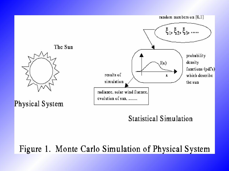
• The Monte Carlo method provides approximate solutions to a variety of mathematical problems by performing statistical sampling experiments on a computer.

• The method applies to problems with no probabilistic content as well as to those with inherent probabilistic structure.

Major Components

• Probability distribution function • Random number generator • Sampling rule• Scoring/Tallying

Major Components (cont.)

• Error estimation• Variance Reduction techniques• Parallelization/Vectorization

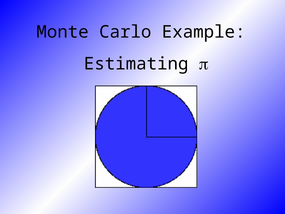
Monte Carlo Example:

Estimating

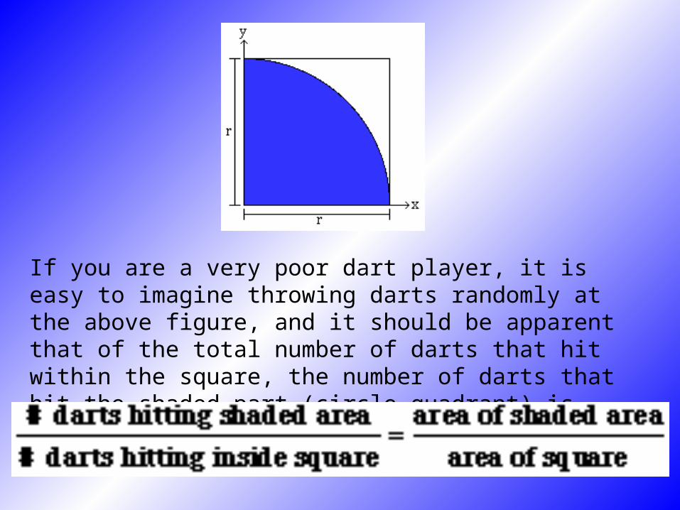
If you are a very poor dart player, it is easy to imagine throwing darts randomly at the above figure, and it should be apparent that of the total number of darts that hit within the square, the number of darts that hit the shaded part (circle quadrant) is proportional to thearea of that part. In other words,

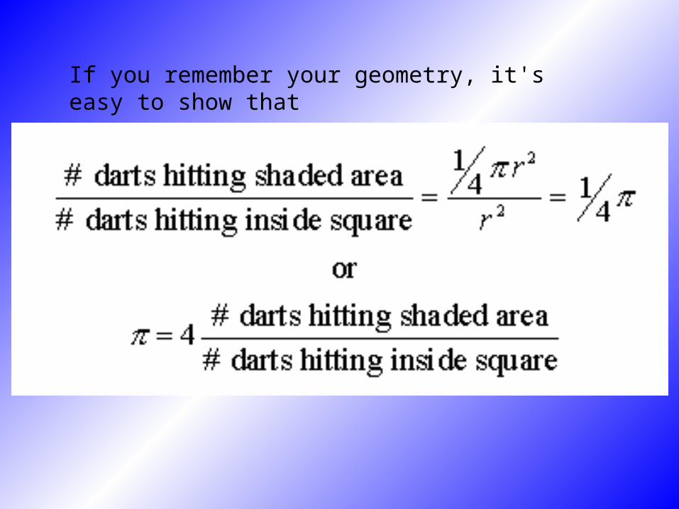
If you remember your geometry, it's easy to show that

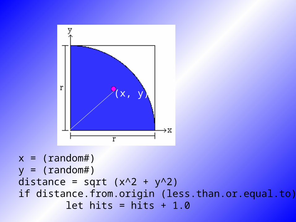
(x, y)

x = (random#) y = (random#) distance = sqrt (x^2 + y^2) if distance.from.origin (less.than.or.equal.to) 1.0 let hits = hits + 1.0

• How did Monte Carlo simulation get its name?

• The name and the systematic development of Monte Carlo methods dates from about 1940’s.

• There are however a number of isolated and undeveloped instances on much earlier occasions.

History of Monte Carlo Method

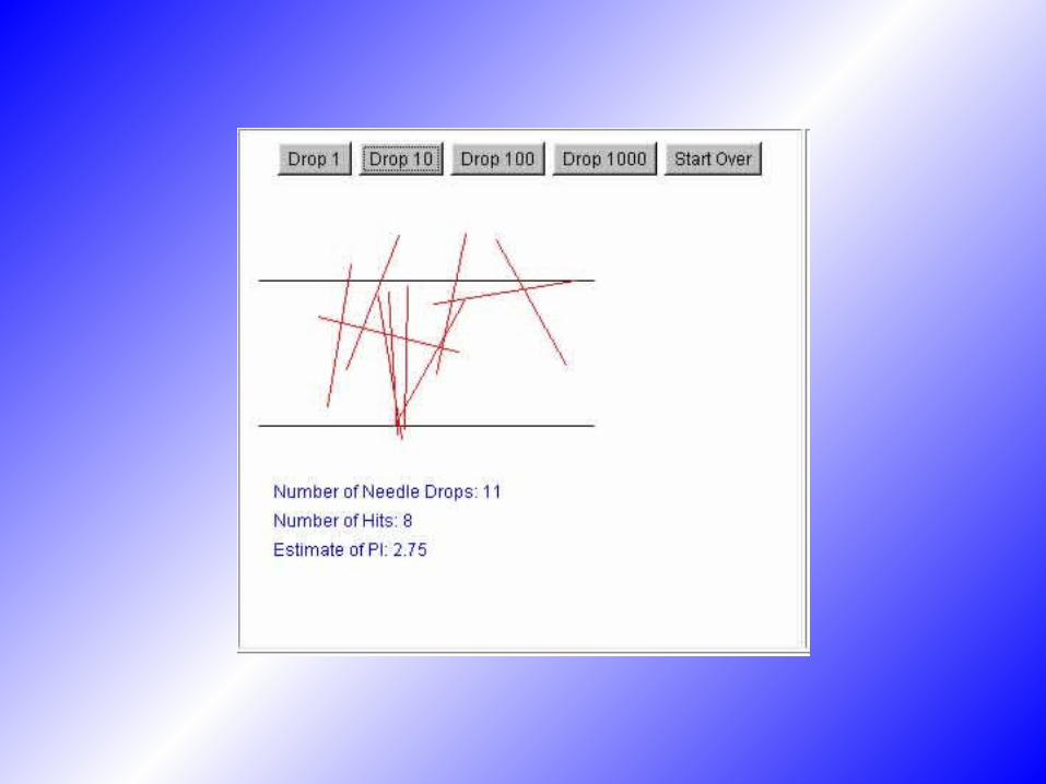
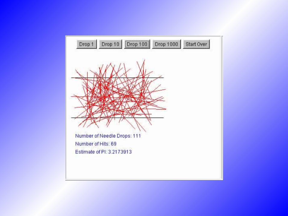
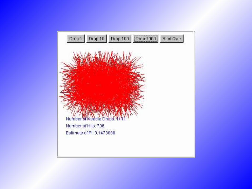
• In the second half of the nineteenth century a number of people performed experiments, in which they threw a needle in a haphazard manner onto a board ruled with parallel straight lines and inferred the value of PI =3.14… from observations of the number of intersections between needle and lines.

• In 1899 Lord Rayleigh showed that a one-dimensional random walk without absorbing barriers could provide an approximate solution to a parabolic differential equation.

History of Monte Carlo method

• In early part of the twentieth century, British statistical schools indulged in a fair amount of unsophisticated Monte Carlo work.

• In 1908 Student (W.S. Gosset) used experimental sampling to help him towards his discovery of the distribution of the correlation coefficient.

• In the same year Student also used sampling to bolster his faith in his so-called t-distribution, which he had derived by a somewhat shaky and incomplete theoretical analysis.

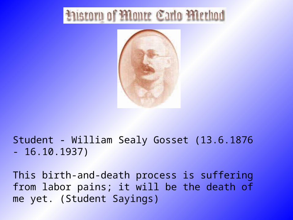
Student - William Sealy Gosset (13.6.1876 - 16.10.1937)

This birth-and-death process is suffering from labor pains; it will be the death of me yet. (Student Sayings)

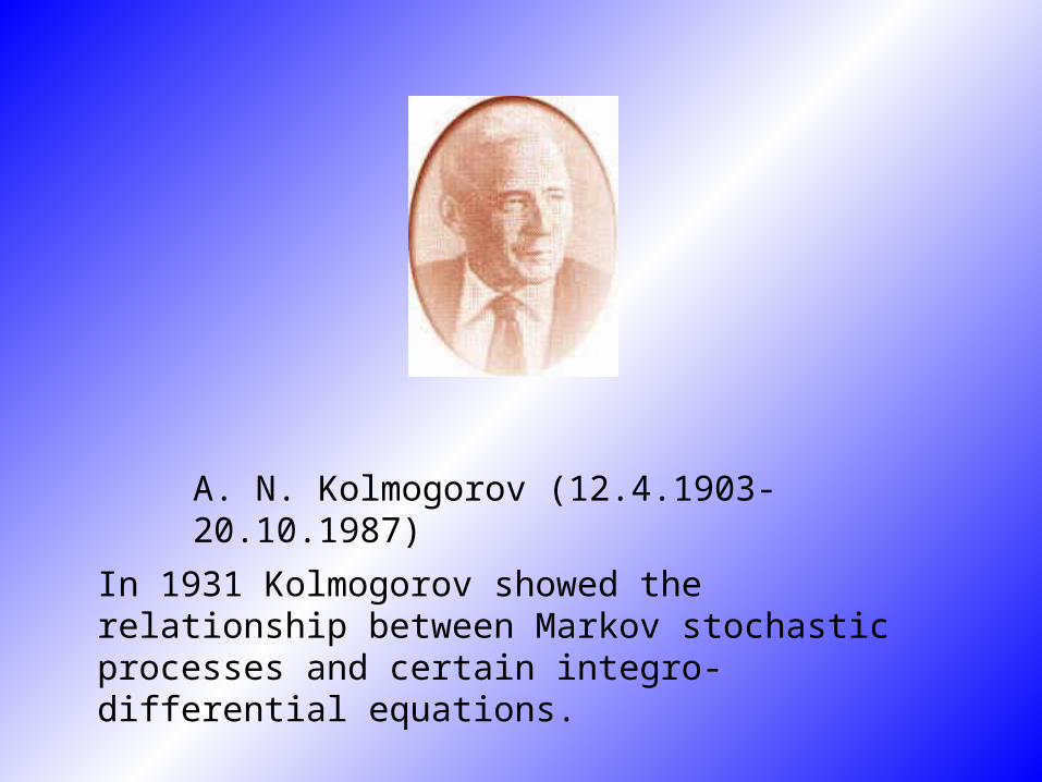
In 1931 Kolmogorov showed the relationship between Markov stochastic processes and certain integro-differential equations.

A. N. Kolmogorov (12.4.1903-20.10.1987)

History (cont.)

• The real use of Monte Carlo methods as a research tool stems from work on the atomic bomb during the second world war.

• This work involved a direct simulation of the probabilistic problems concerned with random neutron diffusion in fissile material; but even at an early stage of these investigations, von Neumann and Ulam refined this particular "Russian roulette" and "splitting" methods. However, the systematic development of these ideas had to await the work of Harris and Herman Kahn in 1948.

• About 1948 Fermi, Metropolis, and Ulam obtained Monte Carlo estimates for the eigenvalues of Schrodinger equation.

John von Neumann (28.12.1903-8.2.1957)

History (cont.)• In about 1970, the newly developing theory of computational

complexity began to provide a more precise and persuasive rationale for employing the Mont Carlo method.

• Karp (1985) shows this property for estimating reliability in a planar multiterminal network with randomly failing edges.

• Dyer (1989) establish it for estimating the volume of a convex body in M-dimensional Euclidean space.

• Broder (1986) and Jerrum and Sinclair (1988) establish the property for estimating the permanent of a matrix or, equivalently, the number of perfect matchings in a bipartite graph.

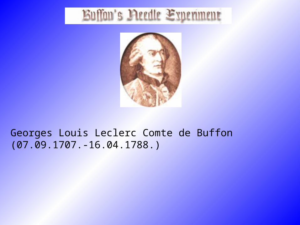
Georges Louis Leclerc Comte de Buffon (07.09.1707.-16.04.1788.)

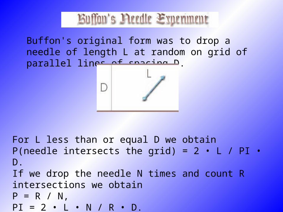
Buffon's original form was to drop a needle of length L at random on grid of parallel lines of spacing D.

For L less than or equal D we obtain P(needle intersects the grid) = 2 • L / PI • D. If we drop the needle N times and count R intersections we obtain P = R / N, PI = 2 • L • N / R • D.

http://www.geocities.com/CollegePark/Quad/2435/history.html

http://www-groups.dcs.st-and.ac.uk/~history/Mathematicians/Kolmogorov.html

http://www-groups.dcs.st-and.ac.uk/~history/Mathematicians/Von_Neumann.html

http://wwitch.unl.edu/zeng/joy/mclab/mcintro.html

http://www.decisioneering.com/monte-carlo-simulation.html

http://www.mste.uiuc.edu/reese/buffon/bufjava.html

Monte Carlo Methods:Application to PDE’s

Chris RambicureGuojin Chen

Christopher Cprek

What I’ll Be Covering

• How Monte Carlo Methods are applied to PDEs.

• An example of a simple integral.• The importance of random numbers.• Tour du Wino: A more advanced example.

Approximating PDEs with Monte Carlo Methods…• The basic concept is that games

of chance can be played to approximate solutions to real world problems.

• Monte Carlo methods solve non-probabilistic problems using probabilistic methods.

A Simple Integral

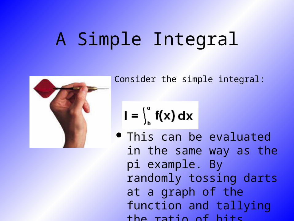
• Consider the simple integral:

This can be evaluated in the same way as the pi example. By randomly tossing darts at a graph of the function and tallying the ratio of hits inside and outside the function.

A Simple Integral (continued…)

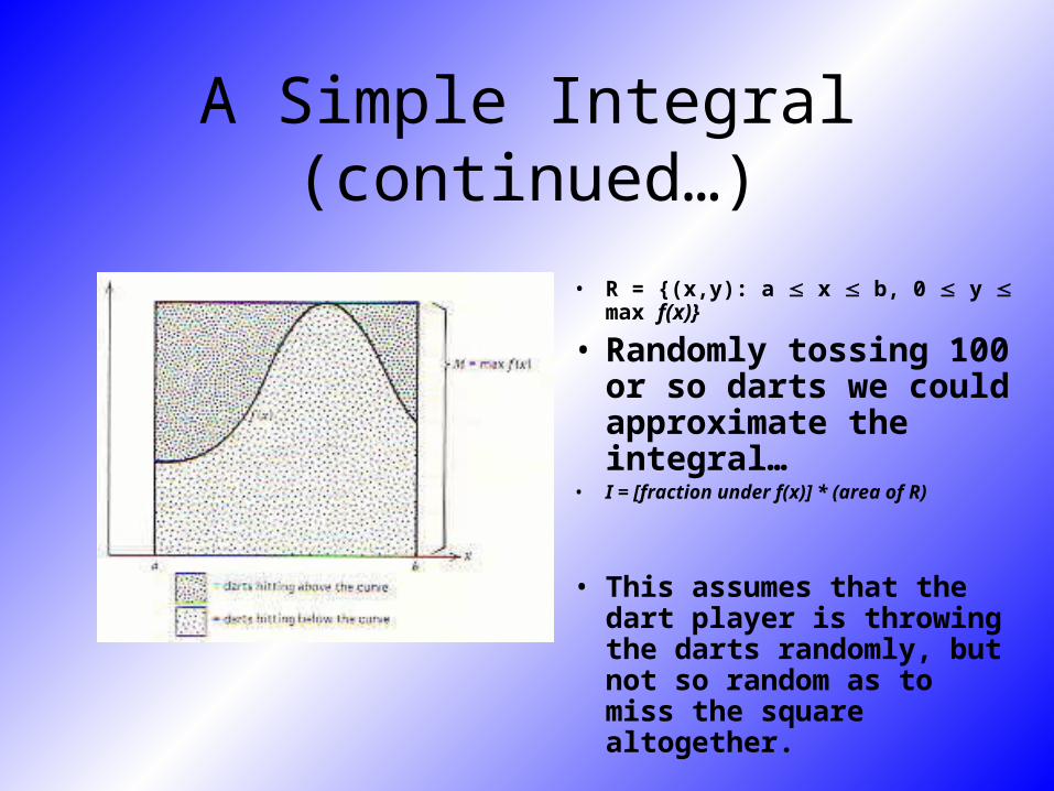
• R = {(x,y): a x b, 0 y max f(x)}

• Randomly tossing 100 or so darts we could approximate the integral…

• I = [fraction under f(x)] * (area of R)

• This assumes that the dart player is throwing the darts randomly, but not so random as to miss the square altogether.

A Simple Integral (continued…)

• Generally, the more iterations of the game the better the approximation will be. 1000 or more darts should yield a more accurate approximation of the integral than 100 or fewer.

• The results can quickly become skewed and completely irrelevant if the games random numbers are not sufficiently random.

The Importance of Randomness

• Say for each iteration of the game the “random” trial number in the interval was exactly the same. This is entirely non-random. Depending on whether or not the trial number was inside or outside of the curve the approximation of integral I would be either 0 or .

• This is the worst approximation possible.

The Importance of Randomness(continued…)

• Also, a repeating sequence will skew the approximation.

• Consider an interval between 1 and 100, where the trials create a random trial sequence24, 19, 74, 38, 45, 38, 45, 38, 45, 38, 45,…

• At worst, 38 and 45 are both above or below the function line and skew the approximation.

• At best, 38 and 45 don’t fall together and you’re just wasting your time.

Random Trials (continued…)

• Very advanced Monte Carlo Method computations could run for months before arriving at an approximation.

• If the method is not sufficiently random, it will certainly get a bad approximation and waste lots of $$$.

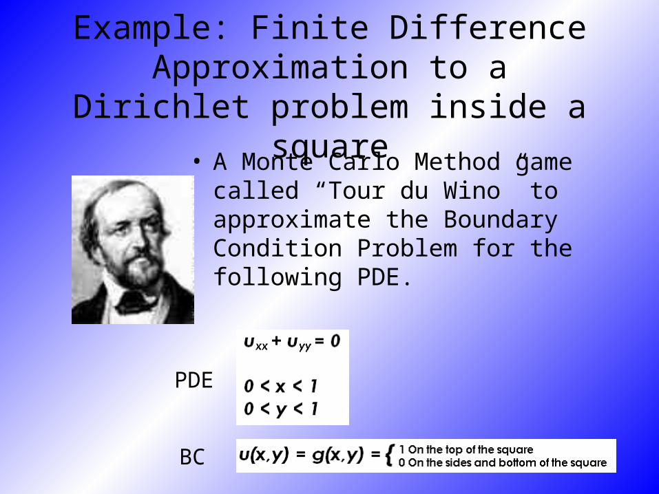
Example: Finite Difference Approximation to a Dirichlet problem

inside a square• A Monte Carlo Method game called

“Tour du Wino” to approximate the Boundary Condition Problem for the following PDE.

PDE

BC

Dirichlet Problem (continued…)

• The Solution to this problem, using the finite difference method to compute it is:

u(i,j) = ¼(u(i-1, j) + u(i+1, j) + u(i,j-1) + u(i,j+1) )u(i,j) = g(i, j) : g(i, j) the solution at boundary

(i,j).

Just remember this for later….

Tour du Wino

• To play we must have a grid with boundaries.

• A drunk wino starts the game at an arbitrary point on the grid A.

• He wanders randomly in one of four directions.

• He begins the process again until he hits a grid boundary.

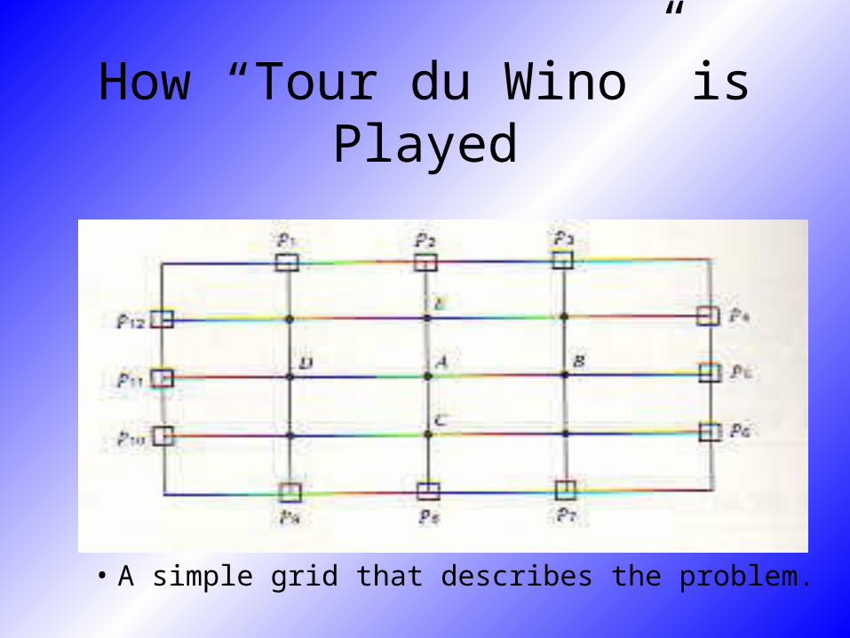
How “Tour du Wino” is Played

• A simple grid that describes the problem.

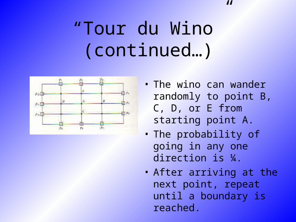
“Tour du Wino” (continued…)

• The wino can wander randomly to point B, C, D, or E from starting point A.

• The probability of going in any one direction is ¼.

• After arriving at the next point, repeat until a boundary is reached.

“Tour du Wino” (continued…)

• The wino will receive a reward g(i) at each boundary p(i). (a number, not

more booze…)• The goal of the game is

to compute the average reward for the total number of walks

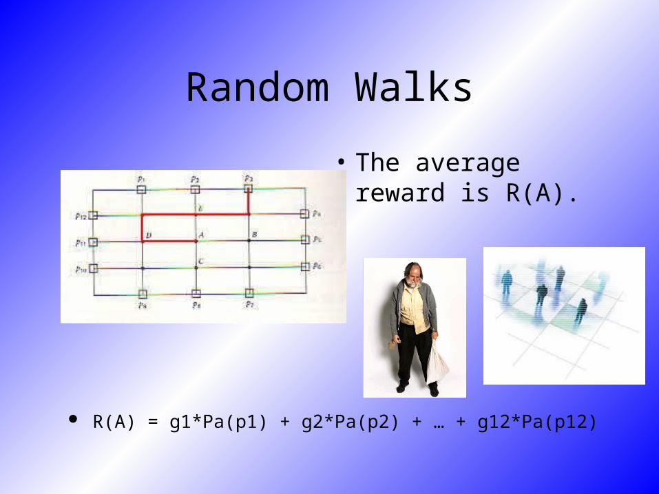
Random Walks

• The average reward is R(A).

R(A) = g1*Pa(p1) + g2*Pa(p2) + … + g12*Pa(p12)

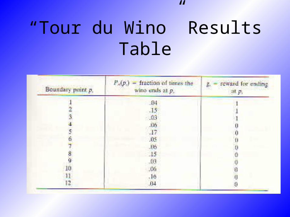
“Tour du Wino” Results Table

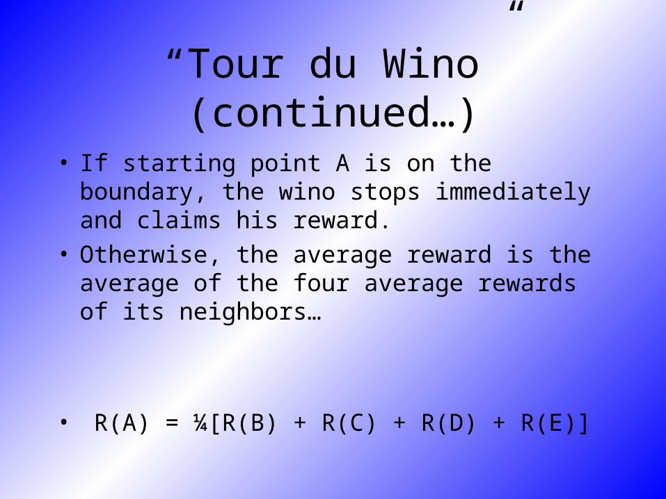
“Tour du Wino” (continued…)

• If starting point A is on the boundary, the wino stops immediately and claims his reward.

• Otherwise, the average reward is the average of the four average rewards of its neighbors…

• R(A) = ¼[R(B) + R(C) + R(D) + R(E)]

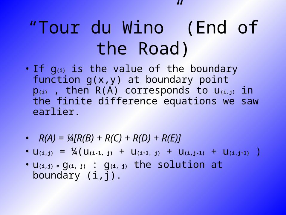
“Tour du Wino” (End of the Road)

• If g(i) is the value of the boundary function g(x,y) at boundary point p(i) , then R(A) corresponds to u(i,j) in the finite difference equations we saw earlier.

• R(A) = ¼[R(B) + R(C) + R(D) + R(E)]• u(i,j) = ¼(u(i-1, j) + u(i+1, j) + u(i,j-1) + u(i,j+1) )• u(i,j) = g(i, j) : g(i, j) the solution at boundary (i,j).

Wrap-Up

• Monte Carlo Methods can be used to approximate solutions to many types of non-probabilistic problems.

• This can be done by creating “random games” that describe the problem and running trials with these games.

• Monte Carlo methods can be very useful to approximate extremely difficult PDEs and many other types of problems.

More References

• http://www.ecs.fullerton.edu/~mathews/fofz/dirichlet/dirichle.html

• http://mathworld.wolfram.com/DirichletProblem.html

• http://wwitch.unl.edu/zeng/joy/mclab/mcintro.html

• Farlow, Stanley Partial Differential Equations for Scientists and EngineersDover Publications, New York 1982

A Few Monte Carlo Applications

Chris RambicureGuojin Chen

Christopher Cprek

What I’ll Be Covering

Markov ChainsQuantum Monte Carlo MethodsWrapping it All Up

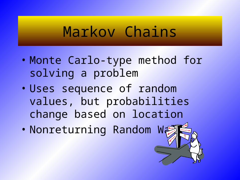
Markov Chains

• Monte Carlo-type method for solving a problem

• Uses sequence of random values, but probabilities change based on location

• Nonreturning Random Walk

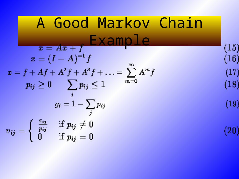
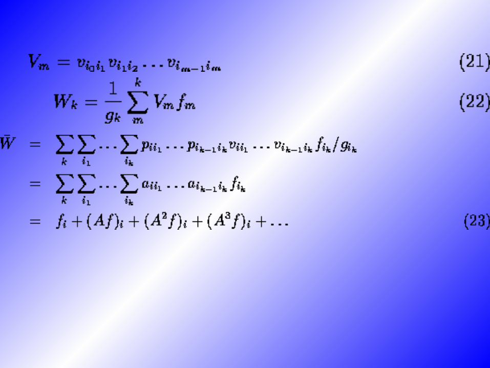
A Good Markov Chain Example

Moving on…..

• The only good Monte Carlo is a dead Monte Carlo.

-Trotter & Tukey

Quantum Monte Carlo

• Uses Monte Carlo method to determine structure and properties of matter

• Obviously poses Difficult Problems• But gives Consistent and Accurate Results

A Few Problems Using QMC

• Surface Chemistry• Metal-Insulator

Transitions• Point Defects in Semi-

Conductors• Excited States

• Simple Chemical Reactions

• Melting of Silicon• Determining Smallest

Stable Fullerene

Why Use QMC?

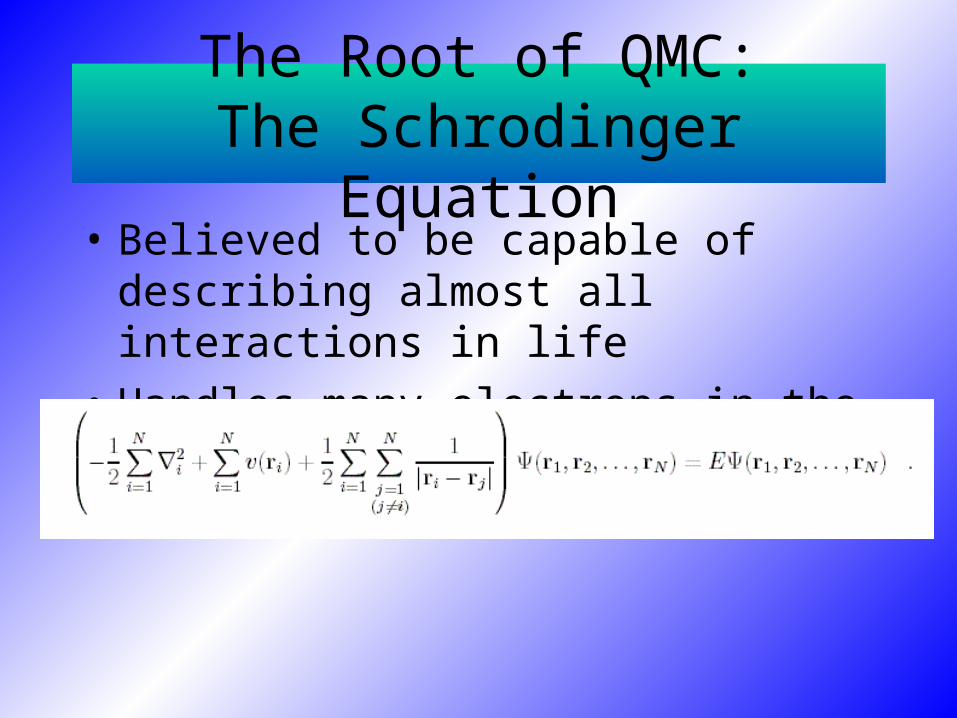
The Root of QMC:The Schrodinger Equation

• Believed to be capable of describing almost all interactions in life

• Handles many electrons in the equation

Variational QMC (VMC)

• One Type of QMC• Kind of Needs Computers• Generate sets of Random positions as

Result of Comparing Electron Positions to the many-electron wavefunction

Difficulties With VMC

• The many-electron wavefunction is unknown• Has to be approximated• Use a small model system with no more than

a few thousand electrons• May seem hopeless to have to actually guess

the wavefunction• But is surprisingly accurate when it works

The Limitation of VMC

• Nothing can really be done if the trial wavefunction isn’t accurate enough

• Therefore, there are other methods• Example: Diffusion QMC

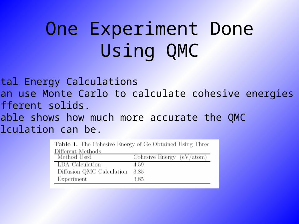
One Experiment Done Using QMC

Total Energy Calculations-Can use Monte Carlo to calculate cohesive energies ofdifferent solids.-Table shows how much more accurate the QMCcalculation can be.

The End

• Monte Carlo methods can be extremely useful for solving problems that aren’t approachable by normal means

• Monte Carlo methods cover a variety of different fields and applications.

My Sources• Foulkes, et al. “Quantum Monte Carlo Simulations of Real Solids.”

Online. http://www.tcm.phy.cam.ac.uk/~mdt26/downloads/hpc98.pdf.• Carter, Everett. “Markov Chains.” Random Walks, Markov Chains,

and the Monte Carlo Method. Taygeta Scientific Inc. Online. http://www.taygeta.com/rwalks/node7.html.

• Needs, et al. “Quantum Monte Carlo: Theory of Condensed Matter Group.” Online. http://www.tcm.phy.cam.ac.uk/~mdt26/cqmc.html.