monocular rivalry exhibits three hallmarks of binocular rivalry: evidence for common processes

Vision Research 49 (2009) 671–681

Contents lists available at ScienceDirect

Vision Research

journal homepage: www.elsevier .com/locate /v isres

Monocular rivalry exhibits three hallmarks of binocular rivalry: Evidencefor common processes

Robert P. O’Shea a,*, Amanda Parker b, David La Rooy a, David Alais b

a Department of Psychology, University of Otago, P.O. Box 56, Dunedin, New Zealandb School of Psychology, The University of Sydney, Australia

a r t i c l e i n f o

Article history:Received 20 April 2008Received in revised form 29 December 2008

Keywords:Monocular rivalryBinocular rivalryColourPerceptual ambiguityVisionVisual suppressionDepth of suppression

0042-6989/$ - see front matter � 2009 Elsevier Ltd. Adoi:10.1016/j.visres.2009.01.020

* Corresponding author.E-mail address: [email protected] (R.P. O’Shea).

a b s t r a c t

Binocular rivalry occurs when different images are presented one to each eye: the images are visible onlyalternately. Monocular rivalry occurs when different images are presented both to the same eye: the clar-ity of the images fluctuates alternately. Could both sorts of rivalry reflect the operation of a general visualmechanism for dealing with perceptual ambiguity? We report four experiments showing similaritiesbetween the two phenomena. First, we show that monocular rivalry can occur with complex images,as with binocular rivalry, and that the two phenomena are affected similarly by the size (Experiment1) and colour (Experiment 2) of the images. Second, we show that the distribution of dominance periodsduring monocular rivalry has a gamma shape and is stochastic (Experiment 3). Third, we show that dur-ing periods of monocular-rivalry suppression, the threshold to detect a probe (a contrast pulse to the sup-pressed stimulus) is raised compared with during periods of dominance (Experiment 4). The thresholdelevation is much weaker than during binocular rivalry, consistent with monocular rivalry’s weakappearance. We discuss other similarities between monocular and binocular rivalry, and also some dif-ferences, concluding that part of the processing underlying both phenomena is a general visual mecha-nism for dealing with perceptual ambiguity.

� 2009 Elsevier Ltd. All rights reserved.

1. Introduction

We experience the visual world in astounding richness and de-tail, yet our knowledge of how our conscious percepts arise is stillquite poor (cf. Chalmers, 1995). One way to learn more about theseprocesses is to study phenomena in which visual consciousnesschanges without any change in the stimuli being viewed (Crick &Koch, 1995). Such phenomena are known as perceptually multista-ble and include binocular rivalry (Porta, 1593, cited in Wade, 1996),reversals of the Necker cube (Necker, 1832), of the Rubin face-vasefigure (Rubin, 1915), and of the kinetic depth effect (Wallach &O’Connell, 1953), and motion-induced blindness (Bonneh, Cooper-man, & Sagi, 2001). Binocular rivalry is a particularly fascinatingexample, in which visual consciousness fluctuates randomly be-tween two different images presented one to each eye. It has beenstudied extensively (for reviews see Alais & Blake, 2005; Blake &O’Shea, 2009) and has gone some way to shedding light on how vi-sual awareness arises: conscious visual experience in binocular riv-alry is thought to arise from activation, and suppression, of neuronsat a succession of stages in the visual system via feed-forward andfeedback connections (e.g., Blake & Logothetis, 2002).

ll rights reserved.

Our interest in this paper is in the relationship between binoc-ular rivalry and another phenomenon of perceptual multistability,monocular rivalry. Monocular rivalry was discovered by Breese(1899) in the course of his foundational observations and experi-ments on binocular rivalry. He found that binocular rivalry-likebehaviour also occurred when a red and a green grating were opti-cally superimposed by a prism and presented to a single eye. Bre-ese called it monocular rivalry to distinguish it from binocularrivalry. He reported that monocular rivalry alternations tended tooccur at a slower rate than binocular rivalry alternations and thatthe perceptual alternations were less vivid: ‘‘Neither [stimulus]disappeared completely: but at times the red would appear verydistinctly while the green would fade; then the red would fadeand the green appear distinctly” (p. 43).

One of the unresolved questions in the literature on perceptualmultistability is whether common neural mechanisms underliebinocular and monocular rivalry. Rubin (2003), Leopold and Logo-thetis (1999), and Maier, Logothetis, and Leopold (2005) have pro-posed that all examples of perceptual multistability representoperations of a single, high-level mechanism. If so, this would tietogether diverse multistability phenomena including perceptionof ambiguous auditory stimuli (e.g., Einhäuser, Stout, Koch, & Car-ter, 2008), perception of traditional visual ambiguous figures suchas the Necker cube (e.g., Meng & Tong, 2004), perception of illusory

mailto:[email protected]

http://www.sciencedirect.com/science/journal/00426989

http://www.elsevier.com/locate/visres

672 R.P. O’Shea et al. / Vision Research 49 (2009) 671–681

organisation such as Marroquin patterns (Wilson, Krupa, & Wilkin-son, 2000), monocular rivalry, and binocular rivalry.

There are at least three general similarities between monocularrivalry and binocular rivalry that suggest commonality. The basicphenomenology is similar in that both involve periods of alternat-ing dominance. Both forms of rivalry become more vigorous asstimuli are made more different in colour (e.g., Wade, 1975), orin orientation and spatial frequency (e.g., Atkinson, Fiorentini,Campbell, & Maffei, 1973; Campbell, Gilinsky, Howell, Riggs, &Atkinson, 1973; O’Shea, 1998). The two forms of rivalry can influ-ence each other, tending to synchronise their alternations in adja-cent regions of the visual field (Andrews & Purves, 1997; Pearson &Clifford, 2005).

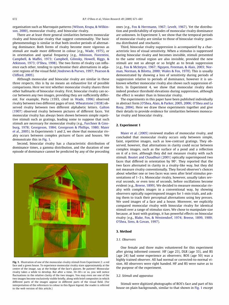
Although monocular and binocular rivalry are similar in thesethree respects, this is by no means an exhaustive list of possiblecomparisons. Here we test whether monocular rivalry shares threeother hallmarks of binocular rivalry. First, binocular rivalry can oc-cur between any two images, providing they are sufficiently differ-ent. For example, Porta (1593, cited in Wade, 1996) observedrivalry between two different pages of text. Wheatstone (1838) ob-served rivalry between two different alphabetic letters. Galton(1907) observed rivalry between pictures of different faces. Yetmonocular rivalry has always been shown between simple repeti-tive stimuli such as gratings, leading some to suppose that suchstimuli are necessary for monocular rivalry (e.g., Furchner & Gins-burg, 1978; Georgeson, 1984; Georgeson & Phillips, 1980; Maieret al., 2005). In Experiments 1 and 2, we show that monocular riv-alry occurs between complex pictures of faces and houses. Wedemonstrate this in Fig. 1.

Second, binocular rivalry has a characteristic distribution ofdominance times, a gamma distribution, and the duration of oneepisode of dominance cannot be predicted by any of the preceding

Fig. 1. Illustration of one of the monocular-rivalry stimuli from Experiment 2: a redface and a green house. To experience monocular rivalry stare approximately at thecentre of the image, say at the bridge of the face’s glasses. Be patient! Monocularrivalry takes a while to develop. But after a time, 10–30 s or so, you will noticefluctuations in the relative clarity of the two images. You may even see one of thetwo images become exclusively visible briefly, along with brief composites in whichdifferent parts of the images appear in different parts of the visual field. (Forinterpretation of the references to colour in this figure legend, the reader is referredto the web version of this article.)

ones (e.g., Fox & Herrmann, 1967; Levelt, 1967). Yet the distribu-tion and predictability of episodes of monocular rivalry dominanceare unknown. In Experiment 3, we show that the temporal periodsof monocular rivalry are similar to those of binocular rivalry: gam-ma distributed and stochastic.

Third, binocular rivalry suppression is accompanied by a char-acteristic loss of visual sensitivity. When a stimulus is suppressedduring binocular rivalry and becomes invisible, stimuli presentedto the same retinal region are also invisible, provided the newstimuli are not so abrupt or so bright as to break suppression(e.g., Fox & McIntyre, 1967; Nguyen, Freeman, & Alais, 2003; Nor-man, Norman, & Bilotta, 2000; Wales & Fox, 1970). This is usuallydemonstrated by showing a loss of sensitivity during periods ofsuppression relative to periods of dominance, however it is un-known whether monocular rivalry also shows such suppression ef-fects. In Experiment 4, we show that monocular rivalry doesindeed produce threshold elevations during suppression, althoughthe effect is weaker than in binocular rivalry.

The experiments in this paper have been published individuallyin abstract form (O’Shea, Alais, & Parker, 2005, 2006; O’Shea and LaRooy, 2004). Here we draw these experiments together and givetheir details to provide evidence for similarities between monocu-lar rivalry and binocular rivalry.

2. Experiment 1

Maier et al. (2005) reviewed studies of monocular rivalry, andconcluded that monocular rivalry occurs only between simple,faint, repetitive images, such as low-contrast gratings. They ob-served, however, that alternations in clarity could occur betweencomplex images, such as the surface of a pond and a reflectionon it of a tree, although they did not measure rivalry with suchstimuli. Boutet and Chaudhuri (2001) optically superimposed twofaces that differed in orientation by 90�. They reported that thetwo faces alternated in clarity in a rivalry-like way, but they didnot measure rivalry conventionally. They forced observer’s choicesabout whether one or two faces was seen after brief stimulus pre-sentations of 1–3 s. Monocular rivalry, however, usually takes sev-eral seconds, or even tens of seconds, before oscillations becomeevident (e.g., Breese, 1899). We decided to measure monocular riv-alry with complex images in a conventional way, by showingobservers optically superimposed images for 1-min trials, and ask-ing them to track their perceptual alternations using key presses.We used images of a face and a house. Moreover, we explicitlycompared monocular rivalry with binocular rivalry for identicalstimuli over a range of stimulus sizes. We chose to manipulate sizebecause, at least with gratings, it has powerful effects on binocularrivalry (e.g., Blake, Fox, & Westendorf, 1974; Breese, 1899, 1909;O’Shea, Sims, & Govan, 1997).

3. Method

3.1. Observers

One female and three males volunteered for this experimentafter giving informed consent: HF (age 23), DLR (age 33), and RS(age 24) had some experience as observers; ROS (age 50) was ahighly trained observer. All had normal or corrected-to-normal vi-sion. All observers were right handed. HF and RS were naive as tothe purpose of the experiment.

3.2. Stimuli and apparatus

Stimuli were digitized photographs of ROS’s face and part of hishouse on plain backgrounds, similar to that shown in Fig. 1 except

R.P. O’Shea et al. / Vision Research 49 (2009) 671–681 673

that they were greyscale. Stimuli were 0.77�, 1.54�, 3.08�, 6.16�,and 12.32� of visual angle square. The smaller images were allscaled-down versions of largest image (800 � 800 pixels) and scal-ing was done using NIH Image software. (Scaling from large tosmall minimises spatial frequency distortions that can arise whenscaling from small to large). They were surrounded by two brightvertical bars, each 0.5� wide, as tall as the stimulus, and separatedfrom the edge of the stimulus by 0.5�; these were to help observersalign the stimuli binocularly. Stimuli were displayed on two iden-tical Sony Trinitron, 19-in., colour monitors with a spatial resolu-tion of 1152 � 870 pixels and a frame rate of 75 Hz. Each eye ofthe observer viewed only one monitor from a distance of 1 mthrough a mirror stereoscope. The experiment was controlled bya Power Macintosh 8600 computer running specially written soft-ware (Handley, Bevin, & O’Shea, 2005).

The room was entirely dark, with the monitors as the sole lightsource. Presenting superimposed images of the face and house toboth eyes created monocular rivalry. Presenting the image of theface and house separately to each eye created binocular rivalry.The luminance of the stimuli on each screen was 10 cd/m2, and thatof the vertical bars was 30 cd/m2. Otherwise the screens were dark(0.2 cd/m2). The standard deviation of the luminances in the twoimages was 2.45 cd/m2 for the face and 3.44 cd/m2 for the house.

3.3. Procedure

There were two sessions each containing a block of 10 binocularrivalry trials and a block of 10 monocular-rivalry trials. In eachblock, observers received two presentations of the images at eachof the five image sizes. During binocular rivalry trials, one presen-tation of each stimulus size was of the face to the left eye and thehouse to the right eye, and the other was of the opposite arrange-ment. Order of trials was random within blocks. Order of blockswas counterbalanced over observers and over sessions.

Each trial lasted for 60 s and was followed by an inter-trialinterval of at least 45 s. Observers reported their perception ofeither the face or house by pressing the ‘Z’ or ‘?’ keys, respectively.They pressed a key whenever, and for as long as, a particular stim-ulus exceeded a criterion level of visibility. For binocular rivalry,this criterion was that an image was exclusively visible over atleast 95% of the field. For monocular rivalry, this criterion was thatan image appeared to be at least twice as clear as the other, or wasexclusively visible over at least two-thirds of the field (we call thisa 66% visibility criterion).

The experimental sessions were preceded by sufficient practicetrials to enable each observer to respond consistently to both sortsof rivalry.

0

2

4

6

8

10

12

0.77 1.54 3.08 6.16 12.32Size (deg)

MR

BR

Rat

e (a

lts/m

in)

Fig. 2. Plot of binocular rivalry (BR) and monocular-rivalry (MR) rate (the numberof episodes of dominance of each image per minute) against size of the images. Thevertical bars show ±1 standard error of the mean.

4. Results and discussion

All observers found it easy to press keys to signal their percep-tion of the two images in both monocular and binocular rivalry.They also commented on some of their unusual perceptions. Dur-ing binocular rivalry, they sometimes described composites, inwhich one image would replace the other over a few moments.For example, one might briefly see the left half of the face onthe left side of the screen and the right half of the house onthe right side of the screen before the face would then wipeout the remaining image of the house. More amusingly, onemight briefly see the face with one eye replaced by the house’swindow. Such composites are a common property of binocularrivalry, and have been studied by Wilson, Blake, and Lee (2001).Observers reported similar composites during monocular rivalry.

We quantified rivalry in three ways. First, we counted the num-ber of times each key was pressed to obtain a rate measure of riv-

alry. Second, we counted the cumulative time each key waspressed to obtain a measure of dominance time. Third, we averagedthe time of each individual key press to obtain a measure we callperiod.

We analysed these data with three-factor, within-subjects ANO-VAs (the factors were type of rivalry, size, and image reported).There was a significant effect of size on rate, F(4,12) = 12.29,p < .001, such that rate increased with size of the images (seeFig. 2). All observers showed this pattern of results. An increasingalternation rate with image size is opposite to the usual finding withsimple stimuli such as gratings (e.g., Breese, 1899; O’Shea et al.,1997). Critically, there was no difference between monocular andbinocular rivalry in the shape of the function relating size to rate.

There was also one significant effect for dominance time: theface was seen for longer than the house, F(1,3) = 10.64, p < .05.The mean dominance time for the face was 12.44 s (SD = 9.95 s)and that for the house was 6.90 s (SD = 5.47 s). This could havearisen from a general preference for faces over other stimuli in riv-alry (e.g., Beloff & Beloff, 1959; Engel, 1956) or from some prefer-ence for the spatial frequencies of the face image over the houseimage (cf. Lumer, Friston, & Rees, 1998; Tong, Nakayama, Vaughan,& Kanwisher, 1998). But it is not important for our purposes, be-cause there were no other significant effects or interactions for thismeasure, showing that this advantage for the face was consistentover size and over type of rivalry.

There were no significant effects for period. These were similarover stimuli, over sizes, and over the two sorts of rivalry.

The increase in the rate of alternations with size for both sortsof rivalries is consistent with the idea that rivalry between com-plex stimuli is mediated by interactions among neurons in high-er-level visual areas such as the inferotemporal cortex (Alais &Melcher, 2007; Sheinberg & Logothetis, 1997). Not only are suchneurons responsive to coherent visual objects, such as the houseand face stimuli used here, their receptive fields are far larger thanthose at earlier levels of the visual system (Gross, Bender, & Rocha-Miranda, 1969; Yoshor, Bosking, Ghose, & Maunsell, 2007) andwould therefore be preferentially activated by the larger rivalstimuli.

One possible alternative explanation is that image size is corre-lated with spatial-frequency content. This might seem plausiblebecause with grating stimuli, monocular rivalry is usually stron-gest at low spatial frequencies (Kitterle & Thomas, 1980; Mapper-son & Lovegrove, 1984; O’Shea, 1998). But grating stimuli containonly a single spatial frequency, whereas our images are complexwith a very broad spatial frequency spectrum that follows a fractal(1/f) amplitude profile. Such images are scale invariant (e.g., Field,

MonocularBinocular

Rivalry

ColouredAchromatic

0

2

4

6

8

10

12

14

Rat

e (a

lts/m

in)

Fig. 3. Plot of binocular rivalry and monocular-rivalry rate (the number of episodesof dominance of each image per minute) for achromatic and for coloured images.The vertical bars show ±1 standard error of the mean.


1994; Ruderman & Bialek, 1994) Complex images therefore showthe same complex mix of spatial frequencies at all sizes of images.

Of more central importance for our purposes is that both mon-ocular rivalry and binocular rivalry, which is robust over a verylarge range of spatial frequencies (O’Shea et al., 1997), exhibitedthe same trend of increasing alternation rate with increasing imagesize. Given this, the similar trends shown in Fig. 2 may be indica-tive of common mechanisms in monocular and binocular rivalry.We further test this idea in the next experiment by assessing theeffects on the two sorts of rivalries of adding colour differencesto the two rivalling images.

5. Experiment 2

Monocular rivalry does not require coloured stimuli (e.g.,Experiment 1), but its alternation rate is faster when stimuli havecomplementary colours (Campbell & Howell, 1972; Rauschecker,Campbell, & Atkinson, 1973; Wade, 1975). Similarly, binocular riv-alry does not require coloured stimuli, but its alternation rate isalso faster when the rival stimuli have complementary colours(Hollins & Leung, 1978; Thomas, 1978; Wade, 1975). The onlystudies we are aware of in which the effects of colour on monocu-lar and binocular rivalry were compared in the same experimentwith the same observers’ viewing grating stimuli came to differentconclusions. Kitterle and Thomas (1980) found that colour affectedmonocular but not binocular rivalry whereas Knapen, Kanai, Bras-camp, van Boxtel, and van Ee (2007) found that colour affectedmonocular and binocular rivalry similarly. In Experiment 2, we alsoexamine the role of colour on binocular and monocular rivalry butextend it to include complex broadband images.

6. Method

The Method of Experiment 2 was very similar to that of Exper-iment 1. The differences were that a second set of stimuli, that usedby Tong et al. (1998) was added, and one of the male observers (RS)from Experiment 1 did not participate. All stimuli were 6.16�square. Tong et al.’s stimuli were similar to those of Experiment1, except that they comprised a different male face (younger,clean-shaven, and without glasses) and a different house (older,of a Georgian style, and showing more elaborate architectural de-tails). Pixel luminances in Tong et al.’s face and house had standarddeviations of 3.22 cd/m2 and 4.98 cd/m2, respectively. There were12 binocular rivalry and 12 monocular-rivalry trials in whichobservers again tracked their rivalry alternations. In four repeti-tions of each pair of stimuli the images were achromatic, in fourthe face was red (CIE x = .315, y = .321) and the house green (CIEx = .270, y = .347), and in four the face was green and the housered. Mean luminances of all stimuli (colour and greyscale) werethe same as that in Experiment 1. See Fig. 1 for an illustration ofone of the monocular-rivalry stimuli.


Again observers had no trouble recording perceptual alterna-tions in monocular and binocular rivalry, and again they reportedepisodes of composites for both types of rivalry.

We analysed the same three measures of rivalry with four-fac-tor, within-subjects ANOVAs (the factors were type of rivalry, col-our, stimulus set, and image reported). The only significant effectwas colour on rivalry rate, F(1,2) = 19.87, p < .05, such that thealternation rate was greater with coloured images than with achro-matic images (see Fig. 3). All observers showed this pattern of re-sults. The difference between the rates for monocular andbinocular rivalry was not significant, F(1,2) = 5.19, p > .15.

Fig. 3 shows that adding colour differences to two complexrivalling images increases the rate of both monocular and binocu-lar rivalry (the interaction between type of rivalry and colour wasnot significant, F(1,2) = 0.03) without consistently affecting theother measures of rivalry. This is different from the result of Kit-terle and Thomas (1980) who found that colour enhanced monoc-ular rivalry between gratings, but did not enhance binocularrivalry. Although it is possible that this indicates a difference be-tween simple and complex stimuli, we suspect that there is someother explanation, especially because others did find that colourdifferences enhanced binocular-rivalry rates with gratings (Hollins& Leung, 1978; Thomas, 1978; Wade, 1975). For example, Kitterleand Thomas’s binocular-rivalry rates for achromatic stimuli wereabout four times greater than their monocular-rivalry rates. Possi-bly, then, a ceiling effect limited the scope for binocular rivalry tobe enhanced by coloured stimuli.

In any case, we are confident that with complex stimuli, addingdifferent colours to different complex images does enhance bothbinocular and monocular rivalry. This is consistent with some gen-eral rivalry mechanism that assesses the degree of difference be-tween representations of two images and instigates rivalryaccordingly. Adding different colour to different images adds an-other dimension along which the stimuli differ, which would beexpected to lead to more vigorous rivalry. In a related vein, addingcolour to rival images also tends to reduce piecemeal rivalry, be-cause it adds a unifying attribute to each image and tends to leadto more coherent alternations.

By concentrating on overall rivalry alternation rates in the firsttwo experiments, we have ignored the finer-grained temporaldynamics of rivalry. In Experiment 3, we will conduct a comparisonof monocular and binocular rivalry on a finer temporal scale.

8. Experiment 3

The temporal dynamics of binocular rivalry have been wellstudied. For example, Levelt (1968) showed that the distributionof dominance times approximates a gamma function. Moreover,Levelt demonstrated that the duration of one episode of dominanceof one image cannot be predicted from the duration of any of theprevious episodes, meaning that each dominance episode is a sta-tistically independent sample from an underlying population dis-tribution of dominance times. We set out to determine whethermonocular rivalry also conforms to these principles, comparing itwith binocular rivalry dynamics measured on identical binocular-rivalry stimuli. In this we were following the example of van Box-tel, van Ee, and Erkelens (2007) who used similar comparisons to


argue that binocular rivalry and dichoptic masking share similarprocessing.

Essentially all of the studies of the temporal properties of binoc-ular rivalry have used simple repetitive stimuli such as gratings.For comparability with these studies, we use grating stimuli forboth monocular and binocular rivalry.

9. Method

9.1. Observers

Three of the authors acted as observers, along with four inexpe-rienced observers who were unaware of the aims of the experi-ment. All observers had normal vision.

9.2. Apparatus

The computer controlling this experiment was a Macintosh G5,running Matlab 7.0.4 scripts that used the Psychophysics Toolbox(Brainard, 1997; Pelli, 1997). Stimuli were displayed on a 14-in.DiamondPro monitor showing 800 � 600 pixels at a 90 Hz verticalrefresh rate (75 Hz for observers DL, ROS, SM, SS). Stimuli wereshown one on each side of the screen and viewed via a mirror ste-reoscope at a viewing distance of 57 cm.

9.3. Stimuli

Stimuli were two orthogonal square-wave gratings, one red andthe other green, oriented ±45� to vertical. The gratings had a spatialfrequency of 2.2 cycles/deg with a Michelson contrast of 8% andwere placed in a circular aperture subtending 4.6�. Gratings hada mean luminance of 31.30 cd/m2; the background had the sameluminance. The gratings were superimposed and visible to botheyes for monocular rivalry conditions; the gratings were presentedone to each eye for binocular rivalry conditions.

9.4. Procedure

For both binocular and monocular rivalry, the observer’s taskwas similar to that in Experiments 1 and 2: to track episodes ofperceptual dominance of one and the other stimuli by pressingkeys on the computer keyboard. There were two trials lasting upto 5 min for each viewing condition. Viewing condition was alter-nated for each observer over trials; each observer started with adifferent condition.


We analysed the records of rivalry in two ways. First, we plotteddistributions of dominance periods to which we fitted a gammadistribution. However, we also tried fitting a gamma distributionto the reciprocal of dominance duration (alternation rate), follow-ing Brascamp, van Ee, Pestman, and van den Berg’s (2005) recom-mendation that the gamma distribution provides a better fit toalternation rates than to the more commonly used dominancedurations. When we compared fits to both types of data usingthe Kolmogorov–Smirnov goodness-of-fit test (the cumulativefunctions for this test were calculated without binning the data),we found they fitted equally well. Using a critical p-value of 0.10(as in Brascamp et al., 2005), we found that three out of 14 distri-butions of duration data were significantly different from the best-fitting gamma distribution. For the same analysis based on the ratedata, the outcome was the same: three out of 14 distributions dif-fered significantly from the best fit. Although Brascamp et al. didfind rate-based fits to be better (based on nearly 200 distributions),

there was no difference in our small sample. For this reason, and tomake it easier to relate our findings to the previous literature(where duration-based fits have been the standard), we show dis-tributions of dominance periods together with best-fitting gammadistributions of the following form:

f ðtjk; k; aÞ ¼ a1

kkCðkÞtk�1e

tk

where k is the ‘‘scale” parameter, k is the ‘‘shape” parameter, and ascales the height (amplitude) of the distribution.

Fig. 4 shows the distributions of dominance periods separatelyfor monocular and binocular rivalry for four observers (the resultsof the other three observers were similar). We show the fittedgamma functions with their parameters. The parameters of all fitsare remarkably similar, showing that monocular and binocular riv-alry exhibit globally similar alternation dynamics.

Second, we computed autocorrelations between the recordeddominance sequence and the same sequence offset by various timelags in order to test the sequential independence of rivalry domi-nance times. Fig. 5 shows the autocorrelation analyses from thesame four observers for binocular and monocular rivalry. The cor-relation is arbitrarily 1.0 when there is no lag, and the error barsshow 95% confidence intervals (computed from 1000 iterationsof a bootstrapping procedure). Similar to binocular rivalry (Levelt,1968) there is no systematic tendency in monocular rivalry for a gi-ven dominance duration to be related to the previous dominanceduration, or to dominance durations several phases earlier. Overthe seven observers tested at 12 phase lags for monocular and bin-ocular rivalry (a total of 168 points), there are only nine significantdeviations from zero – about what would be expected from type Ierrors with our 95% confidence intervals (9/168 = 0.053).

In summary, the results of this experiment show that monocu-lar rivalry possesses the characteristic temporal dynamics of binoc-ular rivalry. The remaining hallmark of binocular rivalry is thatthere is an objectively measurable suppression of vision of one orthe other images. In Experiment 4, we will search for the same sup-pression in monocular rivalry.

11. Experiment 4

One technique commonly used to study binocular rivalry hasbeen to measure the depth of suppression. This is done by measur-ing the detection threshold for a probe stimulus presented to aneye during suppression, and comparing it against the thresholdfor the same probe measured during dominance (Blake & Camisa,1979; Blake & Fox, 1974; Fox & Check, 1972; Wales & Fox, 1970).Generally, for simple stimuli such as gratings and contours, probesensitivity is reduced during suppression to about 60% of the levelmeasured during dominance (Fox & McIntyre, 1967; Nguyen et al.,2003; Norman et al., 1999; Wales & Fox, 1970).

Surprisingly, the probe technique has never been used to assessthe depth of monocular-rivalry suppression. We set out to do so. Ofcourse, it is not possible to use monocular probes (as done in bin-ocular rivalry probe experiments) for monocular rivalry becausethe rivalling stimuli are both present in the same eye. Instead,our approach was to use a contrast increment of one of the monoc-ular-rivalry stimuli as a probe. Again, for comparability with previ-ous research, we used orthogonal gratings as rivalry stimuli.Gratings were red or green, oriented ±45� to vertical. We brieflyand smoothly pulsed the contrast of the red grating according toa temporal Gaussian profile, varying the amplitude of the pulseto find the threshold. These thresholds were measured duringdominance and suppression to quantify suppression depth formonocular rivalry. As a comparison, we also measured suppressiondepth for the same stimuli under binocular rivalry conditions.

Fig. 4. Distributions of dominance durations for four observers for binocular rivalry (left panels) and for monocular rivalry (right panels). The continuous plot shows thatbest-fitting Gamma distribution fitted to the data. The periods were binned into 125 ms intervals.


Fig. 5. Results of the autocorrelation analysis for four observers for binocular rivalry (open circles) and for monocular rivalry (filled squares). Apart from the arbitrarily perfectautocorrelation when the signal was not lagged, there were no statistically significant deviations from zero. 95% confidence intervals, calculated using Fisher’s r-to-Z’ method,were erected around the correlation at each non-zero lag. All included a correlation of zero.


12. Method

The Method was similar to that of Experiment 3 with the fol-lowing exceptions. Observers were the three authors who partici-pated in Experiment 3 and JC, who also participated inExperiment 3. Instead of tracking monocular or binocular rivalry,observers pressed a key either whenever the red or the green grat-ing was dominant, using similar response criteria: at least 95% vis-ibility for binocular rivalry and at least 66% visibility for monocularrivalry. Randomly on 50% of trials this caused a probe, a contrastincrement, to appear briefly on the red grating. Observers thenmade another keypress to say whether the probe appeared ornot. Feedback was given for correct and incorrect responses. Theprobe followed the first keypress by 150 ms, and had a Gaussianprofile over time (with a half-width of 67 ms) to ensure the probewas smooth and free of transients. The Gaussian amplitude had avariable peak that was controlled by an adaptive QUEST procedure(Watson & Pelli, 1983) involving two randomly interleaved stair-cases to find the contrast increment threshold for the probe. EachQUEST was preceded by four practice trials and comprised 40 tri-als. Observers responded to at least four QUESTs in each of fourconditions (probe presented during dominance vs suppressionand monocular vs binocular rivalry). Observers alternated betweendominance and suppression conditions, and alternated betweenmonocular and binocular rivalry. Starting condition was counter-balanced over sessions and over observers.


Before discussing the thresholds, it is important to note that thephenomenology of probe detection in the two sorts of rivalry dif-fered in the same way as the rivalries differed. The essential char-acter of binocular rivalry is that its perceptual alternations are of

visibility, whereas those of monocular rivalry are of clarity. Duringbinocular rivalry, a suppressed stimulus is invisible. Observersagreed there were three basic experiences when such a stimuluswas probed. For low-contrast probes, the probe was invisible too.Observers pressed the key to say that no probe was presented,and were surprised when the feedback told them of their error.For intermediate-contrast probes, the probe would sometimescause the rival stimulus to break suppression partially, so thatthe pulse could be seen on the parts of the previously suppressedgrating. For high-contrast probes, the probe would cause the rivalstimulus to break suppression, so that the contrast pulse could beseen on the previously suppressed grating.

During monocular rivalry a suppressed stimulus is still visiblebut its visibility is reduced. This means the experience of the probewas necessarily different from that in binocular rivalry. Observerscould not agree on different qualitative experiences of the probe;all felt that there was no phenomenal suppression at all! It wasonly when the results were collated that the small but significanteffect of suppression emerged (see below). That is not to say detec-tion of the probe during monocular-rivalry suppression or domi-nance was easy; it was hard. The probe resembled the naturallyoccurring fluctuations in the visibility of the suppressed stimulus.

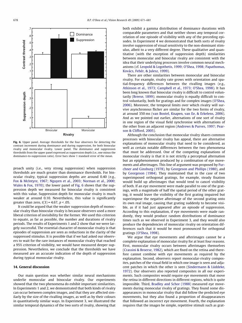
We analysed the mean thresholds for the four observers using atwo-way, within-subjects ANOVA. This found both main effects(rivalry type: monocular vs. binocular; and rivalry phase: domi-nance vs. suppression) to be significant, but critically there wasan interaction between them, F(1,3) = 21.12, p < .05. The thresh-olds are shown in the upper panel of Fig. 6. Suppression depthsare shown in the lower panel of Fig. 6. Suppression depth is calcu-lated by subtracting from unity the ratio of the dominance thresh-old to the suppression threshold. A suppression depth of zero (i.e.,the complete absence of suppression) would occur if suppressionand dominance thresholds were equal. Suppression depths ap-

0

.1

.2

.3

.4

.5

.6

.7

SuppressionDominance

0

.1

.2

.3

.4

Binocular MonocularRivalry

Con

tras

t thr

esho

ldSu

ppre

ssio

n de

pth

Fig. 6. Upper panel. Average thresholds for the four observers for detecting thecontrast increment during dominance and during suppression, for both binocularrivalry and monocular rivalry. Lower panel. The dominance and suppressionthresholds from the upper panel expressed as suppression depth (i.e., one minus thedominance-to-suppression ratio). Error bars show 1 standard error of the mean.


proach unity (i.e., very strong suppression) when suppressionthresholds are much greater than dominance thresholds. For bin-ocular rivalry, typical suppression depths are around 0.40 (e.g.,Fox & McIntyre, 1967; Nguyen et al., 2003; Norman et al., 2000;Wales & Fox, 1970); the lower panel of Fig. 6 shows that the sup-pression depth we measured for binocular rivalry is consistentwith this value. Suppression depth for monocular rivalry is muchweaker at around 0.10. Nevertheless, this value is significantlygreater than zero, t(3) = 4.67, p < .05.

It could be argued that the weaker suppression depth of monoc-ular rivalry than binocular rivalry is because observers used a moreliberal criterion of invisibility for the former. We used this criterionto equate, as far as possible, the number and durations of rivalryperiods. The results of Experiments 1 and 2 show that we were lar-gely successful. The essential character of monocular rivalry is thatepisodes of suppression are seen as reductions in the clarity of thesuppressed stimulus. It is possible that if we had asked our observ-ers to wait for the rare instances of monocular rivalry that reacheda 95% criterion of visibility, we would have measured deeper sup-pression. Nevertheless, we conclude that the thresholds we havemeasured are an accurate indication of the depth of suppressionduring typical monocular rivalry.

14. General discussion

Our main question was whether similar neural mechanismsunderlie monocular and binocular rivalry. Our experimentsshowed that the two phenomena do exhibit important similarities.In Experiments 1 and 2, we demonstrated that both kinds of rivalrycan occur between complex images, and that they are affected sim-ilarly by the size of the rivalling images, as well as by their coloursin quantitatively similar ways. In Experiment 3, we illustrated thesimilar temporal dynamics of the two sorts of rivalry, showing that

both exhibit a gamma distribution of dominance durations withcomparable parameters and that neither shows any temporal cor-relation of one episode of visibility with any of the preceding epi-sodes. In Experiment 4 we demonstrated that both sorts of rivalryinvolve suppression of visual sensitivity to the non-dominant stim-ulus, albeit to a very different degree. These qualitative and quan-titative (with the exception of suppression depth) similaritiesbetween monocular and binocular rivalry are consistent with theidea that their underlying processes involve common neural mech-anisms (cf. Leopold & Logothetis, 1999; O’Shea, 1998; Papathomas,Kovács, Fehér, & Julesz, 1999).

There are other similarities between monocular and binocularrivalry. For example, rivalry rate grows with orientation and spa-tial-frequency differences between the rivalling images (e.g.,Atkinson et al., 1973; Campbell et al., 1973; O’Shea, 1998). It hasbeen long known that binocular rivalry is difficult to control volun-tarily (Breese, 1899); monocular rivalry is equally difficult to con-trol voluntarily, both for gratings and for complex images (O’Shea,2006). Moreover, the temporal limits over which rivalry will sur-vive asynchronous flicker are similar for the two forms of rivalry,at around 350 ms (van Boxtel, Knapen, van Ee, & Erkelens, 2006).And as we pointed out earlier, alternations of one sort of rivalryin one region of the visual field synchronise with alternations ofthe other from an adjacent region (Andrews & Purves, 1997; Pear-son & Clifford, 2005).

Although the conclusion that monocular rivalry shares commonprocesses with binocular rivalry has appeal, there are alternativeexplanations of monocular rivalry that need to be considered, aswell as certain notable differences between the two phenomenathat must be addressed. One of the competing explanations ofmonocular rivalry is that it is not strictly a perceptual alternationbut an epiphenomenon produced by a combination of eye move-ments and afterimages. This line of argument was proposed by Fur-chner and Ginsburg (1978), by Georgeson and Phillips (1980), andby Georgeson (1984). They maintained that in the case of twosuperimposed orthogonal gratings, for example, steady fixationwould build up afterimages that would tend to cancel visibilityof both. If an eye movement were made parallel to one of the grat-ings, with a magnitude of half the spatial period of the other grat-ing, it would leave the visibility of the first grating impaired butsuperimpose the negative afterimage of the second grating ontoits own real image, causing that grating suddenly to become visi-ble, as if it had just appeared after an episode of suppression.According to this explanation, if eye movements were made ran-domly, they would produce random distributions of dominancetimes such as we observed in Experiment 3, and they would alsoproduce the dependencies of monocular rivalry on orientation dif-ferences such that it would be most pronounced for orthogonalgratings (O’Shea, 1998).

We argue that eye movements and afterimages cannot be acomplete explanation of monocular rivalry for at least four reasons.First, monocular rivalry occurs between afterimages themselves(Crassini & Broerse, 1982), which are fixed on the retina and there-fore cannot combine with eye movements as required by theexplanation. Second, observers report monocular-rivalry compos-ites, patches of the visual field in which one image is seen and adja-cent patches in which the other is seen (Sindermann & Lüddeke,1972). Our observers also reported composites in all our experi-ments. Such composites would require eye movements that movethe retina in different directions in different regions, which is quiteimpossible. Third, Bradley and Schor (1988) measured eye move-ments during monocular rivalry of gratings. They found some dis-appearances in monocular rivalry that did follow the predicted eyemovements, but they also found a proportion of disappearancesthat followed an incorrect eye movement. Fourth, the explanationrequires that the images be simple, repetitive stimuli such as grat-


ings, so that an afterimage can be displaced but still provide amatching overlay of the stimulus that generated it. Experiments1 and 2 showed clearly that monocular rivalry is possible betweencomplex images for which no eye movement can superimpose amatching afterimage.1

Given the shortcomings of this alternative account of monocu-lar rivalry, we conclude that monocular rivalry is indeed a genuineperceptual alternation, similar to binocular rivalry, and not an arte-fact of eye movements or afterimages. Nonetheless, despite thestriking similarities between monocular and binocular rivalry, weelaborate below on three differences between the phenomena.We propose that these differences arise because binocular rivalryinvolves a distributed cortical network entailing both low-leveland high-level processes (Blake & Logothetis, 2002; Freeman, Ngu-yen, & Alais, 2005; Nguyen et al., 2003) whereas monocular rivalryinvolves interactions only at higher levels. We agree with Maieret al. (2005) that monocular rivalry is likely to reflect a higher-levelprocess because it involves global interpretations of the probablenature of the stimulus. Therefore, we propose that monocularand binocular rivalry share common high-level processing whichcan be characterised as interpretative processes (e.g., Alais, O’Shea,Mesana-Alais, & Wilson, 2000; Kovács, Papathomas, Yang, & Fehér,1996). The key distinction, then, between the two types of rivalry isthat binocular rivalry involves additional interocular interactionsat early levels of the visual system.2

The first difference between monocular and binocular rivalrywas observed by Breese (1899) in his seminal study. He recordedthat although binocular rivalry’s episodes of dominance involvedalternations in visibility, monocular rivalry was weaker and usu-ally involved alternations in clarity. Consistent with this, weshowed in Experiment 4 that the magnitude of suppression duringmonocular rivalry is much less than in binocular rivalry. We pro-pose that the marked difference in suppression depth is due tothe different extents of the monocular and binocular rivalry net-works rather than to fundamentally different processes. A modelsimilar to that by Wilson (2003) or by Nguyen et al. (2003) or Free-man (2005) could serve here. Specifically, the same inhibitorymechanisms exist at monocular and at binocular levels: thesesum their effects in binocular rivalry, but the monocular part doesnot participate in monocular rivalry, weakening the suppression.The idea of additive suppression components is consistent with re-cent findings that exclusive visibility during rivalry increases asmore dimensions of stimulus conflict are combined (Knapenet al., 2007).

An important consequence of the notion that monocular rivalryinvolves neural interactions common to the high-level part of thebinocular rivalry network is that monocular rivalry should resem-ble other higher-level rivalries. Here, we review only one: stimulusrivalry, or flicker-and-swap rivalry. Devised by Logothetis, Leopold,and Sheinberg (1996), stimulus rivalry occurs when two rivalimages are swapped between the eyes at around 1.5 Hz, while alsoflickering on and off at around 18 Hz. The key observation is thatobservers report episodes of stable visibility of one of the images

1 The same explanation could also apply to binocular rivalry of gratings. Indeed,van Dam and van Ee (2006) found that saccades changing fixation from oneluminance to the opposite luminance (e.g., from a bright bar to a dark bar) were morelikely to be followed by a binocular-rivalry alternation to that grating than saccadeschanging fixation from one luminance to the same luminance (e.g., from a dark bar toa dark bar). This is not to say that binocular rivalry is an epiphenomenon of eyemovements and afterimages. There is an abundance of evidence similar to that formonocular rivalry, including binocular rivalry with afterimages, binocular rivalrywith complex images, and visibility of composites of the two rival stimuli, showingthat eye movements and afterimages are not necessary for binocular rivalry.

2 Although the term ‘‘monocular rivalry” suggests a low-level process, it is simplybecause it has been misleadingly labelled, prompting Maier et al. (2005) to proposethat monocular rivalry would be more appropriately called ‘‘pattern rivalry”.

that endure for long enough to incorporate several interocularstimulus swaps. Each swap, however, is noticeable as a pulse ofsome sort during a single episode of visibility, showing a similarphenomenal absence of complete suppression in this sort of rivalryas in monocular rivalry. Logothetis et al. proposed that rivalry pro-cess acts on representations of images at a high level of the visualsystem where eye-of-origin information (a low-level property) hasbeen discarded. Recent corroborative evidence for this comes fromPearson, Tadin, and Blake (2007) who showed that transcranialmagnetic stimulation of V1 disrupts conventional binocular rivalrybut has no effect on flicker-and-swap rivalry.

We argue that with eye-of-origin information removed, flicker-and-swap rivalry should be very similar to monocular rivalry.Supporting this, we recently found that suppression depth in thisform of rivalry is also shallow (Bhardwaj, O’Shea, Alais, & Parker,2008), similar to that of monocular rivalry. There are at least threeother similarities between monocular rivalry and flicker-and-swap rivalry phenomena that support our proposal. First, monoc-ular rivalry and flicker-and-swap rivalry do not require that eye-of-origin information be retained (unlike conventional binocularrivalry). Second, flicker-and-swap rivalry is promoted by inter-spersing monocular-rivalry stimuli between the swapping stimuli(Kang & Blake, 2006). Third, flicker-and-swap rivalry and monoc-ular rivalry share some interesting parametric similarities. Bothare enhanced at low contrast (Lee & Blake, 1999) and by makingthe images different colours (Bonneh, Sagi, & Karni, 2001; Logo-thetis et al., 1996). Moreover, Knapen et al. (2007) found thatexclusive visibility in monocular rivalry is similar to that fromflicker-and-swap rivalry over a range of colour differences. Thesesimilarities between monocular rivalry and flicker-and-swap riv-alry are, of course, consistent with our overall conclusion thatall forms of rivalry involve a similar, high-level mechanism. In-deed, Pearson and Clifford (2005) showed that all three types ofrivalry, monocular, binocular, and flicker-and-swap, synchronisetheir alternations when all are presented together in adjacent re-gions of the visual field.

The second major difference between monocular and binocularrivalry, and the hardest to reconcile, is that they are affectedoppositely by contrast (O’Shea and Wishart, 2007). Binocular riv-alry alternation rate increases with increasing contrast of the rivalimages whereas monocular rivalry alternation rate decreases withincreasing contrast. Evidence from imaging and transcranial mag-netic stimulation support the claim that early visual processes arecritical in eliciting binocular rivalry (Lee & Blake, 2002; Pearsonet al., 2007; Polonsky, Blake, Braun, & Heeger, 2000). Becauseearly visual responses depend strongly on the level of stimuluscontrast, exhibiting a graded monotonic response to contrast, itmakes sense that binocular rivalry would be strongly modulatedby contrast. Specifically, because increases in stimulus contrastwould increase the V1 response to the rival stimuli, it is as ex-pected that binocular rivalry should be more vigorous at highcontrast.

What is less obvious is why monocular rivalry would be morevigorous at low contrast. One reason may be that the global inter-pretative processes implied by Maier et al.’s (2005) work on mon-ocular rivalry, and more generally by Leopold and Logothetis’s(1999) review, may be less stable at low contrast. That is, reducedsignal-to-noise ratios and stochastic fluctuations would add con-siderable uncertainty to whether a monocular-rivalry stimulusshould be interpreted as one or two objects, and possibly to thedepth ordering if two objects were signalled. To take Maieret al.’s (2005) real-world example, the bottom of a pond mightbe visible transparently even though the water’s surface may re-flect the image of a tree. In this case, with both aspects of the visualscene imaged at the same retinal location, high contrast wouldfacilitate a transparency interpretation and the correct depth order


because both images would be reliably signalled with little ambi-guity. Low contrast, however, would render the problem more dif-ficult as both interpretations would be potentially valid but thecorrect transparency and order relationship would be hard to makewith poorly visible cues. Under these conditions, an interpretativeprocess with bistable behaviour appears to assume more promi-nence and perceptual alternations result.

The lack of vigorous monocular rivalry at high contrast may bebecause there are robust cues for interpreting the image as stable,such as the visibility of the intersections of contours. It may also bebecause high-level neurons tend to be contrast invariant. That is,their contrast-response functions are much steeper initially witha longer saturated plateau (e.g., Sclar, Maunsell, & Lennie, 1990).A magnetic resonance imaging study (Avidan et al., 2002) showedsteeper contrast-response functions in human subjects along theventral visual pathway from V1 through V2, V4/V8, and LO. Be-cause of this tendency towards early saturating contrast-responsecurves, there is no reason to expect that a high-level monocularrivalry process should behave more vigorously at high contrast. In-deed, it would be mainly at low contrast, before reliable responsesare elicited, that a high-level interpretive process would be leaststable.

The third major difference between monocular and binocularrivalry is that they are potentially affected oppositely by disparity.Knapen et al. (2007) have shown that monocular rivalry increasesas two monocular-rivalry gratings are given different disparities tomake them appear to be at different depths. Shimojo and Nakay-ama (1994) and have shown that binocular rivalry decreases byadding disparities. Knapen et al. argued from their results thatmonocular rivalry and binocular rivalry are nevertheless similar,in that the strength of rivalry is determined by the difference be-tween two stimuli in their component features: adding disparityto monocular-rivalry stimuli increases their difference whereasadding disparity to binocular-rivalry stimuli decreases the amountof interocular conflict between them. Knapen et al.’s approach,although from a different direction to ours, comes to a similar con-clusion: that monocular rivalry and binocular rivalry are similarprocesses aimed at resolving ambiguity in visual inputs.

15. Conclusion

In summary, we have shown several qualitative and quantita-tive similarities between monocular and binocular rivalry. Both oc-cur between complex images, both are similarly affected by theimages’ size and colour, both involve fluctuations in image visibil-ity that are random and sequentially independent, and both in-volve suppression of visual sensitivity to the non-dominantimage. We propose that both sorts of rivalry are mediated by acommon high-level mechanism for resolving ambiguity (Alais,O’Shea, Mesana-Alais, & Wilson, 2000; Kovács et al., 1996; Leopold& Logothetis, 1999; Maier et al., 2005), although this process can-not be the primary driver in the case of binocular rivalry, whichmust be initiated by mutually inhibitory interactions between neu-rons retaining eye-of-origin information in early cortex. This high-level process for ambiguity resolution probably exerts a modula-tory influence on binocular rivalry, exerting its influence via feed-back for such things as coordinating local rivalry processes intocoherently rivalling global images (Alais & Melcher, 2007), whereasit is more likely to be the primary driver of monocular rivalry.

Acknowledgments

We are grateful to Frank Tong for allowing us to use his stimulifor Experiment 2, to Janine Mendola for helpful discussion, and toUrte Roeber for help with figures.

References

Alais, D., & Blake, R. (Eds.). (2005). Binocular rivalry. Boston: MIT Press.Alais, D., & Melcher, D. (2007). Strength and coherence of binocular rivalry depends

on shared stimulus complexity. Vision Research, 47, 269–279.Alais, D., O’Shea, R. P., Mesana-Alais, C., & Wilson, I. G. (2000). On binocular

alternation. Perception, 29, 1437–1445.Andrews, T. J., & Purves, D. (1997). Similarities in normal and binocularly rivalrous

viewing. Proceedings of the National Academy of Sciences of the United States ofAmerica, 94, 9905–9908.

Atkinson, J., Fiorentini, A., Campbell, F. W., & Maffei, L. (1973). The dependence ofmonocular rivalry on spatial frequency. Perception, 2, 127–133.

Avidan, G., Harel, M., Hendler, T., Ben-Bashat, D., Zohary, E., & Malach, R. (2002).Contrast sensitivity in human visual areas and its relationship to objectrecognition. Journal of Neurophysiology, 87, 3102–3116.

Beloff, H., & Beloff, J. (1959). Unconscious self-evaluation using a stereoscope.Journal of Abnormal & Social Psychology, 59, 275–278.

Bhardwaj, R., O’Shea, R. P., Alais, D., & Parker, A. (2008). Probing visualconsciousness: Rivalry between eyes and images. Journal of Vision, 8(11,2),1–13.

Blake, R., & Camisa, J. (1979). On the inhibitory nature of binocular rivalrysuppression. Journal of Experimental Psychology: Human Perception andPerformance, 5, 315–323.

Blake, R., & Fox, R. (1974). Binocular rivalry suppression: Insensitive to spatialfrequency and orientation change. Vision Research, 14, 687–692.

Blake, R., Fox, R., & Westendorf, D. (1974). Visual size constancy occurs afterbinocular rivalry. Vision Research, 14, 585–586.

Blake, R., & Logothetis, N. (2002). Visual competition. Nature Reviews Neuroscience,3, 1–12.

Blake, R., & O’Shea, R. P. (2009). Binocular rivalry. In L. R. Squire (Ed.). Encyclopediaof Neuroscience (Vol. 2, pp. 179–187). Oxford: Academic Press.

Bonneh, Y., Sagi, D., & Karni, A. (2001). A transition between eye and object rivalrydetermined by stimulus coherence. Vision Research, 41, 981–989.

Bonneh, Y. S., Cooperman, A., & Sagi, D. (2001). Motion-induced blindness in normalobservers. Nature, 411, 798–801.

Boutet, I., & Chaudhuri, A. (2001). Multistability of overlapped face stimuli isdependent upon orientation. Perception, 30, 743–753.

Bradley, A., & Schor, C. (1988). The role of eye movements and masking inmonocular rivalry. Vision Research, 28, 1129–1137.

Brainard, D. H. (1997). The psychophysics toolbox. Spatial Vision, 10, 433–436.Brascamp, J. W., van Ee, R., Pestman, W. R., & van den Berg, A. V. (2005).

Distributions of alternation rates in various forms of bistable perception. Journalof Vision, 5, 287–298.

Breese, B. B. (1899). On inhibition. Psychological Monographs, 3, 1–65.Breese, B. B. (1909). Binocular rivalry. Psychological Review, 16, 410–415.Campbell, F. W., Gilinsky, A. S., Howell, E. R., Riggs, L. A., & Atkinson, J. (1973). The

dependence of monocular rivalry on orientation. Perception, 2, 123–125.Campbell, F. W., & Howell, E. R. (1972). Monocular alternation: A method for the

investigation of pattern vision. Journal of Physiology, 225, 19P–21P.Chalmers, D. (1995). Facing up to the problem of consciousness. Journal of

Consciousness Studies, 2, 200–219.Crassini, B., & Broerse, J. (1982). Monocular rivalry occurs without eye movements.

Vision Research, 22, 203–204.Crick, F., & Koch, C. (1995). Are we aware of neural activity in primary visual cortex?

Nature, 375, 121–123.Einhäuser, W., Stout, J., Koch, C., & Carter, O. (2008). Pupil dilation reflects

perceptual selection and predicts subsequent stability in perceptual rivalry.PNAS, 105, 1704–1709.

Engel, E. (1956). The role of content in binocular resolution. American Journal ofPsychology, 69, 87–91.

Field, D. J. (1994). Scale-invariance and self-similar ‘wavelet’ transforms: Ananalysis of natural scenes and mammalian visual scenes. In M. Farge, J. C. R.Hunt, & J. C. Vassilicos (Eds.), Wavelets, fractals, and fourier transforms(pp. 151–193). Oxford: Clarendon Press.

Fox, R., & Check, R. (1972). Independence between binocular rivalry suppressionduration and magnitude of suppression. Journal of Experimental Psychology, 93,283–289.

Fox, R., & Herrmann, J. (1967). Stochastic properties of binocular rivalry alterations.Perception & Psychophysics, 2, 432–436.

Fox, R., & McIntyre, C. (1967). Suppression during binocular fusion of complextargets. Psychonomic Science, 8, 143–144.

Freeman, A. W., Nguyen, V. A., & Alais, D. (2005). The nature and depth of binocularrivalry suppression. In R. Blake & D. Alais (Eds.), Binocular rivalry (pp. 47–62).Cambridge, MA: MIT Press.

Freeman, A. W. (2005). Multistage model for binocular rivalry. Journal ofNeurophysiology, 94, 4412–4420.

Furchner, C. S., & Ginsburg, A. P. (1978). ‘‘Monocular rivalry” of a complexwaveform. Vision Research, 18, 1641–1648.

Galton, F. (1907). Inquiries into human faculty and its development. London: Dent.Georgeson, M. A. (1984). Eye movements, afterimages and monocular rivalry. Vision

Research, 24, 1311–1319.Georgeson, M. A., & Phillips, R. (1980). Angular selectivity of monocular rivalry:

Experiment and computer simulation. Vision Research, 20, 1007–1013.Gross, C. G., Bender, D. B., & Rocha-Miranda, C. E. (1969). Visual receptive fields of

neurons in inferotemporal cortex of the monkey. Science, 166, 1303–1306.


Handley, M., Bevin, M., & O’Shea, R. P. (2005). User guide for the ocular dominanceexperiment 2.21. Dunedin: Department of Psychology, University of Otago.

Hollins, M., & Leung, E. H. L. (1978). The influence of colour on binocular rivalry. In C.Armington, J. Krauskopf, & B. Wooten (Eds.), Visual psychophysics and physiology. Avolume dedicated to Lorrin Riggs (pp. 181–190). New York: Academic Press.

Kang, M.-S., & Blake, R. (2006). How to enhance the incidence of stimulus rivalry.Journal of Vision, 6(6), 46a [Abstract].

Kitterle, F., & Thomas, J. (1980). The effects of spatial frequency, orientation, andcolour upon binocular rivalry and monocular pattern alternation. Bulletin of thePsychonomic Society, 16, 405–407.

Knapen, T., Kanai, R., Brascamp, J., van Boxtel, J., & van Ee, R. (2007). Distance infeature space determines exclusivity in visual rivalry. Vision Research, 47,3269–3275.

Kovács, I., Papathomas, T. V., Yang, M., & Fehér, Á. (1996). When the brain changesits mind: Interocular grouping during binocular rivalry. Proceedings of theNational Academy of Sciences of the United States of America, 93, 15508–15511.

Lee, S.-H., & Blake, R. (2002). V1 activity is reduced during binocular rivalry. Journalof Vision, 2, 618–626.

Lee, S. H., & Blake, R. (1999). Rival ideas about binocular rivalry. Vision Research, 39,1447–1454.

Leopold, D. A., & Logothetis, N. K. (1999). Multistable phenomena: Changing viewsin perception. Trends in Cognitive Sciences, 3(7), 254–264.

Levelt, W. J. M. (1967). Note on the distribution of dominance times in binocularrivalry. British Journal of Psychology, 58, 143–145.

Levelt, W. J. M. (1968). On binocular rivalry. The Hague, Netherlands: Mouton.Logothetis, N. K., Leopold, D. A., & Sheinberg, D. L. (1996). What is rivalling during

binocular rivalry? Nature, 380, 621–624.Lumer, E. D., Friston, K. J., & Rees, G. (1998). Neural correlates of perceptual rivalry

in the human brain. Science, 280, 1930–1934.Maier, A., Logothetis, N. K., & Leopold, D. A. (2005). Global competition dictates local

suppression in pattern rivalry. Journal of Vision, 5, 668–677.Mapperson, B., & Lovegrove, W. (1984). The dependence of monocular rivalry on

spatial frequency: Some interaction variables. Perception, 13, 141–151.Meng, M., & Tong, F. (2004). Can attention selectively bias bistable perception?

Differences between binocular rivalry and ambiguous figures. Journal of Vision,4, 539–551.

Necker, L. A. (1832). Observations on some remarkable optical phenomena seen inSwitzerland; and on an optical phenomenon which occurs on viewing a figureof a crystal or geometrical solid. The London and Edinburgh PhilosophicalMagazine and Journal of Science, 1(5), 329–337.

Nguyen, V. A., Freeman, A. W., & Alais, D. (2003). Increasing depth of binocularrivalry suppression along two visual pathways. Vision Research, 43, 2003–2008.

Norman, H. F., Norman, J. F., & Bilotta, J. (2000). The temporal course of suppressionduring binocular rivalry. Perception, 29, 831–841.

O’Shea, R. P. (1998). Effects of orientation and spatial frequency on monocular andbinocular rivalry. In N. Kasabov, R. Kozma, K. Ko, R. O’Shea, G. Coghill, & T.Gedeon (Eds.), Progress in connectionist-based information systems: Proceedings ofthe 1997 international conference on neural information processing and intelligentinformation systems (pp. 67–70). Singapore: Springer Verlag.

O’Shea, R. P. (2006). Control of binocular rivalry and of pattern alternation.Australian Journal of Psychology, 58(Suppl.), 87 [Abstract].

O’Shea, R. P., Alais, D., & Parker, A. (2005). The depth of monocular-rivalrysuppression. Australian Journal of Psychology, 57(Suppl.), 66 [Abstract].

O’Shea, R. P., Alais, D., & Parker, A. (2006). The depth of suppression duringmonocular rivalry and binocular rivalry. Perception, 35(Suppl.), 9 [Abstract].

O’Shea, R. P., & La Rooy, D. J. (2004). Monocular and binocular rivalry with compleximages. Australian Journal of Psychology, 56(Suppl.), 130 [Abstract].

O’Shea, R. P., Sims, A. J. H., & Govan, D. G. (1997). The effect of spatial frequency andfield size on the spread of exclusive visibility in binocular rivalry. VisionResearch, 37, 175–183.

O’Shea, R. P., & Wishart, B. (2007). Contrast enhances binocular rivalry and retardsmonocular rivalry. Australian Journal of Psychology, 59(Suppl.), 51–52 [Abstract].

Papathomas, T. V., Kovács, I., Fehér, A., & Julesz, B. (1999). Visual dilemmas:Competition between the eyes and between percepts in binocular rivalry. In Z.

Pylyshyn & E. LePore (Eds.), What is cognitive science? (pp 263–294). MaldenMA: Basil Blackwell.

Pearson, J., & Clifford, C. W. G. (2005). When your brain decides what you see:Grouping across monocular, binocular, and stimulus rivalry. PsychologicalScience, 16, 516–519.

Pearson, J., Tadin, D., & Blake, R. (2007). The effects of transcranial magneticstimulation on visual rivalry. Journal of Vision, 7, 1–11.

Pelli, D. G. (1997). The VideoToolbox software for visual psychophysics:Transforming numbers into movies. Spatial Vision, 10, 437–442.

Polonsky, A., Blake, R., Braun, J., & Heeger, D. J. (2000). Neuronal activity in humanprimary visual cortex correlates with perception during binocular rivalry.Nature Neuroscience, 3, 1153–1159.

Rauschecker, J. P., Campbell, F. W., & Atkinson, J. (1973). Colour opponent neuronesin the human visual system. Nature, 245, 42–43.

Rubin, E. (1915). Visuell Wahrgenommene Figuren. Copenhagen: GyldenalskeBoghandel.

Rubin, N. (2003). Binocular rivalry and perceptual multi-stability. Trends inNeurosciences, 26, 289–291.

Ruderman, D. L., & Bialek, W. (1994). Statistics of natural images: Scaling in thewoods. Physical Review Letters, 73, 814–817.

Sclar, G., Maunsell, J. H. R., & Lennie, P. (1990). Coding of image contrast in centralvisual pathways of the macaque monkey. Vision Research, 30, 1–10.

Sheinberg, D. L., & Logothetis, N. K. (1997). The role of temporal cortical areas inperceptual organization. Proceedings of the National Academy of Sciences of theUnited States of America, 94, 3408–3413.

Shimojo, S., & Nakayama, K. (1994). Interocularly unpaired zones escape localbinocular matching. Vision Research, 34, 1875–1881.

Sindermann, F., & Lüddeke, H. (1972). Monocular analogues to binocular contourrivalry. Vision Research, 12, 763–772.

Thomas, J. (1978). Binocular rivalry: The effects of orientation and pattern colorarrangement. Perception & Psychophysics, 23, 360–362.

Tong, F., Nakayama, K., Vaughan, J. T., & Kanwisher, N. (1998). Binocular rivalry andvisual awareness in human extrastriate cortex. Neuron, 21, 753–759.

van Boxtel, J. J., Knapen, T., van Ee, R., & Erkelens, C. J. (2006). Exploring theparameter space of stimulus rivalry. Perception, 35(Suppl.), 32.

van Boxtel, J. J. A., van Ee, R., & Erkelens, C. J. (2007). Dichoptic masking andbinocular rivalry share common perceptual dynamics. Journal of Vision, 7(14, 3),1–11.

van Dam, L. C. J., & van Ee, R. (2006). Retinal image shifts, but not eye movementsper se, cause alternations in awareness during binocular rivalry. Journal ofVision, 6, 1172–1179.

Wade, N. J. (1975). Monocular and binocular rivalry between contours. Perception, 4,85–95.

Wade, N. J. (1996). Descriptions of visual phenomena from Aristotle to Wheatstone.Perception, 25, 1137–1175.

Wales, R., & Fox, R. (1970). Increment detection thresholds during binocular rivalrysuppression. Perception & Psychophysics, 8, 90–94.

Wallach, H., & O’Connell, D. N. (1953). The kinetic depth effect. Journal ofExperimental Psychology, 45, 205–217.

Watson, A. B., & Pelli, D. G. (1983). QUEST: A Bayesian adaptive psychometricmethod. Perception & Psychophysics, 33, 113–120.

Wheatstone, C. (1838). Contributions to the physiology of vision—Part the first. Onsome remarkable, and hitherto unobserved, ph�nomena of binocular vision..Philosophical Transactions of the Royal Society of London, 128, 371–394.

Wilson, H. R. (2003). Computational evidence for a rivalry hierarchy in vision.Proceedings of the National Academy of Sciences of the United States of America,100, 14499–14503.

Wilson, H. R., Blake, R., & Lee, S. H. (2001). Dynamics of traveling waves in visualperception. Nature, 412, 907–910.

Wilson, H. R., Krupa, B., & Wilkinson, F. (2000). Dynamics of perceptual oscillationsin form vision. Nature Neuroscience, 3, 170–176.

Yoshor, D., Bosking, W. H., Ghose, G. M., & Maunsell, J. H. (2007). Receptive fields inhuman visual cortex mapped with surface electrodes. Cerebral Cortex, 17,2293–2302.

monocular rivalry exhibits three hallmarks of binocular rivalry: evidence for common processes

Documents