momentum distribution of nucleons in nuclear matter
TRANSCRIPT
Nuclear Physics A427 (1984) 473492 @ North-Holland Publishing Company
MOMENTUM DISTRIBUTION OF NUCLEONS
IN NUCLEAR MATTER+
S. FANTONI
Dipartimento di Fisica dell’ Uniuersita, Pisa, Italy
and
Zstituro Nazionale di Fisica Nucleare, Piss, Italy
and
V.R. PANDHARIPANDE
Department of Physics, University of Illinois at Urbana-Champaign, I1 10 West Green Street, Urbana,
IL 61801, USA
Received 19 December 1983 (Revised 13 March 1984)
Abstract: We calculate the momentum distribution n(k) of nucleons in nuclear matter from a realistic hamiltonian. First the n(k) is calculated from a variational wave function containing central, spin, isospin, tensor and spin-orbit pair correlations. The non-central correlations are found to give the major part of the deviation of n(k) from the f3( k, - k) of a Fermi gas. Next we use second-order correlated-basis perturbation theory to study the effect of correlated 2p2h admixtures in the ground state. These admixtures give significant corrections to the variational n(k), particularly in the region k - k,. They are necessary to obtain the correct behavior of n( k - kF). The discontinuity of n(k) at k = kF is found to be 0.7 and its relations to the effective mass, the one-particle Green function and the difference between charge densities of “‘Pb and *05Tl are discussed. The density dependence of n(k) is studied, and the n( k/k,) is found to be relatively insensitive to density in the region
P =&Jo to PO.
1. Introduction
The occupation probability n(k) of states with momentum k is an interesting
property of quantum liquids; it can be measured by deep-inelastic scattering experi-
ments. In ideal Fermi gas the probability is simply one for k< k, and zero for
k > kF Interactions induce correlations in the wave function which deplete n( k < kF)
and increase n(k > kF). Thus the deviation of n(k) from O( kF- k) is indicative of
the strength of correlations.
The natural choice for the single-particle states to describe nuclear wave functions
is shell-model orbits labelled with quantum numbers n, 1 and j. In a simple shell
model one expects the occupation probabilities of occupied orbits to be one.
However, in pickup or knockout lS2) reactions it is found to be less than one indicating
the presence of correlations. In a recent experiment ‘) the difference between the
+ Work supported in part by NSF grant PHYSl-21399 and NATO grant N.0453/82.
413
474 S. Fantoni, KR. Pandharipande / Momentum distribution
charge distributions of ‘06Pb and *“Tl was measured and found to be -0.6 times the charge distribution of a 3s,,* proton and a smooth background. This measurement indicates that the occupation probability of 3s I,* orbit changes by less than one in going from *OsPb to *05Tl.
In the present work we calculate n(k) in nuclear matter. In sect. 2 the nuclear matter wave function is approximated by the variational wave function
I%)=(9 ii +M, 1>J=l
(1.1)
and the expectation value of aLak is calculated. The SV are pair-correlation operators,
(1.2)
o;=‘L 1 , tTi ’ Tj) 9 tai ’ uj) 9 (ai * uj)(Ti ’ Tji) 9
Sij, Sij(Ti' Tj) 2 L'S, L * S(Ti * Tj) 3 (1.3)
Y is the symmetrizer, and IO,) the Fermi-gas wave function. The f”( rii) are para- meterized in a convenient way 4), and the values of the parameters are determined by minimizing the energy expectation value. The Urbana vi4 +TNI interaction 5, is used in this work. Studies of the nuclear matter equation of state ‘) and single-particle (optical) potential 6*7) with this interaction have been reported earlier. We use the variational wave function reported in ref. “).
The results of this “variational” calculation are not very satisfactory, particularly at k - kp It was found in ref. ‘) that the IO,) is too simple to give the single-particle energies correctly at k - kF, and hence we should not expect the variational calcula- tion of n (k - kF) to be adequate. In sect. 3 the wave function is generalized by using perturbation theory in a correlated basis (CBF), and the n(k) is calculated by retaining the variational and second-order CBF terms. This n(k) has the correct physical behavior 8,9). The connections between n(k), the one-particle Green func- tion lo) and the effective mass ‘l) are discussed in sect. 4. In sect. 5 we report II as a function of the single-particle energy, and also comment upon other effects that may influence the occupation numbers in finite nuclei.
2. Variational calculation of n(k)
In an isotropic liquid the n(k) depends only upon lk\, and it is conveniently written as the Fourier transform of the one-body density matrix. n(r,, r,,). In homogeneous liquids n(r,, rlt) depends only upon the distance rll,= (r, - r,& and
n,(k) = I dr e-ik’rllxv( r, ,,) , (2.1)

S. ~antoni, K R, Pand~~ipa~de f momentum dist~bution 47s
dr, * * - dr, %XXI, x2, . - - , XA) ~dxl,, x2, . . . , ~4 n,(r,,,) =+A
I dr, - . * dr, 1 pvi2
Here WV is the variational wave function IO,) in coordinate space,
(2.2)
P”(X 1,..., xJ=(y” $ij, %)dIJ @*hJ, (2.3)
@,(x,) are single-particle plane waves, and x, denotes the position r, and the spin-isospin of particle (Y. The f in eq. (2.2) takes into account the spin-isospin degeneracy.
The calculation of n,(k) is technically involved, and most of its details are given in the appendices. A cluster expansion of n,( rl ,‘) is made, and the important diagrams contributing to it are summed up with the help of Fe~i-hype~etted-chain and single-operator-chain summation techniques ‘2V13). In this section we give only the results and discuss the normalization and kinetic-energy sum rules.
Table 1 gives the calculated values of n,(k) and nd( k) in equilibrium nuclear matter ( kF = 1.33 fm-‘, p. = 0.16 fm-“). The nd( k) is obtained by setting all the fp” (spin-isospin correlations) in the correlation operator S$ equal to zero. The n:(k) is much closer to the Fermi gas O(kF- k) than the n,(k), suggesting that the spin-isospin correlations are more relevant than Jastrow correlations in nuclear matter.
The no~alization sum rule states that
and follows from particle conservation. It is satisfied when n,( rI ,, --, 0) = $p, which follows directly from eq. (2.2). In general, however, eq. (2.4) is not exactly satisfied when chain summation techniques are used to calculate n,(r,r), and the sum over elementary diagrams is truncated. For example when n,(r,,~) is calculated with the FHNC equations, the So in liquid 3He is found r4) to be 1.15, indicating b 15%
TABLE 1
The variational n,(k) in equilibrium nuclear matter, with and without spin-isospin correlations
k (fm-‘) h,(k) n:(k)
0.07 0.90 0.97 1.26 0.90 0.97 1.40 0.0081 0.0023 4.06 0.0006 0.0003

476 S. Fantoni, V.R. Pandha~pa~de / ~orne~rurn distribution
TABLE 2
Contributions to n(h) ~100
h (fm-‘) l--n,(h) h(h) W(h) W(h),,, l--n,(h)
0.297 10.2 -1.02 -2.2 -2.5 13.4 0.515 10.1 -1.26 -2.5 -2.6 13.9 0.665 10.0 -1.50 -2.5 -2.9 14.0 0.787 9.9 -1.79 -2.9 -3.0 14.5 0.892 9.8 -2.15 -3.0 -3.3 15.0 0.986 9.7 -2.55 -3.2 -3.5 15.5 1.072 9.7 -3.02 -3.4 -3.7 16.1 1.152 9.6 -3.63 -3.7 -4.0 16.9 1.226 9.6 -4.44 -4.0 -4.2 18.0 1.296 9.5 -5.63 -4.3 -4.5 19.4
error in the FHNC summation. In nuclear matter however, S, is found to be 1.003 which suggests that FHNC/SOG summation of n,(r,,<) diagrams may be adequate.
The kinetic energy can be calculated from the n,(k),
h2 4 E”,/A=--
2mp (271)3 dk k*n,(k) , (2.51
and directly by cluster expansion of the expectation value of the kinetic-energy operator ‘). The value of Ex obtained from the n,(k) is 37.5 MeV which is quite close to the expectation value “) of 38.7 MeV. Hence it is likely that the present calculation of n,(k) is accurate to few percent.
The calculated values of n,(k) are tabulated in tables 2 and 3 for hole and particle states, respectively.
TABLE 3
Contribution to n(p) x 100
p Urn-‘) %(lJ) WP) W(P)
1.363 0.81 3.80 1.6 6.2
1.501 0.84 1.83 1.3 4.0
1.646 0.86 0.97 1.02 2.85
1.797 0.86 0.54 0.78 2.18
1.955 0.83 0.30 0.57 1.70
2.120 0.77 0.17 0.39 1.33
2.291 0.70 0.093 0.25 1.04
2.469 0.61 0.052 0.15 0.81
2.654 0.52 0.03 I 0.085 0.64
2.845 0.41 0.019 0.043 0.47
3.39 0.18
4.06 0.059
4.99 0.012
6.05 0.0014
S. Fantoni, V.R. Pundha~~~de ,t ~o~enfu~ disf~bution
3. Perturbative correction
477
As stated in the introduction, we+expect that the present variational calculation of n( k‘) will not be adequate in the region of k - kF. The correlation operator Sp n 9 is too simple to realistically represent the correlation of particles close to the Fermi surface. In correlated basis (CBF) perturbation theory the ground state is considered as a superposition of normalized but non-o~hogonal states given by
Ii)= 9 II sI4(ni(k)))
(4(%(k))I(Y II p+)(y II Y”)14(a(k)))“2 ’ (3.1)’
Here I+(ni(k))) are Fermi-gas states with occupation numbers ni( k). We follow the notation of ref. ‘) in which Ii) is denoted by lh,hz - - . p1p2 - * ->, where the h,, hz. - . ,
PIIPZ’ - - specify the holes and particles in q(k). The unno~alized wave function of the ground state, obtained in second-order
perturbation theory restricted to 2p2h intermediate states, is given by
102)=10)+a~~2(Y(hl~ZP1PZ)l~lh*P1PZ), (3.2)
PIP2
4hh2PIP2) = h~2PIPzl~-GolO)
e’(h) t-e’(h) - e’(Pd - e’(P2) ’ (3.3)
Here e’(k) are variational single-particle energies I’), and ti& the variational ground-state energy. The q(k) in this second-order approximation is given by
n (k) _ OkhWlOz> 2 -
@,lO,> ’ (3.4)
and only terms of order ar* need to be kept in its evaluation. Moreover, nondiagonal matrix elements of the unit or n(k) operators are considered to be of order Q.
With straightfo~ard algebra we obtain n,(h) as
n2(h) = K4~(w-Q -4 (
h 2 ~p*K+wl~~2P* P2bChh2PI P2)
+c.c. +w,Pl Pzl4Wh2P, P*b2W2P1 P2) I
+a h,h$gh) {{o~~(~~~~~~*P~ P*)~(~,~*P~ P2) fC.C*
Prf??
-a<eom c {(Olh*h2p,p,)a(hlhzPlP*) +c*c. +~2(M2P,P2)I~ (3.5) hhz PIP2
It is possible to simplify (3.5) with several reasonable approximations. First the diagonal elements of n(h) in states /i) having ni(h) = 1, for example IO),
418 S. Fantoni, V. R. Pandharipande / Momentum distribution
(hlhl(#h)plp2) etc., are given by n,(h) = 0.9. Thus in terms of order (Y* we can approximate them by one. For the same reason terms of order a2 containing matrix elements such as (hh2p,p21n(h)lhh2p,p2) may be neglected.
Second, we evaluate the nondiagonal elements of n(h) in the two-body cluster approximation:
(3.6)
(hh2p,P2(n(h)10)~(p,p219,2-11hh2)2,+terms of order (.S2-l)2, (3.7)
where (I ()2B denotes antisymmetrized two-body matrix elements. We find that the matrix elements of (.@, - 1) are approximately twice those of (.P12- 1) indicating that the ( $,2 - 1)2 terms in (3.7) may be neglected. Using these approximations we
get
n,(h) = n,(h) +&x,(h) +6$(h), (3.8)
an,(h) = -; C a2(hh,p,p,), (3.9) h,pl PZ
fin;(h) -f C {((hh#- llp,p,)zr(hh,l~2- llp,pdmMhh2p,pA +c.cJ ham p2
=-f C (hh#- llp,p,b(hh,p,pJ +c.c. hzpl PZ
(3.10)
A similar calculation of n2(p) gives
n,(p) = n”(P) +sn,(P) +W(p) 9 (3.11)
f3n,(p) =i C a2hh2w2), h,hzm
(3.12)
an;(p) -f C (h,h2/8- lIpp,),,4h,h,pp,) +c.c. (3.13) h,h,p,
We note that &r,(k) is the well-known second-order contribution to n(k) in ordinary (i.e. orthogonal basis) perturbation theory, while &r:(k) represents the nonorthogon- ality correction. The present calculation of L%;(k) is crude, but it contributes only -20 to 30% of the total (n(k) - 6(kF- k)). There should be -10% corrections to Sn2( k) from deviation of n( h)( n( p)) in the correlated states lhh2pl p2) (Ih, h2pp2)) from zero (one).
The numerical calculations were done following the methods outlined in refs. 6S7). The (Y (h, h2p, p2) are calculated approximately by keeping two-body and three-body separable terms in the matrix elements of H-H&,. The results for hole states are given in table 2, while those for the particle states are in table 3. The GnXh)app values in table 2 are calculated with the second eq. (3.10) containing only the matrix elements of (9- l), while &i(h) values are obtained from the first eq. (3.10) having the difference between the matrix elements of ( .Y2 - 1) and (9 - 1). The difference
S. Fantoni, V.R Pandharipande / Momentum distribution 479
between &r;(h) and 6n&(h),,, is due to terms of order (9- l)* that are neglected in eq. (3.7). Both n(h) and n(p) have infinite slopes as h or p + kP This singularity is well known ‘**) and in the present work it comes from the Snl( k); n,(k) and h:(k) have finite slopes as k+ kF from above or below.
We define
x=Ik-k&kF, (3.14)
n(k,-)=n(h+k,), (3.15)
n(k,+) = n(p+ kF) . (3.16)
The n(k- kF) is then given by
n(h-k,)=n(k,-)-Axlnx, (3.17)
n(p-k,)=n(k,+)+Axlnx. (3.18)
The b,(k) is related to the imaginary part of the self-energy Z(h, E > er) and Z (p, E < e,) where eF is the Fermi energy:
Im Z(h, E > eF) =&rx ((OlH-H~lhhzplp2)12S(E +e’(h2)-e’(p,)-e’(p,)), (3.19)
Im Z(p, E < eF) =fC 1(01H-H~olh,h2pp2)12S(E +e’(pz)-e’(h,) -e’(h2)), (3.20)
Sri,(h)) =i I 00 Im 1(h, E)
+ dE(e’(h)-E)2’
dE Im E(P, E)
(e’(p)-E)*’
(3.21)
(3.22)
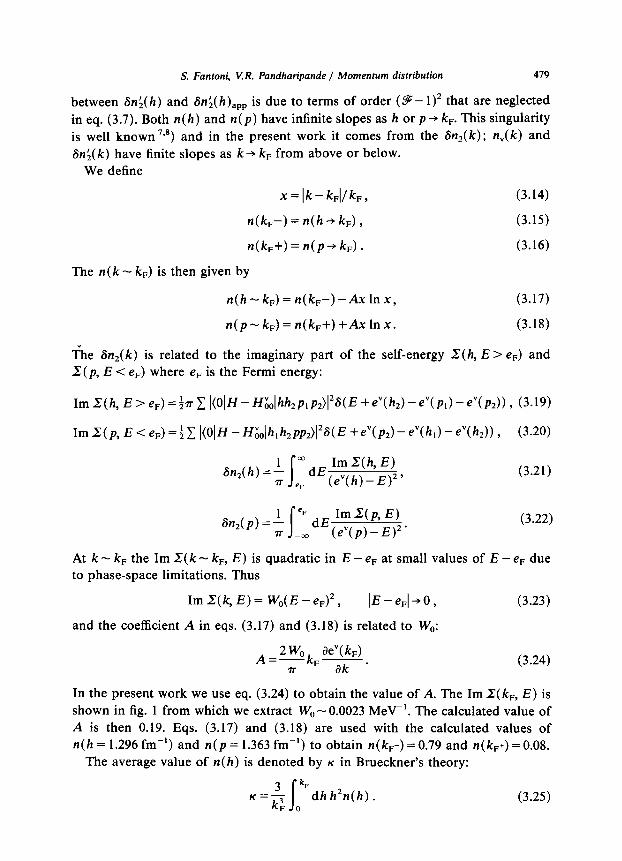
At k - kF the Im Z( k - kF, E) is quadratic in E - eF at small values of E - eF due to phase-space limitations. Thus
Im I( k, E) = W,( E - eF)2 , b-d-,0, (3.23)
and the coefficient A in eqs. (3.17) and (3.18) is related to W,:
2w k ae”(W A=- ~ T F ak ’
(3.24)
In the present work we use eq. (3.24) to obtain the value of A. The Im Z(kF, E) is shown in fig. 1 from which we extract W, - 0.0023 MeV-‘. The calculated value of A is then 0.19. Eqs. (3.17) and (3.18) are used with the calculated values of n(h=1.296fm-‘) and n(p=1.363fmP’) toobtain n(k,-)=0.79and n(k,+)=0.08.
The average value of n(h) is denoted by K in Brueckner’s theory:
3 k, K=x
k I dh k*n(k) . (3.25)
F 0
480 S. Fantoni, V.R. Pandharipande / Momentum distribution
Fig. I. The imaginary part of the self-energy at k = k,, in equilibrium nuclear matter, as a function of
the energy E.
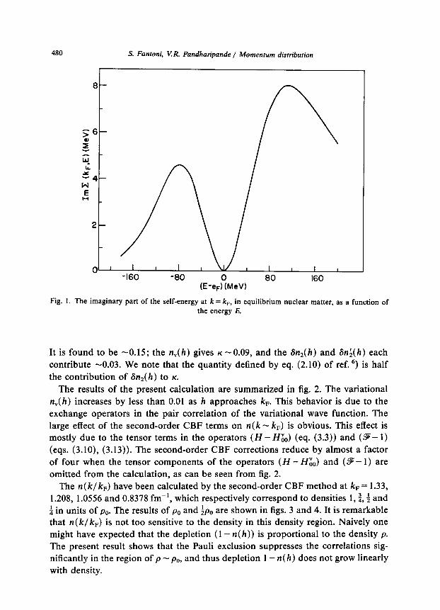
It is found to be -0.15 ; the n,(h) gives K -0.09, and the &r,(h) and &r;(h) each contribute -0.03. We note that the quantity defined by eq. (2.10) of ref. “) is half the contribution of S&(h) to K.
The results of the present calculation are summarized in fig. 2. The variational n,(h) increases by less than 0.01 as h approaches k,. This behavior is due to the exchange operators in the pair correlation of the variational wave function. The large effect of the second-order CBF terms on n(k - kF) is obvious. This effect is mostly due to the tensor terms in the operators (H - H&) (eq. (3.3)) and (9- 1) (eqs. (3.10), (3.13)). The second-order CBF corrections reduce by almost a factor of four when the tensor components of the operators (H - H&J and (9 - 1) are omitted from the calculation, as can be seen from fig. 2.
The n( k/ kF) have been calculated by the second-order CBF method at kF = 1.33, 1.208, 1.0556 and 0.8378 fm-‘, which respectively correspond to densities 1, .& t and a in units of p* The results of p0 and &, are shown in figs. 3 and 4. It is remarkable that n( k/ kF) is not too sensitive to the density in this density region. Naively one might have expected that the depletion (1 - n(h)) is proportional to the density p. The present result shows that the Pauli exclusion suppresses the correlations sig- nificantly in the region of p - po, and thus depletion 1 - n(h) does not grow linearly with density.

S. Fantoni, V R. Pandharipande / Momentum distribution 481
-----w-m-__
-N -Variational
0.88-
0.82 -
z c
0.79 - /
Fig. 2. The occupation probabilities in equilibrium nuclear matter obtained from variational and CBF calculations. The full and broken lines show results of second-aider CBF calculations with and without
tensor operators, respectively.
4. One-particle Green function
The n(k) is related to the one-particle Green function with the well-known lo)
equation
n(k)=& G(k,w)e-‘“‘dw, I
(7+0-). (4.1)
In normal Fermi liquids, the G( k, w) in the region k - k, can be expressed as
G( k, w) = z
ct~-G(k)-iy(k)+~(~~)’ (4.2)
using the Lehmann representation. The two terms in (4.2) refer to the quasi-particle

482 S. Fantoni, V.R. Pandharipande / Momentum distribution
0
0.t ;i c
0
.9-
35-
.0 -
/@ 3 PO
f Fig. 3. The occupation probabilities of hole states in nuclear matter at density pO and $,,.
0.06
Y
= 0.04
0.02
0 I 1 I I I I I
1.5 2 (k/kF)
Fig. 4. The occupation probabilities of particle states in nuclear matter at density pO and f~,,.

S. Fantoni KR. Pu~dharipande / momentum disr~bu~ion 483
pole and background, respectively. From eqs. (4.1) and (4.2) Migdal lo) obtained the relation
Q(n(k,-E)-n(kF+E))=Z (4.3)
between the discontinuity of n(k) at kF and the renormalization constant 2. Our calculation would indicate that 2 - 0.7.
The G(k, w) can also be expressed as
Gfk 0) = 1
w-w,(k)+X*(k,o)’ (4.4)
where X*(/C, w) is the proper self-energy. The o,(k) are free-particle energies ( k2/2m), and the quasiparticle energies (5( k - kF) are given by consistent solutions of
~(k)=~o(k)+Re~(~~(k)).
The renormalization constant 2 is given by I”)
(4.5)
8 Re I(k,o)
aE w=+ ’ k=kF
(4.6)
where E denotes to real part of o. The 2-I appears as a factor in the Landau effective m&s:
(4.7)
and has been called the E-mass by Mahaux and coworkers” ). Our calculations give the E-mass in nuclear matter at k - k, to be - 1.43. If we express the total effective mass m*(k,), found to be -0.81 m in ref. 7), as
m*(k,) = (bare mass) x(K -mass)/Z, (4.8)
the K-mass appears to be 0.57. These values of K- and E-mass are similar to those found by the Libge group 16), except that the K-mass is - 10% too small. It should be noted that neither in theory, nor in practice, does the variational effective mass m*, found to be -0.65m [ref. “)I, equal the K-mass.
5. Conclusions
The momentum distribution n(k) of nucleons in nuclei such as *“Pb may be estimated from that in nuclear matter by using local density approximation. Such a calculation is in progress. However, in some problems it may be more interesting to consider the occupation numbers of shell orbits n(n&). From the present calculation we may expect the n(n@r) of deeply bound orbits to be -0.86.

484 S. Fantoni, VR. Pandharipande / Momentum distribution
0.81-
0.78-
2 c
0.09-
0.06-
-40 -20 20 40
Fig. 5. The occupation prbbability as a function of the single-particle energy e in equilibrium nuclear matter.
The occupation probability of an orbit probably depends most crucially on the
e( nlj7) - eF, where e( n&r) is the single-particle energy. Hence in fig. 5 we have
plotted the n(k) against the single-particle energy e(k) obtained in second-order
CBF calculation ‘).
The n(e) in nuclei may differ from that in nuclear matter due to the coupling of
the single-particle states to the surface vibrations, and pairing. The “‘Pb, where the
pairing effects are small, Gogny 17) has studied the effect of the coupling of single-
particle states to vibrations with the random-phase approximation (RPA). He finds
that BnRPA depends mostly on the e( nlj7) - eF, thus it may be reasonable to discuss
n(e) in finite nuclei. The SnRpA(e) h as a much more rapid variation with e than the
n(e) of fig. 3, and it can decrease the Z-factor ( n(eF-) - n(er+)) by -0.2. The
low-energy single-particle states of nuclei have large widths due to their coupling
with the surface. These correspond to a value 18*19) of W. (eq. (3.23)) of -0.02 MeV-’
instead of the 0.0023 MeV-’ in the present work. It is thus not surprising that the
Sn RPA has a much more rapid variation with e - eF.
We can estimate the differences 6p, between the charge densities of 206Pb and
205Tl crudely by assuming that the occupation of one of the 3sij2 orbits changes
S. Fantoni, VR. Pandharipande / Momentum distribution
from n( eF-) to n ( eF+). This gives
485
Sp, = Zp,(3s,,,) +background , (5.1)
where p,(3~,,~) is the charge density of a proton in 3s,,, orbit, and the background is from the small changes in other occupation numbers. Eq. (5.1) may also be obtained from the approximation (4.2) of the one-particle Green function. From this simple picture we obtain 2 - 0.6 in 208Pb from the experimental data ‘) on &I,. This value of 2 is a little smaller than our estimate of 0.7 in nuclear matter; however, that could be due to surface effects. Secondly, eq. (5.1) may not be very accurate in finite nuclei. The proton Fermi energies of 206Pb and 205Tl are uncertain by several MeV due to shell effects.
Appendix A
CLUSTER EXPANSION OF n,(k)
The power-series method 20) (PS) is applied to expand n,( r, r,). Such an expansion extends, to the present more general case, the expansion given in ref. 12) for the case of a correlated wave function of the Jastrow type.
Both the numerator and the denominator of eq. (2.2) are expanded in powers of the short-ranged functions F’,(rai), Fc(rU), FL”(r,,), FP”(r,) andfP”(r,)fq”(rU), where
FXr,,) =f(ral) - 1 , FC”(r,,) =fp”(rol), (a = 1, 1’)) (A-1)
F’(r,) =f’*(rti)- 1 , FP”‘(r,,) = 2F(ri,l_fp”(ri,), (i,j # 1, 1’) . (A.2)
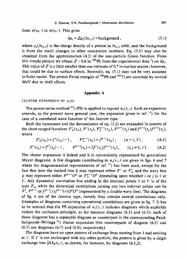
The cluster expansion is linked and it is conveniently represented by generalized Mayer diagrams. A few diagrams contributing to n,(r,,s) are given in figs. 6 and 7 where the diagrammatical representation of ref. 13) has been used, except for the fact that here the dashed line ij may represent either F’ or F’, and the wavy line ij may represent either Fp”Op or FL” Op depending upon whether i or j is 1 or 1’. Any dynamical correlation line ending in the external points 1 or 1’ is of the type F, while the dynamical correlations joining any two internal points can be Fc, Fp” or fp” ( r)fq”( r)OPOq (represented by a double wavy line). The diagrams of fig. 6 are of the Jastrow type, namely they contain central correlations only. Examples of diagrams containing operational correlations are given in fig. 7. It has to be noticed that the PS expansion of n,(r,,.) includes diagrams which explicitly violate the exclusion principle, as for instance diagrams (6.3) and (6.5); each of these diagrams has a separable diagram as counterpart in the corresponding Pand- haripande-Wiringa 13) cluster expansion (the counterparts of diagram (6.3) and (6.5) are diagrams (6.7) and (6.8), respectively).
The diagrams have an open pattern of exchange lines starting from 1 and arriving at 1’. If 1’ is not exchanged with any other particle, the pattern is given by a single exchange line fJ( k,r,,,), as shown, for instance, by diagrams (6.1,2).

486 S. Fantoni, KR Pandharipande / Momentum distribution
i / 4
?i
h-7 ,lL-f+ A
I’ I
6.1 6.2 6.3
,+y ‘t-----T’
6.7 6.8
Fig. 6. Jastrow-type diagrams contributing to n,(k). Diagrams (6.7,8) are counterparts of diagrams (6.3)
and (6.5) if the Pandharipande-Wiringa cluster expansion is used.
j i
r=7 I’ I
7.4
A
j i
I’ I
7.7
k .
E j
I’ I
7.2
j i
n I’ I
7.5
i
A I’ I
7.0
i
A I’ I
7.3
i
A I’ I
7.6
i j
m I’ I
7.9
Fig. 7. SOC diagrams included in the calculation of n,(k).

S. Fanfo~i, KR. Pandha~~ande / ~o~ent~~ di~t~bu~~o~ 487
The cluster expansion of n,(r,,,) is reducible, i.e. there are separable diagrams contributing to it. Separable diagrams are summed up by associating proper vertex corrections with the internal and external points of the connected diagrams. The vertex corrections on the external points 1’ and 1 are characteristic of the cluster expansion of n,(r, ,‘) and they are present even if the operatorial components of the correlation functions are set equal to zero. The diagrams which are separable at I or 1’ are not cancelled since the d~amical correlations ending on 1 or 1’ are of different type from those joining any two internal points. For instance, diagram (6.3) does not cancel diagram (6.2) and the net contribution to n,(k) coming from diagrams (6.1-3) is given by
8(kF-k) 1 +p [ I
dr (2F”,( r) - FC( r)) . 1 (A.3)
The expression in square brackets is the lowest-order evaluation of the vertex correction n to the external points, which is usually named strength factor. The lowest-order cont~bution to n from noncommutivity of correlation operators is associated with diagrams of type (7.1).
In the case of a correlated wave function of the Jastrow type (P” = FL” = 0) 11 is the only vertex correction that has to be considered, and one has 21)
#)(k)‘= rl(J)N(‘)( ,+) . ” (A-4)
Since N’“‘(k) is discontinuous at k = kF this is more conveniently written in the form
N’J’(k) = Gus) +B(k,- keel), (A.5)
where both NY’ and N(dJ’ are continuous functions. In the case of a non-interacting Fermi system one has 7 = N’dJ’( k) = 1 and Nr”( k) = 0. The discontinuous term on the r.h.s. of eq. (AS) is given by the sum of the nodal diagrams in which one or two nodal elements are undressed exchange lines (see, for instance, diagrams (6.1) and (6.4-6)). Diagrams (6.4) and (6.5) do not cancel each other since their dynamical correlations are of different type.
In the more general case of a correlated wave function of the type given in eq. (1.1) the vertex correction on the external points cannot be exactly factored out from n,(k) and one has
n,(k) = TN(k) +A%,(k) , 64.6)
where AiV,,,( k) is due to the commutators of the correlation operators having either 1’ or 1 as common point. For example, diagram (7.1) gives contributions to both
TN(k) and A%,(k). There are also vertex corrections associated with internal points, as in the case
of the point i of diagram (7.2). Such vertex corrections are of the same type as those discussed in sects. 4 and 5 of ref. 13) and have been treated by using the method described there.

488 S. Fantoni, VIR. Pandharipande / Momentum distribution
Appendix B
FHNC/‘SOC EQUATIONS FOR n,(k)
The FHNCf SOC equations for the momentum distribution n,(k) are easily obtained by applying the method described in ref. 13) to extend the FHNC treatment of ref. I’). Let us write the function N(k) appearing in eq. (A.6) in the form
N(k)=N’,J’(k)+N:oC(k)+8(k,-k)[NjiJ’(k)+N~oC(k)], (B.1)
where the contribution coming from Jastrow-type diagrams is separated from that of single operator chain diagrams. The chain diagrams (6.4-6) are the typical diagrams contributing to NY’, which is then given by
NI;“( k) = 1 +2riw, - & +J?f&‘( 1 - r?,) , 03.2)
where the notation of ref. 13) is used and
f= p dr e’k”f(t). (B-3)
The label w stands for a dynamical correlation of type F, The function N?(k) is given by nodal diagrams of the type cc with no undressed exchange lines and the composite diagrams obtained by hypernetting the chain diagrams which contribute to N&J’(k):
r J N’,“(k)=(exp(G,,)-l)(tl-G,,,)-~2,,/(1-~~~), (B.4)
where
Gww(r) = 0(X,, +X,,; Gdw f&w) +0(X,,; G,, +X,,) , VW
&WC = ~(k~-k){l-~~~)(k)}+~~~/(l-~~~~. 03.6)
The nodal functions G,&r) are given by
G,,t r) = C @(X,,r; X,*x + G,,,) , (B.7) X’Y’
for x=d, e and by
G,,,, = 0(X,,; X0 +$) . (B-8)
The composite functions are defined as
X,,=f%;--G,,,d-l, (B-9)
X,,=(.D:,-l)G,, (B.lO)
x,, =$(f”h”,- l)L,, (B.ll)
where J&=exp{GwdI, (B.12)
L, = 4G,, - I( ac,r) . (B.13)
The single-operator chains contribute to lVSoC and the corresponding equations
S. Fantoni, V.R. Pandharipande / Momentum distribution 489
have a similar structure to the above FHNC equations. Diagrams (7.3-6) are examples of diagrams included in N ‘O”(k). In what follows the SOC equations for
Nz°C and Nsoc are given for the case of a correlation operator without L * S
components:
7 Nz°C( k) = ,;, APAP{2&, +kf$L(XP,, + Gsd)
+2kRvJ(l -Xc,)>, (B.14)
N:“‘(k)= -(exp(G,,)-l)G::: + C APAPGL($ - G,,,) exp (G,,) P#l
where
- 2 C ApApri;p,,~w,/( 1 - &) , Pfl
(B.15)
G;, = C C Opqr(X:x’; X& + G$,)M: , X’Y’ P9
(B.16)
G -sot_ WWE --O(kF-k)N;oC(k)+2 C APAPXP,,~,,,,/(l-~~~).
P#l
(B.17)
The nodal functions GP, for x = e or d, are given by
GLx = C C Opq’(Xp,,; X;,, + G;,,)M; , X’Y’ P4
(B.18)
wherez=difx’=y’=dandz=eifx’ory’=e,and
G:, = C Opq’(Xp,,; Aq(Xcc +;L) . P4
(B.19)
The composite functions Xp are defined as
X$=hPhc -GP w w wd ,
XL = KG,, +_f=Llh; - GP,, ,
Xp,, = [hP,&,,M~ +fCGP,]hC, - GP, , where
(B.20)
(B.21)
(B.22)
hp,= f"+fCG$d. (B.23)
The derivation of the FHNC equations for the strength factor is given in ref. ‘*). Here we limit ourselves to give the expression of v(‘) and briefly discuss its extension to include SOC contribution:
where 77 (‘) = exp {2R”‘( w) - R”‘(d)} , (B.24)
@J’(CZ)=p dr{X,,(r)+X (r)} cc<
1 1 --- (2TJ3P 2 I
dk i&d +6,)(&d + Ghd) + c?,d(k, + k,,>, (B.25)

490 S. Fantoni, V.R. Pandharipande / Momentum distribution
with (Y = w, d. The inclusion of single-operator chain diagrams leads to the following expression for 7):
where
T= #‘)( 1 +2RSoC( w) - Rsoc(d)) , (B.26)
Pot(u) = p;, RP((u) =$p I
dr p;, AP{XZd(GEdMPd + GfLM3 +-%,G%Mi?.
(B.27)
The commutator contribution AN,,,(k) appearing in eq. (A.6) comes from diagrams such as (7.1) which have R ‘O’(w) as vertex correction; on the contrary, diagrams such as (7.7) which have a vertex correction of the type RSoC(d) do not give any contribution to AN,,,(k). The two separate parts of diagram (7.1) have f as probability of alternating order, hence AN,,, is given by
with
ANcom,d (k) = f C APApDp,R’( w)&( 1 + X,,zc< 1 -Xc=)) (B.29) p,- 1
AN,,,,Jk) = -(;xp+$ .;, APAPDp,R’(w)
x[GP,,($l-G,,) exp (G,,)-XL,X,J(l --%>I9 03.30)
AG t,E = - e(k, - k)ANm,, +$ C ApApDpJZ’(~)&,~,J(l -X,,) . (B.31) PY> 1
In order to treat exactly the lowest-order cluster terms, diagrams (7.8) and (7.9) have also been included in the present calculation. The contribution of these diagrams is given by
ANeXC( k) = -p I dr e-“” c P.4.4f 1
A’Bpq’( frf”; $I C fdSKapq) 0
+8(kF-k)p dre-“.’ C A’f’fPAqK,,. I P191Z’I
(B.32)
The L - S correlations have also been treated in lowest order, i.e. only diagrams (7.6-9), with the wavy lines representing L - S components, have been taken into account. The corresponding contribution is given by
ANLS(k)=AN:S(k)+B(kF-k)AN;S(k), (B.33)
S. Fantoni, V. R. Pandhoripande / Momentum distribution 491
where
x (11~2~;2/ r12 + 42W fMri2 * rt2) ,
ANY(k)=& dreik”(fb’+6fbfb7-3fhZ) J (B.34)
x(rl’-t$l((k+ r)‘- k2r2)). (B.35)
Neither AN’“’ nor ANLS give contribution to the normalization of n,(k), namely
J dkAN”““(k)= dkAiVLS(k)=O. J (B-36)
References
1) A. Bohr and B. Mottelson, Nuclear structure, vol. I (Benjamin, Reading, Mass., 1969) 2) G. Jacob and T.A.J. Maris, Rev. Mod. Phys. 45 (1973) 6;
J. Mougey, M. Bernheim, A. Bussiere, A. Gitlebert, P.X. Ho, M. Prion, D. Royer, 1. Sick and G.J. Wagner, Nucl. Phys. A262 (1976) 46
3) J.M. Cavedon, B. Frois, D. Goutte, M. Huet, Ph. Leconte, C.N. Papanicolas, X.-H. Phan, S.K. Platchkov, S. Williamson, W. Boeglin and I. Sick, Phys. Rev. Lett. 49 (1982) 978
4) I.E. Lagaris and V.R. Pandharipande, Nucl. Phys. A359 (1981) 349 5) I.E. Lagaris and V.R. Pandha~pande, Nucl. Phys. A359 (1981) 331 6) S. Fantoni, B.L. Friman and V.R. Pandharipande, Nucl. Phys. A386 (1982) 1 7) S. Fantoni, B.L. Friman and V.R. Pandharipande, Nucl. Phys. A399 (1983) 51 8) R. Sartor and C. Mahaux, Phys. Rev. CZl(1980) 1646 9) V.A. Belyakov, JETP (Sov. Phys.) 13 (1961) 850
IO) A.B. Migdal, JETP (Sov. Phys.) 5 f 1957) 333; J.M. Luttinger, Phys. Rev. 119 (1960) 1153
i 1) J.P. Jeukenne, A. Lejeune and C. Mahaux, Phys. Reports 25 (1976) 83 12) S. Fantoni, Nuovo Cim. A44 (1978) 191 13) V.R. Pandharipande and R.B. Wiringa, Rev. Mod. Phys. 51 (1979) 821 14) A. Fabrocini, S. Fantoni and A. Polls, Lett. Nuovo Cim. 28 (1980) 283 15) B. Friedman and V.R. Pan~arip~de, Phys. Lett. IOOB (1981) 205 16) C. Mahaux, Lect. Notes in Phys. 138 (1980) 50 17) D. Gogny, Lect. Notes in Phys. 108 (1979) 88 18) G.E. Brown and M. Rho, Nucl. Phys. A372 (1981) 397 19) G.F. Bertsch, P.F. Bortignon and R.A. Broglia, Rev. Mod. Phys. 55 (1983) 287

492 S, Fantoni, V.R Pandharipande / Momentum distribution
20) S. Fantoni and S. Rosati, Nuovo Cim. A20 (1974) 179 21) P.M. Lam, J.W. Clark and M.L. Ristig, Phys. Rev. B16 (1977) 222;
M.L. Ristig, in From particles to nuclei, Course LXXIX Int. School of Phys. “Enrico Fermi”, ed. A. Molinari (North-Holland, Amsterdam, 1981)