module 1 (lecture 3) geotechnical properties of soil and...

NPTEL - ADVANCED FOUNDATION ENGINEERING-1

Module 1

(Lecture 3)

GEOTECHNICAL PROPERTIES OF SOIL AND OF

REINFORCED SOIL

Topics

1.1 CAPILLARY RISE IN SOIL

1.2 CONSOLIDATIONS-GENERAL

1.3 CONSOLIDATION SETTLEMENT CALCULATION

1.4 TIME RATE OF CONSOLIDATION

CAPILLARY RISE IN SOIL

When a capillary tube is placed in water, the water level in the tube rises (figure 1.15a). The rise is caused by the surface tension effect. According to figure 1.15a, the pressure at any point A in the capillary tube (with respect to the atmospheric pressure) can be expressed as

𝑢𝑢 = −𝛾𝛾𝑤𝑤𝑧𝑧′ (for 𝑧𝑧′ = 0 to ℎ𝑐𝑐)

And

𝑢𝑢 = 0 (for z′ ≥ hc)


Figure 1.15 Capillary rise

In a given soil mass, the interconnected void spaces can behave like a number of capillary tubes with varying diameters. The surface tension force may cause in the soil to rise above the water table, as shown in figure 1.15b. The height the capillary rise will depend on the diameter of the capillary tubes. The capillary rise will decrease with the increase of the tube diameter. Because the capillary tube in soil has variable diameters, the height of capillary rise will be nonuniformly. The pore water pressure at any point in the zone of capillary rise in soil cause approximated as

𝑢𝑢 = −𝑆𝑆𝛾𝛾𝑤𝑤𝑧𝑧′ [1.52]

Where

𝑆𝑆 = degree fo saturation of soil [equation (7)]

𝑧𝑧′ = distance measured above the water table

CONSOLIDATION-GENERAL

In the field, when the stress on a saturated clay layer is increased-for exam by the construction of a foundation-the pore water pressure in the clay increase. Because the hydraulic conductivity of clays is very small, sometime be required for the excess pore water pressure to dissipate and the stress increase to be transferred to the soil skeleton gradually. According to figure 1.16 if ∆ a surcharge at the ground surface over a very large area, the increase of total structure ∆𝜎𝜎, at any depth of the clay layer will be equal to ∆𝑝𝑝, or

∆𝜎𝜎 = ∆𝑝𝑝


Figure 1.16 Principles of consolidation

However, at time 𝑡𝑡 = 0 (that is, immediately after the stress application), the excess pore water pressure at any depth, ∆𝑢𝑢, will equal ∆𝑝𝑝, or

∆𝑢𝑢 = ∆ℎ1𝛾𝛾𝑤𝑤 = Δ𝑝𝑝 (at time 𝑡𝑡 = 0)

Hence the increase of effective stress at time 𝑡𝑡 = 0 will be

Δ𝜎𝜎′ = Δ𝜎𝜎 − Δ𝑢𝑢 = 0

Theoretically, at time 𝑡𝑡 = ∞, when all the excess pore water pressure in the clay layer has dissipated as a result of drainage into the sand layers,

Δ𝑢𝑢 = 0 at time 𝑡𝑡 = ∞)

Then the increase of effective stress in the clay layer is

Δ𝜎𝜎′ = Δ𝜎𝜎 − Δ𝑢𝑢 = Δ𝑝𝑝 − 0Δ𝑝𝑝

This gradual increase in the effective stress in the claylayer will cause settlement over a period of time and is referred to as consolidation.

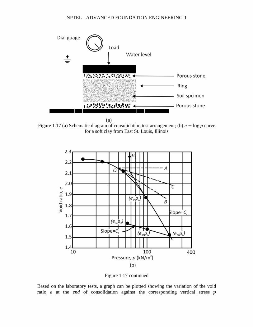
Laboratory tests on undisturbed saturated clay specimens can be conducted (ASTM Test Designation D-2435) to determine the consolidation settlement caused by various incremental loadings. The test specimens are usually 2.5 in. (63.5 mm) in diameter and 1 in. (25.4 mm) in height. Specimens are placed inside a ring, with one porous stone at the top and one at the bottom of the specimen (figure 1.17a). Load on the specimen is then applied so that the total vertical stress is equal to 𝑝𝑝. Settlement readings for the specimen are taken for 24 hours. After that, the load on the specimen is doubled and settlement readings are taken. At all times during the test the specimen is kept under water. This procedure is continued until the desired limit of stress on the clay specimen is reached.


Figure 1.17 (a) Schematic diagram of consolidation test arrangement; (b) 𝑒𝑒 − log 𝑝𝑝 curve for a soft clay from East St. Louis, Illinois

Figure 1.17 continued

Based on the laboratory tests, a graph can be plotted showing the variation of the void ratio 𝑒𝑒 at the end of consolidation against the corresponding vertical stress 𝑝𝑝


(semilogarithmic graph: 𝑒𝑒 on the arithmetic scale and 𝑝𝑝 on the log scale). The nature of variation of 𝑒𝑒 against log 𝑝𝑝 for a clay specimen is shown in figure 1.17b. After the desired consolidation pressure has been reached, the specimen can be gradually unloaded, which will result in the swelling of the specimen. Figure 1.17b also shows the variation of the void ratio during the unloading period.

From the 𝑒𝑒 − log − 𝑝𝑝 curve shown in figure 1.17b, three parameters necessary for calculating settlement in the field can be determined.

1. The preconsolidation pressure, 𝑝𝑝𝑐𝑐 , is the maximum past effective overburden pressure to which the soil specimen has been subjected. It can be determined by using a simple graphical procedure as proposed by Casegrande (1936). This procedure for determining the preconsolidation pressure, with reference to figure 1.17b, involves five steps: a. Determine the point O on the 𝑒𝑒 − log𝑝𝑝 curve that has the sharpest curvature

(that is, the smallest radius of curvature). b. Draw a horizontal line OA. c. Draw a line OB that is tangent to the 𝑒𝑒 − log𝑝𝑝 curve at O. d. Draw a line OC that bisects the angle AOB, e. Produce the straight-line portion of the 𝑒𝑒 − log 𝑝𝑝 curve backward to intersect

OC. This is point D. the pressure that corresponds to point 𝑝𝑝 is the preconsolidation pressure, 𝑝𝑝𝑐𝑐 .

Natural soil deposits can be normally consolidated or overconsolidated (or preconsolidated). If the present effective overburden pressure 𝑝𝑝 = 𝑝𝑝𝑎𝑎 is equal to the preconsolidated pressure 𝑝𝑝𝑐𝑐 the soil is normally consolidated. However, if 𝑝𝑝𝑜𝑜 < 𝑝𝑝𝑐𝑐 , the sol is overconsolidated.

Preconsolidation pressure (𝑝𝑝𝑐𝑐) has been correlated with the index parameters by several investigators. Stas and Kulhawy (1984) suggested that

𝑝𝑝𝑐𝑐𝜎𝜎𝑎𝑎

= 10(1.11−1.62𝐿𝐿𝐿𝐿) [1.53a]

Where

𝜎𝜎𝑎𝑎 = atmospheric stress in derived unit

𝐿𝐿𝐿𝐿 = liquidity index

The liquidity index of a soil is defined as

𝐿𝐿𝐿𝐿 = 𝑤𝑤−𝑃𝑃𝐿𝐿𝐿𝐿𝐿𝐿_𝑃𝑃𝐿𝐿

[1.53b]

Where

𝑤𝑤 = 𝑖𝑖𝑖𝑖 𝑠𝑠𝑖𝑖𝑡𝑡𝑢𝑢 moisture content


𝐿𝐿𝐿𝐿 = liquid limit

𝑃𝑃𝐿𝐿 = plastic limit

Nagaraj and Murthy (1985) provided an empirical relation to calculate 𝑝𝑝𝑐𝑐 , which is as follows:

kN/m2 ↓

log 𝑝𝑝𝑐𝑐 =1.122−�𝑒𝑒𝑜𝑜𝑒𝑒𝐿𝐿

�−0.0463 log 𝑝𝑝𝑜𝑜

0.188 ↑

kN/m2

[1.54]

Where

𝑒𝑒𝑜𝑜 = 𝑖𝑖𝑖𝑖 𝑠𝑠𝑖𝑖𝑡𝑡𝑢𝑢 void ratio

𝑝𝑝𝑜𝑜 = 𝑖𝑖𝑖𝑖𝑠𝑠𝑖𝑖𝑡𝑡𝑢𝑢 effective overburden pressure

𝑒𝑒𝐿𝐿 = void ratio of the soil at liquid limit

𝑒𝑒𝐿𝐿 = �𝐿𝐿𝐿𝐿(%)100

� 𝐺𝐺𝑠𝑠 [1.55]

The U. S. Department of the Navy (1982) also provided generalized relationships between 𝑝𝑝𝑐𝑐 , 𝐿𝐿𝐿𝐿 and the sensitivity of clayey soils (𝑆𝑆𝑡𝑡). This relationship was also recommended by Kulhawy and Mayne (1990). The definition of sensitivity is given in section. Figure 1.18 shows the relationship.

Figure 1.18 Variation of 𝑝𝑝𝑐𝑐 with LI (after U. S. Department of the Navy, 1982)


2. The compression index, 𝐶𝐶𝑐𝑐 , is the slope of straight-line portion (latter part of the loading curve), or 𝐶𝐶𝑐𝑐 = 𝑒𝑒1−𝑒𝑒2

log 𝑝𝑝2−log 𝑝𝑝1= 𝑒𝑒1−𝑒𝑒2

log �𝑝𝑝2𝑝𝑝1� [1.56]

where 𝑒𝑒1and 𝑒𝑒2 are the void ratios at the end of consolidation under stresses 𝑝𝑝1and 𝑝𝑝2, respectively

The compression index, as determined from the laboratory 𝑒𝑒 − log𝑝𝑝 curve, will be somewhat different from that encountered in the field. The primary reason is that the soil remolds to some degree during the field exploration. The nature of variation of the 𝑒𝑒 − log𝑝𝑝 curve in the field for normally consolidated clay is shown in figure 1.19. It is generally referred to as the virgin compression curve. The virgin curve approximately intersects the laboratory curve at a void ratio of 0.42𝑒𝑒𝑜𝑜 (Terzaghi and Peck, 1967). Note that 𝑒𝑒𝑜𝑜 is the void ratio of the clay in the field. Knowing the values of 𝑒𝑒𝑜𝑜 and 𝑝𝑝𝑐𝑐 you can easily construct the virgin curve and calculate the compression index of the virgin curve by using equation (56).

Figure 1.19 Construction of virgin compression curve for normally consolidated clay


The value of 𝐶𝐶𝑐𝑐 can vary widely depending on the soil. Skempton (1944) has given am empirical correlation for the compression index in which

𝐶𝐶𝑐𝑐 = 0.009(𝐿𝐿𝐿𝐿 − 10) [1.57]

Where


Besides Skempton, other investigators have proposed correlations for the compression index. Some of these correlations are summarized in table 14.

3. The swelling index, 𝐶𝐶𝑠𝑠, is the slope of the unloading portion of the 𝑒𝑒 − log𝑝𝑝 curve. In figure 1.17b, it can be defined as 𝐶𝐶𝑠𝑠 = 𝑒𝑒3−𝑒𝑒4

log �𝑝𝑝4𝑝𝑝3� [1.58]

In most cases the value of the swelling index (𝐶𝐶𝑠𝑠) is 14 to 1

5 of the compression index. Flowing are some representative values of 𝐶𝐶𝑠𝑠/𝐶𝐶𝑐𝑐 for natural soil deposits. The swelling index is also referred to as the recompression index.

Description of soil 𝐶𝐶𝑠𝑠/𝐶𝐶𝑐𝑐

Boston Blue clay 0.24-0.33

Chicago clay 0.15-0.3

New Orleans clay 0.15-0.28

St. Lawrence clay 0.05-0.1

Table 14 Correlations for Compression Index

Reference Correlation

Azzouz, Krizek, and Corotis (1976) 𝐶𝐶𝑐𝑐 = 0.01 𝑤𝑤𝑖𝑖 (Chicago clay)

𝐶𝐶𝑐𝑐 = 0.208 𝑒𝑒𝑜𝑜 + 0.0083 (Chicago clay)

𝐶𝐶𝑐𝑐 = 0.0115 𝑤𝑤𝑖𝑖 (organic soils, peat)

𝐶𝐶𝑐𝑐 = 0.0046(𝐿𝐿𝐿𝐿 − 9) (Brazillian clay)


Rendon-Herrero (1980) 𝐶𝐶𝑐𝑐 = 0.141𝐺𝐺𝑠𝑠12 �

1 + 𝑒𝑒𝑜𝑜𝐺𝐺𝑠𝑠

�2.38

Nagaraj and Murthy (1985) 𝐶𝐶𝑐𝑐 = 0.2343 �𝐿𝐿𝐿𝐿

100�

𝐺𝐺𝑠𝑠

Wroth and Wood (1978) 𝐶𝐶𝑐𝑐 = 0.5𝐺𝐺𝑠𝑠 �𝑃𝑃𝐿𝐿

100�

Leroueil, Tavenas, and LeBihan (1983)

Note: 𝐺𝐺𝑠𝑠 = specific gravity of soil solids


𝑃𝑃𝐿𝐿 = plasticity index

𝑆𝑆𝑡𝑡 = sensitivity

𝑤𝑤𝑖𝑖 = natural moisture content

The swelling index determination is important in the estimation of consolidation settlement of overconsolidated clays. In the field, depending on the pressure increase, an overconsolidated clay will follow an e-log 𝑝𝑝 path 𝑎𝑎𝑎𝑎𝑐𝑐, as shown in figure 1.20. Note that point 𝑎𝑎 with coordinates of 𝑝𝑝𝑜𝑜 and 𝑒𝑒𝑜𝑜 corresponds to the field condition before any pressure increase. Point 𝑎𝑎 corresponds to the preconsolidation pressure (𝑝𝑝𝑐𝑐) of the clay. Line 𝑎𝑎𝑎𝑎 is approximately parallel to the laboratory unloading cure 𝑐𝑐𝑐𝑐 (Schmertmann, 1953). Hence, if you know 𝑒𝑒𝑜𝑜 ,𝑝𝑝𝑜𝑜 ,𝑝𝑝𝑐𝑐 ,𝐶𝐶𝑐𝑐 , and 𝐶𝐶𝑠𝑠, you can easily construct the field consolidation curve.


Figure 1.20 Construction of field consolidation curve for over consolidated clay

Nagaraj and Murthy (1985) expressed the swelling index as

𝐶𝐶𝑠𝑠 = 0.0463 � 𝐿𝐿𝐿𝐿100� 𝐺𝐺𝑠𝑠 [1.59]

It is essential to point out that any of the empirical correlations for 𝐶𝐶𝑐𝑐 and 𝐶𝐶𝑠𝑠 given in the section are only approximate. It may be valid for a given soil for which the relationship was developed but may not hold good for other soils. As an example, figure 1.21 shows the plots of 𝐶𝐶𝑐𝑐 and 𝐶𝐶𝑠𝑠 with liquid limit for soils from Richmond, Virginia (Martin et al., 1985). For these soils,


Figure 1.21 Variation of 𝐶𝐶𝑐𝑐 and 𝐶𝐶𝑠𝑠 with liquid limit for soils from Richmond, Virginia (after Martin et al., 1995)

𝐶𝐶𝑐𝑐 = 0.0326(𝐿𝐿𝐿𝐿 − 43.4) [1.60]

And

𝐶𝐶𝑠𝑠 = 0.00045(𝐿𝐿𝐿𝐿 + 11.9) [1.61]

The 𝐶𝐶𝑠𝑠 / 𝐶𝐶𝑐𝑐 ratio is about 125; whereas, the typical range is about1

5 to 110.

CONSOLIDATION SETTLEMENT CALCULATION

The one-dimensional consolidation settlement (caused by an additional load) of a clay layer (figure 1.22a) having a thickness 𝐻𝐻𝑐𝑐 may be calculated as


𝑆𝑆 = Δ𝑒𝑒1+𝑒𝑒𝑜𝑜

𝐻𝐻𝑐𝑐 [1.62]

Figure 1.22 One-dimensional settlement calculation: (b) is for equation (64); (c) is for equations (66 and 68)

Where

𝑆𝑆 = settlement

Δ𝑒𝑒 = total change of void ratio caused by the additional load application

𝑒𝑒𝑜𝑜 = the void ratio of the clay before the application of load

Note that

Δ𝑒𝑒1+𝑒𝑒𝑜𝑜

= 𝜀𝜀𝑣𝑣 = vertical strain

For normally consolidated clay, the field 𝑒𝑒 − log 𝑝𝑝 curve will be like the one shown in figure 1.22b. If 𝑝𝑝𝑜𝑜 = initial average effective overburden pressure on the clay layer and Δ𝑝𝑝 = average pressure increase on the clay layer caused by the added load, the change of void ratio caused by the load increase is


Δ𝑒𝑒 = 𝐶𝐶𝑐𝑐 log 𝑝𝑝𝑜𝑜+Δ𝑝𝑝𝑝𝑝𝑜𝑜

[1.63]

Now, combining equations (62 and 63) yields

𝑆𝑆 = 𝐶𝐶𝑐𝑐𝐻𝐻𝑐𝑐1+𝑒𝑒𝑜𝑜

log 𝑝𝑝𝑜𝑜+Δ𝑝𝑝𝑝𝑝𝑜𝑜

[1.64]

For overconsolidated clay, the field 𝑒𝑒 − log𝑝𝑝 curve will be like the one show figure 1.22c. In this case, depending on the value of Δ𝑝𝑝, two conditions may at. First, if 𝑝𝑝𝑜𝑜 + Δ𝑝𝑝 < 𝑝𝑝𝑐𝑐 ,

Δ𝑒𝑒 = 𝐶𝐶𝑠𝑠 log 𝑝𝑝𝑜𝑜+Δ𝑝𝑝𝑝𝑝𝑜𝑜

[1.65]

Combining equations (62 and 65) gives

𝑆𝑆 = 𝐻𝐻𝑐𝑐𝐶𝐶𝑠𝑠1+𝑒𝑒𝑜𝑜

log 𝑝𝑝𝑜𝑜+Δ𝑝𝑝𝑝𝑝𝑜𝑜

[1.66]

Second, if 𝑝𝑝𝑜𝑜 < 𝑝𝑝𝑐𝑐 < 𝑝𝑝𝑜𝑜 + ∆𝑝𝑝,

∆𝑒𝑒 = ∆𝑒𝑒1 + ∆𝑒𝑒2 = 𝐶𝐶𝑧𝑧 log 𝑝𝑝𝑐𝑐𝑝𝑝𝑜𝑜

+ 𝐶𝐶𝑐𝑐 log 𝑝𝑝𝑜𝑜+Δ𝑝𝑝𝑝𝑝𝑜𝑜

[1.67]

Now, combining equations (62 and 67) yields

𝑆𝑆 = 𝐶𝐶𝑠𝑠𝐻𝐻𝑐𝑐1+𝑒𝑒𝑜𝑜

log 𝑝𝑝𝑐𝑐𝑝𝑝𝑜𝑜

+ 𝐶𝐶𝑐𝑐𝐻𝐻𝑐𝑐1+𝑒𝑒𝑜𝑜

log 𝑝𝑝𝑜𝑜+Δ𝑝𝑝𝑝𝑝𝑐𝑐

[1.68]

TIME RATE OF CONSOLIDATION

In section we showed that consolidation is the result gradual dissipation of the excess pore water pressure from a clay layer. Pore water pressure dissipation, in turn, increases the effective stress, which induces settlement. Hence, to estimate the degree of consolidation of a clay layer at some time t after the load application, you need to know the rate of dissipation of the excess pore water pressure.

Figure 1.23 shows a clay layer of thickness 𝐻𝐻𝑐𝑐 that has highly permeable sand layers at its top and bottom. Here, the excess pore pressure at any point at any time t after the load application is ∆𝑢𝑢 = (∆ℎ)𝛾𝛾𝑤𝑤 . For a vertical drainage condition (that is, in the direction of z only) from the clay layer, Terzaghi derived the following differential equation:


Figure 1.23 (a) Derivation of equation (71); (b) nature of variation of ∆𝑢𝑢 with time

𝜕𝜕(∆𝑢𝑢)𝜕𝜕𝑡𝑡

= 𝐶𝐶𝑣𝑣𝜕𝜕2(∆𝑢𝑢)𝜕𝜕𝑧𝑧 2 [1.69]

Where

𝐶𝐶𝑣𝑣 = coefficient of consolidation

𝐶𝐶𝑣𝑣 = 𝑘𝑘𝑚𝑚𝑣𝑣𝛾𝛾𝑤𝑤

= 𝑘𝑘∆𝑒𝑒

∆𝑝𝑝 (1+𝑒𝑒𝑎𝑎𝑣𝑣 )𝛾𝛾𝑤𝑤 [1.70]

Where

𝑘𝑘 = hydraulic conductivity of the clay

∆𝑒𝑒 = total change of void ratio caused by a stress increase of ∆p

𝑒𝑒𝑎𝑎𝑣𝑣 = average void ratio during consolidation

𝑚𝑚𝑣𝑣 = volume coefficient of compressibility = ∆𝑒𝑒/[∆𝑝𝑝(1 + 𝑒𝑒𝑎𝑎𝑣𝑣)]

Equation (69) can be solved to obtain ∆𝑢𝑢 as a function of time t with the following boundary conditions:


1. Because highly permeable sand layers are located at 𝑧𝑧 = 0 and 𝑧𝑧 = 𝐻𝐻𝑐𝑐 , the excess pore water pressure developed in the clay at those points will be immediately dissipated. Hence ∆𝑢𝑢 = 0 at 𝑧𝑧 = 0 ∆𝑢𝑢 = 0 at 𝑧𝑧 = 𝐻𝐻𝑐𝑐 = 2𝐻𝐻 Where 𝐻𝐻 = Length of maximum drainage path (due to two-way drainage condition-that is, at the top and bottom of the clay)

2. At time 𝑡𝑡 = 0, ∆𝑢𝑢 = ∆𝑢𝑢𝑜𝑜 = initial excess pore water pressure after the load application With the preceding boundary conditions, equation (69) yields ∆𝑢𝑢 = ∑ �2(∆𝑢𝑢𝑜𝑜 )

𝑀𝑀𝑠𝑠𝑖𝑖𝑖𝑖 �𝑀𝑀𝑧𝑧

𝐻𝐻�� 𝑒𝑒−𝑀𝑀2𝑇𝑇𝑣𝑣𝑚𝑚=∞

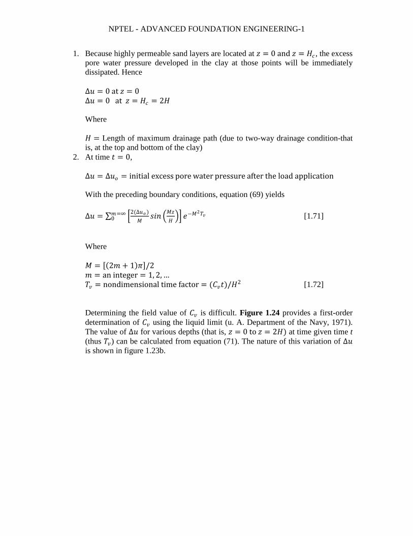
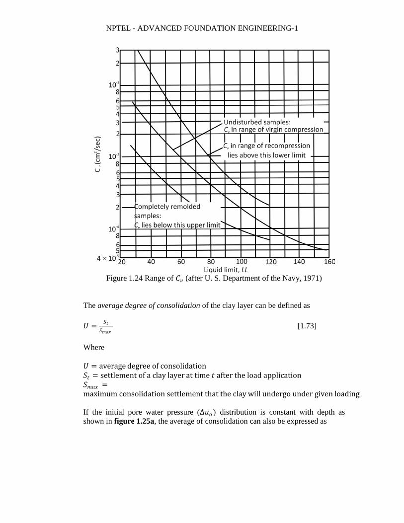
0 [1.71] Where 𝑀𝑀 = [(2𝑚𝑚 + 1)𝜋𝜋]/2 𝑚𝑚 = an integer = 1, 2, … 𝑇𝑇𝑣𝑣 = nondimensional time factor = (𝐶𝐶𝑣𝑣𝑡𝑡)/𝐻𝐻2 [1.72] Determining the field value of 𝐶𝐶𝑣𝑣 is difficult. Figure 1.24 provides a first-order determination of 𝐶𝐶𝑣𝑣 using the liquid limit (u. A. Department of the Navy, 1971). The value of ∆𝑢𝑢 for various depths (that is, 𝑧𝑧 = 0 to 𝑧𝑧 = 2𝐻𝐻) at time given time t (thus 𝑇𝑇𝑣𝑣) can be calculated from equation (71). The nature of this variation of ∆𝑢𝑢 is shown in figure 1.23b.


Figure 1.24 Range of 𝐶𝐶𝑣𝑣 (after U. S. Department of the Navy, 1971)

The average degree of consolidation of the clay layer can be defined as 𝑈𝑈 = 𝑆𝑆𝑡𝑡

𝑆𝑆𝑚𝑚𝑎𝑎𝑚𝑚 [1.73]

Where 𝑈𝑈 = average degree of consolidation 𝑆𝑆𝑡𝑡 = settlement of a clay layer at time 𝑡𝑡 after the load application 𝑆𝑆𝑚𝑚𝑎𝑎𝑚𝑚 =maximum consolidation settlement that the clay will undergo under given loading If the initial pore water pressure (∆𝑢𝑢𝑜𝑜) distribution is constant with depth as shown in figure 1.25a, the average of consolidation can also be expressed as


Figure 1.25 Drainage condition for consolidation: (a) two-way drainage; (b) one-

way drainage

𝑈𝑈 = 𝑆𝑆𝑡𝑡𝑆𝑆𝑚𝑚𝑎𝑎𝑚𝑚

= ∫ (∆𝑢𝑢𝑜𝑜 )𝑐𝑐𝑧𝑧−∫ (∆𝑢𝑢)𝑐𝑐𝑧𝑧2𝐻𝐻0

2𝐻𝐻0

∫ (∆𝑢𝑢𝑜𝑜 )𝑐𝑐𝑧𝑧 2𝐻𝐻0

[1.74] Or

𝑈𝑈 =(∆𝑢𝑢𝑜𝑜 )2𝐻𝐻−∫ (∆𝑢𝑢)𝑐𝑐𝑧𝑧2𝐻𝐻

0(∆𝑢𝑢𝑜𝑜 )2𝐻𝐻

= 1 − ∫ (∆𝑢𝑢)𝑐𝑐𝑧𝑧2𝐻𝐻02𝐻𝐻(∆𝑢𝑢𝑜𝑜 )

[1.75] Now, combining equations (71 and 75) we obtain 𝑈𝑈 = 𝑆𝑆𝑡𝑡

𝑆𝑆𝑚𝑚𝑎𝑎𝑚𝑚= 1 − ∑ � 2

𝑀𝑀2� 𝑒𝑒−𝑀𝑀2𝑇𝑇𝑣𝑣𝑚𝑚=∞

𝑚𝑚=0 [1.76] The variation of 𝑈𝑈 with 𝑇𝑇𝑣𝑣 can be calculated from equation (76) and is plotted in figure 1.26. Note that equation (76) and thus figure 1.26 are also valid when an impermeable layer is located at the bottom of the clay layer (figure 1.25b). In that case, excess pore water pressure dissipation can take place in one direction only.


Figure 1.26 Plot of time factor against average degree of consolidation (∆𝑢𝑢𝑜𝑜 =constant)

The length of the maximum drainage path then is equal to 𝐻𝐻 = 𝐻𝐻𝑐𝑐 .

The variation of 𝑇𝑇𝑣𝑣 with 𝑈𝑈 shown in figure 1.26 can also be approximated by

𝑇𝑇𝑣𝑣 = 𝜋𝜋4�𝑈𝑈%

100�

2 (for 𝑈𝑈 = 0 − 60%) [1.77]

And

𝑇𝑇𝑣𝑣 = 1.781 − 0.933 log(100 − 𝑈𝑈%) (for 𝑈𝑈 > 60%) [1.78]

Sivaram and Swamee (1977) have also developed an empirical relationship between 𝑇𝑇𝑣𝑣 and 𝑈𝑈 that is valid for U varying from 0 to 100%. It is of the form

𝑇𝑇𝑣𝑣 =�𝜋𝜋4�

𝑈𝑈%100�

2�

�1−�𝑈𝑈%100�

5.6�

0.357 [1.79]

In some cases, initial excess pore water pressure may not be constant with depth as shown in figure 1.25. Following are a few cases of those and the solutions for the average degree of consolidation.


Trapezoidal Variation Figure 1.27 shows a trapezoidal variation of initial excess pore water pressure with two-way drainage. For this case the variation of 𝑇𝑇𝑣𝑣 with 𝑈𝑈 will be the same as shown in figure 1.26.

Figure 1.27 Trapezoidal initial excess pore water pressure distribution

Sinusoidal Variation This variation is shown in figures 1.28a and 1.28b. For the initial excess pore water pressure variation shown in figure 1.28a,

z

Figure 1.28 Sinusoidal initial excess pore water pressure distribution


∆𝑢𝑢 = ∆𝑢𝑢𝑜𝑜𝑠𝑠𝑖𝑖𝑖𝑖𝜋𝜋𝑧𝑧2𝐻𝐻

[1.80]

Similarly, for the case shown in figure 1.28b,

∆𝑢𝑢 = ∆𝑢𝑢𝑜𝑜𝑐𝑐𝑜𝑜𝑠𝑠𝜋𝜋𝑧𝑧4𝐻𝐻

[1.81]

The variations of 𝑇𝑇𝑣𝑣 with 𝑈𝑈 for these two cases are shown in figure 1.29

Figure 1.29 Variation of 𝑈𝑈 with 𝑇𝑇𝑣𝑣 − sinusoidal variation of initial excess pore water pressure distribution

Triangular Variation Figures 1.30 and 1.31 show several types of initial pore water pressure variation and the variation of 𝑇𝑇𝑣𝑣 with the average degree of consolidation.


z

Figure 1.30 Variation of 𝑈𝑈 with 𝑇𝑇𝑣𝑣 − triangular initial excess pore water pressure distribution

Figure 1.31 triangular initial excess pore water pressure distribution-variation of 𝑈𝑈 with 𝑇𝑇𝑣𝑣


Example 9

A laboratory consolidation test on normally consolidated clay showed the following

Load, 𝑝𝑝(kN/m2) Void ratio at the end of consolidation, e

140 0.92

212 0.86

The specimen tested was 25.4 mm in thickness and drained on both sides. The time required for the specimen to reach 50% consolidation was 4.5 min.

A similar clay layer in the field, 2.8 m thick and drained on both sides, is subjected to similar average pressure increase (that is, 𝑝𝑝𝑜𝑜 = 140 kN/m2 and po + ∆p = 212kN/m2). Determine the

a. Expected maximum consolidation settlement in the field b. Length of time required for the total settlement in the field to reach 40 mm

(assume uniform initial excess pore water pressure increase with depth)

Solution

Part a

For normally consolidated clay [equation 56]

𝐶𝐶𝑐𝑐 = 𝑒𝑒1−𝑒𝑒2

𝑙𝑙𝑜𝑜𝑙𝑙 �𝑝𝑝2𝑝𝑝1�

= 0.92−0.86

𝑙𝑙𝑜𝑜𝑙𝑙�212140�

= 0.333

From equation (64)

𝑆𝑆 = 𝐶𝐶𝑐𝑐𝐻𝐻𝑐𝑐1+𝑒𝑒𝑜𝑜

𝑙𝑙𝑜𝑜𝑙𝑙 𝑝𝑝𝑜𝑜+∆𝑝𝑝𝑝𝑝𝑜𝑜

= (0.333)(2.8)1+0.92

𝑙𝑙𝑜𝑜𝑙𝑙 212140

= 0.0875 m = 87.5 mm

Part b

From equation (73) the average degree of consolidation is

𝑈𝑈 = 𝑆𝑆𝑡𝑡𝑆𝑆𝑚𝑚𝑎𝑎𝑚𝑚

= 4087.5

(100) = 45.7%

The coefficient of consolidation, 𝐶𝐶𝑣𝑣, can be calculated from the laboratory test.

From equation (72)

𝑇𝑇𝑣𝑣 = 𝐶𝐶𝑣𝑣𝑡𝑡𝐻𝐻2


For 50% consolidation (figure 1.26), 𝑇𝑇𝑣𝑣 = 0.197, 𝑡𝑡 = 4.5 min, and 𝐻𝐻 = 𝐻𝐻𝑐𝑐/2 =12.7 mm, so

𝐶𝐶𝑣𝑣 = 𝑇𝑇50𝐻𝐻2

𝑡𝑡= (0.197)(12.7)2

4.5= 7.061 mm2/min

Again, for field consolidation, 𝑈𝑈 = 45.7%. From equation (77)

𝑇𝑇𝑣𝑣 = 𝜋𝜋4�𝑈𝑈%

100�

2= 𝜋𝜋

4�45.7

100�

2= 0.164

But

𝑇𝑇𝑣𝑣 = 𝐶𝐶𝑣𝑣𝑡𝑡𝐻𝐻2

Or

𝑡𝑡 = 𝑇𝑇𝑣𝑣𝐻𝐻2

𝐶𝐶𝑣𝑣=

0.164�2.8×10002 �

2

7.061= 45,523 min = 31.6 days

module 1 (lecture 3) geotechnical properties of soil and...

Documents