models used in asset dynamics
TRANSCRIPT
Lecture 11 Models of asset dynamics
Reading: Luenberger Chapter 11
True multiperiod investments fluctuate in value, pay out random dividends, exist
in an environment of variable interest rates, and are subject to a continuing
variety of other uncertainties.
No investment principles in this chapter. Introduce mathematical models that
form the foundation for analyses developed later. The goal is to develop the
mathematical framework by means of which we can generate realistic stock
price movement.
Primary model types used to represent asset dynamics:
• Binomial lattices are widely applicable. Many real investment
problems can be formulated and solved using the binomial lattice
framework. Textbook: 80% of the materials in later chapters are
presented in terms of binomial models.
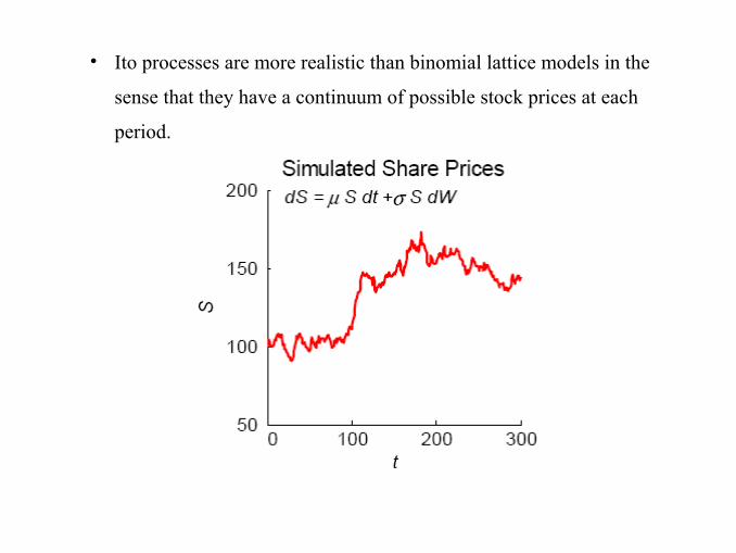
• Ito processes are more realistic than binomial lattice models in the
sense that they have a continuum of possible stock prices at each
period.
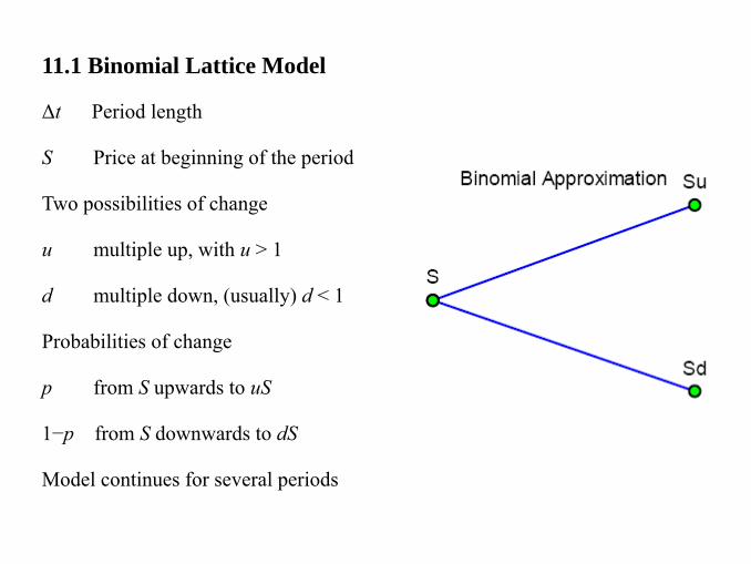
11.1 Binomial Lattice Model
Δt Period length
S Price at beginning of the period
Two possibilities of change
u multiple up, with u > 1
d multiple down, (usually) d < 1
Probabilities of change
p from S upwards to uS
1−p from S downwards to dS
Model continues for several periods
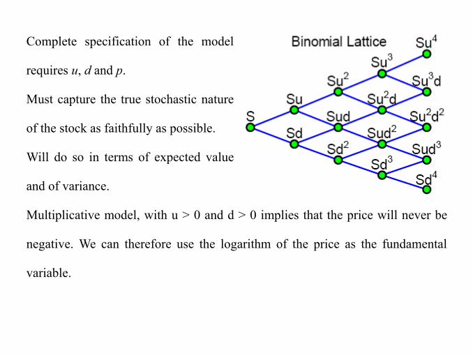
Complete specification of the model
requires u, d and p.
Must capture the true stochastic nature
of the stock as faithfully as possible.
Will do so in terms of expected value
and of variance.
Multiplicative model, with u > 0 and d > 0 implies that the price will never be
negative. We can therefore use the logarithm of the price as the fundamental
variable.
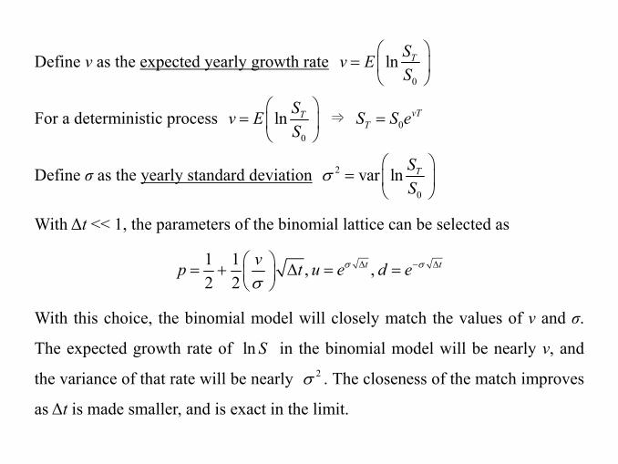
Define ν as the expected yearly growth rate 0
ln TSv ES
⎛ ⎞= ⎜ ⎟
⎝ ⎠
For a deterministic process 0
ln TSv ES
⎛ ⎞= ⎜ ⎟
⎝ ⎠ ⇒ 0
vTTS S e=
Define σ as the yearly standard deviation 2
0
var ln TSS
σ⎛ ⎞
= ⎜ ⎟⎝ ⎠
With Δt << 1, the parameters of the binomial lattice can be selected as
1 1 , ,2 2
t tvp t u e d eσ σ
σΔ − Δ⎛ ⎞= + Δ = =⎜ ⎟
⎝ ⎠
With this choice, the binomial model will closely match the values of ν and σ.
The expected growth rate of ln S in the binomial model will be nearly ν, and
the variance of that rate will be nearly 2σ . The closeness of the match improves
as Δt is made smaller, and is exact in the limit.
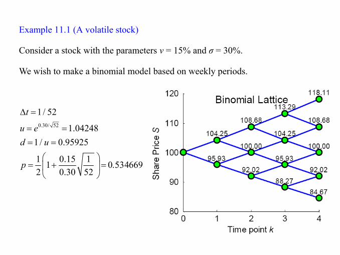
Example 11.1 (A volatile stock)
Consider a stock with the parameters ν = 15% and σ = 30%.
We wish to make a binomial model based on weekly periods.
0.30/ 52
1 / 52
1.042481 / 0.95925
1 0.15 112 0.30 52
t
u ed u
p
Δ =
= == =
⎛ ⎞= + = 0.534669 ⎜ ⎟
⎝ ⎠
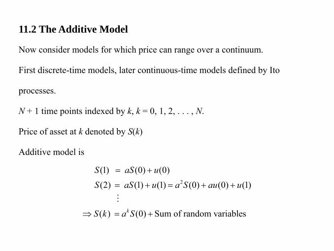
11.2 The Additive Model
Now consider models for which price can range over a continuum.
First discrete-time models, later continuous-time models defined by Ito
processes.
N + 1 time points indexed by k, k = 0, 1, 2, . . . , N.
Price of asset at k denoted by S(k)
Additive model is
2
(1) (0) (0)(2) (1) (1) (0) (0) (1)
( ) (0) Sum of random variablesk
S aS uS aS u a S au u
S k a S
= +
= + = + +
⇒ = +
M
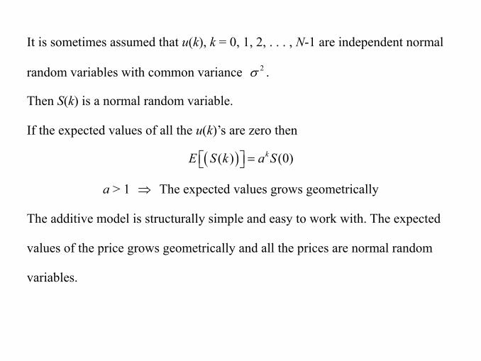
It is sometimes assumed that u(k), k = 0, 1, 2, . . . , N-1 are independent normal
random variables with common variance 2σ .
Then S(k) is a normal random variable.
If the expected values of all the u(k)’s are zero then
( )( ) (0)kE S k a S=⎡ ⎤⎣ ⎦
a > 1 ⇒ The expected values grows geometrically
The additive model is structurally simple and easy to work with. The expected
values of the price grows geometrically and all the prices are normal random
variables.
Model is seriously flawed because it lacks realism:
• Normal random variables can be negative ⇒ prices might be negative
• Standard deviation should increase as the price increases
Now consider the multiplicative model, where we will use our understanding of
the additive model.
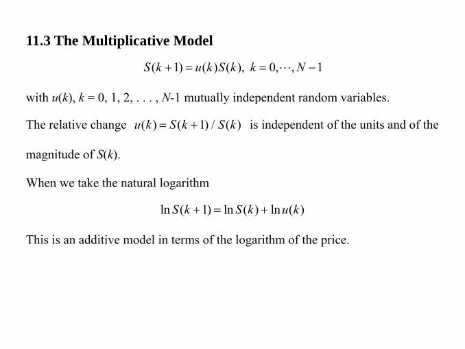
11.3 The Multiplicative Model
( 1) ( ) ( ), 0, , 1S k u k S k k N+ = = −L
with u(k), k = 0, 1, 2, . . . , N-1 mutually independent random variables.
The relative change ( ) ( 1) / ( )u k S k S k= + is independent of the units and of the
magnitude of S(k).
When we take the natural logarithm
ln ( 1) ln ( ) ln ( )S k S k u k+ = +
This is an additive model in terms of the logarithm of the price.
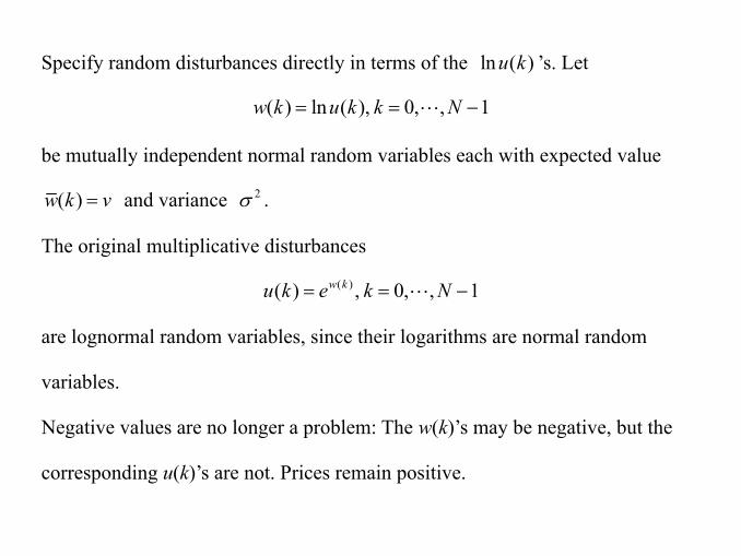
Specify random disturbances directly in terms of the ln ( )u k ’s. Let
( ) ln ( ), 0, , 1w k u k k N= = −L
be mutually independent normal random variables each with expected value
( )w k v= and variance 2σ .
The original multiplicative disturbances
( )( ) , 0, , 1w ku k e k N= = −L
are lognormal random variables, since their logarithms are normal random
variables.
Negative values are no longer a problem: The w(k)’s may be negative, but the
corresponding u(k)’s are not. Prices remain positive.
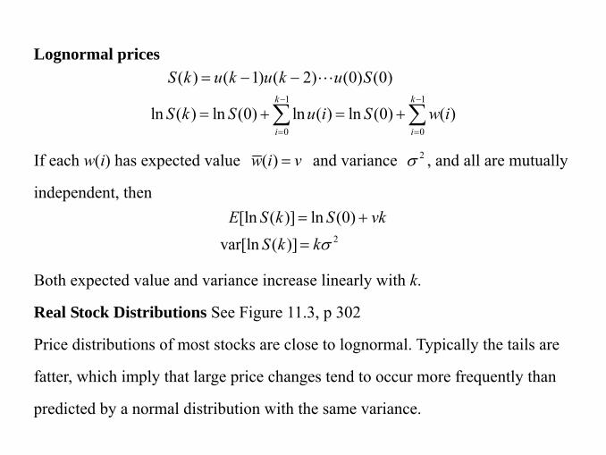
Lognormal prices
1 1
0 0
( ) ( 1) ( 2) (0) (0)
ln ( ) ln (0) ln ( ) ln (0) ( )k k
i i
S k u k u k u S
S k S u i S w i− −
= =
= − −
= + = +∑ ∑
L
If each w(i) has expected value ( )w i v= and variance 2σ , and all are mutually
independent, then
2
[ln ( )] ln (0)var[ln ( )]
E S k S vkS k kσ
= +
=
Both expected value and variance increase linearly with k.
Real Stock Distributions See Figure 11.3, p 302
Price distributions of most stocks are close to lognormal. Typically the tails are
fatter, which imply that large price changes tend to occur more frequently than
predicted by a normal distribution with the same variance.
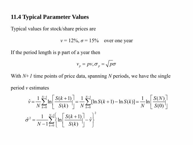
11.4 Typical Parameter Values
Typical values for stock/share prices are
ν = 12%, σ = 15% over one year
If the period length is p part of a year then
,p pv pv pσ σ= =
With N+1 time points of price data, spanning N periods, we have the single
period v estimates 1 1
0 0
21
2
0
1 ( 1) 1 1 ( )ˆ ln [ln ( 1) ln ( )] ln( ) (0)
1 ( 1)ˆ ˆln1 ( )
N N
k k
N
k
S k S Nv S k S kN S k N N S
S k vN S k
σ
− −
= =
−
=
⎡ ⎤ ⎡ ⎤+ = = + − =⎢ ⎥ ⎢ ⎥
⎣ ⎦ ⎣ ⎦
⎧ ⎫⎡ ⎤+= −⎨ ⎬⎢ ⎥− ⎣ ⎦⎩ ⎭
∑ ∑
∑
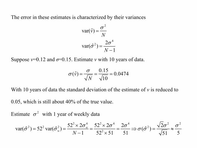
The error in these estimates is characterized by their variances 2
42
ˆvar( )
2ˆvar( )1
vN
N
σ
σσ
=
=−
Suppose ν=0.12 and σ=0.15. Estimate ν with 10 years of data.
0.15ˆ( ) 0.047410
vN
σσ = = =
With 10 years of data the standard deviation of the estimate of ν is reduced to
0.05, which is still about 40% of the true value.
Estimate 2σ with 1 year of weekly data 2 4 2 4 4 2 2
2 2 2 22
52 2 52 2 2 2ˆ ˆ ˆvar( ) 52 var( ) ( )1 52 51 51 551
ww N
σ σ σ σ σσ σ σ σ× ×= = = = ⇒ = ≈
− ×
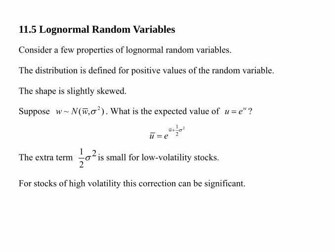
11.5 Lognormal Random Variables
Consider a few properties of lognormal random variables.
The distribution is defined for positive values of the random variable.
The shape is slightly skewed.
Suppose 2~ ( , )w N w σ . What is the expected value of wu e= ?
212
wu e
σ+=
The extra term 1 22
σ is small for low-volatility stocks.
For stocks of high volatility this correction can be significant.
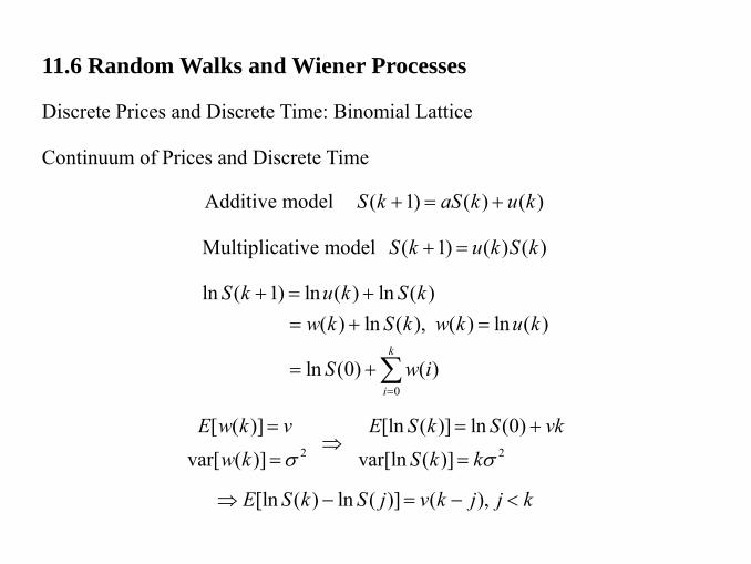
11.6 Random Walks and Wiener Processes
Discrete Prices and Discrete Time: Binomial Lattice
Continuum of Prices and Discrete Time
Additive model ( 1) ( ) ( )S k aS k u k+ = +
Multiplicative model ( 1) ( ) ( )S k u k S k+ =
0
ln ( 1) ln ( ) ln ( )( ) ln ( ), ( ) ln ( )
ln (0) ( )k
i
S k u k S kw k S k w k u k
S w i=
+ = + = + =
= + ∑
2
[ ( )]var[ ( )]
E w k vw k σ
=
= ⇒ 2
[ln ( )] ln (0)var[ln ( )]
E S k S vkS k kσ
= +
=
[ln ( ) ln ( )] ( ),E S k S j v k j j k⇒ − = − <
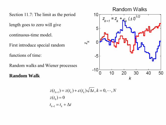
Section 11.7: The limit as the period
length goes to zero will give
continuous-time model.
First introduce special random
functions of time:
Random walks and Wiener processes
Random Walk
1
0
1
( ) ( ) ( ) , 0, ,( ) 0
k k k
k k
z t z t t t k Nz tt t t
ε+
+
= + Δ ==
= + Δ
L
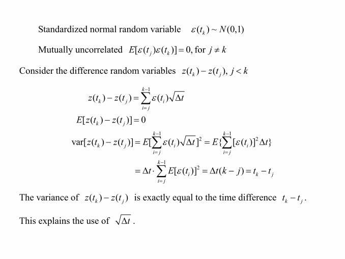
Standardized normal random variable ( ) ~ (0,1)kt Nε
Mutually uncorrelated [ ( ) ( )] 0, forj kE t t j kε ε = ≠
Consider the difference random variables ( ) ( ),k jz t z t j k− <
1
1 12 2
12
( ) ( ) ( )
[ ( ) ( )] 0
var[ ( ) ( )] [ ( ) ] { [ ( )] }
[ ( )] ( )
k
k j ii j
k j
k k
k j i ii j i j
k
i k ji j
z t z t t t
E z t z t
z t z t E t t E t t
t E t t k j t t
ε
ε ε
ε
−
=
− −
= =
−
=
− = Δ
− =
− = Δ = Δ
= Δ ⋅ = Δ − = −
∑
∑ ∑
∑
The variance of ( ) ( )k jz t z t− is exactly equal to the time difference k jt t− .
This explains the use of tΔ .
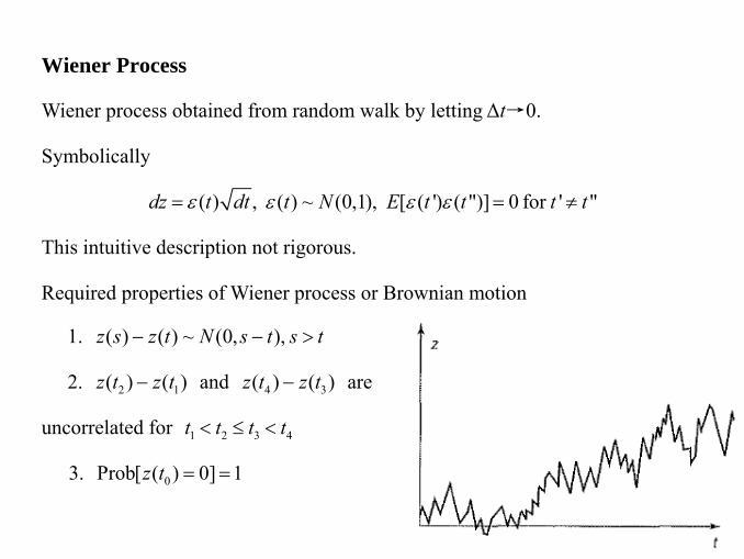
Wiener Process
Wiener process obtained from random walk by letting Δt→0.
Symbolically
( ) , ( ) ~ (0,1), [ ( ') ( ")] 0 for ' "dz t dt t N E t t t tε ε ε ε= = ≠
This intuitive description not rigorous.
Required properties of Wiener process or Brownian motion
1. ( ) ( ) ~ (0, ),z s z t N s t s t− − >
2. 2 1( ) ( )z t z t− and 4 3( ) ( )z t z t− are
uncorrelated for 1 2 3 4t t t t< ≤ <
3. 0Prob[ ( ) 0] 1z t = =
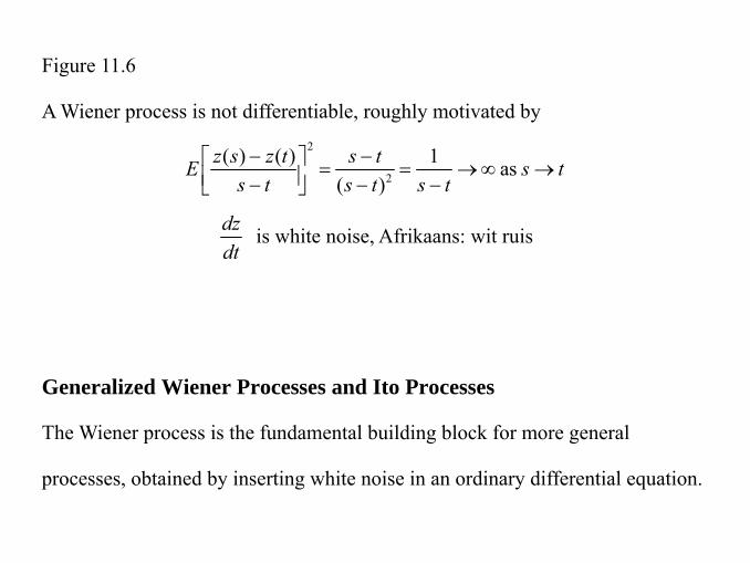
Figure 11.6
A Wiener process is not differentiable, roughly motivated by 2
2
( ) ( ) 1 as( )
z s z t s tE s ts t s t s t
− −⎡ ⎤ = = → ∞ →⎢ ⎥− − −⎣ ⎦
dzdt
is white noise, Afrikaans: wit ruis
Generalized Wiener Processes and Ito Processes
The Wiener process is the fundamental building block for more general
processes, obtained by inserting white noise in an ordinary differential equation.
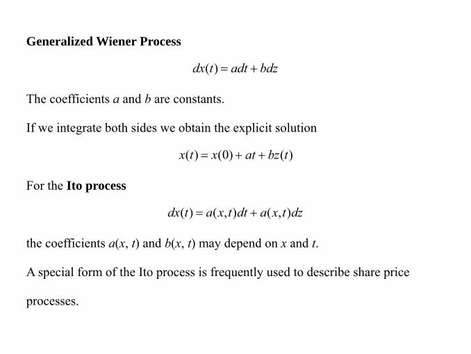
Generalized Wiener Process
( )dx t adt bdz= +
The coefficients a and b are constants.
If we integrate both sides we obtain the explicit solution
( ) (0) ( )x t x at bz t= + +
For the Ito process
( ) ( , ) ( , )dx t a x t dt a x t dz= +
the coefficients a(x, t) and b(x, t) may depend on x and t.
A special form of the Ito process is frequently used to describe share price
processes.
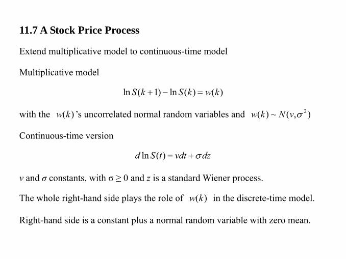
11.7 A Stock Price Process
Extend multiplicative model to continuous-time model
Multiplicative model
ln ( 1) ln ( ) ( )S k S k w k+ − =
with the ( )w k ’s uncorrelated normal random variables and 2( ) ~ ( , )w k N v σ
Continuous-time version
ln ( )d S t vdt dzσ= +
ν and σ constants, with σ ≥ 0 and z is a standard Wiener process.
The whole right-hand side plays the role of ( )w k in the discrete-time model.
Right-hand side is a constant plus a normal random variable with zero mean.
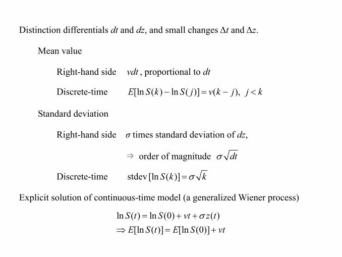
Distinction differentials dt and dz, and small changes Δt and Δz.
Mean value
Right-hand side vdt , proportional to dt
Discrete-time [ln ( ) ln ( )] ( ),E S k S j v k j j k− = − <
Standard deviation
Right-hand side σ times standard deviation of dz,
⇒ order of magnitude dtσ
Discrete-time stdev [ln ( )]S k kσ =
Explicit solution of continuous-time model (a generalized Wiener process)
ln ( ) ln (0) ( )[ln ( )] [ln (0)]
S t S vt z tE S t E S vt
σ= + +⇒ = +
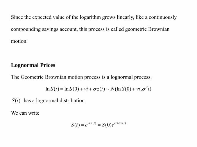
Since the expected value of the logarithm grows linearly, like a continuously
compounding savings account, this process is called geometric Brownian
motion.
Lognormal Prices
The Geometric Brownian motion process is a lognormal process.
2ln ( ) ln (0) ( ) ~ (ln (0) , )S t S vt z t N S vt tσ σ= + + +
( )S t has a lognormal distribution.
We can write
ln ( ) ( )( ) (0)S t vt z tS t e S e σ+= =
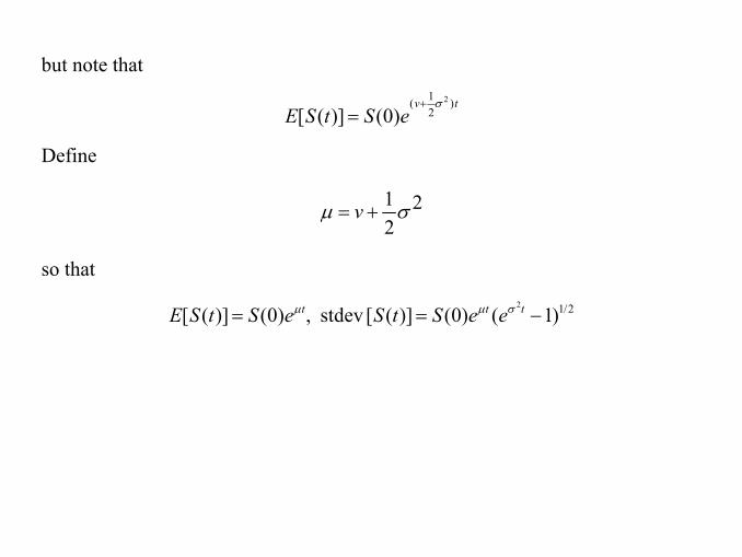
but note that 21( )
2[ ( )] (0)v t
E S t S eσ+
=
Define
1 22
vμ σ= +
so that 2 1/2[ ( )] (0) stdev [ ( )] (0) ( 1)t t tE S t S e S t S e eμ μ σ= , = −
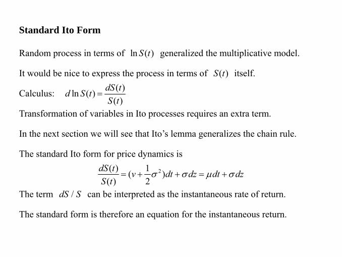
Standard Ito Form
Random process in terms of ln ( )S t generalized the multiplicative model.
It would be nice to express the process in terms of ( )S t itself.
Calculus: ( )ln ( )( )
dS td S tS t
=
Transformation of variables in Ito processes requires an extra term.
In the next section we will see that Ito’s lemma generalizes the chain rule.
The standard Ito form for price dynamics is
2( ) 1( )( ) 2
dS t v dt dz dt dzS t
σ σ μ σ= + + = +
The term /dS S can be interpreted as the instantaneous rate of return.
The standard form is therefore an equation for the instantaneous return.
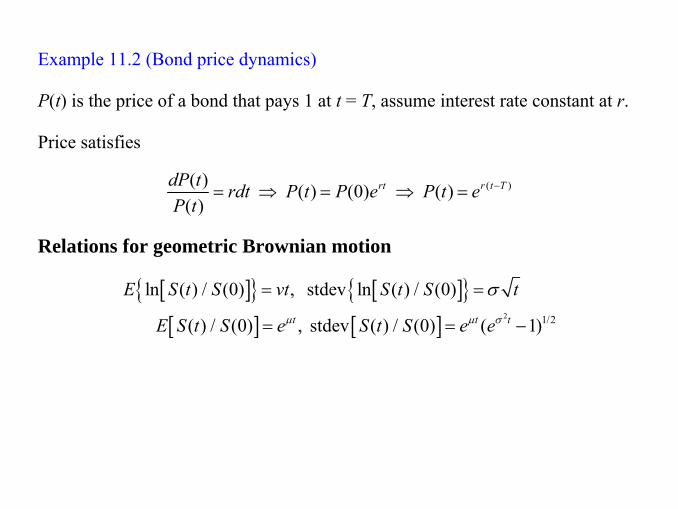
Example 11.2 (Bond price dynamics)
P(t) is the price of a bond that pays 1 at t = T, assume interest rate constant at r.
Price satisfies
( )( ) ( ) (0) ( )( )
rt r t TdP t rdt P t P e P t eP t
−= ⇒ = ⇒ =
Relations for geometric Brownian motion
[ ]{ } [ ]{ }[ ] [ ] 2 1/2
ln ( ) / (0) , stdev ln ( ) / (0)
( ) / (0) , stdev ( ) / (0) ( 1)t t t
E S t S vt S t S t
E S t S e S t S e eμ μ σ
σ= =
= = −
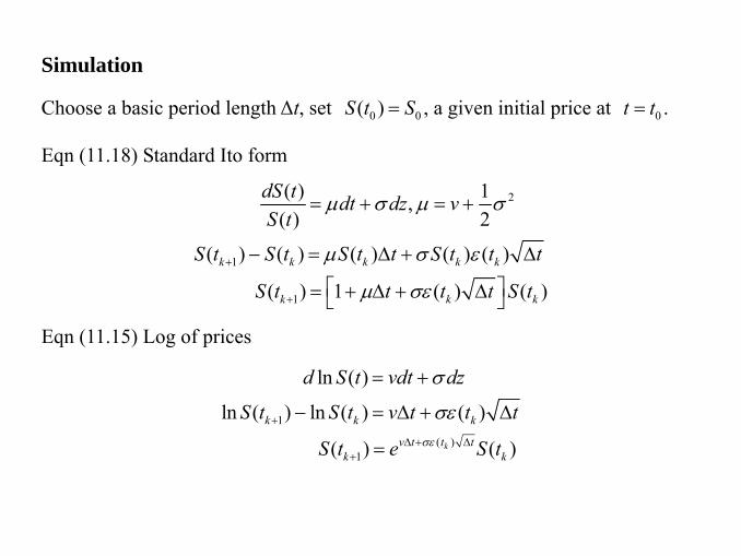
Simulation
Choose a basic period length Δt, set 0 0( )S t S= , a given initial price at 0t t= .
Eqn (11.18) Standard Ito form
2
1
1
( ) 1,( ) 2
( ) ( ) ( ) ( ) ( )
( ) 1 ( ) ( )k k k k k
k k k
dS t dt dz vS t
S t S t S t t S t t t
S t t t t S t
μ σ μ σ
μ σ ε
μ σε+
+
= + = +
− = Δ + Δ
⎡ ⎤ = + Δ + Δ⎣ ⎦
Eqn (11.15) Log of prices
1
( )1
ln ( )
ln ( ) ln ( ) ( )
( ) ( )k
k k k
v t t tk k
d S t vdt dz
S t S t v t t t
S t e S tσε
σ
σε+
Δ + Δ+
= +
− = Δ + Δ
=
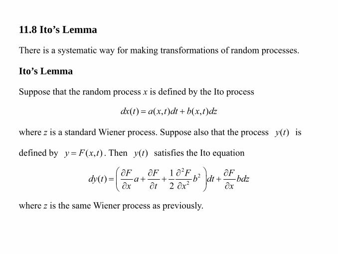
11.8 Ito’s Lemma
There is a systematic way for making transformations of random processes.
Ito’s Lemma
Suppose that the random process x is defined by the Ito process
( ) ( , ) ( , )dx t a x t dt b x t dz= +
where z is a standard Wiener process. Suppose also that the process ( )y t is
defined by ( , )y F x t= . Then ( )y t satisfies the Ito equation
22
2
1( )2
F F F Fdy t a b dt bdzx t x x
⎛ ⎞∂ ∂ ∂ ∂= + + +⎜ ⎟∂ ∂ ∂ ∂⎝ ⎠
where z is the same Wiener process as previously.
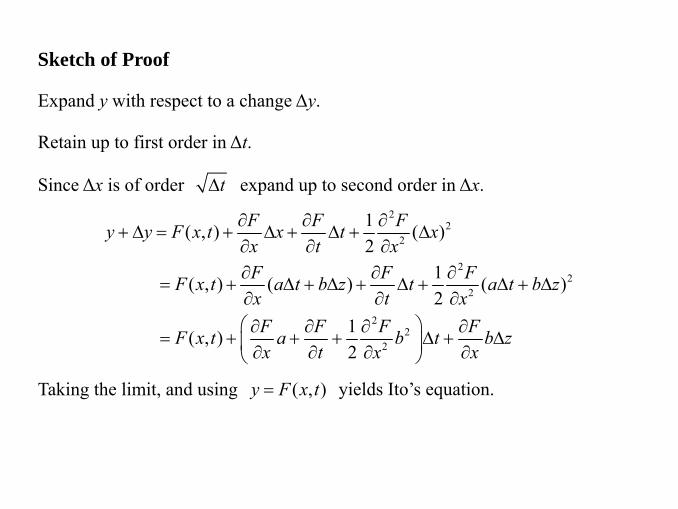
Sketch of Proof
Expand y with respect to a change Δy.
Retain up to first order in Δt.
Since Δx is of order tΔ expand up to second order in Δx. 2
22
22
2
22
2
1( , ) ( )2
1( , ) ( ) ( )2
1( , )2
F F Fy y F x t x t xx t xF F FF x t a t b z t a t b zx t xF F F FF x t a b t b zx t x x
∂ ∂ ∂+ Δ = + Δ + Δ + Δ
∂ ∂ ∂∂ ∂ ∂
= + Δ + Δ + Δ + Δ + Δ∂ ∂ ∂⎛ ⎞∂ ∂ ∂ ∂
= + + + Δ + Δ⎜ ⎟∂ ∂ ∂ ∂⎝ ⎠
Taking the limit, and using ( , )y F x t= yields Ito’s equation.
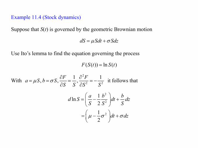
Example 11.4 (Stock dynamics)
Suppose that S(t) is governed by the geometric Brownian motion
dS Sdt Sdzμ σ= +
Use Ito’s lemma to find the equation governing the process
( ( )) ln ( )F S t S t=
With 2
2 2
1 1, , ,F Fa S b SS S S S
μ σ ∂ ∂= = = = −
∂ ∂ it follows that
2
2
2
1ln2
12
a b bd S dt dzS S S
dt dzμ σ σ
⎛ ⎞= − +⎜ ⎟
⎝ ⎠⎛ ⎞ = − +⎜ ⎟⎝ ⎠
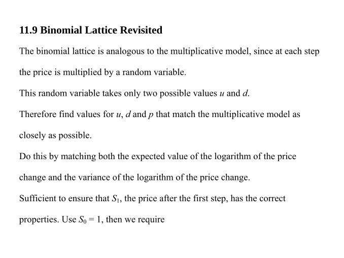
11.9 Binomial Lattice Revisited
The binomial lattice is analogous to the multiplicative model, since at each step
the price is multiplied by a random variable.
This random variable takes only two possible values u and d.
Therefore find values for u, d and p that match the multiplicative model as
closely as possible.
Do this by matching both the expected value of the logarithm of the price
change and the variance of the logarithm of the price change.
Sufficient to ensure that S1, the price after the first step, has the correct
properties. Use S0 = 1, then we require
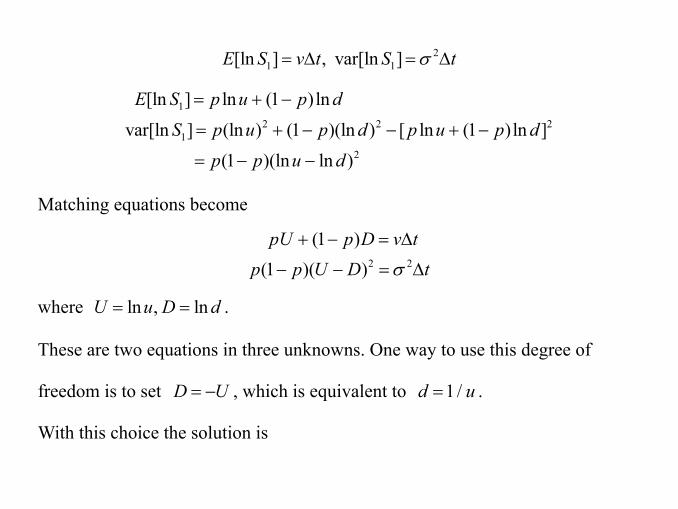
21 1[ln ] , var[ln ]E S v t S tσ= Δ = Δ
12 2 2
12
[ln ] ln (1 )ln
var[ln ] (ln ) (1 )(ln ) [ ln (1 )ln ]
(1 )(ln ln )
E S p u p d
S p u p d p u p d
p p u d
= + −
= + − − + −
= − −
Matching equations become
2 2
(1 )(1 )( )pU p D v t
p p U D tσ
+ − = Δ
− − = Δ
where ln , lnU u D d= = .
These are two equations in three unknowns. One way to use this degree of
freedom is to set D U= − , which is equivalent to 1 /d u= .
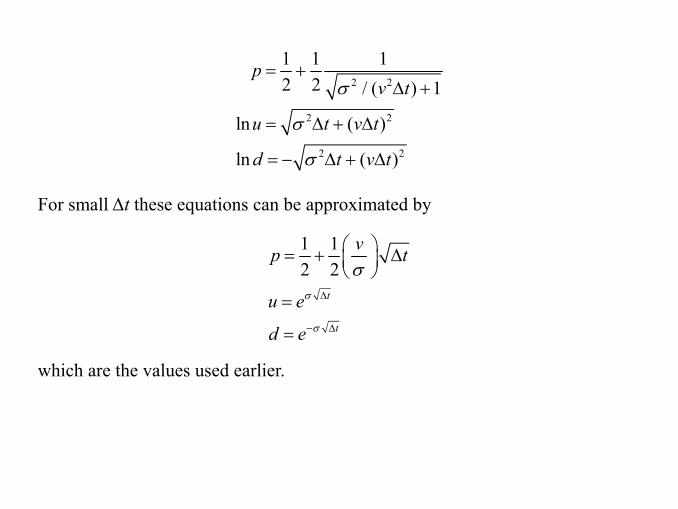
With this choice the solution is
2 2
2 2
2 2
1 1 12 2 / ( ) 1
ln ( )
ln ( )
pv t
u t v t
d t v t
σ
σ
σ
= +Δ +
= Δ + Δ
= − Δ + Δ
For small Δt these equations can be approximated by
1 12 2
t
t
vp t
u e
d e
σ
σ
σΔ
− Δ
⎛ ⎞= + Δ⎜ ⎟⎝ ⎠
=
=
which are the values used earlier.
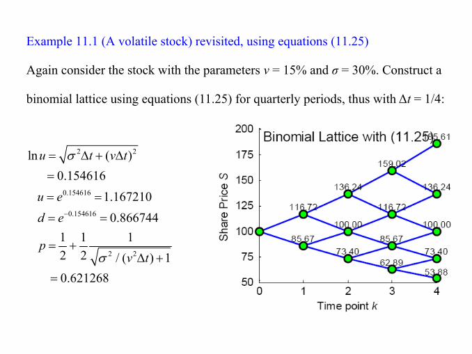
Example 11.1 (A volatile stock) revisited, using equations (11.25)
Again consider the stock with the parameters ν = 15% and σ = 30%. Construct a
binomial lattice using equations (11.25) for quarterly periods, thus with Δt = 1/4:
2 2
0.154616
0.154616
2 2
ln ( )0.154616
1.1672100.866744
1 1 12 2 / ( ) 10.621268
u t v t
u ed e
pv t
σ
σ
−
= Δ + Δ
=
= =
= =
= +Δ +
=

Critical assumptions
• Share price described by geometric Brownian motion.• Can constantly adjust hedging ratio with negligible dealing costs.• Share has infinite liquidity, ie we can buy or sell any amount we want instantly.• The interest rate is known for the duration of the option - reasonableif over a few months.• The volatility can be estimated accurately.
Come back to these later - meantime assume they are satisfied.
Note that we have not assumed any particular type of financial derivative, so the equation has very general applicability.

在模型推导中,假定市场处理想状态,且:
μ和扩散项 分别为常数的随机过程; 1.股票价格遵循漂移项 σ
r
2.允许使用全部所得卖空衍生证券;
3.所有证券都是高度可分的;
4.在衍生证券的有效期内没有红利支付;
5.不存在无风险套利机会;
6.证券交易是连续的,没有交易费用或税收;
7.无风险利率 为常数且对所有到期日都相同。
当然这些条件可以在以后的讨论中逐步放宽,但是并不会影响
Black-Scholes 模型的完美性。
ECG590I Asset Pricing. Lecture 12: Black-Scholes 1
12 Black-Scholes
12.1 The fundamental PDEs
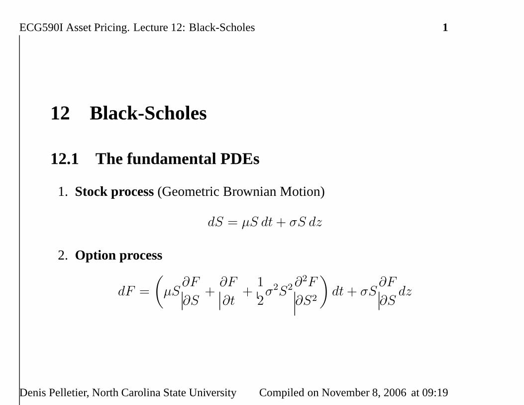
1. Stock process(Geometric Brownian Motion)
dS = µS dt + σS dz
2. Option process
dF =
(
µS∂F
∂S+
∂F
∂t+
1
2σ2S2∂2F
∂S2
)
dt + σS∂F
∂Sdz
Denis Pelletier, North Carolina State University Compiled on November 8, 2006 at 09:19
ECG590I Asset Pricing. Lecture 12: Black-Scholes 2
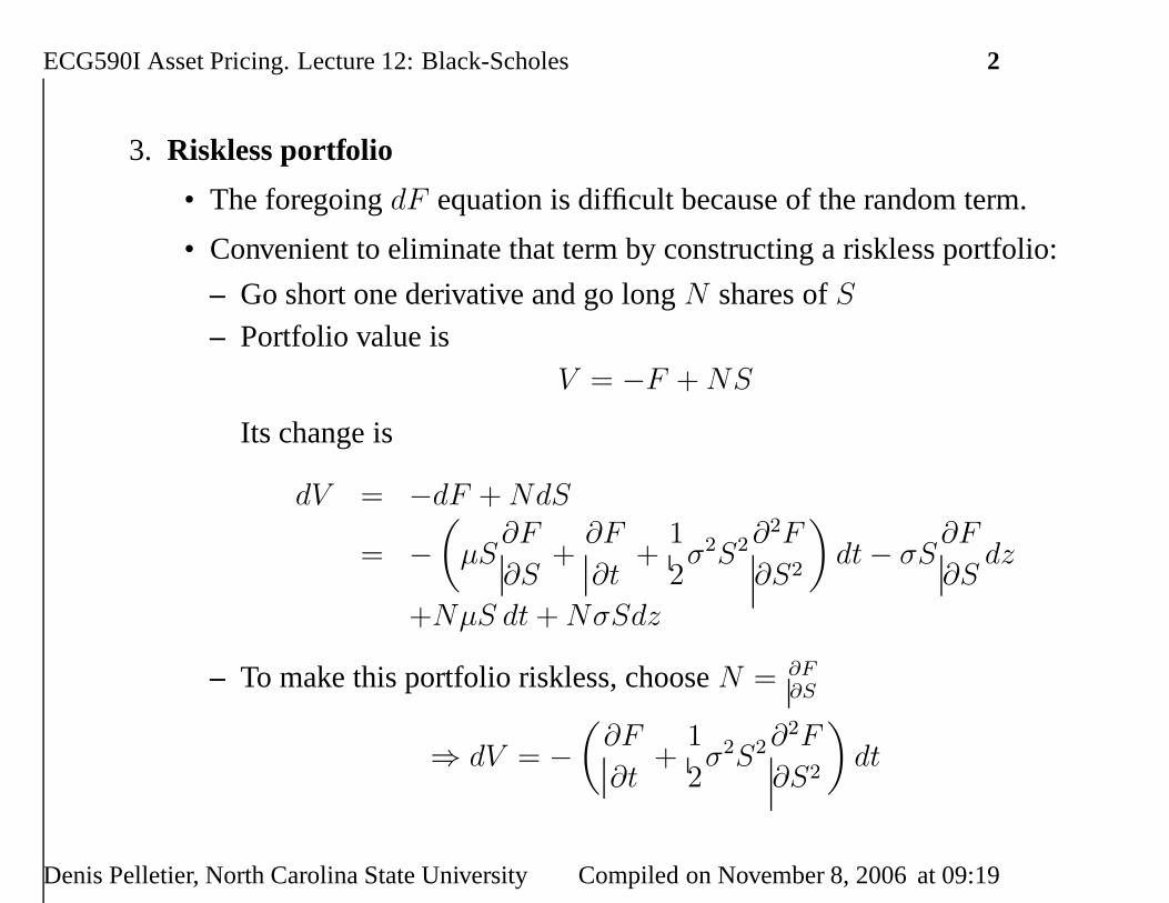
3. Riskless portfolio
• The foregoingdF equation is difficult because of the random term.
• Convenient to eliminate that term by constructing a riskless portfolio:
– Go short one derivative and go longN shares ofS– Portfolio value is
V = −F + NS
Its change is
dV = −dF + NdS
= −
(
µS∂F
∂S+
∂F
∂t+
1
2σ2S2∂2F
∂S2
)
dt − σS∂F
∂Sdz
+NµS dt + NσSdz
– To make this portfolio riskless, chooseN = ∂F∂S
⇒ dV = −
(
∂F
∂t+
1
2σ2S2∂2F
∂S2
)
dt
Denis Pelletier, North Carolina State University Compiled on November 8, 2006 at 09:19
ECG590I Asset Pricing. Lecture 12: Black-Scholes 3
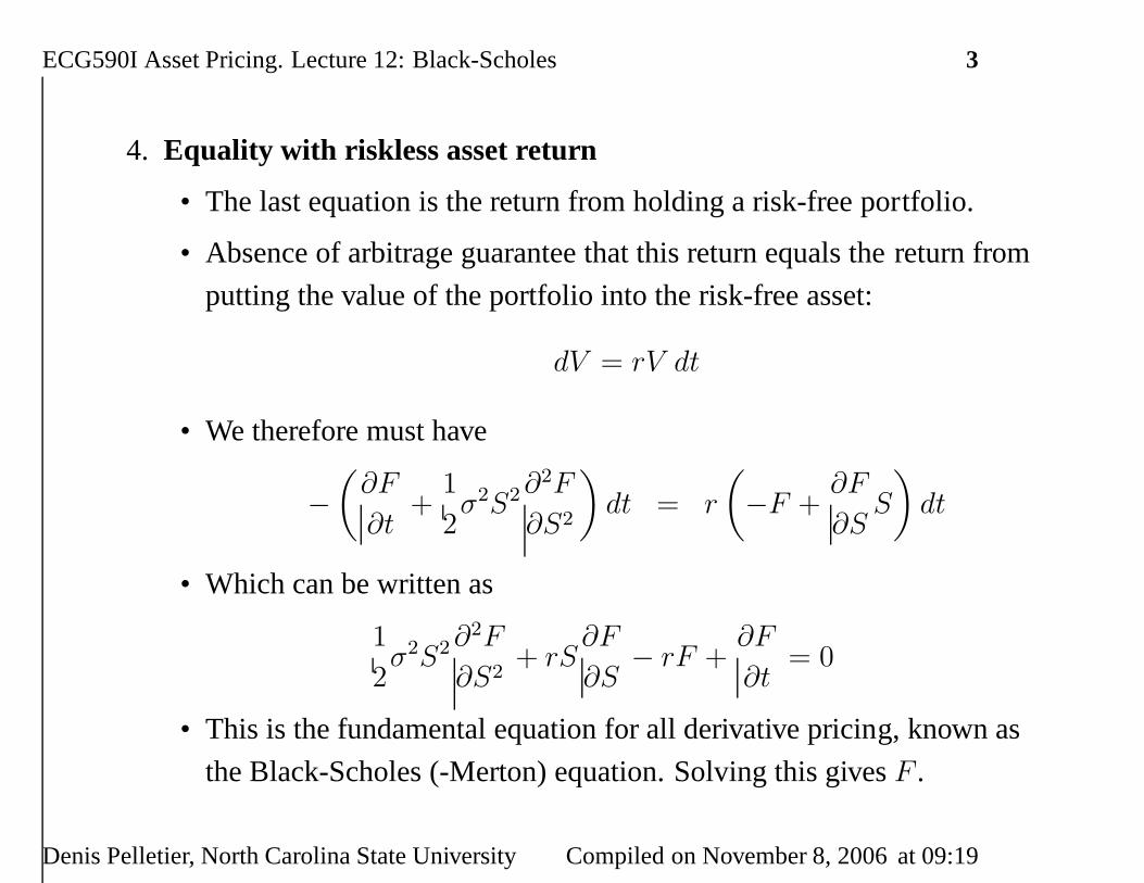
4. Equality with riskless asset return
• The last equation is the return from holding a risk-free portfolio.
• Absence of arbitrage guarantee that this return equals the return from
putting the value of the portfolio into the risk-free asset:
dV = rV dt
• We therefore must have
−
(
∂F
∂t+
1
2σ2S2∂2F
∂S2
)
dt = r
(
−F +∂F
∂SS
)
dt
• Which can be written as
1
2σ2S2∂2F
∂S2+ rS
∂F
∂S− rF +
∂F
∂t= 0
• This is the fundamental equation for all derivative pricing, known as
the Black-Scholes (-Merton) equation. Solving this givesF .
Denis Pelletier, North Carolina State University Compiled on November 8, 2006 at 09:19
ECG590I Asset Pricing. Lecture 12: Black-Scholes 4
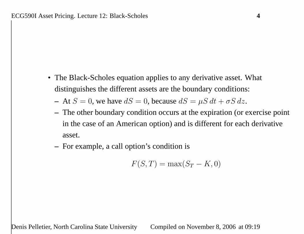
• The Black-Scholes equation applies to any derivative asset. What
distinguishes the different assets are the boundary conditions:
– At S = 0, we havedS = 0, becausedS = µS dt + σS dz.
– The other boundary condition occurs at the expiration (or exercise point
in the case of an American option) and is different for each derivative
asset.
– For example, a call option’s condition is
F (S, T ) = max(ST − K, 0)
Denis Pelletier, North Carolina State University Compiled on November 8, 2006 at 09:19

ECG590I Asset Pricing. Lecture 12: Black-Scholes 5
12.2 Solving the equation
1. Two approaches:
• PDE with boundary conditions
• Risk-neutral valuation (martingale theory). This approach is more
convenient for this problem.
2. Risk-neutral valuation
(a) Applies here because
• There is a finite stopping time (the expiration date)
• No element of investor risk preference enters the Black-Scholes
equation.
– Note in particular that the expected returnµ on the stock is
absent from the equation. The value ofµ does depend on
risk preferences.
Denis Pelletier, North Carolina State University Compiled on November 8, 2006 at 09:19
ECG590I Asset Pricing. Lecture 12: Black-Scholes 6
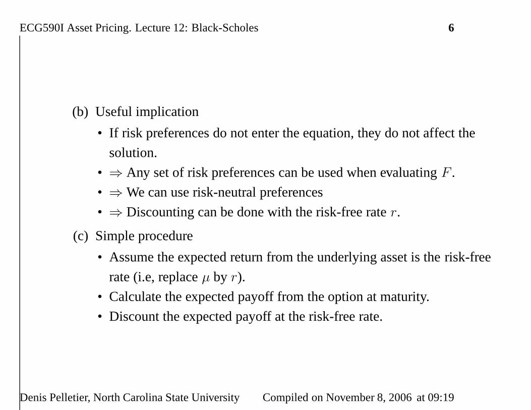
(b) Useful implication
• If risk preferences do not enter the equation, they do not affect the
solution.
• ⇒ Any set of risk preferences can be used when evaluatingF .
• ⇒ We can use risk-neutral preferences
• ⇒ Discounting can be done with the risk-free rater.
(c) Simple procedure
• Assume the expected return from the underlying asset is the risk-free
rate (i.e, replaceµ by r).
• Calculate the expected payoff from the option at maturity.
• Discount the expected payoff at the risk-free rate.
Denis Pelletier, North Carolina State University Compiled on November 8, 2006 at 09:19
ECG590I Asset Pricing. Lecture 12: Black-Scholes 7
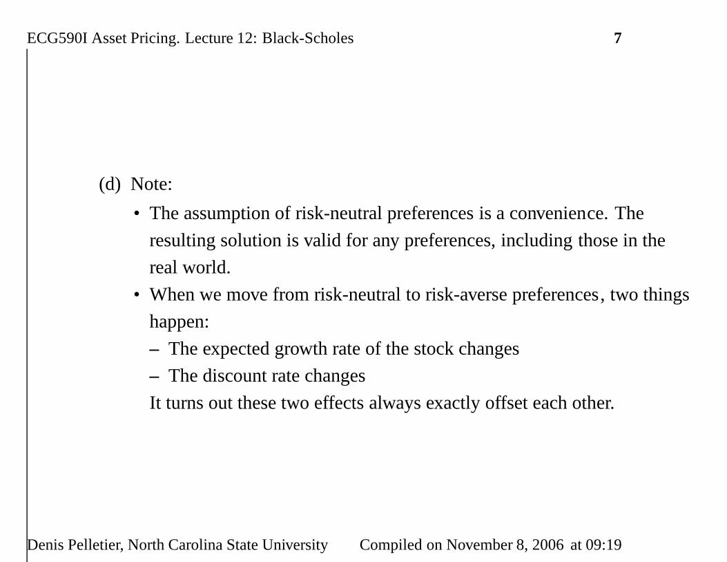
(d) Note:
• The assumption of risk-neutral preferences is a convenience. The
resulting solution is valid for any preferences, including those in the
real world.
• When we move from risk-neutral to risk-averse preferences, two things
happen:
– The expected growth rate of the stock changes
– The discount rate changes
It turns out these two effects always exactly offset each other.
Denis Pelletier, North Carolina State University Compiled on November 8, 2006 at 09:19
ECG590I Asset Pricing. Lecture 12: Black-Scholes 8
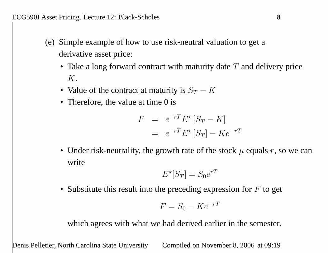
(e) Simple example of how to use risk-neutral valuation to get aderivative asset price:
• Take a long forward contract with maturity dateT and delivery priceK.
• Value of the contract at maturity isST − K
• Therefore, the value at time 0 is
F = e−rT E⋆ [ST − K]
= e−rT E⋆ [ST ] − Ke−rT
• Under risk-neutrality, the growth rate of the stockµ equalsr, so we canwrite
E⋆[ST ] = S0erT
• Substitute this result into the preceding expression forF to get
F = S0 − Ke−rT
which agrees with what we had derived earlier in the semester.
Denis Pelletier, North Carolina State University Compiled on November 8, 2006 at 09:19

Call option formula
The formula uses the function ( )N x , the standard cumulative normal
probability distribution. This is the cumulative distribution of a normal
random variable having mean 0 and variance 1. It can be expressed as 2
2
/ 2
' / 2
1( )21( )2
x y
x
N x e dy
N x e
π
π
−
−∞
−
=
=
∫
The function ( )N x is
illustrated in figure 11.1. The
value ( )N x is the area under
the familiar bell-shaped curve from −∞ to x. Particular values are
( ) 0, (0) 0.5, ( ) 1N N N−∞ = = ∞ = 。
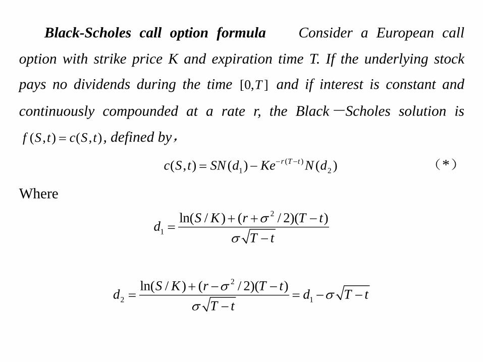
Black-Scholes call option formula Consider a European call
option with strike price K and expiration time T. If the underlying stock
pays no dividends during the time [0, ]T and if interest is constant and
continuously compounded at a rate r, the Black-Scholes solution is
( , ) ( , )f S t c S t= , defined by,
( )1 2( , ) ( ) ( )r T tc S t SN d Ke N d− −= − (*)
Where 2
1ln( / ) ( / 2)( )S K r T td
T tσ
σ+ + −
=−
2
2 1ln( / ) ( / 2)( )S K r T td d T t
T tσ σ
σ+ − −
= = − −−
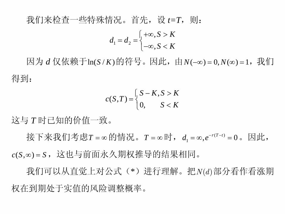
我们来检查一些特殊情况。首先,设 t=T,则:
1 2
,,S K
d dS K
+∞ >⎧= = ⎨−∞ <⎩
因为 d 仅依赖于ln( / )S K 的符号。因此,由 ( ) 0, ( ) 1N N−∞ = ∞ = ,我们
得到: ,
( , )0, S K S K
c S TS K
− >⎧= ⎨ <⎩
这与 T 时已知的价值一致。
接下来我们考虑T = ∞的情况。T = ∞时, ( )1 , 0r T td e− −= ∞ = 。因此,
( , )c S S∞ = ,这也与前面永久期权推导的结果相同。
我们可以从直觉上对公式(*)进行理解。把 ( )N d 部分看作看涨期
权在到期处于实值的风险调整概率。
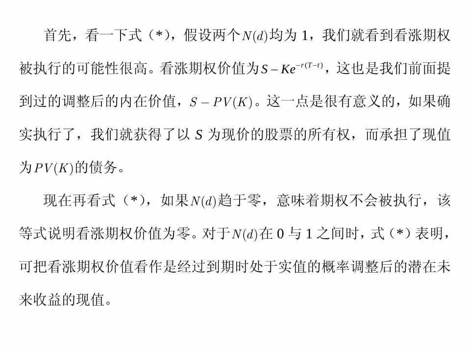
首先,看一下式(*),假设两个 ( )N d 均为 1,我们就看到看涨期权
被执行的可能性很高。看涨期权价值为 ( )r T tS Ke− −− ,这也是我们前面提
到过的调整后的内在价值, ( )S PV K− 。这一点是很有意义的,如果确
实执行了,我们就获得了以 S 为现价的股票的所有权,而承担了现值
为 ( )PV K 的债务。
现在再看式(*),如果 ( )N d 趋于零,意味着期权不会被执行,该
等式说明看涨期权价值为零。对于 ( )N d 在 0 与 1 之间时,式(*)表明,
可把看涨期权价值看作是经过到期时处于实值的概率调整后的潜在未
来收益的现值。

那么, ( )N d 又是如何表示风险调整概率的呢?这需要用到高级统
计学的知识。
注意ln( / )S K ,在 d1和 d2的分子中都出现了,它近似表示期权现在
实值与虚值的百分比。分母 T tσ − ,用股票价格在剩余期限中的标准
差对期权的实值与虚值的百分比进行调整。
如果股价变动很小,并且距到期的时间也所剩无几的时候,给定
比例的实值期权一般会保持原实值状态,因此, 1( )N d 与 2( )N d 代表期权
到期时处于实值的概率。
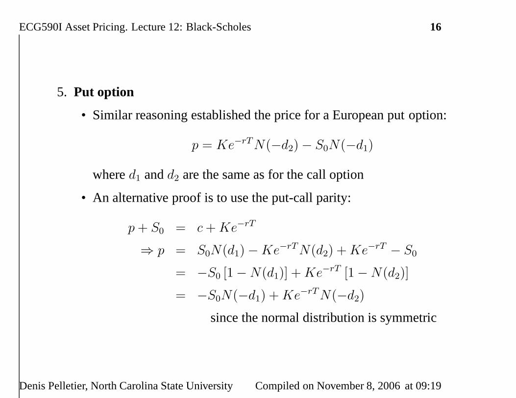
ECG590I Asset Pricing. Lecture 12: Black-Scholes 16
5. Put option
• Similar reasoning established the price for a European put option:
p = Ke−rT N(−d2) − S0N(−d1)
whered1 andd2 are the same as for the call option
• An alternative proof is to use the put-call parity:
p + S0 = c + Ke−rT
⇒ p = S0N(d1) − Ke−rT N(d2) + Ke−rT − S0
= −S0 [1 − N(d1)] + Ke−rT [1 − N(d2)]
= −S0N(−d1) + Ke−rT N(−d2)
since the normal distribution is symmetric
Denis Pelletier, North Carolina State University Compiled on November 8, 2006 at 09:19