models for a fair humanitarian relief distribution - … · models for a fair humanitarian relief...

Models for a Fair Humanitarian Relief Distribution Ana Maria Anaya-Arenas Angel Ruiz Jacques Renaud

March 2016

CIRRELT-2016-11 Document de travail également publié par la Faculté des sciences de l’administration de l’Université Laval, sous le numéro FSA-2016-003.

Models for a Fair Humanitarian Relief Distribution

Ana Maria Anaya-Arenas, Angel Ruiz*, Jacques Renaud

Interuniversity Research Centre on Enterprise Networks, Logistics and Transportation (CIRRELT) and Department of Operations and Decision Systems, 2325 de la Terrasse, Université Laval, Québec, Canada G1V 0A6

Abstract. Fairness has recently become a key concern for crisis managers. In the

aftermath of a disaster, when needs overcome response’s capacity, decision makers are

expected to distribute the available relief efficiently, but also in such a way that nobody

might perceive any injustice in the access to relief. This paper presents three multi-period

models to support relief distribution decisions. The models consider fairness but also

tackle the demand’s and offer’s changes over time. In addition, demand can be

backordered as it is the case in realistic situations. The paper discusses the notion of

fairness and proposes several proxies to measure it. Numerical tests are run on a set of

academic instances to analyze the behaviour of the considered models and assess their

performance.

Keywords: Emergency logistics, network design problem, relief distribution, fairness.

Acknowledgements. This research was partially supported by Grants OPG 0293307 and

OPG 0172633 from the Natural Sciences and Engineering Research Council of Canada

(NSERC) this support is gratefully acknowledged.

Results and views expressed in this publication are the sole responsibility of the authors and do not necessarily reflect those of CIRRELT.

Les résultats et opinions contenus dans cette publication ne reflètent pas nécessairement la position du CIRRELT et n'engagent pas sa responsabilité. _____________________________ * Corresponding author: [email protected]

Dépôt légal – Bibliothèque et Archives nationales du Québec Bibliothèque et Archives Canada, 2016

© Anaya-Arenas, Ruiz, Renaud and CIRRELT, 2016

1. Introduction

In the past decade, the number of scientific contributions on relief distribution has grown

significantly and nowadays humanitarian logistics has become an independent and important

body of research. In particular, relief distribution logistics, have many characteristics that

differentiates them from business logistics (Holguín-Veras et al. 2012; Kovács & Spens 2007).

Among them, three major features inspire and motivate this work. Firstly, demand is uncertain

and it may evolve very quickly as the population might tend to mobilize after a disaster. Thus

multi-period models are needed to tackle the demand’s dynamics. Secondly, relief distribution

logistics focuses on demand satisfaction rather than profit maximization or costs minimization,

because if the relief demand is not satisfied in terms of both quantities and time, the safety and

well-being of the affected people are jeopardized. Thirdly, relief must be distributed in a “fair”

manner among the people in need (Anaya-Arenas et al. 2014; Holguín-Veras et al. 2012;

Holguín-Veras et al. 2013). Our concern on justice in distribution was also promoted by Fujitsu

Consulting (Canada) Inc., one of our previous partners in emergency logistics developments. Past

results on design and planning of relief distribution (Rekik et al. 2013) showed that when the

response’s capacity is smaller than demand, and if fairness is not seek explicitly in the

optimization models, some PoDs can be completely neglected while others are fully covered.

This behavior was rejected by our partner, understanding then the importance of the principals of

justice and impartiality for humanitarian decision makers.

This paper proposes two main contributions. Firstly, we propose a multi-period formulation for

the design of a relief distribution network where the opening decisions of humanitarian aid

distribution centers (HADC), and the allocation of demand to the HACDs, are reconsidered at

every period. In addition, because of the limited amounts of relief available, we allow the demand


CIRRELT-2016-11 1

to be backordered, although only for a limited time or number of periods. A limited backorder of

demand allows us to provide a more flexible and realistic logistic plan. Secondly, since this

network must be planned in such a way that it maximizes fairness in the distribution, three

different objective functions will be proposed and their performance assessed using a set of

metrics.

The rest of this article is organized as follows. Section 2 reports the most relevant works in the

literature. Section 3 presents a discussion on the notion of fairness, and what we expect from a

fair relief distribution plan. Section 4 states the addressed problem. Section 5 presents three

different mathematical formulations for fair distribution network design and operations. Section 6

presents numerical experiments, while Section 7 concludes this work and suggests research

perspectives.

2. Fair relief distribution in humanitarian logistics

Relief distribution logistics (also called post disaster humanitarian logistics) have received

increasing attention in recent years. For instance, in their review, Anaya-Arenas et al. (2014)

reported 83 articles, from which 76 were published after 2004. However, the most recent works

claim that despite of the important contributions made up to date, additional efforts must be made

in order to truly understand the complexity of relief distribution and capturing the challenges of

disaster response in optimization models.

One of these challenges is to capture the variety of managers’ objectives. According to Anaya-

Arenas et al. (2014)’s review of the existing literature, 50% of the relief distribution literature

focuses on cost minimization. However, the acknowledgment of saving lives as the ultimate

purpose of relief distribution motivates the proposition of different objectives as satisfaction of


2 CIRRELT-2016-11

demand (20% of the literature) or rapidity of the response (20%). To the best of our knowledge,

only 10% of the literature on relief distribution networks has considered the fairness concept, and

it is almost exclusively done from a routing problems’ perspective. For instance, Tzeng et al.

(2007) proposed a multi-objective optimization problem for a transportation problem. Fairness of

distribution is the third objective, after cost and rapidity, and it is sought by maximizing the

minimum satisfaction level among clients. Suzuki (2012) used a similar approach. Lin et al.

(2011) also proposed a transportation problem for relief distribution with three different

objectives, and it is pursued by the minimization of the maximum gap of the unsatisfied demand.

Vitoriano et al. (2010; 2009) proposed a multi-criteria optimization model as well, where fairness

is sought by minimizing the deviation of normalized unsatisfied demands. The model considered

both costs and routes’ reliability. Finally, Huang et al. (2012) presented three different ways to

measure what they call equity. The first approach computed a deviation measure like the one

used in Lin et al. (2011) and Tzeng et al. (2007). The second one measured the standard deviation

of the demand satisfaction using a non-linear formulation. The third approach used a piecewise-

linear function to penalize inequity. They tested the three approaches on a set of routing instances

and compared their efficiency. Only two contributions on the relief distribution network design

literature included the fairness objective. Lin et al. (2012) included a penalty cost for unfairness

in service in its cost minimization objective function to design temporal depots in the affected-

area, and Yushimito et al. (2012) used an economic function including social cost. As we can see,

the use of fairness objectives is still spare, and the most common approach for it is a deviation

minimization. However, we will show how other cost functions can indeed be more efficient, as

it was presented by Huang et al. (2012) and Holguín-Veras et al. (2013).


CIRRELT-2016-11 3

Holguín-Veras et al. (2013) is one of the few works to underline the need for objective functions

to represent the real challenge of post-disaster humanitarian logistic models. They discussed how

social costs must be included in the objective function, in addition to the logistics cost. To do it, a

monotonic, non-linear and convex cost function, in respect to the deprivation time, is proposed to

estimate the human suffering caused by the supplies’ deficit of goods or services to a community

in the aftermath of a disaster. Their contribution was later extended in Pérez-Rodríguez and

Holguín-Veras (2015) were this proposition was applied for a routing and inventory allocation

problem. Through their analysis, they underlined the opportunity cost linked to the satisfaction of

clients’ demand and the need for multi-period models that account for the temporal effect of

demand’s dissatisfaction. These two aspects are highly important for the development of a fair

distribution chain and are therefore captured in our proposition.

Although several objectives are pursued when designing and operating a relief distribution

network, the fairness objective is the major focus of our work. This is due to its significance and

rareness, which also makes this principle the hardest one to define and measure. The next section

discusses fairness and how to apply and measure it in a relief distribution network design.

3. What should be expected and how to measure fairness in relief

distribution?

Relief distribution decisions need to be anchored in the principle of fairness and justice. The

principle of justice is based on how each person has an inviolability founded on justice that even

the welfare of society as a whole cannot override (Rawls 2009). In the context of goods or relief

distribution, several aspects need to be observed. First, in terms of demand satisfaction, equity

should be pursued. The term equity implies that everyone’s demand will be satisfied to the same


4 CIRRELT-2016-11

proportion, according to their needs. Since each point of demand (PoD) may require a different

amount of help, equity should be measured as a percentage of satisfied demand or, alternatively,

as a percentage of the demand’s shortage. Furthermore, this idea of equity in demand satisfaction

(or dissatisfaction) needs to be refined in a dynamic, multiperiod context. What we mean by this

is that, even if all the PoDs have the same percentage of demand satisfaction at the end of the

planning horizon, the way in which they receive relief during the planning horizon is of

paramount importance. Clearly, a fair relief distribution should ensure that every PoD maintains a

supply level as close as possible, not only to its total needs, but to its needs at each period. It

follows that eventual shortages should be “distributed” in a fair manner among the PoD and,

whenever there is a shortage at a given PoD, it should be “compensated” as soon as possible.

Finally, response time should be, in the best possible way, the same for every PoD, and this

interest is beyond a distance minimization objective. Of course, geography and population

distribution make this goal very difficult to attain, but a fairness’s perception can be reinforced by

ensuring that every PoD can be supplied in less than a given time by at least one open HADC.

The next subsection discusses how to assess the fairness of a given distribution plan.

Fairness metrics 3.1.

Beamon and Balcik (2008) developed a complete framework for performance measurement

inspired by commercial supply chains. They suggested that a good relief distribution network

needs to achieve a high performance in efficiency, effectiveness and flexibility. They recognised

the need of fairness, but they did not specify any indicator or proxy related to it.

We believe that in a multiperiod context, fairness needs to be achieved within the same period,

and across periods. With fairness within periods we aim at minimizing the differences on the


CIRRELT-2016-11 5

percentage of demand satisfaction between PoDs in a given period. Consequently, if there is a

shortness at a given period 𝑡, it is preferred to deliver to each customer an equal fraction of their

demand rather than fully satisfy some PoDs while leaving others suffering important shortages.

On the other hand, fairness across periods refers to how the distribution plan balances eventual

shortages by “rationing” the available supplies among the PoDs during the planning horizon. In

other words, it might be preferable to deliver PoDs with a portion of their demand, rather than to

fully satisfy demand in a period and fully unsatisfying it in another. In the following, we name

the fairness within periods as “equity” and fairness across periods as “stability”. Aiming at

quantifying the fairness of a given distribution plan, we define four measures on the differences

in shortage among the deserved PoDs. These measures are based on the range and the dispersion

and specifically concern equity and stability.

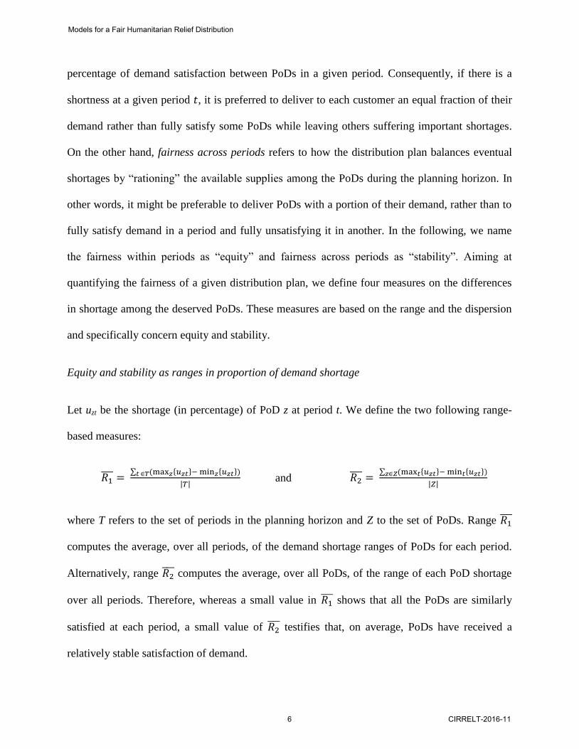
Equity and stability as ranges in proportion of demand shortage

Let uzt be the shortage (in percentage) of PoD z at period t. We define the two following range-

based measures:

𝑅1 =

∑ (max𝑧{𝑢𝑧𝑡}− min𝑧{𝑢𝑧𝑡})𝑡 ∈𝑇

|𝑇| and 𝑅2

= ∑ (max𝑡{𝑢𝑧𝑡}− min𝑡{𝑢𝑧𝑡})𝑧∈𝑍

|𝑍|

where T refers to the set of periods in the planning horizon and Z to the set of PoDs. Range 𝑅1

computes the average, over all periods, of the demand shortage ranges of PoDs for each period.

Alternatively, range 𝑅2 computes the average, over all PoDs, of the range of each PoD shortage

over all periods. Therefore, whereas a small value in 𝑅1 shows that all the PoDs are similarly

satisfied at each period, a small value of 𝑅2 testifies that, on average, PoDs have received a

relatively stable satisfaction of demand.


6 CIRRELT-2016-11

Equity and stability in terms of global dispersion

Variance and standard deviation are measures used to quantify the dispersion of a set of data

around its average value. Let us define 𝑢.. as the global average of the demand shortage over all

PoDs and all periods (in percentage), and 𝜎2𝑔𝑙𝑜𝑏𝑎𝑙 be the shortage’s global variance over all

PoDs and periods computed as:

𝜎2𝑔𝑙𝑜𝑏𝑎𝑙 =

∑ ∑ (𝑢𝑧𝑡 − 𝑢∙∙)2

𝑧 ∈𝑍𝑡 ∈𝑇

|𝑇| × |𝑍| − 1

The following paragraphs show how a classic analysis of variance allows us to identify the

components of equity (within a period) and stability (across periods) in the relief distribution

decisions. The numerator of 𝜎2𝑔𝑙𝑜𝑏𝑎𝑙 is a Total Sum of Squares (TSS) of the deviations of the

shortages’ values from their average value. Taking periods as a main factor, TSS can be

decomposed in two independent terms: Sum of Squares Within periods (𝑆𝑆𝑊𝑇) and Between

periods (𝑆𝑆𝐵𝑇). This decomposition let us quantify how much of the global dispersion is due to

the variability inside (within) the periods and how much is due to the variability of distribution

decisions between the periods. More precisely,

∑ ∑ (𝑢𝑧𝑡 − 𝑢∙∙)2

𝑧 ∈𝑍𝑡 ∈𝑇 = 𝑇𝑆𝑆 = 𝑆𝑆𝑊𝑇 + 𝑆𝑆𝐵𝑇

with:

𝑆𝑆𝑊𝑇 = ∑ ∑ (𝑢𝑧𝑡 − 𝑢∙𝑡)2𝑧 ∈𝑍𝑡 ∈𝑇 and 𝑆𝑆𝐵𝑇 = |𝑍| ∑ (𝑢∙𝑡 − 𝑢∙∙)

2𝑡 ∈𝑇 ,

where 𝑢∙𝑡 is the average over all PoD’s of the shortage percentage for period t (i.e. 𝑢∙𝑡 =

∑ 𝑢𝑧𝑡𝑧 ∈𝑍 |𝑍|⁄ ). 𝑆𝑆𝑊𝑇 measures in the planning horizon if, period by period, the PoDs are all


CIRRELT-2016-11 7

similarly satisfied; therefore, it is the basic component of equity among PoDs. On his side, 𝑆𝑆𝐵𝑇

shows the dispersion of the average demand shortage per period around the global mean value

(𝑢..). Therefore, 𝑆𝑆𝐵𝑇 is related to the stability of the distribution decisions in time (all PoDs

combined). We believe that 𝑆𝑆𝐵𝑇 is a good measurement of how the distribution decisions are

able to “smooth” the supply variations in the planning horizon.

Since global variance (𝜎2𝑔𝑙𝑜𝑏𝑎𝑙) is computed by dividing TSS by its degrees of freedom (|𝑇| ×

|𝑍| − 1), one can find the mean value of each component by dividing it by its respective degree

of freedom. Therefore, and based in the previous decomposition analysis, it is possible to define

two dispersion measures, named 𝑊𝑇 , 𝐵𝑇 , as follows:

𝑊𝑇 =𝑆𝑆𝑊𝑇

|𝑇| × (|𝑍| − 1) and 𝐵𝑇 =

𝑆𝑆𝐵𝑇

|𝑇| − 1

It is worth mentioning that, although the variance decomposition presented in the previous

paragraphs uses periods as main factor, a similar decomposition could have been done using the

PoDs as the main factor. Indeed, doing so, the decomposition exercise would have led to two

alternative dispersion measures on stability (𝑊𝑍 ) and equity (𝐵𝑍 ) :

𝑊𝑍 =∑ ∑ (𝑢𝑧𝑡 − 𝑢𝑧∙)

2𝑧 ∈𝑍𝑡 ∈𝑇

|𝑍| × (|𝑇| − 1) and 𝐵𝑍 =

|𝑇| ∑ (𝑢𝑧∙ − 𝑢∙∙)2

𝑡 ∈𝑇

|𝑍| − 1

4. Problem definition and formulations

This section defines the considered distribution context and proposes three different mathematical

formulations that aimed tackling explicitly the notion of fairness in the satisfaction of the PoDs’

demand. We consider a multi period planning horizon composed of 𝑡 ∈ 𝑇 periods. The network


8 CIRRELT-2016-11

includes three types of nodes: the outside suppliers 𝑠 ∈ 𝑆, the potential HADCs 𝑙 ∈ 𝐿, and the

PoDs 𝑧 ∈ 𝑍. The exact location of all the nodes is known, and the transportation time between

each two nodes 𝑖 and 𝑗 is denoted 𝑐𝑖𝑗. We consider a set of different products’ families or relief’s

kits, named in the following humanitarian functions 𝑓 ∈ 𝐹 such as survival (e.g., meals, water),

safety, medical, technical, etc. (Rekik et al, 2013). We assume that each PoD 𝑧 has a given

demand 𝑑𝑧𝑓𝑡 for each particular function 𝑓 and period 𝑡, expressed in number of pallets or any

other standard measure.

If a PoD does not receive its complete demand for a given period, we assume that it can be

backordered and fulfilled within the next period. If the backordered demand is not delivered

during the next period, this demand is considered lost. We have fixed the limit of backordered

demand to one period, considering that compensating demand after more than one period can be

too late and cause as much damage as if demand is never delivered. Evidently, this can be

adjusted accordingly to the time’s discretization used and the needs of the crisis managers. Please

notice that the formulation can be easily extended to consider two periods of backorder or more.

On the other side, allowing backorders gives flexibility to managers, but it must be avoided

whenever possible. To reflect this, we establish a penalty cost 𝛽1𝑓 if the demand for a function 𝑓

is delayed by one period, and 𝛽2𝑓 if demand is lost, with 𝛽2𝑓 ≫ 𝛽1𝑓.

Each HADC 𝑙 has a specific global capacity limit by period (𝐺𝑙𝑜𝑏𝑙𝑡) and a capacity limit by

function (𝐶𝑎𝑝𝐷𝑙𝑓𝑡), also by period. This capacity is expressed in number of pallets. On the other

hand, suppliers’ capacity is also limited to a number of pallets for each function at each period

(𝐶𝑎𝑝𝑆𝑠𝑓𝑡). Finally, each HADC needs a specific number of professionals (𝑛𝑙) to operate at its

full capacity. However, there is a restriction on the total number of personnel 𝑁𝑡 available at each


CIRRELT-2016-11 9

period 𝑡, which in fact limits the total number of HADC to open. Also, the opening of an HADC

requires some setting-up activities, decreasing in practice the center’s available operation time for

the period. We therefore assume that, during the period when a center is open, its capacity of

incoming and outgoing flow is reduced by a factor α < 1. Contrariwise, a center can be closed at

any period without any additional cost.

The transportation of relief (from suppliers to HADCs and finally from HADCs to PoDs) is

assumed to be done by truckloads of capacity 𝑃 (same vehicle type). A transportation capacity

limit is established for both the number of trips between a supplier 𝑠 and a center 𝑙 (𝑉𝑠𝑠𝑙), as well

as the number of trips between a pair of HADC 𝑙 and PoD 𝑧 (𝑉𝑑𝑙𝑧) at any period.

The proposed optimization models seek to define a relief distribution network focusing in three

primary aspects. First, we seek to minimize the demand shortage while maximizing fairness. The

secondary objective (efficiency) is achieved by minimizing the total travel time, affecting directly

the allocation decisions. Lastly, rapidity in distribution is not included in the objective function,

but assured using maximum access time constraints for the supply (τ1) and the distribution (τ2).

In the following, we introduce additional notation and then we present common constraints for

the three models. Finally, each of the alternative objective functions are proposed. Notice that all

the quantities as well as capacities are expressed in pallets, but they can be expressed using any

other standard measure.

Sets

𝑆𝑙 Set of suppliers within the maximum distance of HADC 𝑙 (𝑠 ∈ 𝑆𝑙 ∶ 𝑐𝑠𝑙 ≤ 𝜏1);

𝐿𝑠 Set of HADCs that are within the maximum distance of supplier 𝑠 (𝑙 ∈ 𝐿𝑠 ∶ 𝑐𝑠𝑙 ≤ 𝜏1);

𝐿𝑧 Set of HADCs that are within the maximum distance of PoD 𝑧 ( 𝑙 ∈ 𝐿𝑧 : 𝑐𝑙𝑧 ≤ 𝜏2);


10 CIRRELT-2016-11

𝑍𝑙 Set of PoDs that are within the maximum distance of HADC 𝑙 (𝑧 ∈ 𝑍𝑙 ∶ 𝑐𝑙𝑧 ≤ 𝜏2);

Decisions variables

𝑥𝑡𝑙 binary variable equal to 1 if the HADC 𝑙 is open at period 𝑡, zero otherwise;

𝑦𝑡𝑙 binary variable equal to 1 if the HADC 𝑙 is operating at period 𝑡, zero otherwise;

𝑄𝑠𝑠𝑙𝑓𝑡 quantity of function 𝑓 sent from supplier 𝑠 to HADC 𝑙 at the beginning of period 𝑡;

𝑄𝑑𝑙𝑧𝑓𝑡 quantity of function 𝑓 sent from HADC 𝑙 ∈ 𝐿𝑧 to PoD 𝑧 ∈ 𝑍 during period 𝑡;

𝑆𝑧𝑓𝑡,𝑡+1− quantity of function 𝑓 not delivered at PoD 𝑧 during period 𝑡, scheduled to be delivered

at period t + 1;

𝑆𝑧𝑓𝑡,𝑡+2− quantity of function 𝑓 not delivered at PoD 𝑧 during period 𝑡, and that will not be

delivered at the end of period 𝑡 + 1, so it is counted as lost demand;

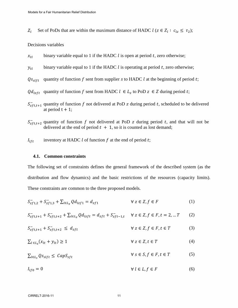
𝐼𝑙𝑓𝑡 inventory at HADC 𝑙 of function 𝑓 at the end of period 𝑡;

Common constraints 4.1.

The following set of constraints defines the general framework of the described system (as the

distribution and flow dynamics) and the basic restrictions of the resources (capacity limits).

These constraints are common to the three proposed models.

𝑆𝑧𝑓1,2− + 𝑆𝑧𝑓1,3

− + ∑ 𝑄𝑑𝑙𝑧𝑓1𝑙∈𝐿𝑧= 𝑑𝑧𝑓1 ∀ 𝑧 ∈ 𝑍, 𝑓 ∈ 𝐹 (1)

𝑆𝑧𝑓𝑡,𝑡+1− + 𝑆𝑧𝑓𝑡,𝑡+2

− + ∑ 𝑄𝑑𝑙𝑧𝑓𝑡𝑙∈𝐿𝑧= 𝑑𝑧𝑓𝑡 + 𝑆𝑧𝑓𝑡−1,𝑡

− ∀ 𝑧 ∈ 𝑍, 𝑓 ∈ 𝐹, 𝑡 = 2, … 𝑇 (2)

𝑆𝑧𝑓𝑡,𝑡+1− + 𝑆𝑧𝑓𝑡,𝑡+2

− ≤ 𝑑𝑧𝑓𝑡 ∀ 𝑧 ∈ 𝑍, 𝑓 ∈ 𝐹, 𝑡 ∈ 𝑇 (3)

∑ (𝑥𝑙𝑡 + 𝑦𝑙𝑡)𝑙 ∈𝐿𝑧≥ 1 ∀ 𝑧 ∈ 𝑍, 𝑡 ∈ 𝑇 (4)

∑ 𝑄𝑠𝑠𝑙𝑓𝑡𝑙∈𝐿𝑠≤ 𝐶𝑎𝑝𝑆𝑠𝑓𝑡 ∀ 𝑠 ∈ 𝑆, 𝑓 ∈ 𝐹, 𝑡 ∈ 𝑇 (5)

𝐼𝑙𝑓0 = 0 ∀ 𝑙 ∈ 𝐿, 𝑓 ∈ 𝐹 (6)


CIRRELT-2016-11 11

𝐼𝑙𝑓𝑡 = 𝐼𝑙𝑓𝑡−1 + ∑ 𝑄𝑠𝑠𝑙𝑓𝑡𝑠∈𝑆𝑙− ∑ 𝑄𝑑𝑙𝑧𝑓𝑡𝑧∈𝑍𝑙

∀ 𝑙 ∈ 𝐿, 𝑓 ∈ 𝐹, 𝑡 ∈ 𝑇 (7)

∑ 𝐼𝑙𝑓𝑡𝐹𝑓 ≤ 𝐺𝑙𝑜𝑏𝑙𝑡(𝑥𝑙𝑡 + 𝑦𝑙𝑡) ∀ 𝑙 ∈ 𝐿, 𝑡 ∈ 𝑇 (8)

𝐼𝑙𝑓𝑡 ≤ 𝐶𝑎𝑝𝐷𝑙𝑓𝑡 ∀ 𝑙 ∈ 𝐿, 𝑓 ∈ 𝐹, 𝑡 ∈ 𝑇 (9)

∑ 𝑄𝑠𝑠𝑙𝑓𝑡𝐹𝑓

𝑃≤ 𝑉𝑠𝑠𝑙𝑡(𝛼𝑥𝑙𝑡 + 𝑦𝑙𝑡) ∀ 𝑠 ∈ 𝑆𝑙, 𝑙 ∈ 𝐿, 𝑡 ∈ 𝑇 (10)

∑ 𝑄𝑑𝑙𝑧𝑓𝑡𝐹𝑓

𝑃 ≤ 𝑉𝑑𝑙𝑧𝑡(𝛼𝑥𝑙𝑡 + 𝑦𝑙𝑡) ∀ 𝑧 ∈ 𝑍𝑙 , 𝑙 ∈ 𝐿, 𝑡 ∈ 𝑇 (11)

∑ 𝑛𝑙(𝑥𝑙𝑡 + 𝑦𝑙𝑡)𝐿𝑙 ≤ 𝑁𝑡 ∀ 𝑡 ∈ 𝑇 (12)

𝑥𝑙𝑡 + 𝑦𝑙𝑡 ≤ 1 ∀ 𝑙 ∈ 𝐿, 𝑡 ∈ 𝑇 (13)

𝑦𝑙𝑡 ≤ 𝑥𝑙𝑡−1 + 𝑦𝑙𝑡−1 ∀ 𝑙 ∈ 𝐿, 𝑡 = 2 … 𝑇 (14)

𝑦𝑙𝑡−1 + 𝑥𝑙𝑡 ≤ 1 ∀ 𝑙 ∈ 𝐿, 𝑡 = 2 … 𝑇 (15)

𝑥𝑙𝑡−1 + 𝑥𝑙𝑡 ≤ 1 ∀ 𝑙 ∈ 𝐿, 𝑡 = 2 … 𝑇 (16)

𝑥𝑙𝑡, 𝑦𝑙𝑡 = {0,1} ∀ 𝑙 ∈ 𝐿, 𝑡 ∈ 𝑇 (17)

𝑆𝑧𝑓𝑡,𝑡+1− , 𝑆𝑧𝑓𝑡,𝑡+2

− , 𝑄𝑠𝑙𝑓𝑡, 𝑄𝑙𝑧𝑓𝑡, 𝐼𝑙𝑓𝑡, ≥ 0 ∀ 𝑠 ∈ 𝑆𝑙 𝑧 ∈ 𝑍𝑙 , 𝑙 ∈ 𝐿, 𝑓 ∈ 𝐹,

𝑡 ∈ 𝑇

(18)

Constraints set (1) defines the quantity of the humanitarian function 𝑓 not delivered to PoD 𝑧 at

period 1, which are scheduled to be delivered at period 2 or will be considered as lost. This

equation is generalized in constraints (2) for the other periods. Constraints (3) limit the quantity

that can be backordered (or lost) for a given period to the demand of the period. These constraints

also assure that backordered demand is delivered during the period where it is expected.

Constraints (4) require that an active HADC (opened or already in operation) within the covering

distance of each PoD must be open at every period. Constraints (5) state that the total flow of a

given function sent to the HADCs from a given supplier 𝑠 at period 𝑡 must respect the supplier’s


12 CIRRELT-2016-11

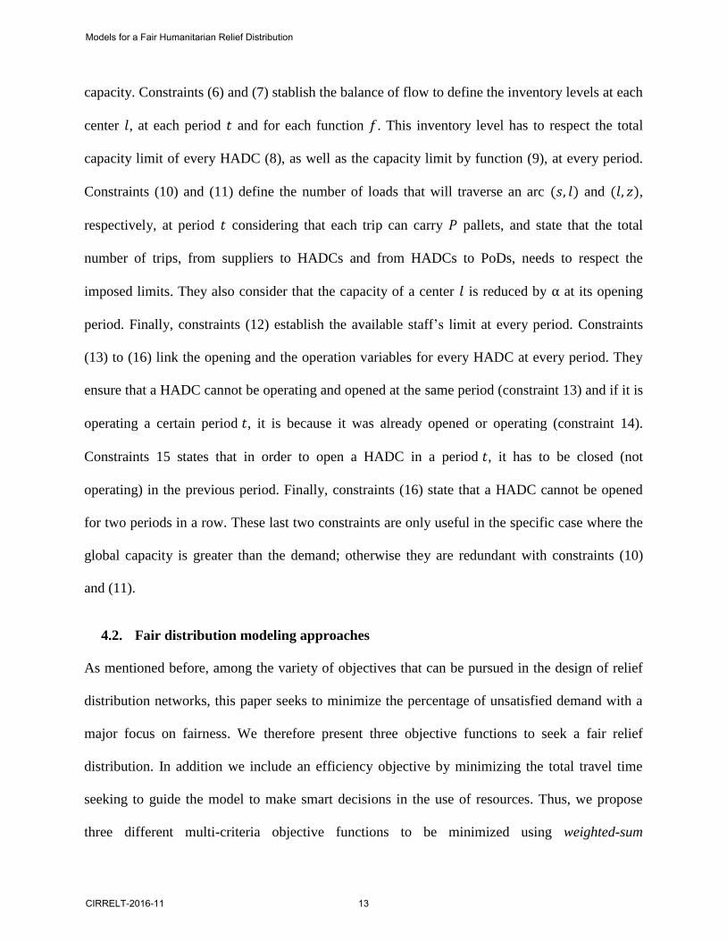
capacity. Constraints (6) and (7) stablish the balance of flow to define the inventory levels at each

center 𝑙, at each period 𝑡 and for each function 𝑓. This inventory level has to respect the total

capacity limit of every HADC (8), as well as the capacity limit by function (9), at every period.

Constraints (10) and (11) define the number of loads that will traverse an arc (𝑠, 𝑙) and (𝑙, 𝑧),

respectively, at period 𝑡 considering that each trip can carry 𝑃 pallets, and state that the total

number of trips, from suppliers to HADCs and from HADCs to PoDs, needs to respect the

imposed limits. They also consider that the capacity of a center 𝑙 is reduced by α at its opening

period. Finally, constraints (12) establish the available staff’s limit at every period. Constraints

(13) to (16) link the opening and the operation variables for every HADC at every period. They

ensure that a HADC cannot be operating and opened at the same period (constraint 13) and if it is

operating a certain period 𝑡, it is because it was already opened or operating (constraint 14).

Constraints 15 states that in order to open a HADC in a period 𝑡, it has to be closed (not

operating) in the previous period. Finally, constraints (16) state that a HADC cannot be opened

for two periods in a row. These last two constraints are only useful in the specific case where the

global capacity is greater than the demand; otherwise they are redundant with constraints (10)

and (11).

Fair distribution modeling approaches 4.2.

As mentioned before, among the variety of objectives that can be pursued in the design of relief

distribution networks, this paper seeks to minimize the percentage of unsatisfied demand with a

major focus on fairness. We therefore present three objective functions to seek a fair relief

distribution. In addition we include an efficiency objective by minimizing the total travel time

seeking to guide the model to make smart decisions in the use of resources. Thus, we propose

three different multi-criteria objective functions to be minimized using weighted-sum


CIRRELT-2016-11 13

optimization method. The details of each objective function and the additional constraints

required for each model are presented in the following.

4.2.1. M1: Minimization of the penalty associated to the total unsatisfied demand

The first model is one of the most popular in relief distribution. It concentrates in minimizing the

penalty due to the unsatisfied demand. However, this approach has been adapted to account for

backordered and lost demand. Finally, it includes the efficiency objective of minimizing total

travel time. To present this three objectives in a single objective function, each term 𝑖 is affected

by a penalty factor δ𝑖. Let 𝑢𝑧𝑓𝑡 be the percentage of unsatisfied demand of humanitarian function

𝑓 at PoD 𝑧 in period 𝑡, if any. We define Obj1 (19) as the penalty cost for the percentage of

unsatisfied demand penalized by factor δ1; Obj2 (20) is the penalty cost of backordered and lost

demand penalized by factor δ2; and Obj3 (21) is the cost associated with the number of trips

multiplied by their distance and penalized by factor δ3. Each objective is formulated as follows:

𝑂𝑏𝑗1 = 𝛿1(∑ ∑ ∑ 𝑢𝑧𝑓𝑡𝑓 ∈𝐹𝑧∈𝑍 𝑡 ∈ 𝑇 ) (19)

𝑂𝑏𝑗2 = 𝛿2 (∑ ∑ ∑ 𝛽1𝑓

𝑆𝑧𝑓𝑡,𝑡+1−

𝑑𝑧𝑓𝑡𝑓 ∈𝐹𝑧∈𝑍 𝑡 ∈ 𝑇 + ∑ ∑ ∑ 𝛽2𝑓


𝑑𝑧𝑓𝑡𝑓 ∈𝐹𝑧∈𝑍 𝑡 ∈ 𝑇 )

(20)

𝑂𝑏𝑗3 = 𝛿3 (∑ ∑ ∑ 𝑐𝑠𝑙

∑ 𝑄𝑠𝑠𝑙𝑓𝑡𝐹𝑓

𝑃𝑙 ∈𝐿𝑠 ∈ 𝑆 𝑡 ∈ 𝑇 + ∑ ∑ ∑ 𝑐𝑙𝑧

∑ 𝑄𝑑𝑙𝑧𝑓𝑡𝐹𝑓

𝑃𝑧 ∈ 𝑍𝑙 ∈ 𝐿 𝑡 ∈ 𝑇 ) (21)

Model 1 (M1) is then formulated as:

Min 𝑂𝑏𝑗1 + 𝑂𝑏𝑗2 + 𝑂𝑏𝑗3 (22)

subject to:

𝑢𝑧𝑓𝑡 ≥ 1 −∑ 𝑄𝑑𝑙𝑧𝑓𝑡𝑙∈𝐿𝑧

𝑑𝑧𝑓𝑡 ∀ 𝑧 ∈ 𝑍, 𝑓 ∈ 𝐹, 𝑡 = 1, … 𝑇 (23)

𝑢𝑧𝑓𝑡 ∈ [0,1] ∀ 𝑧 ∈ 𝑍, 𝑓 ∈ 𝐹, 𝑡 ∈ 𝑇 (24)

in addition to constraints (1) to (18) .


14 CIRRELT-2016-11

4.2.2. M2: Minimization of the maximum gap

The second approach to maximize distribution fairness is similar to the one in Tzeng (2007) and

Lin et al. (2011). It consists in minimizing the largest gap among the unsatisfied demand (in

percentage) for all pairs of zones. We have adapted and extended this approach to take

backorders into account. Let 𝛾𝑓𝑡,𝑡+1 be the maximum gap between PoDs of the percentage of

demand of humanitarian function 𝑓 that is backordered at period 𝑡 to be payed at period 𝑡 + 1.

Likewise, we define 𝛾𝑓𝑡,𝑡+2 as the maximum gap among the PoDs of the percentage of demand of

humanitarian function 𝑓 that is lost at period 𝑡. We thus define Obj4 (25) as the penalty cost for

unsatisfied demand’s range, penalized by factor 𝛿4 and we add constraints (27) and (28) to the

model.

𝑂𝑏𝑗4 = 𝛿4(∑ ∑ 𝛽1𝑓𝛾𝑓𝑡,𝑡+1 + 𝛽2𝑓𝛾𝑓𝑡,𝑡+2𝑓 ∈𝐹𝑡 ∈ 𝑇 ) (25)

In this model we include also the minimization of backorders and lost demands and total travel

time as presented in M1 (𝑂𝑏𝑗2 and 𝑂𝑏𝑗3)

The second model (M2) can be stated as follows:

Min 𝑂𝑏𝑗4 + 𝑂𝑏𝑗2 + 𝑂𝑏𝑗3 (26)

Subject to:

𝑆𝑖𝑓𝑡,𝑡+1−

𝑑𝑖𝑓𝑡−

𝑆𝑗𝑓𝑡,𝑡+1−

𝑑𝑗𝑓𝑡≤ 𝛾𝑓𝑡,𝑡+1 ∀ 𝑖, 𝑗 ∈ 𝑍 (𝑖 ≠ 𝑗 ), 𝑓 ∈ 𝐹, 𝑡 ∈ 𝑇 (27)

𝑆𝑖𝑓𝑡,𝑡+2−

𝑑𝑖𝑓𝑡−

𝑆𝑗𝑓𝑡,𝑡+2−

𝑑𝑗𝑓𝑡 ≤ 𝛾𝑓𝑡,𝑡+2 ∀ 𝑖, 𝑗 ∈ 𝑍 (𝑖 ≠ 𝑗 ), 𝑓 ∈ 𝐹, 𝑡 ∈ 𝑇 (28)

in addition to constraints (1) to (18).


CIRRELT-2016-11 15

M3: Minimum dissatisfaction cost with a piecewise penalty function

We were inspired by Holguín-Veras et al. (2013) and Huang et al. (2012), which suggested the

use of a monotonic, non-linear and convex function to express the cost associated to human

suffering caused by the deficit of supplies or services in the aftermath of a disaster. Indeed, the

perception of the people in need is clearly not linear, and higher values of dissatisfaction of

demand must be penalized more strongly than lower values. In a similar manner, delays of two

periods in demand’s satisfaction has a larger cost (penalty) than twice the penalty for one period

delay. We propose to model penalties related to the percentage of unsatisfied demand as an

exponential function. Using non-linear penalties in the objective function is a way to seek

fairness. In order to introduce such effect in our model while keeping its linearity, we

approximated the penalty curve for a given unsatisfied demand percentage of PoD 𝑧,

humanitarian function 𝑓 at period 𝑡 (i.e. 𝑢𝑧𝑓𝑡) by a piecewise linear function as depicted in Figure

1, where it can be observed that the penalty increases significantly from one piece 𝑘 to the next

one. We refer the reader interested in the mathematical aspects of this linearization to Padberg

(2000).

Figure 1 – Example of a piecewise cost function for 𝒖𝒛𝒇𝒕.


16 CIRRELT-2016-11

In addition, we need to adapt this approach to take backorders and lost demands into account. We

thus define Obj5 (29) as the piecewise penalty cost for the percentage of total dissatisfaction

percentage with a penalty weight of 𝛿5 and Obj6 (30) as the piecewise penalty cost for

backordered and lost demand percentage with a penalty weight of 𝛿6:

𝑂𝑏𝑗5 = 𝛿5 ∑ ∑ ∑ 𝑓 ∈ 𝐹𝑧 ∈ 𝑍 𝑡 ∈ 𝑇 [𝑓(𝑢𝑧𝑓𝑡𝑘)] (29)

𝑂𝑏𝑗6 = 𝛿6[𝛽1𝑓𝑓(𝑢𝑧𝑓𝑡,𝑡+1,𝑘) + 𝛽2𝑓𝑓(𝑢𝑧𝑓𝑡,𝑡+2,𝑘)] (30)

Then, we include the efficiency objective (𝑂𝑏𝑗3) as is done in M1 and M2. M3 can be stated as

follows:

𝑀𝑖𝑛 𝑂𝑏𝑗5 + 𝑂𝑏𝑗6 + 𝑂𝑏𝑗3 (31)

The first two terms of (31) accounts for the penalty associated to unsatisfied demand (as well as

the backorder and lost demand) for each product, each PoD and each period. This is given by the

piecewise linear function defined by the following functions:

𝑓(𝑢𝑧𝑓𝑡𝑘) = ∑ 𝑐𝑘 𝐾𝑘=1 𝑢𝑧𝑓𝑡𝑘 (32)

𝑓(𝑢𝑧𝑓𝑡,𝑡+1,𝑘) = ∑ 𝑐𝑘 𝐾𝑘=1 𝑢𝑧,𝑓,𝑡,𝑡+1,𝑘 (33)

𝑓(𝑢𝑧𝑓𝑡,𝑡+2,𝑘) = ∑ 𝑐𝑘 𝐾𝑘=1 𝑢𝑧,𝑓,𝑡,𝑡+2,𝑘 (34)

where 𝑢𝑧𝑓𝑡𝑘 ∈ [0, 𝑎𝑘 − 𝑎𝑘−1] is the percentage, of the demand of function 𝑓 not delivered to

PoD 𝑧 at period 𝑡, that is inside the piece 𝑘, 𝑐𝑘 is the slope of piece 𝑘 (𝑐𝑘 =𝑏𝑘−𝑏𝑘−1

𝑎𝑘−𝑎𝑘−1) and (𝑎𝑘, 𝑏𝑘)

is the breaking point of the piecewise function related to piece 𝑘 (same for backorder and lost

demand). The last term computes the penalty associated to distribution time as in the previous

models. Model M3 requires the following constraints (in addition to constraints (1) to (18)):


CIRRELT-2016-11 17

∑ 𝑢𝑧𝑓𝑡𝑘𝐾𝑘=1 ≥ 1 −

∑ 𝑄𝑑𝑙𝑧𝑓𝑡𝑙∈𝐿𝑧

𝑑𝑧𝑓𝑡 ∀ 𝑧 ∈ 𝑍, 𝑓 ∈ 𝐹, 𝑡 = 1, … 𝑇 (35)

∑ 𝑢𝑧,𝑓,𝑡,𝑡+1,𝑘𝐾𝑘=1 =


𝑑𝑧𝑓𝑡 ∀ 𝑧 ∈ 𝑍, 𝑓 ∈ 𝐹, 𝑡 = 1, … 𝑇 (36)

∑ 𝑢𝑧,𝑓,𝑡,𝑡+2,𝑘𝐾𝑘=1 =


𝑑𝑧𝑓𝑡 ∀ 𝑧 ∈ 𝑍, 𝑓 ∈ 𝐹, 𝑡 = 1, … 𝑇 (37)

𝑢𝑧𝑓𝑡𝑘 ≤ (𝑎𝑘 − 𝑎𝑘−1) ∀ 𝑧 ∈ 𝑍, 𝑓 ∈ 𝐹, 𝑡 = 1, … 𝑇, 𝑘 ∈ 𝐾 (38)

𝑢𝑧𝑓𝑡,𝑡+1,𝑘 ≤ (𝑎𝑘 − 𝑎𝑘−1) ∀ 𝑧 ∈ 𝑍, 𝑓 ∈ 𝐹, 𝑡 = 1, … 𝑇, 𝑘 ∈ 𝐾 (39)

𝑢𝑧𝑓𝑡,𝑡+2,𝑘 ≤ (𝑎𝑘 − 𝑎𝑘−1) ∀ 𝑧 ∈ 𝑍, 𝑓 ∈ 𝐹, 𝑡 = 1, … 𝑇, 𝑘 ∈ 𝐾 (40)

𝑢𝑧𝑓𝑡𝑘, 𝑢𝑧𝑓𝑡,𝑡+1,𝑘, 𝑢𝑧𝑓𝑡,𝑡+2,𝑘 ∈ [0,1] ∀ 𝑧 ∈ 𝑍, 𝑓 ∈ 𝐹, 𝑡 ∈ 𝑇 (41)

Constraints (35) to (37) link the piecewise variables and the demand shortage quantities,

computing the total percentage of unsatisfied demand, the demand backorder at periods t + 1 and

t + 2 (lost demand) respectively, divided by demand of period 𝑡. Notice that in the case of a

compensation (i.e. if backordered demand is paid in a given period 𝑡), the total delivery might be

higher than the demand of 𝑡. In this case, the dissatisfaction percentage is computed as null.

Constraints (38) to (40) ensure that variables 𝑢𝑧𝑡𝑓,𝑡+1,𝑘 and 𝑢𝑧𝑡𝑓,𝑡+2,𝑘 cannot be greater that the

length of interval 𝑘. These constraints, together with the objective function, force the sequential

use of each piece of the piecewise function for variables 𝑢𝑧𝑓𝑡𝑘, 𝑢𝑧𝑓𝑡,𝑡+1,𝑘, 𝑢𝑧𝑓𝑡,𝑡+2,𝑘 respectively.

Constraint set (41) define the domain for the piecewise variables. Needless to say, the quality of

the solutions produced by model M3 depends on the number and the bounds of the pieces used in

the piecewise function. Therefore, a heuristic procedure is proposed to find a good compromise

in this matter. This method is presented in the next paragraphs.


18 CIRRELT-2016-11

Iterative approach to construct the piecewise linear function 4.3.

The number of pieces in the piecewise linear function and their breakpoints have a strong

influence on the quality of the solution as well as on its solvability. Three considerations must be

kept in mind when designing the piecewise function. First, a better approximation of the

exponential function may be obtained by using more pieces, but by doing so the model becomes

more difficult to solve. Second, since the piecewise cost function is intended to enforce equity by

trying to group all PoDs in the same dissatisfaction level (the same piece) pieces should be small

enough. Third, the fairest value of unsatisfied demand depends on the offer/demand ratio of a

period and its evolution in time. In other words, the proper number and value of each piece can

differ according to the specific instance. We therefore propose a heuristic procedure to fix the

number of pieces, the bounds of each one as well as the slope of each piece by an iterative

approach.

In the following, we illustrate the algorithm used to set the piecewise function of a particular

humanitarian function 𝑓 (i.e. considering 𝑢𝑧𝑓𝑡 as 𝑢𝑧𝑡). The heuristic is initialized with only two

pieces per variable (|𝐾| = 2). We define 𝐴 as the set of breakpoints 𝑎𝑘. 𝐴 is initialized with the

minimum value of the ratio offer/demand in the horizon (named 𝑚𝑖𝑛𝑡 𝜌𝑡), seeking to fix an upper

bound of dissatisfaction i.e. 𝐴 = {0; min𝑡 𝜌𝑡 ; 1}. Then, M3 is solved to optimality and the

solution produced is analyzed in order to decide if new pieces should be added to the piecewise

function and the model solved again (next iteration).

At a given iteration 𝑖, the average unsatisfied demand’s percentage (𝑢..𝑖) and the global standard

deviation (𝜎𝑔𝑙𝑜𝑏𝑎𝑙𝑖 as defined in Section 3.1) of the present solution are computed. If 𝜎𝑔𝑙𝑜𝑏𝑎𝑙

𝑖 is

greater than the standard deviation goal (𝜎𝑤𝑎𝑛𝑡𝑒𝑑 set arbitrary to zero), three new pieces are


CIRRELT-2016-11 19

added around 𝑢..𝑖, with three new breakpoints added to set 𝐴 as {𝑢..

𝑖 −𝜎𝑔𝑙𝑜𝑏𝑎𝑙

𝑖

2; 𝑢..

𝑖 ; 𝑢..𝑖 +

𝜎𝑔𝑙𝑜𝑏𝑎𝑙𝑖

2}.

Slopes for all the pieces are recalculated. To this end, we set a base penalty value for the first

piece in the function, and then the slope for each piece is increased by 1.1 times the rate between

the highest and the lowest demand (i.e. 𝑐𝑘 = 𝑐𝑘−1 × 1.1 𝐷𝑚𝑎𝑥

𝐷𝑚𝑖𝑛 ). After the recalculating the cost

piecewise function, the model is redefined and solved again. If the new solution results in a

reduction in 𝜎𝑔𝑙𝑜𝑏𝑎𝑙𝑖 a new iteration 𝑖 + 1 begins. If no improvement is achieved, the same

procedure is applied over the backorder and lost demand variables. The procedure is repeated

until a given stop criterion is met (e.g. maximal number of iterations, or until the improvement

obtained with current iteration is not significant or null). At the end, the last solution is retained

and reported as the solution of M3. The Algorithm 1 allows us to adapt the shape of the piecewise

function dynamically.

Algorithm 1 – Procedure to construct our piecewise function.

1. Initialize: Set |K| = 2 with 𝐴 = {0; min𝑡 𝜌𝑡 ; 1}, 𝜎𝑔𝑙𝑜𝑏𝑎𝑙0 = ∞; 𝑖 = 0 and maxIter = 5.

2. Set 𝑖 = 𝑖 + 1, 𝑠 ← MIP Solution to optimality using 𝐴 as bounds, estimate 𝜎𝑔𝑙𝑜𝑏𝑎𝑙𝑖 and 𝑢..𝑖

3. If 𝜎𝑔𝑙𝑜𝑏𝑎𝑙𝑖 > 𝜎𝑤𝑎𝑛𝑡𝑒𝑑 and 𝜎𝑔𝑙𝑜𝑏𝑎𝑙

𝑖 < 𝜎𝑔𝑙𝑜𝑏𝑎𝑙𝑖−1 then

Go to step 4

else

Go to step 6.

4. Estimate breakpoints of three new pieces:

4.1. Fix breakpoint = 𝑢..𝑖− 𝜎𝑔𝑙𝑜𝑏𝑎𝑙

𝑖 2⁄

4.2. Fix breakpoint = 𝑢..𝑖

4.3. Fix breakpoint = 𝑢..𝑖+ 𝜎𝑔𝑙𝑜𝑏𝑎𝑙

𝑖 2⁄

5. If the new bounds defined do not exist in 𝐴 and 𝑖 ≤ 𝑚𝑎𝑥𝐼𝑡𝑒𝑟 , then

5.1 add the bounds to 𝐴

5.2 go to step 2;


20 CIRRELT-2016-11

else

Go to step 6.

6. Return 𝑠

5. Numerical experiments

This section seeks to examine and to analyse, through numerical experiments, the behaviour of

the three different modeling approaches for a fair relief distribution over different scenarios.

Problem generation and demand scenarios 5.1.

In order to test the models, a flexible instance generator was designed to define and create a large

variety of test scenarios. All the parameters specified in the following paragraphs can be adapted

to the needs of a particular problem. The size of an instance is defined by the cardinality of the

following sets: PoDs (|Z|), HADCs (|L|), suppliers (|S|), humanitarian functions (|F|), and the

number of periods in the planning horizon (|T|). A problem is defined over a total area (TA) of

[1000 × 900], inside of which we define an affected area (AA) of [600 × 500]. The PoDs’ and

HADCs’ location is randomly generated inside the AA, and the set of suppliers inside the TA, but

outside the AA. The demand for each PoD at the first period is randomly generated in the range

of [20;70] for every humanitarian function. The capacity of any HADC 𝑙 is set at 60% of the total

demand (𝐶𝑎𝑝𝐷𝑙𝑓𝑡 = 0.6 ∑ 𝑑𝑧𝑓𝑡𝑧∈𝑍 ). In all our numerical experiments we seek to represent our

main interest in minimizing the unsatisfied demand percentage and the fairness objective, which

has been overlooked in the past. Therefore, in M1 we applied δ1 ≫ δ2 ≫ δ3, with δ1 ≅ 100δ2 ≅

1000δ3; for M2 we applied δ4 ≫ δ2 ≫ δ3, with δ4 ≅ 100δ2 ≅ 1000δ3 and for M3 we applied

δ5 ≫ δ6 ≫ δ3, with δ5 ≅ 100δ6 ≅ 1000δ3.

Depending on the nature and the gravity of the event (demand) and the availability of resources

(number and capacity of responders), different supply scenarios can be considered. Following

that, we defined two basic theoretical scenarios.


CIRRELT-2016-11 21

Scenario 1 - Temporary shortness of resources

In the first periods in the aftermath of a disaster, the available resources are limited and vary from

one period to another on the planning horizon. In other words, periods of shortness alternate with

others showing reasonable offer levels corresponding to the arrival of help from national and

international organizations. In this case, the backordering of the unsatisfied demand becomes an

interesting solution available to crisis managers.

Scenario 2: Extreme shortness of resources

In this scenario, the available supplies, in addition to the foreseen arrivals of relief, will be

systematically under the requirements. Crisis managers cannot make a commitment towards

future deliveries to compensate for the shortness. In this case, crisis managers would try to

distribute the available relief in the most fair manner.

We model both of our instances’ scenarios for a particular humanitarian function on an

offer/demand ratio 𝜌𝑡 for each time periods. In temporary shortness, suppliers have the capacity

to respond to the demand during the first periods. Then, 𝜌𝑡 drops under one when local supplies

are finished, and finally external supplies start to arrive (𝜌𝑡 > 1). In extreme shortness, we

consider that, during the first periods, local capacity is limited (𝜌𝑡 ≈ 0.8), and then it decreases

until a deep strong (𝜌𝑡 ≈ 0.2). In the following, numerical results produced for temporary

shortness are presented, followed by those produced for extreme shortness.

Models’ performance in a temporary shortness scenario 5.2.

In order to characterize the behavior of the solutions produced by the three models with respect to

fairness, we will use in this section a set of 10 small instances (two suppliers, three HADCs, six


22 CIRRELT-2016-11

PoDs, one humanitarian function, and eight periods). Instances were solved to optimality with

Gurobi v.6.0 for M1, M2, and M3. This later is solved several times according to the iterative

heuristic described in section 4.3.

We have thoroughly analyzed the solutions produced to the first instance I1 where 𝜌𝑡, the

offer/demand ratio at each period, is set to {1.0; 1.0; 0.7; 0.5; 0.9; 1.2; 1.2;1.2}. In other words,

after two periods in which the demand can be satisfied, there is a three periods shortness where

the offer falls to only 70% and then to 50% of the demand. From period five, offer rises to 90%

of the demand and, during the last three periods, it exceeds the requirements. Figure 2 shows the

dissatisfaction percentage at each PoD and period in the solutions produced by M1 (leftmost

chart), M2 (central chart) and M3 (rightmost chart) and how they behave in very different

manners.

Figure 2 – Dissatisfaction percentage for instance I1

If we look at how shortage is shared between the PoDs for a given period, M2 and M3 split the

shortness in a rather homogeneous manner: all the PoDs suffer similar shortages. However, M1

concentrates shortages only on a few PoDs, and those will experience very high values of

dissatisfaction. For instance, PoD four’s demand is 100%, 50% and 50% unsatisfied in periods

two to four. If we now look at how the global shortage is handled in time, we observe that M1

and M2 simply distribute the available quantities at each period. However, M3 shows a more


CIRRELT-2016-11 23

elaborated behavior, which translates in a smoother distribution. In fact, M3 reserves some

quantities during periods one and two in order to minimize the impact of the shortage in periods

three to five. Doing so, the maximum dissatisfaction percentage suffered by any PoD and at any

period is under 20%, while in M1’s solution some PoDs experience up to 100% of unsatisfied

demand and in M2’s solution PoDs suffer up to 60%. The piecewise approximation achieves a

rationalization of resources, resulting in an equitable distribution among PoDs (the same or

almost the same dissatisfaction level) in a period, and this in a stable matter across time in the

shortness periods. To sum up, both M2 and M3’s solutions achieve a good “equity” between the

PoDs, but M3 is also able to achieve an excellent “stability”.

Let us now see how these behaviors are captured by the proposed numerical indicators. Table 1

reports the numerical results produced by models M1, M2 and M3. To measure the quality of the

distribution plan obtained by each model, we report two global measures: the global average

dissatisfaction percentage (𝑢..), and the global standard deviation (𝜎𝑔𝑙𝑜𝑏𝑎𝑙), which concerns to the

dispersion in distribution. Then, we also compute mean sum of squares within time (𝑊𝑇 ) and

between time (𝐵𝑇 ) and the two range indicators (𝑅1 and 𝑅2

). Finally, we calculate the total

traveled distance (𝐷) and record the total computation time to solve each model in seconds.

Let us consider first the results produced for I1. We observe that M1 achieves a lower value for

𝑢.. (i.e. a better global satisfaction). The reason is that, although all the three models distribute the

same quantity of help, M1 prefers to give slightly higher quantities to PoDs 5 and 6 because the

marginal impact of a single additional help unit is higher for PoDs with small demand. On the

other hand, doing so deteriorates the equity and stability objectives. In fact, M1 is clearly

outperformed by both M2 and M3 for almost all the others indicators (excluding 𝐵𝑇 in which M2


24 CIRRELT-2016-11

shows the poorest performance). As expected, concerning 𝜎𝑔𝑙𝑜𝑏𝑎𝑙 (global dispersion over all PoDs

and periods), M2 achieves 18% and is clearly dominated by M3, which produces only 9%. As per

range indicators, 𝑅1 and 𝑅2

show the poor performance of M1. M2 has a perfect score in terms of

equity (𝑅1 ) and M3 shows an almost equal performance, but M3 offers a better performance with

respect to stability (𝑅2 ). This particular behaviour is confirmed by the dispersion indicators.

Indeed, M2 and M3 achieve equal “perfect” scores for equity (𝑊𝑇 ), but M3 offers better results

for stability (𝐵𝑇 ). This result is easily explained by the cost function structure of M3. The fact

that the domain of 𝑢𝑧𝑓𝑡 is discretized in different pieces, with a higher cost function (slope) for

each successive piece, makes it possible to seek the same (or almost the same) dissatisfaction

percentage for each period, PoD and humanitarian function.

We now analyze the rest of the results in Table 1. Lines Avg. show the average values for each

column over the 10 instances and lines # best counts the number of instances in which the model

achieved the best value of the indicator.

Table 1 – Results produced for 10 small instances (temporary shortness).

𝒖.. 𝝈𝒈𝒍𝒐𝒃𝒂𝒍 𝑾𝑻 𝑩𝑻 𝑹𝟏 𝑹𝟐

D Sec.

I1

M1 9% 26% 6% 12% 37% 50% 364 0.2

M2 11% 18% 0% 21% 0% 50% 367 0.2

M3 11% 9% 0% 6% 1% 21% 371 0.6

Avg.

M1 9% 24% 5% 11% 35% 45% 1338 0.2

M2 11% 17% 0% 19% 0% 50% 1329 0.1

M3 11% 9% 0% 6% 3% 20% 1380 0.6

# best

M1 10 0 0 0 0 0 3 4

M2 0 0 10 0 10 0 7 7

M3 0 10 10 10 0 10 0 0

Globally speaking, results are quite similar to the ones produced for instance I1. M1

systematically achieves the best average percentage of unsatisfied demand but at the cost of a


CIRRELT-2016-11 25

very poor equity and stability performances. M2 offers the best performance with regards to 𝑅1 ,

but M3’s performance is always very close to M2’s. As expected, M3’s stability performance is

the best over the three models. To sum up, M2 and M3 achieve equal (perfect) scores for 𝑊𝑇

(equity indicator), but M3 offers better results when measuring stability (𝐵𝑇 ).

Before moving on to the experiments on extreme shortness scenario, let us say few words about

the efficiency of the produced solutions. Both M1 and M2 produce the shortest total distance for

three and seven instances. However, M3’s average total distance is only 3.9% higher than M2.

We can therefore conclude that an equitable and smooth distribution does not cost much in terms

of transportation efficiency.

Models’ performance in an extreme shortness scenario 5.3.

In an extreme shortness scenario, when resources are really scarce, assuring equity in a period

and across the horizon is of the highest importance, because rationalization is the only way to

minimize suffering and reduce disparity in the relief given to affected people.

To validate the behavior of the solutions produced by the three proposed models, we use the same

set of instances of section 5.2., but this time the offer/demand ratio 𝜌𝑡 per period was set to

{0.8, 0.8, 0.8, 0.6, 0.6, 0.2, 0.2, 0.6}. In the same way as it was done in previous section, we’ll use

a single instance (I11) as an illustrative example to carefully explain each model’s behavior.

Figure 3 shows the dissatisfaction percentage at each PoD and period for this instance.

Figure 3 – Dissatisfaction percentage for instance I11.


26 CIRRELT-2016-11

First, it can be observed that M1 never visits PoD4, which is the POD with the highest demand.

On the other hand, PoDs 5 and 6, the ones having the lowest demand, are always visited. PoD1 is

also strongly penalized and is not visited in six out of eight periods. We believe that this

behaviour should not be tolerated in practice. On its side, M2 shares the amount of relief

available, assuring equity at every period, but again, it is not able to balance deliveries between

periods. Hence, all PoDs suffer equivalent penuries, but theirs demand is fully met in some

periods and totally unsatisfied in others (periods 4 and 7). We consider this as a questionable

decision because the lowest offer/demand ratio on the horizon is 20%. Indeed, M3 is the only

formulation that allows for equity among PoDs and stability throughout time, thus reducing the

maximum non-satisfaction level from 80% to 54% (in period seven) and 42% in the other

periods. Table 2 reports the performance values achieved by the solutions produced by models

M1 to M3.

Table 2 – Results produced for 10 small instances (extreme shortness).


D Sec.

I11

M1 35% 46% 24% 8% 100% 33% 204 0.1

M2 42% 35% 0% 86% 0% 97% 219 0.0

M3 42% 5% 0% 2% 4% 16% 219 0.4

Avg.

M1 33% 46% 24% 4% 100% 22% 824 0.1

M2 42% 31% 0% 68% 0% 89% 813 0.1

M3 42% 5% 0% 2% 4% 14% 819 0.6

# best

M1 10 0 0 7 0 2 3 4

M2 0 0 10 0 10 0 6 6

M3 0 10 10 8 0 8 1 0

As expected, M1 achieves again the lowest total dissatisfaction value. M3 shows a total deviation

of only 5% while M1 and M2 produce values of up to 46% and 35%, respectively. Again, M2

shows a perfect balance for all the PoDs within the same period, and M3’s results are not far.

Indeed, M3 also achieves a perfect score of 0% for 𝑊𝑇 and only 4% for 𝑅1 . On the other hand,


CIRRELT-2016-11 27

M3 clearly outperforms both M1 and M2 in terms of distribution stability. We extend our

analysis to nine more random generated instances. The numerical results are reported in Table 2.

As in the temporary shortness case, M3 minimizes global deviation and offers the best possible

equity and stability performances at a negligible increase in the distribution distance.

Models’ performance in larger-sized instances 5.4.

We will dedicate the last part of this section to show the models’ performance over a set of 20

instances with a more realistic size. The objective is to test the models’ capacity to ensure a fair

distribution over a much larger set of PoDs, and to test, at the same time, the computational effort

of each model. Following the pattern described in section 5.2 and 5.3, we solve 10 instances for

temporary shortness and 10 instances for extreme shortness cases. For each scenario we test five

medium-size instances and five large-size instances. We define as “medium-size” instances with

a total of 20 PoDs, 10 potential HADCs, six suppliers, one humanitarian function and eight

periods. Large-size instances have 50 PoDs, 20 HADCs, six suppliers, one function and eight

periods. Table 3 and Table 4 summarize the results for the temporary and extreme shortness

scenarios respectively. In the following, we will concentrate our analysis to models M2 and M3,

because M1 shows still the poorest performance in most of the indicators. Table 3 and Table 4

confirm that the models’ behaviors follow the same line observed in the smaller instances. M2

and M3 achieved almost the same dissatisfaction percentage, but distributed the limited resources

in a very different way. M3 achieves the best score in average global dispersion of only 9% and

around 3% for the temporary and extreme shortness cases respectively. Therefore, we can

observe that increasing the number of PoDs did not have an impact in the quality of the solution.

M3 can still ensure an equitable distribution among PoDs as M2 does and a much stronger


28 CIRRELT-2016-11

stability in time. For the temporary shortness case, M3 has an 𝑅2 of only 19% vs. 49% for M2,

while for the extreme shortness case M3 has an 𝑅2 of only 4% vs. 93% and 76% for M2.

Table 3 – Results produced for larger-sized instances in temporary shortness.


D Sec.

Avg. over 5

medium instances

M1 9% 26% 6% 35% 62% 45% 3590 0.1

M2 11% 17% 0% 63% 0% 49% 3475 2.3

M3 11% 9% 0% 18% 3% 19% 4005 1.6

Avg. over 5

large instances

M1 9% 27% 6% 89% 62% 49% 8003 0.3

M2 11% 16% 0% 143% 0% 49% 7782 35.3

M3 10% 9% 0% 45% 4% 19% 8840 3.4

Table 4 – Results produced for larger-sized instances in extreme shortness.


D Sec.

Avg. over 5

medium instances

M1 33% 47% 23% 6% 100% 12% 2110 0.1

M2 43% 30% 0% 205% 0% 93% 2062 2.9

M3 42% 2% 0% 0% 4% 4% 2069 1.4

Avg. over 5

large instances

M1 33% 47% 22% 1% 100% 4% 4751 0.2

M2 42% 26% 0% 413% 0% 76% 4657 10.2

M3 42% 3% 0% 1% 5% 4% 4723 0.9

The numerical values previously reported show their sensibility with respect to the specific type

of the scenario considered. In the extreme shortness scenario the obtained values tend to be

higher than in the temporary shortness one. This is related to the variability of the offer/demand

ratio defining each type of scenario. Finally, let us take a second to analyze the computational

effort needed to solve larger instances. All the models can be solved to optimality in short time

(less than a minute in average), even for large instances. However, M2 shows a high variability in

CPU time, having a lot of trouble to close the optimality gap. For instance, in the temporary

shortness case (for large instances) M2 takes 35 seconds on average with a standard deviation of

27 seconds due to extremes values in three out of five instances, while M3 takes 3,4 seconds on


CIRRELT-2016-11 29

average with a standard deviation of only 0,4 seconds. We can conclude that M3 is the modeling

approach that best suits the different objectives set for the complex problem of relief distribution.

6. Conclusions and future research

In this paper we proposed and discussed three different approaches for the design and the

operation of a relief distribution network. This work is mainly centered in two important

components that had been overlooked in the past: the fairness principle and the multi-period

nature of relief distribution. We strongly believe that these major aspects need to be covered in

response logistics, and they need to be addressed from the beginning of the response plan (the

network design phase) in order to improve the other logistic tasks (procurement, delivery plans

and transportation problems). Three important contributions were made in the fair relief

distribution problem. First of all, a discussion on what can be defined as a fair distribution was

presented, concluding that in order to obtain fairness, crisis managers should warrant equity in

distribution within periods, but also, stability in delivery in the best possible way. In addition, we

considered and modeled shortness by including the possibility of backordered demand. This

allows crisis managers to gain flexibility in the distribution and seek compensation of unsatisfied

PoDs on the planning horizon. Secondly, we proposed and adapted five performance indicators to

measure the two components of fairness. Finally, we proposed and tested three different

formulations to handle the complex context of relief distribution. These formulations seek mainly

minimization of unsatisfied demand and effectiveness in distribution, but also two of them

explicitly include the fairness objective. We compared them in some numerical examples and

concluded that, M2 achieves a perfect score in equity in distribution in a single period, but is

unable to maintain a stable distribution on the planning horizon. We proved, on its side, that M3

accounts for both equity and stability.


30 CIRRELT-2016-11

Several promising research paths are currently being considered. For instance, the extension of

our proposition to include routing planning, supplying an integral planning tool to CMs in

response and preparedness of relief distribution.

Acknowledgements

This research was partially supported by Grants OPG 0293307 and OPG 0172633 from the

Canadian Natural Sciences and Engineering Research Council (NSERC). This support is

gratefully acknowledged.

References

Anaya-Arenas, A.M., Renaud, J. & Ruiz, A., 2014. Relief distribution networks: a systematic

review. Annals of Operations Research, 223(1), pp.53–79.

Beamon, B.M. & Balcik, B., 2008. Performance measurement in humanitarian relief chains.

International Journal of Public Sector Management, 21(1), pp.4–25.

Holguín-Veras, J., Hart, W.H., Jaller, M., Van Wassenhove, L.N., Pérez, N. & Wachtendorf, T.,

2012. On the unique features of post-disaster humanitarian logistics. Journal of Operations

Management, 30, pp.494–506.

Holguín-Veras, J., Pérez, N., Jaller, M., Van Wassenhove, L.N. & Aros-Vera, F., 2013. On the

appropriate objective function for post-disaster humanitarian logistics models. Journal of

Operations Management, 31(5), pp.262–280.

Huang, M., Smilowitz, K. & Balcik, B., 2012. Models for relief routing: Equity, efficiency and

efficacy. Transportation research part E: logistics and transportation review, 48(1), pp.2–18.

Kovács, G. & Spens, K., 2007. Humanitarian logistics in disaster relief operations. International

Journal of Physical Distribution & Logistics Management, 37(2), pp.99–114.

Lin, Y., Batta, R., Rogerson, P., Blatt, A. & Flanigan, M., 2011. A logistics model for emergency

supply of critical items in the aftermath of a disaster. Socio-Economic Planning Sciences,

45(4), pp.132 – 145.

Lin, Y., Batta, R., Rogerson, P.A., Blatt, A. & Flanigan, M., 2012. Location of temporary depots

to facilitate relief operations after an earthquake. Socio-Economic Planning Sciences. 46(2),

pp.112–123.


CIRRELT-2016-11 31

Padberg, M., 2000. Approximating separable nonlinear functions via mixed zero-one programs.

Operations Research Letters, 27(1), pp.1–5.

Rekik, M., Ruiz, A., Renaud, J., Berkoune, D. & Paquet, S., 2013. A decision support system for

humanitarian network design and distribution operations. In Humanitarian and Relief

Logistics: research issues, case studies and future trends. edited by Zeimpekis, V., and Ichoua,

S., and Minis, I., pp. 1–20. New York: Springer.

Suzuki, Y., 2012. Disaster-Relief Logistics With Limited Fuel Supply. Journal of Business

Logistics, 33(2), pp.145–157.

Tzeng, G.H., Cheng, H.J. & Huang, T.D., 2007. Multi-objective optimal planning for designing

relief delivery systems. Transportation Research Part E: Logistics and Transportation

Review, 43(6), pp.673–686.

Vitoriano, B., Ortuño, T., Tirado, G. & Montero, J., 2010. A multi-criteria optimization model for

humanitarian aid distribution. Journal of Global Optimization, pp.1–20.

Vitoriano, B., Ortuño, T. & Tirado, G., 2009. HADS, a goal programming-based humanitarian

aid distribution system. Journal of Multi-Criteria Decision Analysis, 16 (1-2), pp.55–64.

Yushimito, W.F., Jaller, M. & Ukkusuri, S., 2012. A Voronoi-based heuristic algorithm for

locating distribution centers in disasters. Networks and Spatial Economics, 12(1), pp.21–39.


32 CIRRELT-2016-11

models for a fair humanitarian relief distribution - … · models for a fair humanitarian relief...

Documents