modelling water and carbon canopy fluxes - opus at uts: home · modelling water and carbon canopy...
TRANSCRIPT

Modelling Water and Carbon Canopy
Fluxes
by
Rhys James Whitley
B.Sc in Applied Physics (Hons)
in the
Faculty of Science
Department of Environmental Sciences
A thesis submitted in fulfillment for the degree of Doctor of Philosophy
February 2011

Declaration of Authorship
I, RHYS JAMES WHITLEY, declare that this thesis titled, ‘MODELLING WATER AND
CARBON CANOPY FLUXES’ and the work presented in it are my own. I confirm that:
� This work was done wholly or mainly while in candidature for a research degree at
this University.
� Where any part of this thesis has previously been submitted for a degree or any
other qualification at this University or any other institution, this has been clearly
stated.
� Where I have consulted the published work of others, this is always clearly attributed.
� Where I have quoted from the work of others, the source is always given. With the
exception of such quotations, this thesis is entirely my own work.
� I have acknowledged all main sources of help.
� Where the thesis is based on work done by myself jointly with others, I have made
clear exactly what was done by others and what I have contributed myself.
Signed:
Date:
i

The thing the ecologically illiterate don’t realize about an ecosystem is that it’s a system.
A system! A system maintains a certain fluid stability that can be destroyed by a misstep
in just one niche. A system has order, a flowing from point to point. If something dams
the flow, order collapses. The untrained miss the collapse until too late. That’s why the
highest function of ecology is the understanding of consequences.
Kynes in ”Appendix I: The Ecology of Dune”
Excerpt from Dune by Frank Herbet

Acknowledgements
I must first express my gratitude and thanks to my supervisors, Prof Derek Eamus, Dr
Belinda Medlyn, Dr Melanie Zeppel and Dr Cate Macinnis-Ng, who have provided me
with the utmost support, encouragement, criticisms and friendship in undertaking this
cyclopean project. I am also deeply grateful to my previous supervisor Dr Nicholas Arm-
strong, who helped to start me on the road of mathematical modelling and has provided
support in his own time. I also express my thanks to my friends and fellow colleagues Dr
Daniel Taylor, Dr Isa Yunusa and Dr Remko Duursma (University of Western Sydney)
who have also provided invaluable support and advice in completing this work.
I would like to thank Dr Jason Berringer (Monash University), Dr Lindsay Hutley (Charles
Darwin University), Dr Anthony O’Grady (University of Tasmania) and Dr Oula Ghan-
noum (University of Western Sydney) for supplying the data that has made this work
possible.
I am grateful to Dr Mathew Williams (Edinburgh University) for supplying the source
code for the Soil-Plant-Atmosphere model, and who has also made his support available
in a number of ways. This thesis would not have been possible without his assistance.
I would also like to show my gratitude to Dr Gab Abramowitz (University of New South
Wales) for introducing me to artificial neural networks and for supplying the necessary
resources to run it.
Additionally, I would like to thank my parents, Jim and Rita Whitley, my brother Tristan
Whitley and my grandmother Eva Parry for their love and support during this period.
Finally, my deepest gratitude and thanks goes to the love of my life Helen Gough, whose
support, encouragement and patience has made this thesis possible.
To those who I have not mentioned, I offer my regards and blessings for your support and
respect during the completion of this project.
iii

For Helen, whose patience and love was undying in completing anequally undying thesis.
iv
Contents
Declaration of Authorship i
Acknowledgements iii
List of Figures x
List of Tables xviii
Abbreviations xxi
Physical Constants xxiii
Symbols xxiv
Abstract xxviii
1 Introduction 1
1.1 The Australian continent . . . . . . . . . . . . . . . . . . . . . . . . . . . . 1
1.2 The water and energy balance of a catchment . . . . . . . . . . . . . . . . . 3
1.2.1 Water- and energy-limited ecosystems . . . . . . . . . . . . . . . . . 7
1.2.1.1 Budyko curve . . . . . . . . . . . . . . . . . . . . . . . . . 7
1.2.1.2 Choudhury curve . . . . . . . . . . . . . . . . . . . . . . . . 9
1.2.1.3 Zhang curve . . . . . . . . . . . . . . . . . . . . . . . . . . 9
1.3 Evapotranspiration . . . . . . . . . . . . . . . . . . . . . . . . . . . . . . . . 11
1.3.1 Surface evaporation . . . . . . . . . . . . . . . . . . . . . . . . . . . 11
1.3.2 Transpiration . . . . . . . . . . . . . . . . . . . . . . . . . . . . . . . 12
1.3.3 The Penman equation . . . . . . . . . . . . . . . . . . . . . . . . . . 13
1.3.4 The Penman-Monteith equation . . . . . . . . . . . . . . . . . . . . 15
1.3.5 Methods for estimating canopy conductance . . . . . . . . . . . . . . 16
1.3.5.1 The Jarvis-Stewart model . . . . . . . . . . . . . . . . . . . 16
1.3.5.2 The Tardieu-Davies model . . . . . . . . . . . . . . . . . . 17
1.3.6 Application of the Penman-Monteith equation to remote sensing . . 18
v

Contents vi
1.3.6.1 The Cleugh model . . . . . . . . . . . . . . . . . . . . . . . 19
1.3.6.2 The Mu model . . . . . . . . . . . . . . . . . . . . . . . . . 20
1.3.6.3 The Leuning model . . . . . . . . . . . . . . . . . . . . . . 21
1.4 Leaf gas-exchange . . . . . . . . . . . . . . . . . . . . . . . . . . . . . . . . 22
1.4.1 The Ball-Woodrow-Berry model . . . . . . . . . . . . . . . . . . . . 26
1.4.2 The Ball-Berry-Leuning model . . . . . . . . . . . . . . . . . . . . . 26
1.4.3 The Dewar model . . . . . . . . . . . . . . . . . . . . . . . . . . . . 28
1.4.4 The Cowan and Farquhar optimisation hypothesis . . . . . . . . . . 28
1.5 A Soil-Plant-Atmosphere continuum model . . . . . . . . . . . . . . . . . . 31
1.6 Work to be presented in this thesis . . . . . . . . . . . . . . . . . . . . . . . 33
2 Comparing the Penman-Monteith equation and a modified Jarvis-Stewartmodel with an artificial neural network to estimate stand-scale transpi-ration 37
2.1 Introduction . . . . . . . . . . . . . . . . . . . . . . . . . . . . . . . . . . . . 38
2.2 Methods . . . . . . . . . . . . . . . . . . . . . . . . . . . . . . . . . . . . . . 41
2.2.1 Site description . . . . . . . . . . . . . . . . . . . . . . . . . . . . . . 41
2.2.2 Water use by individual trees . . . . . . . . . . . . . . . . . . . . . . 41
2.2.3 Scaling to stand transpiration . . . . . . . . . . . . . . . . . . . . . . 42
2.2.4 Models . . . . . . . . . . . . . . . . . . . . . . . . . . . . . . . . . . 42
2.2.4.1 The Penman-Monteith model . . . . . . . . . . . . . . . . . 43
2.2.4.2 The modified Jarvis-Stewart model . . . . . . . . . . . . . 45
2.2.4.3 Model parameterisation . . . . . . . . . . . . . . . . . . . . 46
2.2.4.4 Artificial neural network . . . . . . . . . . . . . . . . . . . 48
2.2.4.5 Filtering the data set . . . . . . . . . . . . . . . . . . . . . 50
2.3 Results . . . . . . . . . . . . . . . . . . . . . . . . . . . . . . . . . . . . . . . 51
2.3.1 Meteorological and sap-flow data . . . . . . . . . . . . . . . . . . . . 51
2.3.2 Modelled stand water-use . . . . . . . . . . . . . . . . . . . . . . . . 51
2.4 Discussion . . . . . . . . . . . . . . . . . . . . . . . . . . . . . . . . . . . . . 58
2.5 Conclusions . . . . . . . . . . . . . . . . . . . . . . . . . . . . . . . . . . . . 63
3 Application of the modified Jarvis-Stewart model across five contrastingAustralian ecosystems 64
3.1 Introduction . . . . . . . . . . . . . . . . . . . . . . . . . . . . . . . . . . . . 64
3.2 Methods . . . . . . . . . . . . . . . . . . . . . . . . . . . . . . . . . . . . . . 67
3.2.1 Site descriptions and data . . . . . . . . . . . . . . . . . . . . . . . . 67
3.2.2 The modified Jarvis-Stewart model . . . . . . . . . . . . . . . . . . . 72
3.2.3 Site-specific parameterisation . . . . . . . . . . . . . . . . . . . . . . 74
3.2.4 Site-average parameterisation . . . . . . . . . . . . . . . . . . . . . . 75
3.2.5 Model validation . . . . . . . . . . . . . . . . . . . . . . . . . . . . . 77
3.3 Results . . . . . . . . . . . . . . . . . . . . . . . . . . . . . . . . . . . . . . . 79
3.3.1 Model fitting and convergence . . . . . . . . . . . . . . . . . . . . . . 79
3.3.2 Response of canopy transpiration to environmental drivers . . . . . . 80
3.3.2.1 Response to solar radiation . . . . . . . . . . . . . . . . . . 80
3.3.2.2 Response to vapour pressure deficit . . . . . . . . . . . . . 81

Contents vii
3.3.2.3 Response to soil water content . . . . . . . . . . . . . . . . 85
3.3.2.4 Relationship of model parameters with site characteristics . 86
3.3.3 Model performance . . . . . . . . . . . . . . . . . . . . . . . . . . . . 87
3.3.3.1 Paringa . . . . . . . . . . . . . . . . . . . . . . . . . . . . . 89
3.3.3.2 Castlereagh . . . . . . . . . . . . . . . . . . . . . . . . . . . 89
3.3.3.3 Benalla . . . . . . . . . . . . . . . . . . . . . . . . . . . . . 91
3.3.3.4 Pittwater . . . . . . . . . . . . . . . . . . . . . . . . . . . . 94
3.3.3.5 Gnangara . . . . . . . . . . . . . . . . . . . . . . . . . . . . 95
3.4 Discussion . . . . . . . . . . . . . . . . . . . . . . . . . . . . . . . . . . . . . 97
3.4.1 Model performance across the five sites . . . . . . . . . . . . . . . . 98
3.4.2 The response of canopy water-use to solar radiation and vapour pres-sure deficit among species . . . . . . . . . . . . . . . . . . . . . . . . 100
3.4.3 The response of canopy water-use to solar radiation and vapour pres-sure deficit across sites . . . . . . . . . . . . . . . . . . . . . . . . . . 101
3.5 Conclusion . . . . . . . . . . . . . . . . . . . . . . . . . . . . . . . . . . . . 105
4 Investigating C3 and C4 gas-exchange in a savanna ecosystem in northernAustralia using a Soil-Plant-Atmosphere model 107
4.1 Introduction . . . . . . . . . . . . . . . . . . . . . . . . . . . . . . . . . . . . 107
4.2 Methods . . . . . . . . . . . . . . . . . . . . . . . . . . . . . . . . . . . . . . 111
4.2.1 Study site . . . . . . . . . . . . . . . . . . . . . . . . . . . . . . . . . 111
4.2.2 Eddy covariance data . . . . . . . . . . . . . . . . . . . . . . . . . . 112
4.2.3 Photosynthesis models incorporated into the SPA model . . . . . . . 114
4.2.3.1 C3 photosynthesis . . . . . . . . . . . . . . . . . . . . . . . 115
4.2.3.2 C4 photosynthesis . . . . . . . . . . . . . . . . . . . . . . . 117
4.2.4 Model Parameterisation . . . . . . . . . . . . . . . . . . . . . . . . . 123
4.2.4.1 Model canopy structure . . . . . . . . . . . . . . . . . . . . 123
4.2.4.2 Leaf biochemical parameters . . . . . . . . . . . . . . . . . 126
4.2.4.3 Stomatal efficiency parameters . . . . . . . . . . . . . . . . 127
4.2.4.4 Root and soil hydraulic parameters . . . . . . . . . . . . . 130
4.2.5 Canopy simulations to compare photosynthesis models . . . . . . . . 130
4.3 Results . . . . . . . . . . . . . . . . . . . . . . . . . . . . . . . . . . . . . . . 131
4.3.1 C3 and C4 thresholds for stomatal opening . . . . . . . . . . . . . . 131
4.3.2 Comparison between canopy simulations . . . . . . . . . . . . . . . . 133
4.3.2.1 Hourly comparisons . . . . . . . . . . . . . . . . . . . . . . 135
4.3.2.2 Daily comparisons . . . . . . . . . . . . . . . . . . . . . . . 137
4.3.2.3 Residual analysis . . . . . . . . . . . . . . . . . . . . . . . . 139
4.3.2.4 Comparison of modelled and measured period totals . . . . 141
4.3.3 Modelled contributions to savanna fluxes of the C3 overstorey and C4143
4.3.3.1 Intra-daily patterns over a one year period . . . . . . . . . 144
4.3.3.2 Seasonal patterns over the 2001 to 2005 period . . . . . . . 151
4.3.3.3 Annual patterns over the 2001 to 2005 period . . . . . . . . 156
4.4 Discussion . . . . . . . . . . . . . . . . . . . . . . . . . . . . . . . . . . . . . 162
4.4.1 Modelled C3 and C4 stomatal efficiency . . . . . . . . . . . . . . . . 162

Contents viii
4.4.2 Comparison of C4 photosynthesis models . . . . . . . . . . . . . . . 164
4.4.3 The contribution of C3 and C4 vegetation to savanna productivityand water-use . . . . . . . . . . . . . . . . . . . . . . . . . . . . . . . 167
4.4.4 Environmental factors influencing savanna productivity and water-use169
4.5 Conclusion . . . . . . . . . . . . . . . . . . . . . . . . . . . . . . . . . . . . 171
5 Stomatal regulation of photosynthesis and transpiration during drought173
5.1 Introduction . . . . . . . . . . . . . . . . . . . . . . . . . . . . . . . . . . . . 173
5.2 Methods . . . . . . . . . . . . . . . . . . . . . . . . . . . . . . . . . . . . . . 176
5.2.1 Model theory and structure . . . . . . . . . . . . . . . . . . . . . . . 176
5.2.1.1 Biochemistry framework . . . . . . . . . . . . . . . . . . . . 176
5.2.1.2 Hydrologic framework . . . . . . . . . . . . . . . . . . . . . 178
5.2.1.3 Control of stomatal opening . . . . . . . . . . . . . . . . . 181
5.2.2 Modelling approach . . . . . . . . . . . . . . . . . . . . . . . . . . . 184
5.3 Results . . . . . . . . . . . . . . . . . . . . . . . . . . . . . . . . . . . . . . . 187
5.3.1 Time-series of decreasing leaf and soil water potential and its impacton leaf gas-exchange . . . . . . . . . . . . . . . . . . . . . . . . . . . 187
5.3.2 Diurnal course of leaf gas-exchange in the two schemes . . . . . . . . 188
5.3.3 Relationships among leaf gas-exchange quantities . . . . . . . . . . . 192
5.3.3.1 Between leaf gas-exchange quantities and environmentaldrivers . . . . . . . . . . . . . . . . . . . . . . . . . . . . . 192
5.3.3.2 Between stomatal conductance, assimilation and transpi-ration . . . . . . . . . . . . . . . . . . . . . . . . . . . . . . 194
5.3.3.3 Between leaf water potential, assimilation and transpiration 196
5.3.4 Sensitivity analysis . . . . . . . . . . . . . . . . . . . . . . . . . . . . 197
5.3.4.1 Sensitivity of gas-exchange to stomatal efficiency and thecost of water . . . . . . . . . . . . . . . . . . . . . . . . . . 197
5.3.4.2 Sensitivity of gas-exchange to vapour pressure deficit . . . 201
5.4 Discussion . . . . . . . . . . . . . . . . . . . . . . . . . . . . . . . . . . . . . 205
5.4.1 Performance of the SPA model using two descriptions of stomatalregulation . . . . . . . . . . . . . . . . . . . . . . . . . . . . . . . . . 205
5.4.2 Response of stomata to transpiration and vapour pressure deficit . . 206
5.4.3 Response of assimilation to stomatal conductance and transpiration 207
5.4.4 The level of stomatal efficiency and the cost of water . . . . . . . . . 208
5.4.5 Effects of leaf water potential on gas-exchange . . . . . . . . . . . . 209
5.5 Conclusion . . . . . . . . . . . . . . . . . . . . . . . . . . . . . . . . . . . . 210
6 Conclusions 212
6.1 Modelling water fluxes from a forest canopy . . . . . . . . . . . . . . . . . . 213
6.1.1 Developing a simple model to estimate canopy water-use . . . . . . . 214
6.1.2 Applicability of the modified Jarvis-Stewart model . . . . . . . . . . 215
6.2 Modelling canopy gas-exchange using a Soil-Plant-Atmosphere model . . . . . . . . . . . . . . . . . . . . . . . . . . . . . . . . 217
6.2.1 Investigating savanna canopy and water fluxes . . . . . . . . . . . . 217
6.2.2 Parameterising the stomatal efficiency . . . . . . . . . . . . . . . . . 220

Contents ix
6.2.3 Improving the leaf-level process in the Soil-Plant-Atmospheremodel . . . . . . . . . . . . . . . . . . . . . . . . . . . . . . . . . . . 221
6.3 Empirical versus process-based modelling . . . . . . . . . . . . . . . . . . . 223
6.4 Further research . . . . . . . . . . . . . . . . . . . . . . . . . . . . . . . . . 224
6.4.1 Future applications of the MJS model . . . . . . . . . . . . . . . . . 224
6.4.2 Improvements and further testing of the SPA model . . . . . . . . . 225
A Expressions for light- and enzyme- limited photosynthesis 227
B SPA stomatal model source code 230
B.1 Main file . . . . . . . . . . . . . . . . . . . . . . . . . . . . . . . . . . . . . . 230
B.2 Leaf module . . . . . . . . . . . . . . . . . . . . . . . . . . . . . . . . . . . . 233
Bibliography 257

List of Figures
1.1 Illustration of site water and energy balances, using the analogy of a bucket:(a) water enters the ’bucket ’ system through precipitation (Ppt) and leavesthrough evapotranspiration (ET ), ground water recharge (Dw) or surfacerun-off (Qw); (b) energy enters the system as net solar energy (Rn) andleaves through latent energy (λET ) or sensible heat (H) and soil heat flux(G). The storage in the ”bucket” system is shown as (a) Sw (representingstored water) and (b) Se (representing stored energy). . . . . . . . . . . . . 4
1.2 The Budyko framework and curve, where the curve (red line) is defined byEquation 1.9, describes the relationship between the dryness index (Φ =Rn/[λPpt]) and the evaporative index (ε = ET /Ppt). Line AB defines theenergy-limit to evapotranspiration, and line CD defines the water-limit. . . 8
1.3 The Budyko curve (grey line), as compared with the Choudhury curve (or-ange lines) and the Zhang curve (red lines) at different spatial scales. Theα values in the Choudhury curve represent the effect of the spatial scale onET ; where α = 1.8 is a basin, and α = 2.6 is an entire site. The ω valuesin the Zhang curve represent the role of vegetation in ET ; where ω = 0.1represents bare soil, ω = 0.5 represents grasses or crops, and ω = 2.0 repre-sents a forest. Line AB defines the energy-limit to evapotranspiration, andline CD defines the water-limit. . . . . . . . . . . . . . . . . . . . . . . . . . 10
1.4 Water balance of an ecosystem. Rainfall (Ppt) which is partitioned into soilwater storage (θs), deep drainage (Dw), and evapotranspiration (ET ). ET
is further divided into canopy transpiration (Et) and soil evaporation (Es).Et is determined by incident solar radiation (Rs), turbulent transport (U),the supply of water to the canopy (Jw) and the vapour pressure deficit. . . 12
1.5 The predominant drivers of transpiration (Et) from a plant are a) net ra-diation (Rn), b) vapour pressure deficit (Dv) and c) volumetric soil watercontent (θs). . . . . . . . . . . . . . . . . . . . . . . . . . . . . . . . . . . . . 13
1.6 A schematic representation of a partial cross-section of a leaf, showing themass and energy fluxes in leaf gas-exchange. Fluxes are shown by the redarrows, where C, e and T stands for the CO2 concentration, H2O vapourconcentration and temperature respectively. The subscripts a, s and i, referto properties in ambient air, at the leaf surface and in the intercellular airspace of the leaf, respectively. Rn specifies the net radiation input from thesky and Rs represents solar radiation. The diagram is from Collatz et al.(1991) . . . . . . . . . . . . . . . . . . . . . . . . . . . . . . . . . . . . . . . 23
x

List of Figures xi
1.7 The soil-plant-atmosphere model partitions the forest canopy and below-ground root system into 10 layers each respectively. The canopy layersdescribes the vertical distributions in sunlit and shaded leaf area, distri-bution of foliar nitrogen (N), absorbed photosynthetically active radiation(APAR) and the rate of photosynthesis and transpiration. The soil layersdescribe below-ground energy and water balance, as well as root distribu-tion and hydraulic properties, such as the initial soil water content (SWC)and the particle size distribution (PSD) of the soil (percentage of sand andclay). . . . . . . . . . . . . . . . . . . . . . . . . . . . . . . . . . . . . . . . . 32
2.1 Diagram of the self-organising linear optimisation (SOLO) artificial neuralnetwork (ANN). The grey square denotes the self-organising feature map(SOFM) which contain nodes (red circles) of grouped input information, i.e.solar radiation, vapour pressure deficit and soil moisture content (yellowcircles; x1, x2 . . . xn), where the data contained in each node are linearlyrelated. Nodes in the SOFM network are compared with measurementsof the desired output, i.e. canopy transpiration (green circles; y1, y2 . . . yn)through a multivariate linear regression in the linear mapping network. Thisallows functional relationships between the input and output information tobe developed. Further input data can then be fed into SOLO to reconstructthe desired output (z1). . . . . . . . . . . . . . . . . . . . . . . . . . . . . . 49
2.2 Day-to-day variation in canopy transpiration and its driving variables atParinga. Data shown is the (a) daily maximum incident solar radiation (Rs),daily maximum vapour pressure deficit (Dv), (b) total soil water content toa depth of 60 cm (θs), daily rainfall and (c) total daily stand transpiration(Ec) for the periods of (left) January - February and (right) July - September2004. . . . . . . . . . . . . . . . . . . . . . . . . . . . . . . . . . . . . . . . 52
2.3 The functional dependencies based on the optimised parameters of canopytranspiration (Ec) on: (a) solar radiation (Rs), (b) vapour pressure deficit(Dv) and (c) soil water content at a depth of 60 cm (θ); and canopy con-ductance (gc) on (d) Rs, (e) Dv and (f) θs. Relationships are given bywhite circles for summer (�) and black diamonds for winter (p). The redlines are the functional response curves (f1...3) that describe non-limitingrelationships between the quantities of Ec and gc, and its environmentaldrivers. . . . . . . . . . . . . . . . . . . . . . . . . . . . . . . . . . . . . . . 53
2.4 Weighted residuals (measured − modelled) for (a) the Penman-Monteith(PM) equation and (b) their distribution of error, and the weighted residualsfor (c) the modified Jarvis-Stewart (MJS) model and (d) their distribution oferror. The dashed lines show the regions for which the residuals fall between±1 standard deviations, representative of the 68% confidence region. Bothmodels conform to the assumption of a normally distributed error about amean 0 and standard deviation 1. . . . . . . . . . . . . . . . . . . . . . . . . 54
2.5 Canopy transpiration (Ec) measured with sapflow sensors (data points)and estimated Ec from the modified Jarvis-Stewart (MJS) (blue line), thePenman-Monteith (PM) equation (red line), and the statistical benchmarkcreated using an artificial neural network (ANN; gold line) over the samplingperiods in (a) January, (b) February, (c) July and (d) September 2004. . . . 55
List of Figures xii
2.6 Diurnal variation in canopy transpiration (Ec) measured with sapflow sen-sors and modelled with the Penman-Monteith (PM) equation (red line), themodified Jarvis-Stewart (MJS) model (blue line) and the statistical bench-mark created using an artificial neural network (ANN; gold line) for (a)20th January, (b) 7th February, (c) 21st July and (d) 6th September 2004. . 57
2.7 Summer (white circles, a-c) and winter (black diamonds, d-f) comparisonsbetween measured and modelled stand transpiration (Ec) from (a) modifiedJarvis-Stewart (MJS) model, (b) Penman-Monteith (PM) equation and (c)the statistical benchmark created using an artificial neural network (ANN).The 1:1 line is given by a black dashed line, and the regression lines aregiven in red (for summer) and blue (for winter) . . . . . . . . . . . . . . . . 58
3.1 Functional response of canopy transpiration (Ec) to variations in solar radia-tion (Rs), vapour pressure deficit (Dv) and soil moisture content (θs) for the(a) Paringa, (b) Pittwater, (c) Gnangara, (d) Benalla and (e) Castlereaghsites. The red line represents the modelled non-limiting site-specific (SS) re-sponse, and the blue line represents the modelled non-limiting site-average(SA) response. The plots have been separated to distinguish between thesites that have sandy (a,b,c) and clay (d,e) soil profiles. . . . . . . . . . . . 82
3.2 Relationships between the site potential-maximum transpiration rate (Ecmax)and (a) basal area (BA), (b) leaf area index (LAI), (c) rainfall; the site so-lar radiation response parameter (kR) and (d) BA, (e) LAI, (f) rainfall; sitevapour pressure deficit (VPD) shape parameter 1 (kD1) and (g) BA, (h)LAI, (i) rainfall; site VPD shape parameter 2 (kD2) and (j) BA, (k) LAI,(l) rainfall; site peak VPD (Dpeak) and (m) BA, (n) LAI, and (o) rainfall.Symbols are represented for Paringa (�), Castlereagh (�), Benalla (�),Pittwater (�) and Gnangara (�). Linear regressions were fitted with five(red line) and four (dashed blue line) sites, in order to determine relation-ships with the model parameters across site. The P values refer to the Ftests of the null hypothesis that the regression coefficient is zero. . . . . . . 88
3.3 Monthly ensembles of mean measured canopy transpiration (Ec, black line)and the distribution of error around the mean (grey shaded region) forthe (a) Paringa, (b) Benalla, (c) Gnangara, (d) Castlereagh, (e) Pittwatersites. The red and blue lines represent the modelled mean diurnal courseof Ec using the site-specific (SS) and site-average (SA) model parametersrespectively. The yellow line represents the best statistical fit that is possibleby the MJS model using the meteorological data provided by each data-set;this statistical benchmark is constructed using the artificial neural network. 90
3.4 Time-series of the daily sum of measured and modelled canopy transpira-tion (Ec) for the (a) Paringa, (b) Castlereagh, (c) Benalla, (d) Pittwaterand (e) Gangarra sites. The black line represents the daily time-course ofmeasured Ec, while the red and blue lines represent the daily time-courseof modelled Ec using the site-specific (SS) and site-average (SA) model pa-rameters respectively. The yellow line represents the best statistical fit thatis possible by the MJS model using the meteorological data provided byeach data-set; this statistical benchmark is constructed using the artificialneural network. . . . . . . . . . . . . . . . . . . . . . . . . . . . . . . . . . . 92

List of Figures xiii
3.5 Regression plots showing the relationship between measured canopy tran-spiration (Ec) and modelled Ec for the (a) Paringa, (b) Castlereagh, (c)Benalla, (d) Pittwater and (e) Gnangara sites. Regression plots are shownfor modelled Ec using site-specific and site-average model parameters. Ad-ditionally, regression plots for the statistical benchmark constructed usingthe artificial neural network are shown for each site. The red line indicatesthe line of best fit (LoBF) and the yellow line represents the one-to-one(1:1) line between the modelled and measured quantities. . . . . . . . . . . 96
3.6 A comparison between the period totals of measured and modelled canopytranspiration (Ec) for the (a) Paringa (4 months), (b) Castlereagh (6 months),(c) Benalla (4 months), (d) Pittwater (1 year) and (e) Gnangara (2 months)sites. Total measured Ec (OBS) is shaded grey, while total modelled Ec us-ing site-specific (SSM) and site-average (SAM) model parameters are shadedin red and blue respectively. The statistical total of estimated Ec derivedfrom an artificial neural network (ANN) is shaded in yellow. . . . . . . . . . 97
3.7 Representitive response surface of normalised canopy transpiration (Ec) tovariation in solar radiation (Rs) and vapour pressure deficit (Dv), where theshape of the response curve is subject to change due to variations in sitedefining characteristics, such as leaf area index, basal area and soil type.The response surface was constructed using Equations 3.3 and 3.5. . . . . 105
4.1 Five years of meteorological data collected for Howard Springs. . . . . . . . 113
4.2 Representation of (a) savanna total leaf area index (LAI) at Howard Springsover the 5 year study period (2001–2005); (b) a one year example of thepartitioning of total savanna LAI into the C3 canopy overstorey and mid-term stratum and understorey C4 grasses; (c) the percentage contributionof the 10 modelled canopy layers to total LAI during the wet season, wherelayers 1–10 represent the layers from the top of the tree canopy to the grasseson the surface. Yellow shaded regions represent the dry season period. . . . 125
4.3 Measured stomatal conductance (gs) for (a) C3 and (b) C4 species fittedwith the Ball-Berry-Leuning (BBL) model to determine the parameter a1(the slope). Predicted gs is plotted as a function of the BBL relationshipat different stomatal efficiencies (ιop) using (c) a C3 photosynthesis modeland (d) a C4 photosynthesis model. The blue lines represent the ιop that isequivalent to the a1 derived from the measured data . . . . . . . . . . . . . 133
4.4 Simulated stomatal conductance (gs) plotted against simulated net assim-ilation rate (An) for C3 and C4 model canopy layers for the 2001 year.The white circles denote the C3 relationship using a stomatal efficiency(ιop = 0.07%), while the black circles denote the C4 relationship using anιop = 0.20%. . . . . . . . . . . . . . . . . . . . . . . . . . . . . . . . . . . . . 134

List of Figures xiv
4.5 The three model canopies that have been used to simulate diurnal patternsof (a) evapotranspiration (ET) and (b) gross primary productivity (GPP) atthe Howard Springs savanna site over the October 2002 to November 2003wet season. The difference between the three different canopy simulationsis the photosynthesis model assumed for the grass understorey: in Canopy1 it is C3 and in Canopies 2-3 it is C4. Diurnal modelled and measuredET and GPP have been binned according to month, in order to show themean diurnal responses over the test period. The mean modelled canopyoutputs of ET and GPP (distinguish by colour) are compared against themean measured diurnal responses (black line) derived from eddy-covariance(EC). The standard deviation of diurnal measured ET and GPP for eachmonth is denoted by the gray shaded region. . . . . . . . . . . . . . . . . . 136
4.6 The three model canopies that have been used to simulate daily patternsof evapotranspiration (ET) and gross primary productivity (GPP) at theHoward Springs savanna site over the October 2002 to November 2003 wetseason. The difference between the three different canopy simulations is thephotosynthesis model assumed for the grass understorey: in Canopy 1 it isC3 and in Canopies 2-3 it is C4. The gray lines and points represent mea-sured ET and GPP derived from eddy-covariance (EC), while the colouredlines represent the three different canopy simulations. . . . . . . . . . . . . 138
4.7 Regression plots that compare modelled and measured evapotranspiration(ET) for (a) Canopy 1, (b) Canopy 2 and (c) Canopy 3 simulations. Addi-tionally, modelled and measured gross primary productivity (GPP) for (d)Canopy 1, (e) Canopy 2 and (c) Canopy 3 are compared. The yellow dottedline represents the 1:1 line, while the solid blue and red lines represent thefitted regression lines. The difference between the three different canopysimulations is the photosynthesis model assumed for the grass understorey:in Canopy 1 it is C3 and in Canopies 2-3 it is C4. . . . . . . . . . . . . . . . 139
4.8 Residual analysis between modelled and measured evapotranspiration (ET)and gross primary productivity (GPP) for the three canopy simulations.The residuals for ET are plotted against (a) time, to determine periodsof model failure, (b) model predictions, in order to determine model bias,(c) daily total solar radiation, (d) daily maximum vapour pressure deficit(VPD), (e) daily soil water content (SWC) and f) leaf area index (LAI) todetermine the influence of the environmental drivers. For the same reasons,residuals of GPP are plotted against (g) time, (h) model predictions, (i)total solar radiation, (j) VPD, (k) SWC and (l) LAI. For the GPP modelresiduals, Canopy 1 is given by black circles and Canopies 2 and 3 aregiven by green circles. The red and yellow lines denote a regression fit todetermine a pattern in the residuals. . . . . . . . . . . . . . . . . . . . . . . 142
4.9 The cumulative sum of eddy-covariance (EC) measured evapotranspiration(ET) and gross primary productivity (GPP) compared with the cumulativesum of estimated ET and GPP derived from the three canopy simulations.These sums are taken over the October 2002 to April 2003 test period. Thedifference between the three different canopy simulations is the photosyn-thesis model assumed for the grass understorey: in Canopy 1 it is C3 andin Canopies 2-3 it is C4. . . . . . . . . . . . . . . . . . . . . . . . . . . . . . 143

List of Figures xv
4.10 Binned monthly diurnal patterns of modelled (a) evapotranspiration (ET)and (b) gross primary productivity (GPP) compared with measurementsderived from eddy-covariance (EC) for 2001. The mean measured responsesof ET and GPP are given as black lines, while model predictions are givenas red lines. The shaded gray regions denote the standard deviation of themeasured mean ET and GPP. . . . . . . . . . . . . . . . . . . . . . . . . . . 146
4.11 Binned monthly diurnal patterns of the simulated C3 tree canopy and C4
grass averaged leaf-scale gas-exchange quantities in 2001. These quantitiesinclude (a) the weighted stomatal conductance (gs), (b) transpiration (Et),(c) net assimilation (An) and (d) leaf water potential (Ψl). The red linesdenote the C3 tree canopy, while the blue lines represent the C4 grasses. . . 147
4.12 Relationships between modelled wet and dry season estimates of C3 and C4
net assimilation (An) and transpiration (Et) and the primary environmentaldrivers of solar radiation (a-d) (Rs), (e-h) vapour pressure deficit (Dv), (i-l)soil water content (θs) and (m-p) leaf area index (LAI). The black circlesshows model estimates for the C3 trees, and the white circles show themodel estimates for the C4 grasses. Quantile regression is used to fit theupper boundaries of the relationships in order to determine the underylingnon-limiting responses, where the red and blue lines represent the quantilefits for C3 and C4 vegetation respectively. . . . . . . . . . . . . . . . . . . . 150
4.13 A comparison of estimated (red line) evapotranspiration (EC) and grossprimary productivity (GPP) using the Soil-Plant-Atmosphere (SPA) modelwith the measured (black line) ET and GPP derived from eddy-covariance(EC) for the 2001 to 2005 study period. The yellow shaded regions denotethe dry season period for each year. . . . . . . . . . . . . . . . . . . . . . . 153
4.14 Correlation plots between modelled and measured evapotranspiration (ET;black circles), as well as modelled and measured gross primary productivity(GPP; white circles). Regressions are performed for (a) 2001, (b) 2002, (c)2003, (d) 2004, (e) 2005 and (f) all years. The yellow line denotes the 1:1line, while the red and blue lines represent the regressions lines for ET andGPP respectively. The relationship between modelled and measured GPPis plotted on a negative scale. . . . . . . . . . . . . . . . . . . . . . . . . . . 155
4.15 Modelled total canopy (grey lines) transpiration and gross primary produc-tivity for the 2001 to 2005 period. Total canopy fluxes are partitioned intothe C3 tree overstorey (pink lines) and C4 grass understorey (light-bluelines). Spline functions were applied to show the moving average for thetotal (black line), C3 (red line) and C4 (blue line) canopy fluxes. Yellowshaded regions represent the dry season. . . . . . . . . . . . . . . . . . . . . 157
4.16 Modelled and measured period totals of savanna water-use (ET) and grossprimary productivity (GPP) for the 2001 to 2005 study period. Modelledsavanna fluxes are estimated from the Soil-Plant-Atmosphere (SPA) model,while measured fluxes are derived from eddy-covariance (EC). Totals de-rived from EC and SPA are given at the (a) annual (T), wet (W) and dry(D) season time-steps. Estimated (b) wet and (c) dry season totals of tran-spiration and GPP are partitioned from total canopy (C) into C3 (O) andC4 (U) components. . . . . . . . . . . . . . . . . . . . . . . . . . . . . . . . 159

List of Figures xvi
4.17 Two scenarios are simulated using the 2001 year to determine whether leafarea index (LAI) or soil water content (SWC) drives the seasonal variationin transpiration and gross primary productivity (GPP). These scenarios are(a) SWC is variable and LAI is held constant at 2.4 m2 m−2 (blue line) and(b) LAI is variable, while SWC is held constant at approximately 0.30 m3
m−3 (red line) over the entire year. The black line in both cases representsa normal simulated year where both LAI and SWC are variable. The yellowshaded region denotes the dry season. . . . . . . . . . . . . . . . . . . . . . 172
5.1 A circuit diagram of the soil-plant-atmosphere continuum (SPAC) showingthe relative resistances to water flow along the pathway. Water is suppliedfrom the soil (θs) and travels along the SPAC, where the flow of water (Ej),driven by a potential difference between the leaf (Ψl) and the soil (Ψs).This flow of water experiences resistance at the soil (Rsoil), root (Rroot) andplant (Rplant) interfaces. Once this water has reached the leaf, it moves tothe atmosphere through transpiration (Et), where Et experiences resistancefrom the stomata (rs) and from the boundary layer of air at the surface ofthe leaf (rb). A portion of the water moving along the SPAC is stored withinthe plant tissue (Cl). . . . . . . . . . . . . . . . . . . . . . . . . . . . . . . . 181
5.2 Diurnal course of solar radiation (Rs), vapour pressure deficit (Dv), airtemperature (Ta) and wind speed (U) used in the simulation to test bothleaf gas-exchange models. The diurnal course of these drivers are repeatedover the 30 day simulation period. . . . . . . . . . . . . . . . . . . . . . . . 185
5.3 Simulated gas-exchange and soil water dynamics of Schemes 1 and 2 overthe 30 day drying period. Shown above is the time course of (a-b) soil waterstorage, plant (Rplant) and soil (Rsoil) resistance, as well as (c-d) the leaf(Ψl) and soil (Ψs) water potentials, and the minimum leaf water potential(Ψlmin). Estimates of leaf gas-exchange quantities are given along this tracefor (e-f) stomatal conductance (gs), (g-h) net assimilation rate (An), (i-j)latent energy (λEt) and (k-l) the ratio of intercellular and atmospheric CO2
(Ci/Ca). The dotted maroon lines and the change in colour (blue to lightblue), denote the transition from well-watered to water-stressed conditions.Modelled An and Et have been multiplied by LAI to scale from leaf to canopy.189
5.4 Diurnal course of leaf gas-exchange variables for days 1, 14, 18, 22, 26 and 30during the 30 day drying period. Show above are (a) stomatal conductance(gs), (b) net assimilation rate (An), (c) latent energy (λEt) and (d) the ratioof intercellular and atmospheric CO2 (Ci/Ca) in Scheme 1, and (e) gs, (f)An, (g) λEt and (h) Ci/Ca in Scheme 2. The red line denotes gas-exchangethat is operating under non-limiting soil water conditions. Modelled An
and Et has been multiplied by LAI to scale from leaf to canopy. . . . . . . . 191
5.5 Shows the responses of Scheme 1 and 2 (a-d) stomatal conductance (gs),(e-h) net assimilation rate (An), (i-l) latent energy (λEt) and (m-p) theratio of intercellular and atmospheric CO2 (Ci/Ca), against solar radiation(Rs) and vapour pressure deficit (Dv) respectively. Relationships betweenthese quantities are shown over the 30 day drying period for days 1, 18, 22,25 and 30. . . . . . . . . . . . . . . . . . . . . . . . . . . . . . . . . . . . . . 193

List of Figures xvii
5.6 Plotted relationships between (a-b) stomatal conductance (gs) and net as-similation rate (An), as well as (c-d) gs and latent energy (λEt) for Schemes1 and 2 respectively. The effects of soil drying on these relationships is shownfor a selection of days (1, 18, 22, 25 and 29) during the 30 day drying period.195
5.7 Plotted relationships between (a-b) leaf water potential (Ψl) and net assim-ilation rate (An), as well as (c-d) Ψl and latent energy (λEt) for Schemes 1and 2 respectively. The effects of soil drying on these relationships is shownfor a selection of days (1, 18, 22, 25 and 29) during the 30 day drying period.196
5.8 Sensitivity of daily mean (a) stomatal conductance (gs), (b) latent energy(λEt), (c) net assimilation rate (An) and (d) the daily minimum ratio be-tween intercellular and atmospheric CO2 (Ci,min/Ca) to stomatal efficiency(ιop = 0.03, 0.07, 0.2, 0.5 and 1.0 %) in Scheme 1, and (e) gs, (f) λEt, (g)An and (h) Ci,min/Ca to the cost of water (λcw = 30, 75, 150, 300 and 500μmol m−2 s−1) in Scheme 2. A run using the default operating points isgiven in red, while changes in ιop and λcw are given in shades of blue. . . . 198
5.9 The sensitivity of (a-b) soil water potential (Ψs), (c-d) cumulative car-bon gain and (e-f) cumulative water loss to variation in stomatal effi-ciency (ιop = 0.3, 0.7, 0.2, 0.5 and 1.0 %) in Scheme 1 and the cost of water(λcw = 30, 75, 150, 300 and 500 μmol mol−1) in Scheme 2. A run usingdefault operating points is given in red, while changes in ιop and λcw aregiven in shades of blue. . . . . . . . . . . . . . . . . . . . . . . . . . . . . . 200
5.10 Sensitivity of daily mean (a-b) stomatal conductance (gs), (c-d) latent en-ergy (λEt), (e-f) net assimilation rate (An) and (g-h) the daily minimumratio between intercellular and atmospheric CO2 (Ci,min/Ca) to variationin daily maximum vapour pressure deficit (Dv,max) for Schemes 1 and 2respectively. The values of Dv,max that were simulated are 1.0, 3.0, 4.0, 5.0and 6.0 kPa, given in shades of blue, while the default Dv,max of 2.0 kPa isgiven in red. . . . . . . . . . . . . . . . . . . . . . . . . . . . . . . . . . . . . 202
5.11 The sensitivity of (a-b) soil water potential (Ψs), (c-d) cumulative carbongain and (e-f) cumulative water loss to variation in in daily maximum vapourpressure deficit (Dv,max) for Schemes 1 and 2 respectively. The values ofDv,max that were simulated are 1.0, 3.0, 4.0, 5.0 and 6.0 kPa, given in shadesof blue, while the default Dv,max of 2.0 kPa is given in red. . . . . . . . . . 204

List of Tables
2.1 Parameter estimations resulting from an optimisation of the modified Jarvis-Stewart (MJS) model and Penman-Monteith (PM) equations using a geneticalgorithm. Parameters defined here are both maximum reference values formaximum canopy conductance (gcmax; m s−1) and canopy transpiration(Ecmax; mm hr−1), environmental functional dependencies on solar radia-tion (Rs), (k1; W m−2), vapour pressure deficit (Dv), (k2 and k3; kPa), andsoil water content (θs) at wilting (θw), and critical points (θc; mm2 mm−2),the constant of proportionality associated with error (b) and explained vari-ance (R2). Standard errors (S.E.) are given as a fraction of the parametervalue in brackets. . . . . . . . . . . . . . . . . . . . . . . . . . . . . . . . . . 56
3.1 Site-specific information about the canopy, soil and climate for the Paringa,Castlereagh, Benalla, Pittwater and Gnangara sites used in this study; BAis basal area, LAI is leaf area index, Ta is the mean annual temperatureand PPT is the annual precipitation. The initials for the species names areEucalyptus (E), Callitris (C) and Banksia (B). The asterisk (*) denote thesoil-types that are of a duplex nature. . . . . . . . . . . . . . . . . . . . . . 69
3.2 The settings used to construct the statistical benchmark using the artifi-cial neural network (ANN). Given are the number of variables consideredto influence canopy transpiration (Ec) at each site (Vars), the number ofnodes which the driver data are to be clustered into (Nodes) using theself-organising feature map (SOFM), the number of data available at eachsite (Data), the number of iterations used to create the SOFM, and finallythe maximum (Max) and minimum (Min) values for solar radiation (Rs),vapour pressure deficit (Dv) and soil water content (θs) that are used totrain the ANN in the self-organising linear optimisation (SOLO). . . . . . . 79
3.3 Estimated parameter values that equate to the site-specific and species-specific functional responses of canopy transpiration (Ec) to solar radia-tion - f1(Rs|kR), vapour pressure deficit - f2(Dv|kD1, kD2, Dpeak), and soilwater content - f3(θs|θw, θc). The functional responses that were used toparametrise the model for each site are listed. The values given here arethose that were found to give the best fit of the model to the measureddata, and were determined using the differential evolution genetic algorithm.Standard errors (σ) are given as a fraction of its respective parameter value . 83
xviii

List of Tables xix
3.4 Estimated model parameter values that have been derived by fitting themodified Jarvis-Stewart (MJS) model to all sites simultaneously at the standscale (site-average) and to two sites (Castelreagh and Benalla only) simul-taneously at the species scale species-average). Given below are the site-average parameter values that describe the functional responses of canopytranspiration (kS,0...4) to solar radiation (kR) and vapour pressure deficit(kD1, kD2 and Dpeak), as well as the species-average responses of canopytranspiration (kT,0...3) to the same environmental drivers. Soil water con-tent was incorporated into the optimisation as a known quantity and sothetaw and thetac are not calibrated. The value listed here represent thosethat give the best fit of the MJS model to the measured Ec data determinedfrom the nonlinear dummy regression. Standard errors (σ) are given as afraction of the parameter values. . . . . . . . . . . . . . . . . . . . . . . . . 84
3.5 Regression statistics for the site-specific, site-average models and the sta-tistical benchmark that was determined using an artificial neural network(ANN) applied at each of the five sites. Listed are the R2, the root mean-square error (RMSE; mm hr−1), model efficiency (ME), and the number ofdata points (at the hourly time-step) that the data-sets consisted of (N). . . 94
4.1 This table lists the model variables and parameters that were used to de-scribe and simulate the savanna ecosystem at the Howard Springs site. De-scriptions of the model variables and parameters are given along with thesymbols, SI units, values (if constant), as well as the reference source fromwhich they have been taken. . . . . . . . . . . . . . . . . . . . . . . . . . . . 128
4.2 The resulting slopes (a1) and intercepts (g0) from fitting the Soil-Plant-Atmosphere (SPA) model to a Ball-Berry-Leuning (BBL) relationship de-rived using leaf-scale measurements for C3 and C4 vegetation. The stomatalefficiency (ιop) in SPA that determines an a1 that matches a value deter-mined by the BBL model is the ιop for that species at that particular site. . 132
4.3 Statistics of model performance for the three canopies that were used tosimulate evapotranspiration (ET; *mm d−1) and gross primary productivity(GPP; *gC m−2 d−1) in the Soil-Plant-Atmosphere (SPA) model. Thestatistics listed here are the explained variance (R2), model efficiency (ME)and root mean square error (RMSE), slope and intercept of the regressionline. . . . . . . . . . . . . . . . . . . . . . . . . . . . . . . . . . . . . . . . . 140
4.4 Statistics of model performance in estimating evapotranspiration (ET; mmd−1) and gross primary productivity (GPP; gC m−2 d−1) for the 2001 to2005 simulation period. Listed are the explained variance (R2), model effi-ciency (ME) and root mean square error (RMSE), as well as the slope andintercept of the regression line. . . . . . . . . . . . . . . . . . . . . . . . . . 154
4.5 Table of modelled annual, wet and dry season totals of water-use and carbonuptake for the 2001 to 2005 period. Additionally, canopy water-use (WUE)and light-use efficiency (LUE) are given. Totals are partitioned from thetotal ecosystem (Eco), to total vegetation (Can), and into C3 overstorey(Ovr) and C4 understorey (Und). . . . . . . . . . . . . . . . . . . . . . . . . 160

List of Tables xx
5.1 Parameters used to describe the system’s vegetation and soil profile. Pa-rameter descriptions, symbols, units and values are given for the 30 daysimulation period. . . . . . . . . . . . . . . . . . . . . . . . . . . . . . . . . 186

Abbreviations
ANN Artificial Neural Network
APAR Absorbed Photosynthetically Active Radiation
BA Basal Area
CUE Carbon Use Efficiency
EC Eddy Covariance
ET Evapotranspiration
GA Genetic Algorithm
GENOUD GENetic Optimisation Using Derivatives
GPP Gross Primary Productivity
LAI Leaf Area Index
LUE Light Use Efficiency
LWP Leaf Water Potential
ME Model Efficiency
MJS Modified Jarvis-Stewart model
MNDR Multivariate-Nonlinear-Dummy Regression
NPP Net Primary Productivity
NSW New South Wales
PAR Photosynthetically Active Radiation
PEP Phosphoenolpyruvate
PSD Particle Size Distribution
RMSE Root Mean Square Error
RuBisCO Ribulose Bisphosphate Carboxylase-Oxyganase
RuP2 Ribulose Bisphosphate
xxi

Abbreviations xxii
SA Site-Aaverage model
SOFM Self Organising Feature Map
SOLO Self Organising Linear Optimisation
SPA Soil Plant Atmosphere model
SPAC Soil Plant Atmosphere Continuum
SS Site-Specific model
SWC Soil Water Content
SWP Soil Water Potential
VPD Vapour Pressure Deficit
WUE Water Use Efficiency
WA Western Australia

Physical Constants
Relative diffusivity of water vapour to CO2 in air ac 1.56 unitless
Specific heat capacity of the air cp 1.013 MJ kg−1 ◦C−1
Gravitational constant g 9.807 m2 s−1
Molecular mass of air Ma 28.96440 g mol−1
Molecular mass of water Mw 18.01528 g mol−1
Atmospheric Pressure Pa 101300.0 Pa
Universal gas constant R 8.1344 J K−1 mol−1
Emissivity of the earth’s surface ε 0.96 unitless
CO2 compensation point @ 25◦C Γ∗ 36.5 μmol mol−1
Psychometric constant γ 0.066 kPa ◦C−1
von Karman constant κ 0.41 unitless
Latent heat of vaporisation of water λ 2.3845 MJ kg−1
Pi π 3.14159265 unitless
Density of air ρa 1.204 kg m−3
Density of water ρw 998.2 kg m−3
Stephen-Boltzmann constant σ 5.6703× 10⁻⁸ W m−2 K−4
xxiii
Symbols
Acat Catchment area m2
Ac RuBisCO activity-limited assimilation μmol m−2 s−1
Ad Rate of CO2 diffusion μmol m−2 s−1
Ag Gross assimilation μmol m−2 s−1
Aj Light-limited assimilation μmol m−2 s−1
An Net assimilation μmol m−2 s−1
C% Percentage of clay (PSD) %
Ca Ambient CO2 concentration μmol mol−1
Ci Intercellular CO2 concentration μmol mol−1
Cleaf Leaf capacitance mmol m−2 MPa−1
Cm CO2 concentration in the mesophyll cells μmol mol−1
Cs CO2 concentration in the bundle sheath cells μmol mol−1
Dv Vapour pressure deficit kPa
Dvmax Daily maximum vapour pressure deficit kPa
Dpeak Position of peak vapour pressure deficit kPa
D0 Lohammer constant for Dv kPa
d0p Zero plane displacement height m
droot Depth of roots m
dsoil Depth of soil m
E0 Potential evaporation mm hr−1
Ec Canopy transpiration mm hr−1
Ecmax Maximum canopy transpiration mm hr−1
Es Soil evaporation mm hr−1
xxiv

Symbols xxv
Et Tree transpiration mm hr−1
ET Evapotranspiration mm hr−1
ga Aerodynamic conductance mmol m−2 s−1
gb Boundary layer conductance mmol m−2 s−1
gbs Bundle sheath conductance mmol m−2 s−1
gc Canopy conductance mmol m−2 s−1
gcmax Maximum canopy conductance mmol m−2 s−1
gplant Whole plant hydraulic conductance mmol m−2 MPa−1
gs Stomatal conductance to H2O mmol m−2 s−1
gsc Stomatal conductance to CO2 mmol m−2 s−1
gs0 Residual stomatal conductance mmol m−2 s−1
gsmax Maximum stomatal conductance mmol m−2 s−1
gsmin Minimum stomatal conductance mmol m−2 s−1
gt Total conductance to H2O mmol m−2 s−1
Hs Relative humidity %
h Height of canopy m
Je Potential rate for electron transport μmol m−2 s−1
Jmax Maximum rate for electron transport μmol m−2 s−1
Jw Flow of water to the xylem mm t−1
K Soil hydraulic conductivity MPA m−2 s−1
Kc Enzyme catalytic activity for CO2 μmol mol−1
Ko Enzyme catalytic activity for O2 μmol mol−1
Km Combined enzyme catalytic activity μmol mol−1
Kp Enzyme catalytic activity for PEP μmol mol−1
kD1 vapour pressure deficit shape parameter 1 kPa
kD2 vapour pressure deficit shape parameter 2 kPa
kT C4 first order rate constant for PEP carboxylase unitless
kR Solar radiation constant W m−2
L Rate of CO2 leakage from the bundle sheath to the μmol m−2 s−1
mesophyll cells
LSA Specific leaf area m2 m−2

Symbols xxvi
Mcj C4 CO2 flux determined by Ac and Aj μmol m−2 s−1
mroot Root biomass kg m−3
Nf Total leaf nitrogen content g m−2
NLA Nitrogen per leaf area g m−2
Oi Intercellular O2 concentration μmol mol−1
Os O2 concentration in the mesophyll cells μmol mol−1
Os O2 concentration in the bundle sheath cells μmol mol−1
Qp Quantum flux density (PAR) μmol m−2 s−1
Ra,b Total above and below-ground resistance MPa m2 s mol−1
Rd Dark respiration μmol m−2 s−1
Rm Mitochondrial respiration μmol m−2 s−1
Rn Net radiation W m−2
Rs Solar radiation W m−2
Rplant Plant resistance MPa m2 s mol−1
Rroot Root resistance MPa m2 s mol−1
Rsoil Soil resistance MPa m2 s mol−1
rb Boundary layer resistance s m−1
rroot Fine root radius m
rs Stomatal resistance s m−1
S% Percentage of sand (PSD) %
SA Sapwood area m2 ha−1
Ta Ambient air temperature ◦C
Tamax Daily maximum air temperature ◦C
Tl Leaf temperature ◦C
Uz Windspeed m s−1
Vcmax Maximum rate for RuBisCO carboxylation μmol m−2 s−1
Vo Rate for RuBisCO oxygenation μmol m−2 s−1
Vp Rate for PEP carboxylation μmol m−2 s−1
Vpr PEP regeneration rate μmol m−2 s−1
Vpmax Maximum rate for PEP carboxylation μmol m−2 s−1
xroot Mean distance between roots m

Symbols xxvii
zh Height of humidity measurement m
zm Height of wind measurement m
zoh Roughness length governing heat transfer m
zom Roughness length governing momentum transfer m
αj Quantum yield of whole chain electron transport mol mol−1
αrf Combined constant: Quantum yield and absorbed mol mol−1
photons used by the C4 reaction process
βe Proportionality of error unitless
βco Co-limitation between light, RuBisCO and CO2 limited flux unitless
Δ Slope between vapour pressure and temperature kPa ◦C−1
ιop Stomatal efficiency parameter unitless
λcw Cost of water parameter μmol mol−1
Ψs Soil water potential MPa
Ψl Leaf water potential MPa
Ψlpd Pre-dawn leaf water potential MPa
Ψlmin Minimum leaf water potential MPa
θc Critical point for transpiration m3 m−3
θf Field capacity of the soil m3 m−3
θj Shape coefficient for non-rectangular hyperbola unitless
θtr Transition between light-limited and RuBisCO unitless
limited CO2 flux
θs Soil water content m3 m−3
θsat Saturated water content of the soil m3 m−3
θw Wilting point for transpiration m3 m−3

Abstract
Modelling the water and carbon fluxes from forest canopies provides useful insight into
the dynamics of the exchange of water vapour for atmospheric CO2 and the processes that
govern this exchange. The work presented in this thesis aimed to answer four questions
related to modelling of canopy gas-exchange. The first two questions involved the devel-
opment of a simple empirical model of canopy water-use to see whether i) water fluxes
from a canopy could be estimated without the need for canopy conductance and ii) could
such a model be applied across multiple sites without the need for site-specific calibra-
tion? The remaining two questions involved the modification and improvement of a highly
mechanistic and complex soil-plant-atmosphere (SPA) continuum model, which was done
in order to iii) replicate canopy gas-exchange for a Australian tropical savanna and iv) to
improve the simulated leaf gas-exchange process of a SPA model.
A simple empirical model of canopy water-use (Ec), a modified Jarvis-Stewart (MJS)
model, was developed in order to circumvent the problem of requiring surface conductance
as an input in order to calculate transpiration. This was accomplished by modelling an
empirical relationship of the multivariate response of Ec to solar radiation (Rs), vapour
pressure deficit (Dv) and soil moisture content (θs). The MJS model was shown to provide
favourable short- and mid-term (annual) estimates of Ec that only required three more
readily available abiotic inputs (Rs, Dv and θs) and a small set of site-calibrated model
parameters. Predictions of Ec determined from the MJS model were able to replicate
the observed data and compared favourably with the established Penman-Monteith (PM)
equation and a statistical benchmark created using an artificial neural network (ANN).
In addition to this, the applicability of the MJS model was tested for five disparate Aus-
tralian woodland sites, where model parameters were calibrated for each individual site
and simultaneously for all sites. The result was that while MJS model was able to give a
good representation of the measured data using site-specific parameters, using a parameter
set that describes an average response of Ec to the environment performed equally well.
This was despite each site being comprised of different tree species and occurring over
different soil profiles. This showed that the MJS model is partially insensitive to variation
in the values of the model parameters and that the number of inputs into the MJS can be

Abstract xxix
further reduced. The conclusion was that this model is broadly applicable for many sites
in temperate Australia and one that can be used as a tool in the management of water
resources.
While the MJS model provided a useful management tool, in order to investigate the dy-
namics of water and carbon gas-exchange from forest canopies, the more complex SPA
model of Williams et al. (1996a) was used. While the SPA model has been applied in
ecosystems globally with much success, the lack of C4 photosynthesis has limited its ap-
plication to savanna ecosystems. Modification of the SPA model was therefore undertaken
in order to improve its applicability to savannas through incorporation of C4 photosyn-
thesis. This was an important improvement as savannas are dominated by C4 grasses,
which contribute significantly to ecosystem water and carbon fluxes. This modification
allowed the SPA model to be parameterised to a savanna site in northern Australia, which
was simulated over 5 years to replicate measurements of carbon and water fluxes derived
from eddy-covariance. The SPA model allowed C3 and C4 water and carbon fluxes to be
separated and this showed that the C4 grasses contribute significantly to total savanna
productivity (48%), but a much smaller amount to total water-use (23%). Additionally,
it was determined the seasonal variation in leaf area index was driving the seasonality
in productivity and water-use and the savanna site was determined to be energy-limited
(limited by its light interception).
The modification and application of the SPA model to a savanna site highlighted impor-
tant issues in the way leaf gas-exchange is represented in the model. An investigation into
the leaf gas-exchange process handled by SPA showed that there was an imbalance be-
tween assimilation and transpiration, as a result of simulated stomatal conductance being
increased to unreasonably high levels in order to maximise carbon gain. In order to correct
this problem, the modelled gas-exchange was modified to follow the optimality hypothesis
of Cowan and Farquhar (1977), such that carbon gain is maximised while water lost from
the leaf is simultaneously minimised. This improvement was tested in a purely theoretical
exercise, where leaf gas-exchange (default and improved schemes) was simulated over a
drought. The result of this simulation was that the improved scheme produced a reduction
in canopy water-use, while carbon gain remained high and comparable with that of the
default scheme.

Chapter 1
Introduction
1.1 The Australian continent
Water is possibly the most vital resource on earth that is necessary for the existence of life.
Human culture, progress and survival is heavily dependent upon it as it drives the areas of
industry, urban settlement, agriculture and environmental function. However, Australia is
the driest inhabited continent on earth, defined by a low mean annual rainfall (350− 450
mm) and a temperature range that can be loosely termed as ranging from warm to hot.
Compounding this, rainfall is highly variable resulting in prolonged droughts (that may
last years), due in part to the El Nino/La Nina Southern Oscillation. Australia contains
several climatic zones that encompass the extremes of desert in the interior to tropical
rainforest in the far north and north-east coast of the continent. However, the majority of
human urban settlement in Australia is coastal, covering the moderately temperate zones
along the east and south-west coast. Most of the drier grassland interior has been used
for grazing.
Only a small proportion of the total rainfall that Australia receives annually is available
for human use. This fraction is approximately 10% and predominantly contributes to
surface run-off (rivers) and ground-water recharge, with the other 90% returning to the
atmosphere through evapotranspiration. In Australia, the fraction of water extracted
from surface (lakes, rivers and reservoirs) is about 80%, while the water that is extracted
1

Chapter 1. Introduction 2
from ground-water stores is about 20% (McMahon and Finlayson, 2003; Eamus et al.,
2006b). The majority of extracted water via surface and sub-surface stores is used for
agriculture and equates to about 70 − 75%, while urban settlement and the industrial
sector only use about 20%. The extraction of stored water in Australia is therefore a
highly important and contentious issue; important because a large part of the Australian
economy is dependent on agriculture, and contentious because the extraction of water for
human use is not properly balanced in terms of the local climate and sustainability. This
imbalance is largely due to irrigation, where a large volume of water is needed to produce
profitable crop yields, which in most cases dictates a low commercial return of water, when
thought of in terms of the volume of water spent per dollar of profit of harvested crop
(Scanlon et al., 2007). This, for a continent that is characterised by low mean annual
rainfall and periods of prolonged drought, shows that there is a critical need for ensuring
the proper management of landscape water-use.
Water use by vegetation is defined as transpiration and is the flow of water from the soil
to the leaf to the atmosphere, through the Soil-Plant-Atmosphere continuum (SPAC).
The arid climate of Australia has characterised the evolution of the SPAC to be water-
conservative, with native flora that is highly resilient to prolonged periods of drought.
Australian native flora have had to adapt to a highly variable and low yielding rainfall,
which has resulted in the development of sunken stomata, tough sclerophyllous and pen-
dulous leaves, being drought deciduous, having increased stem water storage capacities
and deep, reaching roots that are frequently able to access ground-water stores (Cook
et al., 1998; Hutley et al., 2000; Eamus, 2003; O’Grady et al., 2006). Most importantly,
the SPAC is the principle pathway for the flow and discharge of water from the Australian
landscape, and therefore makes trees vitally important in our understanding of ecosystem
water and carbon balances. The obstruction of the SPAC by the removal of vegetation
results in highly negative impacts on landscape water budgets. This can include increased
soil erosion, reduced primary productivity (fixing atmospheric carbon) and an increase
in the development of dry-land salinity. Not only must the SPAC be considered when
developing sustainable water budgets, but it also shows the important role that vegetation
plays in an ecosystem’s water balance.

Chapter 1. Introduction 3
The impact of climate change, which is forecast to increase average surface air tempera-
tures as a result of higher atmospheric carbon dioxide (CO2) concentrations, aggravates an
already finely balance ecosystem function and the maintenance of sustainable ecosystem
water balances (Whetton et al., 1993). Simulated forecasts and observational evidence
suggests that water resources in Australia are highly vulnerable to the impacts of climate
change. This is likely to be predominantly due to the aridity of the Australian environ-
ment, as arid ecosystems are more responsive to changes in atmospheric CO2, temperature
and precipitation (Hughes, 2003). Forcasted scenarios include a redistribution of rainfall
patterns and potential changes in seasonality for parts of the continent, and an increase
in evapotranspiration due to an increase in surface air temperature and a decrease in at-
mospheric humidity. This in turn will have an effect on the amount of water needed by
the agricultural sector in Australia (Asseng et al., 2004; Anwar et al., 2007).
The problems of climate change and managing sustainable ecosystem water balances, in
the present and in the future, may be investigated by the use of mechanistic and empirical
mathematical equations. The use of equations allows the construction of models that
capture and mimic real-world systems that can be used to simulate possible future scenarios
and answer important hydrological and physiological questions. This chapter therefore
outlines the underlying theory that has been used to build mathematical descriptions of
ecosystem water balance and the SPAC.
1.2 The water and energy balance of a catchment
Water moves continually through a cycle of precipitation, evapotranspiration, and surface
run-off, creating and maintaining the flow of rivers that eventually reach lakes or oceans;
additionally part of the precipitated water penetrates into deep soil to become ground
water, and is therefore thought of as stored water. The water and energy balance of a site
provides the framework for studying this hydrological behaviour. It allows one to assess
how changes in catchment conditions can alter the partitioning of rainfall and solar energy
into different components. This may be described as a model of stored water and energy
fluxes that are subject to change, by the forcing of a stochastic climate. This system is
analogous to a lumped bucket model (Figure 1.1) that is filled and emptied of the quantity

Chapter 1. Introduction 4
in question (water or energy) based on current and long term climatic conditions. This is
now described.
(a) Water bucket model (b) Energy bucket model
Figure 1.1: Illustration of site water and energy balances, using the analogy of a bucket:(a) water enters the ’bucket ’ system through precipitation (Ppt) and leaves through evapo-transpiration (ET ), ground water recharge (Dw) or surface run-off (Qw); (b) energy entersthe system as net solar energy (Rn) and leaves through latent energy (λET ) or sensibleheat (H) and soil heat flux (G). The storage in the ”bucket” system is shown as (a) Sw
(representing stored water) and (b) Se (representing stored energy).
Water is accepted by the soil column and stored (Sw) during periods of precipitation (Ppt).
Water is then lost from the soil column via evaporation (Es), or taken up by vegetation
through transpiration (Et); the total of these two quantities is termed as evapotranspi-
ration (ET ). Any remaining portion of Sw that is not taken up by ET remains in the
soil or is recharged to the water table (Dw). Additionally if Ppt > ET , then water will
flow out of the soil column and leave the system as surface or sub-surface run-off (Qw).
Sw is therefore subject to change over time (t), by the above processes and this may be
expressed as:dSw
dt= Ppt(t)− ET (t)−Qw(t)−Dw(t) (1.1)
By considering an annual water balance, and the reasonable assumption that the carry-
over of Sw is negligible between years, such that dSw/dt = 0, then the steady-state water
balance for a catchment can be written as:
Ppt = ET +Qw +Dw (1.2)

Chapter 1. Introduction 5
ET is generally the second largest term in the water balance equation and is closely linked
to vegetation dynamics. The proportionality between Ppt and ET , depends on the type
of environment. In arid regions, Ppt � ET , but in well-watered (mesic) environments
Ppt > ET .
The energy balance of a site can be described in similar terms to the water balance of
the site to reflect an energy budget. Energy is supplied to the system through direct
solar radiation (Rs), and is either absorbed, reflected or transmitted by the forest canopy
and the soil. The absorbed energy increases the heat of an object and results in the
transmission of long-wave radiation (Iw). Reflected Rs will travel back to that atmosphere
unless it is intercepted by an object (i.e. the tree canopy) and therefore reflected back to
the surface. Additionally Iw, once emitted, may travel through the atmosphere or to a
surface. Consequently, both Rs and Iw have up and down components. The net difference
between up and down components of Rs and Iw is termed as the net radiation (Rn) and
is the amount of energy that is stored for use (Se) by the catchment (Eagleson, 2002).
The net energy supplied is then used (or lost) by the system through latent heat (λET )
(where λ is the latent heat of vaporisation) and through the loss of heat from vegetation
by sensible heat (H). Additionally, there is a some fraction of heat lost to the soil (G).
However, the magnitude of G is small when compared with the quantities of λET and
H (Monteith and Unsworth, 1990; Jones, 1992). The change in Se over time is therefore
given as:dSe
dt= Rn(t)− λET (t)−H(t)−G(t) (1.3)
The magnitude of Se is generally negligible as most stored energy is lost through the
emission of Iw by the leaves and soil over a 24 hour period. Leaf temperature tends to
remain below that of the air when water is freely available in soil for transpiration (Eamus
et al., 2006b). Therefore, it holds that dSe/dt = 0, such that the steady-state energy
balance of a site can be described as:
Rn = λET +H +G (1.4)
Both λET and H are the second and third largest terms in the energy balance equa-
tion, with the dominance of one of these terms over the other depending on the type of

Chapter 1. Introduction 6
ecosystem. For arid environments, H > λET , and so Rn → H, as limited water supplies
constrain the vegetation component of ET . For humid, sub-tropical environments the
revere is true, with H < λET and Rn → λET .1
A relationship between the water and energy balance of a catchment in terms of its size
and depth of storage can be drawn following the method outlined in Donohue et al. (2007).
First, the change in soil water storage (dSw/dt) is expressed by considering Sw is subject
to change by volume (V ) and the mass concentration of water ([mw]); which is a first order
derivative. Next, the temporal resolution is incorporated by integrating Equation 1.1 over
a finite time space (τ), such that:
∫ τ
0
∂Sw
∂Vd[mw] +
∂Sw
∂[mw]dV dt =
∫ τ
0Ppt(t)− ET (t)−Qw(t)−Dw(t) dt (1.5)
the integral of which is:
[mw]ΔAcatzr +AcatzrΔ[mw] = τ(Ppt − ET −Qw −Dw) (1.6)
where V can be considered in terms of catchment area (Acat) and the average rooting
depth of the vegetation (zr) (V = Acatzr). Equation 1.6 is then described in terms of
the depth of water, by dividing by Acat and the density of water (ρw), such that the final
expression for the ecosystem water balance becomes:
1
ρw
([mw]
Δzrτ
+ zrΔ[mw]
τ
)=
Ppt − ET −Qw −Dw
Acatρw(1.7)
Similarly, Equation 1.3 is described replacing zr with the depth of energy storage (ze):
[me]Δzeτ
+ zeΔ[me]
τ=
Rn − λET −H −G
Acat(1.8)
The parameters Acat and τ respectively determine the spatial and temporal scales of
the analysis, and zr and ze determines the total possible soil water and energy storage
respectively. The reasoning behind formulating the energy and mass balances equations
1Although this depends on whether the season is wet or dry.

Chapter 1. Introduction 7
in this way is to draw links between vegetation characteristics of the catchment and the
spatial scale of the analysis, as well as to create a link between the flux and steady-state
components of the relationships (Donohue et al., 2007).
1.2.1 Water- and energy-limited ecosystems
1.2.1.1 Budyko curve
In 1974, Budyko developed a framework for the mass and energy balance of demand-limited
ET , built upon the work of Schreiber (1904) and Ol’dekop (1911). Budyko performed
an empirical analysis of the climate and water balance of a large number of catchments
around the world, comparing how ET and the potential evaporation2 (RN/λ) are limited
with the respect to Ppt in each system. For an ecosystem where water supply is limiting,
energy supplied to the catchment surpasses the water available, such that Rn/λ > Ppt,
the maximum possible ET is Ppt (assuming Qw = 0) such that all water falling into the
catchment is evapotranspired back out and none is stored (Sw = 0). For an ecosystem
where energy supply is limiting, water supplied to the catchment exceeds the available
energy, such that Rn/λ < Ppt and the maximum possible ET is Rn/λ (assuming H = 0)
(Donohue et al., 2007). This allows both Qw and Sw to increase as there is not enough
available energy to evaporate all the incoming water. Based on these limits, Budyko found
that different ecosystems fell along one curvilinear relationship, such that all ecosystems
can be divided into energy-limited (wet) areas and water-limited (dry) areas. This, allowed
Budyko to describe ET based on these limits of available water and energy, termed as this
Budyko curve, and this may be calculated as:
ET =
√RnPT
λtanh
1
Φ(1− coshΦ + sinhΦ) (1.9)
where Φ is radiative index of dryness and is equal to Rn/(λPpt), where Φ > 1 represents
water limited environments, Φ < 1 represents energy limited environments and Φ ≈ 1
represents intermediate environments (Budyko, 1974). Figure 1.2 shows the form of the
Budyko curve and how ET reaches the energy and water limits, with the line AB defining
2Denoted here as a measure of the available energy and Rn is divided by λ in order to express theavailable energy for evaporation into the depth of water evaporated.

Chapter 1. Introduction 8
the water limit to ET , and the line CD defining the energy limit to ET . An evaporative
index (ε = ET /Ppt) parameter is used to describe the partitioning of Ppt into ET and Qw.
Both Qw and H are proportional to the vertical distance from the curve to the energy and
water limits respectively.
Figure 1.2: The Budyko framework and curve, where the curve (red line) is defined byEquation 1.9, describes the relationship between the dryness index (Φ = Rn/[λPpt]) andthe evaporative index (ε = ET /Ppt). Line AB defines the energy-limit to evapotranspira-
tion, and line CD defines the water-limit.
The performance of the Budyko curve has been reviewed on many factors such as scale, the
role of vegetation and deviations from the curve itself (Choudhury, 1999; Donohue et al.,
2007). Budyko found that for large catchment areas (Ac > 1000 km2), the macro-climate
was the principal factor in determining ET . However, as Acat becomes much smaller, and
hence the resolution becomes better, local conditions such as vegetation type (evergreen
or deciduous species) and topography (i.e. the physical properties of the soil, slope, depth
to the water table) give a larger variation in ET due to the sensitivity of Rn at this scale
(Zhang et al., 2001; Donohue et al., 2007). Budyko also considered the water and energy
balance of ecosystems for large temporal scales (> 1 yr), and so the relationship described
by Equation 1.9 begins to fail when the spatial and temporal resolutions are reduced. It
is from Equations 1.7 and 1.8, that Choudhury (1999) and Zhang et al. (1998, 2001) have

Chapter 1. Introduction 9
reformulated Budyko’s curve to deal with scale and vegetation more explicitly and this
will be discussed in the next two sections.
1.2.1.2 Choudhury curve
Although not directly concerned with vegetation dynamics at smaller catchment scales,
Choudhury (1999) explored the effects of Acat on predictions of ET . The Choudhury curve
is based on the equation developed by Pike (1964) with the difference of an adjustable
parameter α, such that ET equals:
ET =Ppt
α√1 + (1/Φ)α
(1.10)
The parameter α allows for the equation to change at different spatial scales, allowing for
the consequent spatial variation in Rn and Ppt. Choudhury found that the dependence of
ET on Ppt and Rn changed with the magnitude of Acat, with α being large at site based
scales (α = 2.6) and decreasing to lower values at basin level scales (α = 1.8) (Figure 1.3).
As the spatial scale increased (Acat → ∞), the lower the α, became, and this resulted in
a lower ET for a given Φ (Choudhury, 1999; Donohue et al., 2007).
1.2.1.3 Zhang curve
Zhang et al. (2001) took a more focused approach on the role of vegetation in the Budyko
curve, especially concerning how the effects of vegetation on ET become more important
as the spatial scale decreases. Zhang et al. modified the Budyko framework based on
previous work of Choudhury, to quantify the long-term effects of changing vegetation on
ET . This modification is given by the following equation:
ET = Ppt1 + ωΦ
1 + ωΦ+ 1/Φ(1.11)
where ω is a plant available water coefficient. The ω parameter symbolises the total water
available to the plant within the root zone, which is needed for Et, and hence, reflects
the integrated role of multiple catchment processes on ET ; with notable reference to zr

Chapter 1. Introduction 10
Figure 1.3: The Budyko curve (grey line), as compared with the Choudhury curve(orange lines) and the Zhang curve (red lines) at different spatial scales. The α values inthe Choudhury curve represent the effect of the spatial scale on ET ; where α = 1.8 is abasin, and α = 2.6 is an entire site. The ω values in the Zhang curve represent the role ofvegetation in ET ; where ω = 0.1 represents bare soil, ω = 0.5 represents grasses or crops,and ω = 2.0 represents a forest. Line AB defines the energy-limit to evapotranspiration,
and line CD defines the water-limit.
on ET (Equation 1.7). Zhang et al. noted that for forests ω = 2.0, for crops and grasses
ω = 0.5, and for bare soils ω = 0.1. As ω increases, the larger the role of vegetation in ET
(Figure 1.3). At the limiting ends of the Budyko framework of water stress (Φ → ∞) and
energy stress (Φ → 0), Zhang et al. noted the minimal effect of ω on ET , and that ω is
very sensitive to intermediate values (rather than the limits) of the dryness index (Zhang
et al., 2001; Donohue et al., 2007). This additionally shows that as vegetation becomes
less important, there is an increase in the magnitude in Qw and H, as the vertical distance
between the curve and the limits increases.
On a final note, Donohue et al. (2007) suggest that care must be taken when applying the
Budyko curve to smaller temporal scales (τ < 1 yr), as the vegetation is likely to experi-
ence a larger variation (i.e. drought, bush fires, harvesting, deforestation) and therefore
show a larger variation in Sw. Vegetation dynamics can therefore present non-steady-state
conditions, and if it is necessary to increase the time scale (Φ > 1 yr), then the applica-
tion of these models becomes less and less appropriate to areas of catchment and land

Chapter 1. Introduction 11
management.
1.3 Evapotranspiration
Evapotranspiration (ET ) is the combination of two separate processes, that define the
energy transfer of water from the surface to the air (Figure 1.4). The first process is surface
evaporation (Es), which is defined as the water lost from some arbitrary wet surface (i.e.
soil, lake or canopy during and after rain), and the second process is transpiration (Et),
which is defined as the water lost through the stomata of a leaf as a consequence of carbon
uptake needed for photosynthesis (Nobel, 1999). Evapotranspiration is therefore a sum
both water loss components:
ET = Es + Et (1.12)
and is a significant quantity in determining the water balance of a catchment (Eamus
et al., 2006b).
1.3.1 Surface evaporation
Evaporation is the transfer of water from a wet surface to the atmosphere, and is the result
of two distinct processes. The first process relates to the energy balance between the surface
and the atmosphere, where liquid water is converted to water vapour through the energy
supplied from direct Rs and air temperature (Ta). The second process describes the mass
transfer of water as latent heat (or energy), and is primarily described by the movement of
the water vapour from the evaporating surface to the surrounding atmosphere, as a result
of the vapour pressure difference between these two points (Jones, 1992). As evaporation
continues, the localised air becomes increasingly saturated, decreasing the vapour pressure
gradient between surface and atmosphere, slowing the movement of water vapour across
this boundary. The flow of air across this surface (wind) (Uz), replaces the local saturated
air with dry air, allowing the vapour pressure gradient to remain high (Eagleson, 2002).
This aerodynamic conductance (ga) to water vapour is the primary factor responsible for
the removal of water from the surface to the bulk atmosphere. These process have little
biological control.

Chapter 1. Introduction 12
Figure 1.4: Water balance of an ecosystem. Rainfall (Ppt) which is partitioned intosoil water storage (θs), deep drainage (Dw), and evapotranspiration (ET ). ET is furtherdivided into canopy transpiration (Et) and soil evaporation (Es). Et is determined byincident solar radiation (Rs), turbulent transport (U), the supply of water to the canopy
(Jw) and the vapour pressure deficit.
1.3.2 Transpiration
Transpiration (Et) operates via the same mechanisms for the removal of water from a
wet surface to the atmosphere discussed above. However, Et is predominantly governed
by the biological response of the plant to evaporative demand and soil water availability.
This biological response is a result of the opening and closing of the stomata of the leaf;
the function of which is to regulate the amount of water lost through Et (Monteith and
Unsworth, 1990; Jones, 1998). Stomatal opening of the leaves is quantified in terms of
stomatal conductance (gs), which is a measure of the conductance to vapour flow from
the sub-stomatal cavity in the leaf to the layer of air at the leaf’s surface. The degree of
vapour flow is determined by the vapour pressure gradient and consequently transpiration
is generally limited by gs, Rs and the vapour pressure deficit (Dv) (Jarvis and McNaughton,
1986). The degree of gs is additionally controlled by another factor, namely the volumetric

Chapter 1. Introduction 13
water content of the soil (θs). If θs is high, then supply of water can equal the evaporative
demand and so stomata remain open. However, when θs is low, the evaporative demand
cannot be met and so stomata will close to limit the negative impact on plant water status.
Finally, the amount of water that a plant transpires is related to its leaf area; defined in
terms of the leaf area index (LAI), which is the ratio of canopy leaf area to ground area.
The LAI affects the interception of rainfall, radiation, and defines the canopy area available
to evaporate water (Zhang et al., 1998). Therefore, the meteorological parameters that
are considered to predominantly drive Et are Rn, Dv and θs (Figure 1.5).
Figure 1.5: The predominant drivers of transpiration (Et) from a plant are a) netradiation (Rn), b) vapour pressure deficit (Dv) and c) volumetric soil water content (θs).
Methods for calculating rates of Es and Et are now described below, and shown to be
derived from the energy balance equation. Additionally methods for estimating gs and
gc are given as well as current application of these models that have been found in the
literature.
1.3.3 The Penman equation
The seminal work of Penman (1948) provided a model that describes the above process
of evaporation, by arranging Equation 1.4 in terms of energy and mass transfer; assuming
ΔSe = 0 and Qe = 0. This gives an expression that describes the water lost from the
surface (given in terms of latent energy, λE) by the sum of net energy flux (Rn −G) and

Chapter 1. Introduction 14
sensible heat (H), of the form:
λE = Rn −G−H (1.13)
By assuming that λE = ρacpgv(es − ea)/(γ[gH/ga]), describing the energy driven by the
pressure gradient, and H = −ρacpgH(Ts − Ta), describing the energy driven by the tem-
perature gradient, Equation 1.13 is given as3:
λEs =Δ(Rn −G) + ρacpDvgH
Δ+ γ (gH/ga)(1.14)
where Δ is the slope of the saturation vapour pressure temperature relationship, ρa is the
mean density of the air at constant pressure, cp is the specific heat capacity of the air, γ
is the psychrometric constant4, gH is the conductance of heat, and ga is the aerodynamic
conductance to water vapour, which is a function of wind speed and determined by:
ga =κ2Uz
ln
[zm − d0p
zom
]ln
[zh − d0p
zoh
] (1.15)
where zm is the height of the wind speed measurement, zh is the height of the humidity
measurement, zoh is the roughness length driving heat and vapour transfer, zom is the
roughness length driving momentum transfer, d0p is the zero plane displacement height,
and κ is the von Karman constant. Equation 1.14 can be simplified by assuming that
gH ≡ ga, and so becomes:
λEs =Δ(Rn −G) + ρacpDvga
Δ+ γ(1.16)
This results in an equation that can be used to calculate the rate of evaporation of water
from a wet surface using meteorological inputs of light, humidity, temperature and wind
speed and is the universal method for calculating evaporation from a wet surface.
3A full derivation of the Equation 1.14 may be found in Penman (1948)4γ = cpPa/[λ(Mw/Ma)], where Pa is the atmospheric pressure at sea level, Mw is the molecular mass
of water, and Ma is the molecular mass of air.

Chapter 1. Introduction 15
1.3.4 The Penman-Monteith equation
The model for wet surface evaporation developed by Penman (1948), was subsequently
modified by Monteith (1965) to incorporate the biological mechanism of the stomata.
Monteith represented the evaporating surface as a single big leaf, adding stomatal con-
ductance to the mass transfer component in Equation 1.20. This was done by expressing
the transfer of water vapour (gv) to be through the stomata and the boundary layer
(gv = ga + gs), and again assuming that ga ≡ gH :
γ
(gHgv
)= γ
(ga
ga + gs
)= γ
(1 +
gags
)(1.17)
and so Equation 1.14 is re-expressed to describe the transpiration from a vegetative surface
as:
λEt =Δ(Rn −G) + ρwcpDvga
Δ+ γ(1 + ga/gs)(1.18)
This big leaf model is commonly referred to as the Penman-Monteith (PM) equation, and
is such a versatile model that it has been successfully applied to crops (Moreno et al., 1996;
Yunusa et al., 2000; Rouphael and Colla, 2004; Rana et al., 2005) and forests (Debruin
and Holtslag, 1982; Gash et al., 1989; Kelliher et al., 1993; Granier et al., 2000; Leuning
et al., 2008).
The PM equation additionally allows Et to be calculated based on the ratio of gs and ga
which is a measure of the coupling between the surface and the atmosphere (Jarvis and
McNaughton, 1986). Forests are strongly coupled to the atmosphere above and are aero-
dynamically efficient in turbulent transport (Zhang et al., 1998). As a result, transpiration
from a forest canopy is predominantly driven by Dv and gs. Where ga � gs, the flow of
water vapour is:
λEt =ρacpDvgs
γ(1.19)
For short grass and crops, Et is determined principally by Rn and ga, and so is limited
only by the atmospheric demand for water. Consequently, for a wet surface such that
ga � gs, then the flow of water vapour is described by:
λEt =Δ(Rn −G)
Δ + γ(1.20)

Chapter 1. Introduction 16
1.3.5 Methods for estimating canopy conductance
1.3.5.1 The Jarvis-Stewart model
Although the PM equation is a successful means of determining Et, it still requires knowl-
edge of gs; information that is not easily attainable over the long-term, when compared
with other (meteorological) inputs. Consequently, many formulations that try to quantify
gs have been developed over the past 40 years, but the most commonly used of these is an
empirical method developed by Jarvis (1976). Jarvis used a set of laboratory controlled
experiments, to determine the relationship between gs and the environmental variables
that limit it. Jarvis found that he could describe gs as a function of Rs, Ta, the specific
humidity deficit (Hs), atmospheric CO2 concentration (Ca) and leaf water potential (Ψl),
and that gs is proportional to the joint multivariate response of these variables. Thus,
Jarvis gave an empirical formulae that described this, and is given as:
gs = gs,max
M∏i=1
f(Xi) ∀ X = {Rs, Hs, Ta, Ca,Ψl . . .M} (1.21)
where gs,max is the maximum stomatal conductance parameter, that is proportionally
modified by the product of a set of cost functions f(Xi) that describe the relationship
between gs and the environment. The array X, is the set of environmental variables
described above that influence gs; describing a five-dimensional response surface with the
possibility of other dimensions, M . This allows gs to be reduced from an idealised level
(that relates to non-limiting conditions, i.e. adequate Rs, θs, etc), to an actualised level.
Although the variables in X are known to affect gs, long-term measurements of quantities
such as Ψl are not easily acquired for use in the PM equation.
Stewart (1988) used the empirical method of Jarvis, but standardised gs to be predom-
inantly driven by Rs, Hs, Ta and the moisture deficit of the soil (δθs), and removing
the effects of Ca and Ψl The relationship of Ca was removed as this quantity is found
to be generally static across a wide range of environmental conditions. δθs replaced Ψl,
as this quantity was more readily available and still related the response of gs under a
water-limiting environment. Additionally, Stewart described the role of vegetation in the

Chapter 1. Introduction 17
transpiration process to be at the canopy level. A bulk canopy conductance (gc) is de-
scribed by the product between gs and the LAI, so that gc = gsLAI. The resulting form
of Stewart’s model is therefore given as:
gc = gc,maxf1(Rs)f2(Hs)f3(Ta)f4(δθs) (1.22)
where gc,max is a bulk canopy conductance that is modified by four cost functions (fi=1...4)
that describe the monotonic relationships between gc and its abiotic drivers. Although
not given here, the function forms of Equation 1.22 are described in detail in Chapter 2
and 3. The empirical model above is termed as the Jarvis-Stewart (JS) model, and is
a very robust method for determining gc that has been widely used in the PM equation
over the past 20 years for European pine (Gash et al., 1989; Granier and Loustau, 1994),
poplar (Zhang et al., 1997), beech (Granier et al., 2000) and Douglas-fir forests (Bosveld
and Bouten, 2001), Amazonian pastures (Wright et al., 1995) and tropical rainforests
(Dolman et al., 1991; Sommer et al., 2002; Harris et al., 2004), native Japanese plantation
forests (Komatsu et al., 2006a,b), and Australian eucalyptus forests (Whitley et al., 2009).
Additionally, Equation 1.22 has since been modified by other authors (Wright et al., 1995;
Kelliher et al., 1995; Sommer et al., 2002) to use Dv rather than Hs, and different measures
soil moisture content (θs).
1.3.5.2 The Tardieu-Davies model
Although the JS model provides an effective way of estimating gc based on the ambient
environmental conditions, other methods are available that relate more strongly with the
plant’s physiology. Past studies such as those of Hartung (1983), Wartinger et al. (1990),
Tardieu and Davies (1992) and Zhang and Davies (1990, 1991), have used soil drying
experiments to investigate stomatal control by chemical signalling through abscisic acid
(ABA), a plant hormone that is synthesised by dehydrating roots and leaves. The authors
found that variations in ABA concentration in the xylem sap ([ABA]) were strongly cor-
related with gs. The generation of ABA by the roots creates a long-distance signal that
communicates θs to the leaf. ABA travels with the transpiration stream, to eventually
reach the guard cells of the stomata whereby it causes an increase in the osmotic potential

Chapter 1. Introduction 18
of guard cells and causes the stomata to close (Wilkinson and Davies, 2002). Tardieu and
Davies (1993) built upon this work by developing a model that set out to describe gs as a
function of both [ABA] and Ψl, given as:
gs = gs,min + αk exp{βk[ABA] exp(δkΨl)} (1.23)
where gs,min is the minimum stomatal conductance, αk, βk and δk are fitted parameters,
where βk is the basal sensitivity of [ABA] to stomatal conductance at Ψl = 0, δk describes
the increase in stomatal sensitivity to [ABA] as Ψl → −∞, αk is the difference between
the maximum and minimum stomatal conductance, αk = gs,max − gs,min, and [ABA] may
be expressed as,
[ABA] =a1Ψr
Jw + b2(1.24)
where Ψr is the root water potential, Jw is the flow of water through the SPAC, and
a1 and b2 are empirically derived coefficients. Equation 1.23 has since been called the
Tardieu-Davies (TD) model and has been applied in hydrological frameworks with the
PM model to investigate the drought behaviour of plants (Sage, 1994; Tardieu et al., 1996;
Tardieu and Simonneau, 1998), and coupled with photosynthesis models (Dewar, 2002).
Although the TD model has been effective in the above studies, there is still some difficulty
in applying it due to the needed for data on Ψl and Ψr which are infrequently measured.
It will be shown however in Section 1.4 that the TD model can be a critical component in
models of canopy gas-exchange.
1.3.6 Application of the Penman-Monteith equation to remote sensing
As has already been shown, the PM equation has been applied successfully to many ecosys-
tems. However, scaling the PM model to larger spatial and temporal scales has not been
widely investigated. This is largely due to to the use of the water balance models men-
tioned in Section 1.2, when operating at the catchment scale, which avoids the need to
define a catchment gc and complex parameterisations. Although these models can provide
estimates of ET , they over-simplify the processes that are involved in transpiration, and
offer no way of separating ET into the Et and Es components. Consequently, attempts

Chapter 1. Introduction 19
have been made to couple the PM equation to remotely sensed data. This idea behind
a remote-sensing Penman-Monteith (denoted as RS-PM) model, is to give the ability to
estimate latent energy fluxes that can be partitioned into vegetation and bare surface
components, using readily available data from satellite sources. These can then be used
for short or long-term reference in developing catchment water balances. The following
are three methods that have recently been proposed in the literature, and offer promising
applications of an already robust model.
1.3.6.1 The Cleugh model
Cleugh et al. (2007) propose a method of applying the PM equation from 1 − 2 km to
continental spatial scales using surface meteorology measurements and remotely sensed
data. They also suggest a simple model for calculating gc at these larger scales using the
same data.5 No modifications have been made to the structure of the PM equation, thereby
retaining the energy balance constraints that make it a robust model. Because most gc
models, such as those developed by Jarvis (1976), Stewart (1988) and Tardieu and Davies
(1993), require re-parameterisation over different sites, their widespread applicability is
lacking. However, Cleugh et al. (2007) suggest that LAI, normalised difference vegetation
index (NDVI), and the fractional vegetation cover (fc) are adequate surrogates for gc.
The reasoning behind this is that the development of a vegetated land surface requires
adequate θs to be available, and changes in θs will be reflected in the changes in NDVI
(and to a lesser extent of LAI), such that they operate on the same time-scale (Cleugh
et al., 2007). Hence, low values of gc are expected at low values of LAI and low θs, while
the inverse is also true. Therefore the following model for gc, based on the assumption
that Es � Et, is defined as:
gc = gc,min + cLmax{LAImin, fcLAImax} (1.25)
where cL is the mean canopy conductance per unit leaf area index, gc,min is the canopy con-
ductance controlling soil evaporation and conductance through the leaf cuticle (generally
5Although the authors refer to surface conductance, rather than canopy conductance, both terms areconsidered synonymous in this study as the authors ignore the effects of soil evaporation.

Chapter 1. Introduction 20
gs,min = 0), and fc is defined as:
fc =
(NDV I −NDV Imin
NDV Imax −NDV Imin
)2
(1.26)
Cleugh et al. (2007) applied this model across two sites and found that the parameter cL
was remarkably similar, despite their different vegetation types and climate. Comparing
the PM model using the site-specific and numerical averaged cL values, showed no dif-
ference in the explained variance (74%), suggesting that Equation 1.25 may have broad
applicability. Cleugh et al. (2007) additionally showed that for both sites at local spatial
scales there was a good agreement between estimates from the RS-PM model and mea-
sured data. This model was subsequently applied to data from non-local sources, such
as those from the Australian Bureau of Meteorology, and compared against outputs from
the RS-PM model using local measurements. Again, the RS-PM was shown to hold up
sufficiently well with only a slight decrease in performance, with the explained variance
dropping form 74% to 73%. Finally the RS-PM approach was applied to a continental
scale, with estimates of ET comparing well with the climatological averages of evapo-
transpiration provided by the Australian Bureau of Meteorologys Morton model (Morton,
1983).
1.3.6.2 The Mu model
Following the methodology of Cleugh et al. (2007), Mu et al. (2007) built upon the RS-PM
model, with an improved calculation of surface conductance. Cleugh et al. (2007) originally
stated that Es � Et, such that Equation 1.25 is only applicable for sites with adequate
vegetation ground cover. Additionally, Mu et al. (2007) suggest that a dependence of Ta or
Dv on gc should be included to account for the opening and closing of stomata. The first
concern is especially valid when LAI is low and there is a high ratio of Es to Et. However,
this is only a problem when the soil surface is wet as Es rapidly declines to zero within a
day or two after rain. Ecosystems that have a consistently low LAI are arid and therefore
the number of rain days per year is small and so the contribution of Es to annual ET is
likely to be small (Eagleson, 2002; Eamus et al., 2006b). In order to overcome these issues,
Mu et al. (2007) partitioned the calculation of ET into separate components of Et and Es,

Chapter 1. Introduction 21
and re-formulated the linear surface conductance model by replacing the maximum LAI
and fc term, with temperature and humidity modifiers, such that Equation 1.25 becomes:
gc = LAI cL f(Ta,min)f(Dv) (1.27)
where f(Ta,min) and f(Dv) are cost functions (much like in the JS model) that limit
potential surface conductance by Ta,min and Dv respectively (see Mu et al. (2007) for the
expansions of these functions). The fc parameter was then used to allocate the available
energy (Rn−G), in Equation 1.18, to the canopy and the soil surface. Additionally, NDVI
is replaced in Equation 1.26 with enhanced vegetation index (ENI) for reasons of higher
resolution (see Mu et al., 2007). These modifications to Cleugh et al. (2007)’s model is
denoted as the Revised RS-PM model. Mu et al. (2007) have shown that the Revised RS-
PM model performs better than the RS-PM model, substantially reducing the root mean
square error (RMSE) by almost 60%. The revised RS-PM model has also shown a slight
decrease in performance when replacing local flux data with non-localised measurements,
with explained variance dropping from 76% to 70%. Finally the Revised RS-PM was
applied at a global scale, and was found to agree well with MODIS observations.
1.3.6.3 The Leuning model
Leuning et al. (2008), have developed a RS-PM model that can be applied to large-scale
analysis, which overcomes some of the short-falls of the two methods of calculating surface
conductance given above. Leuning et al. (2008) introduce a new model for gc that is based
on the model proposed by Kelliher et al. (1995) that replaces Equtions 1.25 and 1.27.
Additionally a much simpler soil evaporation model than that used by Mu et al. (2007)
is incorporated in this model. Given that ET is the sum of soil and canopy evaporating
components, Leuning et al. (2008) have expanded Equation 1.18 to include a Es compo-
nent, which assumes that Es occurs at some fraction (fS) of the equilibrium rate at the
soil surface. Equation 1.18 can therefore be re-expressed as:
λET =ε(1− fS) + ga/giε+ 1 + ga/gc︸ ︷︷ ︸
Canopy
+ fSετ
ε+ 1︸ ︷︷ ︸Soil
(1.28)

Chapter 1. Introduction 22
where ε = Δ/γ , τ represents the partitioning of the available energy (Ae = Rn − G)
into canopy (τ = Ae,c/Ae) and soil components (τ − 1 = Ae,s/Ae) respectively and is
formulated as, τ = exp{−kALAI}, where kA is an extinction coefficient for available energy.
The parameter gi is the climatological conductance as defined by Monteith (1965) and is
expressed as, gi = AeDv/(ρacp/γ). The expression for gc is a modification of that developed
by Kelliher et al. (1995), introducing a component that expresses the influence of Dv on
gc, and is given as:
gc =gsxkQ
ln
[Qh +Q50
Qh exp(−kQLAI)
] [1
1 +Dv/D50
](1.29)
where, Qh is the visible radiation at the top of the canopy (approximately 50% of Rs), gsx
is the maximum gs of leaves at the top of the canopy, kQ is the extinction coefficient for
Rs and Q50 and D50 are the Qh and Dv at half of the maximum gs respectively. Leuning
et al. (2008) applied their model to 15 flux station sites from around the world. These sites
covered a wide range of climates and ecosystems such as deciduous and evergreen forests,
corn crops, wetlands, grasslands and woody savannas. For each flux site, Equation 1.28 was
parameterised, and then compared with numerically averaged parameters values (excluding
gsx and f) over the 15 sites, which resulted in no significant reduction in performance.
The model was able to explain variance between 83− 96% and RMSE range of 0.09− 0.50
mm d−1 over these 15 sites, showing the robustness of the model in estimating evaporation
rates from land surfaces over large spatial and temporal scales.
1.4 Leaf gas-exchange
The previous section has covered the physics of water loss from a leaf’s surface and the
importance of its role in catchment water balances at various spatial scales. The other im-
portant role of vegetation water-use is now discussed in terms of its linked dependence with
photosynthesis. The dependence between transpiration and photosynthesis is described by
the exchange of water vapour for CO2 between the canopy and the atmosphere, and is
generally termed as canopy gas-exchange. Leaf gas-exchange is an important process in
the SPAC that describes the net carbon gain by leaves, while restricting the amount of

Chapter 1. Introduction 23
water lost through transpiration (Figure 1.6). The relative amount of carbon gained per
unit water lost, is a function of gs, which is adjusted through a set of physiological control
mechanisms that respond to changing environmental conditions (Nobel, 1999). Although
a complete understanding of these physiological mechanisms are still not well understood,
the gas-exchange process can be described in terms of a supply and demand regime, that
links transpiration and photosynthesis with stomatal control as follows (Figure 1.6).
Figure 1.6: A schematic representation of a partial cross-section of a leaf, showing themass and energy fluxes in leaf gas-exchange. Fluxes are shown by the red arrows, where C,e and T stands for the CO2 concentration, H2O vapour concentration and temperaturerespectively. The subscripts a, s and i, refer to properties in ambient air, at the leafsurface and in the intercellular air space of the leaf, respectively. Rn specifies the netradiation input from the sky and Rs represents solar radiation. The diagram is from
Collatz et al. (1991)
As the sun rises in the morning, the supply of Rs to the leaf increases and consequently
Ta increases and the stomata open. Absorbed energy increase leaf temperature (Tl) and
vaporises water, with the vapour moving from the cell walls, to the sub-stomatal cavity,
to the leaf surface due to the vapour pressure difference. As water leaves the stomata, Ψl
drops, creating a potential difference between the leaf and roots, creating a movement of
water from the roots to the leaves. As a consequence of open stomata, CO2 gas is supplied
from the atmosphere into the sub-stomatal cavity due to a concentration gradient created

Chapter 1. Introduction 24
by higher atmospheric concentration at the leaf surface than in the cavity. The CO2 in
the sub-stomatal cavity is then fixed through the process of photosynthesis. Water moves
across the boundary layer to the atmosphere assuming adequate turbulent transport (high
wind speed). As the day progresses Ta and Tl increase, and so the vapour pressure gradient
between the leaf and the atmosphere increases. In some circumstances the supply of water
to the leaf can not match the demand for water by the atmosphere. In order to prevent
hydraulic failure of the SPAC, partial or complete stomatal closure may occur.
This process of leaf gas-exchange between atmospheric CO2 and H2O vapour from the
leaf that is well coupled to the atmosphere, can be described by following an Ohm’s law
analogue.6 The supply of atmospheric CO2 needed for assimilation (Ad) by the leaf is
given as:
Ad = gsc(Ca − Ci) (1.30)
where gsc is the stomatal conductance to CO2 and Ci is the intercellular CO2 concentration.
Similarly, the demand for H2O by the atmosphere (Et) is given as:
Et = acgsc[ei(Tl)− ea(Ta)] � gsDv (1.31)
where ac = 1.6 and is the relative diffusivity of water vapour to CO2 in air, such that
the stomatal conductance to water is gs = acgsc, ei and ea are the intercellular and
atmospheric water vapour pressures, which are functions of leaf temperature (Tl) and Ta
respectively, and the term ei(Tl)− ea(Ta) is equivalent to Dv. Additionally, Equation 1.31
can be replaced with Equation 1.18, which includes the effects of the leaf boundary layer,
through ga, and the available energy to the leaf, through Rn.
The net biochemical demand for CO2 can be described by the C3 photosynthesis model of
Farquhar et al. (1980), which describes the net carbon assimilation of the plant (An) as
being limited by either biochemical activity or light, such that:
An = min{Ac, Aj} −Rd (1.32)
6For the sake of simplicity the boundary layer conductance is assumed sufficiently large, such that theCO2 concentration and vapour pressure at the leaf surface is equal to that of the atmosphere.

Chapter 1. Introduction 25
where Ac is the gross rate of assimilation when Ribulose Bisphosphate Carboxylase-
Oxygenase (RuBisCO) activity is limiting, Aj is the gross assimilation rate limited by
Ribulose Bisphosphate (RuP2) regeneration when electron transport is limiting, and Rd is
the rate of respiration. Both Ac and Aj are described by Michaelis-Menten rate equations
and are given as:
Ac = VcmaxCi − Γ∗
Ci +Km(1.33)
Aj =J
4
Ci − Γ∗
Ci + 2Γ∗ (1.34)
where, Vcmax is the maximum rate of RuBisCO activity, Γ∗ is the CO2 compensation
point, J is the rate of electron transport and Km is the Michaelis-Menten coefficient for the
carboxylation of RuBisCO. A more in-depth discussion on C3 as well as C4 photosynthesis
is given in Chapter 4, along with the models that are used to calculate these quantities.
Finally, the supply of water to the leaf from the roots of the plant (Jw) is described using
the same Ohm’s law analogue used to describe Equations 1.30 and 1.31, and is given as:
Jw =Ψs −Ψl
Rsoil +Rplant(1.35)
where Ψs and Ψl are the soil and leaf water potentials respectively (the difference between
these is the potential difference), and Rsoil and Rplant are the respective soil and plant
resistances to water flow.
Equations 1.30, 1.31, 1.32 and 1.35 give a framework for the exchange of CO2 and H2O
vapour between the plant and the atmosphere. However, these equations do not give a
closed form expression for An, that is coupled with gsc, and by extension Et. In the previous
section, the JS model was introduced as a suitable method of expressing gs, which describes
how stomatal aperture can vary under independent environmental factors. The problem
of using the JS model is that it does not acknowledge the interaction of leaf physiology
with gs. In order for a gs model to close the above expressions for the supply and demand
of CO2 and H2O, it must recognise the evolution of stomata in maximising carbon gain
while minimising water loss (Cowan, 1977; Cowan and Farquhar, 1977). Work by Wong
et al. (1978, 1985a,b,c) has shown that there is a strong correlation between gsc and An,

Chapter 1. Introduction 26
such that gsc ∝ An under a range of nutrient and CO2 concentrations, and irradiance and
humidity conditions. A number of semi-empirical formulations for gsc have been developed
that describe both the strong correlation between gsc and An, and their interactions with
the environment. Given below are a number of the most important semi-empirical models
of gsc and An that have been widely cited in the literature.
1.4.1 The Ball-Woodrow-Berry model
Ball et al. (1987) developed a semi-empirical relationship that uses the relation of gsc ∝ An,
to be dependent on the effects of humidity and ambient CO2 concentration, such that gsc
may be described as,
gsc = gs,0 +a1AnHs
Ca(1.36)
where Hs is relative humidity, and gs,0 and a1 are fitted parameters that are equivalent
to the intercept and slope of the relationship between gs and An,7 where the former is
the residual stomatal conductance in the absence of light (Rs → 0) and photosynthesis
(An → 0), and the latter is a coefficient that describes the relationship ∂An/∂gs. Equa-
tion 1.36 predicts that gsc will increase with An and Hs assuming that Ca is constant, and
predcits a decrease with increasing Ca assuming that ∂An/∂Ca is small (otherwise gsc re-
mains constant). Additionally, environmental effects such as Rs, Ta, etc. are incorporated
through An which is expressed through Equation 1.32. Equation 1.36 is generally referred
to as the Ball-Woodrow-Berry (BWB) model and has been used in many gas-exchange
models, from the leaf and canopy scales (Leuning, 1990; Collatz et al., 1991) to landscape
and global scales (McMurtrie et al., 1992a,b; Sellers et al., 1992; Baldocchi et al., 2004;
Medlyn et al., 2005a).
1.4.2 The Ball-Berry-Leuning model
There are some problems with the formulation of the BWB model described above. Prin-
cipally, it has no mechanistic basis due to the use of Ca and Hs parameters and also that
it is only applicable under well-watered conditions. Mott (1988) has shown definitively
7The relationship is actually between gs and AnHs/Ca

Chapter 1. Introduction 27
that stomata respond to Ci rather than Ca. However, the use of Ca may still be jus-
tified, so long as the ratio of Ci/Ca remains constant with increasing An and changing
environmental conditions (Leuning, 1995). Mott and Parkhurst (1991) have additionally
shown that stomata respond to Et, rather than Hs, such that there is a linear dependence
between gsc and Et, and therefore Dv as expressed by Equation 1.31. Leuning (1995) built
upon the work of Ball et al. (1987) by modifying the BWB model to address these issues.
First, Ca is replaced by the term (Ca − Γ∗) where Γ∗ is the CO2 compensation point,
which accounts for the behaviour of the stomata at low Ca. Second, Hs is replaced by the
hyperbolic function (1−Dv/D0) of Lohammer et al. (1980), which Leuning found to give
the best results in explaining the variation of gsc and the ratio Ci/Ca with variation in Dv.
Finally, an expansion of Leuning’s work by Wang and Leuning (1998) incorporated a cost
function that allowed the BWB model to operate under changing soil water conditions
and enhancing its applicability. The BWB has therefore been modified to express gsc as:
gsc = gs,0 +a1Anfw
(Ca − Γ∗)(1−Dv/D0)(1.37)
where D0 is an empirically determined coefficient, and fw is a monotonic cost function
describing the penalty on gsc and An as the soil water content moves towards the wilting
point (θw), and is expressed as:
fw = min
{1.0,
s1(θs − θw)
s2(θc − θw)
}(1.38)
where θc is the critical point of θs, and s1 and s2 are empirically determined coefficients.
This modification of the BWB model has since been coined the Ball-Berry-Leuning (BBL)
model and has since been widely used to investigate many physiological questions (Buckley
et al., 2003; Katul et al., 2003; Tuzet et al., 2003; Misson et al., 2004) and applied to various
landscapes (Leuning et al., 1998; van Wijk et al., 2000; Cramer et al., 2001; Novick et al.,
2004; Medlyn et al., 2005b; Uddling et al., 2005; Vico and Porporato, 2008). Although
the BBL has since largely replaced the use of the BWB model in canopy gas-exchange
simulations, it is still applicable, especially for cases where there is little variation in Dv
(Medlyn et al., 2005a).

Chapter 1. Introduction 28
1.4.3 The Dewar model
Dewar (2002) combined the work of Ball et al. (1987), Tardieu and Davies (1993) and
Leuning (1995), to reach an expression of gsc that combines the essential features of Equa-
tion 1.37 and Equation 1.23 to give a more complete description of stomatal behaviour
within a mechanistic framework. Dewar’s model therefore describes gsc to be:
gsc =a1(An +Rd)
Ci(1−Dv/D0)exp{βk[ABA] exp(δkΨl)} (1.39)
Notable changes are made to the BBL model, the most critical being the replacement
of the term An/(Ca − Γ∗) with (An + Rd)/Ci, so as to be in line with the findings of
Mott (1988), where gsc is regulated by Ci not Ca. Additionally, gsc now responds to Dv
through water loss and chemical signalling, via the expressions of 1/(1−Dv/D0) and δkΨl.
This model, has since been applied by Verbeeck et al. (2007) into the Analysis of Forest
Ecosystems (ANAFORE) model in estimating stored water-use of Scots pine. Although
largely unchanged, Verbeeck et al. reintroduced the gs,0 parameter to the BBL component
of Equation 1.39, so as to include the effects of night-time transpiration.
1.4.4 The Cowan and Farquhar optimisation hypothesis
The physiological models of stomatal conductance described above, predominantly define
the environmental regulation of stomata; that is, variations in ambient climatic forcing
dictate the degree of stomatal opening. The degree of opening can, however, be expressed
in terms of the regulatory role rather than one of response. This means that instead
of determining the degree of opening via the local environmental conditions, aperture
can be determined through a consideration of a cost-benefit scheme, where the plant is
hypothesised to operate in terms of a water-carbon economy. Although the models that
have been described so far in this section operate under such a regime, they still rely on
environmental forcing to determine gs. Cowan (1977) and Cowan and Farquhar (1977)
established that stomatal opening is optimised so that the carbon gained for photosynthesis
is maximised while water lost through transpiration is minimised. Consequently, Cowan
and Farquhar (1977) expressed that over some arbitrary period of time (t1 → t2), the total

Chapter 1. Introduction 29
water lost for carbon gained by the plant can be expressed as:
∫ t2
t1
An(t)− λcwEt(t) dt = 0 (1.40)
where λcw is a non-physical cost of water parameter, that dictates the optimal unit amount
of carbon gained per unit water lost.8 Although a non-physical parameter, λcw can be
thought of in terms of a plant’s water-use efficiency (WUE), which can be expressed as:
λcw =∂An/∂gsc∂Et/∂gsc
(1.41)
Equation 1.40 can be expressed in terms of an objective function:
fmin(gsc) = An(gsc)− λcwEt(gsc) (1.42)
where the value of λcw is optimal when fmin(gsc) = 0. This expression allows stomatal
closure to be described due to the excessive water loss (increasing Et), following the ob-
servations of Mott and Parkhurst (1991). Equation 1.42 can be expanded to include the
Equations 1.30, 1.31 and 1.32, that make up the gas-exchange framework, discussed at
the beginning of this section. The relative amount of carbon gained is expressed by solv-
ing Equations 1.30 and 1.32 for steady-state conditions and eliminating Ci as a nuisance
parameter, such that:
An(gsc) =4gsc(Ca − 2Γ∗) + Je −
√[4gsc(Ca − 2Γ∗) + Je]
2 − 16gscJe(Ca + Γ∗)8
(1.43)
8Cowan and Farquhar (1977) use the inverse of this parameter, i.e. unit of water lost per unit of carbongained.

Chapter 1. Introduction 30
and the water lost can be described by using Equation 1.31. Therefore the objective
function that describes the balance between carbon gained and water lost is expressed as:
fmin(gsc) =gsc(Ca − 2Γ∗)
2+
Je8
−√[4gsc(Ca − 2Γ∗) + Je]
2 − 16gscJe(Ca + Γ∗)8
− λcwacgscDv (1.44)
The λcw that maximises the above expression, can be determined by taking the partial
derivative of Equation 1.44 with respect to gs:
∂fmin(gsc)
∂gsc=
Ca
2− Γ∗ − 2gs(Ca − 2Γ∗)2 − J(Ca − Γ∗)√
16g2s(Ca − Γ∗)2 − 16Jgs(Ca − Γ∗)− λcwacDv (1.45)
and by rearranging Equation 1.45 in terms of gsc for ∂fmin(gsc)/∂gsc = 0 gives an expres-
sion for the optimal gsc at a given value of λcw:
gsc =J(2Ca − 2Γ∗)− (2λcwacDv − Ca + 2Γ∗)
√16g2s(Ca − 2Γ∗)2 − 16gsJ(Ca − Γ∗)
4(Ca − 2Γ∗)2(1.46)
The framework above developed by Cowan and Farquhar, is generally referred to as the
stomatal optimisation (SO) model, although the word optimisation is a misnomer, as λcw
defines the level at which An and Et operate constantly rather than a level that is optimal.
Additionally λcw has no physical basis in reality and must be empirically determined for
the model to work, and is perhaps the reason as to why the SO model has not been
incorporated into global climate models (GCM). However, several studies have used the
SO model to investigate physiological questions on stomata (Hari et al., 1986; Makela
et al., 1996), and against field data (Berninger and Hari, 1993; Berninger et al., 1996; Hari
et al., 1999; Thomas et al., 1999a,b; Thum et al., 2007; Schymanski et al., 2007, 2008b,a,
2009; Katul et al., 2010).
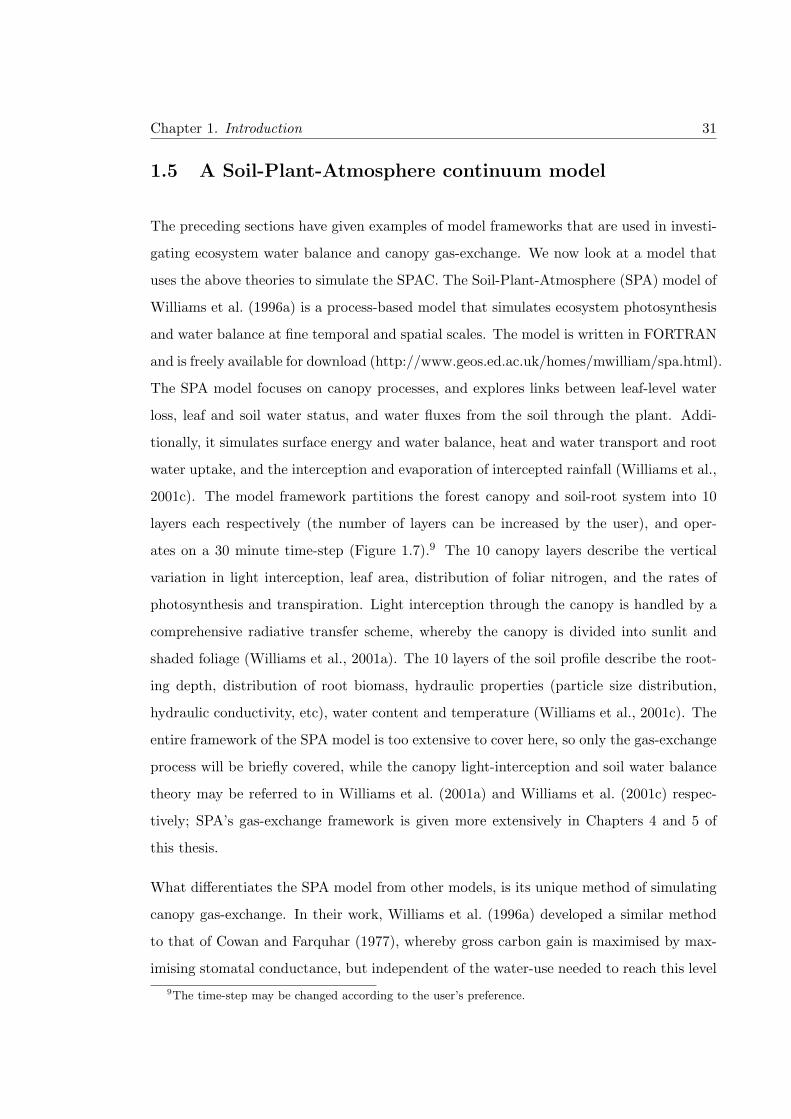
Chapter 1. Introduction 31
1.5 A Soil-Plant-Atmosphere continuum model
The preceding sections have given examples of model frameworks that are used in investi-
gating ecosystem water balance and canopy gas-exchange. We now look at a model that
uses the above theories to simulate the SPAC. The Soil-Plant-Atmosphere (SPA) model of
Williams et al. (1996a) is a process-based model that simulates ecosystem photosynthesis
and water balance at fine temporal and spatial scales. The model is written in FORTRAN
and is freely available for download (http://www.geos.ed.ac.uk/homes/mwilliam/spa.html).
The SPA model focuses on canopy processes, and explores links between leaf-level water
loss, leaf and soil water status, and water fluxes from the soil through the plant. Addi-
tionally, it simulates surface energy and water balance, heat and water transport and root
water uptake, and the interception and evaporation of intercepted rainfall (Williams et al.,
2001c). The model framework partitions the forest canopy and soil-root system into 10
layers each respectively (the number of layers can be increased by the user), and oper-
ates on a 30 minute time-step (Figure 1.7).9 The 10 canopy layers describe the vertical
variation in light interception, leaf area, distribution of foliar nitrogen, and the rates of
photosynthesis and transpiration. Light interception through the canopy is handled by a
comprehensive radiative transfer scheme, whereby the canopy is divided into sunlit and
shaded foliage (Williams et al., 2001a). The 10 layers of the soil profile describe the root-
ing depth, distribution of root biomass, hydraulic properties (particle size distribution,
hydraulic conductivity, etc), water content and temperature (Williams et al., 2001c). The
entire framework of the SPA model is too extensive to cover here, so only the gas-exchange
process will be briefly covered, while the canopy light-interception and soil water balance
theory may be referred to in Williams et al. (2001a) and Williams et al. (2001c) respec-
tively; SPA’s gas-exchange framework is given more extensively in Chapters 4 and 5 of
this thesis.
What differentiates the SPA model from other models, is its unique method of simulating
canopy gas-exchange. In their work, Williams et al. (1996a) developed a similar method
to that of Cowan and Farquhar (1977), whereby gross carbon gain is maximised by max-
imising stomatal conductance, but independent of the water-use needed to reach this level
9The time-step may be changed according to the user’s preference.

Chapter 1. Introduction 32
Figure 1.7: The soil-plant-atmosphere model partitions the forest canopy and below-ground root system into 10 layers each respectively. The canopy layers describes thevertical distributions in sunlit and shaded leaf area, distribution of foliar nitrogen (N),absorbed photosynthetically active radiation (APAR) and the rate of photosynthesis andtranspiration. The soil layers describe below-ground energy and water balance, as well asroot distribution and hydraulic properties, such as the initial soil water content (SWC)
and the particle size distribution (PSD) of the soil (percentage of sand and clay).
of productivity. Williams et al. (1996a) explain their model in terms of the efficiency of
carbon uptake, whereby the leaf will increase gs incrementally and thereby An, until such
a point that any further increase in gs does not result in an appreciable increase in An.
This conceptually ignores the increase in Et, such that the plant operates to spend the
extra water needed to gain that fraction more of carbon. This process may be formulated
as:
ιop =δAn
δgsc= An(gsc,t2)−An(gsc,t1) (1.47)
where ιop is the operating or efficiency point, which defines the degree of stomatal opening
of the plant under well-watered conditions. For the instance where soil water availability
becomes limiting there is a hydrological limit on the leaf water status, through Ψl, that
stops gsc reaching ιop in order to prevent xylem embolism. As gsc increases, Ψl will drop

Chapter 1. Introduction 33
due to an increase in Et, following the formulation of Equation 1.35. If Ψl falls to the
critical threshold at which xylem cavitation occurs (Ψl,min) then the stomata will shut in
order to prevent a critical failure of the hydraulic architecture. The effect of increasing gsc
on dΨl/dt is described by:
dΨ
dt=
Ψs −Ψl − EtRa,b
ClRa,b(1.48)
where Ψs is the soil water potential, Ra,b is the total below-ground resistance to water
flow and Cl is the leaf capacitance. This formulation links the gas-exchange component of
the SPA model with the hydraulic architecture and prevents excessive water loss by the
simulated canopy. Additionally, this gives an extra constraint in the optimisation such
that a plant will increase gsc incrementally while Ψl > Ψl,min.
This stomatal optimisation theory has been incorporated into the SPA model of Williams
et al. (1996a) and successfully used it to describe water and carbon relations for a number
of ecosystems such as an Amazonian rainforest (Williams et al., 1998; Fisher et al., 2006,
2007), Arctic tundra (Williams et al., 2000, 2001c, 2004), temperate ponderosa pine (Law
et al., 2000; Williams et al., 2001a,b), boreal (Hill et al., 2008), oak (Engel et al., 2002;
Hernandez-Santana et al., 2009) and an Australian Eucalypt forest (Zeppel et al., 2008a)
and tropical savanna (Chapter 4). The SPA model has also been tested by Misson et al.
(2004) against the JS and BBL models and show to perform equally well, and has been
incorporated into the global climate model (GCM), the Joint U. K. Land Environmental
Simulator (JULES) (Alton et al., 2009).
1.6 Work to be presented in this thesis
Having covered the background theory on surface evaporation and the exchange of water
vapour and CO2 between the atmosphere and the canopy, a set of questions are raised
which this thesis will attempt to address. These questions have been developed from some
of the common issues of modelling water and carbon fluxes from a forest canopy. The
first issue is whether a simple model (as opposed to a highly complex one) can be used to
determine canopy water fluxes without the need for a large number of inputs and detailed

Chapter 1. Introduction 34
descriptions of a site. The second issue is, given a highly complex LSM such as the SPA
model, how is it limited in its application to some ecosystems such as tropical savannas.
Additionally, is the modelled description of leaf gas-exchange in the SPA model correct?
Below are listed the four questions that encompass this thesis, as well as a description on
how each chapter will attempt to address these questions.
Question 1:
“Can water fluxes from a canopy be estimated using a simple empirical model
without the need for canopy conductance?”
The current and ongoing issue with using the PM equation is that it requires a formulation
of gc in order to derive an estimate of canopy water-use (Ec). Although the JS and TD
models offer a means of estimating gc and have been highly successful in their own right,
they still require specific calibration to site-derived data in order to be used. Chapter 2 will
therefore describe the conceptualisation of a simple empirical model of Ec that removes the
need for gc as an input. This model, a modified Jarvis-Stewart (MJS) model, will follow
a Jarvis-type structure, whereby a measure of the maximum rate of canopy water-use is
proportionally modified by a set of empirical relationships; these relationship being based
on the multivariate response of Ec to Rs, Dv and θs. The performance of this model will be
compared against the PM equation and a statistical benchmark created using an artificial
neural network (ANN).
Question 2:
“Can a simple empirical model of canopy water-use be applied across multiple
sites without the need for site-specific calibration?”
Following on from Question 1, Chapter 3 will look at the applicability of the MJS model
across five disparate Australian woodland sites. This will involve a calibration of the
model to each site individually and then to all sites simultaneously, with the aim being to
determine a set of site-specific and site-average parameters that can be used in the model

Chapter 1. Introduction 35
to derive estimates of Ec at each site. The idea of this approach is to see how sensitive the
model is to variation in the value of the model parameters and whether or not an set of
site-average parameters can give reasonable predictions of site Ec. If a set of site-average
parameters do not result in a decline in model performance, then this will remove the need
to calibrate the model at each site and reduce the amount of required information to run
the model.
Question 3:
“Can the Soil-Plant-Atmosphere model be used replicate canopy gas-exchange
for a Australian tropical savanna?”
A distinct limitation of the SPA model is that it only considers C3 photosynthetic processes
(Appendix A). Although this is not a problem for many temperate landscapes, tropical
savannas (an important global biome) are dominated by C4 grasses that make significant
contributions to ecosystem biomass (Hutley et al., 2000; Chen et al., 2002, 2003; Kanniah
et al., 2010a). Chapter 4, details the incorporation of C4 photosynthesis into the SPA
model necessary in extending its applicability towards tropical savannas. The reasoning
behind using savannas as the test-bed for this exercise is as that they are a dominant
ecosystem globally and consequently they influence regional and global carbon budgets
extensively. Despite this, savannas have not been extensively modelled in the literature,
and there is a major gap in savanna research; especially as most models do not include a C4
photosynthesis model. This will involve the testing of two C4 photosynthesis sub-models
as well as the parameterisation of the SPA model to a savanna site. The consequence of
this will provide a way of investigating the contribution of C4 vegetation to total savanna
ET and gross primary productivity (GPP). Additionally, the question of what drives the
seasonality of ET and GPP in a savanna will be investigated.
Question 4:
“Can the leaf gas-exchange process in the SPA model be improved so as to
maximise carbon gain while simultaneously minimising water loss from the leaf

Chapter 1. Introduction 36
following the Cowan and Farquhar optimality hypothesis?”
The current framework of the leaf gas-exchange process in SPA works towards maximis-
ing An by increasing gs; that is, gs is increased until there is no appreciable increase in
An. This representation of leaf gas-exchange, causes the SPA model to transpire copious
amounts of water in order to gain an infinitesimal amount of carbon. This process ignores
the “optimality hypothesis” of Cowan and Farquhar (1977) who state that the leaf must
maintain some balance between the water lost from the leaf and the carbon gained by the
leaf. Chapter 5, describes a possible solution to this problem by introducing the limitation
of Et on gas-exchange into Equation 1.47 following the optimality hypothesis (Cowan and
Farquhar, 1977). This modification to the SPA model will be tested over a 30 day drying
period, in order to observe any benefits of this modification and to highlight the effects of
soil drying on leaf gas-exchange. The goal of this chapter will be to determine whether or
not the SPA model responds correctly to drought.

Chapter 2
Comparing the Penman-Monteith
equation and a modified
Jarvis-Stewart model with an
artificial neural network to
estimate stand-scale transpiration
The work presented in this chapter was first conceptualised, peer reviewed and published in
a special edition of Plant and Soil, volume 305 (2008), pages 35-47. This work was then
further extended, peer reviewed and published in the Journal of Hydrology, volume 373
(2009), pages 256-266. I acknowledge that the work presented here is my own, and that
any involvement by other persons has been duly acknowledged in the text. The publication
Whitley et al. (2009) has therefore been incorporated almost verbatim as a chapter in this
thesis. Specifically, I acknowledge that all the field data used in this chapter were collected
by Zeppel et al. as described in Zeppel et al. (2004)
37
Chapter 2. Comparing the Penman-Monteith equation and a modified Jarvis-Stewartmodel with an artificial neural network to estimate stand-scale transpiration 38
2.1 Introduction
Measuring tree water-use is an important step in determining the water balance of woody
landscapes (Komatsu et al., 2006a; Wullschleger and Hanson, 2006; Rollenbeck and Di-
eter, 2007; Simonin et al., 2007) and determining landscape water balances is important to
forestry and mining industries, to water and landscape management agencies and the land-
atmosphere modelling community. Whilst estimating tree water-use can be undertaken
using sapflow technologies (O’Grady et al., 1999; O’Grady, 2006), such measurements are
made at the scale of individual trees, usually over relatively short time frames (days and
weeks) and typically only during the growing season (Wullschleger et al., 1998; Lundbald
and Lindroth, 2002). However, to obtain the required annual estimates of stand transpi-
ration rates, up-scaling spatially and temporally is required; even when there is continual
monitoring of a few trees at a site. Whilst eddy covariance (EC) measurements of stand
water-use give integrated measures of vegetation water-use (Hutley et al., 2000; Eamus
et al., 2001; Ewers et al., 2007), EC is expensive, technically challenging and requires
large, flat homogenous landscapes. Key end-users who require annual estimates of vege-
tation water-use (including mine-site managers, catchment management authorities and
water resource managers) require a methodology that is sufficiently robust to be useful,
but not too resource (time, equipment, data) intensive and one that is applicable to un-
even terrain or small plots. An application of a simplified model of vegetation water-use,
as applied to management of groundwater dependent ecosystems, can be found in Howe
et al. (2005).
Water flux through trees is a principal pathway for the discharge of soil water. Conse-
quently, to determine the water budget of woody landscapes, tree canopy water fluxes must
be known, either through direct measurement or through modelling (Komatsu et al., 2006a;
Wullschleger and Hanson, 2006; Rollenbeck and Dieter, 2007; Simonin et al., 2007). Stom-
atal conductance (gs), solar radiation (Rs), vapour pressure deficit (Dv) and soil moisture
content (θs) are the major determinants of tree water fluxes (Jarvis and McNaughton,
1986; Wullschleger et al., 2001; Zeppel, 2006; Zeppel and Eamus, 2008; Zeppel et al.,
2008b) and seasonal variations in these three abiotic variables cause seasonal variation
of canopy conductance (gc) and canopy transpiration (Ec) (Harris et al., 2004; Komatsu

Chapter 2. Comparing the Penman-Monteith equation and a modified Jarvis-Stewartmodel with an artificial neural network to estimate stand-scale transpiration 39
et al., 2006b). Measuring seasonal variations of these abiotic variables and parameterising
their impact is important for quantifying intra-annual variation in gc and Ec.
The Penman-Monteith (PM) equation (Monteith, 1965) is commonly used to estimate
evapotranspiration of crops (Yunusa et al., 2000; Lu et al., 2003) and forests (Gash et al.,
1989; Kosugi et al., 2007; Zeppel and Eamus, 2008). In the past two decades the PM equa-
tion has been simplified by assuming forest canopies are highly coupled to the atmosphere
(Granier et al., 1996b; Whitehead, 1998; Granier et al., 2000; Ewers et al., 2007). The base
assumption is that transpiration (Et) is controlled by stomatal resistance to water flow
(rs; the inverse of gs) in response to meteorological forcing and assuming that atmospheric
resistance (ra) in the soil-plant-atmosphere pathway is very low (rs � ra). The rate of
water loss from the surface of a leaf is calculated as:
Et = gs(es − ea)
= gsDv (2.1)
where es and ea are the vapour pressures at saturation and in the air, such that Dv =
es − ea. Water lost from the leaf, can then be scaled up to the water lost from the surface
of the forest canopy by multiplying the right-hand side of Equation 2.1 by the leaf area
index (LAI) (Whitehead, 1998), such that:
Ec = LAI · gsDv
= gcDv (2.2)
The regulation of gc and Ec has received extensive investigation (Jarvis, 1976; Stewart,
1988; Granier and Loustau, 1994; Harris et al., 2004; Komatsu et al., 2006b). Such studies
use measured values of sap-flow or EC and an inversion of the PM equation to derive
measurements of gc. In most applications of the PM equation, a Jarvis-type model (Jarvis,
1976; Stewart, 1988) is used to quantify gc via set of seasonal response terms, describing
the functional relationships relating to Rs, Dv and θ. This approach has been applied
over the past 30 years to various stands comprised of different species, such as temperate
poplar, maritime pine, oak, spruce and pine forests (Gash et al., 1989; Dolman et al., 1991;

Chapter 2. Comparing the Penman-Monteith equation and a modified Jarvis-Stewartmodel with an artificial neural network to estimate stand-scale transpiration 40
Ogink-Hendriks, 1995; Wright et al., 1995; Zhang et al., 1997; Lagergren and Lindroth,
2002; Sommer et al., 2002), Amazonian pastures and rainforests (Harris et al., 2004) and
Japanese conifer forests (Komatsu et al., 2006a,b). Parameterisation of a Jarvis-type
model over an annual cycle for Australian native woodlands and forests has not yet been
conducted. Responses of gs and Et to Dv have been investigated for northern Australian
savannas by Thomas and Eamus (1999); Thomas et al. (2000) and Eamus and Shanahan
(2002) and soil moisture responses of Ec and gc have been investigated (Hutley et al., 2001;
Zeppel and Eamus, 2008; Zeppel et al., 2008b).
Jarvis-type models have been used extensively because of their simplicity and they allow
calculation of gc as a function of meteorological variables and soil water availability. How-
ever, one problem in applying Jarvis-type models is the requirement for a large degree of
spatial and temporal replication in gc and subsequent use of the PM equation in order to
calculate Ec. Consequently, the frequent problem of having to quantify gc poses difficulties
in readily applying the PM equation. Furthermore, the PM equation is known to predict
Ec poorly under limiting soil moisture conditions and it may correlate with observations
best when Ec is large (David et al., 1997; Rana et al., 2005). In order to overcome this
problem, the work contained herein describes a relatively simple empirical model whereby
scaled estimates of Ec can be made from readily available meteorological measurements
(Rs, Dv and θs) without the need to measure gc. This model is conceptualised on the em-
pirical framework of Jarvis (1976) and Stewart (1988) and in reference to this it has been
coined as the modified Jarvis-Stewart (MJS) model. Additionally, this model is compared
against the PM equation, with the performance of both models (MJS and PM) being
tested against a statistical benchmark, which has been created using an artificial neural
network (ANN). Finally, the results are compared with those found in previous studies to
show the spatial variability of models parameterised over different sites and ecosystems.

Chapter 2. Comparing the Penman-Monteith equation and a modified Jarvis-Stewartmodel with an artificial neural network to estimate stand-scale transpiration 41
2.2 Methods
2.2.1 Site description
A remnant open woodland site located approximately 70 km south of Tamworth, in north-
western NSW (31.5◦S, 150.7◦E, elevation 390 m), was used in this study. A full description
of the site is provided in Zeppel et al. (2004) and Zeppel and Eamus (2008). In summary,
the average height of the trees was 15 m and is dominated by Eucalyptus crebra and
Callitris glaucophylla. These two species contributed approximately 75 % of the tree
basal area at the site. Total tree basal area was 23.8 ± 3.4 m2 ha−1. The eucalypts
had a lower density than the Callitris (42 stems ha−1 compared to 212 stem ha−1) but
contributed most (approximately 75 %) to the basal area of the two species combined
because its average diameter was much larger than that of the Callitris. The understorey
was dominated by grasses, predominantly Stipa and Aristada species. Soils at the site were
shallow with well-drained acid lithic bleached earthy sands (Banks, 1998) with occasional
exposed sandstone.
Incoming solar radiation and wet and dry bulb temperature were measured at hourly
intervals at a weather station located in a cleared pasture (> 4 ha) approximately 100 m
from the remnant woodland. Wind speed was measured with a cup anemometer situated
about 3 m above the canopy and soil moisture was measured with Theta Probes (Delta-T
Devices, UK) at 50 cm depth at two locations. LAI was measured at seven locations in
the woodland, as previously described (Zeppel, 2006) using a Li-Cor 2000 Plant Canopy
Analyser, four times during the year of study (2004). LAI ranged from 0.9 to 1.0 on these
four occasions (data not shown).
2.2.2 Water use by individual trees
The rate of water-use by individual trees (L d−1) was measured by Zeppel et al. (2004) at
15 minute intervals using sap-flow sensors (model SF100, Greenspan Technology, Pty Ltd,
Warwick, Australia). For each species 10-12 trees were chosen to sample the full range
of tree sizes and each tree was instrumented with 4 sensors. Sensors were stratified with

Chapter 2. Comparing the Penman-Monteith equation and a modified Jarvis-Stewartmodel with an artificial neural network to estimate stand-scale transpiration 42
depth (at 1/3 and 2/3 of the depth) through the sapwood (Medhurst et al., 2002; Zeppel
et al., 2004). sap-flows were corrected for wound effects, sapwood area, radial variability
in flow and volumetric fractions of water and wood (Zeppel et al., 2004). Wound width
was measured for both sensor sets in each of seven trees of both species at the end of the
sampling period, following the method of O’Grady et al. (1999). A wound width of 2.5
mm for C. glaucophylla and 3.7 mm for E. crebra was used to correct velocity estimates.
Basal area and diameter at breast height (DBH) of all trees were measured in 7 replicate
50 m x 50 m plots (Zeppel et al., 2004).
2.2.3 Scaling to stand transpiration
Scaling from individual trees to stand transpiration was done by multiplying the average
hourly sap velocity (Vsap) by the sapwood area per unit ground area (Asap); further de-
tails of this can be found in Zeppel et al. (2004) and Whitley et al. (2008). AS plot was
calculated from measurements of sapwood depth for both tree species and from plot-level
measurements of the stand. Each 24 hour period was summed to give the daily sap flux
(cm3 plot−1 d−1). The water-use (cm3 H2O plot−1 d−1) of each plot (with an area of 2500
m2) was converted to the stand scale (mm3 H2O mm−2 ground area [GA] d−1). The DBH
of all trees in 7 replicate plots was measured and therefore there were 7 estimates of stand
water-use (cm3 sapflux cm−2 GA d−1) for each day. The mean and standard error of all
7 plots, for each day, was then estimated, and converted from cm3 H2O cm−2 GA d−1 to
yield stand water-use (Ec, mm hr−1).
2.2.4 Models
The goals for this analysis were threefold. First, to parameterise two transpiration models
in order to derive a set of seasonal response terms describing the responses of Ec and
gc to changes in their driving environmental variables. Second, to compare estimates
of modelled Ec made via an empirical model (Whitley et al., 2008) with those made
from the PM equation. Finally, to quantify the performance of these models statistically
by comparing model outputs, against that of an artificial neural network (ANN). I now
outline the two models used in this study and then describe the ANN applied to the data.

Chapter 2. Comparing the Penman-Monteith equation and a modified Jarvis-Stewartmodel with an artificial neural network to estimate stand-scale transpiration 43
2.2.4.1 The Penman-Monteith model
The PM equation calculates the latent energy lost from the canopy as:
λEc =ΔRn + ρacpDvgaΔ+ γ(1 + ga/gc)
(2.3)
where Δ is the slope of the relationship between the saturation vapour pressure and tem-
perature (kPa ◦C−1), ρa is the air density (1.204 kg m−3 @ 20◦C ), cp is the specific heat
of air (1.013 MJ kg−1 ◦C−1), γ is the psychometric constant (0.066 kPa ◦C−1), λ is the
latent heat of vaporisation (2.39 MJ kg−1), Rn is the net radiation above the forest canopy
(MJ m−2 hr−1; converted from W m−2) and is calculated from Rs using an expression
from Eagleson (2002) given as:
Rn = Rs(1− α)− 57.65 (2.4)
where α is the albedo of the earth’s surface (≈ 0.2) and 57.65 represents a constant level
of longwave radiation (W m−2). Lastly, ga is the aerodynamic conductance (m s−1) and
is estimated from:
ga =(1 + 0.54U)
4.72 ln(Z/Z0)2(2.5)
where U is the wind speed above the canopy (m s−1), Z is the height of the forest canopy
(m) and Z0 is the roughness length for the forest type (1.95 m for this forest type; from
Zeppel et al. (2008b)). Using a Jarvis-type model, gc is expressed empirically as:
gc = gcmaxf1(Rs)f2(Dv)f3(θ) (2.6)
where the functions fi are a set of scaling terms that reduce gcmax in response to changes
in Rs, Dv and θ; scaling from leaf to canopy level and vice versa is achieved through the
LAI term, incorporated via the gcmax parameter such that gcmax = LAI gsmax. The func-
tions fi take on values between 0 and 1, proportionally modifying gcmax to give modelled
estimates of gc1. The functional forms for climatic forcing on stomatal aperture used in
1It is assumed that the responses to each driving variable are independent (Jarvis, 1976).

Chapter 2. Comparing the Penman-Monteith equation and a modified Jarvis-Stewartmodel with an artificial neural network to estimate stand-scale transpiration 44
this study are taken from Harris et al. (2004), and are expressed as:
f1(Rs) =
(Rs
1000
)(1000 + k1Rs + k1
)(2.7)
f2(Dv) = exp(−k2Dv) (2.8)
f3(θ) = min
{1,
θ − θwθc − θw
}(2.9)
where the parameters gcmax, k1, k2, θw and θc are free parameters determined through
least-squares optimisation. Equation 2.7 describes the asymptotic response of increasing
Rs, with saturation occurring at approximately 1000 W m−2 and k1 (W m−2) describing
the curvature of the relationship. Hyperbolic saturating functions describing Rs have been
applied extensively at leaf, tree and canopy scales for conductance (Kelliher et al., 1993;
Granier et al., 2000) and for tree water-use (Komatsu et al., 2006b). Equation 2.8 describes
the exponential decay of gc due to increasingDv, where k2 (kPa) describes the rate of decay.
Equation 2.9 shows the soil moisture response to be a piece-wise relationship, where θw
and θc (m3 m−3) denote the points of inflection in the relationship and can loosely be
termed as the wilting and critical points respectively.
In order to parameterise Equation 2.6, an inversion of the PM equation was solved in order
to derive measurements for gc (mm s−1) and is given as:
gc =γλEcga
ΔRn + tcρacpDvga − λEc(Δ + γ)(2.10)
The parameters gcmax, k1, k2, θw and θc are determined by minimising the difference
between Equations 2.6 and 2.10, using a nonlinear optimisation method (explained later in
this chapter). The optimised parameter values are then used in Equation 2.6 to determine
modelled values of gc which are then inserted into Equation 2.10 in order to derive modelled
estimates of Ec.

Chapter 2. Comparing the Penman-Monteith equation and a modified Jarvis-Stewartmodel with an artificial neural network to estimate stand-scale transpiration 45
2.2.4.2 The modified Jarvis-Stewart model
Following the formulation and theory given by Equation 2.2, Ec can be modelled empiri-
cally using a Jarvis-type approach that can circumvent the need for gc as a model input.
For a well-coupled forest, where water lost from the leaf is controlled by stomatal aperture
in response to meteorological changes, the mass transfer of water can be equated to follow
an Ohm’s law analogue, such that water lost from the canopy surface can be described by
the equation:
Ec = gcDv (2.11)
Following that, gc is primarily controlled by variations in Rs, Dv and θ, and Equation 2.6
can be inserted into Equation 2.11, such that:
Ec = gcmaxf1(Rs)f2(Dv)f3(θ) ·Dv (2.12)
and noting that:
Ecmax = gcmaxDv (2.13)
it follows that water lost from the surface of the forest canopy can be described empirically
as:
Ec = Ecmaxf1(Rs)f2(Dv)f3(θ) (2.14)
where once again the functions fi describe a set of modifiers that proportionally modify
Ecmax in response to changes in Rs, Dv and θ. The functional responses of Ec to variations
in Rs and θ are the same responses as described by Equations 2.7 and 2.9. However, the
response of Ec to increasing Dv is different as it includes the response of stomata shutting
down at highDv to maintain turgor and conserving water supply. This is generally referred
to as the three-phase response (Monteith, 1995). Therefore, a new function is defined to
explain the variation of Ec with Dv and is given as:
f2(Dv) = k2Dv exp(−k3Dv) (2.15)

Chapter 2. Comparing the Penman-Monteith equation and a modified Jarvis-Stewartmodel with an artificial neural network to estimate stand-scale transpiration 46
where, the parameters k2 and k3 describe the rate of change at low and high atmospheric
demand. This is a new term and follows the shape of a Bolztmann distribution function.
Examination of Equation 2.15 shows that it replicates the three-phase response of tran-
spiration to variation in gs as Dv is increases from low to high values. Monteith (1995)
has reviewed this topic and Eamus and Shanahan (2002) and Thomas and Eamus (1999)
provide experimental and model verification. However, this is not normalised as Equations
2.7, 2.8 and 2.9 are, and some care is needed optimising Equation 2.14. Hourly estimates
of modelled Ec (mm hr−1) were determined from functions fi.
The formulation given in Equation 2.14 is functionally equivalent to the PM equation, yet
is much simpler to fit, requires fewer measurements and specifically removes gc as a model
input, a problem concurrent in all studies that use the PM equation (Ewers and Oren,
2000; Lu et al., 2003; Pataki and Oren, 2003); but retains it structurally within the model
through the parameter Ecmax. Additionally, Equation 2.14 Is structurally equivalent to
Equation 2.3 assuming that the forest canopy is highly coupled to the atmosphere, such
that gc � ga, and so Equation 2.3 reduces to:
λEc =ρacpDvgc
γ
Ec =ρacpλγ
· gcDv (2.16)
Expressing Ec as function of Rs, Dv and θ in this way, follows the model structure defined
by Jarvis (1976) and Stewart (1988), and so this empirical equation has been coined (in
the context of this study) as the modified Jarvis-Stewart (MJS) model.
2.2.4.3 Model parameterisation
Both models were parameterised from experimental (measured) data using a genetic algo-
rithm and weighted least squares (WLS). A weighting term (σi) was incorporated to better
quantify the distribution of error in the measurements and hence ensure the optimised free
parameters were closer to maximum likelihood. The parameters Ecmax, gcmax, k1, k2, θw
and θc are the optimised free parameters that represent response constants in the JS mod-
els. A multivariate optimisation for Equations 2.6 and 2.14 was done by minimising the

Chapter 2. Comparing the Penman-Monteith equation and a modified Jarvis-Stewartmodel with an artificial neural network to estimate stand-scale transpiration 47
weighted sum of the square of residuals (WSSR). Given that the model parameters are set
at some arbitrary starting values, we express the WSSR as:
χ2min =
N∑i=1
(Yi − f(Xi, β)
σi
)2
(2.17)
where
σi = b Yi (2.18)
and Yi is the ith experimental value, f is the model equation, where Xi and β being the
ith model variables and parameters respectively, σi is the ith standard deviation and N
is the number of data points. It is assumed that the heteroscedasticity is explained by
Equation 2.18; expressing the standard deviation to be proportional to the experimental
data Yi, multiplied by an error constant of proportionality b (Kirkup et al., 2004). In
order to specify whether σi is normally distributed, it is assumed that the residuals are a
surrogate for σi such that σi = Yi − Yi. For this study, random measurement error (σi)
has been assumed to be normally distributed and heteroscedastic based on observations
of the weighted residuals. The parameters values necessary to run the PM equation can
therefore be found by inserting Equations 2.6 and 2.10 into 2.17:
χ2gc =
N∑i=1
⎛⎝ γλEc,iga,i
ΔRn,i+tcρacpDv,iga,i−λEc,i(Δ+γ) − gcmaxf1(Rs,i)f2(Dv,i)f3(θi)
bγλEc,iga,i
ΔRn,i+tcρacpDv,iga,i−λEc,i(Δ+γ)
⎞⎠2
(2.19)
and the parameter values necessary to run the MJS model are found similarly by inserting
Equation 2.14 into 2.17:
χ2Ec
=N∑i=1
(Ec,i − Ecmaxf1(Rs,i)f2(Dv,i)f3(θi)
bEc,i
)2
(2.20)
The two formulations above, show the difficulties in optimisation that are commonly ex-
perienced when using a least squares criterion at large dimensionalities. As the problem
moves from linear to non-linear, the parameter space very quickly becomes increasingly
populated by local minima and is therefore increasingly difficult to find the global min-
imum pertaining to the correct parameter values. Where local minima occur over the

Chapter 2. Comparing the Penman-Monteith equation and a modified Jarvis-Stewartmodel with an artificial neural network to estimate stand-scale transpiration 48
large parameter space, early convergence of the solution is likely to occur, hampering the
optimisation. To overcome these problems, a genetic algorithm was incorporated instead
of the traditional Levenberg-Marquardt or Gauss-Newton algorithms. Unlike the gradient
descent methods, a genetic algorithm is able to cover the entire parameter space with a
large set of possible solutions. These solutions evolve and undergo a simulated process of
natural selection until the best solution and hence the global minima equating to parame-
ter values that are maximum likelihood, is found. A more detailed explanation of genetic
algorithms and their design can be found in (Goldberg, 1989). For this study we used a
pre-built genetic algorithm package in the Mathematica c© software called Differential Evo-
lution. The cross probability (probability of mating) was set to 50%, while population size
was set automatically by the algorithm and run for 100,000 iterations to give an adequate
amount of generations to find the global maxima.
2.2.4.4 Artificial neural network
In order to test the MJS model and PM equation against some form of statistical bench-
mark, an ANN was used as a comparator (Kohonen, 1989; Hsu et al., 2002; Abramowitz,
2005). A multivariate ANN procedure called a Self-Organising Linear Output map (SOLO)
developed by Hsu et al. (2002) was used for this study to create this statistical benchmark
and Figure 2.1 shows a diagram of this process. SOLO learns the relationship between
inputs and outputs through the use of a training data set. Input information (Rs, Dv and
θ) is classified in a Self Organising Feature Map (SOFM) (Kohonen, 1989). The SOFM
is built by grouping parcels of input information into groups or nodes and are assigned a
weighting term, where each weighting term corresponds to a specific pattern of input data.
This SOFM is then connected to a prediction map, which is constructed by a multiple lin-
ear regression between input information (three abiotic drivers) and output information
(canopy water-use). Regression parameters are determined from each node and are se-
lected according to the supplied input data at a specific time-step; that is, a set of Rs, Dv
and θ values will correspond to a specific Ec value. Thus, SOLO produces a piece-wise
linear reconstruction of any functional relationship between these two groups (inputs and
outputs) of variables (Abramowitz et al., 2009). The limitation of this process is that
it requires a large amount of data (which determines the number of nodes) to construct

Chapter 2. Comparing the Penman-Monteith equation and a modified Jarvis-Stewartmodel with an artificial neural network to estimate stand-scale transpiration 49
significant relationships so as to give an effective statistical reconstruction of the desired
output. Although this is the basic idea behind the SOLO ANN, the theory behind this
process is given in greater detail in Hsu et al. (2002).
Figure 2.1: Diagram of the self-organising linear optimisation (SOLO) artificial neuralnetwork (ANN). The grey square denotes the self-organising feature map (SOFM) whichcontain nodes (red circles) of grouped input information, i.e. solar radiation, vapour pres-sure deficit and soil moisture content (yellow circles; x1, x2 . . . xn), where the data con-tained in each node are linearly related. Nodes in the SOFM network are compared withmeasurements of the desired output, i.e. canopy transpiration (green circles; y1, y2 . . . yn)through a multivariate linear regression in the linear mapping network. This allows func-tional relationships between the input and output information to be developed. Further
input data can then be fed into SOLO to reconstruct the desired output (z1).
The ANN is a pure statistically-based response to the meteorological forcing on a per time
step basis (Abramowitz, 2005). The purpose of comparing a conceptual model against an

Chapter 2. Comparing the Penman-Monteith equation and a modified Jarvis-Stewartmodel with an artificial neural network to estimate stand-scale transpiration 50
ANN output must be clearly understood. The ANN will always outperform mechanistic,
conceptual models because it effectively has up an infinite number (theoretically) of op-
timised parameters, whereas most conventional models have at most 10 to 30. A direct
comparison is therefore inappropriate. However, the ANN informs us about the informa-
tion content of the data-set. That is, it indicates whether a model is performing badly
because it fails to capture underlying relationships in the data, or whether it is performing
badly because the dataset is too noisy. Thus, it offers a statistical evaluation of model
performance.
In this study, a statistical benchmark was created using the SOLO ANN, where the three
meteorological drivers (Rs, Dv and θ) containing 2616 data points (per variable) were used
to construct a 5 x 5 SOFM. The size of the SOFM was kept small due to the low number
of data points. The 5 x 5 SOFM was then used in SOLO along with Ec data in a training
process, which was then subsequently used to simulate purely statistical predictions of Ec.
2.2.4.5 Filtering the data set
Sap flow data were filtered to avoid division by zero errors by including data only between
0900 h and 1600 h. This exclude hours when solar radiation was zero. To avoid wet-canopy
conditions, days with rainfall events were also excluded. This filtered data-set was used to
define the boundary conditions for Equations 2.7, 2.8, 2.9 and 2.15. To avoid circularity
(using the same data to both parameterise the model and to compare with model outputs),
the total 109 day data set spanning the year containing measurements from Jan-Feb, Jun-
Jul and Aug-Sep, were partitioned into two separate data sets of alternate days. The first
set (days 1, 3, 5 .) was used to optimise the seasonal response parameters, and the second
set (days 2, 4, 6 .) was used to validate the model. No systematic patterns were evident
in the data and there was no change in model outputs when allocation of each half of the
data set to either optimisation or validation was reversed. However, it is noted that this
does not result in two truly independent data-sets as, for example, rainfall on one day will
affect Ec on the following day.

Chapter 2. Comparing the Penman-Monteith equation and a modified Jarvis-Stewartmodel with an artificial neural network to estimate stand-scale transpiration 51
2.3 Results
2.3.1 Meteorological and sap-flow data
Maximum daily Rs ranged from 100 to almost 1400 W m−2 in summer and from 100
to 800 W m−2 in winter whilst the maximum daily Dv ranged between 0.5 to 7.0 kPa in
summer and 0.1 to 1.6 kPa in winter (Figure 2.2a). The Liverpool Plains are characterised
by summer dominant rainfall and a drier winter and this was evident during the study
period, when there were 19 rain events during January and late February and 6 smaller
events in July, August and September (Figure 2.2b). Summer maximum daily soil moisture
content reached 13.9 % after two consecutive rain events during January, with subsequent
decreases in Ec resulting from a gradual decline in θ to a minimum of 9 % (Figure 2.2b).
During winter maximum daily θ reached a maximum of 10.8 % after a small 2 day rain
event and a minimum of 9.4 % (Figure 2.2b). Mean daily Ec measured with the sap-flow
sensors (scaled by sapwood area) varied up to 8-fold on consecutive days, with a range
of from 0.09 mm d−1 during a rainy day (24th Feb) up to approximately 2.8 mm d−1
(28th Feb) on a rain-free day in the summer (Figure 2.2c). During winter, Ec varied
between no measurable transpiration (Ec << 0.01 mm d−1) on a rainy day (11th Jul) up
to 2.08 mm d−1 on a rain-free day (28th Jul). Declining Ec between the 4th Feb and 22nd
Feb was associated with declining θ, whilst large increases in Ec occurred after the 13th
Jan and after 24th Feb following large rain events and hence soil recharge. An increase
in soil moisture was evident from the 1st Aug, and was associated with an increase in
stand water-use. The three largest rainfall events during the summer period increased soil
moisture at 60 cm depth, whereas during winter most rainfall events had little effect on
soil moisture at 60 cm depth (Figure 2.2 b).
2.3.2 Modelled stand water-use
The five parameters in Equation 2.6 and six parameters in Equation 2.14 were opti-
mised by minimising the WSSR by using the Differential Evolution genetic algorithm
in Mathematica c©. Results from the genetic algorithm produced a set of maximum like-
lihood parameters that best describe seasonal responses. Figure 2.3 a, b, c shows the

Chapter 2. Comparing the Penman-Monteith equation and a modified Jarvis-Stewartmodel with an artificial neural network to estimate stand-scale transpiration 52
Figure 2.2: Day-to-day variation in canopy transpiration and its driving variables atParinga. Data shown is the (a) daily maximum incident solar radiation (Rs), daily max-imum vapour pressure deficit (Dv), (b) total soil water content to a depth of 60 cm (θs),daily rainfall and (c) total daily stand transpiration (Ec) for the periods of (left) January
- February and (right) July - September 2004.
relationships between Ec and the driving variables Rs, Dv and θ and Figure 2.3 d, e, f
shows the relationships of gc against the same driving variables. Generally the functional
forms fit well to the boundary regions described by the data, except for the response of
Ec to Dv for the winter (Figure 2.3b). The residuals between measured and modelled
data (Figure 2.4) reveal a minor heteroscedasticity, as evident by the slight pattern of the
residuals. In order to properly account for this heterscedascticity, we used a weighting
term (Equation 2.18). Using this weighting term explained the random errors (ε) in the
measurements to be normally distributed, with the 68% confidence interval being within
±1 standard deviation (data not shown). Table 2.1 contains the best estimates of the
parameters in Equations 2.7, 2.8, 2.9 and 2.15 along with their respective standard errors.
All parameter values were found to be statistically significant (P < 0.05).

Chapter 2. Comparing the Penman-Monteith equation and a modified Jarvis-Stewartmodel with an artificial neural network to estimate stand-scale transpiration 53
Figure 2.3: The functional dependencies based on the optimised parameters of canopytranspiration (Ec) on: (a) solar radiation (Rs), (b) vapour pressure deficit (Dv) and (c)soil water content at a depth of 60 cm (θ); and canopy conductance (gc) on (d) Rs, (e) Dv
and (f) θs. Relationships are given by white circles for summer (�) and black diamondsfor winter (p). The red lines are the functional response curves (f1...3) that describenon-limiting relationships between the quantities of Ec and gc, and its environmental
drivers.
The seasonal response parameters relating to gc were used in Equation 2.6, which in turn
was used in the PM equation (Equation 2.3) to give estimates of canopy water-use (EPMc ).
The seasonal response parameters relating to Ec, were used in MJS model (Equation 2.14)
to derive estimates of canopy water-use (EJSc ). Figure 2.5 shows a comparison of Ec
estimates from both the PM equation and MJS model, against scaled measurements (EObsc )
and predictions from an ANN (EANc ) over the January-February summer period and July-
September winter period. There was a slight under-prediction of EObsc using both models,
from the 17th-23rd Jan and 25th-29th Feb, which coincides with prior large rain events.
Under-prediction of EObsc was observed throughout the winter period but it was only

Chapter 2. Comparing the Penman-Monteith equation and a modified Jarvis-Stewartmodel with an artificial neural network to estimate stand-scale transpiration 54
Figure 2.4: Weighted residuals (measured − modelled) for (a) the Penman-Monteith(PM) equation and (b) their distribution of error, and the weighted residuals for (c) themodified Jarvis-Stewart (MJS) model and (d) their distribution of error. The dashed linesshow the regions for which the residuals fall between ±1 standard deviations, representa-tive of the 68% confidence region. Both models conform to the assumption of a normally
distributed error about a mean 0 and standard deviation 1.
occasionally seen in the summer. This under-prediction in both cases affects the total
daily sums of Ec from both models. The ANN shows a night-time bias in its fitting,
resulting in predictions of night-time Ec during both summer and winter periods which
are not always measured by the sap-flow sensors, especially in winter. The ANN was unable
to account for night-time Ec from the 27th-31st July. Points of failure in the fitting seem
to be replicated across both models and the ANN. A comparison of both models shows
that EJSc is much closer to the ANN in terms of explaining observed variations in Ec.
To allow a more detailed comparison amongst the ANN and model outputs, changes in

Chapter 2. Comparing the Penman-Monteith equation and a modified Jarvis-Stewartmodel with an artificial neural network to estimate stand-scale transpiration 55
Figure 2.5: Canopy transpiration (Ec) measured with sapflow sensors (data points) andestimated Ec from the modified Jarvis-Stewart (MJS) (blue line), the Penman-Monteith(PM) equation (red line), and the statistical benchmark created using an artificial neuralnetwork (ANN; gold line) over the sampling periods in (a) January, (b) February, (c) July
and (d) September 2004.

Chapter 2. Comparing the Penman-Monteith equation and a modified Jarvis-Stewartmodel with an artificial neural network to estimate stand-scale transpiration 56
Table 2.1: Parameter estimations resulting from an optimisation of the modified Jarvis-Stewart (MJS) model and Penman-Monteith (PM) equations using a genetic algorithm.Parameters defined here are both maximum reference values for maximum canopy con-ductance (gcmax; m s−1) and canopy transpiration (Ecmax; mm hr−1), environmentalfunctional dependencies on solar radiation (Rs), (k1; W m−2), vapour pressure deficit(Dv), (k2 and k3; kPa), and soil water content (θs) at wilting (θw), and critical points(θc; mm2 mm−2), the constant of proportionality associated with error (b) and explainedvariance (R2). Standard errors (S.E.) are given as a fraction of the parameter value in
brackets.
EPM EJS
Parameter Value S.E. Value S.E
gcmax/Ecmax 0.0082 (0.02) 0.267 (0.02)k1 257.99 (0.19) 200.38 (0.20)k2 1.08 (0.02) −k3 0.39 (0.03) 0.44 (0.11)θw 0.071 (0.02) 0.07θc 0.115 (0.01) 0.118 (0.01)
b 0.38 0.29R2 0.86 0.87
RMSE 0.0159 0.0042slope 0.92 0.91
intercept 0.023 0.025
hourly rates of Ec for four representative days are presented in Figure 2.6. In summer
months, the MJS and PM models represent the morning trend of increasing sap-flow
equally well but neither was able to represent the late afternoon/early evening trends in
sap-flow very accurately. On average, in summer, the MJS model either slightly (< 10%)
under-estimated or slightly over-estimated mid-day rates of Ec, whilst the PM equation
either closely matched or under-estimated by a larger margin (15%) mid-day rates of Ec.
The ANN consistently followed the changes in Ec more closely throughout the 24 hr period.
The performance of both models was less satisfactory in winter than summer (Figure 2.6).
The PM model consistently under-estimated the rate of Ec, particularly in the morning,
but over-estimated Ec in the afternoon on some days. The MJS model performed better
than the PM model in winter by a better representation of the maximum rates of Ec.
However, it failed to adequately represent the early morning increase in Ec observed in
the data. As expected the ANN closely matched the daily trends in Ec. The sap-flow

Chapter 2. Comparing the Penman-Monteith equation and a modified Jarvis-Stewartmodel with an artificial neural network to estimate stand-scale transpiration 57
Figure 2.6: Diurnal variation in canopy transpiration (Ec) measured with sapflow sen-sors and modelled with the Penman-Monteith (PM) equation (red line), the modifiedJarvis-Stewart (MJS) model (blue line) and the statistical benchmark created using anartificial neural network (ANN; gold line) for (a) 20th January, (b) 7th February, (c) 21st
July and (d) 6th September 2004.
sensors measured a total of 75.4 mm of transpiration by the canopy for the 109 day study
period between 0900 h and 1600 h. All three models gave a similar sum: the MJS sum for
109 days was 84 mm; for the PM model the sum was 75 mm; the ANN sum was 76.4 mm.
Regression analysis revealed strong linear relationships between measured and modelled
rates of stand water-use (Figure 2.7). In all cases the slope of the regression for summer
data was closer to one than the slope for the winter data, which was always significantly
less than one. Furthermore, in all cases the goodness-of-fit for the summer data was better
than for the winter data. Thus, slopes of 0.86 and 0.79 for and respectively were observed
and explained 87% of the variance and explained 86%. The ANN gave a slope of 0.85 and
explained 86% of the variance.

Chapter 2. Comparing the Penman-Monteith equation and a modified Jarvis-Stewartmodel with an artificial neural network to estimate stand-scale transpiration 58
Figure 2.7: Summer (white circles, a-c) and winter (black diamonds, d-f) compar-isons between measured and modelled stand transpiration (Ec) from (a) modified Jarvis-Stewart (MJS) model, (b) Penman-Monteith (PM) equation and (c) the statistical bench-mark created using an artificial neural network (ANN). The 1:1 line is given by a blackdashed line, and the regression lines are given in red (for summer) and blue (for winter)
2.4 Discussion
The responses of gc and Ec (Figure 2.3) to each abiotic driving variable agree well with
responses observed previously in a range of different forest types (Zhang et al., 1997;
Sommer et al., 2002; Silberstein et al., 2003; Harris et al., 2004; Komatsu et al., 2006b)
(Figure 2.7). Values for Ecmax, gcmax, k1, k2, θw and θc (Table 2.1) also compare well
with previous studies (Harris et al., 2004; Komatsu et al., 2006b). The estimated value
for Ecmax of 0.267 mm hr−1 from the MJS model is comparable to the measured maximal
value of 0.280 mm hr−1. However, the estimated value of 0.0082 m s−1 for gcmax is
significantly over-estimated compared to the measured value (0.0058 m s−1). The reason

Chapter 2. Comparing the Penman-Monteith equation and a modified Jarvis-Stewartmodel with an artificial neural network to estimate stand-scale transpiration 59
why the modelled estimate of gcmax is larger than the measured value is because the
maximum value of Ec occurs in the mid-range of Dv (Figure 2.3b) but the modelled gcmax
predicts maximum values under conditions of low Dv and high Rs (Fig 2c, d) and such
conditions do not occur in the field. Consequently there are no (large) values for observed
gcmax corresponding to these modelled environmental conditions. This also means that
the MJS model is easier to fit than the PM model. However, this over-estimation of gcmax
had little impact on hourly values of Ec because of good agreement between modelled and
measured hourly values of gc. Conversely, EPMc under-predicted EObs
c , to a larger degree
(especially in winter) when compared with EJSc because of the poor ability of EPM
c to
account for the impact of the generally lower θs in winter. Additionally, the value of gcmax
may be too low for the model, such that in order for the PM equation to better predict
Ec, the required value for modelled gcmax may need to be much higher.
As Rs increased, gc and Ec increase asymptotically from zero to a maximum. At low levels
of incident radiation, energy supply limits evaporation, but at high levels of radiation, other
factors (especially soil moisture content and hydraulic conductance of soil and plant), limit
evapotranspiration (Williams et al., 1997). The boundary curves for Rs show that both the
Ec and gc responses are almost identical and provide a good description of the asymptotic
increase of Ec and gc with increasing Rs. It was found that incorporating the soil moisture
response function was critical for the model to satisfactorily describe variations in Ec
and gc, especially under limiting soil water conditions. Such a conclusion has been made
previously (Wright et al., 1995; Harris et al., 2004). The observed patterns in the response
of Ec and gc to θs compares well with those found by Kelliher et al. (1993); Harris et al.
(2004) and Komatsu et al. (2006b) and is attributed to the impact of a declining θs on
stomatal, and hence canopy, conductance (Eamus et al., 2006a; Zeppel et al., 2008b) and
the need to avoid excessively low leaf water potentials and hence xylem cavitation (Thomas
and Eamus, 1999).
In contrast to the relatively simple relationship linking θs and Ec and gc, the relationship
between Ec, gc and Dv was more complex. The functional responses of Ec and gc to Dv
differ because the response of Ec toDv is determined by both the direct response of stomata
to Dv, or rather, Ec (Mott and Parkhurst, 1991; Monteith, 1995; Eamus et al., 2008) and
the response of diffusion per se to Dv. The response of gc to increasing Dv compares well

Chapter 2. Comparing the Penman-Monteith equation and a modified Jarvis-Stewartmodel with an artificial neural network to estimate stand-scale transpiration 60
with other studies that have found an exponential response (i.e. Granier and Loustau, 1994;
Wright et al., 1995; Harris et al., 2004). The three-phase behaviour of Ec is comparable
to that of stomatal behaviour observed at the leaf (Monteith, 1995; Thomas and Eamus,
1999; Eamus et al., 2002) and canopy scales (Komatsu et al., 2006b; Zeppel, 2006) and
is the result of a feedback between increasing cuticular water loss as Dv increases and a
declining supply of water to guard cells (Eamus et al., 2008). The initial response of Ec
for low values of Dv is unlikely to be a response to the covariance of Rs in the morning,
because even under a constant saturating level of light, the same three-phase behaviour
was observed (Thomas and Eamus, 1999). The threshold of 2.0−3.0 kPa for the transition
to declining transpiration with increasing Dv observed in the present study is larger than
that observed by Pataki and Oren (2003) and Komatsu et al. (2006b) and the decline in Ec
was more severe than the decline in gc they observed. This difference is probably because
the site used in the present study is much drier, experiences a much larger range of Dv
(as high as 7.0 kPa) and was recovering from a long period of drought, compared to those
used by Pataki and Oren (2003) and Komatsu et al. (2006b). The response of stomata
(and hence Ec) to Dv is strongly influenced by soil moisture content (Thomas and Eamus,
1999; Thomas et al., 2000) and therefore the long-term (> 4 yr) drought experienced at
the present site is likely to have influenced the response we observed.
Daily variations in Ec were captured well by both the MJS and PM models. Observed
hourly Ec varied 12 fold over a period of one week in mid-January and the model was
able to replicate this range and the time course of the response of Ec to fluctuations in
Rs, Dv and θs. Similarly, more gradual declines in the maximum rate of Ec that were
observed during drying periods (late Jan to late Feb) were captured in the models as well
as the drier periods in winter. Poor model performance was generally seen during and
immediately after large rainfall events, where large increases in observed rates of stand
transpiration (15th -17th Jan and 27th-31st Jul) were not captured by the models. This
could be because the sap-flow sensors, located at the base of the tree stem, were measuring
a significant volume of canopy recharge in the absence of significant rates of transpiration
(because of low values of Rs and Dv). Such recharge is driven by gradients of water
potential between soil and leaf (Dawson et al., 2007), which may have been large in the
present study but neither model incorporate such a mechanism for driving water flux up

Chapter 2. Comparing the Penman-Monteith equation and a modified Jarvis-Stewartmodel with an artificial neural network to estimate stand-scale transpiration 61
the stem. Similarly the presence of nocturnal flows on several nights (for example, January
14th to January16th, February 25th to February 27th and July 28th to July 30th) were
not captured by either model as both models assume stomatal closure at night. A simple
calculation can estimate the potential contribution of canopy recharge to these two issues.
The basal area of the two dominant tree species is 20.4 m2 ha−1. Average bole height of
these two species is approximately 10 m so the total stem volume (ignoring branches and
wood in the canopy) is 204 m3 ha−1. The average water content of the sapwood for the
two species was 37.5 % (Zeppel et al., 2004) and it was assumed that the daily fluctuation
in water content resulting from depletion and recharge of stem storage is no more than
50 % of this. Therefore a maximum of 38.25 m3 ha−1 of stored water is available for
nocturnal flow. Over the study period, actual rates of nocturnal flow range from 0.5 mm
ha−1 night−1 (25th/26th February) to 1 mm ha−1 night−1 (14th/15th January), or 5 to
10 m3 ha−1 night−1. This range of nocturnal flow is less than estimated maximum volume
of water that may be discharged and recharged in one night (38.25 m3 ha−1) and was
therefore seen as reasonable.
Nocturnal flows were not observed on every night and were most commonly observed after
significant rain had wet the soil profile. When this occurs, the gradient of water potential
between soil and canopy is increased, the soil-to-root hydraulic connectivity is increased
and nocturnal atmospheric humidity is generally increased. Such conditions favour canopy
recharge (Dawson et al., 2007). If the hydraulic conductivity of the soil-plant transport
pathway is 2.0 mmol m−1 s−1 (Zeppel, 2006) and the gradient in water potential is 1.0
MPa, then the maximum volume of recharge that can occur in a single 10 h night is 12.96
m3 ha−1 night−1, a value that agrees well with the estimated range of nocturnal flows
(5-10 m3 ha−1 night−1). It would appear that canopy recharge is a very large fraction
(up to 100 %) of the nocturnal flow observed and nocturnal transpiration through open
stomata is therefore a small fraction of the total sap-flow measured at night with sap-flow
sensors located at the base of the stem.
To compare daily performance of the models in more detail a sampling of 2 days from
the summer and winter periods is considered (Figure 2.6). Differences between the MJS
model and PM model in summer were marginal and both follow a trend similar to the
ANN. In winter, however, the performance of the PM model dropped significantly with

Chapter 2. Comparing the Penman-Monteith equation and a modified Jarvis-Stewartmodel with an artificial neural network to estimate stand-scale transpiration 62
an underestimation of up to 50 % during daylight hours. The MJS model reduced this
underestimation to less than 20 % and compares well against the ANN. There was also a
bias towards over-estimates of sap-flow in the afternoon for both models in winter, which
the ANN did not exhibit.
The outputs of both models in winter lagged the observed values in the morning or morning
and afternoon (Figure 2.6). The relative failure of the MJS model to fit to some days in
winter appears to be because of the large number of winter data values which lie to the left
(that is, outside) of the boundary line defined by Equation 2.18 (Figure 2.3). The boundary
line defines the boundary well for summer data but fails to define the boundary in winter
and this leads to the lag between model and measurement on some winter days. A slight
but significant improvement in fit (reducing the time lag between JS and observed rates of
sap-flow) of the modified JS model was produced if the model, when applied to the winter
period, used parameter values derived only from winter data, rather than parameterising
with the entire data set (data not shown). Failure to accurately predict Ec by the models
during some of these winter days was not due to the data set being too small, as the ANN
was able to accurately replicate all daily patterns (include night time fluxes) across both
seasons. On a statistical basis, variations in Rs, Dv and θ are measured with sufficient
frequency and resolution to account for observed changes in Ec.
The effect of temperature on Ec was also investigated. However, it was found that incor-
porating temperature in either the PM or MJS models had a negative impact on model
performance and increased the error in the seasonal response parameters. Consequently
the temperature response function was omitted. Similar problems in the use of a temper-
ature function were found by Wright et al. (1995) and Sommer et al. (2002).
The MJS model was applicable to conditions of low and high Ec in summer at hourly time-
steps with a slope of the regression of model versus observed values of 0.92. In winter,
the MJS performed less well when Ec was large. In both summer and winter the PM
model performed less well than the MJS at both low and high rates of Ec (Figure 2.5)
and therefore at short time-frames (hourly) the MJS was generally more applicable than
the PM model, which appears to be less successful under conditions of low Ec at hourly

Chapter 2. Comparing the Penman-Monteith equation and a modified Jarvis-Stewartmodel with an artificial neural network to estimate stand-scale transpiration 63
time-steps in some studies (David et al., 1997; Rana et al., 2005) or less successful under
conditions of high Ec in the present study (Figure 2.6)
The sum of water-used between 0900 h and 1600 h across the entire 109 day period was
75.4 mm. The PM model predicted a 109 day sum of 75 mm and the modified JS model
predicted 84 mm whilst the ANN model predicted 111 mm. The ANN model has a very
large number of parameters and is expected to fit the data extremely well because the size
of the data set was sufficiently large to allow this. In summer the fit of the MJS data
to experimental data was very good (Figure 2.7) and despite the poorer fit in winter on
some days because of the poor definition of the winter boundary values for the response
function for Dv, the 109 day sum of water-used derived from the MJS model was very
close to the actual sum of water-used. It is apparent that despite limitations of both the
PM and MJS models on some days under some conditions, at hourly time-steps (Figures
2.6, 2.7) the aggregate behaviour over a sufficient number of days (Figure 2.7) results in a
close agreement between observed and modelled total sums of water transpired.
2.5 Conclusions
For this study, a standard (via the PM equation) and a new empirical (via the MJS
model) approach was used to model the responses of stand-scale water-use to changes in
Rs, Dv and θs. Both models were successfully parameterised using a limited number of
sap-flow measurements and corresponding environmental driving variables over 55 days,
incorporating data from both summer and winter periods. Model response functions for
gc and Ec were found to describe variation in water-use due to Rs, Dv and θs. These
responses compared well with those found in previous studies on different forest types.
Both models performed equally well during summer when soil water content was fairly
high. During winter the MJS model performed significantly better than the PM model,
especially under conditions of high transpiration. However, over the entire 109 day study
period the total modelled daytime sums of water-used were all very close to the observed
sum of 75.4 mm.

Chapter 3
Application of the modified
Jarvis-Stewart model across five
contrasting Australian ecosystems
3.1 Introduction
The water used by vegetation through the process of transpiration, is the principle path-
way by which water is discharged from vegetated land surfaces in Australia. Investigating
the vegetation component of evapotranspiration and quantifying it through mathemati-
cal models, allows one to observed how forest canopies, shrubs and grasses influence the
water balance of an ecosystem (Eagleson, 2002). By extension, this allows the sustain-
able management of local catchment water-balances, which are subject to variation as
a consequence of changes in land-use or climate (Zhang et al., 2001). Such information
helps in the verification of other hydrological quantities when partitioning rainfall into
its constituent components; where these components are evapotranspiration, water yield,
canopy interception1 and groundwater recharge. This is especially important for dry and
arid ecosystems, like those that dominate Australia, as the determination of water fluxes
1While for some canopies canopy interception is a significant component of a site’s water balance, formost open Eucalypt woodlands canopy interception is a small and is therefore no considered in this chapter.
64

Chapter 3. Application of the modified Jarvis-Stewart model across five contrastingAustralian ecosystems 65
is important in the effective management of water, vegetation and land resources (Eamus
et al., 2006b).
Transpiration from a forest canopy depends upon a number of site specific parameters
that relate to the physical properties of the soil, vegetation and ambient meteorological
conditions. Three environmental variables, Rs, Dv and θs are seen as the primary driv-
ing forces behind transpiration (Jarvis and McNaughton, 1986; Wullschleger et al., 2000;
Lagergren and Lindroth, 2002; Lundbald and Lindroth, 2002; Harris et al., 2004; Zeppel
et al., 2008a). The sensitivity of transpiration to these drivers may vary depending on
species (Pataki and Oren, 2003; O’Grady, 2006) and site (Leuning et al., 2005). Energy
limited sites (those limited by available sunlight) will have a stronger relationship be-
tween water-use and available energy, while those that are water limited, show a stronger
relationship with evaporative demand and the regulation of water-use by leaf stomata
(Budyko, 1974; Whitehead, 1998; Oren et al., 1999). Consequently models need to be
able to replicate such sensitivity to responses in order for them to be useful in estimating
vegetation water use across many ecosystems.
There are numerous methods available to derive estimates of evapotranspiration, evapo-
ration and transpiration. Some rely on describing the semi-empirical relationship between
soil, vegetation and atmosphere, such as the Penman-Monteith (PM) equation (Monteith,
1965), while others use purely empirical relationships between canopy water fluxes and me-
teorological drivers, such as Jarivs-type models (see Chapter 2 and Whitley et al., 2008,
2009). Because of the semi-mechanistic basis of the PM equation, there is wide appeal in
using it to make estimates of tree water-use. However, its implementation is often limited
by the need for aerodynamic and stomatal conductances to be known; a problem that is
compounded with trying to define stomatal conductance without the need for complex
parameterisations. As stomatal conductance varies widely across species, sites and time of
day, a stomatal conductance model, such as those developed by Jarvis (1976), Ball et al.
(1987) and (Leuning, 1990) are generally used. However, these still require calibration
against the site to be modelled and so requires a complex number of steps. Consequently,
some authors such as Cleugh et al. (2007), Mu et al. (2007) and Leuning et al. (2008) have
developed more accessible methods of calculating canopy conductance to be used with
the PM equation. Empirical Jarivs-type models however, can be more useful and offer

Chapter 3. Application of the modified Jarvis-Stewart model across five contrastingAustralian ecosystems 66
similar results to the PM equation when canopy water fluxes, along with its drivers, are
known (Chapter 2). The problem arises from the requirement for site-specific parameters
to also be known, where the term site-specific parameters equates to parameters that are
derived from independent data-sets; that is, each site (data-set) has its own set of parame-
ters. Site-specific parameterisations however, may not be necessary if the responses of tree
water-use to variable climatic conditions among tree-species and stands can be shown to
be functionally equivalent. Makela et al. (2008) have shown that when using an empirical
Jarvis-type model, a set of average parameters are suitable enough to make long-term
predictions of stand gross primary productivity. They suggest that there is some conver-
gence in the relationships between productivity and its environmental drivers across the
five ecosystems that were used in their study. It therefore follows that a set of parameters
that describe the average response across multiple sites are capable of giving good model
predictions. Functional convergence of water-use across species at a site has been reported
by Meinzer (2003), Wright et al. (2006) and O’Grady et al. (2009) to name a few, and
so the question is raised as to whether the response of canopy water fluxes to variable
environmental conditions is similar across multiple ecosystems in Australia.
The rate of canopy water-use by different ecosystems varies across a large number of
sites (i.e. Bosveld and Bouten, 2001; Wullschleger et al., 2001; Zeppel and Eamus, 2005;
O’Grady, 2006; Kelley et al., 2007). The question may be asked: what is the cause of
this large variation among ecosystems? Have species developed functional traits that are
adapted to different climates, or is variation the result of differences in tree size and hence
LAI? The literature is dominated by ecophysiological research into contrasting species-
specific behaviour or strategies in physiological processes such as transpiration, photo-
synthesis and growth, expressing the diversity of plant function among species (Meinzer,
2003). Whilst this has provided enormous understanding into the environmental adapta-
tions of plants, it has led to a misunderstanding that plant species are always functionally
divergent (Reich et al., 2003). This divergence becomes less apparent with the increase in
measurement scale, and suggests that the difference among plant functional traits are a
factor of plant size and hydraulic architecture rather than species per se (Meinzer, 2003;
Wright et al., 2006).

Chapter 3. Application of the modified Jarvis-Stewart model across five contrastingAustralian ecosystems 67
In this chapter, I use the modified Jarvis-Stewart (MJS) model, conceptualised in Chap-
ter 2 and tested against the PM equation and a statistical benchmark created using an
artificial neural network (ANN), to explain hourly and day-to-day variation in stand tran-
spiration across contrasting species and ecosystems. Five Australian sites have been cho-
sen for this study, which differ in ambient environmental conditions, geographical location,
species composition and soil type. Not only will this test the robustness of the model, but
it will help determine if an average set of model parameters can be developed to operate
across multiple ecosystems. The modelling work in this study will involve:
• Examining the variation and patterns of canopy water-use across multiple ecosystems
• Identifying the responses of water-use at the stand scale and how it varies across
geographical location
• Identifying what the causes are (if any) that create variation in the response of
canopy water-use across these multiple sites
• Investigating whether there is a functional converge of water-use amongst ecosystems
3.2 Methods
3.2.1 Site descriptions and data
It is acknowledged here that all measured data contained in this chapter were collected by
a number of researches. Specifically Zeppel et al. (Paringa), Zeppel et al. (Castlereagh),
O’Grady et al. (Pittwater), Yunusa et al. (Benalla) and Froend et al. (Gnangara). None
of this data was collected by the author of this thesis.
This study incorporates the application of a simple empirical water-use model to data
collected from five different sites around Australia. These sites are Paringa, located in
the Liverpool Plains in north-western New South Wales (NSW); Castlereagh, located just
west of Sydney in NSW; Benalla, located north-west of Melbourne in Victoria; Pittwater,
located just east of Hobart in south-east Tasmania; and Gnangara just outside of Perth

Chapter 3. Application of the modified Jarvis-Stewart model across five contrastingAustralian ecosystems 68
in south-eastern Western Australia (WA). These sites have a diverse range of native Aus-
tralian tree species, soil types and climate summarised in Table 3.1. All meteorological
data were collected at half-hourly intervals throughout the respective sample periods at
each site. Data for Rs (W m−2), Dv (kPa), air temperature (Ta;◦C) and rainfall (mm)
were collected from nearby meteorological stations within close proximity of each site.
Each of the five ecosystems used in this study are described below.
Paringa
The study site at Paringa is located approximately 70 km south of Tamworth in north-
western NSW. The site is a remnant open woodland dominated by two native tree species,
E. crebra and Callitris glaucophylla, with a canopy of approximately 15 m in height and
these two species account for approximately 75% of the site’s BA, while Stipa and Aristada
grass species dominate the understorey. Woody characteristics for this site include a total
basal area of 23.8±3.4 m2 ha−1 and a total of 212 stems ha−1 (Zeppel et al., 2004, 2008b).
Canopy LAI varied only slightly during this study and was relatively constant, with a
range of 0.9 − 1.1 m2 m−2. The soil profile at this site was shallow and approximated
to a sandy-loam, with some occasional exposed sandstone. The climate for the site is
temperate, with a range in daily mean Ta of 20.0 − 34.2 ◦C in summer and 3.4 − 16.8 ◦C
in winter, while mean daily maximum Rs and Dv range between 552.9 − 1040.6 W m−2
and 0.85−3.68 kPa respectively across the study period. Mean annual rainfall is 604 mm,
and is summer dominant.
Castlereagh
This study site is located in a remnant woodland in the Cumberland Plain, approximately
47 km north-west of Sydney in NSW. This open woodland is dominated by two native
tree species; E. sclerophylla and Angophora bakeri, standing at an average height of 14
m and accounting for 80% of the BA at the site. The canopy understorey is dominated
by shrubs and grasses including Pultenaea elliptica, Cryptandra amara and Melaleuca
thymifolia. Woody characteristics of the site include a total basal area of 12.2 ± 0.35 m2
ha−1 and 85.5± 6.5 stems ha−1 (Zeppel et al., 2008a). Canopy LAI for this study period

Chapter
3.Applica
tionofthemodified
Jarvis-S
tewart
model
acro
ssfive
contra
sting
Austra
lianeco
systems
69
Table 3.1: Site-specific information about the canopy, soil and climate for the Paringa, Castlereagh, Benalla, Pittwater and Gnangarasites used in this study; BA is basal area, LAI is leaf area index, Ta is the mean annual temperature and PPT is the annual precipitation.The initials for the species names are Eucalyptus (E), Callitris (C) and Banksia (B). The asterisk (*) denote the soil-types that are of a
duplex nature.
SITE PARINGA CASTLEREAGH BENALLA PITTWATER GNANGARA
Co-ordinates31◦30’ S 33◦39’ S 36◦36’ S 42◦94’ S 31◦60’ S150◦42’ E 150◦46’ E 145◦56’ E 147◦30’ E 115◦50’ E
Elevation (m) 390 40 190 51 19
Species CompositionE. crebra E. sclerophylla E. camaldulensis
E. globulusB. attenuata
C. glaucophylla A. bakeri E. microcarpa B. ilicifolia
BA (m2 ha−1) 23.80 12.20 24.57 14.13 1.71
Height (m) 15.0 14.0 23.8 7.0 5.0
LAI (m2 m−2) 0.9–1.1 1.3 1.0–1.2 3.0 0.57–0.61
Annual Ta (◦C) 18.60 15.38 15.83 11.58 18.6
Annual PPT (mm) 604 729 670 500 868
Soil Type Sandy LoamSandy-Loam/ Sandy-Clay/ Loamy-Sand
Loamy SandClay Loam* Clay-Loam* Clay-Loam*
Study PeriodJan–Feb (2004)
Jan–Jul (2007)Jan–Feb (2006)
Jan–Dec (2007)Oct–Nov (2008)
Jul–Sep (2004) Jul–Aug (2006) Mar–Apr (2009)
Reference Zeppel et al. (2008b) Zeppel et al. (2008a) Yunusa et al. in review O’Grady et al. (2008) Froend and Drake (2006)

Chapter 3. Application of the modified Jarvis-Stewart model across five contrastingAustralian ecosystems 70
was relatively constant at ≈ 1.3. The soil profile is duplex, consisting of a very sandy
upper profile (≈ 0.8 m) overlying a deep clay profile (>10 m). This site experiences a
temperate climate, with a mean summer Ta range of 18.7− 29.3 ◦C and a mean winter Ta
range of 6.3 − 17.2 ◦C. Mean daily maximum Rs and Dv range between 468.1 − 905.6 W
m−2 and 0.92− 2.46 kPa respectively across the study period. Mean annual rainfall is 729
mm and is seen to be slightly summer dominant.
Benalla
The Benalla study site is located in the Reef Hills State Park, in north-western Victoria.
The site is as a heathy dry forest dominated by E. camaldulensis and E. microcarpa,
standing at an average height of 25 m. The canopy understorey is dominated by wattles
(Acacia pynantha and Acacia meamsii) and grasses (Joycea pallida and Poa sieberiana).
Woody characteristics of the site include a mean basal area of 24.57 ± 2.13 m2 ha−1 and
LAI of a range between 1.0−1.2 m2 m−2 (Yunussa et al. unpublished data). The soil profile
was duplex, and had contrasting soil textures in the upper profile (≈ 1.5 m), categorised by
a depression and having a sandy-clay texture. E. camaldulensis was found to occupy 75%
of the sandy-clay area. This site experiences a temperate climate, with a mean summer Ta
range of 14.4−30.8 ◦C and a mean winter Ta range of 3.9−14.2 ◦C. Mean daily maximum
Rs and Dv experienced large ranges of between 522.3 − 968.4 W m−2 and 0.43 − 3.10
kPa respectively across the study period. The mean annual rainfall is for this site is 670
mm and is slightly winter dominant, with a one third of this volume occurring during the
months of June to August.
Pittwater
The Pittwater research plantation is located approximately 35 km east of Hobart, in south-
eastern Tasmania. The site consists of 9 growth plots of 225 m2, containing 25 trees of E.
globulus. In each plot the trees are planted at a 3 x 3 m spacing, which approximates to
1111 stems ha−1 (O’Grady et al., 2008). The 9 plots are grouped into three treatments
comprising of two irrigated and one rain-fed; for this study we have used data from the
rain-fed plots only. The average height of the trees were approximately 7 m during the

Chapter 3. Application of the modified Jarvis-Stewart model across five contrastingAustralian ecosystems 71
study period and LAI remained constant at ≈ 3. The soil profile is duplex, with an
upper profile (1.5− 2.0 m) comprising a loamy-sand, overlying a deep sandy-clay to clay-
loam profile. The regional climate is a cool temperate maritime, with a mean summer
temperature range of 11.3−21.3 ◦C and a mean winter temperature range of 2.2−11.5 ◦C.
Mean daily maximum Rs and Dv range between 436.8−866.1 W m−2 and 0.58−1.48 kPa
respectively across the year of 2006. Mean annual rainfall is approximately 500 mm and
is slightly summer dominant.
Gnangara
The Gnangara aquifer is located on the northern Swan Coastal Plain, approximately 35
km north of Perth, WA. The study site lies above this aquifer and is characterised by a
Mediterranean-type climate with warm to hot, dry summers and mild, wet winters (Froend
and Drake, 2006). During summer, the mean maximum Ta is approximately 30.1 ◦C, while
daily maximum Rs and Dv reach moderately high values of 1143 W m−2 and 6.63 kPa
respectively. Mean annual rainfall is approximately 868 mm and is winter dominant, with
5−6 month long dry season occurring between November and April. The site is typical of
the Bassendean dune system, which is characterised by a deep sand profile that underlies an
open woodland, dominated by a Banksia genus overstorey, with the predominant species
being B. attenuata, B. ilicifolia, B. menziesii and B. littoralis.
Scaling tree water-use to the whole stand
The water-use of individual trees occupying the five stands used in this study were mea-
sured using sap flow techniques. Stand transpiration was scaled from the water-use of
individuals trees up to the stand by multiplying the mean measured sap flow of the stand
by the total sapwood area of the stand (Zeppel et al., 2004). This methodology is as
follows: for each species, a number of trees were selected to cover the range in sizes ob-
served at the stand. These trees were then instrumented with sap flow sensors and sap
velocity derived using the heat-ratio (or heat-pulse) method. Sap flow was recorded at
half-hourly intervals for the study period at each site (Table 3.1) and corrected for the
effects of wounding, radial variability of flow, sapwood area and volumetric fractions of

Chapter 3. Application of the modified Jarvis-Stewart model across five contrastingAustralian ecosystems 72
wood and water (Burgess et al., 2001; Medhurst et al., 2002). The relationship between
diameter at breast height (DBH) and sapwood area (SA) for the dominant species at the
site was then used to determine the total sapwood area of each species at each site. Mean
species sap flow was the multiplied by the total cross-sectional sapwood area of the stand,
giving species water flux for the stand. The respective water fluxes of each species at each
site were then added together to give the total water-use of the stand (Zeppel et al., 2004,
2008b).
3.2.2 The modified Jarvis-Stewart model
In Chapter 2 of this thesis, a simple empirical model was presented. This model estimated
hourly rates of Ec by proportionally modifying a maximum potential transpiration rate
via a set of reduction functions that described the variation in three major environmental
variables known to drive transpiration. Thus Ec was determined by:
Ec = Ecmax f1(Rs) f2(Dv) f3(θs) + ε (3.1)
where Ecmax represents the maximum potential transpiration rate (mm hr−1), f1...3 are
the cost functions or the limiting factors, occupying values between 0 and 1, describing the
percentage reduction in Ec with variations in the three driving variables. Additionally, ε
represents the uncertainty in model predictions. However, not all ecosystems are affected
by the soil water status for a number of reasons, including the trees in the stand having
deep roots that are able to access ground water (GW) (Eamus et al., 2006b), the site being
riparian (O’Grady, 2006), be both riparian and accessing GW (Boulten and Hancock,
2006), or have a soil profile with a high water retention due to its particle size distribution
(Zeppel et al., 2008a). If such is the case, then Ec will no longer be affected by the soil
water status, as f3(θs) = 1, ergo f3(θs) in Equation 3.1 will disappear and Ec will then be
determined by a much simpler equation defined as:
Ec = Ecmax f1(Rs) f2(Dv) + ε (3.2)

Chapter 3. Application of the modified Jarvis-Stewart model across five contrastingAustralian ecosystems 73
To determine whether soil water status plays a major role in an ecosystem’s water-use,
analysis of the relationship between transpiration and θs is necessary; generally a slope
in such a relationship will identify if any dependence exists. Additionally, Equations 3.1
and 3.2 can be statistically fitted to the data, and their relative performance will generally
indicate whether θs is a factor in canopy water-use of an ecosystem.
The cost functions expressed in Chapter 2 for the functional response of Ec to variations in
Rs and θs were found to be adequate descriptions of those relationships. The cost function
for Rs is nonlinear and describes an asymptotic response defined as:
f1(Rs) =
(Rs
1000
)(1000 + kRRs + kR
)(3.3)
where Rs is direct or global solar radiation (W m−2), 1000 W m−2 is the typical value
of Rs where saturation occurs (Jarvis, 1976; Stewart, 1988) and kR is a fitted parameter.
The cost function for θs is best described by the relative extractable water, given as a
broken stick or piece-wise linear function defined as:
f3(θs) = min
{1,
θs − θwθc − θw
}(3.4)
where θs is the θs (m3 m−3), and θw and θc are the permanent wilting and critical points
respectively and are also fitted parameters in this study2.
The cost function that is used to describe the relationship between Ec and Dv, first pro-
posed in Chapter 2, is now reviewed. Although this function was able to capture the
three-phase response of leaf stomatal conductance (gs) to increasing Dv as described by
Monteith (1995) and shown by Thomas et al. (2000) and Eamus and Shanahan (2002), it
was not normalised and therefore did not operate validly as a modifier. In order to bring
the Dv function in line as a proper modifier such as those of Equations 3.3 and 3.4, a
2It is important to note that θc �= θf , the field capacity of the soil. θc represents the level of saturatedsoil where transpiration is maximised and any further increases in θs will have no effect in increasingtranspiration, as the rate of water loss is now being limited by the hydraulic architecture of the tree.

Chapter 3. Application of the modified Jarvis-Stewart model across five contrastingAustralian ecosystems 74
completely new function was developed for application in this chapter:
f2(Dv) = exp
{−kD1(Dv −Dpeak)2
Dv + kD2
}(3.5)
where Dv is the Dv (kPa), kD1, kD2 and Dpeak are fitted parameters found using nonlinear
optimisation. The parameters kD1 and kD2 describe the shape of the Dv response curve.
The parameter Dpeak, describes the position of Ecmax at a specific value of Dv that is
equivalent with the point of Regime B of the three-phase response. This is an important
new addition to the model, as it allows the value of Dv at which Ecmax to shift along the
x-axis, whereas before it was static.
3.2.3 Site-specific parameterisation
Equations 3.1, 3.2, 3.7 and 3.9 were optimised using the method of nonlinear least squares
for each data-set to determine site-specific, species-specific, site-average and species-average
model parameters. Due to the degree of nonlinearity in the model, a heuristic search al-
gorithm was applied in order to properly cover the parameter space. In the past, genetic
algorithms (GA) have been used to find the global minimum of highly complex parameter
spaces, dictating the best fit parameters of the model based on the given data (Whitley
et al., 2008, 2009). In the present application, a differential evolution (DE) optimisation
GA was applied; a model that combines the evolutionary search routines of a GA, with a
quasi-Newton gradient descent method that is capable of making better distinctions of the
global minimum from local minima (Price et al., 2005). This optimisation was completed
using the GENetic Optimisation Using Derivatives (GENOUD) function in R Statistical
Software, an open source and freely available statistic package maintained by the GNU
and Comprehensive R Archive Networks (http://www.r-project.org).
Optimisation was performed over an objective function defined as the sum of the square
of error (SSE) between observed and modelled (Eqns 3.1 and 3.2) Ec expressed as:
χ2min =
N∑i=1
(Yi − f(Xi, β)
σi
)2
(3.6)

Chapter 3. Application of the modified Jarvis-Stewart model across five contrastingAustralian ecosystems 75
where χ2min is the SSE, Yi is the data observed, f(Xi, β) is the data modelled (Xi and β
being the model variables and parameters respectively) and σi is the error in measurement.
The combination of parameter values that reduces SSE to a minimum are deemed to be
the best fit parameters for the data. Referring back to Chapter 2, a weighted fit is used to
account for the heteroscedasity of the data, where σi = b Yi, and b is a noise scale parameter
describing the magnitude increase in error with the magnitude increase in measurement
(Kirkup et al., 2004).
Using GENOUD, a large initial population of 10,000 samples was set to sufficiently cover
the parameter space, and domains on the parameters were used to narrow the target
area where the global minimum was believed to be. Parameter domains were created to
constrain the optimisation and prevent problems of colinearity. These domains were set
large enough so as not to dictate the optimisation towards a specific solution, but were
also limited to within a physical range the parameters could only occupy. For example,
values where θw > θc or Ecmax < 0.0 occur would relate to impossible solutions as the θw
must always be less than the θc, and Ecmax must always be larger than 0. Additionally,
these constraints helped to reduce the colinearity between some of the parameter, such as
Ecmax and θc, which are horribly correlated. The data were also scaled in order that all
X variables were of the same or similar magnitude, in order to improve the topography
of the parameter’s space and hence make convergence easier for the algorithm. Parameter
populations were run until a convergence to the global minimum was reached or the number
of iterations had reached a maximum hard-limit.
3.2.4 Site-average parameterisation
The principle aim of this work was to determine a set of site-average parameters in order
to see how sensitive the model is to the functional responses and to determine whether a
set of average parameters can be applied to a number of disparate sites and still generate
estimates of acceptable accuracy. In order to determine these average parameter values,
all sites were concatenated into a large ensemble data-set. The MJS model was then
fitted to the ensemble data-set using a mulitvariate-nonlinear-dummy regression (MNDR)
procedure to determine a set of best-fit parameters that describe the average functional

Chapter 3. Application of the modified Jarvis-Stewart model across five contrastingAustralian ecosystems 76
responses across all sites (Kleinbaum et al., 1997). This optimisation incorporates the
use of binary dummy variables that are assigned to each specific site. The use of dummy
variables allows the turning on or off of the Ecmax at each site. With this in mind
Equation 3.1 is therefore reformulated to include a set of dummy variables such that:
Ec = { kS0 + kS1S1 + kS2S2 + kS3S3 + kS4S4 } f1(Rs) f2(Dv) fS + ε (3.7)
where S1,2...4 are the dummy variables pertaining to each site and have values of either 0
or 1. The coefficients kS 1,2...4 represents the relative amount each site adds to kS0; the
result being the actualised Ecmax for each respective site. Equation 3.7 can be broken
down into respective sites as:
ESite1c = kS0 f1(Rs) f2(Dv) fS
ESite2c = { kS0 + kS1S1 }f1(Rs) f2(Dv) fS
ESite3c = { kS0 + kS2S2 }f1(Rs) f2(Dv) fS
ESite4c = { kS0 + kS3S3 }f1(Rs) f2(Dv) fS
ESite5c = { kS0 + kS4S4 }f1(Rs) f2(Dv) fS (3.8)
Similarly, this was done for the species-specific data as well, where we define the multi-
variate model for the concatenated species data-set as:
Ec = { kT0 + kT1T1 + kT2T2 + kT3T3 } f1(Rs) f2(Dv) fS + ε (3.9)
where T1...3 represents the dummy variables for each site-dominant tree species and kT1...3
are their respective coefficients. Therefore Equation 3.9 can also be broken down into the
respective components for each tree species as:
ESpecies1c = kT0 f1(Rs) f2(Dv) fS
ESpecies2c = { kT0 + kT1T1 }f1(Rs) f2(Dv) fS
ESpecies3c = { kT0 + kT2T2 }f1(Rs) f2(Dv) fS
ESpecies4c = { kT0 + kT3T3 }f1(Rs) f2(Dv) fS (3.10)

Chapter 3. Application of the modified Jarvis-Stewart model across five contrastingAustralian ecosystems 77
The component fS represents the application of θs effects, that have already been optimised
individually for each site, i.e. it is equal to Equation 3.4 but with known θw and θc inserted.
This was done so as to reduce the complexity of Equations 3.7 and 3.9, and to more easily
reach a convergence in the optimisation.
Site-average and species-average parameters were determined by optimising the objec-
tive function described by Equation 3.6 with GENOUD. Because the Castlereagh and
Pittwater sites were significantly larger data-sets compared to the other sites (2 x and 4 x
respectively), four months from both data-sets were selected to represent each site in the
MNDR. The months that were selected for both sites were January, February, June and
July and covered the summer and winter climatic forcing that is quantified by the other
sites. GENOUD was then run until a convergence was reached, signifying the parameter
values that give the best fit of the model to the ensemble data-set.
3.2.5 Model validation
In order to provide some evaluation of the site-specific, species-specific, site-average and
species-average parameters, several statistical test were used. Individually, the explained
variance (R2) is not suitable as a measure of model performance, as it fails to account for
model bias (see Mitchell, 1997). In order to provide a more robust statistical validation for
the performance of models used in this study, the model efficiency (ME) and root mean
square error (RMSE) were used to give additional measures of the variation in the error.
The RMSE is an effective measure of the deviation of model predictions from the observed
data, given as:
RMSE =
√∑(Yi − f(Xi, β) )
2
N(3.11)
and the ME estimates the proportion of variance of the data explained by the 1:1 line,
and is given as:
ME = 1−∑
(Yi − f(Xi, β) )2∑
(Yi − Y )2(3.12)
Equation 3.12 provides information on what proportion of the modelled variance explains
the measured variance. The ME can range from −∞ to 1, where an efficiency of 1 (ME

Chapter 3. Application of the modified Jarvis-Stewart model across five contrastingAustralian ecosystems 78
= 1) corresponds to a perfect match between modelled and measured data, an efficiency
of 0 (ME = 0) indicates that the model predictions are as accurate as the mean of the
measured data, and an efficiency less than 0 (ME < 0) dictates that the measured mean
is a better predictor than the model.
Artificial neural network
As well as the above measures of model performance, a self-organising linear output map
(SOLO) ANN (Hsu et al., 2002) was also used in order create a statistical benchmark
for fitting. This benchmark describes the best possible fit for the MJS model given the
input data, and is used to compare both site-specific and site-summarised models (an
explanation of SOLO was given in Chapter 2). SOLO uses a self-organising feature map
(SOFM) (Kohonen, 1989) to create a set of weights, by grouping the three model input
drivers (Rs, Dv and θs) into groups which are denoted as nodes; where the number of
nodes used should be reflective of the size of the data-set for each site. A multiple linear
regression is then performed across each of these nodes and the output variable of interest
(Ec), producing a statistical reconstruction of the functional relationship between Ec and
it’s drivers (Abramowitz et al., 2009). Thus, this statistical reconstruction was used as
the benchmark for fitting in this study and gives an idea on how well the models utilise
the given meteorological data in predicting stand water fluxes. The settings for running
SOLO and SOFM for each site are given in Table 3.2.
The SOFM for Paringa, Benalla and Gnangara sites was constructed using all three en-
vironmental drivers (Rs, Dv and θs) and described by a 5 x 5 matrix that resulted in 25
nodes. For the Castlereagh and Pittwater sites, only two drivers were used (Rs and Dv),
as θs was seen to be non-limiting at these sites. Because these sites were larger data-sets,
their respective SOFMs were described using a 10 x 10 matrix that resulted in 100 nodes.3
All site SOFMs were constructed using 5000 iterations. Using the weights derived from
the SOFM of each site and the above ranges given in Table 3.2, the data-set was trained
and then simulated to produce the statistical benchmark.
3Although Pittwater had the largest data-set, increasing the node size beyond 10 did not result in animproved benchmark.

Chapter 3. Application of the modified Jarvis-Stewart model across five contrastingAustralian ecosystems 79
Table 3.2: The settings used to construct the statistical benchmark using the artificialneural network (ANN). Given are the number of variables considered to influence canopytranspiration (Ec) at each site (Vars), the number of nodes which the driver data are tobe clustered into (Nodes) using the self-organising feature map (SOFM), the number ofdata available at each site (Data), the number of iterations used to create the SOFM, andfinally the maximum (Max) and minimum (Min) values for solar radiation (Rs), vapourpressure deficit (Dv) and soil water content (θs) that are used to train the ANN in the
self-organising linear optimisation (SOLO).
SOFM SOLO
SITEVars Nodes Data Iter
Rs (W m−2) Dv (kPa) θs (m3 m−3) Ec (mm hr−1)
Max Min Max Min Max Min Max Min
PARINGA 3 5 x 5 2616 5000 1340.0 0.0 7.62 0.0 0.139 0.09 0.280 0.0
CASTLEREAGH 2 10 x 10 5088 5000 1153.3 0.0 5.50 0.0 - - 0.196 0.0
BENALLA 3 5 x 5 2904 5000 1192.0 0.0 6.34 0.0 0.285 0.266 0.391 0.0
PITTWATER 2 10 x 10 8760 5000 1191.2 0.0 4.87 0.0 - - 1.331 0.0
GNANGARA 3 5 x 5 2424 5000 1143.1 0.0 6.63 0.0 0.052 0.016 0.060 0.0
3.3 Results
3.3.1 Model fitting and convergence
The model was set up as follows for each site. Equation 3.1 was applied to the Paringa,
Benalla and Gnangara data-sets, as they displayed a clear relationship between Ec and
θs. Equation 3.2 was applied to the Castlereagh data-set, as these sites displayed no
observable relationship between Ec and θs. In the case of Pittwater, it was unclear whether
a relationship existed between Ec and θs due to the very sandy soil profile and the presence
of shallow groundwater. However, initial testing of both Equations 3.1 and 3.1, showed
that θs provided no improvement to the model estimates of Ec, and so Equation 3.2 was
used for this site. The models were fitted successfully to the measured data at all sites by
minimising the SSE using a GA, determining the best fit parameters for each site. However,
due to the highly nonlinear structure of the model, some difficulties were encountered in
acquiring statistically significant parameter estimates. This high nonlinearity is most
prevalent in Equation 3.1 due to the inclusion of θs response function, causing a high
collinearity to exist between the parameters Ecmax and θc, such that convergence towards
the global solution becomes difficult to achieve. This was further supported by looking at

Chapter 3. Application of the modified Jarvis-Stewart model across five contrastingAustralian ecosystems 80
the eigenvalues Hessian matrix, which was determined from the best-fit parameters. The
eigenvalues identified that the directions these parameters move in are dominated by many
local minima (data not shown), so that despite sufficiently covering the parameter space
with a large population of solutions using the GA, manual constraints were still necessary
in order to reach the perceived global solution. Additionally, sites such as Pittwater and
Castlereagh were halved in their resolution from half-hourly time-steps to hourly time-
steps. Although this did not result in an improved fitting of the model to the Castlereagh
data-set, it gave a significant improvement in fitting the model to the Pittwater data-set.
The Pittwater data-set was characterised by some noise in the Ec data which was most
likely due to equipment error, and a good portion of this noise was removed from halving
the resolution of the data as described above. This improved fitting the model to the
measured data, and allowed clear functional relationships to be observed between Ec and
its environmental drivers.
3.3.2 Response of canopy transpiration to environmental drivers
Parameter estimates derived for all five sites gave well defined boundary curves to describe
the non-limiting relationships between Ec and its environmental drivers. The optimised
site- and species-specific parameter estimates are given in Table 3.3, while the site- and
species-average parameter estimates are given in Table 3.4. The boundary curves that
these parameters represent are graphically represented with the relationships between
transpiration and its three primary environmental drivers in Figure 3.1. These results are
explained below.
3.3.2.1 Response to solar radiation
The asymptotic response of Ec to increasing Rs was similar across all sites. However,
the Castlereagh and Paringa sites showed Rs functional responses that tended to display
weak and strong relationships respectively. For the Paringa site, a strong relationship
between Ec and Rs was clearly observed, represented by a large kR value. For the range
of 0 < Rs < 1000 W m−2 there is an almost direct relationship between these two quanti-
ties, and for Rs > 1000 W m−2 the response of Ec has still not saturated towards Ecmax

Chapter 3. Application of the modified Jarvis-Stewart model across five contrastingAustralian ecosystems 81
(Figure 3.1a). The Benalla, Pittwater and Gnangara sites displayed similar relationships
between Ec and Rs, and therefore had similar kR values, with Ecmax saturating at ap-
proximately Rs = 1000 W m−2 (Figure 3.1b,c,d). The Rs response for the Castlereagh
site was the exact opposite of that observed for the Paringa site. The Castlereagh site
displayed very little relationships to exist between Ec and Rs for Rs > 200 W m−2 and was
represented by a very low kR value (Figure 3.1e). This response suggests that Ec → Ecmax
almost instantaneously over a low, small range of Rs. This is similarly conveyed in the
model fits to the species-specific data , where the parameter estimate of kR for A.bakeri
is close to 0.0, which results in a large standard error (σse) and hence can be seen as
statistically insignificant. However, the same estimates of kR for the total stand and
E.sclerophylla data, although very low as well, shows a convergence on values that are
statistically significant and so the Rs response function was retained in the model for this
site; testing the model without the Rs response function showed a failure of the parameter
estimates to converge towards reasonable values and was therefore included. Comparing
kR among species at Castlereagh and Benalla, showed that the water-use of the stand
favoured the response of one species over another to Rs. At Castlereagh, the species that
displayed the stronger relationship between Ec and Rs was E.sclerophylla, while at Benalla
this was E.camaldulensis. The site-average kR value is comparable with the those of the
Benalla, Pittwater and Gnangara sites, and shows the degree of deviation that the Paringa
and Castlereagh sites take in respect to this. The disparity between the kR values between
Paringa and Castlereagh may suggest sites that are limited and not limited respectively
by solar energy. Comparisons between kR values among species at a site, showed a small
variation around the total stand kR, and suggests the stand value is an average between the
two species responses. The σse for kR values across all sites was variable, with Paringa and
Benalla having the largest error; however the large σse at these sites may be a consequence
of a more complicated parameter space due to the θs response function.
3.3.2.2 Response to vapour pressure deficit
A concave response of Ec to increasing Dv was observed to be generally similar across all
sites. The sites at Paringa, Benalla and Gnangara displayed values of Dpeak that were
in the range of 2.3 − 2.5 kPa, while those at Castlereagh and Pittwater had lower values

Chapter 3. Application of the modified Jarvis-Stewart model across five contrastingAustralian ecosystems 82
Figure 3.1: Functional response of canopy transpiration (Ec) to variations in solarradiation (Rs), vapour pressure deficit (Dv) and soil moisture content (θs) for the (a)Paringa, (b) Pittwater, (c) Gnangara, (d) Benalla and (e) Castlereagh sites. The redline represents the modelled non-limiting site-specific (SS) response, and the blue linerepresents the modelled non-limiting site-average (SA) response. The plots have beenseparated to distinguish between the sites that have sandy (a,b,c) and clay (d,e) soil
profiles.

Chapter
3.Applica
tionofthemodified
Jarvis-S
tewart
model
acro
ssfive
contra
sting
Austra
lianeco
systems
83
Table 3.3: Estimated parameter values that equate to the site-specific and species-specific functional responses of canopy transpiration(Ec) to solar radiation - f1(Rs|kR), vapour pressure deficit - f2(Dv|kD1, kD2, Dpeak), and soil water content - f3(θs|θw, θc). The functionalresponses that were used to parametrise the model for each site are listed. The values given here are those that were found to give thebest fit of the model to the measured data, and were determined using the differential evolution genetic algorithm. Standard errors (σ) are
given as a fraction of its respective parameter value .
Site ModelEcmax kR kD1 Dpeak kD2 θw θc
(mm hr−1) (kW m−2) (kPa) (kPa) (kPa) (m3 m−3) (m3 m−3)
PARINGA Ecmaxf1(Rs)f2(Dv)f3(θs)Value 0.320 0.260 0.270 2.408 0.523 0.063 0.117σ (0.03) (0.21) (0.10) (0.03) (0.11) (0.03) (0.02)
CASTLEREAGH Ecmaxf1(Rs)f2(Dv)Value 0.141 0.005 0.230 1.83 0.270 - -σ (0.01) (0.001) (0.11) (0.02) (0.16) - -
E.sclerophylla Ecmaxf1(Rs)f2(Dv)Value 0.069 0.006 0.256 1.53 0.233 - -σ (0.01) (0.01) (0.11) (0.03) (0.23) - -
A.bakeri Ecmaxf1(Rs)f2(Dv)Value 0.073 < 0.001 0.209 2.18 0.295 -σ (0.01) (1.00) (0.13) (0.03) (0.21) - -
BENALLA Ecmaxf1(Rs)f2(Dv)f3(θs)Value 0.365 0.061 0.153 2.289 0.279 0.213 0.267σ (0.15) (0.36) (0.25) (0.06) (0.77) (0.01) (0.02)
E.camaldulensis Ecmaxf1(Rs)f2(Dv)f3(θs)Value 0.171 0.077 0.182 1.738 0.118 0.205 0.263σ (0.34) (0.52) (0.66) (0.31) (0.08) (0.01) (0.03)
E.microcarpa Ecmaxf1(Rs)f2(Dv)f3(θs)Value 0.208 0.040 0.191 2.777 0.805 0.217 0.273σ (0.19) (0.32) (0.43) (0.05) (0.49) (0.01) (0.03)
PITTWATER Ecmaxf1(Rs)f2(Dv)Value 0.392 0.112 0.252 1.187 0.052 - -σ (0.02) (0.10) (0.17) (0.04) (0.85) - -
GNANGARA Ecmaxf1(Rs)f2(Dv)f3(θs)Value 0.061 0.043 0.049 2.535 0.047 0.013 0.068σ (0.01) (0.10) (0.14) (0.04) (0.51) (0.01) (0.02)

Chapter 3. Application of the modified Jarvis-Stewart model across five contrastingAustralian ecosystems 84
Table 3.4: Estimated model parameter values that have been derived by fitting themodified Jarvis-Stewart (MJS) model to all sites simultaneously at the stand scale (site-average) and to two sites (Castelreagh and Benalla only) simultaneously at the speciesscale species-average). Given below are the site-average parameter values that describethe functional responses of canopy transpiration (kS,0...4) to solar radiation (kR) andvapour pressure deficit (kD1, kD2 and Dpeak), as well as the species-average responses ofcanopy transpiration (kT,0...3) to the same environmental drivers. Soil water content wasincorporated into the optimisation as a known quantity and so thetaw and thetac are notcalibrated. The value listed here represent those that give the best fit of the MJS modelto the measured Ec data determined from the nonlinear dummy regression. Standard
errors (σ) are given as a fraction of the parameter values.
PARAMETER Site-Average Species -Average
kS0/kT0 Value 0.303 0.173(mm hr−1) σ (0.03) (0.02)
kS1/kT1 Value -0.115 -0.102(mm hr−1) σ (0.09) (0.03)
kS2/kT2 Value -0.184 -0.101(mm hr−1) σ (0.04) (0.04)
kS3/kT3 Value 0.043 0.000(mm hr−1) σ (0.14) (0.02)
kS4 Value -0.281 -(mm hr−1) σ (0.04) -
kR Value 0.110 0.030(W m−2) σ (0.10) (0.15)
kD1 Value 0.172 0.202(kPa) σ (0.25) (0.24)
kD2 Value 1.422 0.893(kPa) σ (0.79) (0.43)
Dpeak Value 2.123 2.171(kPa) σ (0.06) (0.05)
between 1.1−1.8 kPa. The parameterDpeak gave a representation of Regime B of the three-
phase response, which dictates stomatal limitation to transpiration (Monteith, 1995). The
Paringa, Benalla and Gnangara sites experienced a large range ofDv, with daily maximums
reaching in the range of 6.3−7.6 kPa during the study periods (Figure 3.1a,c,d), while the
Castlereagh and Pittwater sites, also experiencing a moderate range of Dv, had slightly
lower daily maximums in the range of 4.9 − 5.5 kPa (Figure 3.1b,e). This lower range of
Dv was the result of frequent rainfall in the case of Castlereagh, and low Ta at Pittwater
during their respective study periods. Consequently, the Dpeak values at these sites were

Chapter 3. Application of the modified Jarvis-Stewart model across five contrastingAustralian ecosystems 85
lower than the warmer or drier sites. A comparison of Dpeak values among species at the
Castlereagh and Benalla sites shows the stand values to be an approximate average of the
species values. At Castlereagh, A.bakeri species displayed a much larger Dpeak than the
E.sclerophylla species; a difference of approximately 0.5 kPa despite having similar Ecmax.
The same trend was seen for Benalla, where the Dpeak for E.microcarpa was approximately
1.0 kPa larger than the E.camaldulensis species. This may suggest that some species are
more sensitive to Dv than others. The parameters that describe the shape of the response
curve were similar in value among the sites; of the ranges 0.04 < kD1 < 0.27 kPa and
0.05 < kD2 < 0.50 kPa. The site-average Dpeak value gives a good approximation of the
relationship between Ec and Dv across all five sites and species among sites, especially
those of Paringa, Benalla and Castlereagh. However, a disparity is evident between the
decline in Ec for Dv > Dpeak at the Pittwater and Gnangara sites. This appears to be due
to the magnitude of the kD1 value, with a higher value (0.25 kPa) denoting a fast decline,
while a low value (0.05 kPa) represents a slow decline. For Pittwater, the range in Dv is
too low to properly display the decline in Ec that occurs at high Dv, while at Gnangara,
although the range of Dv is sufficient, there may not be enough data to explain the same
decline. The σse for Dpeak and kD1 was consistently low for all sites, while the σse for the
site-average kD1 value was moderately high, because of the different rates of decline in Ec
at high Dv among the sites. The kD2 parameters displayed much a larger error, as a result
of clumping of data around the Y-axis at Dv < 0.5 kPa and this was additionally seen for
the site-average kD2 for the same reasons. Whether or not the model used the θs response
function, seemed to have no effect on the σse of these parameters.
3.3.2.3 Response to soil water content
For sites that are limited by θs, the same broken stick response was observed. However,
these relationships are not comparable due to the different magnitudes in θs as a result of
disparate soil textures among sites. While sites such as Paringa, Benalla and Gnangara
were able to show clear relationships, those sites that had access to deep water stores, such
as ground water or highly saturated clay layers at Pittwater and Castlereagh respectively,
displayed no such relationship. Paringa was characterised by a sandy-loam profile having a
θw = 0.063 and θc = 0.117 m3 m−3 (Figure 3.1a). Both the Pittwater and Gnangara sites

Chapter 3. Application of the modified Jarvis-Stewart model across five contrastingAustralian ecosystems 86
had much sandier profiles and hence, a lower soil-water retention. The Pittwater site was
subject to a very low θs over the study period, in the range of 0.02−0.03 m3 m−3. However,
the site contained a shallow water table that was accessible to the tree roots, and provided
an adequate water supply and removed any dependence between Ec and θs (Figure 3.1b).
The Gnangara site, despite having a similar sandy soil profile, was able retain a larger
volume of water and displayed a strong relationship between Ec and θs, with values of
θw = 0.013 and θc = 0.068 m3 m−3 (Figure 3.1c). The Benalla and Castlereagh sites were
characterised by similar duplex profiles that consisted of a sandy-loam layer overlying a
clay-loam layer. The Benalla site showed θs to vary little over the study period, having
a range of 0.240 − 0.271 m3 m−3 (Figure 3.1d). Nevertheless, a relationship between Ec
and θs could be determined, with θw = 0.213 and θc = 0.267 m3 m−3. For Castlereagh,
θs covered a range of 0.071 − 0.468 over the study period (Figure 3.1e). However, the
underlying clay-loam layer provided a large water resource for the canopy, and so Ec was
decoupled from θs and therefore no relationship was determined. Because the soil-profiles
for each site were vastly different, no site-average response could be determined for θs. The
site-specific parameters for θw and θc were still used as part of the site-average parameter
set.
3.3.2.4 Relationship of model parameters with site characteristics
In order to investigate whether the model parameters vary across ecosystem as a function
of site-defining characteristics, relationships were drawn for three of the MJS model’s
more critical parameters that are common across all sites (i.e. θs characteristics were
not chosen). The site-specific model parameters of Ecmax, kR, kD1, kD2 and Dpeak where
therefore compared with BA, LAI and rainfall (Figure 3.2). In general, the site-specific
parameters were found to have little or no linear relationship with BA, LAI or rainfall,
with one exception. Site Ecmax and BA were highly correlated, but could not be described
by a linear relationships unless the Pittwater site was removed from the regression (P
< 0.05) (Figure 3.2a). This relationship was positive and Ecmax increased with increasing
BA. Site Ecmax and LAI were positively correlated, but could not be described by a linear
relationship even when removing the Pittwater site from the regression (Figure 3.2b).
However, a trend of increasing Ecmax with increasing LAI is observable. Site Ecmax and
Chapter 3. Application of the modified Jarvis-Stewart model across five contrastingAustralian ecosystems 87
rainfall were negatively correlated, and could be described by negative linear relationship
(Figure 3.2c). Removing the size factor (i.e. tree size) from the relationship between
Ecmax and rainfall by dividing Ecmax by BA, did not improve the correlation. In the
case of the site kR parameter, no relationship was determined from BA, LAI or rainfall
even when removing the Paringa site from the regression (Figure 3.2d-f). In the case
of the kD1 shape parameter, no relationship was determined for BA or rainfall, but a
direct positive relationship was found with LAI if the Pittwater site was removed from the
regression (P < 0.05), such that kD1 increases with LAI (Figure 3.2g-i). No relationships
were found between the kD2 shape parameter, BA, LAI and rainfall, even when removing
the Pittwater site from the regression (Figure 3.2j-l); although this is not surprising as this
parameter was subject to the largest σse. Similarly, no relationship between site Dpeak
and the site characteristics could be determined either (Figure 3.2m-o). On a final note,
model parameters were plotted against site mean annual Ta, but no relationship was found
in any case and so was omitted.
3.3.3 Model performance
The parameters in Tables 3.3 and 3.4, were used in the MJS model to determine site-specific
model (SS) and site-average model (SA) estimates of Ec respectively. The SS and SA model
estimates were compared with the measured data and a statistical benchmark constructed
using the ANN at hourly and daily time scales. A comparison between modelled and
measured estimates of Ec and the benchmark was done at the diurnal scale, by binning the
data into monthly ensembles, that represents the mean diurnal course Ec for each month
(Figure 3.3). Additionally, modelled and measured Ec and the benchmark was summed
over the diurnal course to derive the daily course of Ec over the period (Figure 3.4), and for
the entire time-series (Figure 3.6) to give a comparison of period total canopy water-use.
Finally a regression analysis was performed for the SS and SA models and the benchmark
(Figure 3.5), that statistics of which are given in Table 3.5..

Chapter 3. Application of the modified Jarvis-Stewart model across five contrastingAustralian ecosystems 88
Figure 3.2: Relationships between the site potential-maximum transpiration rate(Ecmax) and (a) basal area (BA), (b) leaf area index (LAI), (c) rainfall; the site solarradiation response parameter (kR) and (d) BA, (e) LAI, (f) rainfall; site vapour pressuredeficit (VPD) shape parameter 1 (kD1) and (g) BA, (h) LAI, (i) rainfall; site VPD shapeparameter 2 (kD2) and (j) BA, (k) LAI, (l) rainfall; site peak VPD (Dpeak) and (m) BA,(n) LAI, and (o) rainfall. Symbols are represented for Paringa (�), Castlereagh (�), Be-nalla (�), Pittwater (�) and Gnangara (�). Linear regressions were fitted with five (redline) and four (dashed blue line) sites, in order to determine relationships with the modelparameters across site. The P values refer to the F tests of the null hypothesis that the
regression coefficient is zero.
Chapter 3. Application of the modified Jarvis-Stewart model across five contrastingAustralian ecosystems 89
3.3.3.1 Paringa
For the Paringa site, both models gave a good approximation of the diurnal variation in
measurement Ec within the regions of error (Figure 3.3a). Measured hourly Ec varied
largely during the summer months (±0.15 mm hr−1), but less so in winter (±0.08 mm
hr−1). Both models were able to capture this variation, with little difference in perfor-
mance between models observed during the summer months; the exception being in Sep
where the SA model fails to account for the afternoon decrease in Ec. Daily measured Ec
varied largely over the study period between 0.8 − 2.7 mm d−1 and both the SS and SA
models were able to capture this variation (Figure 3.4a). The periods where the models
failed to explained the measured data (14th –22nd Jan, 27th –29th Feb and 25th –30th Jul)
could not be explained by the benchmark, and for these periods the models gave equiv-
alent predictions to the benchmark. A regression analysis showed both models gave a
comparable explanation of the measured data, producing regression lines close to the 1:1
line. The SS model performed only slightly better than the SA model, with the SA model
subject to slight over- and under-estimation at high and low Ec respectively (Figure 3.5a).
The SS model was able to explain 89% of the variance, with a high ME (0.79) and low
RMSE (0.0015 mm hr−2), while the SA model explained 87% of the variance, a high ME
(0.72) and low RMSE (0.0060 mm hr−1). Observed total period water-use was 111 mm
and the benchmark predicted 112 mm. This SS model predicted a total of 91 mm, which
under-estimated the observed total by 18%. The SA model gave a much closer prediction
of 105 mm, under-estimating total water-use by only 5% (Figure 3.6a).
3.3.3.2 Castlereagh
For the Castlereagh site, both models were able to describe diurnal variation in measured
Ec for the majority of the study period (Figure 3.3d). Over the course of the study
period, measured hourly Ec was subject to both moderate (±0.08 mm hr−1) and large
variations (±0.12 mm hr−1), the latter of which defined the May, Jun and Jul months. Both
models and benchmark had difficulty capturing the mean diurnal response of measured
Ec. Both models performed similarly, although the SA model tended to estimate the
afternoon reduction in Et to occur approximately 1 hr before the SS model; a result

Chapter
3.Applica
tionofthemodified
Jarvis-S
tewart
model
acro
ssfive
contra
sting
Austra
lianeco
systems
90
Figure 3.3: Monthly ensembles of mean measured canopy transpiration (Ec, black line) and the distribution of error around the mean(grey shaded region) for the (a) Paringa, (b) Benalla, (c) Gnangara, (d) Castlereagh, (e) Pittwater sites. The red and blue lines representthe modelled mean diurnal course of Ec using the site-specific (SS) and site-average (SA) model parameters respectively. The yellow linerepresents the best statistical fit that is possible by the MJS model using the meteorological data provided by each data-set; this statistical
benchmark is constructed using the artificial neural network.

Chapter 3. Application of the modified Jarvis-Stewart model across five contrastingAustralian ecosystems 91
of small differences in the SS and SA response parameters. Additionally, the SS model
was observed to follow the benchmark more closely. Periods of poor fitting are seen in
Jan, Jun and Jul, where for the latter of these months, both models and the benchmark
overestimated measured Ec significantly. Measured Ec tended to follow the diurnal trace of
Dv, rather than Rs, which may explain the lack of synchronisation between modelled and
measured. Measured daily Ec varied between 0.9−1.5 mm d−1 over the study period, with
large variations being due to cloud cover and rainfall events. The SS model overestimated
measured Ec during the majority of Jan, early Feb, late April to early May and late
June. In contrast to this, the SA model gave a slight, but consistent underestimation
of measured Ec, with the exception of the mid-April to early May period were it was
subject to overestimation (Figure 3.4b). The benchmark closely followed measured Ec,
suggesting that variations in Rs and Dv are sufficient predictors. Despite the diurnal plots
showing large overestimation in June and July for both models and benchmark, this was
not translated when scaling up to the daily scale. A regression analysis show both models
to give a reasonable explanation of the measured data, although they are subject to slight
underestimation at low values of Ec (Figure 3.5b). The SS model was found to give the
best fit to the data, explaining 83% of the variance, with a high ME (0.70) and low RMSE
(0.0027 mm hr−1), while the SA model did not perform as well explaining 68% of the
variance, with a low ME (0.45), but retaining a low RMSE (0.0043 mm hr−1). Observed
period total water-use for this site was 198 mm, and the benchmark predicted total was
199 mm. The SS model was able to reach within 1% of the observed total by predicting
total water-use to be 200 mm. The SA model did not perform as well, predicting a total
water-use of 189 mm, 5% less than that observed total (Figure 3.6b).
3.3.3.3 Benalla
For the Benalla site, both the models and the benchmark were not able to provide a good
description of measured Ec over the study period. The hourly variation in measured Ec
was large in summer at the beginning of the study period (±0.08 mm hr−1), but decreased
moving into winter (±0.10 mm hr−1) (Figure 3.3b). A good agreement between mod-
elled and measured was observed for Jan. However, for the months following (Feb, Jul),

Chapter
3.Applica
tionofthemodified
Jarvis-S
tewart
model
acro
ssfive
contra
sting
Austra
lianeco
systems
92
Figure 3.4: Time-series of the daily sum of measured and modelled canopy transpiration (Ec) for the (a) Paringa, (b) Castlereagh, (c)Benalla, (d) Pittwater and (e) Gangarra sites. The black line represents the daily time-course of measured Ec, while the red and bluelines represent the daily time-course of modelled Ec using the site-specific (SS) and site-average (SA) model parameters respectively. Theyellow line represents the best statistical fit that is possible by the MJS model using the meteorological data provided by each data-set;
this statistical benchmark is constructed using the artificial neural network.

Chapter 3. Application of the modified Jarvis-Stewart model across five contrastingAustralian ecosystems 93
modelled Ec was out of synchronisation with the measured data by approximately 1 hr, al-
though by Aug this effect had disappeared. This is likely due to the kR value being too low
during these months. Both models were highly comparable in performance as a result of
similar response parameters and followed the benchmark closely over the monthly diurnal
courses. Modelled Ec traced Rs and therefore went to 0 during nocturnal hours, while the
benchmark and measured values remained above 0 for a few hours after sunset, suggesting
significant nocturnal transpiration at this site. The day-to-day variation of measured Ec
was large, having a range of 0.6− 4.6 mm d−1 over the study period (Figure 3.4c). Both
the models and benchmark failed to accurately capture this variation, with the models
underestimating measured Ec for the majority of the study period and the benchmark
predominantly overestimating Ec. The disparity between modelled and measured may
be a factor of measurement error in the data-set, as the benchmark has difficulty pro-
ducing the measured Ec signal from the given meteorological data. A regression analysis
showed that the SA model provided a slightly better statistical fit to the data compared
to the SS model, although both were subject to slight under-estimation at low values of
Ec (Figure 3.5c). The statistical performance of the SA model matched closely with the
benchmark. However, the benchmark did not give a reasonable explanation of the data,
so this comparison is not very informative. The SS model was able to explain 77% of the
variance, with a moderate ME (0.53) and moderate RMSE (0.0280 mm hr−1). The SA
model achieved slightly better statistics, explaining 81% of the variance, with a larger ME
(0.61) and lower RMSE (0.0164 mm hr−1). The observed total water-use for the period
was 266 mm and was equally matched by the benchmark, which calculated the same total.
However, a comparison of these totals is misleading as the benchmark could not accurately
replicate the observed variations in measured Ec. Period total water-use predicted by the
SS model was 241 mm, under-estimating the observed total by 9%, while the SA model
predicted a total of 222 mm, under-estimating the total by 17% (Figure 3.6c). The lower
predicted total by the SA model was a consequence of slightly lower estimates predicted
during the Jul and Aug periods.

Chapter 3. Application of the modified Jarvis-Stewart model across five contrastingAustralian ecosystems 94
Table 3.5: Regression statistics for the site-specific, site-average models and the statis-tical benchmark that was determined using an artificial neural network (ANN) applied ateach of the five sites. Listed are the R2, the root mean-square error (RMSE; mm hr−1),model efficiency (ME), and the number of data points (at the hourly time-step) that the
data-sets consisted of (N).
Site Specific Site Average Benchmark
Site R2 RMSE ME R2 RMSE ME R2 RMSE ME N
PARINGA 0.89 0.0015 0.79 0.87 0.0060 0.72 0.90 0.0014 0.80 2616
CASTLEREAGH 0.83 0.0027 0.70 0.68 0.0043 0.45 0.85 0.0050 0.70 5088
BENALLA 0.78 0.0280 0.53 0.81 0.0164 0.62 0.81 0.0007 0.66 2904
PITTWATER 0.75 0.0067 0.55 0.70 0.0153 0.41 0.77 0.0122 0.58 8760
GNANGARA 0.91 0.0017 0.81 0.86 0.0023 0.68 0.87 0.0011 0.73 2424
3.3.3.4 Pittwater
At the Pittwater site, the SS and SA models performed reasonably well in estimating
measured Ec. Diurnal variations in measured Ec were large over the study period (±0.20
mm hr−1). Additionally, the diurnal pattern in measured Ec was asymmetrical, displaying
evident mid-morning peaks (Figure 3.3d). Both models were able to replicate the mean
diurnal course of measured Ec for the majority of the study period, with the exception
that it was not able to replicate the mid-morning peaks in Ec that were observed for the
spring (Sep, Oct, Nov) and summer (Dec, Jan, Feb, Mar) months. These peaks reached
between 0.40−0.48 mm hr−2, which was much higher than the determined value of Ecmax
for this site (0.39 mm hr−1). Additionally, the benchmark could not explain the cause of
these peaks based on the intra-daily variations of Rs and Dv. Both models and benchmark
under-estimated measured Ec from Mar to Jun, but gave a reasonable replication of mean
Ec for all other months. The day-to-day variation in measured Ec was large, having a
range of 1.0 − 3.5 mm d−1. Daily estimates of modelled and statistically determined Ec
gave a close approximation to daily measured Ec (Figure 3.4d). However, the SA model
slightly, but consistently, under-estimated measured Ec for much of the period. The Mar
to Jun period was observed to have the largest degree of underestimation, which may be
explained by high frequency of rainfall events during this period. A regression analysis
showed both models were able to explain the measured data with little bias. However, the
SA model is subject to an increasing underestimation as Ec increases, which is not evident

Chapter 3. Application of the modified Jarvis-Stewart model across five contrastingAustralian ecosystems 95
in the other models (Figure 3.5d). The SS model performed slightly better than the SA
model, explaining 75% of the variance, having a moderate ME (0.55) and low RMSE
(0.0067 mm hr−1), while the SA model explained 70% of the variance, having a lower ME
(0.41) and larger RMSE (0.0153 mm hr−1). Observed total period water-use for this site
was relatively high at 718 mm and this was closely matched by the benchmark at 713
mm. The SS model predicted a total period water-use of 667 mm, which under-estimated
the observed total by 7%. while the SA model predicted a lower period total of 643 mm
which, under-estimating the observed total by 10% (Figure 3.6d)
3.3.3.5 Gnangara
For the Gnangara site, both models performed well in explaining measured Ec. Measured
Ec was observed to vary little over the study period (±0.02 mm hr−1), and this variation
decreased with time (Figure 3.3e). Both models were able to replicate diurnal variations in
measured Ec, well within the small region of error. For this site, measured Ec was observed
to be highly coupled with Rs, although some nocturnal transpiration was evident. Daily
Ec was relatively constant over the study period, having a small range of 0.4 − 0.6 mm
d−1 (Figure 3.4e). At the daily scale, the SS model performed slightly better than the SA
model in predicting measured Ec, although both models underestimated Ec over the Feb
to mid-Mar period. Additionally, both models underestimated Ec over 4 days in the Oct
period (16th –20th ), the benchmark also failed to explain Ec. A regression analysis showed
both models to display a high statistical performance, with regression lines showing both
models and benchmark to be subject to some slight under-estimation at low values of
Ec (Figure 3.5e). The SS model was able to explain 91% of the variance, with a high
ME (0.81) and low RMSE of (0.0017 mm hr−1), while the SA model performed equally
well, explaining 86% of the variance, with a high ME (0.68) and low RMSE (0.0023 mm
hr−1). Observed total period water-use for this site was relatively low at 46 mm, which
was matched by the benchmark. The SS model predicted a period total of 40 mm, under-
estimating the observed total and benchmark by 13%, while the SA model predicted a
near equal amount to the SS model at 39 mm, which under-estimated the observed total
and benchmark by 15% (Figure 3.6).

Chapter 3. Application of the modified Jarvis-Stewart model across five contrastingAustralian ecosystems 96
Figure 3.5: Regression plots showing the relationship between measured canopy tran-spiration (Ec) and modelled Ec for the (a) Paringa, (b) Castlereagh, (c) Benalla, (d)Pittwater and (e) Gnangara sites. Regression plots are shown for modelled Ec usingsite-specific and site-average model parameters. Additionally, regression plots for thestatistical benchmark constructed using the artificial neural network are shown for eachsite. The red line indicates the line of best fit (LoBF) and the yellow line represents the
one-to-one (1:1) line between the modelled and measured quantities.

Chapter 3. Application of the modified Jarvis-Stewart model across five contrastingAustralian ecosystems 97
Figure 3.6: A comparison between the period totals of measured and modelled canopytranspiration (Ec) for the (a) Paringa (4 months), (b) Castlereagh (6 months), (c) Benalla(4 months), (d) Pittwater (1 year) and (e) Gnangara (2 months) sites. Total measured Ec
(OBS) is shaded grey, while total modelled Ec using site-specific (SSM) and site-average(SAM) model parameters are shaded in red and blue respectively. The statistical total of
estimated Ec derived from an artificial neural network (ANN) is shaded in yellow.
3.4 Discussion
The MJS model was parameterised individually for each data-set corresponding to one
of five sites used in this study. This resulted in model parameters that described the
responses of Ec to variation in Rs and Dv that were specific to each site. Using these
site-specific model parameters, Ec was determined at the diurnal time-scales and was in
high agreement with the measured data (SS model). The model was then parameterised
across all five sites, to determine a set of model parameters that described the mean
response of Ec to variations in Rs and Dv for all sites (SA model). Despite a disparity
in value between the site-specific and site-average model parameters, a mean response
was capable of determining a site’s Ec with a reasonable degree of accuracy. Comparing
the performance of the model using site-specific and site-average parameters at each site
showed there was little observable difference in the modelled estimates of Ec; both sets
of model parameters were sufficient to describe the diurnal (within day) and day-to-day

Chapter 3. Application of the modified Jarvis-Stewart model across five contrastingAustralian ecosystems 98
variations. This potentially reduces the number of model parameters that need to be
identified in order for the model to applicable to a specific site, leaving only Ecmax, θw
and θc to be determined by the user. Although there may be difficulty in assessing what
Ecmax should be, θw and θc can be determined from field measurements of θs made over a
reasonable period. Potential links between Ecmax and site variables, that offer a possible
way for its determination are covered at the end of this section.
3.4.1 Model performance across the five sites
Application of the MJS model to the Paringa data-set resulted in few minor problems,
and was predominantly similar to the results shown in Chapter 2 despite using a different
Dv response function in the model. Using site-average parameters gave a much closer
prediction of total water-use compared to using the site-specific parameters. However, this
was due to slight but consistent over-estimation of daily Ec; using site-specific parameters
also produced a better statistical fit to measured Ec. Model performance at the Castlereagh
site, was generally high, although the site-specific parameters gave a better statistical fit
to the measured data. The lower site-specific kR value compared to the site-average one,
allowed a stronger coupling between Ec and Dv, and may be why modelled Ec using site-
average parameters resulted in a consistent underestimation. Although sufficient water
could be accessed from the deeper clay layers, Ecmax was the lowest of all sites and this may
be attributed to tighter stomatal regulation as a consequence of high Dv and infrequent
rainfall, which have not been entirely captured in this study period (Zeppel et al., 2008a).
This may also be a function of the low hydraulic conductance of clay, which could limit
the rate of supply of water to the roots.
Evaluating model performance for the Benalla site was difficult, as the ANN, although
capturing the mean diurnal response, could not capture the day-to-day variations of Ec.
Modifying the size (or nodes) of the ANN SOFM and adding extra variables (such as Ta),
did not improve the performance of the benchmark. The difficulty in producing a statistical
benchmark that explains measured Ec may be a consequence of atypical circumstances that
this site was subject to during the study period that could not be described by Rs, Dv
and θs; for example, a reduction in leaf area through disease. The MJS model had to

Chapter 3. Application of the modified Jarvis-Stewart model across five contrastingAustralian ecosystems 99
describe a transition between a seasons of high and low θs that is not usually observed
at this site (Yunusa et al., unpublished data). The year before the study was conducted,
the site experienced higher than average rainfall that would have recharged the soil profile
substantially. Consequently this allowed higher than average Ec to operate for a limited
period, where part of this period has been captured in the Jan-Feb data. However, by
the Jul-Aug period, Ec had declined to perceived normal rates (Yunusa et al., unpublished
data), although θs had changed only marginally. Although both model and benchmark
were able to capture this decline in Ec over the study period, both failed to account for
the day-to-day variation.
The MJS model statistically performed the poorest at the Pittwater site and this was due
to the large diurnal variations in measured Ec that was observed over the study period.
Additionally, the Pittwater data-set was the largest and encompassed an entire year and
was therefore subject to larger seasonal variations in Ec compared with the other sites.
Seasonal variation in Ec followed Rs and Ta (and consequently Dv) rather than θs, which
remained low (≈ 0.02− 0.03 m3 m−3) over the study period. Sufficient water stores were
therefore likely accessed from shallow ground water (O’Grady, personal correspondence).
This influenced the high Ecmax, as well as the site having a high density of trees per ha,
allowing the Pittwater site to maintain a high rate of canopy water-use over the study
period. Additionally, the Pittwater site was also well fertilised in contrast to the other
sites, and this allowed the maintenance of an extremely high LAI (O’Grady et al., 2008).
The lower performance of the SA model was due to the Dv function, f2(Dv), being unable
to correctly describe the response of Ec at low Dv, and resulted in an underestimation in
the first half of the study period. The MJS model had the highest statistical performance
at the Gnangara site, due to the relatively constant rate of canopy water-use over the
study period. Compared with other sites, Ec was the lowest at this site, due to low
LAI, a very sandy soil profile and little to no rainfall (that was recorded). As is seen at
the Pittwater site, the lower performance of the SA model appears to be due to f2(Dv)
incorrectly describing Ec at low Dv.
Comparing model performance across site, the drop in performance evident at Pittwater is
due to a more variable climate that is a result of a longer study-period capturing more day-
to-day and seasonal variability, which in contrast to Gnangara experiences a static climate

Chapter 3. Application of the modified Jarvis-Stewart model across five contrastingAustralian ecosystems 100
and covers a shorter time-series. Although the Paringa and Benalla data-sets are of a
similar length, they encompass contrasting seasons, where Rs and Dv are very different,
and so modelled Ec is subject to larger error. Also, for some of the sites, there was a clear
lack of synchronicity between diurnal modelled and measured Ec, which approximated to
a lag of 1 hr. This is likely due to the magnitude of the kR parameter and for cases where
the lag is present, the kR value is too low. This lag may also represent a contribution of
stored water in the stem entering the sap-flow, as been observed in other studies (Goldstein
et al., 1998; Cermak et al., 2007). This is seen for sites at Benalla (Figure 3.3b; Feb, Jul),
Castlereagh (Figure 3.3d; Jan-Apr) and Pittwater (Figure 3.3e; Jan-Feb), where the rate
of increase in Ec towards saturation is too high. Despite some of the issues raised above,
the MJS model displayed a high degree of statistical performance across all site using both
site-specific (R2 = 0.75− 0.91; ME = 0.53− 0.81; RMSE = 0.0015− 0.0280 mm hr−1) and
site-average (R2 = 0.68 − 0.87; ME = 0.45 − 0.72; RMSE = 0.0023 − 0.0164 mm hr−1)
model parameters. Additionally, both SS and SA models were capable of operating close
to the statistical benchmark (R2 = 0.77−0.90; ME = 0.58−0.80; RMSE = 0.0007−0.0122
mm hr−1) and even matching it in some cases. This resulted in estimates of period total
canopy water-use that was within a reasonable percentage (≈ 10%) of the measured total.
3.4.2 The response of canopy water-use to solar radiation and vapour
pressure deficit among species
Differences in sensitivity of Ec to variation in Rs and Dv among species were observable
at the Castlereagh and Benalla sites. Species-specific model parameters varied between
species, with the largest variation seen for the Ecmax, kR and Dpeak parameters. At the
Castlereagh site, the E.sclerophylla trees had a lower Dpeak value, but higher kR value
compared with the A.bakeri trees. At the Benalla site, the E.camaldulensis trees had
a lower Dpeak value, but higher kR value compared with the E.microcarpa trees. This
suggests that tree species with a low Dpeak and high kR tended to have a lower Ecmax, al-
though not always significantly lower. These differences tend to suggest differing stomatal
sensitivities to Rs and Dv among species that partially effect their Ecmax. A hypothesis
can be proposed that a smaller Ecmax may be the result of a tighter stomatal regulation
due to a higher sensitivity to Dv. This can be supported by leaf-scale measurements for

Chapter 3. Application of the modified Jarvis-Stewart model across five contrastingAustralian ecosystems 101
these species measured at this site by Zeppel et al. (2008a). The authors observed that
the A.bakeri species has a higher pre-dawn leaf water potential (Ψpd = −0.96 MPa), a
higher minimum leaf water potential (Ψlmin = −1.88 MPa) and larger whole plant con-
ductance (gplant = 5.04 mmol s−1 m−2 MPa−1) when compared with the E.camaldulensis
species (Ψpd = −1.77 MPa; Ψlmin = −2.56 MPa; gplant = 2.22 mmol s−1 m−2 MPa−1)
for this site. This relationship is similarly seen at the Benalla site with E.camaldulensis
maintaining a tighter stomatal control on Ec than E.microcarpa, such that a high Dpeak
and low kR tends to suggest an ability to maintain a larger Ecmax. This is supported by
E.microcarpa having a much higher observed canopy conductance (gc = 4.46 mm s−1) than
E.camaldulensis (gc = 2.56 mm s−1) (Yunusa et al., unpublished data). These comparison
also agree with Oren et al. (1999) in that different species have different the stomatal
sensitivities. Although this may suggest a relationship between Ecmax, kR and Dpeak, no
such relationship could be found in the present study as there were only 4 data points.
Meinzer (2003) argues that all species converge towards the same physiological response
curve at a site, and that different species may exert the same stomatal sensitivity to vari-
ation in Dv. However, such a conclusion could not be drawn here. The above comparisons
of parameter values for the 2 species at the 2 sites, shows the possibility of one species to
be more sensitive to either Rs or Dv. This suggests a convergence in behaviour through
different mechanisms, rather than a convergence in sensitivity. It appears that the stand
response of Ec to variations in Rs and Dv is an average of the response of the 2 species
occupying the stand; although in the case of kR parameter, it appears to be weighted
towards the species with the lower Dpeak value. However, there is not enough data to
conclude that this averaging is indeed the convergence Meinzer describes. In order to test
Meinzer’s hypothesis, parameter values would have to be drawn for individual sites with a
highly diverse range of species comprising the stand, as this would eliminate uncertainty
due to variation among site-specific characteristics, such as LAI, BA and soil type.
3.4.3 The response of canopy water-use to solar radiation and vapour
pressure deficit across sites
As well as varying among species at a site, the MJS model parameters were also shown to
exhibit significant variance across ecosystems. Factors that may cause variation in these

Chapter 3. Application of the modified Jarvis-Stewart model across five contrastingAustralian ecosystems 102
parameters were tree size and density of the trees in the stand, vegetation cover, climate
and soil particle size distribution (PSD). Although all model parameters (excluding θs
ones) were compared across sites, relationships between the Ecmax parameter and site
defining characteristics were deemed the most important, and while the same response of
Ec to the environmental driving variables can be assumed across different sites and species,
the magnitude of Ec is still site-specific.4
A relationship between Ecmax and BA was statistically significant across sites, and this
agrees with the relationship between transpiration and tree size that has been observed in
many other studies (i.e. Granier et al., 1996a, 2000; Whitehead, 1998; Goldstein et al., 1998;
Ryan et al., 2000; Zeppel et al., 2008b). Additionally, a significant negative relationship was
found between Ecmax and rainfall. However, it is debatable whether any true relationship
between these quantities can be established, as a high Ecmax does not dictate a site that
experiences high rainfall. Using the Gnangara site as an example, the site receives a large
annual rainfall (700− 800 mm annuallly), but is defined by a short and sparse vegetation
cover (LAI = 0.6) sitting on a very sandy soil profile. Additionally, given the low LAI,
the site is also likely to be limited by low nutrient availability. The site is characterised
by distinct wet (winter) and dry (summer) seasons, where rainfall events are small and
do not penetrate deeply into the soil profile. Additionally, sites such as Castlereagh and
Pittwater have canopies that rely on access to abundant water resources through shallow
aquifers or saturated clay layers, rather than soil water in the upper profile. It is therefore
likely that Ecmax and rainfall are not coupled for all sites despite the high correlation
observed here. Finally, a positive relationship between site Ecmax and LAI was evident,
although not statistically significant. The relationship here is likely to be nonlinear rather
than linear, where Ecmax saturates after a given LAI (≈ 1.5); a consequence of increased
shading with the increase in LAI (Caldwell et al., 1986). Fitting an asymptote to the
data points in Figure 3.2 did not improve the regression, a result likely due to a lack of
data-points (or sites). However, the correlation observed, shows a relationship is likely to
exist and this is supported by studies which have shown that LAI has a strong influence
on Ec over the medium term when θs is high (Oren and Pataki, 2001; Wullschleger et al.,
2001). The most likely reason for the problems in determining a relationship among Ecmax
4Although the same can be said for the θs and θc, these variable are subject to a much larger variationand are really only comparable for very similar sites.

Chapter 3. Application of the modified Jarvis-Stewart model across five contrastingAustralian ecosystems 103
and the site characteristics is due to a lack of data (or more precisely, a lack of sites). In
order to better investigate why Ecmax may vary across ecosystems, a large number of sites
(i.e. > 15) is ideally needed to better establish the variation in this parameter. The
relationships between Ecmax, BA and LAI offer a way of explaining the variation in Ecmax
across sites that is similar in structure to way the site-average parameters were derived.
Such that a modification can be made to the MJS model so that the Ec across all sites
may be explained as:
Ec = {Ecmin + f(BA)} f(Rs)f(Dv)f(θs) + ε (3.13)
or
Ec = {Ecmin + f(LAI)} f(Rs)f(Dv)f(θs) + ε (3.14)
where Ecmin is the residual amount of transpiration that occurs at each site. However,
such an approach requires that sufficient information on the BA or LAI of a site be known,
the measurements of which are not frequently collected.
No significant relationship was observable between the parameters kR, kD1, kD2 and Dpeak,
and the site characteristics of BA, LAI and rainfall, with the exception of kD1 and LAI. The
kR and kD2 parameters were subject to the largest σse and consequently made it difficult
in identifying relationship with the site characteristics. Removing the Pittwater site in
a few cases improved the correlation and regression line, although this did not translate
in a statistically significant slope in all cases. Removing the Pittwater site from these
regression can be justified, as it is a plantation rather than a native forest and is subject
to a degree of control through the choice of species and tree density per hectare. It is
likely that these model parameters are moderately insensitive to variation in value among
sites, as a result of being drawn from wide distributions. Consequently the site-average
parameter values are likely to be falling within 1–2 standard deviations of the site-specific
parameter values and therefore sufficient to describe the site-specific response of Ec to Rs
and Dv. Deviation in site-average parameter values outside the error of the site-specific
values can be observed in the Rs function at the Castlereagh site. Here the site-average kR
falls outside the site-specific distribution of possible kR values, and tries to fit a nonlinear
response of Ec to light when there is close to no response at all. This is the likely reason

Chapter 3. Application of the modified Jarvis-Stewart model across five contrastingAustralian ecosystems 104
why the SA model performed the worst at this particular site, when compared with others.
However, in contrast to this, the Paringa site displays a large difference between the site-
specific and site-average kR values. This difference is just over 100%, but did not greatly
reduce model performance. However, the site-specific kR is subject to a large degree of
error (σse = 36%) and so values much lower are likely to perform just as well. Despite
a great degree of variation between site-specific and site-average parameter values being
observed, using site-average parameters still gave a favourable outcome in estimating site
Ec. Makela et al. (2008) have used the same empirical approach in modelling gross primary
productivity (GPP) across sites in Finland and attempted to determine the relationships
between their model parameters and geographical location (latitude). Similar to the results
of this study, Makela et al. (2008) found that the response of GPP to variation in the
environmental drivers could be describe by an average response. Additionally, the authors
could not determine statistically significant relationships between model parameters and
site-defining-characteristics, with the exception of their Dv parameter that varied with
latitude. Their study, coupled with the one presented in this chapter shows the potential
of using empirical Jarvis-type models for other gas-exchange fluxes.
On a final note, the success of the site-average parameters and the relative insensitivity
of the model to variations in their values suggests that all sites may converge toward the
same sensitivity of Ec to Rs and Dv. Considering that large variations in the magni-
tude of Ec across sites is related to site characteristics, a hypothetical response surface
was constructed to describe the average functional response of canopy water-use to varia-
tion in light and evaporative demand (Figure 3.7). This response surface is created using
Equations 3.3 and 3.5 and the site-average parameters derived from the pooled data-set
of all five sites. The response of Ec to simultaneous variation in Rs and Dv may therefore
characterise a response surface shared by multiple ecosystems. The topography of this re-
sponse surface will shift due to site specific characteristics such as woody density, sapwood
area and stem water storage capacity of the species constituting the stand (O’Grady et al.,
2009). This topography suggests that on average, the ideal meteorological conditions that
maximises Ec is in the mid-to-high range of Rs and low-to-mid Dv. This would represent
the mid-morning to mid-day period which that can be generally identified in these data-
sets to be the time when Ec → Ecmax, after which Ec declines due to stomatal regulation

Chapter 3. Application of the modified Jarvis-Stewart model across five contrastingAustralian ecosystems 105
Figure 3.7: Representitive response surface of normalised canopy transpiration (Ec) tovariation in solar radiation (Rs) and vapour pressure deficit (Dv), where the shape of theresponse curve is subject to change due to variations in site defining characteristics, suchas leaf area index, basal area and soil type. The response surface was constructed using
Equations 3.3 and 3.5.
to prevent xylem embolism (Tyree and Sperry, 1988).
3.5 Conclusion
This study has shown that a simple empirical model that is driven by solar radiation,
vapour pressure deficit and soil water content, with a set of parameters that are not
specific to an ecosystem, is able to explain hourly and day-to-day variation in stand tran-
spiration for five Australian native forests to a reasonable degree of accuracy. The degree
of performance was found to be consistent across the five sites used in this study, with
only a slight drop in performance when using site-average parameters. Additionally, both
site-specific and site-average parameterisations were comparable to a statistical benchmark
that was created using an artificial neural network. Three of the five sites were limited

Chapter 3. Application of the modified Jarvis-Stewart model across five contrastingAustralian ecosystems 106
by soil moisture, while the other two sites had access to soil water stores through the
presence of shallow aquifers or saturated clay layers. These results indicate that the re-
sponses of canopy water-use to available energy and evaporative demand are similar across
sites indicating convergence in behaviour, with only the magnitude of water-use and soil
water characteristics largely varying across ecosystems. Finally, period totals of modelled
canopy water-use closely matched observed totals, showing the potential for the modified
Jarvis-Stewart model to be used as a water management tool.

Chapter 4
Investigating C3 and C4
gas-exchange in a savanna
ecosystem in northern Australia
using a Soil-Plant-Atmosphere
model
4.1 Introduction
Savannas are a significant component of the world’s land surface, covering an area larger
than that of wet tropical rainforests (15 x 1012 m2; IPCC 2007). They are continentally and
globally important to the carbon cycle, are major determinants of regional water budgets
and have high conservation, social, cultural and economic value (Eamus and Prior, 2001).
Savannas, also known as open woodlands, grassy woodlands, miombo, cerrado, chaco
and caatinga (Eamus and Prior, 2001) consist of a discontinuous tree canopy above a
continuous herbaceous layer, predominantly comprised of C4 grasses. Within Australia,
savannas cover approximately 25% of the land area (Hutley et al., 2000) and consequently
make a significant contribution to the water and carbon cycle of Australia.
107

Chapter 4. Investigating C3 and C4 gas-exchange in a savanna ecosystem in northernAustralia using a Soil-Plant-Atmosphere model 108
The savannas of northern Australia experience a monsoonal climate, with distinct wet
(accounting for approximately 95% of the rainfall) and dry season. Seasonality is a signif-
icant factor influencing productivity and water-use of tropical ecosystems. For instance,
seasonal reductions in water and carbon fluxes in a Brazillian rainforest have been observed
as a result of increased the soil-root hydraulic resistance during the dry season (Williams
et al., 1998). Similar reductions in water and carbon fluxes have been observed in west
African Sahelian savannas (Verhoef et al., 1996; Hanan et al., 1998) and Brazillian cerrado
(Miranda et al., 1997), following decreasing soil water availability and increasing evapo-
rative demand between the wet to dry seasons. This seasonality can cause the savannas
to cycle between being a carbon sink and carbon source over an annual period (Kanniah
et al., 2010a). In northern Australia, savanna wet season productivity creates a carbon
sink of between 0.1 and 0.2 mol C m−2 day−1, but photosynthetic activity declines during
the dry season and vegetation may become a source of carbon due to disturbance regimes
such as fire (Chen et al., 2003; Beringer et al., 2007; Kanniah et al., 2010a,b).
The seasonality of savanna water-use varies along rainfall gradients, but generally declines
between wet and dry seasons (Kelley et al., 2002). However, tree canopy water-use declines
very little between wet and dry seasons, due to tree roots accessing ground water stores
(Cook et al., 1998; O’Grady et al., 1999; Eamus et al., 1999, 2000; Hutley et al., 2000).
Seasonality in productivity and water-use is often attributed to stomatal closure, increases
in evaporative demand and leaf loss during the dry season (Eamus and Prior, 2001), but
gas exchange is limited by a reduced stomatal conductance (gs) in the afternoon in both
seasons (Eamus et al., 1999; Chen et al., 2003). Furthermore, plant available water is
determined by root access to soil moisture and influences annual carbon and water fluxes
because soil water availability and atmospheric water content interacts with gs (Thomas
et al., 1999b, 2000; Ju et al., 2006). Coupling between seasonal rainfall patterns (and
therefore soil water availability), savanna water-use and productivity has been observed
at the leaf (Eamus et al., 1999), canopy (Eamus et al., 2001) and ecosystem scales (Chen
et al., 2003). Additionally, while evidence suggests that plant available nutrients and fire
are also key environmental factors that are responsible for savanna structure, function and
dynamics (Beringer et al., 2007; Kanniah et al., 2010a), soil water availability has been

Chapter 4. Investigating C3 and C4 gas-exchange in a savanna ecosystem in northernAustralia using a Soil-Plant-Atmosphere model 109
seen as the major determinant for savanna ecology in northern Australia, while fire and
nutrients (although still significant) are seen as secondary (Hutley et al., 2000).
Approximately three quarters of the annual carbon flux of northern Australian savannas
occurs during the wet season when the grasses often account for more than half of the
total ecosystem leaf area index (LAI) (Williams et al., 1997; Eamus and Prior, 2001;
Hutley et al., 2005). In contrast to this, the grasses may contribute a smaller percentage
to total savanna water-use compared with the tree canopy, because C4 vegetation is highly
water-use efficient when compared to C3 vegetation (Collatz et al., 1998). Stable isotope
analysis of a Brazillian savanna suggests that approximately 40% of the annual net primary
productivity (NPP) may have originated from C4 grasses, even though the LAI of grasses
was only 0.4 and 0.2 for the wet and dry seasons respectively and gs of the C4 grasses was
equivalent to that of the C3 trees (Miranda et al., 1997).
While C4 grasses are a major carbon sink when they are active (the wet season), their
contribution to whole ecosystem carbon uptake has been observed in only a few studies
(Mordelet and Menaut, 1995; Miranda et al., 1997). There have been many studies to
quantify savanna carbon and water fluxes in Australia at both leaf (Prior et al., 1997,
2004; Prior and Eamus, 1999; O’Grady et al., 1999, 2000; Eamus and Prior, 2001) and
tree canopy scales (Eamus et al., 2000, 2001; Hutley et al., 2000, 2001, 2005; Kelley et al.,
2002, 2007; Beringer et al., 2007). Additionally, these studies have been expanded upon
by modelling carbon and water fluxes to investigate savanna structure and function (Schy-
manski et al., 2007, 2008b; Kanniah et al., 2009, 2010b). The work of Schymanski et al.
(2007) in particular is of note, as they have used a multiple canopy layer approach to
model the net carbon profit for a tropical savanna in northern Australia, with this work
being further expanded into modelling canopy gas-exchange using an optimality approach
(see Section ??) in Schymanski et al. (2008b,b) and Schymanski et al. (2009). While the
results presented in these bodies of work allow excellent insight into carbon and water
fluxes of a whole ecosystem, they do not explore the dynamics of the two phenology types
present in north Australian savannas. What is needed however is a way to fully explore
the degree to which C4 grasses contribute towards total savanna evapotranspiration (ET)
and gross primary productivity (GPP).

Chapter 4. Investigating C3 and C4 gas-exchange in a savanna ecosystem in northernAustralia using a Soil-Plant-Atmosphere model 110
Currently, there is no readily available model that can explore the diurnal, seasonal and
annual variation in ET and GPP of ecosystems comprised of mixed C3 (trees and shrubs)
and C4 (grasses) species. The Soil-Plant-Atmosphere (SPA) model of Williams et al.
(1996a) is one of the most widely and successfully applied land surface exchange models
and has been tested and validated across a range of diverse ecosystems, including Arctic
tundra (Williams et al., 2000, 2001c, 2004), Brazilian tropical rainforests (Williams et al.,
1996a; Fisher et al., 2006, 2007), temperate Ponderosa pine (Law et al., 2000; Williams
et al., 2001a,b), boreal (Hill et al., 2008) and oak (Engel et al., 2002; Hernandez-Santana
et al., 2009) forests, and temperate Australian woodlands (Zeppel et al., 2008a). The SPA
model is a mechanistic model that predicts, amongst other parameters, carbon and water
fluxes, leaf water relations and changes in soil moisture. However, it has not been applied
to savannas because the productivity sub-model considers only the C3 photosynthesis
and therefore cannot account for the behaviour of the C4 grass layer. Therefore, in this
chapter, I describe the changes required to incorporate C4 metabolism into the SPA model.
This modified SPA model allows one to quantify ecosystem dynamics and to investigate
the physiological mechanisms underlying the observed behaviour. The test of the modified
SPA model, will therefore be its ability to reflect observed trends in gas flux across seasons.
Both ET and GPP are chosen as the major determinants of model success, because seasonal
changes in these fluxes in a savanna are strongly affected by seasonal changes in LAI arising
from changes in the grass understorey.
The aims of this study were to first, modify the SPA model to incorporate both C3 and
C4 photosynthesis, second, validate the modified model with five years of eddy covariance
data for a savanna site, third investigate intra- and inter-annual variation in ET and GPP
of a savanna and fourth, evaluate the sensitivity of ET and GPP to a number of abiotic
and biotic factors. This exercise attempts to answer the the following questions:
• What photosynthesis model best simulates C4 gas-exchange for savanna grasses?
• What are the relative contributions of C3 and C4 vegetation to total ecosystem ET
and GPP?
• How water- and light-use efficient is C4 vegetation for an Australian tropical savanna
site?

Chapter 4. Investigating C3 and C4 gas-exchange in a savanna ecosystem in northernAustralia using a Soil-Plant-Atmosphere model 111
• What environmental factors are dominant in driving savanna fluxes at this site, and
do C3 and C4 vegetation respond similarly to these environmental drivers?
4.2 Methods
4.2.1 Study site
It is acknowledged here that all measured data contained in this chapter were collected by
a number of researches. Eddy covariance data, as well as MODIS data for leaf area index,
has been acquired with permission from Beringer et al. (2007). Additionally, leaf-scale
measurements of stomatal conductance and photosynthesis for C3 and C4 species are taken
from Eamus (2003) and Ghannoum et al. (2001b) and are used with their permission.
Eddy covariance (EC) data spanning five years (2001-2005) were collected near Howard
Springs (131◦09’09.00”E, 12◦29’39.12”S), approximately 35 km southeast of Darwin, North-
ern Territory, Australia by Lindsay Hutley (Charles Darwin University) and Jason Beringer
(Monash University). The site is an open forest savanna that is characterised by distinct
dry (May-September inclusive) and wet (November-March inclusive) seasons. Approxi-
mately 90− 95% percent of the annual rainfall occurs between the start of November and
the end of March and the long-term average annual rainfall is 1750 mm, however for this
data-set, there are significant rainfall events in July 2001, May 2004 and October 2005, as
is commonly observed in long-term records (Figure 4.1). Maximum solar radiation (Rs)
levels vary a little between the wet season (typically 1000− 1100 W m−2) and dry season
(typically about 800 W m−2), reflecting the high latitude of the site. In the dry season
the absence of cloud results in relatively uniform radiation levels but in the wet season,
highly extensive but variable cloud cover results in fluctuations in the daily variations of
Rs (Figure 4.1a). Mean daily vapour pressure deficit (Dv) peaks in the dry season and is
typically between 3.0 and 4.5 kPa (Figure 4.1b). In the wet season, Dv is generally low
and is predominantly in the range 1.0−2.5 kPa due to the high frequency of rainfall. Mean
daily maximum temperatures (Ta) remain above 30◦C throughout the year, irrespective of
season. Fire events were also a frequent occurrence at this site during the dry season, and
these ranged from low intensities in the early dry season (late April to June) to moderate

Chapter 4. Investigating C3 and C4 gas-exchange in a savanna ecosystem in northernAustralia using a Soil-Plant-Atmosphere model 112
intensities at the end of the dry season (August to September) due to increased fuel loads
and extreme weather conditions (see Beringer et al., 2007).
Vegetation at the site is representative of a mesic open forest savanna with an over-
storey dominated by evergreens, Eucalyptus tetrodonta (F. Muell.) and Eucalyptus miniata
(Cunn. ex Schauer), forming a discontinuous canopy of about 50% cover. These two species
account for approximately 90% of the tree basal area of 8− 10 m2 ha−1 (O’Grady et al.,
2000). Overstorey LAI varies seasonally because of the presence of brevi- semi- and fully
deciduous species, while the dominant evergreen species maintain canopy fullness through-
out the dry season (Williams et al., 1997). The understorey includes semi-deciduous and
deciduous small trees and shrubs but is dominated by C4 grasses such as the annual species
Sarga spp. and the perennial grass Heteropogon triticeus.
The soil profile for the site is a weathered lateritic red and yellow earth Kandosol (McKen-
zie et al., 2004), that is weakly acidic and low in nutrients (Russell-Smith et al., 1995). The
soil surface is a well drained, sandy loam A-horizon, which transitions at approximately
1.5 m to a sandy clay loam B-horizon. Greater than these depths, ferricrete boulders occur
in a matrix of mottled, heavy clays forming a duricrust of low permeability and variable
depth. Additionally, ferricrete gravel is dispersed at the soil surface through to the entire
profile, occupying between 20 − 50% of soil volume (Hutley et al., 2000). Seasonal vari-
ation in volumetric soil water content in the upper profile is large, with high amplitudes
between 0.20 − 0.30 m3 m−3 occurring during the peak wet season and dropping to lows
of 0.03 − 0.04 m3 m−3 at end of the dry season (Figure 4.1c). For the deeper clay-loam
subsoils, water contents can range from 0.26 − 0.40 m3 m−3 (Eamus et al., 2001). The
storage capacity of soil water is poor with a volume release between field capacity and
wilting point being 0.08 cm3 cm−3 (Cook et al., 1998; Hutley et al., 2000). Additionally,
the profile overlies a surface aquifer which can reach within 2 m of the soil surface during
the wet season (Cook et al., 2002).
4.2.2 Eddy covariance data
The eddy covariance technique (Baldocchi et al., 1988) was used to calculate flux variables
at 30 min time intervals. The instruments were mounted on a 23 m flux tower within a plot

Chapter
4.Investiga
tingC3andC4gas-exch
ange
inasavannaeco
systemin
north
ernAustra
liausin
gaSoil-P
lant-A
tmosphere
model
113
Figure 4.1: Five years of meteorological data that drive water and carbon flux cycles at Howard Springs taken from Beringer et al. (2007).These are (a) daily maximum solar radiation (Rs) and photosynthetically active radiation (PAR; Qp), (b) daily maximum vapour pressuredeficit (VPD; Dv) and ambient air temperature (Ta), and (c) soil water content at a depth of 10 cm (θs) and precipitation. In (a) and (b)the grey lines represent the EC data, while the coloured lines represent a spline fit that shows the underlying seasonal variation in these
meteorological variables. The yellow shaded regions represent the annual dry season.

Chapter 4. Investigating C3 and C4 gas-exchange in a savanna ecosystem in northernAustralia using a Soil-Plant-Atmosphere model 114
of open-forest savanna approximately 340 ha in size. The slope was less than 1◦ and the
fetch was homogenous in all directions (> 1 km). Wind speed and direction was measured
with a 3-D sonic anemometer (Campbell Scientific Inc. model CSAT3, Logan Utah, USA)
and CO2 and H2O fluxes were measured at 10 Hz with an LI-7500 open-path CO2/H20
analyser (Licor Inc., Lincoln NE, USA). CO2 fluxes were corrected for fluctuations in air
density due to sensible and latent heat fluxes (Webb et al., 1980). Half-hourly values of
rainfall, Ta, relative humidity, and net radiation were measured at the same height as the
flux data. Soil moisture at 10 cm depth was measured on a daily time-step. Missing or
invalid flux data were gap-filled using either linear interpolation (for gaps shorter than 3
hrs), or an artificial neural network (ANN) (for extended gaps). Details of gap-filling can
be found in Beringer et al. (2007). GPP was a derived product, determined as the sum
of net ecosystem exchange (NEE) and ecosystem respiration (Re) and was assumed to be
equivalent to night-time net CO2 flux Fc under adequate wind speed conditions (where
friction velocity values were larger than 0.15 m s−1). Values of NEE collected under low
wind speed conditions were excluded to avoid underestimation of Re due to inadequate
turbulent mixing (Baldocchi et al., 2000; Beringer et al., 2007). Using the ANN, daytime
values of Re were calculated from regression values of Ta and θs.
4.2.3 Photosynthesis models incorporated into the SPA model
An explanation of the SPA model has been covered in Chapter 1 and so will not be covered
again here. However, parameterising of the model inputs and variables are covered below,
as well as an extensive explanation of the photosynthesis models that are used in the
half-hourly calculations of C3 and C4 canopy assimilation. Additionally, modifications
that were made to the model have also been listed here such as how the seasonal patterns
of leaf area and foliar nitrogen per canopy layer change throughout the year. Finally, a
methodology for determining the efficiency parameter that describes stomatal sensitivity
in the model is covered.

Chapter 4. Investigating C3 and C4 gas-exchange in a savanna ecosystem in northernAustralia using a Soil-Plant-Atmosphere model 115
4.2.3.1 C3 photosynthesis
C3 photosynthesis operates by two distinct reactions; a light reaction, transforming light
energy into a temporary form of stored chemical energy and a carbon-fixation reaction,
which uses chemical energy from the light reaction to convert CO2 into sugars (glucose)
(Chapin III et al., 2002). In the light reaction, the chlorophyll captures energy from the
visible spectrum and transforms this into chemical energy in the form of adenosine-5’-
triphosphate (ATP) and nicotinamide adenine dinucleotide phosphate (NADPH). Carbon
fixation occurs via the reaction between ribulose-bisphosphate (RuBP) and CO2, and
is catalysed by the enzyme ribulose-bisphosphate carboxylase-oxygenase (RuBisCO); the
rate that is limited by light intensity and the intercellular CO2 concentration (Ci). The
products of this reaction are two sets of 3-carbon compound molecules 3-phosphoglycerate
(hence the term C3). This compound is then reduced via reactions with ATP and NADPH
to form glucose (Nobel, 1999). Further photosynthesis is sustained by regenerating RuBP
from ATP and NADPH, which is then used to react with more CO2. The processes is
cyclical and referred to as the photosynethetic carbon reduction cycle (PCR). There is
however a side-effect of the enyzme RuBisCO to react with O2 instead of CO2 which is
termed photorespiration, which inhibits photosynthesis due to high metabolic energy costs
and is generally known as the photosynthetic carbon oxydation (PCO) cycle. To model
these processes the intercellular transport (ICT) model developed by Farquhar et al. (1980)
was used to calculate the amount of carbon fixation in C3 vegetation.
Farquhar C3 model
The net assimilation rate for C3 photosynthesis describing the biochemical demand for
CO2 is calculated as:
AC3n = Ag
[1− Γ∗
Ci
]−Rd (4.1)
where Ag (μmol m−2 s−1) is the gross rate of photosynthesis limited by RuBisCO activity
and RuP2 regeneration through electron transport, Γ∗ (μmol mol−1) is the CO2 compen-
sation point in the absence of non-photorespiratory respiration, Ci (μmol mol−1) is the
intercellular CO2 concentration and Rd (μmol m−2 s−1) is the respiration rate . The gross
Chapter 4. Investigating C3 and C4 gas-exchange in a savanna ecosystem in northernAustralia using a Soil-Plant-Atmosphere model 116
rate of carboxylation is limited by either RuBisCO activity or RuP2 regeneration, and so
the rate of carboxylation is determined by finding the minimum of the two:
Ag = min {Ac, Aj} (4.2)
The rate at which CO2 is fixed by RuBisCO carboxylation (Ac), is given by:
Ac =VcmaxCi
Ci +Kc
(1 + Oi
Ko
) (4.3)
where Oi (μmol mol−1) is the intercellular O2 concentration, Vcmax (μmol m−2 s−1) is
the maximum carboxylation capacity, and Kc and Ko (μmol mol−1) are Michaelis-Menton
constants for enzyme catalytic activity for CO2 and O2 respectively.
The rate at which RuP2 is regenerated (Aj), is given by:
Aj =J
4
Ci − Γ∗
Ci + 2Γ∗ (4.4)
where J (μmol m−2 s−1) is the electron transport rate, which is a function of Jmax (μmol
m−2 s−1), the potential rate of whole chain electron transport, and Qp (μmol m−2 s−1) is
the absorbed photosynthetic photon flux density and can be described by a non-rectangular
hyperbolic function (Farquhar and Wong, 1984), given as:
θjJ2 − (αjQp + Jmax)J + αjQpJmax = 0 (4.5)
where θj is a parameter describing the shape of the non-rectangular hyperbola, αj is the
quantum efficiency, and Jmax is the potential rate of whole-chain electron transport. The
quadratic solution in terms of J is therefore described as:
J =−b+
√b2 − 4ac
2a(4.6)

Chapter 4. Investigating C3 and C4 gas-exchange in a savanna ecosystem in northernAustralia using a Soil-Plant-Atmosphere model 117
where
a = θj
b = −αjQp + Jmax
c = αjQpJmax
4.2.3.2 C4 photosynthesis
The biochemical and physiological pathways of C4 and C3 photosynthesis are very different.
The common factor is that both pathways use RuBisCO to fix CO2 in the PCR cycle
(Collatz et al., 1992). However, the difference occurs in the way the RuBisCO reaction
is compartmented and how CO2 is supplied to this site. The C4 photosynthetic pathway
works as follows. CO2 diffuses from the intercellular air spaces to the mesophyll cell, where
it is simultaneously fixed and converted into malate, a 4-carbon organic acid (hence the
name C4), by phosphoenolpyruvate (PEP) carboxylase (von Caemmerer, 2000). The acids
then diffuse through to the bundle-sheath where they are decarboxylated back to CO2,
where the CO2 either leaks back to the mesophyll cells or is fixed by RuBisCO in the
PCR cycle. This mechanism can be thought of as a form of metabolic pump that supplies
elevated CO2 concentrations to the site of RuBisCO located in the bundle sheath cells.
Because CO2 must be fixed twice and PEP be regenerated as well as RuBP, the cycle
requires more energy than is used in the C3 pathway; generally at the cost of 30 mol ATP
for 1 mol glucose compared to C3 which requires only 18 mol ATP (von Caemmerer and
Furbank, 1999). However the high CO2 concentrations around the site of RuBisCO has
the benefit of inhibiting photorespiration and reduces the need for a large gs, making C4
plants highly water- and nitrogen-use efficient (Sage et al., 1987; Ghannoum, 2009). Two
models, both of which are based on the original work of Berry and Farquhar (1978) and
Peisker (1979), have been used to describe the C4 photosynthetic pathway in SPA. These
are:
1. a mechanistic photosynthesis model developed by von Caemmerer and Furbank
(1999) and

Chapter 4. Investigating C3 and C4 gas-exchange in a savanna ecosystem in northernAustralia using a Soil-Plant-Atmosphere model 118
2. a simplified photosynthesis model developed by Collatz et al. (1992).
Both models have been tested to determine whether a highly detailed model describing
the mechanisms of the C4 pathway are necessary to correctly model C4 photosynthesis, or
if it can be determined from much simpler information.
The detailed von Caemmerer C4 model
Given here are the equations of enzyme and light-limited assimilation rates that are ap-
proximations to the quadratic solutions given by von Caemmerer and Furbank (1999).
Taking into account the mechanisms of the compartmentalised C4 photosynthetic process,
the net CO2 assimilation rate is described by two equations. The first equation determines
the rate at which CO2 is supplied to the bundle-sheath and the second equation describes
that rate at which CO2 is assimilated in the bundle-sheath via the PCR cycle. The first
equation describes the rate of CO2 assimilation in terms of the reactions in the mesophyll
cell:
Ae = Vp − L−Rm (4.7)
where Ap is the rate of PEP carboxylation, Rm is mitochondrial respiration and L is the
rate of CO2 leakage from the bundle-sheath back to the mesophyll cell and is described
as L = gbs(Cs − Cm), where gbs is the conductance of CO2 from the bundle-sheath to
the mesophyll cell, and Cs and Cm are the bundle-sheath and mesophyll partial pressures
respectively. When CO2 is limiting the rate of PEP carboxylation is given as:
Vp = min
{VpmaxCi
Ci +Kp, Vpr
}(4.8)
where Vpmax is the maximum PEP carboxylation rate, Kp is the catalytic constant for PEP
and Vpr is Vp when rate of PEP regeneration is limiting. The rate of CO2 assimilation
given as the rate of decarboxylation of the C4 acids is therefore be given as:
Vc =VpmaxCi
Ci +Kp− gbs(Cs − Cm)−Rm (4.9)

Chapter 4. Investigating C3 and C4 gas-exchange in a savanna ecosystem in northernAustralia using a Soil-Plant-Atmosphere model 119
The second equation describes the reaction in which CO2 is decarboxylated from the C4
acids and fixed by RuBisCO into sugars, and is given as:
Ae = Vc − 0.5Vo −Rd (4.10)
where Vc and Vo are the rates of RuBisCO carboxylation and oxygenation respectively
and Rd is the mitochondrial respiration such that Rd = Rm +Rs, where Rs is respiration
in the bundle-sheath. The C4 RuBisCO carboxylation rate is the same as Equation 4.3
(where Ci is replaced with Cs), and Vo = 2Vcγ∗Os/Cs, such that Equation 4.10 becomes:
Ae =CsVcmax
Cs +Kc(1 +Os/Ko)
(1− γ∗Os
Cs
)−Rd (4.11)
where Vcmax is the maximum rate of RuBisCO activity, Kc and Ko are the Michaelson-
Menton constants for CO2 and O2 respectively, γ∗ is half the reciprocal of RuBisCO
specificity and Os = αAe/(0.047gbs) + Om and is the O2 concentration in the bundle-
sheath, where (0 < α < 1) describes the relative amount of O2 evolution occurring.
The full enzyme limited CO2 assimilation rate is calculated by solving for Equations 4.9
and 4.11 in terms of a quadratic expression of the form:
aA2c + bAc + c = 0 (4.12)
where
Ae =−b+
√b2 − 4ac
2a(4.13)

Chapter 4. Investigating C3 and C4 gas-exchange in a savanna ecosystem in northernAustralia using a Soil-Plant-Atmosphere model 120
and
a = 1− αKc
0.047Ko≈ 1 (4.14)
b = − (Vp −Rm + gbsCm)− (Vcmax −Rd)− gbsKc
(1 +
Om
Ko
)
− αγ∗
0.047
(γ∗Vcmax +Rd
Kc
Ko
)(4.15)
c = (Vcmax −Rd)(Vp −Rm + gbsCm)
−(VcmaxgbsOm −RdgbsKc
(1 +
Om
Ko
))(4.16)
The CO2 assimilation rate limited by electron transport can be expressed by the shared
energy requirement between the mesophyll and bundle-sheath cells, but is modelled as the
whole electron transport chain by allocating fractions of energy to the C3 and C4 cycles
for simplicity. Whole chain electron transport (Jt) is given as:
Jt = Jm + Js (4.17)
where the mesophyll electron transport is Jm = Jtx, the bundle-sheath electron transport
is Js = Jt(1 − x), and x ≈ 0.4 and is the partitioning factor between the bundle-sheath
and mesophyll cells. Jt is derived from the same non-rectangular hyperbolic function that
describes the relationship with absorbed irradiance that is used in the C3 model (Eqn. 4.5).
Based on the stochiometries given in von Caemmerer and Furbank (1999), the expression
for whole chain electron transport required for C4 acid regeneration is given as:
Jm = 2Vp (4.18)
and whole chain electron transport required for the C3 cycle is given as:
Js = 4.5(1 + 7γ∗Os/3Cs)Vc (4.19)
such that the two above equations can be incorporated into Equations 4.9 and 4.11 to

Chapter 4. Investigating C3 and C4 gas-exchange in a savanna ecosystem in northernAustralia using a Soil-Plant-Atmosphere model 121
derive expressions for electron transport limited CO2 assimilation rates in terms of the
mesophyll cell:
Aj =xJt2
+ gbs(Cs − Cm)−Rm (4.20)
and for the bundle-sheath cell:
Aj =(1− γ∗Os/Cs)(1− x)Jt
3(1 + 7γ∗Os/Cs)−Rd (4.21)
The full electron transport limited CO2 assimilation rate is calculated from a quadratic
expression derived by solving Aj simultaneously for Equations 4.20 and 4.21, resulting in
the form of:
aA2j + bAj + c = 0 (4.22)
where
Aj =−b+
√b2 − 4ac
2a(4.23)
and
a = 1− 7γ∗α3 · 0.047 (4.24)
b = −(xJt2
−Rm + gbsCm)−((1− x)Jt
3−Rd
)− gbs
(7γ∗Om
3
)
− αγ∗
0.047
((1− x)Jt
3+Rd
)(4.25)
c =
(xJt2
−Rm + gbsCm
)((1− x)Jt
3−Rd
)
−gbsγ∗Om
((1− x)Jt + 7Rd
3
)(4.26)
Finally, the minimum between the Equations 4.13 and 4.23 describes the enzyme or light-
limitied actual C4 CO2 assimilation rate and is given by:
AC4n = min {Ae, Aj} (4.27)
Chapter 4. Investigating C3 and C4 gas-exchange in a savanna ecosystem in northernAustralia using a Soil-Plant-Atmosphere model 122
The simplified Collatz C4 model
Alternatively the light and enzyme-limited C4 assimilation rates can be determined from a
more simplified model that is functionally equivalent to the above ICT model. Given here
are the quadratic solutions from the coupled photosynthesis-stomatal conductance model
as described by Collatz et al. (1992). The first quadratic expression is given as:
θtrM2cj − (Vcmax + αrfQp)M + VcmaxαrfQp = 0 (4.28)
where, θtr is a parameter describing the transition between light-limited and RuBisCO
limited CO2 flux, αrf is a combined constant describing the intrinsic quantum yield, and
fraction of absorbed photons used by the reaction process, Qp is the incident quantum flux
density, Vcmax is the maximum C4 RuBisCO carboxylation rate and Mcj is the CO2 flux
determined by both RuBisCO and light-limited photosynthetic capacities. Equation 4.28
is therefore solved for Mcj as follows:
Mcj =−b−
√b2 − 4ac
2a(4.29)
where
a = θtr
b = −αrfQp + Vcmax
c = αrfQpVcmax
Overall net C4 assimilation rate is similarly determined through a quadratic expression,
which includes the RuBisCO and light-limited capacities described above as well as the
CO2 limited flux rate, and is expressed as:
βcoA2g − (M + CikT )Ag +MCikT = 0 (4.30)
where βco is a parameter describing the co-limitation between light, RuBisCO and CO2
limited flux, Ci is the intercellular CO2 concentration of the mesophyll cells, kT = kp−L/Ci
and describes the interactions of kp, a first-order rate constant for PEP carboxylase with

Chapter 4. Investigating C3 and C4 gas-exchange in a savanna ecosystem in northernAustralia using a Soil-Plant-Atmosphere model 123
respect to the ratio between Ci and L; the amount of CO2 leakage from the bundles sheath
to the intercellular air spaces of the mesophyll. Ag is the gross C4 photosynthetic rate,
and is found by solving Equation 4.30 for Ag, given as:
Ag =−b−
√b2 − 4ac
2a(4.31)
where
a = βco
b = −M + CikT
c = MCikT
The net assimilation is then defined as:
AC4n = Ag −Rd (4.32)
The variables Ac, Aj and Ap for both C3 and C4 photosynthetic pathways are functions of
Ci and temperature, with Aj having an additional dependence on Qp. Consequently, the
respective C3 and C4 parameters Vcmax, Vpmax, Jmax, Kc, Kp, Ko, Γ∗ and Rd are modified
by temperature response functions from Chen et al. (1994) and Massad et al. (2007).
4.2.4 Model Parameterisation
4.2.4.1 Model canopy structure
The savanna canopy was constructed within the model to describe a savanna open wood-
land with five layers allocated to the overstorey (which included the mid-stratum) and
understorey components respectively. The overstorey was comprised of the evergreen eu-
calypt trees as well as the deciduous and brevi-deciduous shrubs, which all operate along
the C3 photosynthetic pathway. The understorey was comprised of the grasses which op-
erate along the C4 photosynthetic pathway. The maximum height of the tree canopy was
set to 14 m, and the height of the grasses was set to 1.5 m (Williams et al., 1997). Each
understorey layer was 0.3 m deep (a total height of 1.5 m) and the overstorey layers were

Chapter 4. Investigating C3 and C4 gas-exchange in a savanna ecosystem in northernAustralia using a Soil-Plant-Atmosphere model 124
each 2.5 m deep, taking the total canopy height to 14 m. Given the significant contribution
of the grass to total LAI (up to 1.2 times the overstorey LAI during the wet season; Hutley
et al. 2000), 50% of total LAI was allocated to the tree overstorey and grass understorey
layers respectively.
Total LAI for Howard Springs was derived from Moderate-resolution Imaging Spectrora-
diometer (MODIS) 8-day 1 km Collection 5 (MOD15A2) composite LAI/FPAR1 product
for the 2001 to 2005 period from the National Aeronautics and Space Administration
(NASA) Distributed Active Archive Centre (Figure 4.2a). Data were smoothed for obvi-
ous errors in the extracted LAI values by taking the mean between adjacent days (Palmer
et al., 2008) and a spline function was fitted to the 5-year data-set to extract a smooth
time-series response. The partitioning of the total savanna LAI into it’s constituent C3
and C4 parts was done by following the records given in Williams et al. (1997) and Eamus
(1999), which show the relative percentages that each vegetative component contributes
to total savanna LAI. The understorey-dominant savanna grasses make up a significant
portion of total LAI during the wet season, ranging from 0.05 m2 m−2 with the onset of
flushing of new leaves in early October, to a peak of 1.15 m2 m−2 in February, during the
peak of the wet season (Williams et al., 1997). In the dry season, grass LAI is 0.0, which is
a result of their annual senescence. Canopy overstorey LAI reflects the seasonal patterns
of the four phenological types described by Williams et al. (1997), and experiences a range
of values between 0.6− 1.10 m2 m−2 for dry and wet seasons respectively (Figure 4.2b).
The evergreen phenology was assigned to the top two canopy layers (9.0-11.5 m and 11.5-
14.0 m canopy height) as the two dominant tree species are evergreen. Consequently the
LAI of these layers remains reasonably constant throughout the year, while the bottom
three canopy layers of the overstorey (1.5-4.0 m, 4.0-6.5 m and 6.5-9.0 m canopy height) in-
corporated components of the brevi-deciduous, semi-deciduous and fully deciduous species
whose LAI values declined during the dry season. LAI for C3 vegetation in the top five
layers was assigned according to a normal distribution and was active all year round (Fig-
ure 4.2c). LAI in the five bottom canopy layers (0.0-0.3 m, 0.3-0.6 m, 0.6-0.9 m, 0.9-1.2 m,
1.2-1.5 m canopy height) layers, comprising of the C4 grasses, was distributed uniformly
(10% each) and went to 0% in the dry season. The senescent nature of the understorey
1FPAR is the Fraction of Photosynthetically Active Radiation

Chapter 4. Investigating C3 and C4 gas-exchange in a savanna ecosystem in northernAustralia using a Soil-Plant-Atmosphere model 125
LAI was mapped into the LAI matrix, describing the seasonal increases and decreases in
value.
Figure 4.2: Representation of (a) savanna total leaf area index (LAI) at Howard Springsover the 5 year study period (2001–2005); (b) a one year example of the partitioning oftotal savanna LAI into the C3 canopy overstorey and mid-term stratum and understoreyC4 grasses; (c) the percentage contribution of the 10 modelled canopy layers to total LAIduring the wet season, where layers 1–10 represent the layers from the top of the treecanopy to the grasses on the surface. Yellow shaded regions represent the dry season
period.
The model simulates leaf level productivity of the canopy by dividing it into 10 layers; this
allows variations in absorbed Qp through light interception, distribution of leaf area (LA)
and foliar nitrogen content (Nf ) to be accounted for in each layer. The model requires
that total canopy LAI and Nf be partitioned to each canopy layer so that each layer has
a specific value of nitrogen per unit leaf area (NLA). However, savanna ecosystems are
comprised of different vegetation types (i.e. evergreen, deciduous and brevi-deciduous)
that make up the the canopy and experience large and very different seasonal variations
in LA and Nf . In its original form, such seasonal changes are not accounted for by the
SPA model. It was therefore important to incorporate the seasonality of savanna canopy

Chapter 4. Investigating C3 and C4 gas-exchange in a savanna ecosystem in northernAustralia using a Soil-Plant-Atmosphere model 126
LA and Nf in the model. This was achieved by defining LA and Nf as dynamic rather
than static variables, i.e. by supplying LA and Nf matrices as model inputs, NLA in each
canopy layer was subject to change at the daily time-scale.
Concentrations of Nf were determined from the literature describing this site. Myrtaceous
species typically have a leaf nitrogen concentration of 1.7 g m−2 leaf area (Prior et al.,
2004) and the C4 grass Sorghum bicolor typically may have a leaf nitrogen concentration
of 1.6 g m−2 leaf area (Ghannoum et al., 2005). Based on maximum LAI of 2.25 and
assuming the overstorey and understorey values were 1.10 and 1.15 m2 m−2 respectively,
the maximum Nf was 3.88 g m−2 ground area. The minimum Nf in the dry season was
approximately 0.7 g m−2 ground area. Seasonal reductions were therefore incorporated
in Nf on a leaf area basis consistent with Prior et al. (2004). The Nf matrix for the 10
canopy layers was based on a functional form of the LAI matrix described above.
4.2.4.2 Leaf biochemical parameters
Leaf level characteristics for the canopy were determined from the previous studies made
for at this site (Prior and Eamus, 1999; Hutley et al., 2001; Prior et al., 2004) and the values
of these parameters are given in Table 4.1. Maximum carboxylation capacity (C3Vcmax)
and maximum electron transport rate (C3Jmax) have not been determined, to my knowl-
edge, for C3 vegetation at this site. Similarly, C4 photosynthetic parameters for maximum
rates of carboxylation capacity (C4Vcmax), electron transport (C4Jmax) and PEP carboxy-
lase activity (C4Vpmax) have not been determined, to my knowledge, for this site either.
Consequently, photosynthetic parameters for the C3 and C4 vegetation supplied to the
model were determined from literature values. Values for C3Vcmax and C3Jmax were taken
from Zeppel et al. (2008a). Preliminary runs of the C3 canopy with these parameters,
were done to test how closely modelled An, gs and leaf water potential (Ψl) matched with
measurements from Prior and Eamus (1999). Measured and modelled results matched
closely and so these parameter were deemed appropriate to describe the C3 overstorey in
the model. Photosynthetic parameters for the C4 understorey were also taken from the
literature. However, such information could only provide general values for C4Vcmax based
on a biochemical sub-type (i.e. NAD-ME and NADP-ME) or from crop families (i.e. Zea

Chapter 4. Investigating C3 and C4 gas-exchange in a savanna ecosystem in northernAustralia using a Soil-Plant-Atmosphere model 127
mays and sorghum) (Massad et al., 2007; von Caemmerer and Furbank, 1999; Ghannoum
et al., 2005). From comparing amongst studies, it was found that C4Vcmax appears to be
similar across most grass species, therefore an average value for sorghum was chosen from
(Ghannoum et al., 2005). No measured values for C4Vpmax could be found in the literature,
and so a value was determined from a ratio of Vpmax/Vcmax = 3, based off the observations
of von Caemmerer and Furbank (1999). The high value for C4Vpmax is supported by Sage
et al. (1987), who states that Vpmax is a highly regulated enzyme compared to Vcmax and
should therefore be much higher. No measured values or adequate methods could be found
to determine C4Jmax and so this was left at the value that is reported in von Caemmerer
and Furbank (2003) and Massad et al. (2007). These values were tested using a sensitivity
analysis (data not shown) and it was determined that modelled An was highly sensitive to
variation in C4Vcmax, while changes in C4Vpmax and C4Jmax had little effect on modelled
An. A C4Vcmax = 47 μmol m−2 s−1 along with selected C3 photosynthetic parameters
(Table 4.1) was found to give the best fit to the data.
The value for whole plant hydraulic conductance (gplant) was taken from Zeppel et al.
(2008a) and tested in a sensitivity analysis, where changes in gplant affected ET but not
GPP. A comparison of modelled versus measured showed a value of 3.5 mmol m−2 MPa−1
to be adequate in describing savanna ET. Leaf capacitance (Cleaf ) was left unchanged from
the default value given in Williams et al. (1996a), as subsequent sensitivity test showed
that it had very little effect on model outputs. Minimum leaf water potential, Ψlmin was
determined from the measurements made at this site by Prior and Eamus (1999).
4.2.4.3 Stomatal efficiency parameters
At every 30 minute time-step, SPA uses a unique stomatal optimisation model to find the
optimal gs that maximises carbon gain per unit water loss and prevents xylem cavitation,
based on the prevailing forces acting on the canopy at that time. The SPA model increases
gs to a point that maximises An under two constraints, i) the Ψl must remain above
the minimum leaf water potential (Ψlmin) and ii) that any increase in gs must give an
appreciable increase in An. The latter of these constraints is termed as the threshold of

Chapter
4.Investiga
tingC3andC4gas-exch
ange
inasavannaeco
systemin
north
ernAustra
liausin
gaSoil-P
lant-A
tmosphere
model
128Table 4.1: This table lists the model variables and parameters that were used to describe and simulate the savanna ecosystem at theHoward Springs site. Descriptions of the model variables and parameters are given along with the symbols, SI units, values (if constant),
as well as the reference source from which they have been taken.
Variable Description Symbol Units Value Reference
Solar radiation Rs W m−2 variable
Beringer et al. (2007)
Photosynthetically activeQp μmol m−2 s−1 variable
radiationAir temperature Ta
◦C variableVapour pressure deficit Dv kPa variableAmbient atmospheric CO2 Ca μmol mol−1 374concentrationAnnual rainfall PPT mm 1219− 2467
Leaf area index LAI m2 m−2 0.90− 2.25 MODIS ProductFoliar nitrogen Nf gN m−2 0.70− 3.88 Prior et al. (2004)Minimum leaf water potential Ψlmin MPa -2.5 Prior and Eamus (1999)
Whole leaf capacitance Cleaf mmol m−2 MPa−1 5000 Williams et al. (1996a)Whole plant conductance gplant mmol m−2 MPa−1 3.0 Zeppel et al. (2008a)
C3 maximum RuBisCO carboxylation rate C3Vcmax μmol m−2 s−1 73.6Zeppel et al. (2008a)
C3 maximum electron transport rate C3Jcmax μmol m−2 s−1 129.8
C4 maximum RuBisCO carboxylation rate C4Vcmax μmol m−2 s−1 47.0 Ghannoum et al. (2005)C4 maximum PEP regeneration rate C4Vpmax μmol m−2 s−1 141.0
von Caemmerer and Furbank (1999)C4 maximum electron transport rate C4Jmax μmol m−2 s−1 400.0
C3 stomatal efficiency C3ιop % 0.07Estimated this study
C4 stomatal efficiency C4ιop % 0.20
Fine root radius rroot m 0.0001
Chen et al. (2003)Root biomass mroot g biomass m−2 1930Rooting depth droot m 6.4Root resistivity Rroot MPa s g mmol−1 100
Sand particle size distribution S% % 45.0McKenzie et al. (2004)
Clay particle size distribution C% % 5.0

Chapter 4. Investigating C3 and C4 gas-exchange in a savanna ecosystem in northernAustralia using a Soil-Plant-Atmosphere model 129
stomatal efficiency, and is defined as:
ιop =δAn
δgs=
An,i(gs,i)
An,i−1(gs,i−1)(4.33)
where ιop is a stomatal efficiency parameter and defines the point at which any further
increase in gs does not result in an appreciable increase in An. The ιop parameter de-
termines the maximum rate of assimilation (Amax) under well-watered conditions, and is
therefore important that the value of this parameter be correctly defined. However, be-
cause C3 and C4 plants have very different water-use efficiencies (WUE), their respective
responses of An to increasing gs will be different and therefore result in different ιop values.
This being the case, separate stomatal efficiencies for the tree overstorey (C3ιop) and grass
understorey (C4ιop) needed to be defined. The problem with this, is how to define what
values these parameters assume at this site. Williams et al. (1996a) state that for their
site (C3 dominated), an ιop = 0.07% gave the best fit to their measured data. However
this value may be too small for C4 plants, which would saturate towards Amax at a much
lower gs compared to C3 plants. I therefore theorise that C4 species will have a larger
ιop, pertaining to a higher WUE. In order to test whether this theory and find a value for
C4ιop, the following methodology was used.
A simple way of determining ιop is to use the SPA model to estimate An and gs over a
range of Qp, while keeping other driving variables (i.e. Dv) constant. A simplified version
of SPA’s stomatal optimisation model (StomOpt) was developed in R Statistical Software
that could be used to accomplish this for C3 and C4 plants at this site.2 This allows one
to create a Ball-Berry-Leuning (BBL) -like relationship (Ball et al., 1987; Leuning, 1990)
to be established, where the BBL relationship is given as:
gs = gs0 +a1An
(Ca − Γ∗)(1 +Dv/D0)(4.34)
where gs is the stomatal conductance (mmol m−2 s−1) of the leaf, gs0 is the residual gs in
the absence of light, Ca is the ambient CO2 concentration (μmol mol−1), Dv (kPa) is the
leaf to air vapour pressure deficit, and a1 is the slope and D0 is a coefficient (Lohammer
et al., 1980), both of which are empirically determined.
2Although this could be done using the full version of SPA as well.

Chapter 4. Investigating C3 and C4 gas-exchange in a savanna ecosystem in northernAustralia using a Soil-Plant-Atmosphere model 130
By using the SPA model to construct the relationship described by Equation 4.34, the
a1 parameter becomes equivalent to the ιop parameter. The consequence of this is that
changing the value of ιop becomes equivalent to changing the slope of the BBL relationship.
This allows SPA to be fit to leaf-scale measurements of gs and An, where ιop is adjusted so
as to equal (or be as close as possible) to the slope (a1) of the measured data. An ιop ≈ a1
would signify what stomatal efficiency is appropriate for the site and vegetation. Values
of ιop for the C3 and C4 vegetation were determined using this methodology (Table 4.1).
The leaf-scale data used to calibrate C3ιop in the model was taken from Eamus (2003) and
consisted of measurements taken from a mix of native evergreen (Eucalyptus, Alphitonia
and Acacia) and deciduous (Planchonia, Terminalia and Cochlospermum) tree species.
Leaf-scale data used to calibrate C4ιop was taken from Ghannoum et al. (2001a) and
consisted of measurements from native Dichanthium aristatum and D. sericeum grass
species.
4.2.4.4 Root and soil hydraulic parameters
The underlying soil profile at the site was defined as 20 soil layers over a depth of 6.5 m,
with roots having access down to a depth of 6 m. The profile was structurally defined by
sand and clay contents for each soil layer. The respective particle size distribution at each
soil layer was a sandy-loam, clay-loam profile as defined by Hutley et al. (2001) and were
given values derived from Kandosol information (for that region) provided by McKenzie
et al. (2004). Values for root biomass, fine root radius, root resistivity and rooting depth
were derived from Chen et al. (2002) and Eamus et al. (2002). The initial water content
in each soil layer was set to be between 0.15 to 0.30, denoting high soil water stores that
reflects the peak wet season period for which the model begins its simulation (Table 4.1).
4.2.5 Canopy simulations to compare photosynthesis models
Three photosynthesis models were simulated across the five year period in order to de-
termine which model is the most effective in describing carbon uptake by the C4 savanna
grasses. The three models used to simulate the grass understory were,

Chapter 4. Investigating C3 and C4 gas-exchange in a savanna ecosystem in northernAustralia using a Soil-Plant-Atmosphere model 131
• the C3 photosynthesis model described Farquhar et al. (1980)
• the C4 photosynthesis model described by von Caemmerer and Furbank (1999)
• the simplified C4 photosynthesis model described by Collatz et al. (1992)
The C4 models were tested over a five month period during the October 2002 to April 2003
wet season. The C3 model was used for the tree canopy (top five layers) at all times, while
the grass understorey (bottom five layers) were simulated separately with each of the three
photosynthesis models mentioned above. This resulted in three different canopies being
simulated, and modelled canopy performance was evaluated by comparing estimates of ET
and GPP with total ecosystem measured derived from EC at hourly, daily and seasonal
time-steps. The C4 photosynthesis model that best described the grass understorey was
then selected as the defining model for C4 photosynthesis at this site and used to investigate
the relative contribution that the C4 grasses play in savanna gas-exchange.
4.3 Results
4.3.1 C3 and C4 thresholds for stomatal opening
Leaf-scale measurements of C3 and C4 gs were plotted against a BBL relationship, estab-
lished from measurements of assimilation An, Ca and Dv, with the parameter D0 = 3.0
kPa. The Farquhar et al. (1980) model was used to predict AC3n and the Collatz et al.
(1992) model was used to predict AC4n . Both the Collatz et al. (1992) and von Caemmerer
and Furbank (1999) C4 models gave similar results, and so the Collatz model is used to
represent the C4 results in parameterising C4ιop. The slope derived from fitting the BBL
model to these relationships was equivalent to the parameter g1 in Equation 4.34. The
slope (unitless) for the C3 species was found to be 14.58, which was higher than the C4
species at 4.22. A smaller slope for the C4 species was to be expected as this indicated a
more water-use efficient plant and describes higher rates of carbon being assimilated under
a lower range of gs.
The slope of the relationship, a1 (which can be considered equivalent to the reciprocal of
plant WUE), for C3 and C4 vegetation decreased exponentially with increasing stomatal

Chapter 4. Investigating C3 and C4 gas-exchange in a savanna ecosystem in northernAustralia using a Soil-Plant-Atmosphere model 132
Table 4.2: The resulting slopes (a1) and intercepts (g0) from fitting the Soil-Plant-Atmosphere (SPA) model to a Ball-Berry-Leuning (BBL) relationship derived using leaf-scale measurements for C3 and C4 vegetation. The stomatal efficiency (ιop) in SPA thatdetermines an a1 that matches a value determined by the BBL model is the ιop for that
species at that particular site.
SPA C3 SPA C4
ιop (%) g0 (mol m−2 s−1) a1 g0 (mol m−2 s−1) a1
0.01 0.0142 38.21 -0.0085 8.390.03 0.0090 22.43 -0.0080 6.340.07 0.0058 14.82 -0.0077 5.220.15 0.0041 10.62 -0.0074 4.480.20 0.0035 9.34 -0.0071 4.220.30 0.0029 7.82 -0.0070 3.95
efficiency (Table 4.2; Figure 4.3). For C3 vegetation, a1 ranged from 38.21 when ιop =
0.01% and 7.82 when ιop = 0.30%. C4 vegetation did not experience such a large range
in g1, but still dropped by half as ιop increased from 0.01 − 0.15%; a1 was 8.39 when
ιop = 0.01% and 3.96 when ιop = 0.30%. The lower range in a1 experienced by the C4
vegetation is directly related to the higher water-use efficiency of C4 plants. The intercept
g0 (equivalent to the residual gs as An → 0 and Qp → 0) also decreased with increasing
ιop and moved close to 0 and this was more pronounced with the C3 plants, than in the
C4 plants. The smaller drop in g0 for the C4 plants was most obviously due to fitting a
linear relationship to a nonlinear one.
Figure 4.4 shows the simulated C3 and C4 assimilation rates plotted against simulated gs
from the 2001 wet season period. C4 vegetation to reached a much higher Amax at a low
gs compared with the C3 vegetation, which reached a lower Amax at a higher gs. In the
C4 layers, An saturated at approximately gs = 0.2 mol m−2 s−1, while in the C3 layers it
saturated at approximately double this value (gs = 0.4 mol m−2 s−1). Even with stomata
wide open (ιop = 0.01%), gs remained relatively low in the C4 layers compared with the
C3 layers, which needed to increase gs threefold in order to reach the same rates of An.

Chapter 4. Investigating C3 and C4 gas-exchange in a savanna ecosystem in northernAustralia using a Soil-Plant-Atmosphere model 133
Figure 4.3: Measured stomatal conductance (gs) for (a) C3 and (b) C4 species fittedwith the Ball-Berry-Leuning (BBL) model to determine the parameter a1 (the slope).Predicted gs is plotted as a function of the BBL relationship at different stomatal efficien-cies (ιop) using (c) a C3 photosynthesis model and (d) a C4 photosynthesis model. Theblue lines represent the ιop that is equivalent to the a1 derived from the measured data
4.3.2 Comparison between canopy simulations
Predictions from these simulated canopies were compared against EC derived measure-
ments of ET and GPP at the daily, seasonal and annual scales. The canopy simulations
to determine the most appropriate photosynthesis model were limited to the wet season
period of October 2002 to April 2003. This was done as the period contained continuous
measurements where prolonged gap-filling was minimal and contained no fire disturbances.
Additionally, the C4 models were only active during this period, as the dry season will
contribute no information to the performance of the understorey photosynthesis models

Chapter 4. Investigating C3 and C4 gas-exchange in a savanna ecosystem in northernAustralia using a Soil-Plant-Atmosphere model 134
Figure 4.4: Simulated stomatal conductance (gs) plotted against simulated net assimi-lation rate (An) for C3 and C4 model canopy layers for the 2001 year. The white circlesdenote the C3 relationship using a stomatal efficiency (ιop = 0.07%), while the black
circles denote the C4 relationship using an ιop = 0.20%.
because the grasses are not active during the dry season. For the rest of this chapter the
following definitions will be used:
• Total ecosystem = overstorey + understorey
• Overstorey = All C3 trees, shrubs and mid-stratum vegetation
• Understorey = Only the C4 grass
The word ’Canopy’ is used to describe the three different canopy simulations, where each
simulation assumes a different photosynthesis model for the grass understorey; in Canopy
1 it is C3 and in Canopy 2–3 it is C4 (see Section 4.2.5). Additionally, when describing
the daily results of savanna gas-exchange, ET is positive (flux moving from the canopy to
the atmosphere) and GPP is negative (flux moving from the atmosphere to the canopy).

Chapter 4. Investigating C3 and C4 gas-exchange in a savanna ecosystem in northernAustralia using a Soil-Plant-Atmosphere model 135
4.3.2.1 Hourly comparisons
Hourly predictions of ET and GPP derived from the three canopy simulations were com-
pared against the respective EC derived measurements for the same period. Figure 4.5
was constructed by binning hourly measurements of ET and GPP by month, to show the
average diurnal response of these quantities for each month over the test period. Measured
peak ET values ranged between 0.15− 0.36 mm hr−1 and averaged at approximately 0.25
mm hr−1 over the test period; additionally there was some nocturnal water-use evident for
most of this period. Measured peak ET increased over this period, but experienced a drop
from December (0.28 ± 0.07 mm hr−1) to January (0.21 ± 0.05 mm hr−1) most likely as
a result of increased cloud cover, frequent rain events and declining Dv (Figure 4.1b). All
canopy simulations predicted very similar diurnal variations of ET across the wet season
and were able to match the measured data well. There was hardly any discernible differ-
ence between the canopy simulations in predicting ET over this period. The simulations
slightly underestimated average ET at the onset of the wet season by ≈ 10%, but then
overestimated it for the rest of the season by ≈ 15% with the exception of March which
was able to match the measured average. The simulations did however stay within the
range of error for the majority of the period.
Diurnal variations in measured peak values of GPP were large during the wet season test
period, ranging from 11.0 − 26.0 μmol m−2 s−1, increasing from a low average peak in
October (16.1 ± 5.5 μmol m−2 s−1) to a high average peak in February (20.2 ± 4.9 μmol
m−2 s−1). A large difference in performance between the canopy simulations was clearly
evident during this period. Canopy 1 consistently underestimated the average hourly rate
of monthly GPP across this period by approximately 15− 20% (excluding Oct), with the
highest average peak in February only reaching 14.9 μmol m−2 s−1. For the majority of
the period Canopy 1 remained within the range of measurement error, but was frequently
tracing the lower limit, especially in October (9.3 μmol m−2 s−1). Canopy 2 was able to
match measured GPP to within the range of 2 − 8% (excluding Oct); predicting similar
monthly average peaks and remaining well within the monthly range of measurement error.
Canopy 2 predicted close to the wet season maximum in February (15.8 μmol m−2 s−1)
but underestimated GPP in October (13.3 μmol m−2 s−1) at the onset of the wet season.

Chapter 4. Investigating C3 and C4 gas-exchange in a savanna ecosystem in northernAustralia using a Soil-Plant-Atmosphere model 136
Canopy 3 performed equally well, being able to match the measured GPP for most of the
period to within the range of 2 − 10% (excluding Oct). The wet season average peak in
February was slightly underestimated at 19.8 μmol m−2 s−1, but was still within the range
of measurement error. Like Canopy 2, Canopy 3 underestimated peak GPP in October
(12.4 μmol m−2 s−1), but this traced the lower limit of the measurement error. Canopy
3 did not reach the peaks predicted by Canopy 2, and experienced slightly sharper drops
from the mid-morning peaks. This is most likely due to the photosynthetic parameters in
Canopy 3’s C4 model not being adequately set.
Figure 4.5: The three model canopies that have been used to simulate diurnal patternsof (a) evapotranspiration (ET) and (b) gross primary productivity (GPP) at the HowardSprings savanna site over the October 2002 to November 2003 wet season. The differencebetween the three different canopy simulations is the photosynthesis model assumed forthe grass understorey: in Canopy 1 it is C3 and in Canopies 2-3 it is C4. Diurnalmodelled and measured ET and GPP have been binned according to month, in orderto show the mean diurnal responses over the test period. The mean modelled canopyoutputs of ET and GPP (distinguish by colour) are compared against the mean measureddiurnal responses (black line) derived from eddy-covariance (EC). The standard deviationof diurnal measured ET and GPP for each month is denoted by the gray shaded region.
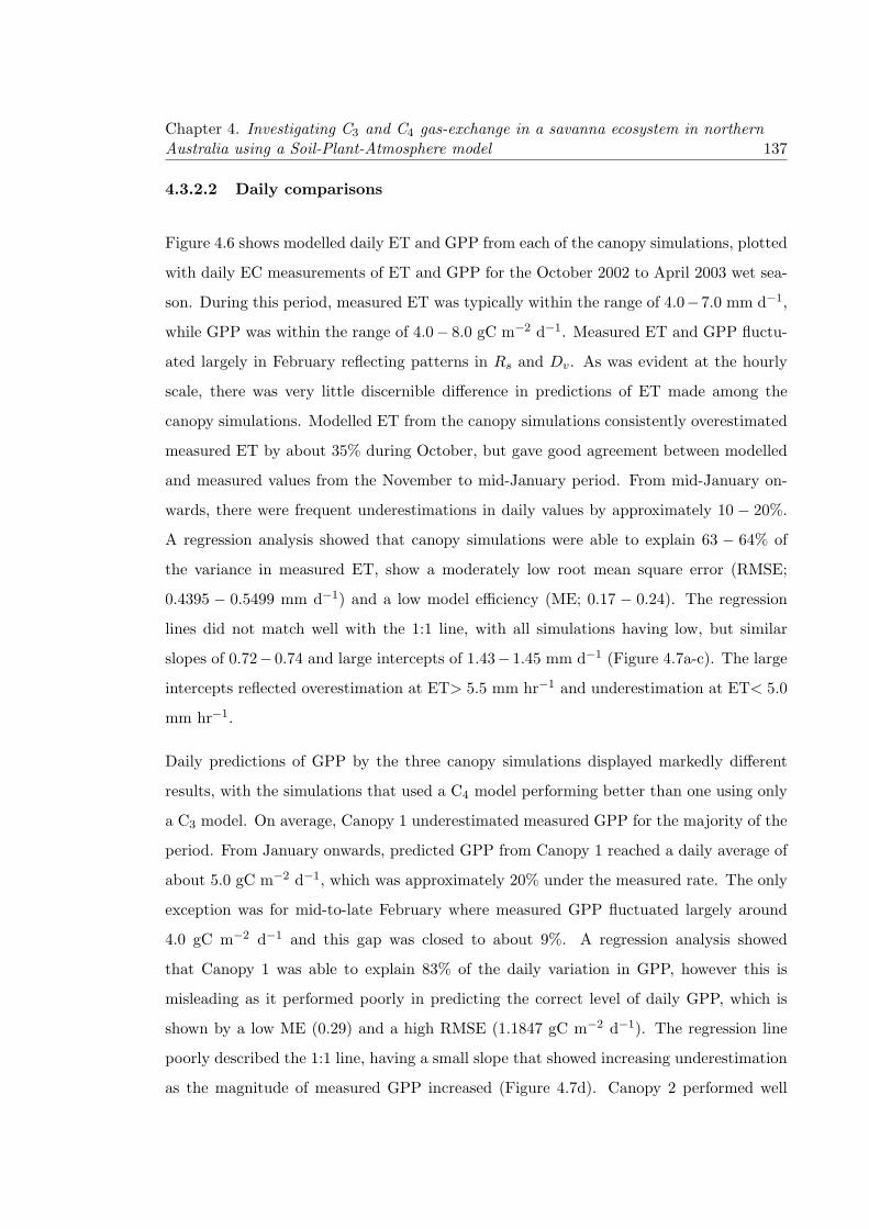
Chapter 4. Investigating C3 and C4 gas-exchange in a savanna ecosystem in northernAustralia using a Soil-Plant-Atmosphere model 137
4.3.2.2 Daily comparisons
Figure 4.6 shows modelled daily ET and GPP from each of the canopy simulations, plotted
with daily EC measurements of ET and GPP for the October 2002 to April 2003 wet sea-
son. During this period, measured ET was typically within the range of 4.0−7.0 mm d−1,
while GPP was within the range of 4.0− 8.0 gC m−2 d−1. Measured ET and GPP fluctu-
ated largely in February reflecting patterns in Rs and Dv. As was evident at the hourly
scale, there was very little discernible difference in predictions of ET made among the
canopy simulations. Modelled ET from the canopy simulations consistently overestimated
measured ET by about 35% during October, but gave good agreement between modelled
and measured values from the November to mid-January period. From mid-January on-
wards, there were frequent underestimations in daily values by approximately 10 − 20%.
A regression analysis showed that canopy simulations were able to explain 63 − 64% of
the variance in measured ET, show a moderately low root mean square error (RMSE;
0.4395 − 0.5499 mm d−1) and a low model efficiency (ME; 0.17 − 0.24). The regression
lines did not match well with the 1:1 line, with all simulations having low, but similar
slopes of 0.72− 0.74 and large intercepts of 1.43− 1.45 mm d−1 (Figure 4.7a-c). The large
intercepts reflected overestimation at ET> 5.5 mm hr−1 and underestimation at ET< 5.0
mm hr−1.
Daily predictions of GPP by the three canopy simulations displayed markedly different
results, with the simulations that used a C4 model performing better than one using only
a C3 model. On average, Canopy 1 underestimated measured GPP for the majority of the
period. From January onwards, predicted GPP from Canopy 1 reached a daily average of
about 5.0 gC m−2 d−1, which was approximately 20% under the measured rate. The only
exception was for mid-to-late February where measured GPP fluctuated largely around
4.0 gC m−2 d−1 and this gap was closed to about 9%. A regression analysis showed
that Canopy 1 was able to explain 83% of the daily variation in GPP, however this is
misleading as it performed poorly in predicting the correct level of daily GPP, which is
shown by a low ME (0.29) and a high RMSE (1.1847 gC m−2 d−1). The regression line
poorly described the 1:1 line, having a small slope that showed increasing underestimation
as the magnitude of measured GPP increased (Figure 4.7d). Canopy 2 performed well

Chapter 4. Investigating C3 and C4 gas-exchange in a savanna ecosystem in northernAustralia using a Soil-Plant-Atmosphere model 138
Figure 4.6: The three model canopies that have been used to simulate daily patterns ofevapotranspiration (ET) and gross primary productivity (GPP) at the Howard Springssavanna site over the October 2002 to November 2003 wet season. The difference betweenthe three different canopy simulations is the photosynthesis model assumed for the grassunderstorey: in Canopy 1 it is C3 and in Canopies 2-3 it is C4. The gray lines and pointsrepresent measured ET and GPP derived from eddy-covariance (EC), while the coloured
lines represent the three different canopy simulations.
in predicting measured GPP, from October to November and January onwards predicting
GPP to be in the range of 5.0 − 7.0 gC m−2 d−1, which was within 9% of the measured
value. Between late November and most of December, the predictions were poor (5.5 gC
m−2 d−1) and underestimated measured GPP by about 15%. Canopy 3 gave almost equal
predictions of GPP compared with Canopy 2; with predictions differing by less than 2%
on average. The only divergence between these two simulations, occurred during the late
November to late December period, where Canopy 3 gave slightly lower predictions at
around 5.0 gC m−2 d−1. A regression analysis showed Canopy 2 to be to explain 84% of
the variation in daily GPP. A high ME (0.70) and low RMSE (0.0393 gC m−2 d−1) gave
a good indication that Canopy 2 performed well in it’s predictions (Figure 4.7e). The
regression was close to the 1:1 line, with a slope of 1.04 and an intercept close to zero.

Chapter 4. Investigating C3 and C4 gas-exchange in a savanna ecosystem in northernAustralia using a Soil-Plant-Atmosphere model 139
Canopy 3 could only explain 69% of the variance which was lower than Canopy 1, but had a
high ME (0.61) and low RMSE (0.0934 gC m−2 d−1), indicating good model performance.
The regression line for Canopy 3 was relatively close to the 1:1 line, with a slightly lower
slope of 0.91 reflecting some slight underestimation of measured GPP (Figure 4.7f).
Figure 4.7: Regression plots that compare modelled and measured evapotranspiration(ET) for (a) Canopy 1, (b) Canopy 2 and (c) Canopy 3 simulations. Additionally, modelledand measured gross primary productivity (GPP) for (d) Canopy 1, (e) Canopy 2 and(c) Canopy 3 are compared. The yellow dotted line represents the 1:1 line, while thesolid blue and red lines represent the fitted regression lines. The difference between thethree different canopy simulations is the photosynthesis model assumed for the grass
understorey: in Canopy 1 it is C3 and in Canopies 2-3 it is C4.
4.3.2.3 Residual analysis
A residual analysis was used to identify the causes of model failure in predicting daily
measured ET and GPP. Plotting the ET residuals against time, showed that underesti-
mation increased moving from the start to the middle of the wet season, before dropping
back to the zero error point at the end of March. This showed the error to be the result

Chapter 4. Investigating C3 and C4 gas-exchange in a savanna ecosystem in northernAustralia using a Soil-Plant-Atmosphere model 140
Table 4.3: Statistics of model performance for the three canopies that were used tosimulate evapotranspiration (ET; *mm d−1) and gross primary productivity (GPP; *gCm−2 d−1) in the Soil-Plant-Atmosphere (SPA) model. The statistics listed here are theexplained variance (R2), model efficiency (ME) and root mean square error (RMSE), slope
and intercept of the regression line.
Model R2 ME RMSE* Slope* Intercept*
ET Canopy 1 0.64 0.24 0.4395 0.72 1.43Canopy 2 0.63 0.17 0.5549 0.73 1.45Canopy 3 0.63 0.18 0.5473 0.74 1.44
GPP Canopy 1 0.83 0.29 1.1847 1.31 0.12Canopy 2 0.84 0.70 0.0393 1.04 0.18Canopy 3 0.69 0.61 0.0934 0.91 -0.54
of one of the environmental drivers during this period (Figure 4.8a). Residuals plotted
against predictions of ET, showed that the error was stable when predictions of ET were
high and underestimation was largely limited when predictions were low (< 3 mm d−1)
(Figure 4.8b). Plotting the ET residuals against the environmental drivers showed that
most of the underestimation is also the result of a drop in total Rs and Dv (Figure 4.8c-d).
The residuals plotted with Dv however, show that at Dv > 3.0 kPa, measured ET is most
likely being reduced by a reduction in canopy gs to prevent xylem cavitation, which is not
being replicated in the model. Residuals plotted against θs and LAI however, show that
increases in canopy LA and soil water stores increased the understimation of ET by the
model (Figure 4.8e-f). In the case of LAI, this could mean that too much LA is being
assigned to the overstorey which is reducing the amount of available energy reaching the
understorey to evaporate water, regardless of θs.
A residual analysis was also used to identify the causes for failure of the photosynthe-
sis models to adequately describe the measured GPP. Differences in intercepts between
Canopy 1 and Canopies 2 and 3, are the result of Canopy 1 consistently underestimating
daily GPP for the period. Plotting the residuals against time showed that underestima-
tion increased from late November to late December period for all simulations (Figure 4.8
g). Plotting the residuals against predicted GPP, showed that the error was not a result
of the magnitude of the predictions in all simulations (Figure 4.8h). Plotted against the

Chapter 4. Investigating C3 and C4 gas-exchange in a savanna ecosystem in northernAustralia using a Soil-Plant-Atmosphere model 141
environmental drivers, the residuals showed a drop in daily total Rs (< 12 MJ m−2 d−1) to
cause an increase in model overestimation of measured GPP for all canopies (Figure 4.8i);
no difference in the slope was seen between the slopes for Canopy 1, 2 and 3 (P < 0.005).
Underestimation of measured GPP increased with increasing Dv (> 3.0 kPa). The un-
derestimation is slightly more pronounced in Canopies 2 and 3, compared with Canopy 1,
which has a slope that is almost zero (Figure 4.8j). Residuals plotted against θs showed
no relationship for Canopies 2 and 3, but a slight relationship to exist for Canopy 1 (Fig-
ure 4.8k). Residuals plotted against LAI showed an irregular curve, where predictions of
GPP decreased between a LAI of 1.4− 1.8 m2 m−2 (Figure 4.8l). Outside this range, the
residuals were well dispersed around the zero error mark, which suggests that the hump is
a product of the other factors (i.e. Dv, Rs). This may therefore not be a problem in the
model, but rather error in the EC measurements (Baldocchi et al., 1996).
4.3.2.4 Comparison of modelled and measured period totals
The cumulative sum of predicted ET and GPP from the three canopy simulations for the
test period were compared against the cumulative sums of the measured period totals
derived from EC (Fig. 4.9). Total measured ET and GPP for the period was 654 mm
and 866 gC m−2 respectively. Canopy 1 overestimated measured total ET by 5.2% at 688
mm, but significantly underestimated total GPP by 19.1% at 701 gC m−2. Canopy 2 gave
the closet approximated totals of measured total ET and GPP. Measured total ET was
overestimated, but only by 3.2% at 675 mm, while total measured GPP was underestimated
by 5.8% at 816 gC m−2. Canopy 3 gave the lowest prediction of total period ET at 591
mm, which was 9.6% under the measured total. However, despite the lower predicted
total ET, Canopy 3 gave a very similar prediction of total GPP at 815 gC m−2, which
was 5.9% under the measured total. This suggests that those simulations which used a C4
photosynthesis model were able to improve their prediction of the estimated total GPP
by 13.3%. This did not have a great affect on estimated totals of ET, which at the worst
was still within 10% of the measured total.

Chapter
4.Investiga
tingC3andC4gas-exch
ange
inasavannaeco
systemin
north
ernAustra
liausin
gaSoil-P
lant-A
tmosphere
model
142
Figure 4.8: Residual analysis between modelled and measured evapotranspiration (ET) and gross primary productivity (GPP) for thethree canopy simulations. The residuals for ET are plotted against (a) time, to determine periods of model failure, (b) model predictions,in order to determine model bias, (c) daily total solar radiation, (d) daily maximum vapour pressure deficit (VPD), (e) daily soil watercontent (SWC) and f) leaf area index (LAI) to determine the influence of the environmental drivers. For the same reasons, residuals ofGPP are plotted against (g) time, (h) model predictions, (i) total solar radiation, (j) VPD, (k) SWC and (l) LAI. For the GPP modelresiduals, Canopy 1 is given by black circles and Canopies 2 and 3 are given by green circles. The red and yellow lines denote a regression
fit to determine a pattern in the residuals.

Chapter 4. Investigating C3 and C4 gas-exchange in a savanna ecosystem in northernAustralia using a Soil-Plant-Atmosphere model 143
Figure 4.9: The cumulative sum of eddy-covariance (EC) measured evapotranspiration(ET) and gross primary productivity (GPP) compared with the cumulative sum of esti-mated ET and GPP derived from the three canopy simulations. These sums are takenover the October 2002 to April 2003 test period. The difference between the three dif-ferent canopy simulations is the photosynthesis model assumed for the grass understorey:
in Canopy 1 it is C3 and in Canopies 2-3 it is C4.
4.3.3 Modelled contributions to savanna fluxes of the C3 overstorey and
C4
The incorporation of the C4 photosynthesis model significantly improved the estimates of
GPP over the simulation period. Canopy 2, using the Collatz et al. (1992) model for C4
photosynthesis having performed the best of the three photosynthesis models in predicting
ecosystem ET and GPP was then applied for the entire five year period (2001–2005) and
compared against EC derived measurements. Additionally, overstorey and understorey
components were examined to examine the relative contribution that the C4 understorey
plays in the savanna ecosystem.
Chapter 4. Investigating C3 and C4 gas-exchange in a savanna ecosystem in northernAustralia using a Soil-Plant-Atmosphere model 144
4.3.3.1 Intra-daily patterns over a one year period
Modelled hourly rates of ET and GPP were compared against EC derived measurements
on a monthly-average diurnal course over the 2001 year. Figure 4.11 was constructed by
binning the hourly diurnal course of modelled and measured ET and GPP by month to
show the average diurnal response for each month across the year. The diurnal course of
measured ET from the wet season to the dry season showed a decrease in midday peak
from 0.30±0.07 mm hr−1 in April to 0.10±0.02 mm hr−1 in September. Peak rates of ET
increased with the arrival of monsoonal rains during late October, reaching a maximum in
December. During the wet season nocturnal water-use was evident, fluctuating between
0.01− 0.02 mm hr−1. Variations in ET were much larger during the wet season (0.20-0.37
mm hr−1) than in the dry (0.11-0.13 mm hr−1) because of frequent cloud cover and high
intermittent rainfall. The diurnal course of measured GPP similarly followed the seasonal
patterns seen in ET. With the onset of the dry season at the start of April, daily peak
GPP fell from a high midday peak of 20.1 ± 4.9 μmol m−2 s−1 to a low midday peak of
5.2 ± 1.3 μmol m−2 s−1 in September, following the seasonal course of LAI (Fig. 4.2b).
The midday peak of GPP increased in late October with the regeneration in canopy LAI
and the onset of frequent rainfall events. By December, canopy vegetation had recovered
from the aridity of the dry season and the GPP midday peak was close to the wet season
average. The model was able to give a good approximation to the diurnal course of
measured ET. During the wet season, ET tended to slightly over- or underestimate across
the year, but generally gave predictions well within the bounds of measurement error.
Predicted seasonal peaks were close to the measured ones, with a similar wet season high
of 0.31 mm hr−1, and dry season low of 0.14 mm hr−1. The only exception occurred during
September and October, where the model significantly overestimated ET above the upper
boundary of error (Figure 4.10a). The model was also able to trace the diurnal course of
measured GPP, matching the monthly-average midday peaks for the majority of the year.
Overestimation tended to be limited to the end of the wet season, when LAI was high and
θs non-limiting, while underestimation tended to occur during the mid-dry season (June–
August), when LAI in the understorey had died off (Figure 4.10b). However, in most cases
these variations were within the bounds of error. The model was able to predict similar

Chapter 4. Investigating C3 and C4 gas-exchange in a savanna ecosystem in northernAustralia using a Soil-Plant-Atmosphere model 145
high midday peaks of GPP (22.5 μmol m−2 s−1) during the wet season, and match the
low midday-peak of 5.2 μmol m−2 s−1 well into the dry season.
In order to examine how canopy gas-exchange in the savanna differs between the C3 and C4
parts of the canopy, the canopy predictions in Figure 4.10 were partitioned into tree (C3)
and grass (C4) transpiration (Et) and An. Additionally the leaf-scale variables of gs and
Ψl were used to help explain the seasonal variations (Figure 4.11). Wet and dry season
patterns of overstorey stomatal conductance (C3gs) were asymmetrical over the diurnal
course, with a much higher C3gs in the morning than in the afternoon (Figure 4.11a).
Maximum wet season C3gs peaked at approximately 0.6 mol m−2 s−1 in the morning and
decreased to around 0.4 mol m−2 s−1 in the afternoon, due to tight stomatal control in
response to the drop in Ψl. Morning peak C3gs during the dry season did not reach the
high levels achieved in the wet season and were limited to around 0.40 mol m−2 s−1, being
regulated by low overstorey Ψl. The distinct asymmetry in the diurnal course of C3gs
observed in the wet season was not as severe in the dry season, and afternoon C3gs did not
reduce by a significant amount falling to about 0.3 mol m−2 s−1. Understorey stomatal
conductance (C4gs), maintained a relatively constant maximum at around 0.25 mol m−2
s−1, with the exception of April which displayed a higher than average peak at about 0.4
mol m−2 s−1. No asymmetry was observed in the diurnal courses of monthly C4gs, due to
high Ψl and low Dv. As the canopy moved into the dry season C4gs dropped from a high
in April to a low in May following the severe drop in leaf area.
Patterns in the diurnal course of Et in both the C3 tree canopy and C4 grasses reflected
changes in gs and Ψl (Figure 4.11b). The overstorey transpiration rate (C3Et) remained
fairly consistent over the course of the year at about 1.1 mmol m−2 s−1, but increased
during the wet-to-dry season transition period (April–June) to a high of 1.6 mmol m−2
s−1 as a result of high θs, large Rs and an increased Dv. However as Ψl dropped, so too
did C3Et due to tighter stomatal control reaching a low of about 0.8 mmol m−2 s−1 in
the dry season. The understorey transpiration rate (C4Et) was relatively low and constant
during the wet season, maintaining an hourly maximum C4Et of 0.4 mmol m−2 s−1. There
was an increase in C4Et to approximately 0.5 mmol m−2 s−1 moving out of the dry season
(due to increasing LAI with θs), but this declined to a constant of 0.4 mmol m−2 s−1 with
the seasonal drop in Dv.

Chapter
4.Investiga
tingC3andC4gas-exch
ange
inasavannaeco
systemin
north
ernAustra
liausin
gaSoil-P
lant-A
tmosphere
model
146
Figure 4.10: Binned monthly diurnal patterns of modelled (a) evapotranspiration (ET) and (b) gross primary productivity (GPP)compared with measurements derived from eddy-covariance (EC) for 2001. The mean measured responses of ET and GPP are given asblack lines, while model predictions are given as red lines. The shaded gray regions denote the standard deviation of the measured mean
ET and GPP.

Chapter
4.Investiga
tingC3andC4gas-exch
ange
inasavannaeco
systemin
north
ernAustra
liausin
gaSoil-P
lant-A
tmosphere
model
147
Figure 4.11: Binned monthly diurnal patterns of the simulated C3 tree canopy and C4 grass averaged leaf-scale gas-exchange quantitiesin 2001. These quantities include (a) the weighted stomatal conductance (gs), (b) transpiration (Et), (c) net assimilation (An) and (d) leaf
water potential (Ψl). The red lines denote the C3 tree canopy, while the blue lines represent the C4 grasses.

Chapter 4. Investigating C3 and C4 gas-exchange in a savanna ecosystem in northernAustralia using a Soil-Plant-Atmosphere model 148
Net CO2 assimilation rates in the over- and understorey strongly reflected seasonal changes
in over- and understorey LAI (Figure 4.2b). Overstorey net assimilation (C3An) remained
consistent over the wet season period, with a midday peak of 10.1 μmol m−2 s−1, with the
exception of the dry-to-wet season transitional period (October–December) where C3An
was lower (Figure 4.11c). Dry season C3An reached a reduced maximum of 4.0 μmol m−2
s−1 during September and is likely a result of a very low Ψl tracking close to the Ψl min
restricting stomatal opening. Understorey net assimilation (C4An) was high during the
wet season, where peak rates were 10.3 μmol m−2 s−1, equivalent with the overstorey.
Following the seasonal course of LAI, C4An dropped significantly in May to a peak rate
< 1 μmol m−2 s−1. Rates of C4An increased gradually during the dry-to-wet transition
period to reach large wet season rates in January.
Leaf water potentials between the canopy over- and understorey were significantly different
over the course of the year (Figure 4.11d). Overstorey minimum leaf water potential (C3Ψl)
was highest during the wet season with the highest C3Ψl occuring in February at about
-1.75 MPa. Moving into the dry season C3Ψl decreased to an average low of -2.4 MPa
tracking close to Ψl min due to consistent water-use by the overstorey through the dry
season at low soil moisture. In actuallity C3Ψl would have fallen below Ψl min frequently,
causing a stronger stomatal regulation to water loss. Conversely, understorey leaf water
potential (C4Ψl) remained relatively high during the wet season, staying above -1.0 MPa
for most months, with the exception of the dry-to-wet transition period which reached an
average minimum of -2.0 MP as a result of low soil moisture in the upper soil profile. C4Ψl
decreased with the increase in soil moisture of the upper soil profile, due the increased
frequency of rainfall events. High C4Ψl was maintained due to low C4Et as a result of the
C4 photosynthetic pathway being highly water-use efficient.
Abiotic factors controlling canopy gas-exchange
The tree overstorey (C3) and grass understorey (C4) outputs of Et and An described
above were plotted against four key abiotic variables known to regulate these fluxes, as a
way of investigating how they responsed to changes in the environment. In the wet-dry
tropics of Australia, variables known to drive water loss and carbon assimilation are Rs,

Chapter 4. Investigating C3 and C4 gas-exchange in a savanna ecosystem in northernAustralia using a Soil-Plant-Atmosphere model 149
Dv and θs (Eamus et al., 2001). Figure 4.12 shows the response of tree over- and grass
understorey rates of Et and An to variation in these variables, as well as LAI. Quantile
regression (Koenker and Bassett, 1978) was used to fit a set of nonlinear relationships for
the responses of modelled over- and understorey An and Et to variation in Rs and Dv,
and linear relationships were used to explain the variation in θs and LAI. Fitting the 95%
quantile of these relationships rather than the mean was done in order to capture the non-
limiting responses of over and understorey gas-exchange to the driving abiotic variables
(e.g. the response of An to Rs independent of Dv, θ and LAI) (Jarvis, 1976; Stewart, 1988;
Makela et al., 2008).
Modelled C3 over- and C4 understorey An increased linearly with Rs until approximately
200 W m−2 where it tended towards an asymptote, saturating towards Amax at Rs > 800
W m−2 (Figure 4.12a). The understorey exhibited a slightly larger initial slope (pro-
portional to ecosystem quantum yield) compared with the overstorey. Despite a drop in
Amax, no discernible difference was observed in the slope between the wet and dry season
responses (Figure 4.12b). In contrast, a significant difference was observed between the
over- and understorey responses of Et to variation in Rs. The response of overstorey Et
in the wet season showed an asymptotic response similar to that of An, but saturated
towards Emax (1.6 mmol m−2 s−1) at a much larger Rs (≈ 900 W m−2). The under-
storey response on the other hand was linear, with no observable asymptote observed
(Figure 4.12c). The dry season response for the overstorey exhibited a linear increase at
low Rs and Emax approached an asymptote much sooner than in the wet season (≈ 300
W m−2) (Figure 4.12d).
The modelled C3 over- and C4 understorey responses of An to Dv in the wet season showed
rapid increases in An at low Dv, reaching Amax at approximately 1.0 kPa, after which a
rapid decline was observed when Dv > 1.5 (Figure 4.12e). No difference in the slopes
between the overstorey and understorey was observable, with both canopy components
tending to exhibit the same rate of decay in An. There was a very weak overstorey response
in the dry season, with no significant relationship being determined, except for a slight
drop in An when Dv > 2.5 kPa (Figure 4.12f). The response of over- and understorey Et
to increasing Dv during the wet season was more pronounced than that of An. Overstorey
Et increased linearly at low values of Dv, reaching Emax at approximately 1.5 kPa, after

Chapter 4. Investigating C3 and C4 gas-exchange in a savanna ecosystem in northernAustralia using a Soil-Plant-Atmosphere model 150
which it declined linearly (Figure 4.12g). However, understorey Et reached Emax at a
much higher Dv and did not decline with increasing Dv in contrast to the overstorey. Dry
season overstorey Et increased linearly to a much higher Dv than in the wet season at
approximately 3.0 kPa, but experienced a sharp decline after this value (Figure 4.12h).
Figure 4.12: Relationships between modelled wet and dry season estimates of C3 andC4 net assimilation (An) and transpiration (Et) and the primary environmental driversof solar radiation (a-d) (Rs), (e-h) vapour pressure deficit (Dv), (i-l) soil water content(θs) and (m-p) leaf area index (LAI). The black circles shows model estimates for theC3 trees, and the white circles show the model estimates for the C4 grasses. Quantileregression is used to fit the upper boundaries of the relationships in order to determinethe underyling non-limiting responses, where the red and blue lines represent the quantile
fits for C3 and C4 vegetation respectively.
The over- and understorey responses of An to increasing θs displayed piece-wise linear
relationships, with the slope of the relationship being slightly larger in the understorey

Chapter 4. Investigating C3 and C4 gas-exchange in a savanna ecosystem in northernAustralia using a Soil-Plant-Atmosphere model 151
than in the overstorey (Figure 4.12i). In contrast, the overstorey response in the dry season
displayed no significant relationship, despite a much lower θs, likely due to the overstorey
accessing deep water-stores (Figure 4.12j). The wet season response of overstorey Et
displayed a similar broken stick relationship and similar slope to that of An (Figure 4.12k).
No significant relationship for understorey Et was observed in the wet season, suggesting
that the C4 grasses are insensitive to soil water status. In the dry season no significant
response was observed for the overstorey (Fig. 4.12l). It should be noted that the soil
moisture measurements are only for the top 10 cm of the soil profile and no true response
may be seen for both An and Et in either season. It is therefore recommended that Figures
4.12i-l) be interpreted with caution.
Relationships between modelled over- and understorey An and LAI showed strong positive
linear responses (Figure 4.12m). Both over- and understorey sections of the canopy dis-
played similar slopes in the relationship, with the understorey being slightly higher. The
dry season response of the overstorey showed a strong relationship with LAI, producing a
larger slope than in the wet season (Figure 4.12n). The wet season responses of over- and
understorey Et were markedly different, with the overstorey showing a strong significant
relationship, and the canopy understorey showing no relationship (Figure 4.12o). For the
dry season a significant response of the overstorey was observed (Figure 4.12p). Strong
relationships for overstorey An and Et in the dry season, is most likely due to adjustment
of the canopy leaf-area in response to seasonal changes in Dv and θ. All modelled gas-
exchange responses were found to have the same Amax and Emax across the 4 covariates.
4.3.3.2 Seasonal patterns over the 2001 to 2005 period
Total Canopy
Daily outputs of predicted ET and GPP from SPA were compared against EC derived
measurements for the 2001 to 2005 study period (Figure 4.13). Ecosystem ET and GPP
derived from EC measurements were largest in the wet season, typically within the ranges
of 3.5-7.0 mm d−1 and 4.0-8.0 gC m−2 d−1 respectively; only rarely did GPP decline below
3.0 gC m−2 d−1 in the wet season. Day-to-day variations in ET and GPP in the wet season

Chapter 4. Investigating C3 and C4 gas-exchange in a savanna ecosystem in northernAustralia using a Soil-Plant-Atmosphere model 152
closely reflected patterns in rainfall and Rs. From approximately mid-March through to
September, both ET and GPP declined exponentially to an approximate minimum of 2.0
mm d−1 and 1.5 gC m−2 d−1 respectively. In the singular case of 2001, ET declined to an
approximate low of 0.5 mm d−1. Gradual increases in ET and GPP began following the
dry season minima, generally between late September and mid-October, following the new
growth of C4 vegetation. The model predicted maximum ET in the wet season at values
between 4.0 and 7.0 mm d−1, while minimum values slightly overestimated dry season
ET; predicting values within the range of 2.0-3.0 mm d−1. It was only in 2003 that the
model was able to clearly match measured dry season ET, with overestimation occurring
for all other dry seasons. Model predictions of daily GPP match well with the EC derived
measurements for the five year simulation period. The model predicted a maximum GPP
of approximately 7.5 gC m−2 d−1 in the wet season agreeing well with the measurements.
During the dry season predicted GPP fell to a minimum of 1.5 gC m−2 d−1 in September.
The model was able to predict variations shown in the measurements especially in 2001
and 2003. The other years however had higher measured minimums of about 2.0-2.5 gC
m−2 d−1, which the model underestimated.
A regression analysis between modelled fluxes of ET and GPP and the EC derived mea-
surements was done for each separate year and the entire simulation period (Figure 4.14).
Plots of modelled versus measured are given for each year used in the simulation.3 Fig-
ure 4.14 shows that across all five years of study, there was a significant positive relationship
between modelled and measured for both GPP and ET; these statistics are given in Ta-
ble 4.4. Modelled ET produced a moderate range of R2 values, and was able to explain
68-81% of the variation in measured ET across the study period and explained 75% of
the variance over the entire five years. The ME showed that out of these years, 2001 and
2002 gave close approximations to the 1:1 line with ME values in the range of 58 to 65.
This was reflected in low values of RMSE in the range of 0.0656− 0.1205 mm d−1, slopes
closest to 1 and intercepts closest to 0. The years of 2003-2005 had much lower ME values
in the range of 0.44 to 0.49. However, the RMSE was still low for these years, in the range
of 0.0500-0.1929 mm d−1, and the regression lines had reduced slopes and slightly larger
intercepts. For the entire period, the model was able to explain 75% of the variance, but
3ET is plotted along a positive scale, while GPP is plotted against a negative scale

Chapter
4.Investiga
tingC3andC4gas-exch
ange
inasavannaeco
systemin
north
ernAustra
liausin
gaSoil-P
lant-A
tmosphere
model
153
Figure 4.13: A comparison of estimated (red line) evapotranspiration (EC) and gross primary productivity (GPP) using the Soil-Plant-Atmosphere (SPA) model with the measured (black line) ET and GPP derived from eddy-covariance (EC) for the 2001 to 2005 study
period. The yellow shaded regions denote the dry season period for each year.
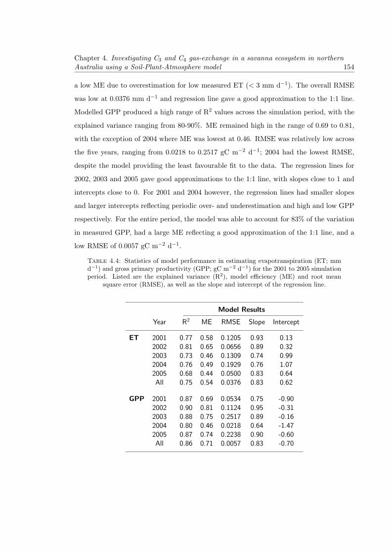
Chapter 4. Investigating C3 and C4 gas-exchange in a savanna ecosystem in northernAustralia using a Soil-Plant-Atmosphere model 154
a low ME due to overestimation for low measured ET (< 3 mm d−1). The overall RMSE
was low at 0.0376 mm d−1 and regression line gave a good approximation to the 1:1 line.
Modelled GPP produced a high range of R2 values across the simulation period, with the
explained variance ranging from 80-90%. ME remained high in the range of 0.69 to 0.81,
with the exception of 2004 where ME was lowest at 0.46. RMSE was relatively low across
the five years, ranging from 0.0218 to 0.2517 gC m−2 d−1; 2004 had the lowest RMSE,
despite the model providing the least favourable fit to the data. The regression lines for
2002, 2003 and 2005 gave good approximations to the 1:1 line, with slopes close to 1 and
intercepts close to 0. For 2001 and 2004 however, the regression lines had smaller slopes
and larger intercepts reflecting periodic over- and underestimation and high and low GPP
respectively. For the entire period, the model was able to account for 83% of the variation
in measured GPP, had a large ME reflecting a good approximation of the 1:1 line, and a
low RMSE of 0.0057 gC m−2 d−1.
Table 4.4: Statistics of model performance in estimating evapotranspiration (ET; mmd−1) and gross primary productivity (GPP; gC m−2 d−1) for the 2001 to 2005 simulationperiod. Listed are the explained variance (R2), model efficiency (ME) and root mean
square error (RMSE), as well as the slope and intercept of the regression line.
Model Results
Year R2 ME RMSE Slope Intercept
ET 2001 0.77 0.58 0.1205 0.93 0.132002 0.81 0.65 0.0656 0.89 0.322003 0.73 0.46 0.1309 0.74 0.992004 0.76 0.49 0.1929 0.76 1.072005 0.68 0.44 0.0500 0.83 0.64All 0.75 0.54 0.0376 0.83 0.62
GPP 2001 0.87 0.69 0.0534 0.75 -0.902002 0.90 0.81 0.1124 0.95 -0.312003 0.88 0.75 0.2517 0.89 -0.162004 0.80 0.46 0.0218 0.64 -1.472005 0.87 0.74 0.2238 0.90 -0.60All 0.86 0.71 0.0057 0.83 -0.70
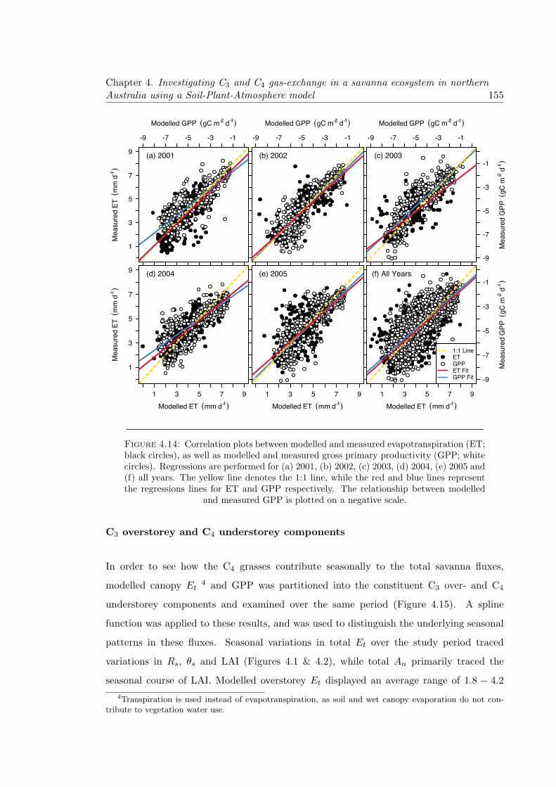
Chapter 4. Investigating C3 and C4 gas-exchange in a savanna ecosystem in northernAustralia using a Soil-Plant-Atmosphere model 155
Figure 4.14: Correlation plots between modelled and measured evapotranspiration (ET;black circles), as well as modelled and measured gross primary productivity (GPP; whitecircles). Regressions are performed for (a) 2001, (b) 2002, (c) 2003, (d) 2004, (e) 2005 and(f) all years. The yellow line denotes the 1:1 line, while the red and blue lines representthe regressions lines for ET and GPP respectively. The relationship between modelled
and measured GPP is plotted on a negative scale.
C3 overstorey and C4 understorey components
In order to see how the C4 grasses contribute seasonally to the total savanna fluxes,
modelled canopy Et4 and GPP was partitioned into the constituent C3 over- and C4
understorey components and examined over the same period (Figure 4.15). A spline
function was applied to these results, and was used to distinguish the underlying seasonal
patterns in these fluxes. Seasonal variations in total Et over the study period traced
variations in Rs, θs and LAI (Figures 4.1 & 4.2), while total An primarily traced the
seasonal course of LAI. Modelled overstorey Et displayed an average range of 1.8 − 4.2
4Transpiration is used instead of evapotranspiration, as soil and wet canopy evaporation do not con-tribute to vegetation water use.
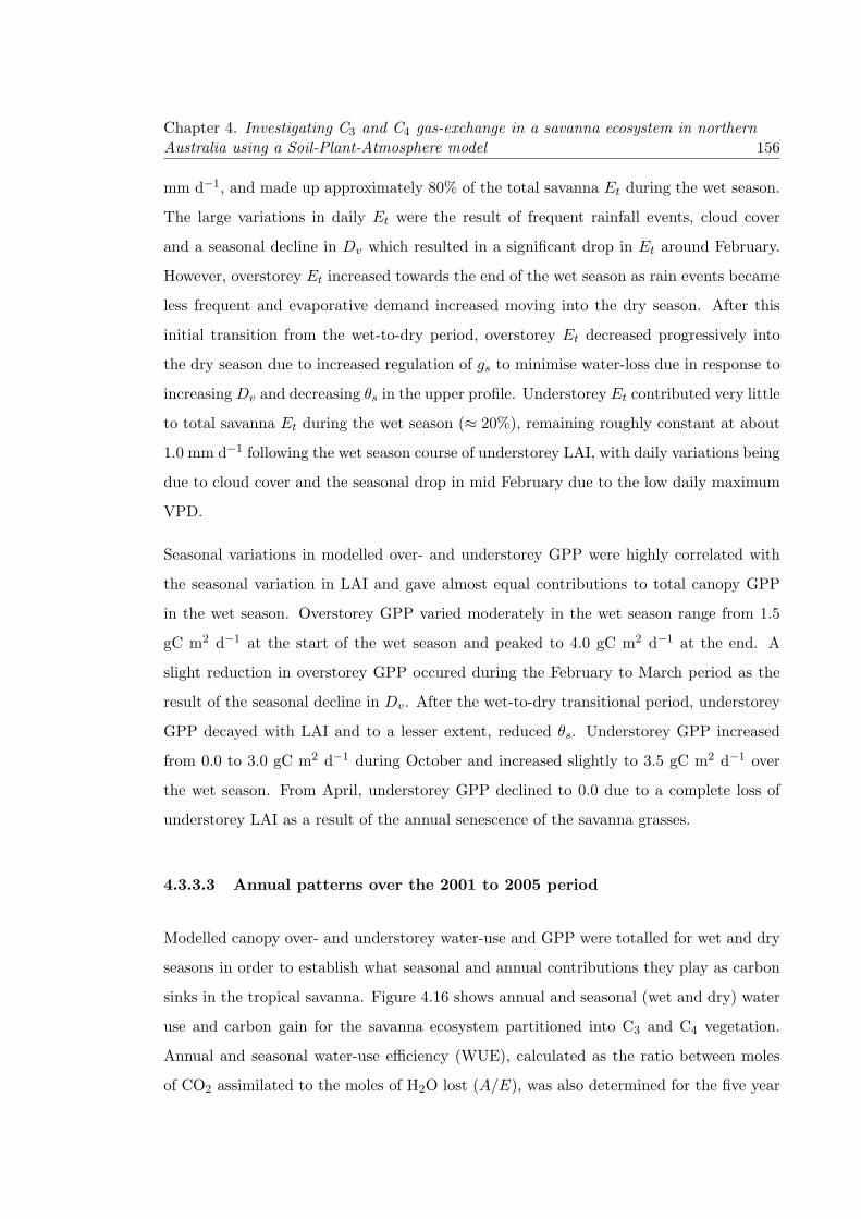
Chapter 4. Investigating C3 and C4 gas-exchange in a savanna ecosystem in northernAustralia using a Soil-Plant-Atmosphere model 156
mm d−1, and made up approximately 80% of the total savanna Et during the wet season.
The large variations in daily Et were the result of frequent rainfall events, cloud cover
and a seasonal decline in Dv which resulted in a significant drop in Et around February.
However, overstorey Et increased towards the end of the wet season as rain events became
less frequent and evaporative demand increased moving into the dry season. After this
initial transition from the wet-to-dry period, overstorey Et decreased progressively into
the dry season due to increased regulation of gs to minimise water-loss due in response to
increasingDv and decreasing θs in the upper profile. Understorey Et contributed very little
to total savanna Et during the wet season (≈ 20%), remaining roughly constant at about
1.0 mm d−1 following the wet season course of understorey LAI, with daily variations being
due to cloud cover and the seasonal drop in mid February due to the low daily maximum
VPD.
Seasonal variations in modelled over- and understorey GPP were highly correlated with
the seasonal variation in LAI and gave almost equal contributions to total canopy GPP
in the wet season. Overstorey GPP varied moderately in the wet season range from 1.5
gC m2 d−1 at the start of the wet season and peaked to 4.0 gC m2 d−1 at the end. A
slight reduction in overstorey GPP occured during the February to March period as the
result of the seasonal decline in Dv. After the wet-to-dry transitional period, understorey
GPP decayed with LAI and to a lesser extent, reduced θs. Understorey GPP increased
from 0.0 to 3.0 gC m2 d−1 during October and increased slightly to 3.5 gC m2 d−1 over
the wet season. From April, understorey GPP declined to 0.0 due to a complete loss of
understorey LAI as a result of the annual senescence of the savanna grasses.
4.3.3.3 Annual patterns over the 2001 to 2005 period
Modelled canopy over- and understorey water-use and GPP were totalled for wet and dry
seasons in order to establish what seasonal and annual contributions they play as carbon
sinks in the tropical savanna. Figure 4.16 shows annual and seasonal (wet and dry) water
use and carbon gain for the savanna ecosystem partitioned into C3 and C4 vegetation.
Annual and seasonal water-use efficiency (WUE), calculated as the ratio between moles
of CO2 assimilated to the moles of H2O lost (A/E), was also determined for the five year
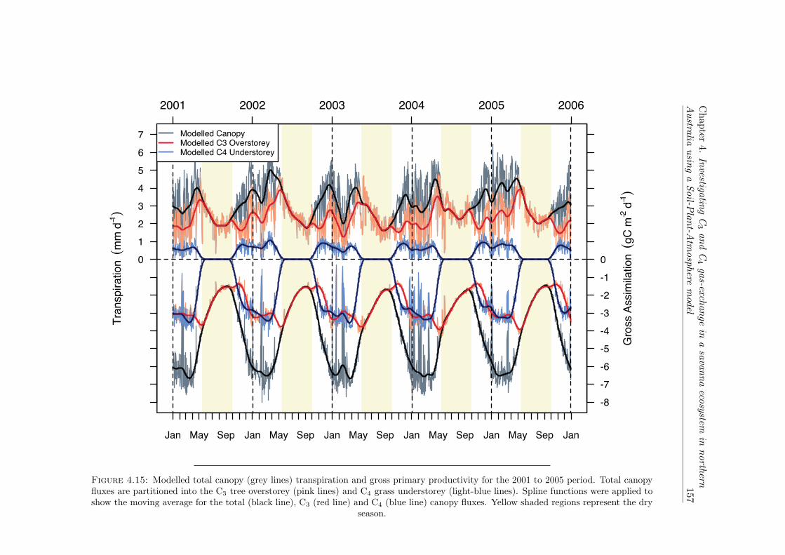
Chapter
4.Investiga
tingC3andC4gas-exch
ange
inasavannaeco
systemin
north
ernAustra
liausin
gaSoil-P
lant-A
tmosphere
model
157
Figure 4.15: Modelled total canopy (grey lines) transpiration and gross primary productivity for the 2001 to 2005 period. Total canopyfluxes are partitioned into the C3 tree overstorey (pink lines) and C4 grass understorey (light-blue lines). Spline functions were applied toshow the moving average for the total (black line), C3 (red line) and C4 (blue line) canopy fluxes. Yellow shaded regions represent the dry
season.

Chapter 4. Investigating C3 and C4 gas-exchange in a savanna ecosystem in northernAustralia using a Soil-Plant-Atmosphere model 158
period. Finally, annual and seasonal light-use efficiency (LUE), calculated as the ratio
between moles of CO2 assimilated to the moles of absorbed photons (A/APAR), was
determined in order to determine the efficiency of the utilisation of light by the canopy
and its over- and understorey components. Values for these measurements are given in
Table 4.5.
Annual measured totals of ET were within a range of 1052-1213 mm (2001, 2004) over
the five year period. This was made up of wet and dry season totals which were in the
ranges of 826-901 mm (2003, 2002) and 207-324 mm (2001, 2004) respectively. Modelled
totals of ET were overestimated across all years and seasons, with an annual range of
1181-1352 mm of water (2003, 2002) over the five year period. Modelled seasonal totals
also overestimated measured totals, predicting a range of 850-1021 mm (2003, 2002) for
the wet season and 331-378 mm (2002, 2004) for the dry season. Annual measured totals
of total GPP were within a range of 1409-1560gC m−2 (2003, 2005), which was made up
of wet and dry season totals in the range of 1082-1232 gC m−2 (03,05) and 289-385 gC
m−2 (2002, 2004) respectively. Modelled totals of annual and seasonal GPP were within
10% of the measured totals over the five year period. Modelled carbon uptake by the
ecosystem and canopy were deemed equivalent, as carbon uptake or release by the soil is
not accounted for in the model. The model predicted the vegetation to sequester 1440-
1501 gC m−2 (2001, 2003) annually, 1186-1214 gC m−2 (2001, 2005) during the wet season
and 254-299 gC m−2 (2001, 2003) during the dry season. The canopy transpired 803-914
mm of water (2003, 2002) annually, 571-670 mm (2001, 2002) during the wet season, and
243-285 mm (2001, 2004) in the dry season in order to achieve these levels of carbon gain.
The C3 canopy overstorey sequestered 869-943 gC m−2 (2001, 2004) annually, 635-650 gC
m−2 (2001, 2004) during the wet season, and 254-299 gC m−2 (2001, 2003) during the dry
season. On average the overstorey canopy accounted for 53% of total wet season GPP and
62% of total annual GPP. The amount of water lost from the canopy overstorey to maintain
this level of carbon uptake was in the range of 683-762 mm (2001, 2002) annually, 425-
510 mm (2003, 2002) in the wet season, and 243-285 mm (2001, 2004) in the dry season.
This averaged to the overstorey canopy accounting for 77% of the water lost during the
wet season, and 35 − 38% of the total water lost in evapotranspiration annually. Totals
of GPP for the C4 grass understorey were slightly less than the overstorey, sequestering

Chapter
4.Investiga
tingC3andC4gas-exch
ange
inasavannaeco
systemin
north
ernAustra
liausin
gaSoil-P
lant-A
tmosphere
model
159Figure 4.16: Modelled and measured period totals of savanna water-use (ET) and gross primary productivity (GPP) for the 2001 to 2005study period. Modelled savanna fluxes are estimated from the Soil-Plant-Atmosphere (SPA) model, while measured fluxes are derived fromeddy-covariance (EC). Totals derived from EC and SPA are given at the (a) annual (T), wet (W) and dry (D) season time-steps. Estimated(b) wet and (c) dry season totals of transpiration and GPP are partitioned from total canopy (C) into C3 (O) and C4 (U) components.

Chapter
4.Investiga
tingC3andC4gas-exch
ange
inasavannaeco
systemin
north
ernAustra
liausin
gaSoil-P
lant-A
tmosphere
model
160
Table 4.5: Table of modelled annual, wet and dry season totals of water-use and carbon uptake for the 2001 to 2005 period. Additionally,canopy water-use (WUE) and light-use efficiency (LUE) are given. Totals are partitioned from the total ecosystem (Eco), to total vegetation
(Can), and into C3 overstorey (Ovr) and C4 understorey (Und).
Annual Wet Season Dry Season
Year Eco Can Ovr Und Eco Can Ovr Und Eco Can Ovr Und
Water Use (mm) 2001 1243 805 674 131 926 571 440 131 317 234 234 02002 1352 914 754 160 1021 670 510 160 331 244 244 02003 1181 803 673 130 850 555 425 130 331 248 248 02004 1320 867 727 140 941 591 451 140 378 276 276 02005 1307 881 733 148 968 634 486 148 339 247 247 0
Carbon Uptake (gC m−2) 2001 1440 1440 869 567 1186 1186 635 567 254 254 254 02002 1465 1465 902 571 1204 1204 641 571 261 261 261 02003 1501 1501 942 573 1202 1202 643 573 299 299 299 02004 1498 1498 943 564 1202 1202 650 564 293 293 293 02005 1475 1475 909 575 1214 1214 648 575 261 261 261 0
WUE (mmol CO2 mol−1 H2O ) 2001 2.68 1.93 6.49 3.12 2.16 6.49 1.63 1.63 02002 2.40 1.79 5.35 2.70 1.89 5.35 1.60 1.60 02003 2.80 2.10 6.61 3.25 2.97 6.61 1.81 1.81 02004 2.59 1.95 6.04 3.05 2.16 6.04 1.59 1.59 02005 2.51 1.86 5.83 2.87 2.00 5.83 1.59 1.59 0
LUE (mol CO2 mol−1 photon ) 2001 0.0201 0.0164 0.0305 0.0221 0.0181 0.0305 0.0142 0.0142 02002 0.0205 0.0170 0.0307 0.0224 0.0182 0.0307 0.0146 0.0146 02003 0.0210 0.0178 0.0308 0.0224 0.0183 0.0308 0.0168 0.0168 02004 0.0209 0.0178 0.0303 0.0224 0.0185 0.0303 0.0164 0.0164 02005 0.0206 0.0172 0.0309 0.0226 0.0184 0.0309 0.0146 0.0146 0

Chapter 4. Investigating C3 and C4 gas-exchange in a savanna ecosystem in northernAustralia using a Soil-Plant-Atmosphere model 161
from 564-573 gC m−2 (2004, 2003) in the wet season, which on average accounted for
47% of the total wet season GPP and 38% of the total annual GPP. The understorey was
highly water-use efficient, transpiring only 130-160 mm of water (2003, 2002) during the
wet season despite the large carbon gains, only accounting for 23% of the total water lost
from the ecosystem and during the wet season and made up only 11− 12% of total annual
evapotranspiration.
The annual WUE of the canopy varied only slightly within the range of 2.40-2.80 mmols
CO2 mols−1 H2O (2002, 2003). Removing the grass understorey component, leaving just
the tree overstorey, reduced WUE to a much lower range of 1.51-1.82 mmols CO2 mols−1
H2O (2002, 2003). Solely considering the wet season periods, the total canopy WUE
increased to 2.70-3.25 mmols CO2 mols−1 H2O (2002, 2003), while partitioning the canopy
into over- and understorey parts shows the understorey to be highly efficient, having a
WUE almost triple that of the overstorey, in the range of 5.35-6.61 mmols CO2 mols−1
H2O (2002, 2003). During the dry season WUE droped by approximately half for the
overstorey canopy, producing a range of 1.59-1.81 mmols CO2 mols−1 H2O (2004, 2003),
which was in response to an inactive understorey (grasses dead), reduced soil water supply
and hence trees became more conservative in their water use.
Differences in canopy LUE were evident between wet and dry season period across all years,
with a range of 0.2206-0.2258 mols CO2 mols−1 photon (2001, 2005) in the wet season,
which was 50% larger than observed in the dry season at 0.1424-0.1676 mols CO2 mols−1
photon (2001, 2003). Comparing over- and understorey LUE in the wet season, shows
the understorey to be more efficient in utilising available light; 0.3030-0.3078 mols CO2
mols−1 photon (Understorey; 2004, 2003) compared to 0.1824-0.1850 mols CO2 mols−1
photon (Overstorey; 2002, 2004). The higher LUE in the understorey is a product of the
higher carbon yields and lower absorbed light by the grasses. Differences in LUE among
years was statistically insignificant (ANOVA; P > 0.05) despite variability in wet and dry
season lengths.
Chapter 4. Investigating C3 and C4 gas-exchange in a savanna ecosystem in northernAustralia using a Soil-Plant-Atmosphere model 162
4.4 Discussion
The purpose of this study was to successfully incorporate a provision for C4 vegetation
within the SPA model, thereby allowing its application to savannas, as well as to provide
a way of investigating the contribution of C4 photosynthesis in the savanna ecosystem.
Adding a C4 photosynthetic sub-model gave a significant improvement in seasonal esti-
mates of GPP via a larger An from the C4 photosynthetic pathway. Additionally, this did
not impact seasonal estimates of ET. The ability to describe variations in the seasonal
distribution of LAI through an input matrix was also an important improvement, as the
senescent nature of the C4 grasses could be approximated for and handled by the model
during the simulation period. Lastly, using SPA to fit a BBL-type relationship was an
effective method in determining C3ιop and C4ιop at this site; a necessary parameterisation
that constrained C4gs to values that are characteristic of plants using this photosynthetic
pathway.
4.4.1 Modelled C3 and C4 stomatal efficiency
An important component of this study was in carefully and correctly parameterising the
C4 understorey that was present at this site. By simulating gs and An over a range of
Qp at different levels of ιop, outputs could be compared with leaf-scale measurements
using a BBL relationship, where the correct level for ιop matches a1 slope parameter of
the measured data. This allowed the determination of both C3ιop and C4ιop at this site.
Although this value is a freely adjustable input in the model, the methodology given here
does give a means of quantifying ιop for particular vegetation types or the study site in
particular. However, some unexpected inconsistencies did occur when applying the method
to C4 vegetation. The relationships were curved rather than linear (compared with the C3
relationships) and this curvature increased with increasing ιop. This may be related to the
characteristic of C4 photosynthesis to not saturate until high light levels (Collatz et al.,
1992) or gs being insensitive to Dv at low values (Leuning, 1995; Monteith, 1995). Either
or both possible causes were not clearly apparent in the measured data, but when tested
with the von Caemmerer and Furbank (1999) C4 model as well, the same curvature was
still present, so it is most likely due in part to a characteristic of the C4 pathway.

Chapter 4. Investigating C3 and C4 gas-exchange in a savanna ecosystem in northernAustralia using a Soil-Plant-Atmosphere model 163
The ιop parameter has been parametrised in previous studies. Williams et al. (1996a)
selected their ιop in accordance with a desired maximum rate of gs observed with measure-
ments of northern red oak (Quercus rubra), which they believed to be 0.07%. Additionally,
they used a sensitivity analysis in testing ιop at relative levels from this value, with their
value of 0.07% giving the best balance between water loss and carbon gain. They also
found ιop to be highly influential on the predictions of ET. However, in the present study
this was not apparent. This may be in part due to this site having abundant soil water
stores; in this study ιop was parameterised for the wet season when the C4 grasses were
active. Similarly, Misson et al. (2004) parametrised ιop for a very simplified version of
the SPA stomatal model, by fitting it to measured gs and found a slightly higher value
of ιop = 0.10% to be most appropriate in matching measurements taken for ponderosa
pine (Pinus ponderosa Dougl. ex Laws.). Although these methods of determining ιop are
feasible, the method described in this chapter is able to quantify the value of ιop with the
well established BBL relationship. It appears that for three very different tree species,
C3ιop had a range of 0.07− 0.10%, and this may be reasonable range for most C3 species
in balancing water-loss and carbon gain without significant penalty.
This study is the first that attempts to parameterise ιop for C4 plants and the value
derived here can not be compared with other studies. However, a comparison can be
drawn with the C3 ιop values. The higher ιop derived for C4 plants is very likely, as they
are by nature, very water conservative and a default ιop = 0.07% is most likely too high
for this photosynthetic pathway. Based on the above comparison of the parametrised
ιop for different C3 species being very similar, it is highly likely that this value will be
very similar for other C4 species. Even though a default value ι = 0.07% is supplied, it
is likely that this value increases stomatal aperture beyond the necessary limits for C4
plants. C4 plants are able to concentrate CO2 at the site of RuBisCO and saturate An
at low concentrations of CO2 (unlike C3), and so a large gs is not needed (nor desirable).
Additionally, maximising gs beyond the general range of 0.2 − 0.4 mol m−2 s−1 (Bunce,
1998; Ghannoum et al., 2001a) would not result in appreciable increases in An, as C4
assimilation rates are generally saturated by this point (von Caemmerer and Furbank,
2003). Consequently, an increased ιop reinforces the ability of C4 species, simulated in the
model, to be able to maximise their carbon gain within a low range of gs that agrees with

Chapter 4. Investigating C3 and C4 gas-exchange in a savanna ecosystem in northernAustralia using a Soil-Plant-Atmosphere model 164
the theory of C4 photosynthesis (Pearcy and Ehleringer, 1984; Ghannoum et al., 2001b;
Patrick et al., 2009).
The parametrised values for ιop for C3 and C4 vegetation at this site, were able to constrain
simulated gs within a suitable range that is line with the literature for this site (Prior and
Eamus, 1999; Eamus and Prior, 2001). The trace of simulated gs from the wet season to the
dry season, fell in the typical range for savannas (San Jose et al., 1998; Prior and Eamus,
1999; Prior et al., 2004). Additionally, modelled gs over wet and dry season is within the
range of what has been recorded in similar ecosystems, such as that observed by Myers
et al. (1997) for E. miniata (0.45−0.65 in the wet season mol m−2 s−1 and 0.30−0.35 mol
m−2 s−1 in the dry season) and similarly by Prior et al. (1997) for Terminalia ferdinandiana
(0.69−0.78 mol m−2 s−1 in the wet season and 0.31−0.37 mol m−2 s−1 in the dry season).
Unfortunately the gs for the C4 grass layers could not be directly compared to any previous
studies made at this site, nor were there any measurements made for this particular grass
contained in the literature. However, there is a good indication that estimates of C4 gs
made by SPA are within a typical range for C4 species. Bunce (1998) observed mid-range
values of gs to occur in Soybeans (Glycine max ) of approximately 0.28 − 0.40 mol m−2
s−1 and grain (Amaranthus hypochondriacus) of approximately 0.22− 0.34 mol m−2 s−1,
while Tezara et al. (1998) observes a similar range in weeds (Alternanthera crucis) of
approximately 0.05 − 0.40 mol m−2 s−1. Although different species will have different
strategies in water-use, simulated gs agrees with the trend for C4 species to operate at gs
within a low range of 0.2− 0.4 mol m−2 s−1 under well-watered conditions.
4.4.2 Comparison of C4 photosynthesis models
The incorporation of a C4 photosynthesis into the SPA model was important as it allowed
improvements in predicting the correct levels of carbon uptake occurring in the savanna
ecosystem, which were observed with measurements with EC. The savanna ecosystem that
was modelled in this study is dominated by a layer of C4 grasses in the wet season, which
have an LAI of approximately 1.15 m2 m−2 at full growth, while during the dry season the
savanna is dominated by evergreen and semi-deciduous trees and shrubs (Williams et al.,
1997). The understorey grasses are a significant contributor to total carbon uptake during

Chapter 4. Investigating C3 and C4 gas-exchange in a savanna ecosystem in northernAustralia using a Soil-Plant-Atmosphere model 165
the periods for which they are active, but do not contribute in the dry season due to
their annual senescence. Incorporating this dynamic into the model by daily adjustments
to canopy layer leaf area allowed the model to replicate the life-span of the grasses over
the simulation period. However, a more appropriate control might be to allocate the
understorey layers a separate rooting distribution, thereby constraining productivity of
the grasses during periods of low soil water availability. However, the approach used here
was still valid as the grasses have been found to die off in the same time-frame annually,
irrespective of soil water conditions (Beringer et al., 2007). For example, the 2003-2004 wet
season period was longer than usual, having a length of 213 days which ended in mid June,
which is usually well into the dry season. The EC measurements of GPP however do not
seem to show a response to this extra water, remaining at levels comparable to other years.
However, not all ecosystems match this dynamic and in order to broaden the applicability
of this model to other sites, some quantification of the grass rooting distribution is still a
much needed component.
Application of the C4 photosynthesis models to the grass understorey layers significantly
improved the estimates of GPP. Not accounting for the different photosynthetic pathways
results in continuous predicted short-falls in estimated savanna productivity; this was
observed when using a C3 photosynthesis model to describe a C4 grass understorey. The
C4 models did, however, fail to account for daily GPP during a certain periods (Figure 4.6;
December 2002) in the course of model testing. This failure was difficult to identify within
the model, as a residual analysis was not able to isolate what environmental forcing was
causing the drop in performance. The only information procured was that it occurred for
a mid range of LAI and that it was just after the onset of the wet season. This large
discrepancy was thought to be in part due to the rapid flushing of the understorey grasses
at the onset of the wet season, and the prescribed LAI being too low (Eamus et al., 2001).
However, when looking at the measured data, it showed the diurnal course of GPP to
contain large amounts of noise for a good proportion of this period. This was identified
by looking at the modelled diurnal course of GPP, which on average, corresponded well
with the measured diurnal course. The large noise in the data, when totalled over a
day, created a large deviation from the expected measured daily total and this was the
cause for the difference between measured and predicted in this period. Measurements

Chapter 4. Investigating C3 and C4 gas-exchange in a savanna ecosystem in northernAustralia using a Soil-Plant-Atmosphere model 166
from EC are subject to their own errors, predominantly due uncertainty in nocturnal flux
measurements, and the model cannot be expected to account for such errors (Baldocchi
et al., 1996; Medlyn et al., 2005b; Beringer et al., 2007).
The simplified C4 photosynthesis model developed by Collatz et al. (1992) gave a better
correspondence with the EC measurements over the testing period, in part due to follow-
ing a simpler calculation method of net CO2 assimilation for the C4 pathway. This is
not to say the mechanistic model for C4 photosynthesis by von Caemmerer and Furbank
(1999) did poorly, as for a majority of the testing period it corresponded well with the
measured data, and matched estimates made by the simpler C4 model. However, there
were some significant differences in the hourly values of GPP. This is most likely the re-
sult of the two models taking differing approaches in calculating C4 photosynthesis. The
mechanistic model requires more information on the stoichiometry of the C4 vegetation
being modelled; information which is not always available or easily obtained. The simpli-
fied C4 model on the other hand circumvents the need for more detailed information by
reducing the description of the C4 pathway, which in general terms may be seen as re-
moving the need to simulate the CO2 concentrating mechanism, while still acknowledging
it as a limiting factor in the pathway (Collatz et al., 1992). Rather than mathematically
describing the complex path of CO2 diffusion from the intercellular air spaces to the site of
RuBisCO, the calculation of net assimilation is reduced to a set of quadratic expressions,
which describes the transitions between the three limiting states of C4 photosynthesis.
This makes this type of C4 model more broadly applicable, especially when coupling it
with gs models. This model has been broadly used across a number of dynamic global
vegetation (DGVM) and land surface models (LSM) (Bonan, 1995; Sellers et al., 1996;
Sitch, 2000), which have generally been used to investigate the impacts of variable climate
forcing on global vegetation groups (i.e. Collatz et al., 1998; Collelo et al., 2003; Bondeau
et al., 2007). Over a shorter study period, the mechanistic model may be a more desir-
able C4 photosynthesis model, as it allows a quantification of important variables in the
C4 cycle, such as the CO2 concentrations in the mesophyll and bundle-sheath cells, and a
measure of the CO2 concentrating mechanism. The ability to quantify the operation of the
C4 cycle to changes in the environment is important in developing robust climate change
scenarios for savannas (Ghannoum, 2009) and it would be interesting to see how variable

Chapter 4. Investigating C3 and C4 gas-exchange in a savanna ecosystem in northernAustralia using a Soil-Plant-Atmosphere model 167
forcing on the biochemical properties (i.e. CO2 leakage, bundle-sheath cell conductance
) of the C4 pathway would translate up to the scale of a canopy. Other studies (Massad
et al., 2007; Vico and Porporato, 2008; Carmo-Silva et al., 2008) have successfully applied
the mechanistic model in investigating responses of C4 assimilation to variations in mete-
orological and environmental forcing. However, no studies (that the author is aware of)
have incorporated it into land-surface models which operate at the canopy and ecosystem
scales, which was the intent of the present study. Despite being rather information heavy,
the mechanistic model was still able to give very reasonable predictions based on a set of
broad literature values of key parameters, owing to the robustness of the model itself.
4.4.3 The contribution of C3 and C4 vegetation to savanna productivity
and water-use
The model performed well in explaining 80-90% of the measured savanna GPP, but was
only able to explain 68-81% of savanna ET. There was a good correspondence between the
productivity predicted by the model and that measured from EC for the majority of the
five year period. Predictions of canopy productivity varied diurnally with incident Rs and
Dv, and followed seasonal variation in LAI. Variations in measured wet season GPP were
large, and generally matched by the model. The exception was in 2004, where the model
corresponded poorly to a prolonged wet season. Measured GPP responded unusually for
this period, as there was a decline in productivity before before reaching constant daily
average value. This may be the result of some disturbance in measurements during this
period, as the premature drop does not correspond with the environmental effects that
are concurrently occurring. These results are comparable with MODIS derived estimates
of GPP made by Kanniah et al. (2009), who have used an empirical model that rely on
similar input information as the SPA model (i.e. Rs, Dv, LAI).
Partitioning savanna GPP into its constituent over- and understorey components, shows
that the C4 grasses constitute a very large part of total savanna productivity. The high
LAI for the grasses at this site, coupled with the C4 pathway and abundant soil water in
the root zone of the grasses, allow the grasses to become a major carbon sink in the savanna
during the wet season. Annual and seasonal totals of savanna GPP predicted in this study

Chapter 4. Investigating C3 and C4 gas-exchange in a savanna ecosystem in northernAustralia using a Soil-Plant-Atmosphere model 168
compare well with those measured by Chen et al. (2003) at this site. Overstorey totals
calculated in the present study also agree well with those found by Chen et al. (2003),
and show the canopy overstorey to be a major carbon sink during the wet season, but
only a minor one in the dry season. The understorey grasses are significant contributors
to wet season productivity, contributing approximately 45% of the total, and therefore a
major sink during this period. Similarly, Miranda et al. (1997) estimated C4 grasses to
contribute 30−35% for a functionally similar cerrado savanna. However, despite this large
contribution, the grasses become a large source of carbon during the dry season through
decomposition and fire disturbances (Beringer et al., 2007; Kanniah et al., 2010b), and
this according to Chen et al. (2003) results in 40−50% loss in sequestered carbon, making
the grass understorey carbon neutral (Chen et al., 2003). Annual totals of GPP modelled
here tend to agree well with annual totals from other savanna sites that experience similar
ranges in LAI and rainfall. Assuming that NPP is approximately half of GPP (Eamus
et al., 2001), an average annual total of 1476 gC m−2 yr−1 estimated here, corresponds
well with 1325 gC m−2 yr−1 for a Sahelian fallow savanna (Hanan et al., 1998), 1550
gC m−2 yr−1 and for a Brazilian cerrado savanna (Miranda et al., 1997). Additionally,
the average total measured and modelled here is in contrast to 2360 gC m−2 yr−1 for
Amazonian rainforests (Malhi et al., 1999) and 612 gC m−2 yr−1 for temperate European
deciduous forests (Greco and Baldocchi, 1996).
Predictions of ET made by the model were hampered by large variations during the wet
season, which was not seen in the EC measurements and resulted in a continuous over-
estimation of total wet season water loss. The large error was the result of the model
being highly sensitive to inter-daily variations in Rs and Dv that occurred during this
period; this variability resulting from frequent, fluctuating cloud cover and rainfall events.
Additionally, the inclusion of wet canopy evaporation may have caused additional error.
Although this large variability was evident at higher spatial scales, it was averaged out
in the monthly ensembles of ET, and gave a good match to monthly measured ET albeit
frequent overestimation was still observable. Considering the Et component of ET and
partitioning it into it’s constituent over- and understorey sub-components showed that a
reduction in available energy and a low evaporative demand frequently constrained Et in
the overstorey. Et in the understorey did not vary greatly during the same period, and

Chapter 4. Investigating C3 and C4 gas-exchange in a savanna ecosystem in northernAustralia using a Soil-Plant-Atmosphere model 169
contributed 23-24% to the total water lost from the savanna. Although variability in ET
is evident in the EC measurements, it is not to the degree which is predicted by the model.
Regardless, estimates of savanna water-use correspond well with measurements made in
the field by Hutley et al. (2000), who give a similar wet season total of 557 mm, but a
much higher dry season total of 329 mm. However, where the understorey in this study
has been solely defined as the C4 grasses, and all C3 vegetation relegated to the canopy
overstorey. Hutley et al. included C3 mid-term stratum of semi- and brevi-deciduous
shrubs, as well as bare soil in their measurements of canopy understorey. Consequently, it
is not possible to give a direct comparison of the water-use by the grasses to the data of
these authors. However, one can still infer from corresponding canopy Et totals that the
grasses contribute less than C3 vegetation in the overall water budget of savannas.
4.4.4 Environmental factors influencing savanna productivity and water-
use
No relationship between annual and seasonal savanna ET and period total precipitation
was found for any year (P > 0.05), similarly no relationship was found between annual and
seasonal GPP and precipitation either (P > 0.05). Additionally, modelled and measured
ET and GPP was not overly sensitive to variations in wet or dry season length. This
is due to a lack of significant inter-annual variability in GPP, ET and rainfall (Eamus
et al., 2001). However, spatial patterns in tree biomass have been observed across rainfall
gradients in northern Australia, when moving inland there is a significant decrease in dry
season length (110-221 days) and annual rainfall (300-1600 mm) (Williams et al., 1996b;
Cook and Heerdegen, 2001; Cook et al., 2002; Kanniah et al., 2010a). Although rainfall and
seasonal length provided no relationship with annual ET and GPP, partitioning modelled
ET and GPP into its C3 and C4 components, showed An and Et were highly sensitive
to variation in their environmental drivers (Rs, Dv and LAI). However, no relationships
were evident between An, Et and θs for both C3 and C4 components of the savanna. This
is in contrast to the results of Kanniah et al. (2009), who found that θs was a major
determinant of the seasonal variation in GPP for this same site. Additionally, Kanniah
et al. found that during the dry season, GPP was relatively insensitive to Dv and this

Chapter 4. Investigating C3 and C4 gas-exchange in a savanna ecosystem in northernAustralia using a Soil-Plant-Atmosphere model 170
agree with the results found in this study (Figure 4.12f). However, the strong relationship
between GPP and LAI in this study agrees with that found in Kanniah et al. (2009).
This leaves the question as to what accounts for the seasonal variability in ET and GPP at
this site? A plot of savanna water-use and productivity through the wet and dry seasons
over the five year period shows that θs and LAI are major determinants in the seasonality
of over- and understorey gas-exchange. In order to test which of these environmental
factors is governing (if at all) the seasonality of ET and GPP, one year from the study
period was used to simulate two possible scenarios that may help to answer this question.
Scenario 1 simulated the effects of the savanna that retains a full canopy through the dry
season (constant LAI), but has the usual decline in θs, characteristic of the dry season.
Scenario 2 simulated a canopy that undergoes normal leaf area adjustments but has access
to permanent, abundant water supply. In order to keep the scenarios simple, only savanna
Et (instead of ET, to remove effects of soil and wet canopy evaporation) and GPP were
considered. Results are given in Figure 4.17, where the black line represents a year under
unchanged conditions and the coloured lines represent the two scenarios. Scenario 1 shows
that the savanna site has an abundant water supply and is able to maintain high rates
of Et and GPP despite the drop in θs in the upper soil profile that characterises the dry
season. The high rainfall in the wet season, which varied 1828-2467 mm over this five year
period, recharged soil water stores to a point that the prevailing evergreen canopy wet
season levels of Et and GPP during the dry season. Tree rooting depth is sufficiently deep
enough to access deep soil water stores in the lower profile (O’Grady et al., 1999; Eamus
et al., 2001; Hutley et al., 2001; Kelley et al., 2002). Eamus et al. (2000) have shown
that in ecosystems similar to this, evergreen trees across a rainfall gradient in northern
Australia were able to maintain continuous rates of Et despite the seasonality of rainfall.
Scenario 2 shows that regardless of a modelled high soil water-status throughout the year,
seasonal variation in LAI is constraining the level gas-exchange (Et and GPP) occurring
seasonally. There are some slight increases, but otherwise both Et and GPP are operating
equivalently in the dry season as if the conditions were arid. Williams et al. (1997) shows
that for savannas in the dry tropics of northern Australia, adjust canopy fullness (LAI) to
minimise water loss and maintain productivity during the dry season. This reduction in
LAI is a biological response to low soil water availability and leaf to air Dv. In the case of

Chapter 4. Investigating C3 and C4 gas-exchange in a savanna ecosystem in northernAustralia using a Soil-Plant-Atmosphere model 171
the C4 grasses, their strategy is to die off completely and grow again when the monsoonal
wet season returns, as their rooting depth is not sufficient to maintain water-use and
productivity throughout the dry season. The drop in overstorey LAI, and consequently Et
and GPP, is a result of, principally but not exclusively, the deciduous and semi-deciduous
vegetation components. This suggests that θs is not a limiting factor for vegetation at this
site, provided that vegetation have deep enough roots in order to access soil water stores
in the lower profile. Given the high annual rainfall and the above results on what drives
Et and GPP at this site, this savanna ecosystem can be thought of as an energy-limited
rather than a water-limited (Budyko, 1974).
4.5 Conclusion
Modelling C4 photosynthesis is an important requirement for correctly estimating savanna
gas exchange. Furthermore, it is critical that the seasonal variation in understorey LAI of
savanna grasses also be accounted for. A savanna ecosystem was simulated over a five year
period, and model predictions were compared with EC derived measurements. A simplified
C4 photosynthesis model was found to be more appropriate lacking detailed information on
the biochemistry of the understorey at this site, although the detailed C4 photosynthesis
model would be more appropriate in investigating climate change scenarios. The model
was able to explain 80-90% of the variation in savanna GPP and 68-81% of the variation
in savanna ET. Of these fluxes, the savanna understorey, dominated by C4 grasses in the
wet season, contributed almost half of total savanna GPP, while retaining a high WUE
and contributing to only 20% of total water lost by vegetation during this period. Finally,
by simulating two different scenarios of available soil water content and canopy LAI, it
was found that the site is not water limited but rather energy limited. This conclusion
was reached as seasonal variations in savanna gas-exchange were driven by changes in LAI,
which in itself is limited by fire, and hence changes in energy absorption. In summary, with
thew addition of a C4 photosynthesis model and a seasonal description of LAI patterns,
the SPA model was able to provide insight into the contribution that the C4 grasses play
in this savanna.

Chapter 4. Investigating C3 and C4 gas-exchange in a savanna ecosystem in northernAustralia using a Soil-Plant-Atmosphere model 172
Figure 4.17: Two scenarios are simulated using the 2001 year to determine whether leafarea index (LAI) or soil water content (SWC) drives the seasonal variation in transpirationand gross primary productivity (GPP). These scenarios are (a) SWC is variable and LAIis held constant at 2.4 m2 m−2 (blue line) and (b) LAI is variable, while SWC is heldconstant at approximately 0.30 m3 m−3 (red line) over the entire year. The black linein both cases represents a normal simulated year where both LAI and SWC are variable.
The yellow shaded region denotes the dry season.

Chapter 5
Stomatal regulation of
photosynthesis and transpiration
during drought
5.1 Introduction
Stomatal opening exerts the primary, short-term, biotic control on transpiration (Et) from
the leaf surface and the net assimilation (An) of atmospheric CO2 (Ca). The function
of this regulation is to restrict the loss of H2O from the leaf cells, while permitting a
constant diffusion of Ca into mesophyll cells for photosynthetic fixation (Farquhar and
von Caemmerer, 1982). Stomatal aperture are widely influenced by environmental and
physiological factors and are highly sensitive to changes in soil water availability (Leuning
et al., 1998) and acts to prevent catastrophic failure of the hydraulic pathway (xylem;
Tyree and Sperry, 1989). Uptake of Ca by the leaves for photosynthesis is a relatively
well understood mechanism, with the seminal work by Farquhar et al. (1980) providing
the widely accepted scheme of modelling leaf gas-exchange of Ca and water. The response
of stomata to variations in environmental conditions and to physiological factors has been
widely investigated (Jarvis and McNaughton, 1986; Tyree and Sperry, 1988; Mott and
Parkhurst, 1991; Monteith, 1995; Whitehead, 1998; Eamus and Shanahan, 2002). However,
173

Chapter 5. Stomatal control and regulation of leaf transpiration and photosynthesisduring drought 174
the underlying mechanisms of stomatal response to Ca and vapour pressure deficit (Dv)
are not well understood (Buckley, 2005). Consequently, this has resulted in a number of
models that attempt to explain the regulation of tree water-use via variations in stomatal
conductance (gs) using empirical, semi-empirical and optimality methods (Jarvis, 1976;
Cowan, 1977; Ball et al., 1987).
The first approach to modelling gs was through the purely empirical Jarvis-type models
that proportionally modify gs based on a set of response functions linked to critical abiotic
drivers (Jarvis, 1976; Stewart, 1988, Chapters 2 and 3). These models require site-specific
data and parameterisation in order to capture the dynamics of the system being modelled,
but can be simplified to a model of only a few parameters without a sacrifice in perfor-
mance (Chapter 3). The second method is semi-empirical and follows a more physiological
approach, with gs being directly linked to An and the environment (especially Dv). This
correlation between gs and An was first observed and modelled by Ball et al. (1987) and
later modified by Leuning (1995); both of which are now termed as the Ball-Woodrow-
Berry (BWB) and Ball-Berry-Leuning (BBL) models. Both of these models relate gs to
the ratio between An and the concentration of CO2 in the atmosphere, boundary layer
or intercellular air spaces depending on the study. The differences between these models
is the use of relative humidity by the BWB model and the leaf-to-air vapour pressure
deficit by the BBL model in describing atmospheric demand. Further modifications have
been made to the BBW and BBL models in the past two decades, including the effects of
plant water status on stomatal regulation, through i) declining soil water content (Leun-
ing et al., 1998; Wang and Leuning, 1998), ii) leaf water potential (Williams et al., 1996a;
Tuzet et al., 2003) and iii) root abscisic acid (ABA) (Tardieu and Davies, 1993; Tardieu
and Simonneau, 1998; Dewar, 2002; Verbeeck et al., 2007). These models have been more
widely used over their Jarvis-type variant, as there are fewer parameters required in linking
gs and An with leaf physiological characteristics, and additionally, can be readily applied
to global change biology (GCB) models without the requirement of detailed parameter-
isation (Uddling et al., 2005; Medlyn et al., 2007). The final method of modelling gs is
through the optimisation of stomatal opening, so as to maximise the carbon gain per unit
loss of water, proposed by Cowan (1977) and Cowan and Farquhar (1977). This type of
model relates the intrinsic supply and demand for CO2 and H2O between the plant and

Chapter 5. Stomatal control and regulation of leaf transpiration and photosynthesisduring drought 175
the atmosphere through An and Et, the level of which is controlled via a cost of water
parameter. Except for some notable studies of (Hari et al., 1986; Berninger and Hari,
1993; Makela et al., 1996; Schymanski et al., 2008b), this type of model has not been as
widely applied as the Jarvis- and BB-type models because of the difficulty in quantifying
the cost of water parameter (Leuning, 1990; Katul et al., 2010). While there is no clear
agreement on the choice of gs model (van Wijk et al., 2000; Misson et al., 2004), all of the
models described above give a viable means of replicating leaf-gas exchange.
In Chapter 1 the theory behind the operation of the hydraulic pathway of the soil-plant-
atmosphere continuum (SPAC) was covered so as to explain the water balance of an
ecosystem and the importance of modelling fluxes of water entering and leaving vegetation.
In this chapter, the operation of stomata in regulating the flow of water along the SPAC and
its consequences on photosynthesis is investigated using the soil-plant-atmosphere (SPA)
model developed by Williams et al. (1996a) and expanded upon in Williams et al. (2001a),
as was used to model a savanna ecosystem in Chapter 4. A more concise explanation of
the SPAC theory is given here again but concentrates on the leaf gas-exchange component
of the SPA model. The equations describing the supply of water by the roots, demand
for water by the atmosphere, supply of CO2 by the atmosphere and demand for CO2
by the leaf are reviewed. An improvement of the representation of gs in the SPA model
is suggested, that includes a stronger coupling between Et and Dv, such that there is a
direct regulation in the model to balance the unit of carbon gained per unit of water lost.
This improvement on the current gas-exchange model in SPA attempts to emulate the
theory proposed by Cowan (1977), and which has also been successfully implemented by
Hari et al. (1986), Berninger and Hari (1993), Makela et al. (1996), Schymanski et al.
(2008b) and Katul et al. (2010). Suggestions as to what value the arbitrary cost of water
parameter should be is not investigated here, nor is its parametrisation discussed, as this
is beyond the scope of this chapter. Rather, a sensitivity analysis is performed to test the
relative effects of adjusting this parameter to see what impact this has on modelled leaf
gas-exchange.

Chapter 5. Stomatal control and regulation of leaf transpiration and photosynthesisduring drought 176
5.2 Methods
5.2.1 Model theory and structure
The rate of water and carbon exchange between a leaf and the atmosphere is directly
controlled by several factors, including evaporative demand, stomatal opening, and the
water available to the plant from the soil. The SPA model follows the theory that leaf
stomata remain open as long as there is a sufficient water supply to meet atmospheric
demand. When the atmospheric demand for water begins to exceed the supply of water to
the canopy, stomata will begin to close to prevent embolism occurring in the xylem (Tyree
and Sperry, 1989). Under conditions where the soil is sufficiently wet, stomata remain
open so as to maintain a constant level of carbon gain (Cowan and Farquhar, 1977). This
constant level can be technically defined by a point where further expenditure of water
by the plant would not result in appreciable gains in carbon. This provides a framework
to model leaf gas-exchange, which is limited by water availability and a measure of gas
exchange optimality.
At a specific time-step, the respective level of An by a leaf and water lost from the leaf
by Et will be balanced at an optimal level of gs. Additionally, the supply of CO2 and
atmospheric demand for H2O must also be in equilibrium, which is also dependent on gs.
In the following section, an explanation of the structure and theory for leaf gas-exchange
is given. Listed, are the general processes involved in the biochemical and hydrologic
framework in the SPA model that describe the supply and demand for CO2 and H2O. In
order to retain readability and to keep with the circuit analogue of the SPA pathway, both
gs and its inverse stomatal resistance (rs), are used throughout the section.
5.2.1.1 Biochemistry framework
The model’s leaf biochemistry calculates An through the supply and demand for CO2. The
rate of supply of CO2 from the atmosphere to the intercellular air spaces of the stomata
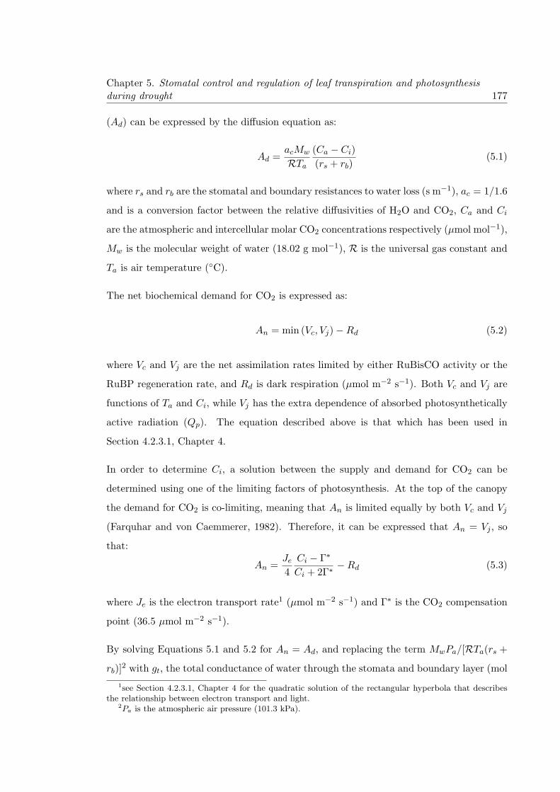
Chapter 5. Stomatal control and regulation of leaf transpiration and photosynthesisduring drought 177
(Ad) can be expressed by the diffusion equation as:
Ad =acMw
RTa
(Ca − Ci)
(rs + rb)(5.1)
where rs and rb are the stomatal and boundary resistances to water loss (s m−1), ac = 1/1.6
and is a conversion factor between the relative diffusivities of H2O and CO2, Ca and Ci
are the atmospheric and intercellular molar CO2 concentrations respectively (μmol mol−1),
Mw is the molecular weight of water (18.02 g mol−1), R is the universal gas constant and
Ta is air temperature (◦C).
The net biochemical demand for CO2 is expressed as:
An = min (Vc, Vj)−Rd (5.2)
where Vc and Vj are the net assimilation rates limited by either RuBisCO activity or the
RuBP regeneration rate, and Rd is dark respiration (μmol m−2 s−1). Both Vc and Vj are
functions of Ta and Ci, while Vj has the extra dependence of absorbed photosynthetically
active radiation (Qp). The equation described above is that which has been used in
Section 4.2.3.1, Chapter 4.
In order to determine Ci, a solution between the supply and demand for CO2 can be
determined using one of the limiting factors of photosynthesis. At the top of the canopy
the demand for CO2 is co-limiting, meaning that An is limited equally by both Vc and Vj
(Farquhar and von Caemmerer, 1982). Therefore, it can be expressed that An = Vj , so
that:
An =Je4
Ci − Γ∗
Ci + 2Γ∗ −Rd (5.3)
where Je is the electron transport rate1 (μmol m−2 s−1) and Γ∗ is the CO2 compensation
point (36.5 μmol m−2 s−1).
By solving Equations 5.1 and 5.2 for An = Ad, and replacing the term MwPa/[RTa(rs +
rb)]2 with gt, the total conductance of water through the stomata and boundary layer (mol
1see Section 4.2.3.1, Chapter 4 for the quadratic solution of the rectangular hyperbola that describesthe relationship between electron transport and light.
2Pa is the atmospheric air pressure (101.3 kPa).

Chapter 5. Stomatal control and regulation of leaf transpiration and photosynthesisduring drought 178
m−2 s−1), the balanced equation can be written as:
Je4
Ci − Γ∗
Ci + 2Γ∗ −Rd − gt(Ca − Ci) = 0 (5.4)
and so a quadratic solution for Ci can be determined:
Ci =b−√
b2 − 4ac
2a(5.5)
where a = 4gt
b = 4gt(Ca − 2Γ∗)− ac(Je + 4Rd)
c = Γ∗(8acRd − 8gtCa − acJe)
5.2.1.2 Hydrologic framework
An Ohm’s law analogue is used to describe the flow of water from the soil to the roots,
to the leaf and to the atmosphere. The flow of water is controlled by a gradient of water
potential (Ψw), which is defined by the difference in Ψw at the start (soil) and the end of the
pathway (air). This gradient is equal to the rate of water flow and the hydraulic resistance
along this pathway. Therefore, the flow of water over time along the SPA pathway can be
described as:dE
dt=
1
R
dΨ
dt(5.6)
where dΨ is the potential difference along the pathway (MPa), R is the total hydraulic
resistance along the pathway (MPa m2 s mol−1) and E is the rate of water flowing along
the pathway (mol m−2 s−1). Equation 5.6 can be used to describe the flow of water from
the soil to the leaf, and from the leaf to the atmosphere. The supply of H2O from the soil
to the leaves (Jw) is described by:
Jw =Ψs −Ψl − ρwg h
Rsoil +Rroot +Rplant(5.7)
where Ψs and Ψl are the soil and leaf water potentials respectively (MPa), the term ρwg h
describes the gravitational pull on the transport of water up through the xylem, where ρw

Chapter 5. Stomatal control and regulation of leaf transpiration and photosynthesisduring drought 179
is the density of water (0.001 MPa m−1), g is the gravitational constant (9.807 m2 s−1)and
h is the height of the plant (m), Rroot and Rplant are the hydraulic resistances from the
soil to the roots, and the roots to the leaves respectively (MPa m2 s mol−1). Lastly, Rsoil
is the soil hydraulic resistance and is a function of the hydraulic conductivity of the soil
and the root density (Tardieu and Simonneau, 1998), and can be described as:
Rsoil =ln(x2root/r
2root)
4πK(θs)(5.8)
where xroot is the mean distance between roots (m), rroot is the fine root radius (m) and
K(θs) is the hydraulic conductivity dependent on the water content of the soil (m2 MPa−1
s−1).
The evaporative demand for H2O from the leaf surface (Et) is similarly described as:
Et =Mw
RTa
(es − ea)
(rs + rb)(5.9)
where es and ea are the vapour pressures at saturation and in the air respectively (kPa)
and rs and rb are the resistances3 to water transport through the stomata and boundary
layer respectively (s m−1).4
The Ψl that equates to these levels for the supply and demand of water, can be calculated
by combining Equations 5.7 and 5.9, assuming that Et = Jw, such that:
E =Ψs −Ψl − ρwg h
Rsoil +Rroot +Rplant=
Mw
RTa
(es − ea)
(rs + rb)(5.11)
and can be simplified by again considering the term MwPa/[RTa(rs + rb)] as the total
conductance of water through the stomata and boundary layer (gt, mol m−2 s−1), Dv =
3Upper and lower case R has been used to distinguish between resistances along the soil-leaf pathway,and at the leaf.
4Though mentioned here for the sake of readability, the model uses the Penman-Monteith equation tocalculate the evaporate demand for H2O, so that the Et is described as:
Et =ΔRn + ρacpDv/rbλ[Δ + γ(1 + rs/rb)]
(5.10)
where Rn is the net radiation absorbed by the leaf (W m−2), Δ is the slope of the relationship between thesaturation vapour pressure and temperature (kPa ◦C−1), ρa is the density or air (1.204 kg m−3 @ 20◦C ),cp is the specific heat of air (1.013 MJ kg−1 ◦C−1), γ is the psychometric constant (0.066 kPa ◦C−1) andλ is the latent heat of vaporisation (2.39 MJ kg−1).

Chapter 5. Stomatal control and regulation of leaf transpiration and photosynthesisduring drought 180
(es − ea), and the sum of Rsoil + Rroot + Rplant, as the total above and below ground
resistance (Ra,b). Equation 5.11 can then be rearranged in terms of Ψl as:
Ψl = Ψs − ρwg h− gtDv Ra,b (5.12)
However, the above formulation is not exact, as there is some water stored within the plant
tissue and this stored amount can be expended before the plant uses water located in the
soil water stores. This creates a time-lag between evaporative demand for water and the
flow of water through the plant (dE), such that for an instantaneous time-step Jw �= Et
and can be described as:
dE
dt= Jw − Et
=Ψs −Ψl − ρwg h
Ra,b− gtDv
=Ψs −Ψl − ρwg h− gtDvRa,b
Ra,b(5.13)
This lag can however be incorporated into the above circuit analogue by considering the
water stored in plant as a capacitor. Leaf capacitance (Cl) is described as:
Cl =dE
dΨ(5.14)
where Cl is the leaf capacitance (mol MPa−1 m−2). Equations 5.13 and 5.14 are then
combined such that:
CldΨ
dt=
Ψs −Ψl − ρwg h− gtDvRa,b
Ra,b(5.15)
and therefore the change in Ψl over time can be described as:
dΨ
dt=
Ψs −Ψl − ρwg h− gtDvRa,b
ClRa,b(5.16)
The above equation may be solved numerically, and allows a feedback between the soil
water status and evaporative demand. Figure 5.1 shows a representation of the hydraulic
framework, including resistance to water flow and capacitance for storage of water in the
canopy, along the SPA pathway.
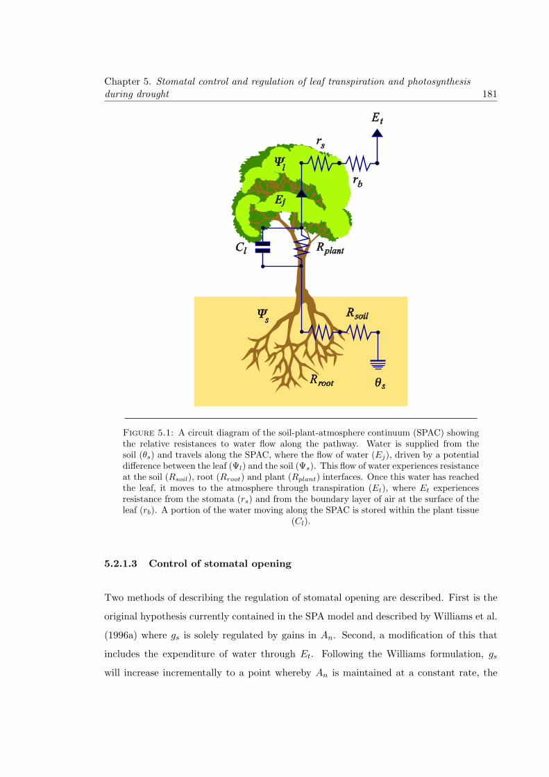
Chapter 5. Stomatal control and regulation of leaf transpiration and photosynthesisduring drought 181
Figure 5.1: A circuit diagram of the soil-plant-atmosphere continuum (SPAC) showingthe relative resistances to water flow along the pathway. Water is supplied from thesoil (θs) and travels along the SPAC, where the flow of water (Ej), driven by a potentialdifference between the leaf (Ψl) and the soil (Ψs). This flow of water experiences resistanceat the soil (Rsoil), root (Rroot) and plant (Rplant) interfaces. Once this water has reachedthe leaf, it moves to the atmosphere through transpiration (Et), where Et experiencesresistance from the stomata (rs) and from the boundary layer of air at the surface of theleaf (rb). A portion of the water moving along the SPAC is stored within the plant tissue
(Cl).
5.2.1.3 Control of stomatal opening
Two methods of describing the regulation of stomatal opening are described. First is the
original hypothesis currently contained in the SPA model and described by Williams et al.
(1996a) where gs is solely regulated by gains in An. Second, a modification of this that
includes the expenditure of water through Et. Following the Williams formulation, gs
will increase incrementally to a point whereby An is maintained at a constant rate, the

Chapter 5. Stomatal control and regulation of leaf transpiration and photosynthesisduring drought 182
operating point (ιop) can be described as:
ιop =δAn
δgs=
An(gs,i)
An(gs,i−1)(5.17)
where δ describes an infinitesimal increase in gs and An, which is equivalent to the ratio of
An between increments, i, in gs. Assuming adequate levels of irradiance and evaporative
demand, both gs and An will operate at a level around ιop. However, there needs to be some
feedback between the leaf and the demand for water by the atmosphere. Equation 5.17
describes a system where gs is increased until such a point that no appreciable increases in
An is gained. While this may be a reasonable approximation, any increases in gs will result
in appreciable increases in Et, which at the level defined by ιop may be excessive. Therefore,
I propose that An must include a weighting term defined by Et, such that increments in
gs is constrained not by an operating point, but by a cost of water parameter (λcw). This
new constraint may be defined as:
λcw =δAn/δgsδEt/δgs
=δAn
δEt
=An(gs,i)Et(gs,i−1)
Et(gs,i)An(gs,i−1)(5.18)
which is functionally equivalent to the principle of optimality described by Cowan and
Farquhar (1977). λcw can be seen as a cost parameter and allows An to be maximised
while Et is minimised, which results in a constant of carbon gained per water transpired.
The two schemes of stomatal optimisation however, are constrained by leaf water status
or Ψl, such that An and Et will remain constant while there is a sufficient supply water
to maintain the levels demanded by the atmosphere, without inducing a Ψw that is too
low and thereby inducing a reduction in gs. Thus, in the absence of stomatal regulation,
Ψl may drop to values that fall below a critical threshold, such that embolism will occur
in the xylem preventing further water flow along the SPA pathway (Eamus et al., 2006b).
Therefore, regulation of gs needs to be quantified and this effect is incorporated into
the model by the introduction of a critical threshold; the minimum leaf water potential

Chapter 5. Stomatal control and regulation of leaf transpiration and photosynthesisduring drought 183
(Ψl,min). The consequence of this is that gs and An will be maximised and Et minimised
as long as Ψl > Ψl,min holds. If Ψl is equal to, or less than Ψlmin, then no further increase
in gs will occur representing the prevention of xylem embolism.
The new model framework proposed in this study is therefore described by the following.
Using Equations 5.1 and 5.2 to describe the supply and demand for CO2, and Equations
5.7 and 5.9 to describe the respective supply and demand for H2O, while the conditions
hold that δAn/δgs > ιop for gs Model 1 or δAn/δgs < λcwδEt/δgs for gs Model 2 and
Ψl + dΨl/dt > Ψl min, determined from Equation 5.16, then the coupled leaf biochemical
and hydrologic framework that operates on the above constraints can be represented as:
⎛⎜⎜⎜⎜⎜⎜⎜⎜⎜⎝
An,1 · · · An,N
Et,1 · · · Et,N
gs,1 · · · gs,N...
...
Ψl,1 · · · Ψl,N
⎞⎟⎟⎟⎟⎟⎟⎟⎟⎟⎠
= fSPA
⎛⎜⎜⎜⎜⎜⎜⎜⎜⎜⎝
Qp,1 Dv,1 Ta,1
Qp,2 Dv,2 Ta,2
Qp,3 Dv,3 Ta,3
......
...
Qp,N Dv,N Ta,N
⎞⎟⎟⎟⎟⎟⎟⎟⎟⎟⎠
while
⎧⎪⎪⎪⎪⎪⎪⎪⎪⎪⎪⎪⎪⎪⎪⎪⎪⎪⎪⎪⎨⎪⎪⎪⎪⎪⎪⎪⎪⎪⎪⎪⎪⎪⎪⎪⎪⎪⎪⎪⎩
if gs Scheme 1
δAn
δgs> ιop
Ψl > Ψl min
if gs Scheme 2
δAn
δgs< λcw
δEt
δgs
Ψl > Ψl min
where meteorological inputs (i.e Qp, Dv, Ta, etc) are passed to the SPA model, fSPA, which
uses either stomatal conductance model 1 or 2 to determine outputs of leaf gas-exchange
(i.e. An, Et, gs, etc ). While the respective conditions hold for the stomata to remain
open, the leaf sub-models work iteratively in determining the gas-exchange variables and
can be describe by the following procedure,
1. Increment gs at a step size of ≈ 0.001 mol m−2 s−1
2. Determine Ci from Equation 5.5
3. Determine An from Equation 5.2
4. Determine Et from Equation 5.9
5. DeterminedΨl
dtfrom Equation 5.16

Chapter 5. Stomatal control and regulation of leaf transpiration and photosynthesisduring drought 184
6. Return to 1.
A caveat of the model framework described here is that it will operate in an isohydric
manner, so that gs, An, Et and Ci will operate at a constant rate irrespective of a decrease
in Ψl unless it falls below Ψl,min, at which point limitations in gs and hence An and Et
are seen.
5.2.2 Modelling approach
The two hypotheses on stomatal regulation described above in a leaf gas-exchange frame-
work were tested for a hypothetical system that is subject to increasing water stress over a
30 day period. This methodology is similar to that which was undertaken by Tuzet et al.
(2003). The system modelled was defined to represent a typical Australian native forest
that is predominantly occupied by Eucalypt species.
Meteorological forcing on the system over the 30 day period was provided by a synthetic
data-set constructed of 24 hr cycles of solar radiation (Rs), Dv and Ta (Figure 5.2). The
diurnal course of these drivers is an idealised representation of the meteorological forcing
exerted upon a forest canopy under conditions absent of rainfall and cloud cover for a
temperate, Eucalypt woodland in eastern Australia during late September (Zeppel et al.,
2008a). The diurnal course of Rs is symmetric around the midday peak, with a maximum
value occurring at 900 W m−2, with sunrise and sunset occurring at 5 am and 7 pm respec-
tively. The diurnal course of Ta ranges between 12-24 ◦C over the day, and consequently
Dv is peaks at 2.0 kPa at 2 pm. Both Ta and Dv track the course of daily irradiance but
experience a lag of approximately 2 hours. Wind speed (U) was set to be constantly high
at 8 m s−1 over the 30 day period, reducing the boundary layer resistance (rb → 0) and
defining all water lost from the plant to be directly regulated by gs, and therefore for all
equations mentioned above, it holds that gt = gs in this study. Although the meteorologi-
cal conditions are low compared to peak summer values (Zeppel et al., 2008a), I wished to
limit the effects of high Dv, so that the Ψl did not reach Ψlmin at the start of the 30 day
simulation period. However, the effects of high Dv are explored in a sensitivity analysis.

Chapter 5. Stomatal control and regulation of leaf transpiration and photosynthesisduring drought 185
Figure 5.2: Diurnal course of solar radiation (Rs), vapour pressure deficit (Dv), airtemperature (Ta) and wind speed (U) used in the simulation to test both leaf gas-exchangemodels. The diurnal course of these drivers are repeated over the 30 day simulation period.
Leaf biochemical parameters were chosen to reflect vegetation operating under the above
idealised conditions, operating on a simple soil profile (Table 5.1). Simulations were per-
formed for a 9 m tall tree with a LAI of 3 m2 m−2 distributed evenly over 10 canopy layers.
A low Rplant of 150 MPa m2 mmol−1 and low Ψlmin of -3.0 MPa was selected to allow
a period where θs is non-limiting. The soil profile for this simulation was set to be 2 m
deep, with roots having access down to a 1 m depth. The distribution of roots through the
profile was exponential and fine root radius was selected to be 0.1 mm. Root biomass was
set low at 3 kg m3 in order to provide a reasonable feedback for below ground resistance
in the system. The particle size distribution (PSD) of the profile was set as a sandy loam
(65% Clay, 10% Sand), and the initial water content of the soil (θs) was set as saturated
(0.18 m3 m−3). These values have not been selected to represent a specific site, but were
selected to test the coupling of gs with CO2 exchange by the leaves and the flow of water
through the SPAC within the SPA model.
Two representations of stomatal regulation were modelled for a 30 day drying-out period.

Chapter 5. Stomatal control and regulation of leaf transpiration and photosynthesisduring drought 186
Table 5.1: Parameters used to describe the system’s vegetation and soil profile. Param-eter descriptions, symbols, units and values are given for the 30 day simulation period.
Description Symbol Units Value
Canopy height h m 9.0Leaf area index LAI m2 m−2 2.0Foliar nitrogen Nf gN m−2 3.0Whole leaf capacitance Cl mol m−2 MPa−1 5.0Whole plant resistance Rplant MPa m2 mmol−1 150Maximum electron transport rate Jmax μmol m−2 s−1 160Maximum RuBisCO activity Vcmax μmol m−2 s−1 80Minimum leaf water potential Ψlmin MPa -3.0Operating point for stomatal efficiency ιop % 0.07Carbon gained per unit water lost λcw μmol CO2 mol−1 H2O 75
Soil depth dsoil m 2.0Rooting depth droot m 1.0Root biomass mroot kg biomass m−2 3.0Fine root radius rroot mm 0.1Whole root resistance Rroot MPa m2 mmol−1 400Sand particle size distribution S% % 65.0Clay particle size distribution C% % 10.0
The first representation (Scheme 1) is expressed by Equation 5.17, where gs is maximised to
maximise An (Williams et al., 1996a). The second representation (Scheme 2) is expressed
by Equation 5.18, where gs is maximised to maximise An while minimising Et (Cowan,
1977). Both of these schemes contain the additional constraint that represents a fail-safe
in the hydraulic system, such that gs may only be maximised to a point where Ψl remains
larger than Ψlmin. The point where gs is said to maximise An (ιop for Scheme 1 and λcw
for Scheme 2) were chosen to emulate similar daily maximums of gs on day 1. Because
this study is purely theoretical and is not specified to a particular site, it was not possible
to quantify the value of ιop with λcw; although a method for site-specific parameterisation
has been offered in Chapter 4. However, the relative effects of changing the magnitude of
these parameters has been explored in a sensitivity analysis.

Chapter 5. Stomatal control and regulation of leaf transpiration and photosynthesisduring drought 187
5.3 Results
5.3.1 Time-series of decreasing leaf and soil water potential and its im-
pact on leaf gas-exchange
Schemes 1 and 2 were applied to an idealised site (Figure 5.2) for a 30 day period, where
limiting soil water conditions were introduced. Figure 5.3 shows the effect of decreasing
Ψs on modelled leaf gas-exchange produced by the respective schemes. Both schemes
simulated similar below-ground water balances over the 30 day period, with soil water
storage gradually declining from 360 to 264 mm (Figure 5.3a) in Scheme 1 and 360 to
262 mm (Figure 5.3b) in Scheme 2. Initial daily minimums of Ψl were slightly lower in
Scheme 1 (−2.7 MPa; Figure 5.3c) than in Scheme 2 (−2.5 MPa; Figure 5.3d), which
caused Scheme 1 to reach Ψlmin much sooner during the simulation period. However, this
did not have a large impact on leaf gas-exchange over the simulation period.
Both schemes showed that while Ψs remained above -0.25 MPa, Ψl remained above Ψlmin
and Rsoil remained low and constant at 3.0 MPa m2 s mmol−1. Consequently, soil water
was not limiting on gas-exchange under these conditions and gs, An, Et and Ci operated
maximally and were symmetric around 12-noon peak (Figure 5.3e-l). However, while both
schemes displayed similar daily maximums of gs, An and Ci/Ca, the daily maximum Et
was larger in Scheme 1 (360 W m−2) than in Scheme 2 (315 W m−2). For Scheme 1, the
period where θs was non-limiting lasted approximately 11 days, while for Scheme 2 it was
longer, lasting 15 days. Once Ψs fell below −0.25 MPa, θs started to become limiting
on the system; Ψl began to reach Ψlmin and Rsoil increased slowly (3.0 → 4.0 MPa m2
s mmol−1). The decrease in Ψs over this period, which resulted in Ψl reaching Ψlmin
caused an increasing asymmetry to occur in the diurnal courses of the leaf gas-exchange
quantities. Diurnal gs in both schemes displayed distinct mid-morning and afternoon
peaks (Figure 5.3e,f), while An remain relatively unaffected (Figure 5.3g,h), Et became
asymmetric and dropped in its daily maximum values (Figure 5.3i,j) and Ci/Ca showed an
increasing drop in the afternoon (Figure 5.3k,l). For Scheme 1, this period lasted 7 days,
while in Scheme 2 this period was shorter, lasting 4 days. After Ψs fell below −0.8 MPa,
θs began to reach critical levels (for this soil type; 0.08 m3 m−3) and water stress became

Chapter 5. Stomatal control and regulation of leaf transpiration and photosynthesisduring drought 188
more evident and severe. As a result, Ψl reached Ψlmin for all daylight hours during this
period and Rsoil increased rapidly; in Scheme 1, this increase was from 4.0 to 29.0 MPa
m2 s mmol−1, while in Scheme 2, the increase was smaller, moving from 4.0 to 20.0 MPa
m2 s mmol−1. The decline in value of the gas-exchange quantities was similar for both
schemes, however daily maximum gs in Scheme 2 remained constant despite the significant
drop in θs. For Scheme 1, the period of water stress lasted for 12 days, and for Scheme
2 the period lasted 11 days. By day 30, the rooting zone of the soil had dried out and
gas-exchange had become severely limited.
5.3.2 Diurnal course of leaf gas-exchange in the two schemes
While gas-exchange showed a similar decline in both schemes over the 30 day period, there
were differences in the shape and degree of asymmetry in the diurnal responses for some of
the gas-exchange quantities. The most notable, was the difference in magnitude of daily
maximum Et that was observable between schemes at the start of the simulation period.
Additionally Scheme 2 displayed an initial asymmetry in gs that was independent of θs and
was not seen in Scheme 1. Because these disparities observed among schemes relates to
differences in stomatal regulation, a selection of days over the 30 day period were analysed
in more detail.
Figure 5.4 shows the modelled diurnal course of gs, An, Et and Ci/Ca for days 1, 14, 18,
21, 26 and 30, demonstrating the effects of declining Ψs in Schemes 1 and 2. On day
1, under non-limiting soil water conditions, all variables in Scheme 1 were symmetrical
around noon, tracing the diurnal course of Rs (Figure 5.4a-d). Scheme 2 showed similar
symmetry for An and Et (Figure 5.4f,g), but not for gs and Ci/Ca, which were asymmetric
even though θs was non-limiting (Figure 5.4e,h). This initial asymmetry in gs was in
response to increasing Dv and Ta in the afternoon and was independent of soil water
status. The effect of high afternoon Dv and Ta was not observable in Scheme 1 as a result
of poor coupling between gs and Dv. The initial asymmetry seen in Ci/Ca is the result of
the auto-correlation between gs and Ci in Equation 5.1, such that gs ∝ Ci. From day 14
onwards, both schemes displayed an asymmetry in the diurnal patterns of the gas-exchange
quantities as a result of Ψl = Ψlmin and became more pronounced as Ψs decreased. This

Chapter
5.Stomatalcontro
landregu
latio
noflea
ftra
nspira
tionandphotosyn
thesis
durin
gdrought
189
Figure 5.3: Simulated gas-exchange and soil water dynamics of Schemes 1 and 2 over the 30 day drying period. Shown above is the timecourse of (a-b) soil water storage, plant (Rplant) and soil (Rsoil) resistance, as well as (c-d) the leaf (Ψl) and soil (Ψs) water potentials,and the minimum leaf water potential (Ψlmin). Estimates of leaf gas-exchange quantities are given along this trace for (e-f) stomatalconductance (gs), (g-h) net assimilation rate (An), (i-j) latent energy (λEt) and (k-l) the ratio of intercellular and atmospheric CO2
(Ci/Ca). The dotted maroon lines and the change in colour (blue to light blue), denote the transition from well-watered to water-stressedconditions. Modelled An and Et have been multiplied by LAI to scale from leaf to canopy.

Chapter 5. Stomatal control and regulation of leaf transpiration and photosynthesisduring drought 190
resulted in morning and afternoon peaks in the diurnal course of gs and An, an initial
morning peak and then decline in Et, and an increasing draw-down of Ci in the afternoon
as a consequence of the stomata beginning to regulate Ψl as water supply declined. The
asymmetry in these quantities was the result of the reduced ability of soil to supply water
to the canopy, due to a decrease in hydraulic conductivity and increase in Rsoil.
In Scheme 1, the decrease in Ψl caused a decline in gs after it had reached a midday peak at
approximately 12-noon, falling to a minimum at 2 pm when Ψl = Ψlmin. As the soil dried
out, the peak in gs occurred earlier in the morning, and decreased from 0.32 to 0.22 mol
m−1 s−1 (days 1 and 30 respectively) as a result of Ψl reaching Ψlmin sooner (Figure 5.4a).
In contrast to this, An remained unresponsive to declining gs until Ψs was less than -0.8
MPa (day 18 onwards), when the system became severely water stressed (Figure 5.4b).
During this period An began to display increasing asymmetry that was coupled with the
large draw-down in Ci/Ca and the increase in Rsoil (Figure 5.3a). With the decline in Ψs,
the diurnal course of Et showed a distinct morning peak that then declined to a constant
for the remaining daylight hours. Despite Ψl reaching Ψlmin, Et did not experience a
midday depression due to increasing Dv in the afternoon which counteracted the drop in
gs (Figure 5.3c). The draw-down of Ci/Ca increased with the progression of the drought
and followed the increase in daily Dv and Ta and was limited by Ψl = Ψlmin (Figure 5.3d).
The increased draw-down was correlated with the midday depression in gs.
Scheme 2 displayed an initial asymmetry in gs under high Ψs, with a maximum gs occurring
at 8 am, which then decreased over the course of the day with increasing Dv and Ta and
was limited by Ψl = Ψlmin (Figure 5.3e). Morning peak gs did not move in time, due to
the effect of increasing Dv on gs in the early morning, which was not yet limited by Ψl
reaching Ψl,min. As a result, daily maximum gs (0.32 mol m−1 s−1) did not decrease over
the 30 day period despite decreasing Ψs and did not display a midday depression until
day 18. Compared to Scheme 1, the afternoon peaks of gs in Scheme 2 were of a lower
magnitude due to a stronger coupling between gs andDv. The response of An to decreasing
Ψs was similar to Scheme 1, with the exception that Scheme 2 displayed deeper midday
depressions in An and had slightly higher afternoon peaks (Figure 5.3f). Like Scheme 1, An
was insensitive to gs, but was sensitive to increasing Rsoil and decreasing Ci/Ca. Scheme
2 Et displayed a similar diurnal response to Scheme 1, although an asymmetry in the

Chapter 5. Stomatal control and regulation of leaf transpiration and photosynthesisduring drought 191
Figure 5.4: Diurnal course of leaf gas-exchange variables for days 1, 14, 18, 22, 26 and30 during the 30 day drying period. Show above are (a) stomatal conductance (gs), (b)net assimilation rate (An), (c) latent energy (λEt) and (d) the ratio of intercellular andatmospheric CO2 (Ci/Ca) in Scheme 1, and (e) gs, (f) An, (g) λEt and (h) Ci/Ca inScheme 2. The red line denotes gas-exchange that is operating under non-limiting soilwater conditions. Modelled An and Et has been multiplied by LAI to scale from leaf to
canopy.

Chapter 5. Stomatal control and regulation of leaf transpiration and photosynthesisduring drought 192
diurnal response was not observed until a later period (day 18 instead of 14). However, by
day 30 the Et of each scheme was at a very similar level (Figure 5.3g). There was a much
smoother draw-down in Ci/Ca for Scheme 2 than Scheme 1, and the initial asymmetry
of Ci/Ca was evident under non-limiting θs (Figure 5.3h). As was observed in Scheme 1,
Ci/Ca was correlated with gs in Scheme 2.
5.3.3 Relationships among leaf gas-exchange quantities
5.3.3.1 Between leaf gas-exchange quantities and environmental drivers
The relationships between leaf gas-exchange and the environmental drivers of Rs and Dv
are shown in Figure 5.5 for Schemes 1 and 2, where days 1, 18, 22, 25 and 30 show the
effects of progressive soil drying on these relationships. All quantities show a hysteresis
loop in response to the diurnal changes in Rs and Dv, as well as the difference of pre-dawn
leaf water potentials (Ψlpd) between days.
For Scheme 1, the relationship between gs, Dv and Rs remains proportional under well-
watered conditions. The response of gs to Rs was positive, and highly correlated, display-
ing a tight hysteresis loop and showing that gs retained a strong relationship with light
throughout the day (Figure 5.5a). In contrast to this, the response to Dv showed a much
weaker relationship and was less correlated, with the major effects of Dv on gs limited to
the afternoon (Figure 5.5b). In Scheme 2, the relationship between gs and Rs was also
positive, with the exception that towards midday a slight, negative relationship developed
in response to increasing Dv (Figure 5.5c). This relationship was also less strongly cor-
related than in Scheme 1, displaying a larger degree of hysteresis. Scheme 2 exhibited
a negative relationship of gs with Dv during the morning compared with a positive one
observed in Scheme 1 (Figure 5.5d). Thus gs in Scheme 2 was more sensitive to Dv than
in Scheme 1.
Little difference was observable between Schemes 1 and 2 for the responses of An, Et and
the Ci/Ca ratio to Dv and Rs. Any differences that arose were in part due to Scheme 2
regulating Et and exhibiting a smaller decline in Ψs. An and Et were highly correlated
with Rs, with increasing hysteresis in the relationships occurring as the soil dried out.

Chapter
5.Stomatalcontro
landregu
latio
noflea
ftra
nspira
tionandphotosyn
thesis
durin
gdrought
193Figure 5.5: Shows the responses of Scheme 1 and 2 (a-d) stomatal conductance (gs), (e-h) net assimilation rate (An), (i-l) latent energy(λEt) and (m-p) the ratio of intercellular and atmospheric CO2 (Ci/Ca), against solar radiation (Rs) and vapour pressure deficit (Dv)
respectively. Relationships between these quantities are shown over the 30 day drying period for days 1, 18, 22, 25 and 30.

Chapter 5. Stomatal control and regulation of leaf transpiration and photosynthesisduring drought 194
This caused An and Et to become increasingly insensitive to Rs in the afternoon (Fig-
ure 5.5e,g,i,k). The relationships between An, Et and Dv were positive under non-limiting
soil water conditions, but displayed a large hysteresis. As the soil dried out, this hys-
teresis decreased, but the quantities An and Et became increasingly insensitive to Dv for
most of the day (Figure 5.5f,h,j,l). The opposite was seen for the Ci/Ca ratio, which was
largely insensitive to Rs and Dv and displayed very little (for Dv) or no hysteresis (for Rs)
under well watered conditions (Figure 5.5m-p). However, as soil water became limiting,
hysteresis increased and the negative relationship became stronger.
For all quantities in both schemes, the effects of increasing soil water-stress caused gs, An,
Et and the Ci/Ca ratio to become increasingly insensitive to Rs and Dv. In response to
increasing Dv, the relationship with gas-exchange became increasingly, negatively corre-
lated due to declining Ψs. The poor correlation and large hysteresis between gas-exchange
and Dv under well-watered conditions is largely the result of a 2 hr time-lag that occurs
between Rs and Dv, such that all quantities are initially out of synchronisation with Dv re-
gardless of water status. For instance, gs reaches a maximum at 12-noon while Dv reaches
a maximum at 2 pm. The opposite effect was seen with Rs, with the relationship collapsing
in response to the shift of daily maximum gs from the midday mark (in synchronisation
with daily maximum Rs) to earlier in the morning; creating an asymmetry in the diurnal
course (Figure 5.4). This in turn was a consequence of tighter stomatal regulation as Dv
increased under the conditions of decreasing Ψl.
5.3.3.2 Between stomatal conductance, assimilation and transpiration
Relationships between gs, An and Et are presented in Figure 5.6 for Schemes 1 and 2,
using the same set of days representing the drying period mentioned in the last section.
In Scheme 1, under non-limiting soil water conditions, the relationship between gs and
An was highly and positively correlated, such that An ∝ gs (Figure 5.6a). As the soil
dried out, there was an increasing draw-down in CO2 during the afternoon, following an
increase in Dv in the afternoon and Ψl reaching Ψlmin. This created a lag between An and
gs, which caused a disproportionality between these quantities and increased the degree of
hysteresis as Ψs declined. This process similarly occurred in Scheme 2, with the exception

Chapter 5. Stomatal control and regulation of leaf transpiration and photosynthesisduring drought 195
that the relationship was less correlated, due to a greater sensitivity of gs to Dv and
resulted in an initial hysteresis (Figure 5.6b). There was a positive and highly correlated
relationship between gs and Et in Scheme 1 (Figure 5.6c). Declining Ψs resulted in a Ψl
reaching Ψlmin and a decrease in the slope of the relationship between gs and Et. This
caused Et to become increasingly insensitive to gs over the drying period. These patterns
were similarly seen in Scheme 2, with the exception of an initial, large hysteresis that
existed under well-watered conditions and was the results of a greater sensitivity to Dv
(Figure 5.6d). This large hysteresis showed an insensitivity of Et to increasing gs during
the early morning, which expanded to the rest of the day as the soil dried out.
Figure 5.6: Plotted relationships between (a-b) stomatal conductance (gs) and netassimilation rate (An), as well as (c-d) gs and latent energy (λEt) for Schemes 1 and 2respectively. The effects of soil drying on these relationships is shown for a selection of
days (1, 18, 22, 25 and 29) during the 30 day drying period.

Chapter 5. Stomatal control and regulation of leaf transpiration and photosynthesisduring drought 196
5.3.3.3 Between leaf water potential, assimilation and transpiration
Figure 5.7: Plotted relationships between (a-b) leaf water potential (Ψl) and net as-similation rate (An), as well as (c-d) Ψl and latent energy (λEt) for Schemes 1 and 2respectively. The effects of soil drying on these relationships is shown for a selection of
days (1, 18, 22, 25 and 29) during the 30 day drying period.
Figure 5.7 shows the sensitivity of An and Et to decreasing Ψl for Schemes 1 and 2 over
the 30 day drying period. Selected days showing these relationships are the same as
those used in the last two sections. In Scheme 1, An was negatively correlated with Ψl
and displayed initial hysteresis, where morning An was less sensitive to Ψl than in the
afternoon (Figure 5.7a). With the decrease in Ψs, the relationship shifted towards Ψlmin
as Ψlpd decreased. This caused an increase in hysteresis and the correlation between An
and Ψl to decrease. Scheme 2 displayed a similar pattern to Scheme 1, however, there
was a lesser degree of hysteresis and An was slightly more sensitive to Ψl in the morning
(Figure 5.7b). A highly negative relationship existed between Et and Ψl for Schemes 1

Chapter 5. Stomatal control and regulation of leaf transpiration and photosynthesisduring drought 197
and 2 (Figure 5.7c,d), where Et was highly sensitive to Ψl in both morning and afternoon.
As the soil dried out and Ψl began to reach Ψlmin, Et and Ψl became less correlated and
the relationship slightly less negative. Scheme 1 had a higher maximum Et and a Ψlpd
that decreased much faster than in Scheme 2.
5.3.4 Sensitivity analysis
5.3.4.1 Sensitivity of gas-exchange to stomatal efficiency and the cost of water
Figure 5.8 shows the effect of changing the stomatal efficiency in Scheme 1, and cost of
water in Scheme 2 on the daily mean values of modelled leaf gas-exchange. For convenience,
both ιop and λcw are denoted as the operating points (OP) for the respective schemes from
this point on. The OPs were selected to cover the possible upper and lower limits; for
Scheme 1 the range for ιop was 0.3, 0.7, 0.2, 0.5 and 1.0 %, and for Scheme 2 the range for
λcw was 30, 75, 150, 300 and 500 μmol mol−1.
Variation in the value of OP in each scheme caused the initial values of the gas-exchange
quantities to vary. In both schemes, increasing the OP increased the number of days for
which the system was not limited by θs. The length of this period was the result of the
initial values of mean diurnal stomatal conductance (gs), transpiration rate (Et) and the
daily minimum of the ratio between intercellular and atmospheric CO2 (Ci,min/Ca) having
different magnitudes on day 1. However, increasing the OP showed very little effect on
the initial values of mean diurnal net assimilation rate (An). At the start of the 30 day
drying period, gs was found to be the most sensitive to variation in OP. In Scheme 1,
increasing ιop (0.03 → 1.00 %) caused initial gs to decrease from 0.35 to 0.07 mol m−2 s−1
(Figure 5.8a), while in Scheme 2, increasing λcw (30 → 500 μmol mol−1) caused initial gs
to decrease from 0.32 to 0.09 mol m−2 s−1 (Figure 5.8b). Initial Et was also sensitive to
variation in the OP. In Scheme 1, increasing ιop resulted in a decrease in initial Et from
253 to 119 W m−2 (Figure 5.8c), while in Scheme 2, increasing λcw resulted in a similar
decrease in initial Et from 236 to 126 W m−2 (Figure 5.8d). Increasing the OP had very
little effect on the initial values of An, with increases in ιop and λcw resulting in very small
decreases of 19.7 to 18.2 μmol m−2 s−1 in Scheme 1 (Figure 5.8e) and 19.7 to 18.5 μmol

Chapter 5. Stomatal control and regulation of leaf transpiration and photosynthesisduring drought 198
Figure 5.8: Sensitivity of daily mean (a) stomatal conductance (gs), (b) latent energy(λEt), (c) net assimilation rate (An) and (d) the daily minimum ratio between intercellularand atmospheric CO2 (Ci,min/Ca) to stomatal efficiency (ιop = 0.03, 0.07, 0.2, 0.5 and1.0 %) in Scheme 1, and (e) gs, (f) λEt, (g) An and (h) Ci,min/Ca to the cost of water(λcw = 30, 75, 150, 300 and 500 μmol m−2 s−1) in Scheme 2. A run using the defaultoperating points is given in red, while changes in ιop and λcw are given in shades of blue.

Chapter 5. Stomatal control and regulation of leaf transpiration and photosynthesisduring drought 199
m−2 s−1 in Scheme 2 (Figure 5.8f). Variation in OP had moderate effect on the starting
values of Ci,min/Ca. In Scheme 1, the effect of increasing ιop resulted in a decrease of initial
Ci,min/Ca from 0.91 to 0.72 (Figure 5.8g), while in Scheme 2, increasing λcw resulted in a
decrease from 0.90 to 0.70 (Figure 5.8h).
High initial values of gs and Et resulted in a faster depletion of soil water over the 30
day period, and therefore, little to no gas-exchange by day 30. Values of Et, An and
Ci,min/Ca decreased substantially when θs became limiting and a low OP was selected.
However, variation in the OP did not have a great effect on gs for the same conditions,
as it converged towards similar values at the end of the drying period (Figure 5.8a-b).
This was observed in the small difference of OP derived values of gs on day 30, where the
difference in Schemes 1 and 2 were both 0.02 mol m−2 s−1. For Et, a higher initial value
dictated a larger decline in water-use over the drying period (Figure 5.8c-d). In Scheme 1,
a low OP caused Et to decrease from 253 to 20 W m−2 over the 30 day period, where θs
became limiting on day 6. In Scheme 2 the decline in Et over the same period was from
236 to 25 W m−2, where θs became limiting on day 10. However, a high OP allowed both
schemes to maintain a constant Et (119 and 126 W m−2 for Schemes 1 and 2 respectively)
over the drought, such that θs never became limiting on the system. Despite having little
effect on An at the start of the drought, variation in the OP had a large impact on the
final values of An (Figure 5.8e-f). In Scheme 1, a low OP caused a decline from 19.7 to
6.7 μmol m−2 s−1 over the 30 days, while in Scheme 2 this decline was from 19.7 to 6.3
μmol m−2 s−1. However, a high OP allowed An to remain relatively unchanged over the
drought in both schemes (19.7 μmol m−2 s−1 over 30 days). Similar to the effects seen on
Et, a lower OP caused Ci,min/Ca to decline at a faster rate (Figure 5.8g-h). In Scheme 1,
this resulted in a decline from 0.91 to 0.20 over the 30 days, while in Scheme 2 the decline
was from 0.90 to 0.18. As was observed with the other gas-exchange quantities, a high OP
allowed Ci,min/Ca to be maintained at a constant rate over the drought. Although this was
predominantly true for both schemes, Scheme 2 experienced a minor drop in Ci,min/Ca of
0.70 to 0.67 on the last day. Although this may be a numerical error in the model due to
the extreme water-stressed conditions.
The effect on the total carbon gained and water lost over the period in both schemes is
shown in Figure 5.9. The most significant result of varying the system OP was its impact

Chapter 5. Stomatal control and regulation of leaf transpiration and photosynthesisduring drought 200
Figure 5.9: The sensitivity of (a-b) soil water potential (Ψs), (c-d) cumulative car-bon gain and (e-f) cumulative water loss to variation in stomatal efficiency (ιop =0.3, 0.7, 0.2, 0.5 and 1.0 %) in Scheme 1 and the cost of water (λcw = 30, 75, 150, 300and 500 μmol mol−1) in Scheme 2. A run using default operating points is given in red,
while changes in ιop and λcw are given in shades of blue.
on the rate of soil water depletion during the simulation period (Figure 5.9a-b). A high
OP resulted in smaller rate of decline in Ψs in Schemes 1 and 2 (-0.05 to -0.68 MPa), while
a low OP resulted in a large decline in Ψs (-0.05 to -1.82 MPa). This resulted in large
differences in the total amount of water lost by the end of the drying period (Figure 5.9c-
d). In Scheme 1, a low ιop (0.03%) resulted in a total water-use of 0.090 m3 m−2, while
a high ιop (1.00%) resulted in a total water-use of 0.066 m3 m−2. Similar totals were
observed for Scheme 2, with low and high λcw values (30 and 500 μmol mol−1) resulting
in water-use totals of 0.089 and 0.70 m3 m−2 respectively. However despite the large
differences in total water-used, very little difference was observed between total carbon
gained for different OP values (Figure 5.9e-f). In Scheme 1, the difference in total carbon
gained for low and high ιop was 142 and 153 gC m−2 respectively, while for Scheme 2 this

Chapter 5. Stomatal control and regulation of leaf transpiration and photosynthesisduring drought 201
difference for low and high λcw was 141 and 155 gC m−2 respectively. These results show
that there is no great benefit in maintaining a high gs to marginally increase An, as this
results in an excessive increase in Et. This can be expressed by comparing the water-use
efficiencies (WUE) for the low and high OPs, where the WUE is defined as total carbon
gained divided by total water-use (A/E). In Scheme 1, a low ιop has a WUE of 1.53 gC
m−3 H2O, while a high ιop has a WUE of 2.33 gC m−3 H2O. Similarly, in Scheme 2, a low
λcw has a WUE of 1.57 gC m−3 H2O and a high λcw has a WUE of 2.22 gC m−3 H2O.
Although a low OP may be reasonable during well-watered conditions, a high OP is more
desirable in maintaining high levels of carbon gain while minimising water loss during a
drought period.
5.3.4.2 Sensitivity of gas-exchange to vapour pressure deficit
Figure 5.10 shows the effect of increasing daily maximum vapour pressure deficit (Dv,max)
on gas-exchange in each scheme. A range of Dv,max (1.0, 2.0, 3.0, 4.0, 5.0 and 6.0 kPa) was
selected to show the effects of a high and low evaporative demand that may be forced upon
these systems. The most obvious result of changing Dv,max was the change in the initial
values of gs and Et, and the length of time the system was not limited by θs. In Scheme 1,
a high Dv,max (6.0 kPa) caused the system to become water-limited immediately on day 1,
while a low Dv,max (1.0 kPa) prolonged the point of drying out until day 20. For Scheme
2 under a high Dv,max, soil water did not become a limiting factor until day 4, while a low
Dv,max similarly extended the non-limiting period to day 20. This showed that Scheme 2
was able to maintain a longer period where θs was not limiting to gas-exchange as Dv,max
increased and was the result of a greater coupling to Dv that allowed better regulation of
Et.
In Scheme 1, initial gs under non-limiting θs, remained high and declined from 0.27 to
0.13 mol m−2 s−1 when Dv,max increased from 1.0 to 6.0 kPa (Figure 5.10a). In Scheme 2,
gs was more sensitive to variation in Dv,max, with initial high values of 0.29 mol m−2 s−1
declining substantially to 0.10 mol m−2 s−1 as Dv,max increased (Figure 5.10b). In both
schemes, for Dv,max ≥ 2.0 kPa, gs → 0 as water-stress became more severe. Variation in
Dv,max produced the most significant change in initial Et for Scheme 1, with a decline of

Chapter 5. Stomatal control and regulation of leaf transpiration and photosynthesisduring drought 202
Figure 5.10: Sensitivity of daily mean (a-b) stomatal conductance (gs), (c-d) latentenergy (λEt), (e-f) net assimilation rate (An) and (g-h) the daily minimum ratio betweenintercellular and atmospheric CO2 (Ci,min/Ca) to variation in daily maximum vapourpressure deficit (Dv,max) for Schemes 1 and 2 respectively. The values of Dv,max thatwere simulated are 1.0, 3.0, 4.0, 5.0 and 6.0 kPa, given in shades of blue, while the default
Dv,max of 2.0 kPa is given in red.

Chapter 5. Stomatal control and regulation of leaf transpiration and photosynthesisduring drought 203
388 to 170 W m−2 with the increase in Dv,max (Figure 5.10c). In Scheme 2, initial Et was
lower at 1.0 kPa and experienced a smaller decline from 285 to 174 W m−2 (Figure 5.10d).
For Dv,max > 2.0 kPa, Et → 0 as the drought progressed. Variation in An with increasing
Dv,max between schemes did not differ significantly, with initial range in An for low and
high Dvmax decreasing from 19.76 to 18.54 μmol m−2 s−1 (Figure 5.10e-f). However,
increasing evaporative demand largely affected An in the late drying period, with values
declining to 2.53 to 2.06 μmol m−2 s−1 in Schemes 1 and 2 respectively under 6.0 kPa,
while operating under a Dv,max = 1.0kPa, An decreased to only 14.36 to 15.90 μmol m−2
s−1. Increasing Dv,max had a moderate effect on Ci,min/Ca and little difference in this
response could be observed between schemes. An increase in Dv,max from 1.0 to 6.0 kPa
resulted in a moderate decline in initial Ci,min/Ca from 0.91 to 0.68 (Figure 5.10g-h) and
these values converged towards 0.19 by day 30. The more pronounced reduction in gs
that occurred in Scheme 2 was a result of a greater coupling with Dv. Scheme 1, although
displaying some reduction in gs, contained no such feedback and changed little in its initial
values despite a larger evaporative demand. For Scheme 1, an increase in Dv,max did not
impede gs maximising towards ιop, but rather increased the amount of water lost from the
canopy and resulted in Ψl reaching Ψlmin much sooner. Scheme 2 showed a much higher
sensitivity to Dv and therefore displayed a tighter regulation of Et.
The effect of varying Dv,max on total carbon gained and water lost over the period for
both schemes is shown in Figure 5.11. A low Dv,max resulted in Ψs declining at a much
smaller rate due to a low Et, where it declined from -0.05 MPa on day 1 to -2.02 MPa in
Scheme 1 (Figure 5.11a) and -1.94 MPa in Scheme 2 (Figure 5.11b) by day 30. Although
this affected water-use during the middle of the drying period, this did not result in a large
difference between period totals of water-use at high and low Dv,max. In Scheme 1, period
total water use at a Dv,max of 1.0 kPa was 0.084 m3 m−2 and at a Dv,max of 6.0 kPa was
increased to 0.089 m3 m−2 (Figure 5.11c). In Scheme 2, increasing Dv,max from 1.0 to 6.0
kPa increased period total of water-use from 0.085 to 0.088 m3 m−2 (Figure 5.11d). While
different Dv,max values produced similar water-use totals, there was a more noticeable
difference in period totals of carbon gain. A large Dv,max resulted in a lower carbon
gained at the end of the 30 day drought, where Scheme 1 was showed a Dv,max of 1.0 kPa
resulted in a carbon gain of 161 gC m−2 and when increased to 6.0 kPa, this resulted in a

Chapter 5. Stomatal control and regulation of leaf transpiration and photosynthesisduring drought 204
decrease in carbon gain at 107 gC m−2 (Figure 5.11e). This was similarly seen in Scheme
2, with increasing Dv,max from 1.0 to 6.0 kPa resulting in total carbon gain declining from
162 gC m−2 to 115 gC m−2 (Figure 5.11f). These results were framed in terms of a scheme
WUE at low and high Dv,max. For Scheme 1, a Dv,max of 1.0 kPa produced a WUE of
1.92 gC m−3 H2O and increasing Dv,max to 6.0 KPa decreased WUE to 1.20 gC m−3 H2O.
Similarly, in Scheme 2, increasing Dv,max from 1.0 to 6.0 kPa decreased WUE from 1.88
down to 1.31 gC m3 H2O. This showed that while Schemes 1 had a higher WUE under
low Dv, when Dv was increased Scheme 2 retained a higher WUE.
Figure 5.11: The sensitivity of (a-b) soil water potential (Ψs), (c-d) cumulative carbongain and (e-f) cumulative water loss to variation in in daily maximum vapour pressuredeficit (Dv,max) for Schemes 1 and 2 respectively. The values of Dv,max that were simu-lated are 1.0, 3.0, 4.0, 5.0 and 6.0 kPa, given in shades of blue, while the default Dv,max
of 2.0 kPa is given in red.

Chapter 5. Stomatal control and regulation of leaf transpiration and photosynthesisduring drought 205
5.4 Discussion
5.4.1 Performance of the SPA model using two descriptions of stomatal
regulation
The aim of this study was to investigate the simulated process of leaf gas-exchange (par-
ticularly gs) in the SPA model as it operates under drought. This involved simulating
two schemes of leaf-gas exchange for a canopy operating under idealised environmental
conditions and subjected to a 30 day drying period. The strategies of stomatal regulation
tested in this work were defined by two schemes; (i) the maximisation of gs to maximise An
(Williams et al., 1996a) and (ii) the maximisation of An while Et is minimised (Cowan and
Farquhar, 1977). When soil water conditions were non-limiting, both schemes increased
stomata aperture in order to increase carbon uptake. The point at which stomatal opening
was maximised was defined by two respective operating points; ιop for Scheme 1 and λcw
for Scheme 2. The effect of water stress due to decreasing Ψs was reflected by the condition
that gs is limited (and therefore An and Et) when Ψl = Ψlmin. Under non-limiting θs,
Scheme 1 increased gs until An was maximised, regardless of Et. However, this process is
not totally true as there must be some feedback between gs and Et which is sensitive to
variations in Dv. The reasoning behind Scheme 2 was to include this feedback by necessi-
tating that An be balanced with Et. This increased the sensitivity of gs and Et to Dv and
allowed gs to be maximised so long as the canopy did not excessively transpire water in
order to gain insignificant amounts of carbon. The consequences of this new strategy was
a change in the diurnal response of gs under well-watered conditions, which was defined
by a reduction in daily maximum stomatal conductance (gsmax) and a distinct asymmetry
(rather than symmetry) around noon in response to increasing evaporative demand as the
day progressed. This resulted in a reduced Et, which in turn resulted in a prolonged period
where θs was not limiting to leaf gas-exchange. Additionally, Scheme 2 was more WUE
than Scheme 1 under soil water-stress and when subjected to increases in daily evaporative
demand.
The results of Scheme 1 and 2, compare well with the studies of Makela et al. (1996) and
Tuzet et al. (2003), which use similar modelling exercises to simulate leaf gas-exchange

Chapter 5. Stomatal control and regulation of leaf transpiration and photosynthesisduring drought 206
over drought. The results given by Schemes 1 and 2 show similar reductions in An, Et and
Ci/Ca in response to decreasing soil water availability (Makela et al., 1996; Tuzet et al.,
2003). However, there are differences in the diurnal response of gs between these studies.
In Tuzet et al. (2003), the diurnal response of gs is a symmetric pattern around noon,
with a weak effect of increasing Dv and Ta, and this agrees with the daily response of gs
described by Scheme 1. In contrast, Makela et al. (1996) shows the diurnal course of gs
to be similar to that produced by Scheme 2, which has a stronger coupling between gs,
Dv and Et. These differences may be due to different modelling approaches in estimating
leaf gas-exchange. Tuzet et al. use the semi-empirical BBL model to determine gs, An
and Et, while Makela et al. use the Cowan-Farquhar hypothesis to determine these same
quantities. The BBL assumes an a priori functional response of gs to Dv, whereas the
Cowan-Farquhar hypothesis assumes that excessive Et induces stomatal closure. This is
why there is difference in the diurnal response of gs between the studies mentioned above
and between both schemes used in this study. The choice of which of these two diurnal
stomata responses is true, constitutes to how stomata respond to soil water deficits and
raises the question of whether gs is regulated by Ψl or by Et at the evaporating sites of the
stomata (Tyree and Sperry, 1988; Monteith, 1995; Eamus and Shanahan, 2002; Leuning
et al., 2003). Additionally, there is also the question of what operating point should canopies
function at, so as to benefit their productivity, while conserving water supplies (Makela
et al., 1996; Thomas et al., 1999a,b; Schymanski et al., 2008b; Katul et al., 2010). These
questions are now discussed below in the proceeding sections.
5.4.2 Response of stomata to transpiration and vapour pressure deficit
The diffusion of water vapour through the leaf stomata is described by Et = gsDv, which
shows a direct relationship between the quantities of Et, gs and Dv. For a low range
of Dv (0.0 − 2.0 kPa), Et increases asymptotically. However, as Dv increases further
(2.0− 7.0 kPa), Et declines in response to decreasing Ψl (Prior and Eamus, 1999; Eamus
and Shanahan, 2002; Zeppel et al., 2004). The response of gs and Et for a large range of
Dv is characterised in the three-phase response as described by Monteith (1995), where
gs and Et operate under three distinct regimes that describe the regulatory role of leaf
stomata in preventing excessive water loss. While the three-phase response was observed

Chapter 5. Stomatal control and regulation of leaf transpiration and photosynthesisduring drought 207
in Scheme 2, it was not in Scheme 1. The asymptotic increase in gs with increasing Dv
as displayed by Scheme 1 under non-limiting θs, did not follow the relationship that have
been observed in other studies (Oren et al., 1999; Oren and Pataki, 2001; Pataki and Oren,
2003; Ewers et al., 2007). This relationship did not conform to the expected exponential
decay of gs to increasing Dv until θs became limiting and so any decline was likely the
result of declining Ψl. In contrast to this, Scheme 2 displayed the expected exponential
decline in gs with increasing Dv under non-limiting θs. Additionally, Scheme 2 gave a clear
representation of the three-phase response, showing the movement through regimes A, B
and C as described by Monteith (1995), and observed by Thomas and Eamus (1999) and
Eamus and Shanahan (2002). This is further supported by Oren et al. (1999), who have
shown that all three regimes exist under well watered conditions, with a collapse of regime
A (gs decreases linearly with increasing Et) as θs decreases. This response is also similar
to the relationships shown by Oren and Pataki (2001); Misson et al. (2004); Uddling et al.
(2005). While Scheme 1 shows some presence of regimes B and C, regime A appears to
be only slightly present when the canopy was water-stressed. However, this response is
similar to that found by Tuzet et al. (2003), whose model uses Ψl to regulate gs under
declining Ψs.
5.4.3 Response of assimilation to stomatal conductance and transpira-
tion
There was an evident lag between gs, Et and An over the drought period, where modelled
gs had reached low values, yet still produced substantial values of An. This was the result
of the increasing draw-down of Ci/Ca as the canopy became increasingly water-stressed,
such that An became dampened by declining gs in the late drying period. Although this
effect is expected and has been observed in the field (Schulze, 1986; Sage, 1994; Prior et al.,
1997; Lawlor and Cornic, 2002) and produced by other models (Makela et al., 1996; Tuzet
et al., 2003; Schymanski et al., 2007). This was also reflected in the sensitivity analysis,
which showed that despite varying the OP or Dv,max to create large differences in initial
gs, An remained relatively unchanged. Again this is likely the result of declining Ci/Ca
which dampens the proportionality between gs and An. However, this explanation should
be taken with caution, as initial Ci/Ca during the simulation of both schemes was higher

Chapter 5. Stomatal control and regulation of leaf transpiration and photosynthesisduring drought 208
than observed in other studies (Fordyce et al., 1997; Prior et al., 1997; Eamus et al., 1999).
Although the above argument offers a reasonable explanation for the lag and insensitivity
between these quantities, there may still be a problem in the coupling between gs and
An in the SPA model, as some trial runs that were numerically unstable still produced
reasonable values of An.
5.4.4 The level of stomatal efficiency and the cost of water
A large problem in this study was in defining the values of the OPs (ιop and λcw). The
problem with Equations 5.17 and 5.18 is that their respective OPs are abstract unless
parameterised against field data (Hari et al., 1986; Makela et al., 1996; Katul et al., 2010).
If set incorrectly, this can result in the loss of copious amounts of water to gain only an
infinitesimal amount of carbon, or conversely, results in very little water lost and so even
less carbon gained (Williams et al., 1996a; Misson et al., 2004). In Chapter 4, a possible
method in quantifying the level of ιop was presented, and the same method should be
equally applicable in quantifying λcw. However, the aim of this chapter was to explore two
alternative schemes of declining gs. Therefore, it was beyond the scope of this work to
optimise these two OPs. If leaf-gas exchange is not limited by soil water availability, then
the plant will maximise its productivity and so the OP can be relatively high. However
the same OP under water-limited conditions would no longer be valid and should decrease
with decreasing θs. The consequence of this feedback not being incorporated into SPA is
that daily gs,max remains disproportionate to θs despite the forcing that should be applied
by severe water stress; in Scheme 1, gsmax is seen to remain fairly high (Figure 5.4c), while
in Scheme 2 it is constant (Figure 5.4c). Although it is not expected that gsmax would drop
significantly with decreasing θs, there should be some decline nevertheless. The reasoning
behind a constant gsmax occurring throughout the drought in Scheme 2, is because for this
time of day Rs is high,and Dv low and Ψl > Ψl,min, such that gs is able to increase to
such a high value. Makela et al. (1996) were able to solve this problem using the model of
Hari et al. (1986), whereby their cost of water parameter (a function of the initial θs and
probability of rainfall) changed under increased soil drying. A similar method linking the
level of θs to the OP, possibly through some monotonic function, could be incorporated
into SPA to solve this problem.

Chapter 5. Stomatal control and regulation of leaf transpiration and photosynthesisduring drought 209
5.4.5 Effects of leaf water potential on gas-exchange
The stomatal control of leaf-gas exchange is a direct function of Et, Dv and Ψl, all of which
fluctuate over a daily time-course. In the absence of available energy (light) to evaporate
water, leaf stomata remain shut and there is very little evaporative demand for water by the
atmosphere. Before dawn, water is in equilibrium along the soil-root-leaf pathway (that is
all plant cells are roughly saturated with water), so that Ψlpd ≈ Ψs (Eamus et al., 2006b).
As the sun rises, light levels and temperature increase and stomata open so as to assimilate
CO2, and will continue to open their stomata to maximise An (Williams et al., 1996a).
Consequently, Et increases and so Ψl decreases. The level to which Ψl decreases, and
its impact on leaf gas-exchange will differ depending on whether the plant is ioshydric or
anisohydric in behaviour (Tardieu and Simonneau, 1998; Jarvis and Davies, 1998; Schultz,
2003). The SPA model contains the feedback of Ψl on gas-exchange described above, such
that gas-exchange will remain unimpeded so long as conditions remain above that which
causes xylem embolism to occur. This allows the model to keep gs, Et and An at maximised
rates until further reductions in Ψs cause the condition Ψl = Ψlmin. The mechanism in
both schemes can be related to isohydric behaviour, such that if water is available, then
the plant will spend it regardless of depleting water availability so long as Ψl remains
above Ψlmin. Modelled leaf gas-exchange in SPA is therefore operating on an on or off
switch, with no long-term regulation by the available water supply unless it begins to lead
to catastrophic failure of the plant’s hydrology.
Despite the improvement offered by Scheme 2, the SPA model only considers leaves to
operate in an isohydric manner, due to the constraint of Ψlmin. Such that modelled gs
does not decline with Ψl, but is only limited when Ψl = Ψlmin. There should therefore be
some monotonic penalty function on gs that is applied before the condition of Ψl = Ψlmin is
met. Tuzet et al. (2003) use a model that similarly incorporates a feedback between Ψl and
Ψs to regulate stomata aperture. However, (ignoring structural differences of the model
itself), Ψl tends to regulate gas-exchange through a monotonic cost function, where the
decrease in Ψl, due to decreasing Ψs places a penalty on leaf gas-exchange. Additionally,
their calculation of the water potentials along the SPA pathway is also more robust, as it
incorporates the effects of root water potential (Ψr); an important factor in considering

Chapter 5. Stomatal control and regulation of leaf transpiration and photosynthesisduring drought 210
the drying-out of the soil around the root-zone as the day progresses (and then to be re-
saturated at night as stomata close and Ψl drops). Equation 5.12 and 5.16 relate directly
to the Ψs itself, which is affected on a daily time-course not an hourly one, and so the
effects of soil drying will be delayed by a day, before the effects of the regulation of gs by
Ψl will be seen. The problem with incorporating this dynamic is in establishing the flow
of water from the soil to the roots, which can be done using the Richards’ flow equation.
However, this is not easily calculated, and requires a numerical solution in order to find it.
It is something that should be considered in the future development of the SPA model, as
this dynamic is important in establishing a truer measure of Ψl. Additionally, problems
in defining the absolute value of the OP as discussed above, may result in higher than
necessary gs and so will needlessly reduce Ψl to operate close to Ψlmin. Work by Tardieu
and Davies (1993) and expanded upon by Tardieu and Simonneau (1998), discusses using
chemical signalling between the roots and the leaf (via concentrations in xylem [ABA])
to penalise leaf gas-exchange under increasing water stress. Results of these studies have
shown that gs responds to xylem [ABA] concentration and Ψr rather than Ψs, and this
feedback could be incorporated into the SPA model in emulation of the work done by
Dewar (2002).
5.5 Conclusion
The SPA model was tested over a 30 day drying cycle using two different schemes that
were defined by their respective methods of regulating leaf gas-exchange. Scheme 1 was
defined as a plant that increased its leaf stomatal aperture to maximise carbon uptake,
so long as soil water was not limiting. Scheme 2 defined the increase in stomata aperture
to maximise carbon uptake while minimising the water lost from the leaf. Meteorological
and physiological conditions for the modelled canopy were idealised, to allow the effects of
stomatal regulation to be a dominant factor in modelled gas-exchange. Under non-limiting
soil water conditions, diurnal patterns in gas-exchange were symmetric and became asym-
metric as the canopy became increasingly water stressed. Under these conditions, both
schemes performed similarly, with the exception that Scheme 2 displayed a stronger re-
sponse between stomatal conductance, transpiration and vapour pressure deficit. Stomatal

Chapter 5. Stomatal control and regulation of leaf transpiration and photosynthesisduring drought 211
conductance displayed a continual diurnal asymmetry regardless of soil water status. The
asymmetry of stomatal conductance in Scheme 2 resulted in a slower rate of depletion
of soil water over the 30 day period, allowing assimilation rates to remain maximised for
a longer period. A sensitivity analysis showed that the selection of OP is important in
determining the rate of soil water-extraction and the impact this has on the rate of assimi-
lation. Consequently a high OP in both schemes was found to be desirable in maintaining
a maximised rate of assimilation and that the λcw = δAn/δEt formulation is slightly more
effective than ιop = δAn/δgs at regulating leaf stomata under higher levels of vapour
pressure deficit.

Chapter 6
Conclusions
This thesis aimed to answer four questions that are important in the process of modelling
water and carbon fluxes from forest canopies in Australia. These questions are; (i) can
water fluxes from a canopy be estimated using a simple empirical model without the need
for canopy conductance? (ii) can a simple empirical model of canopy water-use be applied
across multiple sites without the need for site-specific calibration? (iii) can a Soil-Plant-
Atmosphere (SPA) model be used replicate canopy gas-exchange for a Australian tropical
savanna? and (iv) can the leaf gas-exchange process in the SPA model be improved so as to
maximise carbon gain while simultaneously minimising water loss from the leaf following
the Cowan and Farquhar optimality hypothesis?
The result of the work described in this thesis is a body of work that (a) involved the
development of a simple empirical model of canopy water-use; and (b) required the modi-
fication and improvement of a highly mechanistic and more complex soil-plant-atmosphere
(SPA) continuum model (Williams et al., 1996a). The development of the simple canopy
water-use model was in response to the problem of having to define surface conductance
when using the Penman-Monteith equation (Monteith, 1965) to estimate transpiration.
By removing surface conductance as a critical input, canopy water-use can be estimated
from three readily available meteorological variables. The result is a model that is broadly
applicable for many sites, and one that can be used as a tool in the management of water
resources within industries such as forestry and mining. However, in order to investigate
212

Chapter 6. Conclusions 213
the dynamics of water and carbon gas-exchange from forest canopies, and the mechanics
underlying these dynamics, a more complex SPA model was used. While the SPA model
has been successfully applied to various global ecosystems, the lack of an expression for C4
photosynthesis in the model has limited its application to tropical savannas. Modification
of the SPA model was therefore undertaken in order to improve its applicability to savan-
nas through incorporation of C4 photosynthesis. This was an important improvement to
the SPA model, as savanna ecosystems contain C4 vegetation, which contribute a large
percentage of total ecosystem productivity. Additionally, this modification and subsequent
application of the SPA model to a savanna site highlighted important issues in the leaf
gas-exchange calculations when soil water became limiting. These problems were pursued
by testing the SPA model for a simulated drought, where an improvement to modelled leaf
gas-exchange was suggested and tested. In order to encapsulate the major findings of the
work presented in this thesis, this chapter therefore provides a synthesis of the conclusions
that have been drawn from each of the previous chapters. This is followed by a range of
further questions that help to define the future direction of this research.
6.1 Modelling water fluxes from a forest canopy
Drawing from a general discussion on the important role of canopy water-use in an ecosys-
tem’s water balances (Chapter 1), models that are able to estimate water fluxes from the
land surface, through evaporation and transpiration, have an important application as
management tools in the areas of forestry, mining, and water and land resource manage-
ment (Meyer, 1999; Raupach, 2001; Zhang et al., 2001). There is, therefore, a need for a
simple canopy water-use model that is information-light (a small number of inputs that
are readily available) and have a high applicability, which can be used to determine annual
water budgets. The Penman-Monteith (PM) equation (Monteith, 1965) has been the most
robust model for determining estimates of canopy water-use of a site via readily available
inputs of meteorological data, such as solar energy, temperature, wind speed and humidity
(Granier and Loustau, 1994; Zhang et al., 1997; Harris et al., 2004; Leuning et al., 2008).
However, while the PM equation has experienced wide applicability and theoretical ap-
peal, it is hindered by its requirement for estimates of canopy conductance (gc) as a critical

Chapter 6. Conclusions 214
input to run the model. Determining gc for a site is a difficult process (Chapter 2), as
measuring it requires extensive field campaigns where stomatal conductance (gs) can be
directly measured over short-term periods (days) using a porometer and then up-scaled to
an estimate of gc through the leaf area index (LAI) (Zeppel et al., 2008b). However, the
application of the PM equation, and other canopy water-use models, are applied in the
mid-term (annual) and so field measurements of gc, although informative, are not entirely
suitable for models that run for extensive periods. There are models available that can
provide period estimates of maximum gc (i.e. Kelliher et al., 1995), but such models still
require the effects of soil water availability and a full coupling to the leaf physiology to be
considered (Wang and Leuning, 1998; Tuzet et al., 2003). The other approach is through
use of a Jarvis-Stewart (JS) model (Jarvis, 1976; Stewart, 1988) which incorporates a set
of empirical cost functions which are calibrated according to the site. This approach has
proved to be the most frequently used in the literature in overcoming the “gc problem” and
involves an inversion of the PM equation to properly calibrate the model. Although this
methodology has been successful and offers an insight into seasonal trends of gc (Granier
et al., 1996b; Zhang et al., 1997; Harris et al., 2004), the process is still rather cumbersome
and requires site-specific calibration of the model to work. Given the above difficulties in
using the PM equation, one of the primary goals of this thesis was to develop a simple
model that could be used to make short- to mid-term (annual) predictions of Ec without
the need for gc as an input.
6.1.1 Developing a simple model to estimate canopy water-use
Chapter 2 described the development and testing of a simple model of canopy water-use
that is functionally equivalent to the PM equation and was based on the empirical frame-
work of Jarvis (1976) and Stewart (1988). This empirical Ec model, called the modified
Jarvis-Stewart (MJS) model, requires only three meteorological drivers as inputs, these
being solar radiation (Rs), vapour pressure deficit (Dv), and soil water content (θs), as
well as a set of empirically determined environmental response parameters that are cali-
brated for the model. This kept with the idea of limiting the number of required input
parameters to those which are readily available and avoiding unnecessary model complex-
ity. Initial testing showed a strong capability of the MJS model to estimate Ec for a

Chapter 6. Conclusions 215
native Australian woodland, over a concatenated four month period, which encompassed
contrasting seasons (two months of summer and two months of winter) and displayed
variations in temperature, humidity and soil water availability. These results showed the
MJS model to be perform equally well as (if not better than) the PM equation, giving a
good explanation of the variation in the measured data (87%) and producing a low root
mean square error (RMSE). Model performance and robustness was further supported
through a strong comparison with a statistical benchmark, which was created using an
ANN. The high correspondence between the MJS model and the statistical benchmark
showed that Rs, Dv and θs provide adequate information to make reasonable predictions
of Ec. Further information such as temperature or wind speed did not provide an in-
crease in model performance. When applied to another four subsequent sites (Chapter 3),
estimated Ec determined from the MJS model continued to correspond well with the mea-
sured data. Not all sites were water-limited and variation in Rs and Dv was adequate
enough to explain the variation in Ec at these sites; this was further supported by the
statistical benchmarks created for each site. Using only three readily available meteoro-
logical inputs to derive accurate predictions of Ec provides a favourable alternative to the
PM equation, which requires gc as an input and does not directly consider the effects of
limiting θs. Furthermore, the MJS model is more accessible in contrast to typical land
surface-exchange models (LSM) that need twenty to forty parameters of meteorology, soil
hydraulics, leaf phenology and biochemistry information (which in itself requires extensive
parameterisation) in order to run (Chapter 4).
6.1.2 Applicability of the modified Jarvis-Stewart model
It was shown in Chapter 3 that calibration of the MJS model across five disparate sites
showed that the relationship between Ec, Rs and Dv was similar among sites. Conse-
quently, the site-specific model parameters describing these relationships were similar in
value despite differences in the species composition of the forest canopy and soil at each
site. This led to the hypothesis that it may be possible to determine reasonable estimates
of site Ec using an average set of model parameters. Calibrating the model for all five
sites simultaneously produced a set of site-average model parameters, such that the model
considers the response of Ec to variation in Rs and Dv to be the same across all sites. It

Chapter 6. Conclusions 216
was established that differences in the parameter values between the sites was likely the
result of these values varying around the site-average mean. From a numerical perspective,
it was suggested that the parameter values are being drawn from very wide distributions
(i.e. the variance of the parameter values is large), while from a biological perspective
(assuming well-watered conditions) the response of Ec was strongly linked to Dv, and this
response to Dv is similar among the five sites in study due to similar climatic conditions.
However, not all model parameters could produce an average response across sites. The
parameters describing the maximum canopy water-use (Ecmax) and soil hydraulic prop-
erties (wilting point, θw and critical point, θc) still need to be determined specifically for
each site, as these directly relate to factors that will vary among ecosystems (LAI and
soil type). Although these parameters could not be averaged across sites, their values can
possibly be determined from other site-specific information. For example regressions of the
model parameters against site characteristic information such as canopy basal area, LAI
and annual rainfall were positive. However, only the relationship between Ecmax and basal
area was statistically significant, LAI and rainfall were not. It must be noted, however,
that there were only five data points from which to construct these relationships. Conse-
quently, a statistically insignificant result was not surprising. If the model were applied
to a further number of sites (say ten), thereby increasing the range of values, then a more
confident conclusion could be drawn on linking site characteristics with Ecmax.
Application of the model with both site-specific and site-average parameter sets showed
that despite some variation among parameter values, estimates of site Ec were highly
comparable. Furthermore, applying the model to a site without initial calibration, will
result in only a slight decrease in performance; at least for this set of sites (Chapter 3).
Considering that the MJS model (using site-average parameters) was capable of producing
reasonable estimates of site canopy water-use, this then reduces the required inputs to the
model. In the case of sites that are limited by θs the number of model parameters reduces
from seven to three , and for sites that are not limited by θs, the number of parameters
reduces from five to one. The result is that the end user requires only the necessary
meteorological inputs (Rs, Dv and θs), and information on the maximum rate of water-
use for the site and soil water characteristics; information which can be proscribed from
potential evaporation and the Saxton equations (Saxton and Rawls, 2006) respectively.

Chapter 6. Conclusions 217
This offers a very useful management tool for water resource management in the industries
of forestry, mining and land management, which are unlikely to undertake extensive field
campaigns to determine information on leaf-level characteristics, root distributions and
canopy phenology that is needed to run more complex LSMs.
6.2 Modelling canopy gas-exchange using a Soil-Plant-
Atmosphere model
While the MJS model is a simple model able to provide estimates of canopy water-use, it
has a greater applicability as a management tool than a research one, as it does not provide
a detailed mechanistic understanding of forest canopy processes. Furthermore, it does not
model carbon fluxes from forest canopies. The SPA model on the other hand, is able to
provide reasonably accurate estimates of water and carbon fluxes from a canopy, as it is
built upon a mechanistic understanding of canopy gas-exchange. The SPA model requires
an extensively detailed parameterisation of a site in order to replicate the processes of gas-
exchange, soil water balance and light interception correctly (Chapter 4). While models
such as SPA have a large requirement of information, once the model is parameterised for
a site, it can then be used to investigate processes that may not be possible in the field or
ask detailed questions about the system. For example, “What is the impact on the canopy
if we increase the average daily maximum temperature?” However, there are limits to the
SPA model, and this thesis has attempted to overcome two of these limitations.
6.2.1 Investigating savanna canopy and water fluxes
The SPA model has been successfully applied over a number of disparate ecosystems.
However, while successful, the application of this model has only considered ecosystems
that are comprised entirely of C3 vegetation. Because only C3 photosynthesis is considered
by the model, this prevents its application to tropical savannas, which contain a significant
component of C4 vegetation. Furthermore, this limits the SPA model as research tool, as
tropical savannas are an important global biome that contributes approximately 26-30%
of global gross primary productivity (GPP) (IPCC, 2007). Considering that C4 vegetation

Chapter 6. Conclusions 218
is a major component of global landscapes, the lack of a C4 photosynthesis model severely
limits the application of SPA in global climate models. There are a number of important
characteristics of a savanna that distinguishes it from other ecosystems, (i) the canopy
understorey is dominated by tall C4 grasses which make an almost equal contribution to
total ecosystem productivity, (ii) savannas exist in areas that experience highly seasonal
rainfall (distinct wet and dry seasons) and so the C4 grasses are only active during the
wet season when there is a high water content in the upper soil profile. This seasonality
in rainfall results in a seasonality in GPP and evapotranspiration (ET) The work outlined
in Chapter 4 therefore described the modifications to the leaf-level processes of the SPA
model that were needed to simulate the above characteristics, such that it could accurately
replicate a tropical savanna located in northern Australia. In order to define the first
(and major) characteristic of a savanna in the SPA model, two C4 photosynthesis models
were tested and incorporated. These were a simplified C4 photosynthesis model (Collatz
et al., 1992) and a more complex, mechanistic C4 photosynthesis model (von Caemmerer
and Furbank, 1999). Of these two models, the simple model was selected to describe
C4 vegetation in SPA, because it was less complex (requiring less leaf-scale information
to work) and performed as well as the more detailed mechanistic model. To define the
second savanna characteristic (the senescent nature of the savanna grasses), the model
was further modified to incorporate a dynamic distribution of canopy leaf area. That is,
the distribution of leaf area through the canopy was allowed to change on a daily basis
rather than being constant throughout the year. The result was that the C4 grass layers
could be described as active during the wet season and inactive in the dry season, thereby
capturing their senescent habit in the dry season.
Following a detailed parameterisation of the site, which included details of the leaf bio-
chemistry of the C3 canopy and C4 grass and the underlying soil profile, the SPA model
was run to replicate water and carbon flux measurements derived from eddy-covariance
(EC) over five years for a tropical savanna in the northern Australia (Chapter 4). The
use of a C4 photosynthesis model to described the grass understorey improved wet season
total estimates of GPP by 13 to 15% when compared with a simulation that considers only
C3 photosynthesis. However, the choice between C3 and C4 vegetation type did not result
in any great difference in estimated ET. Consequently, having the SPA model correctly

Chapter 6. Conclusions 219
parameterised to simulate a savanna ecosystem produced two important outcomes. The
first outcome was that the C4 grass understorey was shown to contribute largely (≈48%;
564 − 575 gC m−2) to total ecosystem GPP when it was active in the wet season. This
level of contribution was almost equal to the level of productivity that was simulated for
the C3 canopy overstorey. Additionally, while the levels of productivity between the C3
trees and C4 grasses were almost equivalent, there was a great disparity in the levels of
water-use. The C4 grasses contributed much less to total savanna water-use (≈ 23%;
130− 160 mm) than the overstorey, which highlighted the water-use efficient nature (the
ratio of carbon gained to water lost) of C4 vegetation. These values, as well as the overall
simulated annual totals for the savanna compared well with totals measured with other
savannas in the literature (Miranda et al., 1997; Hanan et al., 1998). The second insight
arising from this research was that savanna ET and GPP were predominantly driven by
the seasonal variation in LAI rather than changes in θs. Partitioning the canopy according
to vegetation type showed the monthly diurnal variation in Et for the C3 trees remained
constant and high throughout the year; that is, there was no seasonal decline in Et during
the dry season despite a decline in θs. This raised the question of what was driving the
seasonality in canopy fluxes. This question was investigated by simulating two scenarios,
i) a energy-limited scenario (limited by light-interception); where LAI was allowed to vary
seasonally but θs remained constant and high, and ii) a water-limited scenario; where LAI
was held constant, but θs was allowed to vary seasonally. The results from these scenarios
showed that an abundant soil water supply in the upper soil profile did not allow ET and
GPP to remain at wet season levels during the dry season, but a high and constant LAI
throughout the year however, allowed ET and GPP to remain at wet season levels despite
a large decline in θs. This shows that savanna ET and GPP are insensitive to variation of
θs in the upper soil profile, due to the tree canopy having roots that are able to access deep
soil water stores. Past studies conducted at this site indicated similar findings (O’Grady
et al., 1999; Hutley et al., 2001; Eamus et al., 2001). Consequently, the modelled savanna
was demonstrated to be limited by light interception, such that the decrease in GPP and
ET during the dry season was driven by the seasonal decrease in total savanna LAI.

Chapter 6. Conclusions 220
6.2.2 Parameterising the stomatal efficiency
Chapter 4 also looked at the impact on the leaf gas-exchange in the SPA model with the
incorporation of the C4 photosynthesis; that is the differences in modelled An, gs and Et
between the two phenology types (C3 and C4 vegetation). The SPA model uses a unique
coupled photosynthesis-stomatal conductance model, which operates to increase gs until
net CO2 assimilation is maximised. The point at which modelled An is maximised (and
therefore the upper limit of modelled gs) is set by user-defined operating point (OP) (or
stomatal efficiency ; ιop), which is representative of all vegetation modelled. This posed
a problem, as C4 vegetation (by nature) is able to maximise An at much lower levels
of gs than C3 vegetation, due to its ability to inhibit photorespiration (von Caemmerer
and Furbank, 1999). Consequently, the OPs between these two vegetation types will be
different. It was therefore critically important that the C4 species were assigned their own
ιop, as their An will be maximised at a much lower magnitude of gs (and therefore have a
lower Et) compared with C3 species. This problem was solved by incorporating a separate
ιop for C3 and C4 vegetation in the model. Additionally, a methodology was developed
in order to parameterise ιop (for both C3 and C4 species), by calibrating SPA with the
slop of the Ball-Berry-Leuning (BBL) model (Chapter 4). This methodology required
fitting the BBL relationship to C3 and C4 leaf-scale data that had been measured for the
specific species types that were present at the site; the result being separate slopes for
C3 and C3 species. The SPA model was then used to replicate the the BBL relationship,
where the slope of this relationship is determined by the value of ιop. An ιop for both
C3 and C4 species was then determined by adjusting its magnitude in order to match
the slopes determined from the BBL model (Chapter 4). Although this methodology was
quite involved, it allowed a way to quantify a critical parameter of the SPA model without
having to calibrate the model to the data. Most importantly, however, it showed that the
relationship between gs and An for C3 and C4 species are very different. This difference
being the result of C4 vegetation being able to inhibit photorespiration and therefore be
more water-use efficient than C3 vegetation (Collatz et al., 1992; von Caemmerer and
Furbank, 1999; Ghannoum et al., 2003).

Chapter 6. Conclusions 221
6.2.3 Improving the leaf-level process in the Soil-Plant-Atmosphere
model
Estimated period and annual totals of ET made by the SPA model in Chapter 4 were
found to overestimate the measured totals of ET consistently over the five year study
period. Although this was in part due to some error in the parameterisation of the model
(i.e. whole plant conductance being higher than it should have been), it was also due
to gs, An and Et not being well coupled in the model itself. Chapter 5 explored the
sensitivity of the leaf gas-exchange sub-model in SPA to drought, with the purpose of
investigating the covariance between gs, Et and An under a declining θs. The leaf gas-
exchange scheme in the SPA model as described by Williams et al. (1996a) regulates gs
using two assumptions; (i) that the stomata regulate Et through the leaf water potential
(Ψl), and gs will be limited when Ψl reaches a critical threshold value (Ψlmin) to prevent
hydraulic failure in the xylem (Tyree and Sperry, 1988); (ii) while θs is not limiting, leaf
stomata will remain open and transpire at a rate determined by Dv in order to maximise
their carbon gain. The degree to which stomata may open is controlled by ιop, defined
as the point beyond which any increase in gs will not result in a beneficial increase in
An. While process (i) does occur in the field (e.g. Myers et al., 1997; Prior and Eamus,
1999), process (ii) fails to acknowledge that An is maximised while Et is simultaneously
minimised (Cowan, 1977). I therefore investigated a second scheme as a possible solution
to this problem. This was achieved by replacing process (ii) with the theory of Cowan
and Farquhar (1977), such that stomata aperture are regulated to maximise the balance
between An and Et; where this point is defined by a cost of water (λcw) parameter. The
schemes of Williams et al. (1996a) and Cowan and Farquhar (1977) (labelled Schemes 1
and 2 respectively in Chapter 5), were tested in the SPA model, using an idealised site,
constructed to simulate conditions of a temperate climate (indicative of a native Australian
forest) over a 30 day drying period. Consequently, this study was purely theoretical, and
provided a way of investigating improvements that could be made to the current leaf-gas
exchange framework in SPA.
The sensitivities of the gas-exchange quantities gs, Et, An and the ratio between intercellu-
lar CO2 concentration (Ci) and Ca, under both schemes were investigated under a drying

Chapter 6. Conclusions 222
regime. The results showed that the framework of Scheme 1 caused the soil profile of the
idealised site to decline in θs at a much faster rate than when using Scheme 2. Maximising
gs (and consequently increasing Et) to gain a very small increase in An in Scheme 1, re-
sulted in no net benefit to carbon uptake by the canopy. This was due to poor regulation
in the amount of water transpired as a function of the cost/benefit ratio. In contrast to
this, the framework of Scheme 2 displayed a tighter control on gs, through a greater feed-
back with Dv (and therefore Et) and consequently maintained a greater balance between
An and Et. This allowed An to operate at higher rates for a longer period during the
drought. Scheme 2 was also found to be more water-use efficient (WUE) under increasing
daily maximum Dv through a greater regulation of Et compared to Scheme 1. The results
of Scheme 1, may point to the overestimation of simulated ET observed in Chapter 4, as
gs was generally found to be too high. The magnitude of predicted gs could be reduced
through increasing the magnitude of the OP in both schemes (ιop and λcw respectively).
This also reduced the decline in θs and allowed more carbon to be gained in the long
run. However, reasons for why a canopy will operate at different ιop and λcw values were
not investigated, as it was beyond the scope of this study. It is expected however, that a
plant will assume an OP that results in the best balance between carbon gain and water
loss; that is, the magnitude of the OP represents a measure of the regulation of Et that is
occurring. Developing upon the methodology of parameterising ιop, mentioned in the last
section may also offer the best possible way of parameterising λcw.
Although Scheme 2 displayed better regulation of gs compared with Scheme 1, there were
still evident problems that need to be investigated. Both schemes were poorly coupled with
leaf water status during the drought, such that the gas-exchange quantities only became
limiting when Ψl = Ψlmin. Additionally, modelled gs was found to be poorly coupled
with modelled An and this insensitivity may be the result of the structure of the leaf level
process in SPA. Additionally, while both schemes operated in an isohydric manner, they do
not display the necessary coordination between the liquid flow of water and gs, such that
Ψl is maintained within an acceptable range (Maseda and Fernandez, 2006). Although
modifications to the current framework of SPA have provided a greater feedback between
Et, gs and Dv, these quantities still need to have a greater coupling with Ψl to better
simulate a plant under water-stress. This may be accomplished by linking changes in Ψl

Chapter 6. Conclusions 223
to changes in root water potential (Ψr) rather than Ψs (discussed in the next section).This
is critically important, as Australian forest canopies are subject to a high range of Dv and
low θs compared with other forests globally (e.g. European boreal forests).
6.3 Empirical versus process-based modelling
This thesis has primarily dealt with the development, modification and use of two specific
types of model. The empirical MJS model provided a relatively easy and successful way
of estimating canopy water fluxes (with the potential application to carbon fluxes), while
the process-based SPA model gave a more detailed estimation of both water and carbon
fluxes, as well as information on the canopy and root-soil interface process that govern
them. Generally speaking, the SPA model is the more advantageous model, as it allows
us to ask insightful scientific questions about the effects of varying forces acting upon and
within a system, as well as allowing us to simulate scenarios such as the impacts of climate
change and land-use (Macinnis-Ng et al., 2010). However, while the SPA model has the
advantage of giving a more detailed output of canopy processes, it still relies on empirical
relationships to describe important responses, such as soil hydraulic characteristics (Saxton
et al., 1986), temperature effects on the leaf (McMurtrie et al., 1992b; Massad et al., 2007)
and leaf biochemistry (McMurtrie et al., 1992a) to name a few. Consequently, for the
SPA model to work correctly, a detailed and accurate parameterisation of an ecosystem
(or site) is required. However, even this does not guarantee a model’s success, as any
measurement of model performance is spatially and temporally specific (Abramowitz et al.,
2009). In contrast, models based purely on empirical relationships, such as the MJS model,
can be much easier to apply, as they are specifically calibrated to the conditions of an
ecosystem and provide a high level of performance assuming that such conditions remain
relatively constant (Medlyn et al., 2005b; Makela et al., 2008). The disadvantage of using
such a model though is obviously seen in the limitations of site specific calibration and a
much reduced amount of output information when compared with process based models.
There is therefore no easy answer to the question of which of the two model types is
better, as both are more specific to certain purposes. Process-based models are effectively
scientific tools that can be used to ask interesting and insightful questions, with specific

Chapter 6. Conclusions 224
application to forecasting and experimental design, while conversely empirical models are
more applicable in asking questions about the data itself, having application in gap-filling
and benchmarking. It is therefore my hope that the work presented in this thesis has
shown the merits of using both types of models, and will contribute to the larger body
of work that is currently being accomplished by the international land-surface modelling
community.
6.4 Further research
The MJS model provided a successful way of estimating canopy water fluxes. Additionally,
modifications to the leaf gas-exchange framework of SPA, extended the applicability to
estimating both water and carbon fluxes to environments where C4 is a major component
of the vegetation. Enumerated below are ideas for further research into modelling canopy
water and carbon fluxes.
6.4.1 Future applications of the MJS model
1. To further the applicability of the MJS model, it would be ideal to test the model for
ecosystems that experience a different climate to Australia. Additionally, it would
also be valuable to see if the site-average parameter values are applicable for sites
on other continents.
2. As well as further application of the model across other ecosystems, the MJS model
should be tested with eddy-covariance and remote-sensing data. This would offer a
simple model that could be readily applied to monitor ET from land surfaces without
the need to quantify surface (stomatal) conductance.
3. Undertaking an analysis of greater depth into why average parameter values are as
statistically significant as site-parameterised values. Using Bayesian analysis, one
could investigate the distributions of each of the model parameters and compare
whether they are being drawn from the same distribution. The benefit of this is
that it would provide a robust quantification of the level of uncertainty in model
predictions (predictions within a region of confidence).

Chapter 6. Conclusions 225
4. The MJS framework could be applied to other canopy gas-exchange quantities such as
GPP or respiration. Furthermore, this would raise the question “Do these quantities
display the same responses to Rs, Dv and θs that is observed for ET?”. If so, an
average set of parameters (describing these similar responses) could be applied to
various gas-exchange quantities and allow a simple means of estimating ecosystem
gas-exchange (ET and GPP) without the need for highly complex LSMs.
6.4.2 Improvements and further testing of the SPA model
1. It would be ideal to test the robustness of SPA, with the added C4 photosynthesis
sub-model, to other savanna ecosystems, or ecosystems that have a large presence of
C4 vegetation. This would allow further assessment of the contributions of C4 plants
to carbon sequestration and provide a means of investigating the effects of climate
change on tropical savannas.
2. Currently, SPA does not have a working carbon allocation or growth component
model in its framework (that has been published). Incorporating a growth model
into the SPA framework would not only further its applicability, but also provide a
way of investigating carbon allocation that occurs in C4 vegetation.
3. A critical addition that must be made in the future is a separate rooting distribution
pattern for the understorey C4 grass layers, or for any other dominant vegetation
that is separate from the trees. Vegetation that has roots limited to the upper
1 − 2 metres of the soil profile will be subject to greater effects of soil drying than
vegetation which has deep reaching roots that are able to access deep stores of soil
water. Considering that C4 grasses play a dominant role in savanna landscapes, their
below-ground access to water stores needs to be correctly represented.
4. Following on from the above suggestion, a better a description on the flow of water
from the soil to the roots is needed in the SPA model. Because the saturated soil
around the roots dries out over a diurnal time course, there needs to be some feedback
between the water potentials of the root and the leaf, rather than just between the
soil and the leaf. The work of Tuzet et al. (2003) offer a solution to simulating this
process by use of the Richard’s flow equation. I believe the same concept can be

Chapter 6. Conclusions 226
applied to SPA quite easily. Whether or not this is numerically stable will need to
be tested.
5. The leaf gas-exchange framework of SPA, needs the incorporation of some penalty
to the stomatal efficiency and cost of water parameters when under conditions of
drought. A solution to this may be to follow the idea of Makela et al. (1996), who
were able to associate their cost of water parameter using relationships between the
probability of rainfall occurring for the current time-step and the level of the initial
θs. SPA does not consider the probability of rainfall, but a relationship could still
be drawn between the gs operating point and the magnitude of θs.

Appendix A
Expressions for light- and enzyme-
limited photosynthesis
Remembering that the diffusion rate of CO2 from the air through to the stomata is ex-
pressed as:
Ad = gs(Ci − Ca) (A.1)
we re-express Equation A.1 in terms of Ci, such that:
Ci =Ad − gsCa
gs(A.2)
The net CO2 assimilation rate limited by both RuBisCO activity and RuP2 regeneration
rate is expressed as:
An = min{Ac, Aj} −Rd (A.3)
such that there are two possible solutions that may be solved for An. Therefore, expres-
sions of An for both light and enzyme limited capacities are determined. First, the net
CO2 assimilation limited by the rate of RuP2 regeneration is determined by substituting
Equation A.2 into:
Aj =J
4
Ci − Γ∗
Ci + 2Γ∗ (A.4)
227

Appendix A. Expressions for photosynthesis 228
so that the above expression becomes:
Aj =
Je
(Ad − gsCa
gs− Γ∗
)4
(Ad − gsCa
gs+ 2Γ∗
) (A.5)
eliminating Ci as an input, reducing the number of unknown parameters. Equation A.5 is
rearranged as a quadratic expression using the assumption of that supply equals demand
(Ad = Aj):
4A2j − [4gs(Ca − 2Γ∗)− Je]Aj + gsJe(Ca + Γ∗) = 0 (A.6)
and therefore Aj is determined from the quadratic solution:
Aj =−b−√
b2 − 4ac
2a(A.7)
where a = 4
b = −4gs(Ca − 2Γ∗)− Je
c = gsJe(Ca + Γ∗)
Second, we now determine the net CO2 assimilation limited by RuBisCO activity, by
substituting Equation A.2 into:
Ac = VcmaxCi − Γ∗
Ci +Km(A.8)
so that the above expression becomes:
Ac = Vcmax
(Ad − gsCa
gs− Γ∗
)(Ad − gsCa
gs+Km
) (A.9)
eliminating Ci as an input, reducing the number of unknown parameters. Equation A.9 is
rearranged as a quadratic expression, and using the assumption of Ad = Ac:
A2c − [gs(Km + Ca) + Vcmax]Ac + gs(VcmaxΓ
∗ + gsKmCa) = 0 (A.10)
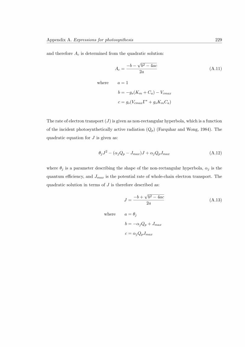
Appendix A. Expressions for photosynthesis 229
and therefore Ac is determined from the quadratic solution:
Ac =−b−√
b2 − 4ac
2a(A.11)
where a = 1
b = −gs(Km + Ca)− Vcmax
c = gs(VcmaxΓ∗ + gsKmCa)
The rate of electron transport (J) is given as non-rectangular hyperbola, which is a function
of the incident photosynthetically active radiation (Qp) (Farquhar and Wong, 1984). The
quadratic equation for J is given as:
θjJ2 − (αjQp − Jmax)J + αjQpJmax (A.12)
where θj is a parameter describing the shape of the non-rectangular hyperbola, αj is the
quantum efficiency, and Jmax is the potential rate of whole-chain electron transport. The
quadratic solution in terms of J is therefore described as:
J =−b+
√b2 − 4ac
2a(A.13)
where a = θj
b = −αjQp + Jmax
c = αjQpJmax

Appendix B
SPA stomatal model source code
B.1 Main file
Below is given the main file for running the stomatal model mentioned in Chapter 5.
PROGRAM TESTBED
! Dec lare the der ived type to be used in t h i s program
USE STOMOPT
IMPLICIT NONE
! <−−− Star t o f v a r i a b l e d e c l a r a t i o n s
! Number o f s imu la t i on s t ep s to be run
INTEGER, PARAMETER : : N=(30∗48)INTEGER : : i
! Create an array o f the type LEAFDAT, with each index pe r t a i n i ng to a
t imestep
! with s p e c i f i c met va lue s and photosynthet i c paramters
TYPE(LEAF DATA TYPE) : : l ea fC3 (N)
REAL : : CiCa , WSPD(N) , Rain (N)
230

Appendix A. Source Code 231
CHARACTER(LEN=500) : : Directory , F i l e 1 , F i l e Headers , var iab le names , &
& va r i a b l e un i t s , FMTS, FMTN
! Write the headings f o r the output v a r i a b l e s and the corre spond ing un i t s o f
measurement
var iab le names = ” Time , PAR, VPD, Ta , Ca , SWP, An, gs , Ci , Ci/Ca , Et , LWP
, Rrs”
v a r i a b l e u n i t s = ” , umol m−2 s−1, kPa , oC , umol mol−1, MPa, &
& umol m−2 s−1, mol m−2 s−1, umol mol−1, , mmol m−2 s−1, MPa, MPa
m2 s mmol”
! Format s t r i n g s
FMTS = ’ ( A, ” , ” ,A, ” , ” ,A, ” , ” ,A, ” , ” ,A, ” , ” ,A, ” , ” ,A, ” , ” ,A, ” , ” ,A, ” , ” ,A, ” , ” ,A
, ” , ” ,A, ” , ” ,A ) ’
FMTN = ’ ( F10 . 4 , ” , ” , F10 . 4 , ” , ” , F10 . 4 , ” , ” , F10 . 4 , ” , ” , F10 . 4 , ” , ” , F10 . 4 , ” , ” , &
& F10 . 4 , ” , ” , F10 . 4 , ” , ” , F10 . 4 , ” , ” , F10 . 4 , ” , ” , F10 . 4 , ” , ” , F10 . 4 , ” , ” , F10 . 4 ) ’
! <−−− End o f d e c l a r a t i o n s
! Open the f i l e that conta in s the data
F i l e 1 = ”darwin met d r i v e r s . csv ”
OPEN( UNIT=101 , FILE=Fi l e 1 , STATUS=’OLD’ )
! <−−−− Star t read ing in data
READ(101 ,∗ ) F i l e Header s
DO i =1,N
READ(101 ,∗ ) l ea fC3 ( i )%Time , l ea fC3 ( i )%Ta , l ea fC3 ( i )%Ca , WSPD( i ) , &
& lea fC3 ( i )%Rs , l ea fC3 ( i )%VPD, lea fC3 ( i )%PAR, Rain ( i ) , l ea fC3 ( i )%
SWP
ENDDO
! <−−−− End read ing in data
! Boundary l ay e r conductance (m s−1)
DO i =1,N
CALL BOUNDCOND( WSPD( i ) , l ea fC3 ( i )%Ta , l ea fC3 ( i )%gb )
ENDDO
! l ea fC3%gb = 10 .0

Appendix A. Source Code 232
l ea fC3%LAI = 2 .0 ! Doesn ’ t do anything yet
l ea fC3%Nit = 4 .0 ! Doesn ’ t do anything yet
! l ea fC3%SWP = −0.05 ! S o i l water p o t e n t i a l ( we l l watered )
l ea fC3%MINLWP = −3.5 ! Minimum l e a f water p o t e n t i a l
l ea fC3%Rp = 0.1 ! Plant hy rau l i c r e s i s t a n c e ( constant )
l ea fC3%PhoMod = 1 ! Photosynthes i s model
l ea fC3%Vcmax25 = 80 .0
l ea fC3%Jmax25 = 120 .0
l ea fC3%Vpmax25 = 0 .0
lea fC3%OptMod = 1 ! Optimisat ion model
l ea fC3%i o t a = 1.0007 ! 150 .0 <=== lambda 1.0007 <==== io t a
! l ea fC3%io t a = 250 .0
! Open the output CSV f i l e s where the va lue s w i l l be s to r ed
OPEN(UNIT=102 , FILE=”Outputs iota . csv ” , STATUS=”UNKNOWN”)
! . . . . and wr i t e the headers to go on these f i l e s
WRITE(102 ,FMTS) var iab le names
WRITE(102 ,FMTS) v a r i a b l e u n i t s
! <−−−− Run stomatal op t im i sa t i on s imu la t i on model
DO i =1,N
! Echo s imu la t i on step to the user
WRITE(∗ ,∗ ) ”Day ” , l ea fC3 ( i )%Time
! Ca l l the stomatal op t im i sa t i on model
CALL OPTIMISE STOMATA( lea fC3 ( i ) )
CiCa = lea fC3 ( i )%Ci/ lea fC3 ( i )%Ca
! Write the r e s u l t to an output f i l e
WRITE(102 ,FMTN) lea fC3 ( i )%Time , l ea fC3 ( i )%PAR, lea fC3 ( i )%VPD, lea fC3 ( i )
%Ta , l ea fC3 ( i )%Ca , l ea fC3 ( i )%SWP, &

Appendix A. Source Code 233
& lea fC3 ( i )%An, l ea fC3 ( i )%gs , l ea fC3 ( i )%Ci , CiCa , l ea fC3 ( i )%Et ,
l ea fC3 ( i )%LWP, lea fC3 ( i )%Rrs
ENDDO ! End s imu la t i on
ENDPROGRAM TESTBED
stomoptim main.f90
B.2 Leaf module
Below is the fortran code of the leaf gas-exchange module, for running the stomatal model
mentioned in Chapter 5.
MODULE STOMOPT
! FILE : stomopt im module lea f . f 90
! AUTHOR: Rhys Whitley
! DATE: August 2009
! EMAIL: Rhys . J . Whitley@uts . edu . au
!
! This i s a prototype o f the stomatal conductance opt imsat ion model us ing the
pseudo object−o r i en t ed
! des ign .
!
! This sub−model o f SPA i s now sto r ed i n s i d e the module STOMOPT and conta in s
the opera t ing paramters ,
! f un c t i on s and subrout ine s . Input in fo rmat ion such as i n t e r a c t i v e met data
and l e a f s c a l e photosynthet i c
! data i s now acce s s ed v ia a l o c a l l y dec l a r ed der ived type . The l e a f s c a l e
subrout ine s and func t i on s are
! now acce s s ed to only operate on the l e a f s c a l e data and are conta ined
with in t h i s module by po int o f the
! CONTAINS statement .
!
! Temperature f un c t i on s s t i l l need to be added to the photosynthet i c
paramters AND the ODE de r i v a t i on o f
! LWP must a l s o be inc luded .
!

Appendix A. Source Code 234
! ∗∗ This code may be added to any re formatted ve r s i on o f SPA in the fu tu r e
IMPLICIT NONE
PRIVATE ! By d e f au l t
PUBLIC : : LEAF DATA TYPE, OPTIMISE STOMATA, BOUNDCOND
! Create a der ived type f o r ho ld ing data that i s operated on by the l e a f
l e v e l
! subrout ine s and func t i on s to f i nd the optimum gs and A
TYPE : : LEAF DATA TYPE
INTEGER : : PhoMod , OptMod
REAL : : Time , PAR, APAR, Rs , VPD, Ta , Ca , gb , LAI , Nit
REAL : : MINLWP, OLDLWP, SWP, iota , Rp, Rrs
REAL : : Vcmax25 , Vpmax25 , Jmax25
REAL : : gs , An, Ad, Ci , Cm, Rd, Et , Tl , LWP
END TYPE LEAF DATA TYPE
! Parameters used in t h i s module
REAL, PARAMETER : : C3Kc25 = 310 .0 ! Ca ta l y t i c constant f o r C4 CO2
carboxy la se @ 25C
REAL, PARAMETER : : C3Ko25 = 155 .0 ! Ca ta l y t i c constant f o r C4 oxygenase @
25C
REAL, PARAMETER : : C4Kc25 = 650 .0 ! Ca ta l y t i c constant f o r C4 CO2
carboxy la se @ 25C
REAL, PARAMETER : : C4Ko25 = 400 .0 ! Ca ta l y t i c constant f o r C4 oxygenase @
25C
REAL, PARAMETER : : C4Kp25 = 80 .0 ! Ca ta l y t i c constant f o r C4 PEP
carboxy la se @ 25C
REAL, PARAMETER : : gammastar25 = 36 .5 ! CO2 compensation po int @ 25C
! S c i e n t i f i c cons tant s used in t h i s module
REAL, PARAMETER : : Pi = 3.14159
REAL, PARAMETER : : Ma = 29 .0E−3 ! Molecular mass o f a i r ( kg mol−1)
REAL, PARAMETER : : cp = 1010 .0 ! S p e c i f i c heat o f a i r ( J kg−1 K−1)

Appendix A. Source Code 235
REAL, PARAMETER : : Hd = 9.807E−3 ! Hydrual ic head
LOGICAL, PARAMETER : : TEMPON = .FALSE. ! Turn on temperature f un c t i on s
INTEGER, PARAMETER : : SoilPSD = 1 ! Choose a s o i l type [ 1=Sandy Loam ;
2=S i l t ; 3=Loam ]
!
−−−−−−−−−−−−−−−−−−−−−−−−−−−−−−−−−−−−−−−−−−−−−−−−−−−−−−−−−−−−−−−−−−−−−−−−−−−−−−−
CONTAINS
!
−−−−−−−−−−−−−−−−−−−−−−−−−−−−−−−−−−−−−−−−−−−−−−−−−−−−−−−−−−−−−−−−−−−−−−−−−−−−−−−
! Begin d e c l a r a t i o n o f subrout ine s here
SUBROUTINE OPTIMISE STOMATA( l e a f )
! Finds the opt imal stomatal conductance ( gs ) based on the cur rent weather
cond i t i ons , s un l i gh t and
! photosynthet i c parameters . The optimal gs i s then used by the subrout ine
STOMATA to f i nd the de s i r ed
! l e a f l e v e l outputs such as photosynthes i s , i n t e r n a l CO2 concentrat ion ,
r e s p i r a t i o n , l e a f temperature
! and t r an s p i r a t i o n ( water l o s s )
IMPLICIT NONE
TYPE(LEAF DATA TYPE) , INTENT(INOUT) : : l e a f
REAL : : check1 , check2 , gs low , gs h igh , t o l
!EXTERNAL ZBRENT
t o l = 1 .0E−5 ! B i s e c t i on t o l e r an c e
gs low = 1 .0E−3 ! Lower gs l im i t
g s h igh = 2 .0 ! Upper gs l im i t

Appendix A. Source Code 236
! Check i f c ond i t i on s a l low photosynthes i s , a l s o prevents night−time
stomatal conductance
! be ing c a l c u l a t ed
check1 = STOMDIFF( gs low , l e a f )
check2 = STOMDIFF( gs h igh , l e a f )
IF ( ( l e a f%PAR > 0 . 0 ) .AND. ( check1∗ check2 < 0 . 0 ) ) THEN
! Brent ’ s method to determine gs (mol m−2 s−1)
l e a f%gs = ZBRENT(STOMDIFF, l e a f , gs low , gs h igh , t o l )
CALL STOMATA( l e a f )
ELSE
! Dark c a l c u l a t i o n s − photosynthet i c c ond i t i on s poor
l e a f%gs = gs low
CALL STOMATA( l e a f )
ENDIF
END SUBROUTINE OPTIMISE STOMATA
! −−−−−−−−−−−−−−−−−−−−−−−−−−−−−−−−−−−−−−−−−−−−−−−−−−−−−−−−−−−−−−−−−−−−! −−−−−−−−−−−−−−−−−−−−−−−−−−−−−−−−−−−−−−−−−−−−−−−−−−−−−−−−−−−−−−−−−−−−
REAL FUNCTION STOMDIFF( opt gs , l e a f ) RESULT(Gsmin)
! E f f i c i e n c y check and cav i a t i on check to determine maximum gs − by t e s t i n g
whether an i o t a
! i n c r e a s e in stomatal conductance g i v e s an e f f i c i e n t i n c r e a s e in
a s s im i l a t i o n . I f FALSE,
! then gs i s s a id to be at i t s MAX fo r that time−s tep . Add i t i ona l l y i f gs can
cont inue to be
! higher , the l e a f water p o t e n t i a l goes below i t ’ s MIN, then gs i s s a id to
have reached i t s MAX.
IMPLICIT NONE
TYPE(LEAF DATA TYPE) ,INTENT(IN) : : l e a f
TYPE(LEAF DATA TYPE) : : l e a f 1 , l e a f 2
REAL,INTENT(IN) : : opt g s
REAL : : de l ta , e f f , cavchck

Appendix A. Source Code 237
! Create cop i e s o f l e a f
l e a f 1 = l e a f
l e a f 2 = l e a f
! Pre sc r ibed incrementa l change in stomatal conductance (mol m−2 s−1)
de l t a = 7 .0E−4
! Assign the gs va lue s to the l e a f c op i e s to f i nd the the r e s u l t i n g change
in An and Et
l e a f 1%gs = opt gs
l e a f 2%gs = opt gs−de l t a
! Uptake at cur rent gs
CALL STOMATA( l e a f 1 )
! Uptake at s l i g h t l y lower gs
CALL STOMATA( l e a f 2 )
! Stomata e f f i c i e n c y check
STOMOPT: IF ( l e a f 1%OptMod == 1 ) THEN
! [ dA/dgs ] : : I f e i t h e r e f f or minpsi are negat ive , then stomata i s
negat ive , stomata only open i f
! both checks are p o s i t i v e
! Maximise stomatal conductance up to i t ’ s e f f i c i e n c y po int
e f f = ( l e a f 1%An−l e a f 2%An) − ( l e a f 1%iota −1.0)
! Perform xylem cav i t a t i o n check
cavchck = l e a f 1%LWP−l e a f 1%MINLWP
! Stop opt im i sa t i on i f c av i a t i on w i l l occur
Gsmin = MIN( e f f , cavchck )
ELSE
! [ dA/dE ] : : Stomata remain open un t i l VPD becomes too high and must
c l o s e to conserve water . Balance
! i s reached between carbon−gain and water−l o s s
e f f = ( l e a f 1%An−l e a f 2%An) − l e a f 1%i o t a ∗( l e a f 1%Et−l e a f 2%Et )
! Perform xylem cav i t a t i o n check
cavchck = l e a f 1%LWP−l e a f 1%MINLWP

Appendix A. Source Code 238
! Stop opt im i sa t i on i f c av i a t i on w i l l occur
Gsmin = MIN( e f f , cavchck )
ENDIF STOMOPT
RETURN
END FUNCTION STOMDIFF
! −−−−−−−−−−−−−−−−−−−−−−−−−−−−−−−−−−−−−−−−−−−−−−−−−−−−−−−−−−−−−−−−−−−−! −−−−−−−−−−−−−−−−−−−−−−−−−−−−−−−−−−−−−−−−−−−−−−−−−−−−−−−−−−−−−−−−−−−−
SUBROUTINE STOMATA( l e a f )
! Determines l e a f l e v e l s t a b l e Ci , net a s s im i l a t i o n rate , d i f f u s i o n rate ,
mi tochondr ia l r e s p i r a t i o n ,
! l e a f temperature and l e a f evaporat ion f o r g iven gs .
IMPLICIT NONE
TYPE(LEAF DATA TYPE) ,INTENT(INOUT) : : l e a f
REAL,PARAMETER : : Pa=101.0 , t o l =1.0E−5
! Ca l cu la t e l e a f temperature based on t h i s gs
l e a f%Tl = l e a f%Ta
! Ca l cu la t e APAR
l e a f%APAR = l e a f%PAR∗( 1−exp (−0.7∗ l e a f%LAI) )
! Evaporation ra t e in mol m−2 s−1
l e a f%Et = MAX(0 . 0 , PENMANMONTEITH( l e a f%gs , l e a f%Tl , l e a f%APAR, l e a f%
VPD, l e a f%gb ) )
! l e a f%Et = l e a f%gs ∗ l e a f%VPD !/Pa
! Ca lcu la te mi tochondr ia l r e s p i r a t i o n
l e a f%Rd = 0.105∗ l e a f%Nit∗EXP(LOG(2 . 0 ) ∗( l e a f%Tl−10.0) /10 . 0 )
! Ca l cu la t e t o t a l below and above ground r e s i s t a n c e to water f low
l e a f%Rrs = HYDRORES( l e a f%SWP) ! /1000 .0
! Ca l cu la t e the l e a f water p o t e n t i a l (MPa)
l e a f%LWP = l e a f%SWP− l e a f%Et ∗1000 .0∗ ( l e a f%Rp+l e a f%Rrs )
! Ca l cu la t e a s s im i l a t i o n ra t e based on user dec l a r ed photo synthe s i s model

Appendix A. Source Code 239
PATHWAY: SELECT CASE ( l e a f%PhoMod)
! Farqhuar C3 photo synthe s i s model ( Farqhuar and Cowan , 1977)
CASE(1 )
l e a f%Ci = ZBRENT( CDIFF, l e a f , 0 . 1 , l e a f%Ca , t o l )
l e a f%An = FARQUHAR( l e a f%Vcmax25 , l e a f%Jmax25 , C3Kc25 , C3Ko25 , &
gammastar25 , l e a f%Rd, l e a f%PAR, l e a f%Tl , l e a f%Ci )
! Co l l a t z C4 photo synthe s i s model ( Co l l a t z et a l . 1992)
CASE(2 )
l e a f%Ci = ZBRENT( CDIFF, l e a f , 0 . 1 , l e a f%Ca , t o l )
l e a f%An = COLLATZ( l e a f%Vcmax25 , l e a f%Rd, l e a f%PAR, l e a f%Tl , l e a f%Ci
)
! von Caemmerer C4 photo synthe s i s model ( von Caemmerer and Furbank , 1999)
CASE(3 )
l e a f%Ci = ZBRENT( CDIFF, l e a f , 0 . 1 , l e a f%Ca , t o l )
l e a f%An = VONCAEMMERER( l e a f%Vcmax25 , l e a f%Vpmax25 , l e a f%Jmax25 ,
C4Kc25 , &
C4Ko25 , C4Kp25 , l e a f%Rd, l e a f%PAR, l e a f%Tl , l e a f%Cm )
END SELECT PATHWAY
! Ca l cu la t e demand f o r C
l e a f%Ad = l e a f%gs ∗( l e a f%Ca− l e a f%Ci )
END SUBROUTINE STOMATA
!−−−−−−−−−−−−−−−−−−−−−−−−−−−−−−−−−−−−−−−−−−−−−−−−−−−−−−−−−−−−−−−−−−−−−−−!−−−−−−−−−−−−−−−−−−−−−−−−−−−−−−−−−−−−−−−−−−−−−−−−−−−−−−−−−−−−−−−−−−−−−−−
REAL FUNCTION CDIFF( opt Ci , l e a f ) RESULT(Cimin )
! D i f f e r e n c e between metabo l i c a s s im i l a t i o n ra t e and d i f f u s i v e a s s im i l a t i o n
ra t e
IMPLICIT NONE
TYPE(LEAF DATA TYPE) ,INTENT(IN) : : l e a f
REAL,INTENT(IN) : : opt Ci
REAL : : An, Ad, gt
PATHWAY: SELECT CASE ( l e a f%PhoMod)

Appendix A. Source Code 240
! Farqhuar C3 photo synthe s i s model ( Farqhuar and Cowan , 1977)
CASE(1 )
An = FARQUHAR( l e a f%Vcmax25 , l e a f%Jmax25 , C3Kc25 , C3Ko25 , &
gammastar25 , l e a f%Rd, l e a f%PAR, l e a f%Tl , opt Ci )
! Co l l a t z C4 photo synthe s i s model ( Co l l a t z et a l . 1992)
CASE(2 )
An = COLLATZ( l e a f%Vcmax25 , l e a f%Rd, l e a f%PAR, l e a f%Tl , opt Ci )
! von Caemmerer C4 photo synthe s i s model ( von Caemmerer and Furbank ,
1999)
CASE(3 )
An = VONCAEMMERER( l e a f%Vcmax25 , l e a f%Vpmax25 , l e a f%Jmax25 , C4Kc25
,&
C4Ko25 , C4Kp25 , l e a f%Rd, l e a f%PAR, l e a f%Tl , opt Ci )
END SELECT PATHWAY
! Catch negat ive va lue s and s e t to 0 .0
IF ( An<0.0 ) An = 0 .0
! Demand f o r Carbon
gt = 1/( 1/ l e a f%gs + 1/ l e a f%gb )
!Ad = gt ∗( l e a f%Ca−opt Ci )
!Ad = l e a f%gs ∗( l e a f%Ca−opt Ci )
Ad = ( gt−0.5∗ l e a f%Et ) ∗ l e a f%Ca − ( gt+0.5∗ l e a f%Et ) ∗ opt Ci
Cimin = Ad − An
RETURN
END FUNCTION CDIFF
! −−−−−−−−−−−−−−−−−−−−−−−−−−−−−−−−−−−−−−−−−−−−−−−−−−−−−−−−−−−−−−−−−−−−! −−−−−−−−−−−−−−−−−−−−−−−−−−−−−−−−−−−−−−−−−−−−−−−−−−−−−−−−−−−−−−−−−−−−
REAL FUNCTION PENMANMONTEITH( gs , Ta , PAR, VPD, gb ) RESULT(Et )
! Determine evapo t ran sp i r a t i on ra t e (mol m−2 s−1) from PAR (W m−2) , Ta (oC) ,
D (Pa) and gb and gs (mol m−2 s−1)

Appendix A. Source Code 241
IMPLICIT NONE
REAL,INTENT(IN) : : gs , Ta , PAR, VPD, gb
REAL : : ep s i l on , lambda , s , s lope , psych , Rn
! Convert PAR to Net Radiat ion (W m−2)
Rn = (0 . 6 0∗ (PAR/2 . 3 ) − 50 . 0 )
! Ca l cu la t e the s l ope o f s a tu ra t i on vapour p r e s su r e curve (Pa K−1)
Slope = DSLOPEFUN(Ta) ∗1000.0! Ca l cu la t e psychometr ic constant (Pa K−1)
Psych = PSYCHOFUN(Ta) ∗1000.0! Ca l cu la t e the l a t e n t heat o f vapo r i s a t i on ( J mol−1)
Lambda = LAMBDAFUN(Ta) ∗18 .0
! F i na l l y c a l c u l a t e the t r a n s p i r a t i o n from the l e a f (mol m−2 s−1)
Et = ( s l ope ∗Rn + Ma∗cp∗gb∗VPD∗1000 .0 ) /( lambda ∗( s l ope+psych ∗(1.0+gb/gs )
) )
! Return r e s u l t to user
RETURN
END FUNCTION PENMANMONTEITH
!−−−−−−−−−−−−−−−−−−−−−−−−−−−−−−−−−−−−−−−−−−−−−−−−−−−−−−−−−−−−−−−−−−−−!−−−−−−−−−−−−−−−−−−−−−−−−−−−−−−−−−−−−−−−−−−−−−−−−−−−−−−−−−−−−−−−−−−−−
SUBROUTINE BOUNDCOND(U, Ta , gb )
! A quick func t i on f o r conve r t ing windspeed to boundary l ay e r conductance (
not sure i f i t ’ s appropr i a t e )
! g iven in mol m−2 s−1
IMPLICIT NONE
REAL,INTENT(IN) : : U, Ta

Appendix A. Source Code 242
REAL : : gb , Dw, de l ta , D0 , T0 , Tk
Tk = Ta + 273.15 ! Ambient temperature (K)
D0 = 1.025E−2 ! Reference d i f f u s i v i t y o f water vapour @ Ta=20 (was
1 .025E−3 <− need to check )
T0 = 293.15 ! Reference temperature (K) @ Ta=20
! Ca l cu la t e the d i f f u s i v i t y o f water at the ambient temperature
Dw = D0∗( Tk/T0 ) ∗∗1 .75! Ca l cu la t e the th i c kne s s o f the boundary l ay e r
IF ( U > 0 .0 ) THEN
de l t a = 0 . 004∗ ( 0 . 08/U) ∗∗0 .5ELSE
de l t a = 0.012
ENDIF
! Ca l cu la t e the boundary l ay e r conductance to heat
gb = Dw/ de l t a
END SUBROUTINE BOUNDCOND
!−−−−−−−−−−−−−−−−−−−−−−−−−−−−−−−−−−−−−−−−−−−−−−−−−−−−−−−−−−−−−−−−−−−−!−−−−−−−−−−−−−−−−−−−−−−−−−−−−−−−−−−−−−−−−−−−−−−−−−−−−−−−−−−−−−−−−−−−−
REAL FUNCTION FARQUHAR(Vcmax25 , Jmax25 , Kc25 , Ko25 , gammastar25 ,Rd,PAR, Tl , Ci )
RESULT(An)
! Metabol ic C3 a s s im i l a t i o n ra t e accord ing to Farquhar and von Caemmerer 1982
IMPLICIT NONE
REAL,INTENT(IN) : : Rd, PAR, Tl , Ci
REAL,INTENT(IN) : : Vcmax25 , Jmax25 , Kc25 , Ko25 , gammastar25
REAL : : Vcmax , Jmax , Kc , Ko, gammastar
REAL : : Oi , a lphaj , theta , J , Ac , Aj , Alim
Oi = 210 .0 ! I n t e r n a l CO2 concent ra t i on
a lpha j = 0.385 ! I n i t i a l s l op e o f quantum response curve
theta = 0 .7 ! Curvature o f quantum response curve

Appendix A. Source Code 243
! Apply appropr ia t e temperature r e sponse s on the photosynthe t i c
parameters
TEFFECTS: IF ( TEMPON ) THEN
Vcmax = Vcmax25 ∗ TEMPPOLYNOMIAL( 65 .03 , 30 . 0 , 0 . 143 , Tl )
Jmax = Jmax25 ∗ TEMPPOLYNOMIAL( 57 .05 , 30 . 0 , 0 . 172 , Tl )
Kc = Kc25 ∗ TEMP ARRHENIUS C3( 23 .956 , Tl )
Ko = Ko25 ∗ TEMP ARRHENIUS C3( 14 .509 , Tl )
gammastar = gammastar25 ∗ TEMP ARRHENIUS C3(9 . 4 6 , Tl )
ELSE
Vcmax = Vcmax25
Jmax = Jmax25
Kc = Kc25
Ko = Ko25
gammastar = gammastar25
ENDIF TEFFECTS
! Determine Rubisco l im i t ed ca rboxy la t i on ra t e
Ac = (Vcmax∗Ci ) /(Ci+Kc∗(1.0+Oi/Ko) )
! Determine p o t e n t i a l r a t e o f RuBP regene ra t i on
J = QUADRATIC( theta ,−( a lpha j ∗PAR+Jmax) , a lpha j ∗PAR∗Jmax,−1.0)
! Determine RuBP regene ra t i on l im i t ed ca rboxy la t i on ra t e
Aj = J∗Ci / (4 . 5∗Ci+10.5∗gammastar )
! Determine l im i t i n g ca rboxy la t i on ra t e
Alim = MIN(Ac , Aj )
! Net photosynthet i c r a t e
An = Alim∗(1.0−gammastar/Ci ) − Rd
! Return answer to user
RETURN
END FUNCTION FARQUHAR
!−−−−−−−−−−−−−−−−−−−−−−−−−−−−−−−−−−−−−−−−−−−−−−−−−−−−−−−−−−−−−−−−−−−−!−−−−−−−−−−−−−−−−−−−−−−−−−−−−−−−−−−−−−−−−−−−−−−−−−−−−−−−−−−−−−−−−−−−−
REAL FUNCTION COLLATZ(Vcmax25 ,Rd,PAR, Tl , Ci ) RESULT(An)
! Metabol ic C4 a s s im i l a t i o n ra t e from Co l l a t z et a l . 1992
IMPLICIT NONE

Appendix A. Source Code 244
REAL,INTENT(IN) : : Rd, PAR, Tl , Ci , Vcmax25
REAL : : Vcmax
REAL : : a lphar f , theta , beta , K, M, A
a lpha r f = 0.067 ! mol/mol
K = 0 .7 ! mol/m2/ s
theta = 0.83 ! Curvature o f quantum response curve , Co l l a t z tab l e2
beta = 0.93 ! Co l l a t z t ab l e 2
! Apply appropr ia t e temperature r e sponse s on the photosynthe t i c
parameters (Massad et a l . 2007)
TEFFECTS: IF ( TEMPON ) THEN
Vcmax = Vcmax25 ∗ TEMP ARRHENIUS C4( 67294 .0 , 144568 .0 , 472 .0 , Tl )
ELSE
Vcmax = Vcmax25
ENDIF TEFFECTS
! Rubisco and l i g h t l im i t ed capac i ty
M = QUADRATIC( theta ,−( a l pha r f ∗PAR+Vcmax) , a l pha r f ∗PAR∗Vcmax,−1.0)
! M and CO2 l im i t a t i o n
A = QUADRATIC( beta ,−(M+K∗Ci ) ,M∗K∗Ci ,−1.0)
! Net photosynthet i c r a t e
An = A−Rd! Return answer to user
RETURN
END FUNCTION COLLATZ
!−−−−−−−−−−−−−−−−−−−−−−−−−−−−−−−−−−−−−−−−−−−−−−−−−−−−−−−−−−−−−−−−−−−−!−−−−−−−−−−−−−−−−−−−−−−−−−−−−−−−−−−−−−−−−−−−−−−−−−−−−−−−−−−−−−−−−−−−−
REAL FUNCTION VONCAEMMERER(Vcmax25 ,Vpmax25 , Jmax25 , Kc25 , Ko25 ,Kp25 ,Rd,PAR,
Tl , Ci ) RESULT( A actual )
! C4 a s s im i l a t i o n ra t e i s ca luca ted us ing quadrat i c s o l u t i o n s f o r the enzyme
and l i g h t
! l im i t ed r a t e s o f photo synthe s i s . A l l va lue s and c a l c u l a t i o n s are take from
the
! von Caemmerer and Furbank (1999) paper .
! ∗Note : We expre s s that Ci i s equ iva l en t to Cm

Appendix A. Source Code 245
IMPLICIT NONE
! Function inputs
REAL, INTENT(IN) : : Rd, PAR, Tl , Ci
REAL, INTENT(IN) : : Vcmax25 , Vpmax25 , Jmax25 , Kc25 , Ko25 , Kp25
REAL : : Vcmax , Vpmax, Jmax , Kc , Ko, Kp
! Function v a r i a b l e s
REAL : : a c , b c , c c , a j , b j , c j , &
gbs , low gamstar , Oi , K, Rm, alpha , &
Vp, Vpr , J , Q2 , shape , x , &
A enzyme , A l i gh t
alpha = 0 .0 ! Degree o f PSII a c t i v i t y occur ing in the bundle
sheath c e l l s ( ad jus t between 0−1)
Oi = 210 .0 ! I n t e r c e l l u l a r O2 equ iva l en t to Om
gbs = 0.003 ! Bundle sheath conductance (mol m−2 s−1)
low gamstar = 1 .93E−4 ! Hal f the r e c i p r o c a l f o r Rubisco s p e c i f i c i t y (
NOT CO2 compensation po int )
x = 0 .4 ! Pa r t i t i o n i n g o f the e l e c t r on t ranspo r t between
mesophyl l and bundle sheath c e l l s
shape = 0 .7 ! Shape o f the hype rbo l i c re sponse curve ( t y p i c a l
va lue )
Rm = 0.5∗Rd ! Mitchondr ia l r e s p i r a t i o n from the mesophyl l c e l l s
i s h a l f o f Rd
Vpr = 80 .0 ! PEP l im i t i n g r eg ene ra t i on ra t e
K = Kc∗(1.0+Oi/Ko) ! Combined Michelson−Menton constant f o r Ci and
Oi
! Apply appropr ia t e temperature r e sponse s on the photosynthe t i c
parameters (Massad et a l . 2007)
TEFFECTS: IF ( TEMPON ) THEN
Vcmax = Vcmax25 ∗ TEMP ARRHENIUS C4( 67294 .0 , 144568 .0 , 472 .0 , Tl )
Vpmax = Vpmax25 ∗ TEMP ARRHENIUS C4( 70373 .0 , 117910 .0 , 376 .0 , Tl )
Jmax = Jmax25 ∗ TEMP ARRHENIUS C4( 77900 .0 , 191929 .0 , 627 .0 , Tl )
Kc = Kc25 ∗ TEMP Q10( 2 . 1 , Tl )
Kp = Kp25 ∗ TEMP Q10( 2 . 1 , Tl )
Ko = Ko25 ∗ TEMP Q10( 2 . 1 , Tl )

Appendix A. Source Code 246
ELSE
Vcmax = Vcmax25
Vpmax = Vpmax25
Jmax = Jmax25
Kc = Kc25
Kp = Kp25
Ko = Ko25
ENDIF TEFFECTS
! PEP carboxy la t i on ra t e
Vp = MIN(Ci∗Vpmax/(Ci+Kp) ,Vpr )
! Quadratic s o l u t i o n f o r enzyme l im i t ed C4 a s s im i l a t i o n
a c = 1 .0 − ( alpha /0 .047) ∗(Kc/Ko)
b c = −( (Vp−Rm+gbs∗Ci ) + (Vcmax−Rd) + gbs∗K + alpha ∗ low gamstar
/0 .047∗ ( low gamstar ∗Vcmax+Rd∗Kc/Ko ) )
c c = (Vcmax−Rd) ∗(Vp−Rm+gbs∗Ci ) − (Vcmax∗gbs∗ low gamstar ∗Oi + Rd∗gbs∗K)
A enzyme = QUADRATIC( a c , b c , c c ,−1.0) ! Using negat ive quadrat i c
s o l u t i o n
! Non−r e c t angu l a r hyperbola d e s c r i b i n g l i g h t e f f e c t on e l e c t r o n t ranspo r t
r a t e ( J )
Q2 = PAR∗(1 .0−0.15) /2 .0
J = QUADRATIC( shape ,−(Q2+Jmax) , (Q2∗Jmax) ,−1.0)
! Quadratic s o l u t i o n f o r l i gh t−l im i t ed C4 a s s im i l a t i o n
a j = 1 .0 − 7 .0∗ low gamstar ∗ alpha / ( 3 . 0∗0 . 0 47 )b j = −( ( x∗J/2.0−Rm+gbs∗Ci ) + ((1.0−x ) ∗J/3.0−Rd) + gbs ∗ ( 7 . 0∗
low gamstar ∗Oi /3 . 0 ) &
+ alpha ∗ low gamstar /0.047∗((1 .0−x ) ∗J/3.0+Rd) )
c j = ( (x∗J/2.0−Rm+gbs∗Ci ) ∗((1.0−x ) ∗J/3.0−Rd) − gbs∗ low gamstar ∗Oi
∗((1.0−x ) ∗J/3.0−7.0∗Rd/3 . 0 ) )
A l i gh t = QUADRATIC( a j , b j , c j ,−1.0) ! Using negat ive quadrat i c
s o l u t i o n
! The minimum between enzyme and l i g h t l im i t ed r e s p i r a t i o n r a t e s i s the
ac tua l r a t e

Appendix A. Source Code 247
A actual = MIN(A enzyme , A l i gh t )
! Return answer to user
RETURN
END FUNCTION VONCAEMMERER
!−−−−−−−−−−−−−−−−−−−−−−−−−−−−−−−−−−−−−−−−−−−−−−−−−−−−−−−−−−−−−−−−−−−−!−−−−−−−−−−−−−−−−−−−−−−−−−−−−−−−−−−−−−−−−−−−−−−−−−−−−−−−−−−−−−−−−−−−−
REAL FUNCTION HYDRORES(SWP) RESULT( Rrs )
! Ca l cu l a t e s a rough idea o f the s o i l −root r e s i s t a n c e to water f low
IMPLICIT NONE
REAL, INTENT(IN) : : SWP
REAL : : Rs1 , Rs2 , RSoil1 , RSoil2 , Rlen , S len
REAL : : Rrad , Rxar , Rmas , Rden , Ks , L s o i l
! Setup an adequate s o i l d e s c r i p t i o n
Slen = 1 .0
Rrad = 0.0001
Rxar = Pi∗Rrad ∗∗2 .0Rmas = 2000.0/ Slen
Rden = 5 .0 e5
Rlen = Rmas/(Rden∗Rxar )
! Get Hydraul ic conduc t i v i t y from Campbell equat ions (m2 s−1 MPa−1)
Ks = CAMPBELL(SWP)
L s o i l = Ks
! Explo i ted s o i l volume = 1 .0 ∗ s o i l depth ; each canopy l ay e r has l r v /
numl root l ength and
! i s s o i l d p /numl deep − so the numl cance l
Rs1 = SQRT(1 . 0 / ( Rlen∗Pi ) )
! l r v = t o t a l l ength o f roots , must be d iv ided by number o f l a y e r s in
t h i s case
Rs2 = LOG(Rs1/Rrad ) / (2 . 0∗ Pi∗Rlen∗Slen ∗ L s o i l )

Appendix A. Source Code 248
! Convert from MPa s m2 m−3 to MPa s m2 mmol−1
RSoi l1 = Rs2 ∗1 .0E−6∗18.0∗0.001! Second component o f below ground r e s i s t a n c e r e l a t e d to root hyd rau l i c s
RSoi l2 = 400 .0/ ( Rmas∗Slen )
Rrs = RSoi l1 + RSoi l2
RETURN
END FUNCTION HYDRORES
!−−−−−−−−−−−−−−−−−−−−−−−−−−−−−−−−−−−−−−−−−−−−−−−−−−−−−−−−−−−−−−−−−−−−!−−−−−−−−−−−−−−−−−−−−−−−−−−−−−−−−−−−−−−−−−−−−−−−−−−−−−−−−−−−−−−−−−−−−
REAL FUNCTION CAMPBELL(SWP) RESULT(Ks)
! Does a quick c a l c u l a t i o n o f what the s o i l water content and hydrau l i c
conduc t i v i t y are
! at t h i s SWP.
! Authors Note : This i s only a quick f i x s o l u t i o n f o r implementing a s o i l
dry ing e f f e c t and
! i s not meant to be an accurate r e s p r e s en t a t i o n o f s o i l water dynamics
IMPLICIT NONE
REAL, INTENT(IN) : : SWP
REAL : : SMC
REAL, PARAMETER : : b1=3.31 , We1=−0.91E−3, Ksat1=957.6E−6
REAL, PARAMETER : : b2=4.38 , We2=−1.58E−3, Ksat2=217.8E−6
REAL, PARAMETER : : b3=6.58 , We3=−1.88E−3, Ksat3=228.6E−6
! Need to choose a s o i l PSD
SOILTYPE: SELECT CASE ( SoilPSD )
! Sandy Loam
CASE(1 )
SMC = 0 .4/ ( (SWP/We1) ∗∗ (1 . 0/ b1 ) )
Ks = Ksat1 ∗(SMC/0 . 4 ) ∗∗ (2 . 0∗ b1+3.0)
! S i l t

Appendix A. Source Code 249
CASE(2 )
SMC = 0 .4/ ( (SWP/We2) ∗∗ (1 . 0/ b2 ) )
Ks = Ksat2 ∗(SMC/0 . 4 ) ∗∗ (2 . 0∗ b2+3.0)
! Loam
CASE(3 )
SMC = 0 .4/ ( (SWP/We3) ∗∗ (1 . 0/ b3 ) )
Ks = Ksat3 ∗(SMC/0 . 4 ) ∗∗ (2 . 0∗ b3+3.0)
END SELECT SOILTYPE
RETURN
END FUNCTION CAMPBELL
!−−−−−−−−−−−−−−−−−−−−−−−−−−−−−−−−−−−−−−−−−−−−−−−−−−−−−−−−−−−−−−−−−−−−! Temperature and gene r i c module f un c t i on s are l i s t e d below
!−−−−−−−−−−−−−−−−−−−−−−−−−−−−−−−−−−−−−−−−−−−−−−−−−−−−−−−−−−−−−−−−−−−−
REAL FUNCTION QUADRATIC(a , b , c , s i gn ) RESULT( x )
! Gener ic quadrat i c s o l u t i o n func t i on
IMPLICIT NONE
REAL,INTENT(IN) : : a , b , c , s i gn
IF ( s i gn < 0 . 0 ) THEN
x = (−b−SQRT(b∗∗2.0−4.0∗a∗c ) ) / (2 . 0∗ a ) ! Negat ive quadrat i c equat ion
ELSE
x = (−b+SQRT(b∗∗2.0−4.0∗a∗c ) ) / (2 . 0∗ a ) ! Po s i t i v e quadrat i c equat ion
END IF
! Return answer to user
RETURN
END FUNCTION QUADRATIC
!−−−−−−−−−−−−−−−−−−−−−−−−−−−−−−−−−−−−−−−−−−−−−−−−−−−−−−−−−−−−−−−−−−−!−−−−−−−−−−−−−−−−−−−−−−−−−−−−−−−−−−−−−−−−−−−−−−−−−−−−−−−−−−−−−−−−−−−

Appendix A. Source Code 250
REAL FUNCTION PSYCHOFUN( Ta ) RESULT( Psych )
! This func t i on c a l c u l a t e s the psychometr ic constant based on the cur rent
! ambient a i r temperature .
IMPLICIT NONE
REAL, INTENT(IN) : : Ta
! Psychometric cons tant s (kPa K−1)
Psych = 0 . 1∗ ( 0 .646∗EXP(0 .00097∗Ta) )
! Return answer to user
RETURN
END FUNCTION PSYCHOFUN
!−−−−−−−−−−−−−−−−−−−−−−−−−−−−−−−−−−−−−−−−−−−−−−−−−−−−−−−−−−−−−−−−−−−−!−−−−−−−−−−−−−−−−−−−−−−−−−−−−−−−−−−−−−−−−−−−−−−−−−−−−−−−−−−−−−−−−−−−−
REAL FUNCTION LAMBDAFUN( Ta ) RESULT(Lambda)
! This func t i on c a l c u l a t e s the l a t e n t heat o f vapo r i s a t i on based on the
cur rent
! ambient a i r temperature .
IMPLICIT NONE
REAL, INTENT(IN) : : Ta
! Latent heat o f vapour i s a t i on ( J g−1)
Lambda = ( 2501 .0 − 2 .364∗Ta )
! Return answer to user
RETURN
END FUNCTION LAMBDAFUN
!−−−−−−−−−−−−−−−−−−−−−−−−−−−−−−−−−−−−−−−−−−−−−−−−−−−−−−−−−−−−−−−−−−−−!−−−−−−−−−−−−−−−−−−−−−−−−−−−−−−−−−−−−−−−−−−−−−−−−−−−−−−−−−−−−−−−−−−−−
REAL FUNCTION DSLOPEFUN( Ta ) RESULT( Dslope )

Appendix A. Source Code 251
! This func t i on c a l c u l a t e s the s l ope o f s a tu ra t i on o f the vapour p r e s su r e
d e f i c i t
! curve based on the cur rent ambient a i r temperature
IMPLICIT NONE
REAL, INTENT(IN) : : Ta
REAL : : Tk , s
s = 6 .1078∗17 .269∗237 .3∗EXP( 17.269∗Ta/(237.3+Ta) )
! S lope o f s a tu ra t i on vapour p r e s su r e curve (kPa K−1)
Dslope = 0 . 1∗ ( s /(237.3+Ta) ∗∗2 )
! Return answer to user
RETURN
END FUNCTION DSLOPEFUN
!−−−−−−−−−−−−−−−−−−−−−−−−−−−−−−−−−−−−−−−−−−−−−−−−−−−−−−−−−−−−−−−−−−−!−−−−−−−−−−−−−−−−−−−−−−−−−−−−−−−−−−−−−−−−−−−−−−−−−−−−−−−−−−−−−−−−−−−
REAL FUNCTION TEMP Q10( Q10 , Tl ) RESULT( fTk )
! Simple Q10 temperature re sponse func t i on
IMPLICIT NONE
REAL,INTENT(IN) : : Q10 , Tl
fTk = Q10∗∗(Tl−25.0) /10 .0
! Return r e s u l t to user
RETURN
END FUNCTION TEMP Q10
!−−−−−−−−−−−−−−−−−−−−−−−−−−−−−−−−−−−−−−−−−−−−−−−−−−−−−−−−−−−−−−−−−−−!−−−−−−−−−−−−−−−−−−−−−−−−−−−−−−−−−−−−−−−−−−−−−−−−−−−−−−−−−−−−−−−−−−−
REAL FUNCTION TEMP ARRHENIUS C3(b , Tl ) RESULT( fTk )

Appendix A. Source Code 252
IMPLICIT NONE
REAL,INTENT(IN) : : b , Tl
fTk = EXP(b∗(Tl−25.0) /( Tl+273.2) )
RETURN
END FUNCTION TEMP ARRHENIUS C3
!−−−−−−−−−−−−−−−−−−−−−−−−−−−−−−−−−−−−−−−−−−−−−−−−−−−−−−−−−−−−−−−−−−−!−−−−−−−−−−−−−−−−−−−−−−−−−−−−−−−−−−−−−−−−−−−−−−−−−−−−−−−−−−−−−−−−−−−
REAL FUNCTION TEMP ARRHENIUS C4(Ea ,Hd,DS, Tl ) RESULT( fTk )
! Arrhenius func t i on use with C4 metabo l i c parameters as de s c r ibed by
! Massad et a l . 2007
IMPLICIT NONE
REAL,INTENT(IN) : : Tl , Ea , Hd, DS
REAL : : R, Tk
R = 8.3144 ! Un iver sa l gas constant
Tk = Tl + 293 .0 ! Convert l e a f temperature from degree s to Kelvin
! Arrhenius exp r e s s i on as used by Massad et a l . 2007
fTk = EXP( Ea∗(Tk−298.0) /(298 .0∗R∗Tk) ) &
∗ ( 1 . 0 + EXP( (298 .0∗DS−Hd) /(298 .0∗R) ) ) &
/ ( 1 . 0 + EXP( (Tk∗DS−Hd) /(Tk∗R) ) )
! Return answer to user
RETURN
END FUNCTION TEMP ARRHENIUS C4
!−−−−−−−−−−−−−−−−−−−−−−−−−−−−−−−−−−−−−−−−−−−−−−−−−−−−−−−−−−−−−−−−−−−!−−−−−−−−−−−−−−−−−−−−−−−−−−−−−−−−−−−−−−−−−−−−−−−−−−−−−−−−−−−−−−−−−−−

Appendix A. Source Code 253
REAL FUNCTION TEMPPOLYNOMIAL(Tmax, Topt , Q, Tl ) RESULT( fTk )
IMPLICIT NONE
REAL,INTENT(IN) : : Tmax, Topt , Tl , Q
IF ( Tl >= Tmax) THEN
fTk = 0 .0
ELSE
fTk = EXP( LOG((Tmax−Tl ) /(Tmax−Topt ) ) &
∗Q∗(Tmax−Topt ) ) ∗EXP(Q∗(Tl−Topt ) )
ENDIF
! Return answer to user
RETURN
END FUNCTION TEMPPOLYNOMIAL
!−−−−−−−−−−−−−−−−−−−−−−−−−−−−−−−−−−−−−−−−−−−−−−−−−−−−−−−−−−−−−−−−−−−−!−−−−−−−−−−−−−−−−−−−−−−−−−−−−−−−−−−−−−−−−−−−−−−−−−−−−−−−−−−−−−−−−−−−−
REAL FUNCTION ZBRENT(FUNC, PARPACK, X1 , X2 , TOL)
! Below i s the s imple b i s e c t i o n rou t in e that f i n d s the optimal gs and Ci
va lue s based on the cur rent
! met data . Taken from Numerical Rec ipes in FORTRAN.
IMPLICIT NONE
TYPE(LEAF DATA TYPE) ,INTENT(IN) : : PARPACK
REAL : : FUNC, X1 , X2 , TOL
REAL : : EPS
INTEGER : : i , IMAX
PARAMETER ( IMAX=30, EPS=3.0E−8 )
REAL : : A,B,C,D,E,FA,FB,FC,P,Q,R, S ,TOL1,XM
A = X1

Appendix A. Source Code 254
B = X2
FA = FUNC(A,PARPACK)
FB = FUNC(B,PARPACK)
IF ( (FA>0.0 .AND. FB>0.0) .OR. (FA<0.0 .AND. FB<0.0) ) THEN
FA = FUNC(A,PARPACK)
FB = FUNC(B,PARPACK)
!WRITE(∗ ,∗ ) ’ FA FB X1 X2 ’
!WRITE(∗ ,∗ ) FA, FB, X1 , X2
!WRITE(∗ ,∗ ) ’[== Root must be bracketed f o r ZBRENT ==]’
ZBRENT = −9999.0
RETURN
ENDIF
C = B
FC = FB
DO i =1,IMAX
IF ( (FB>0.0 .AND. FC>0.0) .OR. (FB<0.0 .AND. FC<0.0) ) THEN
C = A
FC = FA
D = B−AE = D
ENDIF
IF ( ABS(FC) < ABS(FB) ) THEN
A = B
B = C
C = A
FA = FB
FB = FC
FC = FA
ENDIF
TOL1 = 2.0∗EPS∗ABS(B) + 0.5∗TOLXM = 0 .5∗ (C−B)
IF ( ABS(XM)<=TOL1 .OR. FB==0.0 ) THEN
ZBRENT = B

Appendix A. Source Code 255
RETURN
ENDIF
IF ( ABS(E)>=TOL1 .AND. ABS(FA)>ABS(FB) ) THEN
S = FB/FA
IF (A==C) THEN
P = 2.0∗XM∗SQ = 1.0 − S
ELSE
Q = FA/FC
R = FB/FC
P = S∗( 2 .0∗XM∗Q∗(Q−R) − (B−A) ∗(R−1.0) )
Q = (Q−1.0) ∗(R−1.0) ∗(S−1.0)
ENDIF
IF (P>0.0) Q = −QP = ABS(P)
IF ( 2 .0∗P < MIN(3 . 0∗XM∗Q−ABS(TOL1∗Q) ,ABS(E∗Q) ) ) THEN
E = D
D = P/Q
ELSE
D = XM
E = E
ENDIF
ELSE
D = XM
E = D
ENDIF
A = B
FA = FB
IF ( ABS(D)>TOL1) THEN
B = B+D
ELSE
B = B+SIGN(TOL1,XM)
ENDIF
FB = FUNC(B,PARPACK)
ENDDO

Appendix A. Source Code 256
WRITE(∗ ,∗ ) ”ZBRENT exceed ing maximum i t e r a t i o n s ”
ZBRENT = B
RETURN
END FUNCTION ZBRENT ! End o f func t i on
! −−−−−−−−−−−−−−−−−−−−−−−−−−−−−−−−−−−−−−−−−−−−−−−−−−−−−−−−−−−−−−−−−−−−! −−−−−−−−−−−−−−−−−−−−−−−−−−−−−−−−−−−−−−−−−−−−−−−−−−−−−−−−−−−−−−−−−−−−
ENDMODULE STOMOPT ! End o f module
stomoptim module leaf.f90

Bibliography
Abramowitz, G. (2005). Towards a benchmark for land surface models. Geophysical
Research Letters, 32(L22702).
Abramowitz, G., Leuning, R., Clark, M., and Pitman, A. J. (2009). Evaluating the
performance of land surface models. Journal of Climate, 21:5468–5481.
Alton, P., Fisher, R., Los, S., and Williams, M. (2009). Simulations of global evapo-
transpiration using semiempirical and mechanistic schemes of plant hydrology. Global
Biogeochemical Cycles, 23:GB4023.
Anwar, M. R., O’Leary, G., McNeil, D., Hossian, H., and Nelson, R. (2007). Climate change
impact on rainfed wheat in south-eastern Australia. Field Crops Research, 104(1-3):139–
147.
Asseng, S., Jamieson, P. D., Kimball, B., Pinter, P., Sayre, K., Bowden, J. W., and
Howden, S. M. (2004). Simulated wheat growth affected by rising temperature, increased
water deficit and elevated atmospheric CO2. Field Crops Research, 85(2-3):85–102.
Baldocchi, D. D., Finnigan, J., Wilson, K., Paw, U. K. T., and Falge, E. (2000). On measur-
ing net ecosystem carbon exchange over tall vegetation on complex terrain. Boundary-
Layer Meteorology, 96:257–291.
Baldocchi, D. D., Hicks, B. B., and Meyers, T. P. (1988). Measuring biosphere-atmosphere
exchanges of biologically related gases with micrometeorological methods. Ecology,
69:1331–1340.
257

Bibliography 258
Baldocchi, D. D., Liukang, X., and Kiang, N. (2004). How plant functional-type, weather,
seasonal drought, and soil physical properties alter water and energy fluxes of an oak-
grass savanna and an annual grassland. Agricultural and Forest Meteorology, 123:13–39.
Baldocchi, D. D., Valentini, R., Running, S., Oechel, W., and Dahlman, R. (1996). Strate-
gies for measuring and modelling carbon dioxide and water vapour fluxes over terrestrial
ecosystems. Global Change Biology, 2(3):159–168.
Ball, J. T., Woodrow, I. E., and Berry, J. A. (1987). A model predicting stomatal conduc-
tance and its contribution to the control of photosynthesis under different environmental
conditions. In Biggins, J., editor, Progress in Photosynthesis Research, volume 4, pages
221–224. Martinus Nijhoff: Dordrecht.
Banks, R. (1998). Soil landscapes of the Blackville 1:1,000.000 sheet. Technical report,
Department of Land and Water Conservation, Gunnedah.
Beringer, J., Hutley, L. B., Tapper, N. J., and Cernusak, L. A. (2007). Savanna fires and
their impact on net ecosystem productivity in north Australia. Global Change Biology,
13:990–1004.
Berninger, F. and Hari, P. (1993). Optimal regulation of gas-exchange - evidence from
field data. Annals of Botany, 71:135–140.
Berninger, F., Makela, A., and Hari, P. (1996). Optimal control of gas-exchange during
drought: Empirical evidence. Annals of Botany, 77:469–476.
Berry, J. A. and Farquhar, G. D. (1978). The CO2 concentration function of C4 pho-
tosynthesis: a biochemical model. In Hall, D., Coombs, J., and Goodwin, T., editors,
Proceedings of the 4th International Congress of Photosynthesis, pages 119–131, London,
UK. Biochemical Society.
Bonan, G. B. (1995). Land-atmosphere CO2 exchange simulated by a land surface process
model coupled to an atmospheric general circulation model. Journal of Geophysical
Research, 100D:2817–2831.

Bibliography 259
Bondeau, A., Smith, P. C., Zaehle, S., Schaphoff, S., Lucht, W., Cramer, W., and Gerten,
D. (2007). Modelling the role of agriculture for the 20th century global terrestrial carbon
balance. Global Change Biology, 13(3):679–706.
Bosveld, F. and Bouten, W. (2001). Evaluation of transpiration models with observations
over a Douglas-fir forest. Agricultural and Forest Meteorology, 108:247–264.
Boulten, A. J. and Hancock, P. J. (2006). Rivers as groundwater-dependent ecosystems:
a review of degrees of dependency, riverine processes and management implications.
Australian Journal of Botany, 54(2):133–144.
Buckley, T. N. (2005). The control of stomata by water balance. New Phytologist, 168:275–
292.
Buckley, T. N., Mott, K. A., and Farquhar, G. D. (2003). A hydromechanical and biochem-
ical model of stomatal conductance. Plant Cell and Environment, 26(10):1767–1785.
Budyko, M. I. (1974). Climate and Life, volume 18 of International Geophysics Series.
Academic Press, New York.
Bunce, J. A. (1998). Effects of environment during growth on the sensitivity of leaf
conductance to changes in humidity. Global Change Biology, 4:269–274.
Burgess, S. S. O., Adams, M. A., Turner, N. C., Beverly, C. R., Ong, C. K., Khan, A.
A. H., and Bleby, T. M. (2001). An improved heat pulse method to measure low and
reverse rates of sap flow in woody plants. Tree Physiology, 21:589–598.
Caldwell, M. M., Meister, H. P., Tenhunen, J. D., and Lange, O. L. (1986). Canopy
structure, light microclimate and leaf gas exchange ofQuercus coccifera l. in a portuguese
macchia: measurements in different canopy layers and simulations with a canopy model.
Tree-Structures and Function, 1(1):25–41.
Carmo-Silva, A. E., Powers, S. J., Keys, A. J., Arrabaca, M. C., and Parry, M. A. J.
(2008). Photorespiration in C4 grasses remains slow under drought conditions. Plant
Cell and Environment, 31:925–940.

Bibliography 260
Cermak, J., Kucera, J., Bauerle, W. L., Philips, N., and Hinckley, Thomas, M. (2007).
Tree water storage and its diurnal dynamics related to sap flow and changes in stem
volume in old-growth douglas-fir trees. Tree Physiology, 27:181–198.
Chapin III, F. S., Matson, P. A., and Mooney, H. A. (2002). Principles of terrestrial
ecosystem ecology. Birkhauser, illustrated edition.
Chen, D.-X., Coughenour, M. B., Knapp, A. K., and Owensby, C. E. (1994). Mathe-
matical simulation of C4 grass photosynthesis in ambient and elevated CO2. Ecological
Modelling, 73:63–80.
Chen, X. Y., Eamus, D., and Hutley, L. B. (2002). Seasonal patterns of soil carbon
dioxide efflux from a wet-dry tropical savanna of northern Australia. Australian Journal
of Botany, 50(1):43–51.
Chen, X. Y., Hutley, L. B., and Eamus, D. (2003). Carbon balance of a tropical savanna
of northern Australia. Oecologia, 137:405–416.
Choudhury, B. J. (1999). Evaluation of an empirical equation for annual evaporation
using field observations and results from a biophysical model. Journal of Hydrology,
216:99–110.
Cleugh, H. A., Leuning, R., Mu, Q., and Running, S. W. (2007). Regional evaporation
estimates from flux tower and MODIS satellite data. Remote Sensing of Environment,
106:285–304.
Collatz, J. G., Ball, T. J., Grivet, C., and Berry, J. A. (1991). Physiological and en-
vironmental regulation of stomatal conductance, photosynthesis and transpiration: a
model that includes a laminar boundary layer. Agricultural and Forest Meteorology,
54:107–136.
Collatz, J. G., Berry, J. A., and Clark, J. S. (1998). Effects of climate and atmospheric
CO2 partial pressure on the global distribution of C4 grasses: present, past, and future.
Oceologia, 114(4):441–454.

Bibliography 261
Collatz, J. G., Ribas-Carbo, M., and Berry, J. A. (1992). Coupled photosynthesis-stomatal
conductance model for leaves of C4 plants. Australian Journal of Plant Physiology,
19:519–538.
Collelo, G. D., Levis, S., Sitch, S., Vertenstein, M., and Oleson, K. W. (2003). A dy-
namic global vegetation model for use with climate models: concepts and description of
simulated vegetation dynamics. Global Change Biology, 9:1543–1566.
Cook, G. D. and Heerdegen, R. G. (2001). Spatial variation in the duration of the rainy
season in monsoonal Australia. Journal of Climatology, 21:1723–1732.
Cook, P. G., Hatton, T. J., Pidsley, D., Herczeg, A. L., Held, A., O’Grady, A. P., and
Eamus, D. (1998). Water balance of a tropical woodland ecosystem, northern Aus-
tralia: a combination of micro- meteorological, soil physical and groundwater chemical
approaches. Journal of Hydrology, 210:61–177.
Cook, P. G., Williams, R. J., O’Grady, A. P., and Liedloff, A. C. (2002). Variation in
vegetative water use in the savannas of the north Australian tropical transect. Journal
of Vegetation Science, 13(3):413–418.
Cowan, I. R. (1977). Stomatal behaviour and the environment. Advances in Botanical
Research, 4:117–227.
Cowan, I. R. and Farquhar, G. D. (1977). Integration of activity in the higher plant. In
Jennings, D. H., editor, Stomatal Function in Relation to Leaf Metabolism and Environ-
ment, pages 471–505. Cambridge University Press, Cambridge.
Cramer, W., Bondeau, A., Woodward, F. I., Prentice, I. C., Betts, R. A., Brovkin, V., Cox,
P. M., Fisher, V., Foley, J. A., Friend, A. D., Kucharik, C., Lomas, M. R., Ramankutty,
N., Sich, S., Smith, B., White, A., and Young-Molling, C. (2001). Global response of
terrestrial ecosystem structure and function to CO2 and climate change: results from
six dynamic global vegetation models. Global Change Biology, 7(4):357–373.
David, T. S., Ferreira, M. I., David, J. S., and Pereira, J. S. (1997). Transpiration from
a mature Eucalyptus globulus plantation in portugal during a spring-summer period of
progressively higher water deficit. Oecologia, 110:153–159.

Bibliography 262
Dawson, T. E., Burgess, S. S. O., Tu, K. P., Oliveira, R. S., Santiago, L. S., Fisher, J. B.,
Simonin, K. A., and Ambrose, A. R. (2007). Nighttime transpiration in woody plants
from contrasting ecosytems. Tree Physiology, 27:561–576.
Debruin, H. and Holtslag, A. (1982). A simple parameterization of the surface fluxes of
sensible and latent-heat during daytime compared with the Penman-Monteith concept.
Journal of Applied Meteorology, 21(1):1610–1621.
Dewar, R. C. (2002). The Ball-Berry-Leuning and Tardieu-Davies stomatal models: syn-
thesis and extension within a spatially aggregated picture of guard cell function. Plant,
Cell and Environment, 25:1383–1398.
Dolman, A. J., Gash, J. H. C., Roberts, J., and Shuttleworth, W. J. (1991). Stomatal
and surface conductance of tropical rainforest. Agricultural and Forest Meteorology,
54:303–313.
Donohue, R. J., Roderick, M. L., and McVicar, T. R. (2007). On the importance of
including vegetation dynamics in Budyko’s hydrological model. Hydrology and Earth
System Sciences, 11:983–995.
Eagleson, P. S. (2002). Ecohydrology: Darwinian Expression of Vegetation Form and
Function. Cambridge University, Cambridge.
Eamus, D. (1999). Ecophysiological traits of deciduous and evergreen woody species in
the seasonally dry tropics. Trends in Plant Sciences, 14(1):11–17.
Eamus, D. (2003). How does ecosystem water balance affect net primary productivity of
woody ecosystems? Functional Plant Biology, 30(2):187–205.
Eamus, D., Chen, X. Y., Kelley, G., and Hutley, L. B. (2002). Root biomass and root
fractal analyses of an open Eucalyptus forest in a savanna of north australia. Australian
Journal of Botany, 50:31–41.
Eamus, D., Froend, R., Loomes, R., Hose, G., and Murray, B. R. (2006a). A functional
methodology for determining the groundwater regime needed to maintain the health of
groundwater-dependent vegetation. Australian Journal of Botany, 54:97–114.

Bibliography 263
Eamus, D., Hatton, T. J., Cook, P. G., and Colvin, C. (2006b). Ecohydrology: Vegetation
Function Water and Resource Management. CSIRO Publishing, Melbourne.
Eamus, D., Hutley, L. B., and O’Grady, A. P. (2001). Daily and seasonal patterns of carbon
and water fluxes above a north Australian savanna. Tree Physiology, 21:977–988.
Eamus, D., Myers, B., Duff, G., and Williams, D. (1999). Seasonal changes in photosyn-
thesis of eight savanna tree species. Tree Physiology, 19(10):665–671.
Eamus, D., O’Grady, A. P., and Hutley, L. B. (2000). Dry season conditions determine wet
season water use in the wet-dry tropical savannas of northern Australia. Tree Physiology,
20(18):1219–1226.
Eamus, D. and Prior, L. (2001). Ecophysiology of trees of seasonally dry tropics: Com-
parisons among phenologies. Advances in Ecological Research, 32:113–197.
Eamus, D. and Shanahan, S. (2002). A rate equation model of stomatal responses to
vapour pressure deficit and drought. BMC Ecology, 2:1–14.
Eamus, D., Taylor, D. T., Macinnis-Ng, C. M. O., Shanahan, S., and de Silva, L. (2008).
Comparing model predictions and experimental data for the response of stomatal con-
ductance and guard cell turgor to manipulations of cuticular conductance, leaf-to-air
vapour pressure difference and temperature: feedback mechanisms are able to account
for all observations. Plant, Cell and Environment, 31:269–277.
Engel, V., Stieglitz, M., Williams, M., and Griffin, K. (2002). Forest canopy hydraulic
properties and catchment water balance: observations and modeling. Ecological Mod-
elling, 154:263–288.
Ewers, B. and Oren, R. (2000). Analyses of assumptions and errors in the calculation of
stomatal conductance from sap flux measurements. Tree Physiology, 20:579–589.
Ewers, B. E., Mackay, D. S., and Samanta, S. (2007). Interannual consistency in canopy
stomatal conductance control of leaf water potential across seven tree species. Tree
Physiology, 27:11–24.
Farquhar, G. D. and von Caemmerer, S. (1982). Modelling of photosynthetic response to
the environment. In Lange, O. L., Nobel, P. S., B, O. C., and H, Z., editors, Physiological

Bibliography 264
Plant Ecology II, volume 12B of Encyclopedia of Plant Physiology, New Series, pages
549–587. Springer-Verlag, Berlin.
Farquhar, G. D., von Caemmerer, S., and Berry, J. A. (1980). A biochemical model of
photosynthetic CO2 assimilation in leaves of C3 species. Planta, 149:78–90.
Farquhar, G. D. and Wong, S. C. (1984). An empirical model of stomatal conductance.
Australian Journal of Plant Physiology, 11:191–210.
Fisher, R. A., Williams, M., Da Costa, A. L., Malhi, Y., da Costa, R. F., Almeida, S., and
Meir, P. (2007). The response of an eastern Amazonian rain forest to drought stress:
results and modelling analyses from a throughfall exclusion experiment. Global Change
Biology, 13(11):2361–2378.
Fisher, R. A., Williams, M., Do Vale, R. L., Da Costa, A. L., and Meir, P. (2006). Evidence
from Amazonian forests is consistent with isohydric control of leaf water potential. Plant
Cell and Environment, 29(2):151–165.
Fordyce, I. R., Duff, G. A., and Eamus, D. (1997). The water relations of Allosyncarpia
ternata (Myrtaceae) at contrasting sites in the monsoonal tropics of northern Australia.
Australian Journal of Botany, 45:259–274.
Froend, R. H. and Drake, P. L. (2006). Defining phreatophyte response to reduced water
availability: preliminary investigations on the use of xylem cavitation vulnerability in
Banksia woodland species. Australian Journal of Botany, 54:173–179.
Gash, J., Shuttleworth, W., Lloyd, C., Andre, J., Goutorbe, J., and Gelpe, J. (1989). Mi-
crometeorological measurements in les landes forest during hapex-mobilhy. Agricultural
and Forest Meteorology, 46:131–147.
Ghannoum, O. (2009). C4 photosynthesis and water stress. Annals of Botany, 103:635–
644.
Ghannoum, O., Conroy, J. P., Driscoll, S. P., Paul, M. J., Foyer, C. H., and Lawlor, D. W.
(2003). Nonstomatal limitations are responsible for drought-induced photosynthetic
inhibition in for C4 grasses. New Phytologist, 159:599–608.

Bibliography 265
Ghannoum, O., Evans, J. R., Chow, W. S., Andrews, T. J., Conroy, J. P., and von
Caemmerer, S. (2005). Faster RuBisCO is the key to superior nitrogen-use efficiency
in NADP-malic enzyme relative to NAD-malic enzyme C4 grasses. Plant Physiology,
137(2):638–650.
Ghannoum, O., von Caemmerer, S., and Conroy, J. P. (2001a). Carbon and water econ-
omy of Australian NAD-ME and NADP-ME C4 grasses. Australian Journal of Plant
Physiology, 28:213–223.
Ghannoum, O., von Caemmerer, S., and Conroy, J. P. (2001b). Plant water use efficiency
of 17 Australian NAD-ME and NADP-ME C4 grasses at ambient and elevated CO2
partial pressure. Australian Journal of Plant Physiology, 28:1207–1217.
Goldberg, D. (1989). Genetic Algorithms in Search, Optimization, and Machine Learning.
Addison-Wesley Professional, London.
Goldstein, G., Andrade, J., Meinzer, F., Holbrook, N., Cavelier, J., Jackson, P., and Celis,
A. (1998). Stem water storage and diurnal patterns of water use in tropical forest canopy
trees. Plant, Cell and Environment, 21:397–406.
Granier, A., Biron, P., Breda, N., Pontailler, J. Y., and Saugier, B. (1996a). Transpiration
of trees and forest stands: Short and longterm monitoring using sapflow methods. Global
Change Biology, 2(3):265–274.
Granier, A., Biron, P., and Leoine, D. (2000). Water balance, transpiration and canopy
conductance in two beech stands. Agricultural and Forest Meteorology, 100:291–308.
Granier, A., Huc, R., and Barigah, S. (1996b). Transpiration of natural rain forest and its
dependence on climatic factors. Agricultural and Forest Meteorology, 78:19–29.
Granier, A. and Loustau, D. (1994). Measuring and modelling the transpiration of a
maritime pine canopy from sap-flow data. Agricultural and Forest Meteorology, 71:61–
81.
Greco, S. and Baldocchi, D. D. (1996). Seasonal variations of CO2 and water vapor
exchange rates over a temperate deciduous forest. Global Change Biology, 2:83–197.

Bibliography 266
Hanan, N. P., Kabat, P., Dolman, A. J., and Elbers, J. A. (1998). Photosynthesis and
carbon balance of a Sahelian fallow savanna. Global Change Biology, 4(3):523–538.
Hari, P., Makela, A., Berninger, F., and Pohja, T. (1999). Field evidence for the optimality
hypothesis of gas-exchange. Australian Journal of Botany, 26(3):239–244.
Hari, P., Makela, A., Korpilahti, E., and Holmberg, M. (1986). Optimal control of gas
exchange. Tree Physiology, 2:169–175.
Harris, P. P., Huntingford, C., Coxb, P. M., Gash, J. H. C., and Malhi, Y. (2004). Effect of
soil moisture on canopy conductance of Amazonian rainforest. Agricultural and Forest
Meteorology, 122:215–227.
Hartung, W. (1983). The site of action of abscisic acid at the guard cell plasmalemma of
Valieranella locusta. Plant Cell and Environment, 6:427–428.
Hernandez-Santana, V., Martinez-Vilalta, J., Martinez-Fernandez, J., and Williams, M.
(2009). Evaluating the effect of drier and warmer conditions on water use by Quercus
pyrenaica. Forest Ecology and Management, 258(7):1719–1730.
Hill, T. C., Williams, M., and Moncrieff, J. B. (2008). Modeling feedbacks between a boreal
forest and the planetary boundary layer. Journal of Geophysical Research-Atmospheres,
113(D15):D15122.
Howe, P., Cook, P., O’Grady, A., and Hillier, J. (2005). Pioneer valley groundwater
consultancy 3: Analysis of groundwater dependent ecosystem requirements. Technical
report, Resource and Environmental Management Pty Ltd.
Hsu, K., Gupta, H., Gao, X., Sorooshian, S., and Imam, B. (2002). Self-organizing linear
output map (SOLO): An artificial neural network suitable for hydrologic modeling and
analysis. Water Resources Research, 38(12):1–17.
Hughes, L. (2003). Climate change and Australia: Trends, projections and impacts. Austral
Ecology, 28(4):423–443.
Hutley, L. B., Leuning, R., Beringer, J., and Cleugh, H. A. (2005). The utility of the eddy
covariance techniques as a tool in carbon accounting: tropical savanna as a case study.
Australian Journal of Botany, 53(7):663–675.

Bibliography 267
Hutley, L. B., O’Grady, A. P., and Eamus, D. (2000). Evapotranspiration from eucalypt
open-forest savanna of northern Australia. Functional Biology, 14(2):183–194.
Hutley, L. B., O’Grady, A. P., and Eamus, D. (2001). Monsoonal influences on evapotran-
spiration of savanna vegetation of northern Australia. Oecologia, 126:434–443.
Internantional Panel on Climate Change (IPCC) (2007). Climate change 2007, The phys-
ical science basis. Contribution of Working Group I to the Fourth Assessment Report
of the Intergovernmental Panel on Climate Change. Cambridge University Press, Cam-
bridge.
Jarvis, A. J. and Davies, W. J. (1998). The coupled response of stomatal conductance to
photosynthesis and transpiration. Journal of Experimental Botany, 49:399–406.
Jarvis, P. G. (1976). The interpretation of the variations in leaf water potential and
stomatal conductance found in canopies in the field. Philosophical Transactions of the
Royal Society London B, 273:593–610.
Jarvis, P. G. and McNaughton, K. G. (1986). Stomatal control of transpiration: scaling
up from leaf to region. Advanced Ecology Research, 15:1–49.
Jones, H. G. (1992). Plants and Microclimate. Cambridge University Press.
Jones, H. G. (1998). Stomatal control of photosynthesis and transpiration. Journal of
Experimental Botany, 49:387–398.
Ju, W., Chen, J. M., Black, T. A., Barr, A. G., Liu, J., and Chen, B. (2006). Modelling
multi-year coupled carbon and water fluxes in a boreal aspen forest. Agricultural and
Forest Meteorology, 140:136–151.
Kanniah, K. D., Beringer, J., and Hutley, L. B. (2010a). The comparative role of key
environmental factors in determining savanna productivity and carbon fluxes: A review,
with special reference to northern Australia. Progress in Physical Geography, pages 1–32.
Kanniah, K. D., Beringer, J., Hutley, L. B., Tapper, N. J., and Zhu, X. (2009). Evaluation
of collections 4 and 5 of the MODIS gross primary productivity product and algorithm
improvement at a tropical savanna site in northern Australia. Remote Sensing of Envi-
ronment, 113(9):1808–1822.

Bibliography 268
Kanniah, K. D., Beringer, J., Tapper, N. J., and Long, C. N. (2010b). Aerosols and
their influence on radiation partitioning and savanna productivity in northern Australia.
Theoretical and Applied Climatology, 100(3-4):423–438.
Katul, G. G., Leuning, R., and Oren, R. (2003). Relationship between plant hydraulic and
biochemical properties derived from a steady-state coupled water and carbon transport
model. Plant Cell and Environment, 26(3):339–350.
Katul, G. G., Manzoni, S., Palmroth, S., and Oren, R. (2010). A stomatal optimization
theory to describe the effects of atmospheric CO2 on leaf photosynthesis and transpira-
tion. Annals of Botany, 105:431–442.
Kelley, G., Hutley, L. B., and Eamus, D. (2002). Role of savanna vegetation in soil and
groundwater dynamics in a wet-dry tropical climate. In Proceedings of the International
Association of Hydrogeologists, International Groundwater Conference, ’Balancing The
Groundwater Budget’, pages 12–17, Darwin, Northern Territory, Australia.
Kelley, G., O’Grady, A. P., Hutley, L. B., and Eamus, D. (2007). A comparison of tree
water use in two contiguous vegetation communities of the seasonally dry tropics of
northern Australia: the importance of site water budget to tree hydraulics. Australian
Journal of Botany, 55(7):700–708.
Kelliher, F. M., Leuning, R., Raupach, M. R., and Schulze, E. D. (1995). Maximum
conductances for evaporation from global vegetation types. Agricultural and Forest
Meteorology, 73(1-2):1–16.
Kelliher, F. M., Leuning, R., and Schulze, E. D. (1993). Evaporation and canopy charac-
teristics of coniferous forests and grasslands. Oecologia, 95:153–163.
Kirkup, L., Foot, M., and Mulholland, M. (2004). Comparison of equations describing band
broadening in high-performance liquid chromatography. Journal of Chromatography A,
1030:25–31.
Kleinbaum, D. G., Kupper, L. L., Muller, K. E., and Nizam, A. (1997). Applied regression
analysis and other multivariable methods. Duxbury Press, 3rd edition.
Koenker, R. and Bassett, G. (1978). Regression quantiles. Econometrica, 46(1):33–50.

Bibliography 269
Kohonen, T. (1989). Self-Organising and Associative Memory. Springer-Verlag, New York.
Komatsu, H., Kang, Y., Kume, T., Yoshifuji, N., and Hotta, N. (2006a). Transpiration
from a Cryptomeria japonica plantation, part 1: aerodynamic control of transpiration.
Hydrological Processes, 20:1309–1320.
Komatsu, H., Kang, Y., Kume, T., Yoshifuji, N., and Hotta, N. (2006b). Transpiration
from a Cryptomeria japonica plantation, part 2: responses of canopy conductance to
meteorological factors. Hydrological Processes, 20:1321–1334.
Kosugi, Y., Takanashi, S., Tanaka, H., Ohkubo, S., Tani, M., Yano, M., and Katayama,
T. (2007). Evapotranspiration over a japanese cypress forest. I. Eddy covariance fluxes
and surface conductance characteristics for 3 years. Journal of Hydrology, 337:269–283.
Lagergren, F. and Lindroth, A. (2002). Transpiration response to soil moisture in pine
and spruce trees in sweden. Agricultural and Forest Meteorology, 112:67–85.
Law, B., Williams, M., Anthoni, P., Baldocchi, D., and Unsworth, M. (2000). Measurement
and modelling seasonal variation of carbon dioxide and water vapour exchange of a Pinus
ponderosa forest subject to soil water deficit. Global Change Biology, 6(6):613–630.
Lawlor, D. W. and Cornic, G. (2002). Photosynthetic carbon assimilation and associated
metabolism in relation to water deficits in higher plants. Plant Cell and Environment,
25(2):275–294.
Leuning, R. (1990). Modelling stomatal behaviour and photosynthesis of Eucalyptus gran-
dis. Australian Journal of Plant Physiology, 17:159–175.
Leuning, R. (1995). A critical appraisal of a combined stomatal-photosynthesis model for
C3 plants. Plant, Cell and Environment, 18:339–355.
Leuning, R., Cleugh, H. A., Zegelin, S. J., and Hughes, D. (2005). Carbon and water
fluxes over a temperate Eucalyptus forest and a tropical wet/dry savanna in Australia:
measurements and comparison with MODIS remote sensing estimates. Agricultural and
Forest Meteorology, 129:151–173.

Bibliography 270
Leuning, R., Dunin, F., and Wang, Y. P. (1998). A two-leaf model for canopy conductance,
photosynthesis and partitioning of available energy. II. comparison with measurements.
Agricultural and Forest Meteorology, 91:113–125.
Leuning, R., Tuzet, A., and Perrier, A. (2003). Stomata as part of the soil-plant-
atmosphere continuum. In Mencuccini, M., Grace, J., Moncrieff, J., and McNaughton,
K. G., editors, Forests at the Land-Atmosphere Interface. CAB International, Edinburgh,
Scotland.
Leuning, R., Zhang, Q. Y., Rajaud, A., Cleugh, H. A., and Tu, K. (2008). A simple surface
conductance model to estimate regional evaporation using MODIS leaf area index and
the Penman-Monteith equation. Water Resources Research, 44(10).
Lohammer, T., Larsson, S., Linder, S., and Falk, S. O. (1980). FAST-simulation models
of gaseous exchange in Scots pine. Ecological Bulletin, 32:505–523.
Lu, P., Yunusa, I. A., Walker, R., and Muller, W. (2003). Regulation of canopy conduc-
tance and transpiration and their modelling in irrigated grapevines. Functional Plant
Biology, 30:689–698.
Lundbald, M. and Lindroth, A. (2002). Stand transpiration and sapflow density in relation
to weather, soil moisture and stand characteristics. Basic and Applied Ecology, 3:229–
243.
Macinnis-Ng, C. M. O., Zeppel, M. J. B., Williams, M., and Eamus, D. (2010). Applying
a SPA model to examine the impact of climate change on GPP of open woodlands and
the potential for woody thickening. Ecohydrology, DOI:10.1002/eco.138.
Makela, A., Beringer, F., and Hari, P. (1996). Optimal control of gas exchange during
drought: Theoretical analysis. Annals of Botany, 77:461–467.
Makela, A., Pulkkinen, M., Kolari, P., Lagergren, F., Berbigier, P., Lindroth, A., Loustau,
D., Nikinmaa, E., Vesala, T., and Hari, P. (2008). Developing an empirical model of
stand GPP with the LUE approach: analysis of eddy covariance data at five constrasting
conifer sites in Europe. Global Change Biology, 14:92–108.

Bibliography 271
Malhi, Y., Baldocchi, D. D., and Jarvis, P. G. (1999). The carbon balance of tropical,
temperate and boreal forests. Plant Cell and Environment, 22(6):715–740.
Maseda, P. H. and Fernandez, R. J. (2006). Stay wet or else: three ways in which plants can
adjust hydraulically to their environment. Journal of Experimental Botany, 57(15):3963–
3977.
Massad, R.-S., Tuzet, A., and Bethenod, O. (2007). The effect of temperature on C4-type
leaf photosynthesis parameters. Plant Cell and Environment, 30:1191–1204.
McKenzie, N., Jacquier, D., Isbell, R., and Brown, K. (2004). Australian Soils and Land-
scapes: An Illustrated Compendium. CSIRO Publishing, illustrated edition.
McMahon, T. A. and Finlayson, B. L. (2003). Droughts and anti-droughts: the low flow
hydrology of Australian rivers. Freshwater Biology, 48(7):1147–1160.
McMurtrie, R. E., Comins, H. N., Kirschbaum, M. U. F., and Wang, Y. P. (1992a).
Modifying existing forest growth models to take account of effects of elevated CO2.
Australian Journal of Botany, 40:657–677.
McMurtrie, R. E., Leuning, R., Thompson, W. A., and Wheeler, A. M. (1992b). A model
of canopy photosynthesis and water use incorporating a mechanistic formulation of leaf
CO2 exchange. Forest Ecology and Management, 52:261–278.
Medhurst, J. L., Battaglia, M., and Beadle, C. L. (2002). Measured and predicted changes
in tree and stand water use following high-intensity thinning of an 8-year old Eucalyptus
nitens plantation. Tree Physiology, 22:775–784.
Medlyn, B. E., Berbigier, P., Robert, C., Grelle, A., Loustau, D., Linder, S., Wingate,
L., Jarvis, P. G., Sigurdsson, B. D., and McMurtrie, R. E. (2005a). Carbon balance of
coniferous forests growing in contrasting climates: Model-based analysis. Agricultural
and Forest Meteorology, 131:97–124.
Medlyn, B. E., Pepper, D. A., O’Grady, A. P., and Keith, H. (2007). Linking leaf and tree
water use with an individual-tree model. Tree Physiology, 27:1687–1699.

Bibliography 272
Medlyn, B. E., Robinson, A., Clement, R., and McMurtrie, R. E. (2005b). On the vali-
dation of models of forest CO2 exchange using eddy covariance data: some perils and
pitfalls. Tree Physiology, 25:839–857.
Meinzer, F. C. (2003). Functional convergence in plant responses to the environment.
Oecologia, 134:1–11.
Meyer, W. (1999). Standard reference evaporation calculation for inland, south standard
reference evaporation calculation for inland, south eastern Australia. Technical Report
35/98, CSIRO Land and Water, Adelaide, South Australia.
Miranda, A. C., Miranda, H. S., Lloyd, J., Grace, J., Francey, R. J., Mcintyre, J. A., Meir,
P., Riggan, P., R, L., and Brass, J. (1997). Fluxes of carbon, water and energy over
Brazilian cerrado: An analysis using eddy covariance and stable isotopes. Plant Cell
and Environment, 20(3):315–328.
Misson, L., Panek, J. A., and Goldstein, A. H. (2004). A comparison of three approaches
to modeling leaf gas exchange in annually drought-stressed Ponderosa pine forests. Tree
Physiology, 24:529–541.
Mitchell, P. L. (1997). Misuse of regression for empirical validation of models. Agricultural
Systems, 54(3):313–326.
Monteith, J. L. (1965). Evaporation and environment. Symposia of the Society of Experi-
mental Biology, 19:205–224.
Monteith, J. L. (1995). A reinterpretation of stomatal responses to humidity. Plant, Cell
and Environment, 18:357–364.
Monteith, J. L. and Unsworth, M. H. (1990). Principles of environmental physics.
Butterworth-Heinemann.
Mordelet, P. and Menaut, J. C. (1995). Influences of trees on aboveground production
dynamics of grasses in a humid savanna. Journal of Vegetation Science, 6(2):223–228.
Moreno, F., Fernandez, J. E., Clothier, B. E., and Green, S. R. (1996). Transpiration and
root water uptake by olive trees. Plant and Soil, 184(1):85–96.

Bibliography 273
Morton, F. I. (1983). Operational estimates of areal evapotranspiration and their signifi-
cance to the science and practice of hydrology. Journal of Hydrology, 66(1-76).
Mott, K. A. (1988). Do stomata respond to CO2 concentrations other than intercellular.
Plant Physiology, 86:200–203.
Mott, K. A. and Parkhurst, D. F. (1991). Stomatal responses to humidity in air and helox.
Plant Cell and Environment, 14:509–515.
Mu, Q., Heinsch, F. A., Zhao, M., and Running, S. W. (2007). Development of a global
evapotranspiration algorithm based on MODIS and global meteorology data. Remote
Sensing of Environment, 111:519–536.
Myers, B. A., Duff, G. A., Eamus, D., Fordyce, I. R., O’Grady, A. P., and Williams,
R. J. (1997). Seasonal variation in water relations of trees of differing leaf phenology
in a wet-dry tropical savanna near Darwin, northern Australia. Australian Journal of
Botany, 45:225–240.
Nobel, P. S. (1999). Physicochemical and Environmental Plant Physiology. Academic
Press, 4, illustrated edition.
Novick, K. A., Stoy, P. C., Katul, G. G., Ellsworth, D. S., Siqueira, M. B. S., Juang, J.,
and Oren, R. (2004). Carbon dioxide and water vapor exchange in a warm temperate
grassland. Oecologia, 138(2):259–274.
Ogink-Hendriks, M. (1995). Modelling surface conductance and transpiration of an oak
forest in the Netherlands. Agricultural and Forest Meteorology, 74:99–118.
O’Grady, A. P. (2006). Comparative water use by the riparian treesMelaleuca argentea and
Corymbia bella in the wet-dry tropics of northern Australia. Tree Physiology, 26:219–
228.
O’Grady, A. P., Chen, X. Y., Eamus, D., and Hutley, L. B. (2000). Composition, leaf
area index and standing biomass of Eucalypt open forests near Darwin in the Northern
Territory, Australia. Australian Journal of Botany, 28:629–638.

Bibliography 274
O’Grady, A. P., Cook, P. G., Eamus, D., Dugoid, A., Wischusen, J. D. H., Fass, T., and
Worldedge, D. (2009). Convergence of tree water use within an arid-zone woodland.
Oecologia, 160:643–655.
O’Grady, A. P., Eamus, D., Cook, P. G., and Lamontagne, S. (2006). Groundwater use
by riparian vegetation in the wet-dry tropics of northern Australia. Australian Journal
of Botany, 54:145–154.
O’Grady, A. P., Eamus, D., and Hutley, L. B. (1999). Transpiration increases in the dry
season: patterns of tree water use in the eucalypt open forests of northern Australia.
Tree Physiology, 19:591–597.
O’Grady, A. P., Worldedge, D., and Battaglia, M. (2008). Constraints on transpiration of
Eucalyptus globulus in southern Tasmania, australia. Agricultural and Forest Meteorol-
ogy, 148:453–465.
Ol’dekop, E. M. (1911). On evaporation from the surface of river basins. Transactions on
meteorological observations, 4.
Oren, R. and Pataki, D. E. (2001). Transpiration in response to variation in microclimate
and soil moisture in southeastern deciduous forests. Oceologia, 127:549–559.
Oren, R., Sperry, J., Katul, G., Pataki, D., Ewers, B., Philips, N., and Schafer, K. (1999).
Survey and synthesis of intra- and interspecific variation in stomatal sensitivity to vapour
pressure deficit. Plant, Cell and Environment, 22:1515–1526.
Palmer, A., Fuentes, S., Taylor, D. T., Macinnis-Ng, C. M. O., Zeppel, M. J. B., Yunusa,
I. A. M., February, E., and Eamus, D. (2008). The use of pre-dawn leaf water potential
and MODIS LAI to explore seasonal trends in the phenology of Australian and southern
African woodlands and savannas. Australian Journal of Botany, 56(7):557–563.
Pataki, D. and Oren, R. (2003). Species differences in stomatal control of water loss at
the canopy scale in a mature bottomland deciduous forest. Advances in water resources,
26:1267–1278.

Bibliography 275
Patrick, L., Ogle, K., Bell, C. W., Zak, J., and Tissue, D. (2009). Physiological responses
of two contrasting desert plant species to precipitation variability are differentially reg-
ulated by soil moisture and nitrogen dynamics. Global Change Biology, 15:1214–1229.
Pearcy, R. W. and Ehleringer, J. (1984). Comparitive ecophysiology of C3 and C4 plants.
Plant Cell and Environment, 7:1–13.
Peisker, M. (1979). Conditions for low, and oxygen-independent, CO2 compensation con-
centrations in C4 plants as derived from a simple model. Photosynthetica, 13:198–207.
Penman, H. L. (1948). Natural evaporation from open water, bare soil and grass. Pro-
ceedings of the Royal Society of London A, 194(S):120–145.
Pike, J. G. (1964). The estimation of annual run-off from meteorological data in a tropical
climate. Journal of Hydrology, 2:116–123.
Price, K. V., Storn, R. M., and Lampinen, J. A. (2005). Differential Evolution: A Practical
Approach to Global Optimization. Natural computing series. Springer, illustrated edition.
Prior, L. D., Bowman, D. M. J. S., and Eamus, D. (2004). Seasonal differences in leaf at-
tributes in Australian tropical tree species: family and habitat comparisons. Functional
Ecology, 18(5):707–718.
Prior, L. D. and Eamus, D. (1999). Seasonal changes in leaf water characteristics of
Eucalyptus tetrodonta and Terminalia ferdinandiana saplings in a northern Australian
savanna. Australian Journal of Botany, 47:587–599.
Prior, L. D., Eamus, D., and Duff, G. A. (1997). Seasonal trends in carbon assimila-
tion, stomatal conductance, pre-dawn leaf water potential and growth in Terminalia
ferdinandiana, a deciduous tree of northern Australian savannas. Australian Journal of
Botany, 45:53–69.
Rana, G., Katerji, N., and de Lorenzi, F. (2005). Measurement and modelling of evapo-
transpiration of irrigated citrus orcahrd under Mediterranean conditions. Agricultural
and Forest Meteorology, 128:199–209.
Raupach, M. R. (2001). Combination theory and equilibrium evaporation. Quarterly
Journal of the Royal Meteorological Society, 127:1149–1181.

Bibliography 276
Reich, P. B., Wright, I. J., Cavender-Bares, J., Craine, M., Oleksyn, J., Westoby, M., and
Walters, M. B. (2003). The evolution of plant functional variation: Traits, spectra, and
strategies. International Journal of Plant Sciences, 164:143–164.
Rollenbeck, R. and Dieter, A. (2007). Characteristics of the water and energy balance
in an Amazonian lowland rainforest in Venezuela and the impact of the ENSO-cycle.
Journal of Hydrology, 337:377–390.
Rouphael, Y. and Colla, G. (2004). Modelling the transpiration of a greenhouse zucchini
crop grown under a Mediterranean climate using the Penman-Monteith equation and
its simplified version. Australian Journal of Agricultural Research, 55:931–937.
Russell-Smith, J., Needham, S., and Brock, J. (1995). Kakadu natural and Cultural Her-
itage and Management, pages 94–126. Australian Nature and Conservation Agency and
North Australia Research Unit.
Ryan, M. G., Bond, B. J., Law, B. E., Hubbard, R. M., Woodruff, D., Cienciala, E., and
Kucera, J. (2000). Transpiration and whole-tree conductance in ponderosa pine trees of
different heights. Oecologia, 124(4):553–560.
Sage, R. F. (1994). Acclimation of photosynthesis to increasing atmospheric CO2 - the
gas exchange perspective. Photosynthesis Research, 39(3):351–368.
Sage, R. F., Pearcy, R. W., and Seemann, J. R. (1987). The nitrogen use efficiency of C3
and C4 plants. Plant Physiology, 85:355–359.
San Jose, J., Bracho, R., and Nikonova, N. (1998). Comparison of water transfer as a
component of the energy balance in a cultivated grass (Brachiaria decumbens stapf.)
field and a savanna during the wet season of the Orinoco Llanos. Agricultural and
Forest Meteorology, 90:65–79.
Saxton, K. E. and Rawls, W. J. (2006). Soil water characteristic estimates by texture and
organic matter for hydrologic solutions. Soil Science Society of America, 70:1569–1578.
Saxton, K. E., Rawls, W. J., Romberger, J. S., and Papendick, R. I. (1986). Estimating
generalized soil-water characteristics from texture. Soil Science Society of America,
50(4):1031–1036.

Bibliography 277
Scanlon, B. R., Jolly, I., Sophocleous, M., and Zhang, L. (2007). Global impacts of
conversions from natural to agricultural ecosystems on water resources: Quantity versus
quality. Water Resources Research, 43(3):W03437.
Schreiber, P. (1904). Uber die beziehungen zwischen dem niederschlag und der wasser-
fuhrung der flusse in mitteleuropa. Meteorology Z, 21.
Schultz, H. R. (2003). Differences in hydraulic architecture account for near-isohydric and
anisohydric behaviour of two field-grown Vitis vinifera l. cultivars during drought. Plant
Cell and Environment, 26:1393–1405.
Schulze, E. D. (1986). Carbon dioxide and water vapour exchange in response to drought
in the atmosphere and in the soil. Annual Review of Plant Physiology, 37:247–274.
Schymanski, S. J., Roderick, M. L., Sivapalan, M., Hutley, L. B., and Beringer, J. (2007).
A test of the optimality approach to modelling canopy properties and CO2 uptake by
natural vegetation. Plant Cell and Environment, 30(12):1586–1598.
Schymanski, S. J., Roderick, M. L., Sivapalan, M., Hutley, L. B., and Beringer, J. (2008a).
A canopy scale test of the optimal water use hypothesis. Plant Cell and Environment,
31:97–111.
Schymanski, S. J., Sivapalan, M., Roderick, M. L., Beringer, J., and Hutley, L. B. (2008b).
An optimality-based model of the coupled soil moisture and root dynamics. Hydrology
and Earth System Sciences, 12:913–932.
Schymanski, S. J., Sivapalan, M., Roderick, M. L., Hutley, L. B., and Beringer, J. (2009).
An optimality-based model of the dynamic feedbacks between natural vegetation and
the water balance. Water Resources Research, 45(W01412).
Sellers, P. J., Berry, J. A., Collatz, J. G., Field, C. B., and Hall, F. G. (1992). Canopy re-
flectance, photosynthesis and transpiration. III. a reanalysis using improved leaf models
and a new canopy intergration scheme. Remote Sensing of Environment, 42:187–216.
Bibliography 278
Sellers, P. J., Randall, D. A., Collatz, J. G., Berry, J. A., Field, C. B., Dazlich, D. A.,
Zhang, C., Collelo, G. D., and Bounoua, L. (1996). A revised land surface parame-
terization (SiB2) for atmospheric GCMs .1. Model formulation. Journal of Climate,
9(4):676–705.
Silberstein, R., Sivapalan, M., Viney, N., Held, A., and Hatton, T. (2003). Modelling
the energy balance of a natural Jarrah (Eucalyptus marginata) forest. Agricultural and
Forest Meteorology, 115:201–230.
Simonin, K., Kolb, T., Montes-Helu, M., and Koch, G. (2007). The influence of thinning
on components of stand water balance in a ponderosa pine forest stand during and after
extreme drought. Agricultural and Forest Meteorology, 143:266–276.
Sitch, S. (2000). The Role of Vegetation Dynamics in the Control of Atmospheric CO2
Content, chapter LPJ : a coupled model of vegetation dynamics and the terrestrial
carbon cycle. Lund University.
Sommer, R., de Abreu Sa, T., Vielhauer, K., de Araujo, A., Folster, H., and Vlek, P.
(2002). Transpiration and canopy conductance of secondary vegetation in the eastern
Amazon. Agricultural and Forest Meteorology, 112:103–121.
Stewart, J. (1988). Modelling surface conductance of pine forest. Agricultural and Forest
Meteorology, 43:19–35.
Tardieu, F. and Davies, W. J. (1992). Stomatal response to ABA is a function of current
plant water status. Plant Physiology, 98:540–545.
Tardieu, F. and Davies, W. J. (1993). Integration of hydraulic and chemical signalling in
the control of stomatal conductance and water status of droughted plants. Plant, Cell
and Environment, 16:341–349.
Tardieu, F., Lafarge, T., and Simonneau, T. (1996). Stomatal control by fed or endogenous
xylem ABA in sunflower: interpretation of correlations between leaf water potential and
stomatal conductance in anisohydric species. Plant Cell and Environment, 19:75–84.

Bibliography 279
Tardieu, F. and Simonneau, T. (1998). Variability among species of stomatal control
under fluctuating soil water status and evaporative demand: modelling isohydric and
anisohydric behaviours. Journal of Experimental Botany, 49:419–432.
Tezara, W., Fernandes, M. D., Donoso, C., and Herrera, A. (1998). Seasonal changes in
photosynthesis and stomatal conductance of five plant species from a semiarid ecosystem.
Photosynthetica, 35(3):399–410.
Thomas, D. S. and Eamus, D. (1999). The influence of predawn leaf water potential
on stomatal responses to atmospheric water content at constant Ci and on stem hy-
draulic conductance and foliar ABA concentrations. Journal of Experimental Botany,
50(331):243–251.
Thomas, D. S., Eamus, D., and Bell, D. (1999a). Optimization theory of stomatal be-
haviour I. A critical evaluation of fives methods of calculation. Journal of Experimental
Botany, 50(332):385–392.
Thomas, D. S., Eamus, D., and Bell, D. (1999b). Optimization theory of stomatal be-
haviour II. Stomatal responses of several tree species of north Australia to changes in
light, soil and atmospheric water content and temperature. Journal of Experimental
Botany, 50(332):393–400.
Thomas, D. S., Eamus, D., and Shanahan, S. (2000). Influence of season, drought and
xylem ABA on stomatal responses to leaf-to-air vapour pressure difference of trees of
the Australian wet-dry tropics. Australian Journal of Botany, 48:143–151.
Thum, T., Aalto, T., Laurila, T., Aurela, M., Kolari, P., and Hari, P. (2007). Parameteri-
zation of two photosynthesis models at the canopy scale in a northern boreal Scots pine
forest. Tellus Series B - Chemical and Physical Meteorology, 59:874–890.
Tuzet, A., Perrier, A., and Leuning, R. (2003). A coupled model of stomatal conductance,
photosynthesis and transpiration. Plant, Cell and Environment, 26:1097–1116.
Tyree, M. T. and Sperry, J. S. (1988). Do woody plants operate near the point of catas-
trophic xylem dysfunction caused by dynamic water stress? Plant Physiology, 88:574–
580.

Bibliography 280
Tyree, M. T. and Sperry, J. S. (1989). Vulnerability of xylem to cavitation and embolism.
Annual Reviews of Plant Physiology and Molecular Biology, 40:19–38.
Uddling, J., Hall, M., Wallin, G., and Karlsson, P. E. (2005). Measuring and modelling
stomatal conductance and photosynthesis in mature birch in Sweden. Agricultural and
Forest Meteorology, 132:115–131.
van Wijk, M. T., Dekker, S. C., Bouten, W., Bosveld, F., Kohsiek, W., Kramer, K., and
Mohren, G. (2000). Modeling daily gas exchange of a Douglas-fir forest: comparison of
three stomatal conductance models with and without a soil water stress function. Tree
Physiology, 20:115–122.
Verbeeck, H., Steppe, K., Nadezhdina, N., op de Beeck, M., Deckmyn, G., Meiresonne, L.,
Lemeur, R., Cermack, J., Ceulemans, R., and Janssens, I. A. (2007). Stored water used
and transpiration in Scots pine: a modelling analysis with ANAFORE. Tree Physiology,
27:1671–1685.
Verhoef, A., Allen, S., De Bruin, H., Jacobs, C., and Heusinkveld, B. (1996). Fluxes
of carbon dioxide and water vapour from a Sahelian savanna. Agricultural and Forest
Meteorology, 80:231–248.
Vico, G. and Porporato, A. (2008). Modelling C3 and C4 photosynthesis under water-
stressed conditions. Plant and Soil, 313:187–203.
von Caemmerer, S. (2000). Biochemical models of leaf photosynthesis. Techniques in plant
sciences. CSIRO Publishing.
von Caemmerer, S. and Furbank, R. T. (1999). The modelling C4 photosynthesis. In Sage,
R., editor, The Biology of C4 Photosynthesis, pages 169–207. Academic Press.
von Caemmerer, S. and Furbank, R. T. (2003). The C4 pathway: an efficient CO2 pump.
Photosynthesis Research, 77:191–207.
Wang, Y. P. and Leuning, R. (1998). A two-leaf model for canopy conductance, photosyn-
thesis and partitioning of available energy I: Model description and comparison with a
multi-layered model. Agricultural and Forest Meteorology, 91:89–111.

Bibliography 281
Wartinger, A., Heilmeier, H., Hartung, W., and Schulze, E. D. (1990). Daily and seasonal
courses of leaf conductance and abscisic acid in the xylem sap of almond trees (Prunus
dulcis m.) under desert conditions. New Phytologist, 116:581–587.
Webb, E. K., Pearman, G. I., and Leuning, R. (1980). Correction of flux measurements for
density effects due to heat and water vapour transfer. Quarterly Journal of the Royal
Meteorological Society, 106:85–100.
Whetton, P. H., Fowler, A. M., Haylock, M. R., and Pittock, A. B. (1993). Implications of
climate-change due to enhanced greenhouse-effect on floods and droughts in Australis.
Climate Change, 25(3-4):289–317.
Whitehead, D. (1998). Regulation of stomatal conductance and transpiration in forest
canopies. Tree Physiology, 18:633–644.
Whitley, R. J., Medlyn, B. E., Zeppel, M. J. B., Macinnis-Ng, C. M. O., and Eamus,
D. (2009). Comparing the Penman-Monteith equation and a modified Jarvis-Stewart
model with an artificial neural network to estimate stand-scale transpiration and canopy
conductance. Journal of Hydrology, 373:256–266.
Whitley, R. J., Zeppel, M. J. B., Armstrong, N., Macinnis-Ng, C. M. O., Yunusa, I. A. M.,
and Eamus, D. (2008). A modified Jarvis-Stewart model for predicting stand-scale
transpiration of an Australian native forest. Plant and Soil, 305(1-2):35–47.
Wilkinson, S. and Davies, W. J. (2002). ABA-based chemical signalling: the co-ordination
of responses to stress in plants. Plant Cell and Environment, 25(2):195–210.
Williams, D. G., Cable, W., Hultine, K., Hoedjes, J. C. B., Yepez, E., Simonneaux, V.,
Er-Raki, S., Boulet, G., De Bruin, H. A. R., Chehbouni, A., Hartogensis, O. K., and
Timouk, F. (2004). Evapotranspiration components determined by stable isotope, sap
flow and eddy covariance techniques. Agricultural and Forest Meteorology, 125:241–258.
Williams, M., Bond, B., and Ryan, M. (2001a). Evaluating different soil and plant hy-
draulic constraints on tree function using a model and sap flow data from Ponderosa
pine. Plant, Cell and Environment, 24:679–690.

Bibliography 282
Williams, M., Eugster, W., Rastetter, E. B., McFadden, J. P., and Chapin III, F. S.
(2000). The controls on net ecosystem productivity along an Arctic transect: a model
comparison with flux measurements. Global Change Biology, 6:116–126.
Williams, M., Law, B., Anthoni, P., and Unsworth, M. (2001b). Use of a simulation model
and ecosystem flux data to examine carbon-water interactions in Ponderosa pine. Tree
Physiology, 21:287–298.
Williams, M., Malhi, Y., Nobre, A., Rastetter, E., Grace, J., and Pereira, M. (1998).
Seasonal variation in net carbon exchange and evapotranspiration in a Brazillian rain
forest. Plant Cell and Environmnet, 21:953–968.
Williams, M., Rastetter, E., Fernandes, D., Goulden, M., Wofsy, S., Shaver, G., Melillo, J.,
Munger, J., Fan, S., and Nadelhoffer, K. (1996a). Modelling the soil-plant-atmosphere
continuum in a Quercus-Acer stand at Harvard Forest: the regulation of stomata con-
ductance by light, nitrogen and soil/plant hydraulic properties. Plant, Cell and Envi-
ronment, 19:911–927.
Williams, M., Rastetter, E., Shaver, G., Hobbie, J., Carpino, E., and Kwiatkowski, B.
(2001c). Primary production of an Arctic watershed: An uncertainty analsysis. Ecolog-
ical Applications, 11(6):1800–1816.
Williams, R. J., Duff, G. A., Bowman, D. M. J. S., and Cook, G. D. (1996b). Variation
in the composition and structure of tropical savannas as a function of rainfall and soil
texture along a large scale climatic gradient in the Northern Territory, Australia. Journal
of Biogeography, 24:747–756.
Williams, R. J., Myers, B. A., Muller, M. J., Duff, G. A., and Eamus, D. (1997). Leaf
phenology of woody species in northern Australian tropical savanna. Ecology, 78:2542–
2558.
Wong, S. C., Cowan, I. R., and Farquhar, G. D. (1978). Leaf conductance in relation to
assimilation in Eucalyptus pauciflora sieb. ex spreng. Influence of irradience and partial
pressure of carbon dioxide. Plant Physiology, 62:670–674.
Bibliography 283
Wong, S. C., Cowan, I. R., and Farquhar, G. D. (1985a). Leaf conductance in relation to
rate of CO2 assimilation. I. Influence of nitrogen nutrition, phosphorous, nutrition, pho-
ton flux density, and ambient partial pressure of CO2 during ontogeny. Plant Physiology,
78:821–825.
Wong, S. C., Cowan, I. R., and Farquhar, G. D. (1985b). Leaf conductance in relation
to rate of CO2 assimilation. II. Effects of short-term exposures to different photon flux
densities. Plant Physiology, 78:826–829.
Wong, S. C., Cowan, I. R., and Farquhar, G. D. (1985c). Leaf conductance in relation
to rate of CO2 assimilation. III. Influences of water stress and photoinhibition. Plant
Physiology, 78:830–834.
Wright, I. J., Falster, D. S., Pickup, M., and Westoby, M. (2006). Cross-species patterns in
the coordination between leaf and stem traits, and their implications for plant hydraulics.
Physiologia Plantarum, 127:445–456.
Wright, I. R., Manzi, A. O., and da Rocha, H. R. (1995). Surface conductance of Ama-
zonian pasture: model application and calibration for canopy climate. Agricultural and
Forest Meteorology, 75:51–70.
Wullschleger, S. and Hanson, P. (2006). Sensitivity of canopy transpiration to altered
precipitation in an upland oak forest: evidence from a long-term field manipulation
study. Global Change Biology, 12:97–109.
Wullschleger, S., Hanson, P., and Todd, D. (2001). Transpiration from a multi-species
deciduous forest as estimated by xylem sap flow techniques. Forest Ecology and Man-
agement, 143:205–213.
Wullschleger, S. D., Meinzer, F. C., and Vertessey, R. A. (1998). A review of whole-plant
water use studies in trees. Tree Physiology, 18:499–512.
Wullschleger, S. D., Wilson, K. B., and Hanson, P. J. (2000). Environmental control of
whole-plant transpiration, canopy conductance and estimates of the decoupling coeffi-
cient for large red maple trees. Agricultural and Forest Meteorology, 104:157–168.

Bibliography 284
Yunusa, I. A. M., Aumann, C., Rab, A., Merrick, N., Eberbach, P., and Eamus, D. (2010).
Topographical and seasonal trends in transpiration by two co-occurring eucalypt species
in a low rainfall environment. In review.
Yunusa, I. A. M., Walker, R. R., Loveys, B. R., and Blackmore, D. H. (2000). Determi-
nation of transpiration in irrigated grapevines: Comparison of the heat-pulse technique
with gravimetric and micrometeorological methods. Irrigation Science, 20:1–8.
Zeppel, M. J. and Eamus, D. (2005). Tree water use under conditions of drought. Agri-
cultural Science, 17:8–11.
Zeppel, M. J., Murray, B. R., Barton, C., and Eamus, D. (2004). Seasonal responses of
xylem sap velocity to vpd and solar radiation during drought in a stand of native trees
in temperate Australia. Functional Plant Biology, 31:461–470.
Zeppel, M. J. B. (2006). The influence of drought and other abiotic factors on tree water
use in a temperate remnant forest. PhD thesis, University of Technology Sydney.
Zeppel, M. J. B. and Eamus, D. (2008). Coordination of leaf area, sapwood area and
canopy conductance leads to species convergence of tree water use in a remnant evergreen
woodland. Australian Journal of Botany, 56:97–108.
Zeppel, M. J. B., Macinnis-Ng, C. M. O., Palmer, A., Taylor, D. T., Whitley, R. J.,
Fuentes, S., Yunusa, I. A. M., Williams, M., and Eamus, D. (2008a). An analysis of the
sensitivity of sap flux to soil and plant variables assessed for an Australian woodland
using a soil-plant-atmosphere model. Functional Plant Biology, 35:509–520.
Zeppel, M. J. B., Macinnis-Ng, C. M. O., Yunusa, I. A. M., Whitley, R. J., and Eamus,
D. (2008b). Long term trends of stand transpiration in a remnant forest during wet and
dry years. Journal of Hydrology, 349:200–213.
Zhang, H., Simmonds, L., Morison, J., Payne, D., and Wullschleger, S. (1997). Esti-
mation of transpiration by single trees: comparison of sap flow measurements with a
combination equation. Agricultural and Forest Meteorology, 87:155–169.

Bibliography 285
Zhang, J. and Davies, W. J. (1990). Changes in the concentration of ABA in xylem sap
as a function of changing soil water status can account for changes in leaf conductance
and growth. Plant Cell and Environment, 13:277–285.
Zhang, J. and Davies, W. J. (1991). Changes in the concentration of ABA in xylem sap
as a function of changing soil water status can account for changes in leaf conductance
and growth. Plant Cell and Environment, 13:277–285.
Zhang, L., Dawes, W. R., and Walker, G. R. (1998). Prediciting the effect of vegetation
changes on catchment average water balance. Technical report, CSIRO Land and Water.
Zhang, L., Dawes, W. R., and Walker, G. R. (2001). Response of mean annual evap-
otranspiration to vegetation changes at catchment scale. Water Resources Research,
37:701–708.