modelling unsteady flow of gas and heat transfer in...

Journal of Advanced Research in Fluid Mechanics and Thermal Sciences

ISSN (online): 2289-7879 | Vol. 6, No. 1. Pages 19-33, 2015

19

Penerbit

Akademia Baru

Modelling Unsteady Flow of Gas and Heat

Transfer in Producing Wells

J. H. Mbaya a,*, N. Aminb

Departmentof Mathematical Sciences, Faculty of Science, UniversitiTeknologi Malaysia

81310 Johor Bahru, Johor Malaysia

[email protected]*, [email protected]

Abstract – During well operation transient flows develop as soon as production begins and further

withdrawal continues to cause disturbances which resulted into flow propagation throughout the

period with time. The whole scenario experienced significance changes in energy exchange

mechanism of the wellbore and formation which lead to unsteady production. Previous predictions

are mostly based on steady state condition but the actual situation of gas well is unsteady due to the

operation and geometry of the well. This paper presented a model based on unsteady state flow of gas

in the producing well taking into consideration the general physical situation of the well(the

formation, the wellbore and surface materials).Systems of partial differential equations which account

for the unsteady flow with their necessary boundary conditions are presented and solved by finite

scheme method. Copyright © 2015 Penerbit Akademia Baru - All rights reserved.

Keywords: Modelling, Unsteady flow, FSM, Heat Transfer, Gas Well

1.0 INTRODUCTION

Wells that have the capacity to produce gas without artificial lift method are described as

producing wells while those with low production capacity and which attract the application of

artificial lift technique are injection wells. Flow in such wells is important but always

difficult to predict due to the transient nature of fluid temperature and the formation

temperature. Since gas is becoming an extremely important source of energy it has become

very important to predict the role of the wellbore and surrounding formation in gas lift

operation. Predicting well performance remains a major problem because experimentally it

has been proved that it is not easy to dictate temperature and pressure distribution due to well

geometry and its surrounding formation. In the past focus was mainly on studying the

wellbore and its formation under no transient conditions but this may lead to partial

prediction of its performance. However industries are looking for more reliable ways of

predicting gas well performance to help in detecting the problems of gas wells at all times.

Production of gas from a porous media is essentially a transient process, because a transient

gradient develops as soon as production begins and further withdrawals continue to cause

disturbances which propagate throughout the reservoir [1]. The flow fluctuation of gas in a

gas well can adequately be described by one dimensional model [2]. This is because one

dimensional flow gives a satisfactory solution to many problems where the cross-sectional

area and shape changes study along the flow path [3].

To predict the unsteady performance of a producing gas well must have full knowledge of the

well which is comprised of the surrounding formation, the wellbore, the surface equipment



20

Penerbit

Akademia Baru

and geometrical characteristics. Some authors presented that during production unsteadiness

develops as soon as gas begins to flow through the well due to its geometry and materials.

When gas flows in a well its density, velocity and pressure gradient all vary with pressure and

time. Kirkpatrick [4] was the first researcher who started work on the prediction of

temperature profile in a producing gas well. His work was to install injection valves and

thermometer to measure both the injected fluid temperature and the wellbore temperature. He

presented a simple flowing temperature and pressure gradient that can be used to predict gas

lift valves at the injection depth. The valve mechanism presented take into account the

problems of back pressure and all other sorts of flow propagation.

Ramey [5] followed up Kirkpatrick’s work and developed an approximate method for

predicting temperature distribution in gas well at steady state condition. His work has been

used by many authors in production and injection wells. Ramey was considered as the father

of heat transmission, his heat transmission mechanism focused mostly on problems that

involves injection of hot fluid in the well bore. The solution assumed that heat transfer in well

bore is based on steady state while heat transfer to the earth will be unsteady radial

construction. Ramey developed his model on the assumption that physical and thermal

properties does not vary with time. Ramey and Hasan [6], considered the effect of pressure

dependent, viscosity and gas law deviation. In their work they applied the principles of Mass

conservation for isothermal fluid flow through porous media.

Sagar et al [7] considered the unsteady behavior of the producing well but only discussed the

fractured well at constant rate not predicting bottom hole formation pressure and temperature

with its ability to deliver. Although temperature, pressure, velocity and density are

independent variables their prediction should not be done individually. In previous research,

temperature and pressure is the only unknown at each node. Therefore predicting the

unsteady condition of the producing gas well can greatly improve the design of production

facilities in flowing gas well engineering. Scatter [8] discovered that the main factor affecting

heat loss in Ramey’s work are injection time, injection rate, injection depth, temperature and

pressure in the casing of supper heated steam or in case of saturated steam. With this they

improve Ramey’s method by considering phase changes that occur within the steam injection

projects but again assumed the flow to be steady.

Coulter and Bardon [9] developed the most widely used method for calculating the bottom

hole pressure in gas wells neglecting the kinetic energy term based on steady state condition.

They applied trapezoidal rule to solve their model, however many authors apply this method

and consider constant compressibility factor and steady state solutions. Xu et al [10]

simultaneously predict the pressure and temperature distribution using fourth order Runge-

Kutta method on the basis of steady state flow. However literature has shown that assuming

density and compressibility to be constant would produce unsatisfactory result because gas is

highly compressible and neglecting its compressibility in determining the flow during

production will result in inaccurate production result. Of the several works on wellbore fluid

flow in place, mostly assumed steady state solution and some detail of the geometrical

features of the well were sometimes assumed or neglected.

Young et al. [11] solve the general energy equation and change in kinetic energy with

numerical integration and used it to evaluate the assumption over wide range of conditions. In

his work he discovered that assuming temperature and compressibility to be constant generate

errors at their average values. He then evaluated some major approximations by applying

most widely used method for calculating steady state single gas phase well. Agarwal [12]



21

Penerbit

Akademia Baru

presented a fundamental study of the importance of well bore storage with a skin effect to

short time transient flow. In their studies they stated that steady state skin effect is invalid at

every short time (short period) in addition the time required to reach the usual straight

prediction is normally not affected significantly by a final skin effect. The problem with their

studies is that they have not stated what will happen over the long term and discussed storage

in the well but low. Babatundo [13] developed a method that will calculate the bottom hole

pressure in single phase gas wells from wellhead measurement. He reported that the

assumption of constant temperature and compressibility are unsatisfactory for deep high

pressure wells and then developed a method that will eliminate the need for unnecessary

assumptions by reducing Cullender and Smith equation to polynomial and solving it by

Newton Rapson method. According to Osadacz [14], flow of gas either in pipes or well are

unsteady due to well geometry and changes of condition with time and that unsteady flow is

best described by one dimensional partial differential equations. Zhao and Xu [15] presented

an alternative method for estimating the relaxation distance parameter in the well bore. Their

work was based on fluid phase theory of gas and mass, momentum and energy conservation

with the actual situation of gas well. They consider inclination angle, well structure, tubing

string, radial heat transfer of the wellbore, different heat transfer mechanisms in the annular

and the physical condition of the stratum based on steady state condition. Hasan and Kabir

[16] proposed a heat transfer model to predict transient temperature behavior in formation at

all times. Hasan and Kabir [17] presented that fluid temperature prediction as a function of

depth and time in the wellbore is important and this can be achieved by considering the

physical properties of the wellbore and the pressure gradient. They discussed the total heat

transfer mechanism in the wellbore and the surrounding geothermal gradient to the infinite

location is a transient due to exchange of heat between the fluid and the surrounding

formations. Hasan and Kabir [18] developed an analytical expression based on first principles

which can compute time dependence fluid temperature at any point in the wellbore during

both drawdown and build up testing. Yongming et al [19] studied Ramey’s work and

discovered that well head was removed because it is unreliable and can be influenced by error

in measurement procedure. In addition also steel is a good conductor of heat and cause

variation of temperature in the surface equipment. On this basis they presented a model based

on mass, momentum and energy conservation and iterating flow pressure, temperature, gas

velocity and well density were considered to overcome the limitation of the past models. Bin

Bin [20] presented a model that investigates the occurrence of density wave instability in gas

lift wells. He uses both linear stability analysis and numerical simulation is performed. He

presented that casing heading was first found in the unstable natural flowing wells completed

without packer which can be determined using analytical method. Candia and Mario [21]

considered the mechanistic model for incompressible transient flow of pressure, temperature

and velocity of two phase gas-oil in oil well (oil and water) mixture. The work presented by

Candia and Mario does not consider the compressibility of gas and its unsteady flow

condition during production.

Hameed et al [22] presented a simple programmable model to obtain temperature profiles in

both conduits at any time. The model was applied to oil wells in Iran. Wu et al. [23] built a

model of coupled differential equations concerning pressure, temperature density and

velocity in gas wells according to the conservation of mass, momentum and energy assuming

the flow to be at steady state. They present an algorithm-solving model by the fourth-order

Runge Kutta method using basic data from 7100m deep in the Dayi Well 7100m China, for

case study calculations and a sensitivity analysis is done for the model. Gas pressure,

temperature, velocity and density along the depth of the well are plotted with different

productions, different geothermal gradients and different thermal conductivities, intuitively



22

Penerbit

Akademia Baru

reflecting gas flow law and the characteristics of heat transfer formation. Tong et al [24]

presented a model of heat diffusion Q from wellbore to formation. Orodu et al [25] presented

a predicted model based on analytical approach in order to predict gas flow in gas condensate

reservoirs. They observed the effect of drop out on productivity at lower pressure and the

condensate unloading pressure which comparable to commercial soft wire. They also they

studied well deliverability prediction of gas flow in a gas condensate reservoir near critical

wellbore problem in one dimension. Li et al [26] developed a model for determination of

wellhead pressure and bottomhole pressre based on the principles of fluid dynamics, the

conservation of mass and momentum which were applied in the development of the model.

They pointed out in their work that it is very difficult to find an analytical solution for z-

factor.

Scatter [27] developed a couple system of partial differential equation for the variation of

pressure, temperature, velocity and density at different time and depth in high pressure, high

temperature well for two phase. Their solution follows the splitting techniques with Eulerian

Generalized Reiman problem (GRP) schemes. Fonzong [28] developed a transient

nonisothermal wellbore flow model for gas well testing. Their governing equation is based on

depth and time dependent Mass, Momentum and gas state equation. The work indicated that

flowing and static pressure from the well head provide a limited range of temperature

changes.

The aim of this paper is to present a model for unsteady flow of gas in a producing gas well

which will take in account variation of compressibility factor, pressure, density, velocity and

thermal conductivities of materials in the wellbore that changes with both space and time

without any assumption.

2.0 METHODOLOGY

In predicting steady flow of gas in a producing gas well, traditional methods have been used.

Scatter [8] developed the most widely used equations for calculating the bottom hole pressure

in gas wells neglecting the kinetic energy term and solved by trapezoidal rule. The method

was adapted by many authors such as Daneshyar [2] and Finley [29].The steady state

prediction of wellbore pressure, temperature, velocity and density distribution are calculated

using fourth order Runge-Kutta method but such method demanded longer computational

time and is suitable only for space change and when density is constant. However, when

predicting unsteady flow of gas in a producing gas well an accurate and low computational

cost method is always sort. The application of finite scheme method recently in pipelines for

natural gas transportation has been known as an efficient technique for the analysis of

unsteady flows. Despite the efficiency of these techniques flow analysis has not been applied

in the gas well. The approach is reviewed in order to achieve an efficient computational

scheme for the unsteady flow of gas in a producing gas well. In this work homogenous Euler

equations under non isothermal flow are numerically solved using the implicit Steger-

Warming flux vector splitting Method (FSM). Figure 1 shows the schematic diagram of

producing well



23

Penerbit

Akademia Baru

Figure 1:Schematic diagram of Producing and Injection Gas Well

2.1 Governing Equations

The one dimensional unsteady state, compressible fluid, nonisothermal flow and considering

gas density and flux change with time and space, the governing equations in Euler type are as

follows.

0G

t x

ρ∂ ∂+ =

∂ ∂ (1)

2

sin 02

G GG G Pg

t x x D

λρ θ

ρ ρ

∂ ∂ ∂+ + + + =

∂ ∂ ∂ (2)

where G is given by uρ , λ is a friction factor, D is the well diameter, g is gravitation and θ

is the inclination angle.

PM

ZRTρ = (3)

Equations (1) and (2) can be written in conservative form as

( )( ) 0

E WWH W

t x

∂∂+ − =

∂ ∂ (4)

where



24

Penerbit

Akademia Baru

1

2

wW

w

=

, ( )2

222

1

1

w

E W wa w

w

= +

( ) 2

2

1

0

2

H W w

Dw

λ

=

(5)

In equation (5) 2a is the nonisothermal speed of sound and is given by,2

1

Pa

w

γ= ,

1w is the gas density, 2w is the mass flow rate and u is the axial velocity.

2.2 The Finite Scheme Method

The Steger-Warming flux vector Splitting scheme method (FSM) is chosen as the numerical

scheme because literature has shown that it does not have the problem of numerical

instability. In delta formulation, the finite difference form of the method is

( )

( )

1 1 1 1

1 1

j j j j j j j j

j j j j j

t t tA Q I A A tB Q A Q

x x x

tE E E E tH

x

+ + − +

− − + +

+ + − −− +

∆ ∆ ∆ − ∆ + + − − ∆ ∆ + ∆

∆ ∆ ∆

∆= − + − + ∆

∆

(6)

The subscript j indicate the spatial grid point while the superscript indicates the time level

and

1n nQ Q Q+∆ = − (7)

In equation (6) I is an identity matrix and A and B are Jacobian matrix defined by

EA

W

∂=

∂,

HB

W

∂=

∂ (8)

and A+ , A− are positive and negative parts of the Jacobian matrix A which takes care of the

flow propagation and defined as follows.

( ) ( ) ( )

2 2

2 2

2 2

2 2

a u u a

a aA

u a a u u a

a a

+

− + = + − +

( )( ) ( )

2 2

2 2

2 2

2 2

u a a u

a aA

u a a u a u

a a

−

− − = + − −

−

(9)



25

Penerbit

Akademia Baru

In (6) also E+ and E− are the positive and negative part of E defined as

( )

( )

1

2

1

2

2

w u a

Ew u a

+

+ = +

( )

( )

1

2

1

2

2

w u a

Ew u a

−

− = −

(10)

Applying equation (6) to each grid point, a block tridiagonal system is formed. The equation

is then solved at each time step which resulted in Q∆ . Next Q can be calculated using

equation (7).

2.3 Steady State

To predict the unsteady flow characteristics of the entire well the finite scheme method is

used. Its boundary condition is the steady state solution. Flow equations consisting the

conservation of mass, momentum and energy which constitute the basis for all computations

involving fluid in gas well as their application permits the calculation of changes in

temperature with distance. For the calculation of pressure at each point we also adopt the

Cullender and Smith method because it proves to be more accurate and for the temperature

we apply Hasan and Kabir method. Neglecting kinetic energy term, the pressure drop for

typical gas well under steady state condition with P in psiaT in Ronkine, q in MMscf/D, d in

inch and x in ft is given as is

2

sin2

dP f vg

dx d

ρρ θ= + (11)

For PM

ZRTρ =

qv

A= sc gq q B=

scg

sc

P TZB

T P=

Substituting these values in (11) and separating variables we obtain the Cullender and Smith

equations

0 2

sin

wf

tf

Px

P

P

M ZTdxR P

g CZT

θ

=

+

∫ ∫ (12a)

where

2 2

2 2 5

8sc sc

sc

q fC

T d

ρ

π= (12b)

Equation (12a) is consistent to any unit [2], and can be integrated.

18.75 wf

g tfX Idpγ = ∫ (12c)



26

Penerbit

Akademia Baru

Letting

2

20.001 sin

P

ZTIP

FZT

θ

=

+

(13a)

2

2

5

0.667 scfqF

d= (13b)

Thus we get

0.3415mf tf

mf tf

HP P

I I

λ= +

+ (14a)

0.3415wf mf

wf mf

HP P

I I

γ= +

+ (14b)

2.4 Compressibility Factor Model

Compressibility factor is an important parameter in determining the behavior of flow in a

producing well. We apply the Standing and Katz correlation which is most widely used in

petroleum industries for calculating Z factor.

If P≤35Mpa

2

2

3 3

1.0467 0.5783 0.61231 0.31506 0.053 0.6815

pr

pr pr

pr pr pr pr

ZT T T T

ρρ ρ

= + − − + − +

(15a)

Else

( ) ( ) ( )( )

2 31.18 2.822 3 2 3

3

190.7 242 42.4 14.7 9.76 4.58

1

x y y yZ x x x y x x x y

y

+ + + += − + − − + +

− (15b)

Where

( ) ( )( ) ( )

( )

2 3 42 2.18 2.82 2

30.01625 exp 1.2 1

1

x

pr

y y y yF y x Ay By

yρ + + + −

= − − − + + −−

(15c)

2 390.7 242.2 42.4A x x x= + + 2 314.76 9.76 4.58B x x x= − + (15d)

0.27 pr

pr

pr

P

ZTρ = pr

pc

TT

T= pr

pc

PP

P= (16)



27

Penerbit

Akademia Baru

pcT is the critical temperature, pcP is critical pressure T temperature and pressure P, of natural

gas are all known and 1

pr

xT

= .

2.5 Heat Transfer Model

Reservoir fluid is hot when compared with fluids outside. When this fluid enters a wellbore

and begins to flow to the wellhead it comes into contact with surrounding formations having

cooler temperature, the fluid will begin to experience changes. The exchange of heat between

the hot fluid and the environment lead to unsteady heat transfer. For a constant mass flow rate

the earth surrounding the well reaches steady state temperature distribution. Prediction of

fluid temperature in the wellbore as a function of depth and time is necessary because it helps

in determining the fluid properties and in calculating pressure gradient. The temperature

model for temperature change between the fluid and geothermal properties of the formation

can therefore be given as

( )0log log log

1 1

2

t co w

ti ci co

f e

ti f e ci an c cem e

r r r

r r r f tqT T

L r h k r h k k kπ

= + + + + + + ∆

(17)

where hf is thermal resistance of the earth formation, han thermal resistance of annulus,ke

thermal conductivity of earth, kc thermal conductivity of casing, kcem thermal conductivity of

cement, f(t) dimensionless function time, rtiinner radius of tubing, rto outer radius of tubing,

rci inner radius of casing, rco outer radius of casing, rw radius of the wellbore, Tf temperature

of the formation, Te initial undisturbed temperature of the earth and L∆ is the change in space

2 toq r U L Tπ= ∆ ∆ (18)

whereU is overall heat transfer coefficient and T∆ is the change in temperature. Hasan and

Kabir proposed a simplified dimensionless function time which is valid at all times defined

by

( ) ( )1.1281 1 0.3D Df t t t= − if 1.5Dt ≤ (19a)

( )0.6

( ) 0.4063 0.5log 1D

D

f t tt

= + +

if 1.5Dt > (19b)

ek

cα

ρ= 2D

w

tt

r

α=



28

Penerbit

Akademia Baru

If the surrounding temperature varies with depth then

sine eiT T gL θ= − (20)

The temperature model is therefore given by

( ) ( )/ /sin sin 1L A L A

f ei e eiT T gL T T e g eθ θ− −= − + − + − (21)

2.6 Initial and Boundary conditions

According to the temperature and pressure of the bottom of the well we can calculate the

corresponding gas density and velocity. The initial and boundary condition are given as

follows.

2.6.1 Initial Conditions

( ) 0,P x o p= ( ) 0,0T x T= (22a)

( ) 0

0

,0 0.000001 3454.48P

xZT

γρ = × ( ) 0

0

101000 300000,0

293 86400

TV x

AP

×=

× (22b)

( )0, ( )P t p t= ( )0, ( )T t T t= (22c)

2.6.2 Boundary Condition

( )( )

0, 0.000001 3454.48( )

P tt

ZT t

γρ = × ( )

101000 300000 ( )0,

293 86400 ( )

T tV t

AP t

×=

× (22d)

( ), ( )P L t p tβ= ( ), ( )T L t T tβ= (22e)

( )( )

, 0.000001 3454.48( )

P tL t

ZT t

γρ β= × ( )

101000 300000 ( ),

293 86400 ( )

T tV L t

AP t

β×=

× (22)

where β is a fluid bulk expansion given by1

cT

β = .

The bottom hole input parameters are given as follows; Length of well is 7100 meters, critical

Temperature, Tc is 189k, Critical Pressure, Pc is 4.57Mpa, flowing fluid temperature at the

bottom is 396k, flowing fluid pressure at bottom is 70 Mpa, thermal conductivity of cement is

0.52W/mc, thermal conductivity of gas in the annulus is 0.03 W/mc, thermal conductivity of

earth is 1.03*10-6M2/S and thermal diffusion of earth is 2.06 W/mc.



29

Penerbit

Akademia Baru

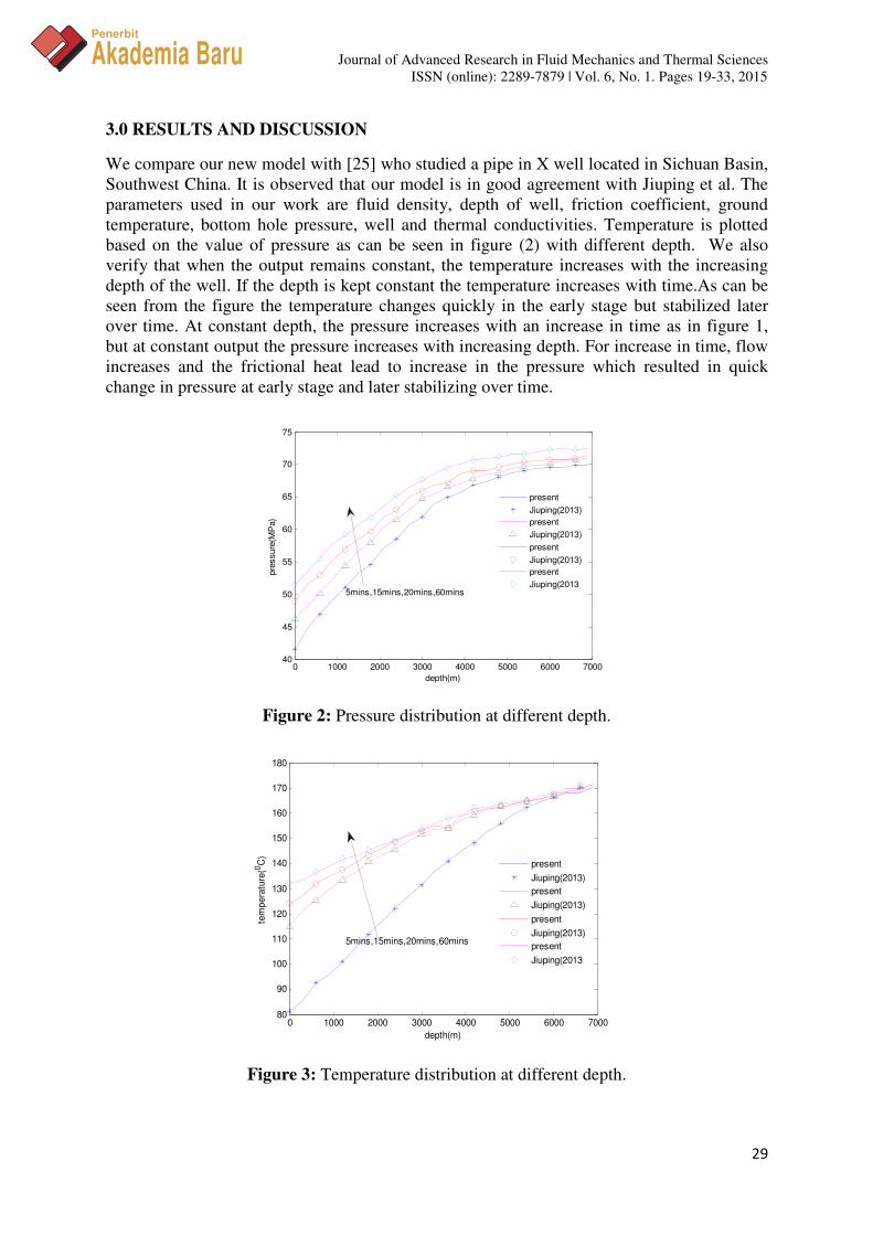
3.0 RESULTS AND DISCUSSION

We compare our new model with [25] who studied a pipe in X well located in Sichuan Basin,

Southwest China. It is observed that our model is in good agreement with Jiuping et al. The

parameters used in our work are fluid density, depth of well, friction coefficient, ground

temperature, bottom hole pressure, well and thermal conductivities. Temperature is plotted

based on the value of pressure as can be seen in figure (2) with different depth. We also

verify that when the output remains constant, the temperature increases with the increasing

depth of the well. If the depth is kept constant the temperature increases with time.As can be

seen from the figure the temperature changes quickly in the early stage but stabilized later

over time. At constant depth, the pressure increases with an increase in time as in figure 1,

but at constant output the pressure increases with increasing depth. For increase in time, flow

increases and the frictional heat lead to increase in the pressure which resulted in quick

change in pressure at early stage and later stabilizing over time.

Figure 2: Pressure distribution at different depth.

Figure 3: Temperature distribution at different depth.

0 1000 2000 3000 4000 5000 6000 700040

45

50

55

60

65

70

75

depth(m)

pre

ssure

(MP

a)

present

Jiuping(2013)

present

Jiuping(2013)

present

Jiuping(2013)

present

Jiuping(20135mins,15mins,20mins,60mins

0 1000 2000 3000 4000 5000 6000 700080

90

100

110

120

130

140

150

160

170

180

depth(m)

tem

pera

ture

(0C

)

present

Jiuping(2013)

present

Jiuping(2013)

present

Jiuping(2013)

present

Jiuping(2013

5mins,15mins,20mins,60mins



30

Penerbit

Akademia Baru

Due to the joule thermal effect, the temperature of the hot fluid at the bottom is not equal to

the temperature of the formation at the same depth. After the gas rises up along the tubing,

the temperature difference with the surrounding increases as the formation temperature

reduces. As shown in figure 3 the temperature rises as time increases. We consider different

thermal conductivities of the earth at different times and the result shows that it has an effect

on the distribution of temperature between the formation and the tubing as shown in figure 4.

Figure 4: Temperature changes in the surrounding.

Figure 5: Different values of thermal conductivities depth at different time at different time.

4.0 CONCLUSSION

Previous predictions have shown that the ability to predict flowing fluid temperature and

pressure has become necessary in several design problems that arise in gas production. In our

work, we present a system of partial differential equations based on Newton’s second law of

motion. The model is based on mass, momentum and the interrelation of pressure,

temperature, gas velocity and density of flowing gas in producing gas well. The solution to

the steady state became our boundary condition as required by flow propagation.We solve

0 1000 2000 3000 4000 5000 6000 70000

0.5

1

1.5

2

2.5

3

3.5te

mp

era

ture

depth

2unit

5unit

15unit

20unit

60unit

0 0.5 1 1.5 2 2.5 3 3.5 40

0.5

1

1.5

2

2.5

time

Dim

en

sio

nle

ss

te

mp

atu

re

ke=2.8

ke=3.2

ke=4.4

ke=5.3

ke=5.5

Final time of 4



31

Penerbit

Akademia Baru

our model using Finite Scheme ethod (FSM). The result is in good agreement with the work

of Wu et al. [23].

ACKNOWLEDGEMENT

Financial support provided by VOT 01G31, Research University Scheme, Universiti

Teknologi Malaysia is gratefully acknowledged.

REFERENCES

[1] B. E. Larock, R.W. Jeppson, G.Z. Watters, Calculation of unsteady gas flow through

porous media, Petroleum Geology and Oil Field Development, 1953.

[2] H. Daneshyar, One Dimensional Compressible Flow, Oxford New York Toronto

Sydney Paris Franfurt: Pergamon Press, 1976.

[3] H. Bin, Characterizing gas-lift Instabilities, Norwegian University of Science and

Technology, Trondheim, Norway, 2004.

[4] C.V. Kirkpatrick, Advances in gas-lift technology, Drill, Prodution, Practical, Journal

of Chemical Engineering Science 59 (1959) 24-60.

[5] H.J. Ramey, Wellbore Heat transmission, Journal of Petroleum Technology and

Science 225 (1962) 427-435.

[6] Ramey and Hasan, How to calculate Heat Transmission in Hot fluid injection, Journal

of Petroleum Engineering (1966).

[7] R. Sagar, D.R. Doty, Z. Schmldt, Predicting Temperature Profiles in a Flowing Well,

SPE Production Engineering 6 (1991) 441-448.

[8] A. Scatter, Heat losses during flow of steam down a wellbore, Journal of Petroleum

Technology (1965) 845-851.

[9] D. M. Coulter, M. F. Bardon, Revised Equation Improve Flowing Gas Temperature

Prediction Oil Gas, Journal of Petroleum Engineering 9 (1979) 107-115.

[10] J. Xu, Z. Wu, S. Wang, B. Qi, K. Chen, X. Li, X. Zhao, Prediction of Temperature,

Pressure, Density,Velocity Distribution in H-T-H-P Gas Wells, The Canadian Journal

of Chemical Engineering (2012).

[11] K. L. Young, Effect of assumption used to calculate bottomhole pressure in gas wells,

Journal of Petroleum Technology 19 (1967) 94-103.

[12] R. G. Agarwal, An investigation of wellbore storage and skin effect in unsteady liquid

flow, analytical treatment, Journal Society of Petroleum Engineering 10 (1969) 279-

290.

[13] A. Babatundo, Calculation of bottom hole pressure in a single phase gas wells from

wellhead measurement, Annual Technical Report of SPE, 1975.



32

Penerbit

Akademia Baru

[14] Osadacz, Simulation of Transient Gas Flow in Networks, International Journal

Numerical Methamatics Fluids 4 (1984) 13-24.

[15] X. Zhao, J. Xu, Numerical Simulation of Temperature and Pressure Distribution in

Producing Gas Well, World Journal of Modelling and Simulation 4 (2008) 294-303.

[16] A.R. Hasan, C.S. Kabir, Heat transfer during two-phase flow in wellbores: Part 1—

Formation temperature SPE Paper No. 22866, SPE Annual Technical Conference and

Exhibition, 1991.

[17] A.R. Hasan, C.S. Kabir, Wellbore Heat Transfer Modelling and Applications, SPE

Journal 86 (2012) 127-136.

[18] A.R. Hasan, C.S. Kabir, A Mechanistic model for computing fluid temperature profile

in gas lift wells, SPE Journal 11 (1996) 1-7.

[19] L. Yongming, Z. Jinzhou, G. Yang, Y. Fengsheng, J. Youshi, Unsteady Flow Model

for Fractured Gas Reservoirs, International Conference on Computational and

Information Sciences (2010) 978 4270.

[20] H. Bin, Characterizing gas-lift instabilities, NTNU, Department of Petroleum

Engineering and Applied Geophysics Norwegian University of Science and

Technology Trondheim, Norway, 2004.

[21] O.C. Candia, A. Mario, Prediction of pressure, temperature, and velocity distribution

of two phase flow in oil wells, Journal of Society of Petroleum Engineering 46 (2005)

195-208.

[22] B. M. Hameed, F. L. Rasheed, A. K. Abba, Analytical and Numerical Investigation of

Transient Gas Blow down, Modern Applied Science 5 (2011) 64-72.

[23] J. Xu, M. Luo, J. Hu, S. Wang, B. Qi, Z. Qiao, A direct Eulurian GRP Schemes for

the Prediction of Gas liquid two phase in HPHT transient gas wells, Journal of

Abstruct and Applied Analysis 2013 (2013) 1-7.

[24] Tong et al., Transient Simulation of Wellbore Pressure and Temperature during Gas

Well testing (JERT), 2014.

[25] O. D. Orodu, C.T. Ako, F. A. Makinde, M.O Owarume, Well deliverability Prediction

of Gas flow in a Gas condensate reservoirs. Modeling near two phase in one

dimension, Brazilian Journal of Petroleum and gas, 6 (2012) 159-169.

[26] M. Li, L. Sun, S. Li, New View on Continuous-removal Liquids from Gas Wells,

Proceedings of the 2001 Proceedings of the Permian Basin Oil and Gas Recovery

Conference of SPE Midland, 2013.

[27] A. Scatter, Heat losses during flow of steam down a wellbore, Journal of Petroleum

Technology 234 (1965) 845-851.

[28] Z. Fonzong, Research on heat transfer in Geothermal wellbore and surrounding.

Master Thesis, Planen bauen umwelt der technischen universität, Germany 2013.

[29] M. Finley, BP Statistical Review of World Energy, Energy Reviewed Report, 2013.



33

Penerbit

Akademia Baru

[30] R.M. Cullender, R.V. Smith, Practical solution of flow equations for wells and pipes

with large gradient, Trans AIME 207 (1956) 281-287.

[31] B. Bai, X. C. Li, M. Z. Liu, L. Shi, Q. Li et al., A fast finite difference method for

determination of wellhead injection pressure, Journal of Central South University 19

(2012) 3266-3272.

[32] Brills, Murhejee, Multiphase flow, Journal Petroleum Technology (1999).

modelling unsteady flow of gas and heat transfer in...

Documents