Plant and Soil 239: 19–38, 2002.© 2002 Kluwer Academic Publishers. Printed in the Netherlands.

19

Modelling root growth

Modelling the interactions between water and nutrient uptake and rootgrowth

Vanessa M. Dunbabin1,2,4,∗, Art J. Diggle2,3, Zdenko Rengel1,2 & Robert van Hugten2

1Department of Soil Science and Plant Nutrition, The University of Western Australia, 35 Stirling Highway, Craw-ley WA 6009, Australia, 2Centre for Legumes in Mediterranean Agriculture, The University of Western Australia, 35Stirling Highway, Crawley WA 6009, Australia, and 3Western Australian Department of Agriculture, Baron-HayCourt, South Perth WA 6151, Australia, 4Corresponding author∗

Key words: computer modelling, N2 fixation, nitrate uptake, relative inflow, resource partitioning, root plasticity

Abstract

A model of three-dimensional root growth has been developed to simulate the interactions between root systems,water and nitrate in the rooting environment. This interactive behaviour was achieved by using an external-supply/internal-demand regulation system for the allocation of endogenous plant resources. Data from potexperiments on lupins heterogeneously supplied with nitrate were used to test and parameterise the model forfuture simulation work. The model reproduced the experimental results well (R2 = 0.98), simulating both theroot proliferation and enhanced nitrate uptake responses of the lupins to differential nitrate supply. These resultssupport the use of the supply/demand regulation system for modelling nitrate uptake by lupins. Further simulationwork investigated the local uptake response of lupins when nitrate was supplied to a decreasing fraction of theroot system. The model predicted that the nitrate uptake activity of lupin roots will increase as the fraction of rootsystem with access to nitrate decreases, but is limited to an increase of around twice that of a uniformly suppliedcontrol. This work is the first example of a modelled root system responding plastically to external nutrient supply.This model will have a broad range of applications in the study of the interactions between root systems and theirspatially and temporally heterogeneous environment.

Introduction

Ever increasing computing power has allowed the de-velopment of models that simulate root growth inthree-dimensional space (Diggle, 1988a; Lynch et al.,1997; Pagès et al., 1989). While considerable workhas gone into studying the response of root systems totheir local environment (Bingham et al., 1997; Drew,1975; Drew and Saker, 1975, 1978; Drew et al.,1973; Fitter and Stickland, 1991; Fitter et al., 1988;Gersani and Sachs, 1992; Robinson, 1994, 1996),much remains to be determined about the mechan-isms behind these root responses. This has limitedthe ability of three-dimensional root growth models to

∗ FAX: +61 3 6253 5558;E-mail: vdunbabi@agric.uwa.edu.au

include interactions between roots systems and theirenvironment.

It has been recognised for some time that bothroot and shoot growth are a function of resource parti-tioning within the plant. Early one-dimensional plantgrowth models included the partitioning of resources,typically carbon and nitrogen, and their influence onthe growth rate of the root and shoot systems (Bald-win, 1976; Raper et al., 1978; Thornley, 1972). Nye etal. (1975) produced a model of root and shoot growthdependent upon the supply of phosphorus to the rootsystem. Lim et al. (1990) modelled responses of non-nodulated soya bean plants to nitrate supply using acarbon and nitrogen partitioning scheme developedfrom the earlier model of Thornley (1972).

Despite the existence of these good early models,the incorporation of resource partitioning strategies

20

into three-dimensional root growth models is only nowbeginning to occur. Somma et al. (1998) were amongthe first to incorporate the nutrient status of the entireplant as a factor in the three-dimensional modelling ofroot growth. In their model, root elongation is affectedby temperature, soil strength and nutrient concentra-tion when these properties fall outside an optimumrange, and the resultant elongation is scaled accordingto the amount of biomass allocated to the root system.Thaler and Pagès (1998) have also made root growtha function of assimilate availability in their model, butthe growth of individual root tips is not affected bybelow-ground resources.

The objective of this paper is to describe a modelof three-dimensional root growth that takes a differ-ent approach to other recent models. It uses the plantdemand for individual resources and the ability ofvarious components of the plant to supply individualresources to drive the allocation of endogenous assim-ilates and subsequent local root growth, architecturaldevelopment and nutrient uptake rates. The model isbased on the framework of a three-dimensional rootarchitecture model (Diggle, 1988a) which has beenextended to include nutrient and water transport anduptake.

The model can effectively simulate the growth oflegumes. Experimental data for the nitrate uptake androot growth response of two lupin species, Lupinusangustifolius and L. pilosus, to heterogeneously sup-plied nitrate in solution (Dunbabin et al., 2001a,b), areused to calibrate the model for future lupin modellingwork. The internal relationships used by the model toreproduce the experimental data are presented.

The model

Model equations and symbol definitions can be foundin Appendix 1.

Model structure

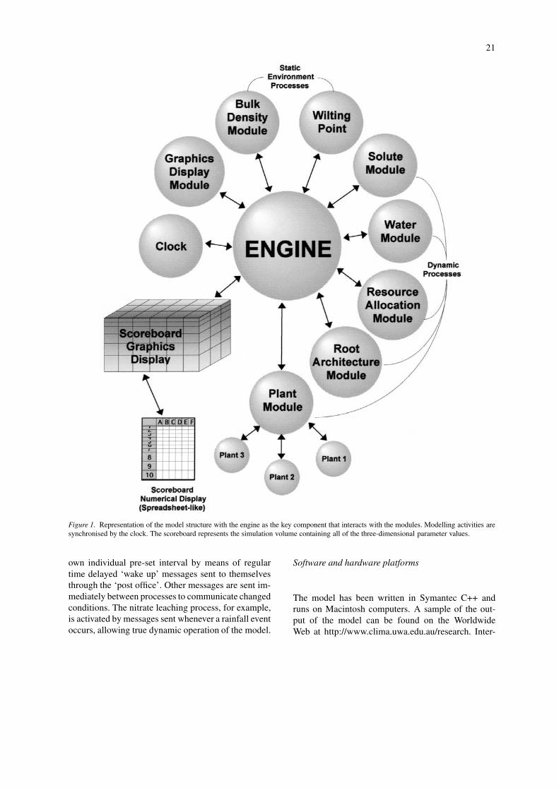
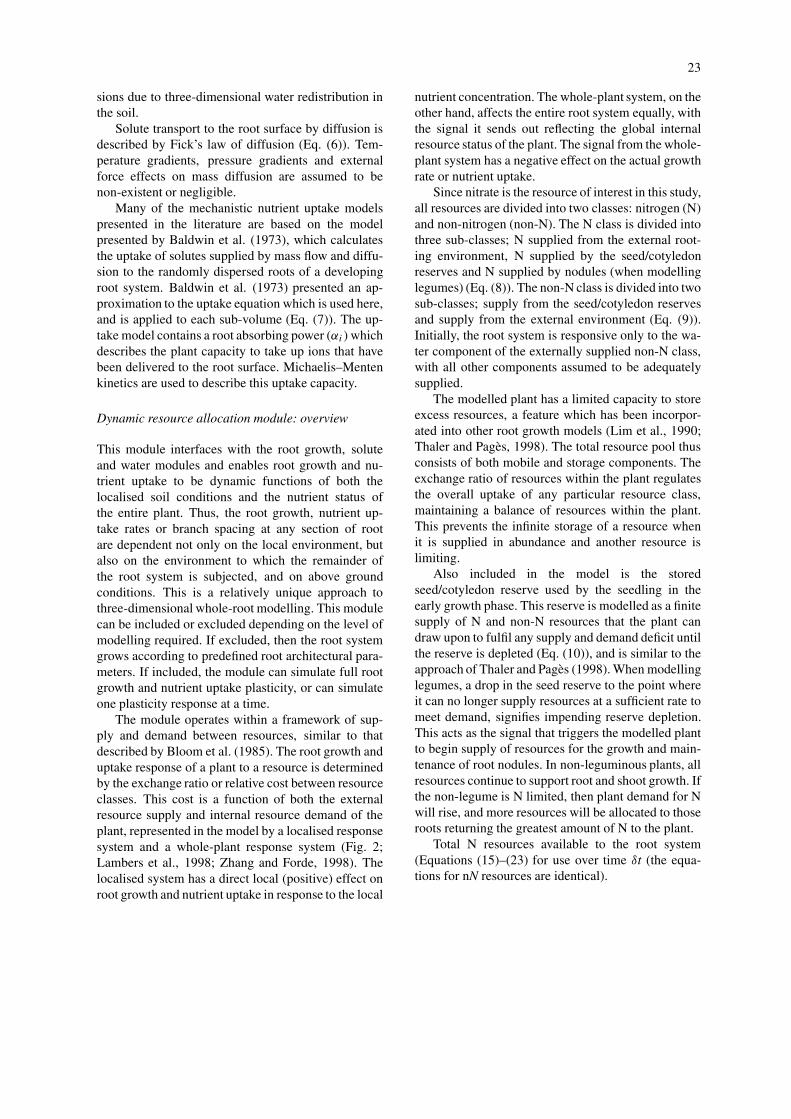
The model has been developed as an object-oriented,modular program for simulating plant and soil pro-cesses. The four key components of the model arethe engine, the scoreboard structure, the ‘plug-in’modules, and the asynchronous clock (Fig. 1).

(1) The engine is the central control mechanismand inter-module communicator. It sends messages toall of the modules and acts upon the responses. Allof the modules communicate with each other via theengine.

(2) The simulation volume is represented by aseries of scoreboards, which are three-dimensionalrectangular volumes, divided into layers in each dir-ection that are not required to be of regular or equalsize. The boxes or sub-volumes created by the in-tersection of the layers store the local characteristicsrequired by, or created by, each of the process mod-ules (e.g. water content, nitrate concentration, rootlength). This allows the soil volume to be modelledas both a heterogeneous and dynamic entity. The char-acteristics of each sub-volume are updated each timea process affects the volume, such as when water andnitrate leach through a volume, or nitrate is taken up.Each process can store information generated by thatprocess and retrieve information from the scoreboardprovided by other processes at any point in time. Theinformation in scoreboards can be state variables orit can be summary information about state variables.All communication of information between processesis done via the scoreboards. The scoreboard is also auser interface, providing information on any numberof characteristics in any sub-volume within the totalsimulation volume at any point during the simulation.This information can be exported into spreadsheetpackages for further analysis or graphical represent-ation. The user can feed information back into someof the modules by editing values in the scoreboard.The scoreboard system is very flexible as it allowsmodelling on both a field level and the micro-processlevel.

(3) The ‘plug-in’ modules (e.g., nitrate module,plant module, Fig. 1) interact with the engine via mes-sages. The majority are dynamic process modules,which affect an action in the simulation volume (e.g.,growth, leaching, uptake). They require informationfrom other modules as stored in the scoreboard viathe engine, and they pass information into the score-board for use by other modules or the user. Thereare also static modules which are generally preset,time-independent attributes.

(4) The asynchronous clock allows each of themodules to operate according to significant events ofrelevance to that process, rather than in rigid timesteps. This allows each of the modules to operateat different time scales and react to events, such asrainfall, that occur at non-rigid points in time. Thisasynchronous operation is managed by the ‘post of-fice’ which coordinates the delivery of messages sentbetween the process modules via the engine. The mes-sages all have a recipient process or processes, and atime for delivery. Some processes are activated at their

21

Figure 1. Representation of the model structure with the engine as the key component that interacts with the modules. Modelling activities aresynchronised by the clock. The scoreboard represents the simulation volume containing all of the three-dimensional parameter values.

own individual pre-set interval by means of regulartime delayed ‘wake up’ messages sent to themselvesthrough the ‘post office’. Other messages are sent im-mediately between processes to communicate changedconditions. The nitrate leaching process, for example,is activated by messages sent whenever a rainfall eventoccurs, allowing true dynamic operation of the model.

Software and hardware platforms

The model has been written in Symantec C++ andruns on Macintosh computers. A sample of the out-put of the model can be found on the WorldwideWeb at http://www.clima.uwa.edu.au/research. Inter-

22

ested parties can contact the authors for a copy of acompiled version of the model.

The process modules

A number of process modules have been written (inC++) to account for factors such as: ammonium and itstransformations, extractable aluminium, phosphorusand pH (unpublished); temperature effects on rootgrowth and development and root growth resistance(Diggle, 1988b); root architectural development, dy-namic resource allocation, solute and water flows (seebelow). Many more modules could be incorporateddepending upon the type of modelling required. Eachof the modules can be included or excluded as requiredfor different levels of modelling. Some of the modulesare described here.

Three-dimensional root growth and structure module

The basic growth and structural development of theroot system is carried out by Diggle’s (1988a) three-dimensional root architectural model, ROOTMAP.Full details of the parameters, methodology and func-tion of the architectural model can be found in Diggle(1988a–c). The model applies a set of growth rules toa series of root types or classes, with each root typehaving its own characteristic set of growth parameters(Diggle, 1988a). Root elongation rate (Gi), branchingdensity (Bi), and branching lag time (Tb) are the maingrowth parameters used in the model (Diggle, 1988a).The radial position of branch growth around an axis isdetermined at random (Diggle, 1988b). The directionof root growth is determined stochastically from a de-flection index (tendency to deflect from the previousgrowth direction) and a geotropism index (tendencyfor a root to grow preferentially downward) (Diggle,1988b). The stochastic elements of the model allowroot systems to bend and deflect in a similar way tothat observed in the field, without requiring know-ledge of the complex phenomena which govern rootdeflections (Pagès, 1999).

All root architectural parameters can be pre-allocated, restricting simulated root systems to growin a pre-defined fashion. In addition, a feedback-basedresponse module can be used to dynamically allocatethe main growth parameters. This allows the plant toadjust its growth through both time and space based onresource availability (see dynamic resource allocationmodule below).

Water module

This module incorporates the drainage, redistribution,evaporation and uptake of water from the rooting en-vironment. Drainage is simulated using a capacitymodel. This method of modelling water movementdefines changes rather than rates of change in watercontent (Addiscott and Wagenet, 1985) and is idealfor applications with fast draining sandy soils (Roseet al., 1982a). The model is not expected to make ac-curate predictions for highly structured clays, or otherheavier soils that are highly heterogeneous in struc-ture (Addiscott, 1996). The format of the model does,however, allow modules that are tailored to these soilconditions to be easily incorporated. Capacity mod-els are used in many simulation models (see summaryby de Willigen, 1991; Probert et al., 1998), and arechosen because of their ease of implementation andthe ability to measure the relevant soil water capacitiesand avoid the spatial variability problems associatedwith the inputs required for rate models (Addiscott andWagenet, 1985).

The redistribution of water in three-dimensionswithin the profile is based on Darcy’s Law (Eq. (1))(Richards, 1931). The water uptake routine is basedon the standard sink term (Sw) used in many models ofwater flow and uptake by plant roots (Eq. (2)) (Feddeset al., 1976; Habib and Lafolie, 1991). This uptakeroutine uses a weighting function (αw) to describe theplant’s ability to extract water over a range of soil wa-ter potentials. A sigmoidal curve is used to describethe weighting function over the soil water potentialrange from drained upper limit to lower extractionlimit (Eq. (3)). The same weighting function is alsoused to calculate the evaporation of water from thesoil surface (Ew) based upon the maximum potentialevaporation rate (Emax) (Eq. (4)) and a dynamic factorthat accounts for plant cover (p(t)).

Solute module

The solute module incorporates leaching, mass flow,diffusion and uptake. There are a variety of approachesto modelling solute leaching in field soils. The modelchosen for this work (Rose et al., 1982a,b) is an ap-proximate solution to the convection–dispersion equa-tion. It is implemented in the same manner as Diggle(1990), where small ‘packets’ of nitrate (pseudo ions)represent the spread of nitrate ions through the profile(Eq. (5)). This method is also used to calculate themass flow or redistribution of nitrate in three dimen-

23

sions due to three-dimensional water redistribution inthe soil.

Solute transport to the root surface by diffusion isdescribed by Fick’s law of diffusion (Eq. (6)). Tem-perature gradients, pressure gradients and externalforce effects on mass diffusion are assumed to benon-existent or negligible.

Many of the mechanistic nutrient uptake modelspresented in the literature are based on the modelpresented by Baldwin et al. (1973), which calculatesthe uptake of solutes supplied by mass flow and diffu-sion to the randomly dispersed roots of a developingroot system. Baldwin et al. (1973) presented an ap-proximation to the uptake equation which is used here,and is applied to each sub-volume (Eq. (7)). The up-take model contains a root absorbing power (αi ) whichdescribes the plant capacity to take up ions that havebeen delivered to the root surface. Michaelis–Mentenkinetics are used to describe this uptake capacity.

Dynamic resource allocation module: overview

This module interfaces with the root growth, soluteand water modules and enables root growth and nu-trient uptake to be dynamic functions of both thelocalised soil conditions and the nutrient status ofthe entire plant. Thus, the root growth, nutrient up-take rates or branch spacing at any section of rootare dependent not only on the local environment, butalso on the environment to which the remainder ofthe root system is subjected, and on above groundconditions. This is a relatively unique approach tothree-dimensional whole-root modelling. This modulecan be included or excluded depending on the level ofmodelling required. If excluded, then the root systemgrows according to predefined root architectural para-meters. If included, the module can simulate full rootgrowth and nutrient uptake plasticity, or can simulateone plasticity response at a time.

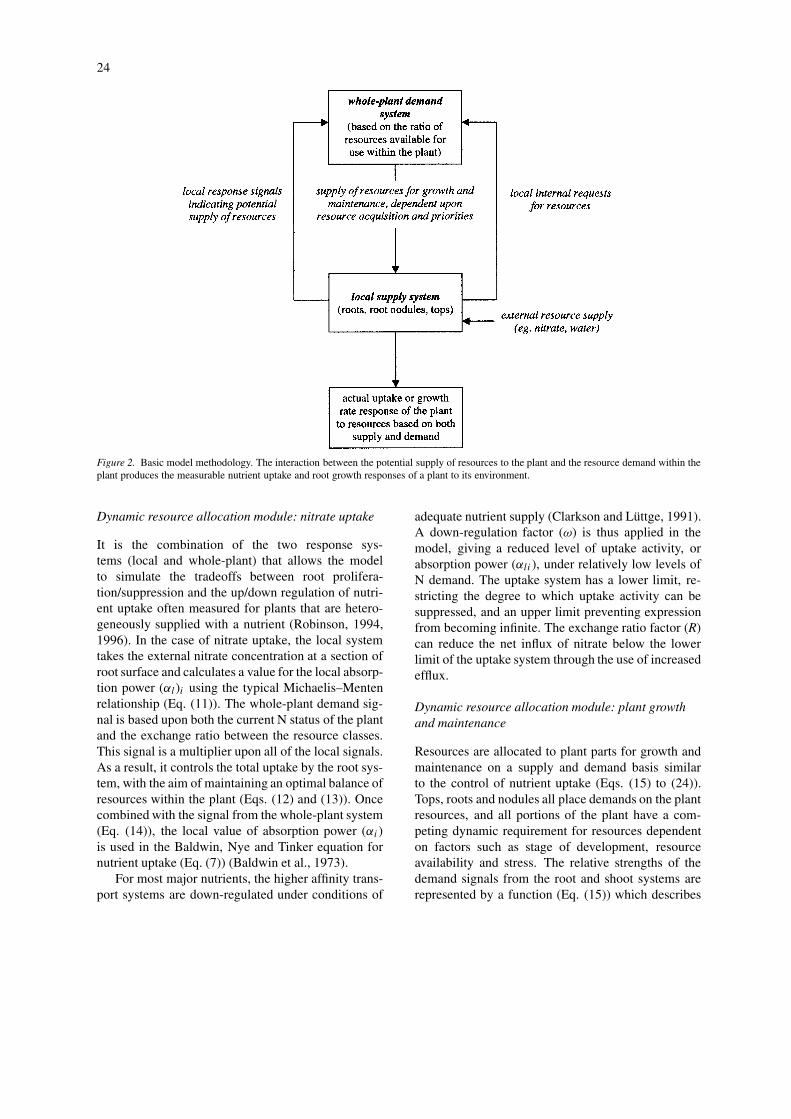
The module operates within a framework of sup-ply and demand between resources, similar to thatdescribed by Bloom et al. (1985). The root growth anduptake response of a plant to a resource is determinedby the exchange ratio or relative cost between resourceclasses. This cost is a function of both the externalresource supply and internal resource demand of theplant, represented in the model by a localised responsesystem and a whole-plant response system (Fig. 2;Lambers et al., 1998; Zhang and Forde, 1998). Thelocalised system has a direct local (positive) effect onroot growth and nutrient uptake in response to the local

nutrient concentration. The whole-plant system, on theother hand, affects the entire root system equally, withthe signal it sends out reflecting the global internalresource status of the plant. The signal from the whole-plant system has a negative effect on the actual growthrate or nutrient uptake.

Since nitrate is the resource of interest in this study,all resources are divided into two classes: nitrogen (N)and non-nitrogen (non-N). The N class is divided intothree sub-classes; N supplied from the external root-ing environment, N supplied by the seed/cotyledonreserves and N supplied by nodules (when modellinglegumes) (Eq. (8)). The non-N class is divided into twosub-classes; supply from the seed/cotyledon reservesand supply from the external environment (Eq. (9)).Initially, the root system is responsive only to the wa-ter component of the externally supplied non-N class,with all other components assumed to be adequatelysupplied.

The modelled plant has a limited capacity to storeexcess resources, a feature which has been incorpor-ated into other root growth models (Lim et al., 1990;Thaler and Pagès, 1998). The total resource pool thusconsists of both mobile and storage components. Theexchange ratio of resources within the plant regulatesthe overall uptake of any particular resource class,maintaining a balance of resources within the plant.This prevents the infinite storage of a resource whenit is supplied in abundance and another resource islimiting.

Also included in the model is the storedseed/cotyledon reserve used by the seedling in theearly growth phase. This reserve is modelled as a finitesupply of N and non-N resources that the plant candraw upon to fulfil any supply and demand deficit untilthe reserve is depleted (Eq. (10)), and is similar to theapproach of Thaler and Pagès (1998). When modellinglegumes, a drop in the seed reserve to the point whereit can no longer supply resources at a sufficient rate tomeet demand, signifies impending reserve depletion.This acts as the signal that triggers the modelled plantto begin supply of resources for the growth and main-tenance of root nodules. In non-leguminous plants, allresources continue to support root and shoot growth. Ifthe non-legume is N limited, then plant demand for Nwill rise, and more resources will be allocated to thoseroots returning the greatest amount of N to the plant.

Total N resources available to the root system(Equations (15)–(23) for use over time δt (the equa-tions for nN resources are identical).

24

Figure 2. Basic model methodology. The interaction between the potential supply of resources to the plant and the resource demand within theplant produces the measurable nutrient uptake and root growth responses of a plant to its environment.

Dynamic resource allocation module: nitrate uptake

It is the combination of the two response sys-tems (local and whole-plant) that allows the modelto simulate the tradeoffs between root prolifera-tion/suppression and the up/down regulation of nutri-ent uptake often measured for plants that are hetero-geneously supplied with a nutrient (Robinson, 1994,1996). In the case of nitrate uptake, the local systemtakes the external nitrate concentration at a section ofroot surface and calculates a value for the local absorp-tion power (αl)i using the typical Michaelis–Mentenrelationship (Eq. (11)). The whole-plant demand sig-nal is based upon both the current N status of the plantand the exchange ratio between the resource classes.This signal is a multiplier upon all of the local signals.As a result, it controls the total uptake by the root sys-tem, with the aim of maintaining an optimal balance ofresources within the plant (Eqs. (12) and (13)). Oncecombined with the signal from the whole-plant system(Eq. (14)), the local value of absorption power (αi)is used in the Baldwin, Nye and Tinker equation fornutrient uptake (Eq. (7)) (Baldwin et al., 1973).

For most major nutrients, the higher affinity trans-port systems are down-regulated under conditions of

adequate nutrient supply (Clarkson and Lüttge, 1991).A down-regulation factor (ω) is thus applied in themodel, giving a reduced level of uptake activity, orabsorption power (αli ), under relatively low levels ofN demand. The uptake system has a lower limit, re-stricting the degree to which uptake activity can besuppressed, and an upper limit preventing expressionfrom becoming infinite. The exchange ratio factor (R)can reduce the net influx of nitrate below the lowerlimit of the uptake system through the use of increasedefflux.

Dynamic resource allocation module: plant growthand maintenance

Resources are allocated to plant parts for growth andmaintenance on a supply and demand basis similarto the control of nutrient uptake (Eqs. (15) to (24)).Tops, roots and nodules all place demands on the plantresources, and all portions of the plant have a com-peting dynamic requirement for resources dependenton factors such as stage of development, resourceavailability and stress. The relative strengths of thedemand signals from the root and shoot systems arerepresented by a function (Eq. (15)) which describes

25

the root system as the primary resource sink duringthe early developmental phase, with a gradual shift inproportional demand towards the tops as they developand become a large resource sink, particularly duringthe reproductive phases of growth. The various rootclasses are given different resource priorities (µg) (Eq.(20)). The tap root, for example, is given a higher non-N priority (µgnN) than laterals, making its growth lessresponsive to nitrate supply, fulfilling the requirementfor the exploration of non-N resources such as deepstored water (Hamblin and Hamblin, 1985; Hamblinand Tennant, 1987; White, 1990).

Dynamic resource allocation module: N2 fixation

When modelling lupins (the initial target species), it isassumed that the reliance on fixation varies in responseto the external nitrate supply, as supported by experi-ments showing a reduction in the level of N2 fixation inlupins in response to increased edaphic nitrate supply(Cowie et al., 1990a,b). Resources are allocated to theroot nodules based on the current level of N fixation,and the demand for an increase (or decrease) in fix-ation created by a deficit (or excess) in N supply byuptake from the rooting environment (Eqs. (23) and(22)). When plant growth is N limited, resources aresupplied in excess of that required for maintenance ofthe nodules leading to an increase in the number ofnodules, and vice versa (Eqs. (26) and (27)). Undertypical conditions, the simulated percentage of totalN supplied by fixation falls within the typical fixationrange for lupins of 56–89% (Anderson et al., 1998a,b;Evans et al., 1987).

Validation of the dynamic resource allocationmodule

Method

To test and parameterise the model for future rootmodelling work on lupins, the model was used tosimulate two split-root nutrient solution experiments.These experiments were designed to study the rootgrowth (Dunbabin et al., 2001a) and nitrate uptake(Dunbabin et al., 2001b) response of two lupin spe-cies, Lupinus pilosus Murr. and L. angustifolius L.,to the spatially heterogeneous supply of nitrate. Thesetwo species were selected because they represent theextremes of the root morphology types across the lupingermplasm, with L. angustifolius having a dominanttap root and primary lateral system, and L. pilosus a

less dominant tap root and well developed lateral sys-tem with primary, secondary and tertiary laterals allpresent (Clements et al., 1993). The full experimentaldetails are described in Dunbabin et al. (2001 a,b), andare explained again below in brief.

Nitrate uptake experiment

At 8 weeks of age nodulated plants of both species(L. pilosus and L. angustifolius) were placed in ver-tically split chambers in a controlled growth roomenvironment. Inspection of plant nodules revealed thatall plants were fixing nitrogen at this age (Dunbabinet al., 2001b). Aerated nutrient solution was suppliedto the root system at three nitrate rates 250, 750 and1500 µM as a uniform supply to the upper and lowerroot system or a split high/low or low/high supply(e.g., 750/250, 250/750, 1500/250 or 250/1500 µMNO3

−, the treatments are always described by theirnitrate concentrations in the format: upper root sys-tem/lower root system). All plants were grown in auniform nutrient solution with a nitrate concentrationof 250 µm before application of treatments. The totaltreatment period was 12 h (the entire light phase) andthe solution was sampled at half-hourly intervals todetermine the depletion of nitrate from solution andcalculate the nitrate uptake rate. Nitrate was not fullydepleted from solution after 12 h. Depletion data wereused to calculate the net inflow as a function of thenitrate concentration in solution. A curve followingthe Michaelis–Menten equation was then fitted to themeasured data by estimating the parameters by theleast squares method. Total plant transpiration wasestimated by calculating the water balance betweeninitial water volume, volume removed in sampling,and final solution volume. A transpiration rate wasthen linearly interpolated over the 12 h. This was usedas an estimate of the maximum potential transpirationrate under conditions of no soil resistance to watermovement.

L. angustifolius was found to have a plastic netinflux response (elevated uptake kinetics) to localisednitrate supply, while L. pilosus did not (Dunbabin etal., 2001b). Thus, for L. angustifolius in a non-uniformsupply treatment, the nitrate uptake rate in the high ni-trate zone was higher than if the root system had beenuniformly supplied with that high nitrate rate. Cor-respondingly, the uptake rate in the low nitrate zonewas lower than if the root system had been uniformlysupplied with low nitrate (Dunbabin et al., 2001b).

26

For simulation of this experiment, a virtual plantwas set up in the same manner as the experimentalplant. Plants of both species were grown to 8 weeksof age at which time the treatments were imposed for12 h. A barrier was imposed in the model at the heightof the barrier in the experiment, to prevent exchangeof nutrient solution between the modelled upper andlower root system. Since there are no supply impedi-ments in nutrient solution, uptake for this simulationwas calculated purely on the basis of plant demandusing Michealis–Menten kinetics. The diffusion coef-ficient for nitrate in free solution (1.9×10−9 m2 s−1)was used to describe nitrate diffusion. The modelledtotal nitrate uptake over the 12 h was recorded, and theuptake rate linearly interpolated over these 12 h, forcomparison with the experimental data. Nitrate wasnot fully depleted from the modelled solution after12 h.

Root growth experiment

At 3 weeks of age, nodulated seedlings of both spe-cies (L. pilosus and L. angustifolius) were placed invertically split pots in a controlled growth room en-vironment. Aerated nutrient solution was supplied tothe root system at two nitrate rates, 250 or 750 µMas a uniform supply to the upper and lower root sys-tem or a split supply, e.g., 750/250 or 250/750 µMNO3

−. All plants were grown in a uniform nutrientsolution with a nitrate concentration of 250 µM be-fore application of treatments. Treatment period was9 days, with root length (separated into root classes,e.g., tap root, and various orders of laterals of the up-per and lower root system) measured before and aftertreatment application. The growth of the various rootclasses over the 9 days was compared. Root growthwas found to be correlative in both species (increasein root growth in a high nitrate patch accompaniedby a decrease in growth in the low nitrate patch giv-ing approximately the same total growth, (Gersani andSachs, 1992; Robinson, 1996), with L. pilosus havinga larger growth response to a high nitrate zone than L.angustifolius, particularly in the growth of the secondorder laterals (Dunbabin et al., 2001a).

Again, the simulation was designed to mimic theexperiment. The simulation was run until the plantwas 3 weeks of age, at which stage the split or uni-form treatments were imposed for 9 days. The set-upof the model and all parameters were identical tothose used for the nitrate uptake simulation. Solutioncould not pass between the upper and lower root sys-

tem in the simulated volume. The total modelled rootlength for each branch order was recorded at the startof the treatment period and again at the end of thetreatment period, with the growth rates linearly inter-polated between the two times, for comparison withthe experimental data.

Model parameters

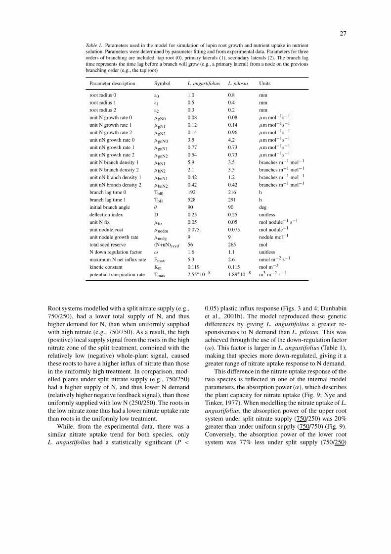
Model parameters such as the potential transpirationrate, Michaelis–Menten constants, root radii, branchspacing, and seed reserve ratio (related to the seedweight ratio), were derived directly from the twogrowth room experiments (Table 1). The remainingparameters were calibrated by comparison to the ex-perimental data. The unit growth rates, for example,were adjusted until the observed growth rates weresimulated. The down regulation factor (ω) was in-creased until the observed level of uptake plasticitywas simulated. This is essentially a process of measur-ing an otherwise unquantifiable plant trait, such as thegenetic capacity for nutrient uptake plasticity.

Model output

Subsequent to the calibration process, the model pre-dicted all experimental data well (R2 = 0.98, plot notshown) with most of the modelled data falling withinone standard error of the mean of the experimentaldata (Figs. 3–7). The model reproduced the nitrateuptake rate (Figs. 3 and 4) and root growth rate (Figs.5–7) characteristics of both species, under conditionsof uniform and heterogeneous nitrate supply. This sup-ports the general model hypothesis that the control ofplant root growth and nitrate uptake can be representedby a supply/demand regulation system that determinesresource allocation for root growth and nitrate uptake.An example of the diagrammatical output of the modelis given for the 1500/250 µM NO3

−-N treatment inthe nitrate uptake simulation (Fig. 8).

Nitrate uptake

The model simulated not only the increased uptakerate with increasing external nitrate concentration, butalso the plastic uptake response to heterogeneous ni-trate supply (Figs. 3 and 4). This was achieved throughthe interactions between the local supply system andthe whole-plant demand system (Fig. 2). These in-teractions can best be understood by comparing thebehaviour of modelled plants under split nitrate sup-ply to that under uniform high or low nitrate supply.

27

Table 1. Parameters used in the model for simulation of lupin root growth and nutrient uptake in nutrientsolution. Parameters were determined by parameter fitting and from experimental data. Parameters for threeorders of branching are included: tap root (0), primary laterals (1), secondary laterals (2). The branch lagtime represents the time lag before a branch will grow (e.g., a primary lateral) from a node on the previousbranching order (e.g., the tap root)

Parameter description Symbol L. angustifolius L. pilosus Units

root radius 0 a0 1.0 0.8 mm

root radius 1 a1 0.5 0.4 mm

root radius 2 a2 0.3 0.2 mm

unit N growth rate 0 µgN0 0.08 0.08 µm mol−1s−1

unit N growth rate 1 µgN1 0.12 0.14 µm mol−1s−1

unit N growth rate 2 µgN2 0.14 0.96 µm mol−1s−1

unit nN growth rate 0 µgnN0 3.5 4.2 µm mol−1s−1

unit nN growth rate 1 µgnN1 0.77 0.73 µm mol−1s−1

unit nN growth rate 2 µgnN2 0.54 0.73 µm mol−1s−1

unit N branch density 1 µbN1 5.9 3.5 branches m−1 mol−1

unit N branch density 2 µbN2 2.1 3.5 branches m−1 mol−1

unit nN branch density 1 µbnN1 0.42 1.2 branches m−1 mol−1

unit nN branch density 2 µbnN2 0.42 0.42 branches m−1 mol−1

branch lag time 0 Tbl0 192 216 h

branch lag time 1 Tbl1 528 291 h

initial branch angle θ 90 90 deg

deflection index D 0.25 0.25 unitless

unit N fix µfix 0.05 0.05 mol nodule−1 s−1

unit nodule cost µnodm 0.075 0.075 mol nodule−1

unit nodule growth rate µnodg 9 9 nodule mol−1

total seed reserve (N+nN)seed 56 265 mol

N down regulation factor ω 1.6 1.1 unitless

maximum N net influx rate Fmax 5.3 2.6 nmol m−2 s−1

kinetic constant Km 0.119 0.115 mol m−3

potential transpiration rate Tmax 2.55∗10−8 1.89∗10−8 m3 m−2 s−1

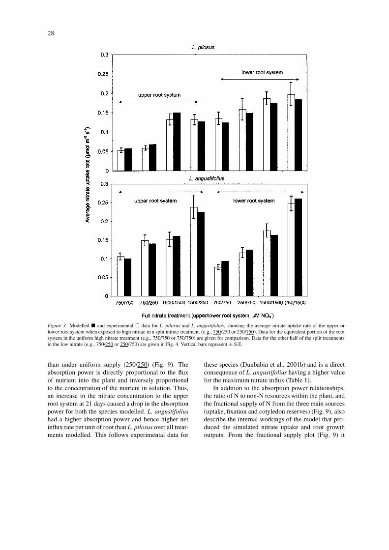
Root systems modelled with a split nitrate supply (e.g.,750/250), had a lower total supply of N, and thushigher demand for N, than when uniformly suppliedwith high nitrate (e.g., 750/750). As a result, the high(positive) local supply signal from the roots in the highnitrate zone of the split treatment, combined with therelatively low (negative) whole-plant signal, causedthese roots to have a higher influx of nitrate than thosein the uniformly high treatment. In comparison, mod-elled plants under split nitrate supply (e.g., 750/250)had a higher supply of N, and thus lower N demand(relatively higher negative feedback signal), than thoseuniformly supplied with low N (250/250). The roots inthe low nitrate zone thus had a lower nitrate uptake ratethan roots in the uniformly low treatment.

While, from the experimental data, there was asimilar nitrate uptake trend for both species, onlyL. angustifolius had a statistically significant (P <

0.05) plastic influx response (Figs. 3 and 4; Dunbabinet al., 2001b). The model reproduced these geneticdifferences by giving L. angustifolius a greater re-sponsiveness to N demand than L. pilosus. This wasachieved through the use of the down-regulation factor(ω). This factor is larger in L. angustifolius (Table 1),making that species more down-regulated, giving it agreater range of nitrate uptake response to N demand.

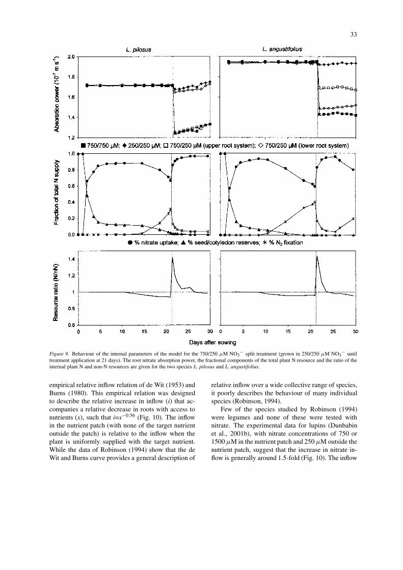
This difference in the nitrate uptake response of thetwo species is reflected in one of the internal modelparameters, the absorption power (α), which describesthe plant capacity for nitrate uptake (Fig. 9; Nye andTinker, 1977). When modelling the nitrate uptake of L.angustifolius, the absorption power of the upper rootsystem under split nitrate supply (750/250) was 20%greater than under uniform supply (750/750) (Fig. 9).Conversely, the absorption power of the lower rootsystem was 77% less under split supply (750/250)

28

Figure 3. Modelled � and experimental � data for L. pilosus and L. angustifolius, showing the average nitrate uptake rate of the upper orlower root system when exposed to high nitrate in a split nitrate treatment (e.g., 750/250 or 250/750). Data for the equivalent portion of the rootsystem in the uniform high nitrate treatment (e.g., 750/750 or 750/750) are given for comparison. Data for the other half of the split treatmentsin the low nitrate (e.g., 750/250 or 250/750) are given in Fig. 4. Vertical bars represent ± S.E.

than under uniform supply (250/250) (Fig. 9). Theabsorption power is directly proportional to the fluxof nutrient into the plant and inversely proportionalto the concentration of the nutrient in solution. Thus,an increase in the nitrate concentration to the upperroot system at 21 days caused a drop in the absorptionpower for both the species modelled. L. angustifoliushad a higher absorption power and hence higher netinflux rate per unit of root than L. pilosus over all treat-ments modelled. This follows experimental data for

these species (Dunbabin et al., 2001b) and is a directconsequence of L. angustifolius having a higher valuefor the maximum nitrate influx (Table 1).

In addition to the absorption power relationships,the ratio of N to non-N resources within the plant, andthe fractional supply of N from the three main sources(uptake, fixation and cotyledon reserves) (Fig. 9), alsodescribe the internal workings of the model that pro-duced the simulated nitrate uptake and root growthoutputs. From the fractional supply plot (Fig. 9) it

29

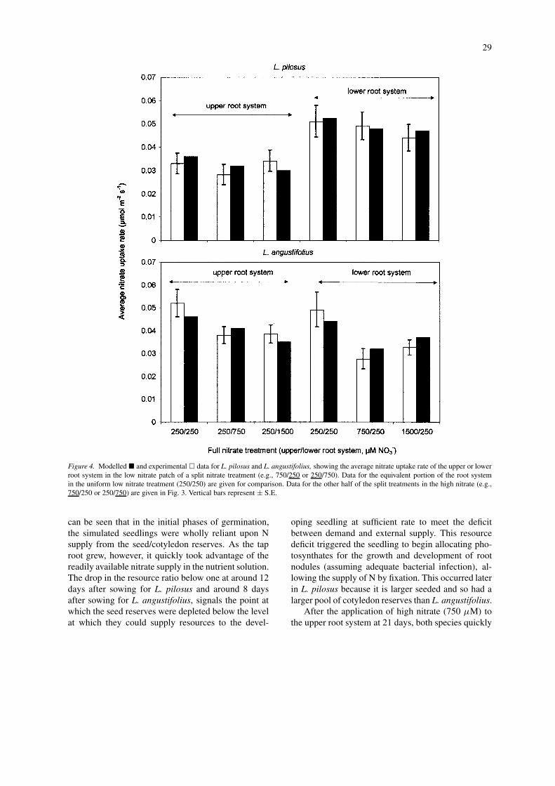
Figure 4. Modelled � and experimental � data for L. pilosus and L. angustifolius, showing the average nitrate uptake rate of the upper or lowerroot system in the low nitrate patch of a split nitrate treatment (e.g., 750/250 or 250/750). Data for the equivalent portion of the root systemin the uniform low nitrate treatment (250/250) are given for comparison. Data for the other half of the split treatments in the high nitrate (e.g.,750/250 or 250/750) are given in Fig. 3. Vertical bars represent ± S.E.

can be seen that in the initial phases of germination,the simulated seedlings were wholly reliant upon Nsupply from the seed/cotyledon reserves. As the taproot grew, however, it quickly took advantage of thereadily available nitrate supply in the nutrient solution.The drop in the resource ratio below one at around 12days after sowing for L. pilosus and around 8 daysafter sowing for L. angustifolius, signals the point atwhich the seed reserves were depleted below the levelat which they could supply resources to the devel-

oping seedling at sufficient rate to meet the deficitbetween demand and external supply. This resourcedeficit triggered the seedling to begin allocating pho-tosynthates for the growth and development of rootnodules (assuming adequate bacterial infection), al-lowing the supply of N by fixation. This occurred laterin L. pilosus because it is larger seeded and so had alarger pool of cotyledon reserves than L. angustifolius.

After the application of high nitrate (750 µM) tothe upper root system at 21 days, both species quickly

30

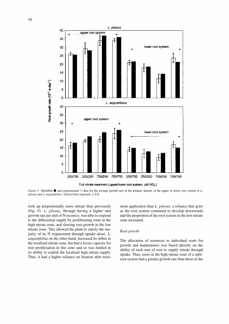
Figure 5. Modelled � and experimental � data for the average growth rate of the primary laterals of the upper or lower root system of L.pilosus and L. angustifolius. Vertical bars represent ± S.E.

took up proportionally more nitrate than previously(Fig. 9). L. pilosus, through having a higher unitgrowth rate per unit of N resource, was able to respondto the differential supply by proliferating roots in thehigh nitrate zone, and slowing root growth in the lownitrate zone. This allowed the plant to satisfy the ma-jority of its N requirement through uptake alone. L.angustifolius on the other hand, increased its influx inthe localised nitrate zone, but had a lesser capacity forroot proliferation in this zone and so was limited inits ability to exploit the localised high nitrate supply.Thus, it had a higher reliance on fixation after treat-

ment application than L. pilosus, a reliance that grewas the root system continued to develop downwardsand the proportion of the root system in the low nitratezone increased.

Root growth

The allocation of resources to individual roots forgrowth and maintenance was based directly on theability of each unit of root to supply nitrate throughuptake. Thus, roots in the high nitrate zone of a split-root system had a greater growth rate than those in the

31

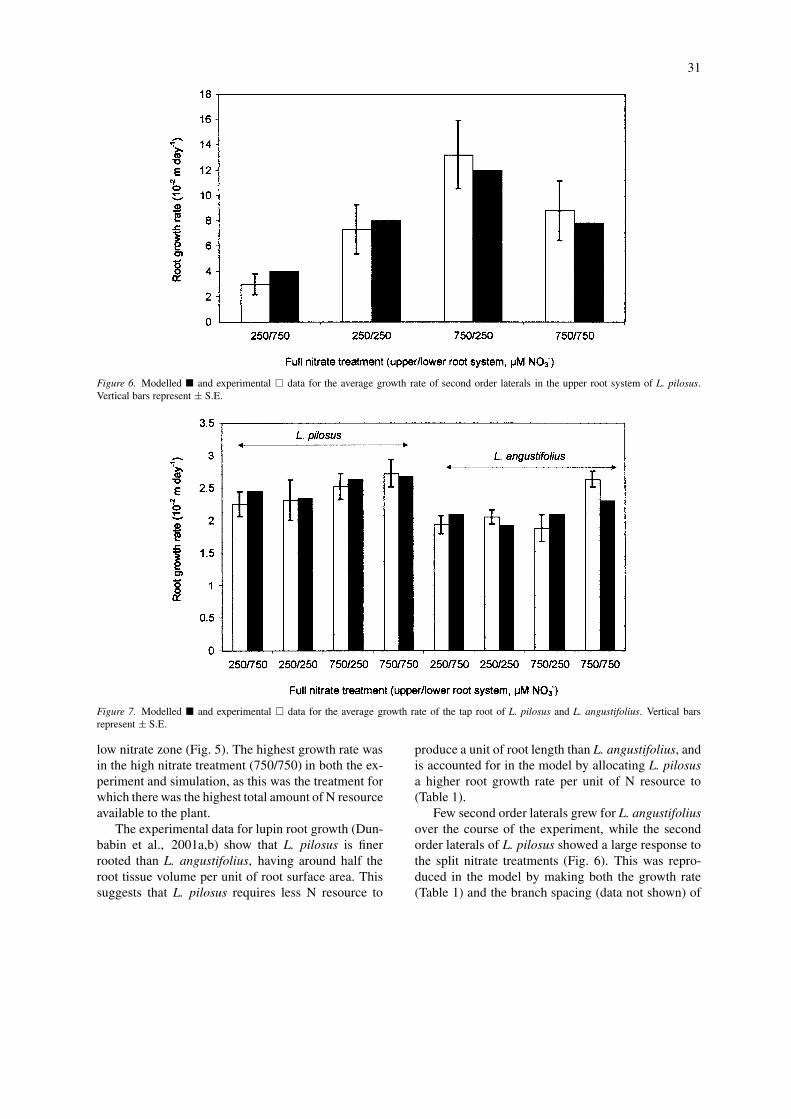
Figure 6. Modelled � and experimental � data for the average growth rate of second order laterals in the upper root system of L. pilosus.Vertical bars represent ± S.E.

Figure 7. Modelled � and experimental � data for the average growth rate of the tap root of L. pilosus and L. angustifolius. Vertical barsrepresent ± S.E.

low nitrate zone (Fig. 5). The highest growth rate wasin the high nitrate treatment (750/750) in both the ex-periment and simulation, as this was the treatment forwhich there was the highest total amount of N resourceavailable to the plant.

The experimental data for lupin root growth (Dun-babin et al., 2001a,b) show that L. pilosus is finerrooted than L. angustifolius, having around half theroot tissue volume per unit of root surface area. Thissuggests that L. pilosus requires less N resource to

produce a unit of root length than L. angustifolius, andis accounted for in the model by allocating L. pilosusa higher root growth rate per unit of N resource to(Table 1).

Few second order laterals grew for L. angustifoliusover the course of the experiment, while the secondorder laterals of L. pilosus showed a large response tothe split nitrate treatments (Fig. 6). This was repro-duced in the model by making both the growth rate(Table 1) and the branch spacing (data not shown) of

32

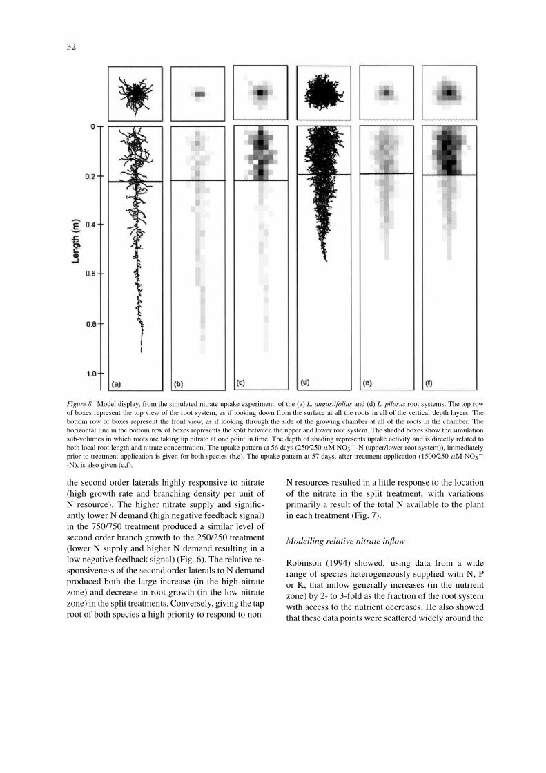
Figure 8. Model display, from the simulated nitrate uptake experiment, of the (a) L. angustifolius and (d) L. pilosus root systems. The top rowof boxes represent the top view of the root system, as if looking down from the surface at all the roots in all of the vertical depth layers. Thebottom row of boxes represent the front view, as if looking through the side of the growing chamber at all of the roots in the chamber. Thehorizontal line in the bottom row of boxes represents the split between the upper and lower root system. The shaded boxes show the simulationsub-volumes in which roots are taking up nitrate at one point in time. The depth of shading represents uptake activity and is directly related toboth local root length and nitrate concentration. The uptake pattern at 56 days (250/250 µM NO3

−-N (upper/lower root system)), immediatelyprior to treatment application is given for both species (b,e). The uptake pattern at 57 days, after treatment application (1500/250 µM NO3

−-N), is also given (c,f).

the second order laterals highly responsive to nitrate(high growth rate and branching density per unit ofN resource). The higher nitrate supply and signific-antly lower N demand (high negative feedback signal)in the 750/750 treatment produced a similar level ofsecond order branch growth to the 250/250 treatment(lower N supply and higher N demand resulting in alow negative feedback signal) (Fig. 6). The relative re-sponsiveness of the second order laterals to N demandproduced both the large increase (in the high-nitratezone) and decrease in root growth (in the low-nitratezone) in the split treatments. Conversely, giving the taproot of both species a high priority to respond to non-

N resources resulted in a little response to the locationof the nitrate in the split treatment, with variationsprimarily a result of the total N available to the plantin each treatment (Fig. 7).

Modelling relative nitrate inflow

Robinson (1994) showed, using data from a widerange of species heterogeneously supplied with N, Por K, that inflow generally increases (in the nutrientzone) by 2- to 3-fold as the fraction of the root systemwith access to the nutrient decreases. He also showedthat these data points were scattered widely around the

33

Figure 9. Behaviour of the internal parameters of the model for the 750/250 µM NO3− split treatment (grown in 250/250 µM NO3

− untiltreatment application at 21 days). The root nitrate absorption power, the fractional components of the total plant N resource and the ratio of theinternal plant N and non-N resources are given for the two species L. pilosus and L. angustifolius.

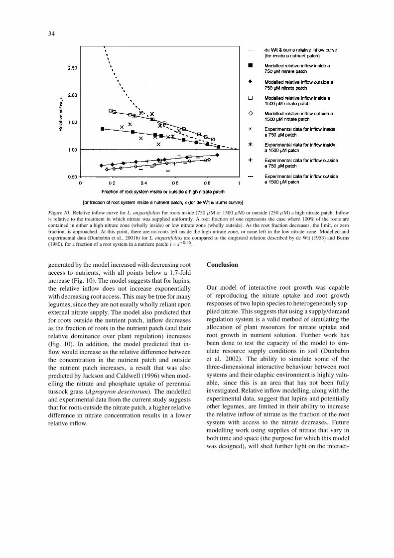
empirical relative inflow relation of de Wit (1953) andBurns (1980). This empirical relation was designedto describe the relative increase in inflow (i) that ac-companies a relative decrease in roots with access tonutrients (x), such that i=x−0.56 (Fig. 10). The inflowin the nutrient patch (with none of the target nutrientoutside the patch) is relative to the inflow when theplant is uniformly supplied with the target nutrient.While the data of Robinson (1994) show that the deWit and Burns curve provides a general description of

relative inflow over a wide collective range of species,it poorly describes the behaviour of many individualspecies (Robinson, 1994).

Few of the species studied by Robinson (1994)were legumes and none of these were tested withnitrate. The experimental data for lupins (Dunbabinet al., 2001b), with nitrate concentrations of 750 or1500µM in the nutrient patch and 250µM outside thenutrient patch, suggest that the increase in nitrate in-flow is generally around 1.5-fold (Fig. 10). The inflow

34

Figure 10. Relative inflow curve for L. angustifolius for roots inside (750 µM or 1500 µM) or outside (250 µM) a high nitrate patch. Inflowis relative to the treatment in which nitrate was supplied uniformly. A root fraction of one represents the case where 100% of the roots arecontained in either a high nitrate zone (wholly inside) or low nitrate zone (wholly outside). As the root fraction decreases, the limit, or zerofraction, is approached. At this point, there are no roots left inside the high nitrate zone, or none left in the low nitrate zone. Modelled andexperimental data (Dunbabin et al., 2001b) for L. angustifolius are compared to the empirical relation described by de Wit (1953) and Burns(1980), for a fraction of a root system in a nutrient patch: i = x−0.56.

generated by the model increased with decreasing rootaccess to nutrients, with all points below a 1.7-foldincrease (Fig. 10). The model suggests that for lupins,the relative inflow does not increase exponentiallywith decreasing root access. This may be true for manylegumes, since they are not usually wholly reliant uponexternal nitrate supply. The model also predicted thatfor roots outside the nutrient patch, inflow decreasesas the fraction of roots in the nutrient patch (and theirrelative dominance over plant regulation) increases(Fig. 10). In addition, the model predicted that in-flow would increase as the relative difference betweenthe concentration in the nutrient patch and outsidethe nutrient patch increases, a result that was alsopredicted by Jackson and Caldwell (1996) when mod-elling the nitrate and phosphate uptake of perennialtussock grass (Agropyron desertorum). The modelledand experimental data from the current study suggeststhat for roots outside the nitrate patch, a higher relativedifference in nitrate concentration results in a lowerrelative inflow.

Conclusion

Our model of interactive root growth was capableof reproducing the nitrate uptake and root growthresponses of two lupin species to heterogeneously sup-plied nitrate. This suggests that using a supply/demandregulation system is a valid method of simulating theallocation of plant resources for nitrate uptake androot growth in nutrient solution. Further work hasbeen done to test the capacity of the model to sim-ulate resource supply conditions in soil (Dunbabinet al. 2002). The ability to simulate some of thethree-dimensional interactive behaviour between rootsystems and their edaphic environment is highly valu-able, since this is an area that has not been fullyinvestigated. Relative inflow modelling, along with theexperimental data, suggest that lupins and potentiallyother legumes, are limited in their ability to increasethe relative inflow of nitrate as the fraction of the rootsystem with access to the nitrate decreases. Futuremodelling work using supplies of nitrate that vary inboth time and space (the purpose for which this modelwas designed), will shed further light on the interact-

35

ive relationship between lupin root systems and nitrateuptake from the soil profile.

Acknowledgements

This study was supported by the Grains Researchand Development Corporation through a postgraduatescholarship held by the senior author.

References

Addiscott T M 1996 Measuring and modelling nitrogen leaching:parallel problems. Plant Soil 181, 1–6.

Addiscott T M and Wagenet R J 1985 Concepts of solute leaching insoils: a review of modelling approaches. J. Soil Sci. 36, 411–424.

Anderson G C, Fillery I R P, Dolling P J and Asseng S 1998aNitrogen and water flows under pasture-wheat and lupin-wheatrotations in deep sands in Western Australia. 1. Nitrogen fixationin legumes, net N mineralisation and utilisation of soil-derivednitrogen. Aust. J. Agric. Res. 49, 329–343.

Anderson G C, Fillery I R P, Dunin F X, Dolling P J and Asseng S1998b Nitrogen and water flows under pasture-wheat and lupin-wheat rotations in deep sands in Western Australia. 2. Drainageand nitrate leaching. Aust. J. Agric. Res. 49, 345–361.

Baldwin J P 1976 Competition for plant nutrients in soil; a theoret-ical approach. J. Agric. Sci. (Cambridge) 87, 341–356.

Baldwin J P, Nye P H and Tinker P B 1973 Uptake of solutes bymultiple root systems from soil. III. A model for calculating thesolute uptake by a randomly dispersed root system developing ina finite volume of soil. Plant Soil 38, 621–635.

Bingham I J, Blackwood J M, Stevenson E A 1997 Site, scale andtime-course for adjustments in lateral root initiation in wheatfollowing changes in C and N supply. Ann. Bot. 80, 97–106.

Bloom A J, Chapin F S and Mooney H A 1985 Resource limitationin plants — an economic analogy. Ann. Rev. Ecol. Syst. 16, 363–392.

Burns I G 1980 Influence of the spatial distribution of nitrate on theuptake of N by plants: A review and a model for rooting depth.J. Soil Sci. 31, 155–173.

Clarkson D T and Lüttge U 1991 Inducible and repressible nutrienttransport systems. Prog. Bot. 52, 61–83.

Clements J C, While P F and Buirchell B J 1993 The root mor-phology of Lupinus angustifolius in relation to other Lupinusspecies. Aust. J. Agric. Res. 44, 1367–1375.

Cowie A L, Jessop R S, MacLeod D A and Davis G J 1990a Effectof soil nitrate on the growth and nodulation of lupins (Lupinusangustifolius and L. albus). Aust. J. Agric. Res. 30, 655–659.

Cowie A L, Jessop R S and MacLeod D A 1990b Effect of soilnitrate on the growth and nodulation of winter crop legumes.Aust. J. Exp. Agric. 30, 651–654.

de Willigen P 1991 Nitrogen turnover in the soil-crop system; com-parison of fourteen simulation models. Fertil. Res. 27, 141–149.

De Wit C T 1953 A physical theory on the placement of fertilisers.Versl. Landbouwk. Onderz. 59, 1–71.

Diggle A J 1988a ROOTMAP — a model in three-dimensionalcoordinates of the growth and structure of fibrous root systems.Plant Soil 105, 169–178.

Diggle A J 1988b ROOTMAP2.1 — A root growth simulationprogram. Miscellaneous publication No. 6188, Department ofAgriculture Western Australia, Western Australia.

Diggle A J 1988c ROOTMAP — A root growth model. Math.Comput. in Simulation 30, 175–180.

Diggle A J 1990 Interaction between mineral nitrogen and growthof wheat roots in a leaching environment. PhD, The Universityof Western Australia, Perth.

Drew M C 1975 Comparison of the effects of a localised supply ofphosphate, nitrate, ammonium and potassium on the growth ofthe seminal root system, and the shoot, in barley. New Phytol.75, 479–490.

Drew M C and Saker L R 1975 Nutrient supply and the growth ofthe seminal root system in barley. II. Localised compensatoryincreases in lateral root growth and rates of nitrate uptake whennitrate supply is restricted to only one part of the root system. J.Exp. Bot. 26, 79–90.

Drew M C and Saker L R 1978 Nutrient supply and the growth ofthe seminal root system in barley. J. Exp. Bot. 29, 435–451.

Drew M C, Saker L R and Ashley T W 1973 Nutrient supply andthe growth of the seminal root system in barley. I. The effect ofnitrate concentration on the growth of axes and laterals. J. Exp.Bot. 24, 1189–1202.

Dunbabin V, Rengel Z and Diggle A 2001a The root growthresponse to heterogeneous nitrate supply differs for Lupinus an-gustifolius and Lupinus pilosus. Aust. J. Agric. Res. 52, 495–503.

Dunbabin V, Rengel Z and Diggle A 2001b Lupinus angustifoliushas a plastic uptake response to heterogeneously supplied nitratewhile Lupinus pilosus does not. Aust. J. Agric. Res. 52, 505–512.

Dunbabin V, Diggle A and Rengel Z 2002 Simulation of field databy a basic three-dimensional model of interactive root growth.Plant Soil. 239, 39–54.

Evans J, O’Connor G E, Turner G L and Bergersen F J 1987 Influ-ence of mineral nitrogen on nitrogen fixation by lupin (Lupinusangustifolius) as assessed by 15N isotope dilution methods. FieldCrops Res. 17, 109–120.

Feddes R A, Kowalik P, Kolinska-Mayinka K and Zaradny H 1976Simulation of field water uptake by plants using a soil waterdependent root extraction function. Hydrology 31, 13–26.

Fitter A H and Stickland T R 1991 Architectural analysis of plantroot systems. 2. Influence of nutrient supply on architecture incontrasting plant species. New Phytol. 118, 383–389.

Fitter A H, Nichols R and Harvey M L 1988 Root system architec-ture in relation to life history and nutrient supply. Funct. Ecol. 2,345–351.

Gersani M and Sachs T 1992 Development correlations betweenroots and heterogeneous environments. Plant Cell Environ. 15,463–469.

Habib R and Lafolie F 1991. Water and nitrate redistribution insoil as affected by root distribution and absorption. In PlantRoot Growth — an Ecological Perspective. Ed. D Atkinson. pp.131–145. Blackwell Scientific Publications, Oxford.

Hamblin AP and Hamblin J 1985 Root characteristics of sometemperate legume species and varieties on deep, free-drainingentisols. Aust. J. Agric. Res. 36, 63–72.

Hamblin A and Tennant D 1987 Root length density and water up-take in cereals and grain legumes: How well are they corelated?Aust. J. Agric. Res. 38, 513–527.

Jackson R B and Caldwell M M 1996 Integrating resource het-erogeneity and plant plasticity: modelling nitrate and phosphateuptake in a patchy soil environment. J. Ecol. 84, 891–903.

Lambers H, Chapin F S and Pons T L 1998 Plant PhysiologicalEcology. pp. 249–251. Springer, New York.

Lim J T, Wilkerson G G, Raper C D Jr and Gold H J 1990 Adynamic growth model of vegetative soya bean plants: modelstructure and behaviour under varying root temperature andnitrogen concentration. J. Exp. Bot. 41, 229–241.

36

Lynch J P, Nielsen K L, Davis R D and Jablokow A G 1997 Sim-Root: Modelling and visualization of root systems. Plant Soil188, 139–151.

Nye P H and Tinker P B 1977 Solute movement in the soil-rootsystem. Oxford, 110 p.

Nye P H, Brewster J L and Bhat K K S 1975 The posibilityof predicting solute uptake and plant growth response fromindependently measured soil and plant characteristics. I. Thetheoretical basis of the experiments. Plant Soil 42, 161–170.

Pagès L 1999 Root system architecture: from its representation tothe study of its elaboration. Agronomie 19, 295–304.

Pagès L, Jourdan M O and Picard D 1989 A simulation model of thethree-dimensional architecture of the maize root system. PlantSoil 119, 147–154.

Probert M E, Dimes J P, Keating B A, Dalal R C and Strong W M1998 APSIM’s water and nitrogen modules and simulation of thedynamics of water and nitrogen in fallow systems. Agric. Syst.56, 1–28.

Raper C D Jr, Osmond D L, Wann M and Weeks W W 1978 Inter-dependence of root and shoot activities in determining nitrogenuptake rate of roots. Bot. Gaz. 139, 289–294.

Richards L A 1931 Capillary conduction of liquids through porousmediums. Physics 1, 318–333.

Robinson D 1994 The responses of plants to non-uniform suppliesof nutrients. New Phytol. 127, 635–674.

Robinson D 1996 Variation, co-ordination and compensation in rootsystems in relation to soil variability. Plant Soil 187, 57–66.

Rose C W, Chichester F W, Williams J R and Ritchie J T 1982aA contribution to simplified models of field solute transport. J.Environ. Qual. 11, 146–150.

Rose C W, Chichester F W, Williams J R and Ritchie J T 1982b Ap-plication of an approximate analytic method of computing soluteprofiles with dispersion in soils. J. Environ. Qual. 11, 151–155.

Somma F, Hopmans J W and Clausnitzer V 1998 Transient three-dimensional modeling of soil water and solute transport withsimultaneous root growth, root water and nutrient uptake. PlantSoil 202, 281–293.

Thaler P and Pagès L 1998 Modelling the influence of assimilateavailability on root growth and architecture. Plant Soil 201, 307–320.

Thornley J H M 1972 A balanced quantitative model for root:shootratios in vegetative plants. Ann. Bot. 36, 431–441.

White PF 1990 Soil and plant factors relating to the poor growth ofLupinus species on fine-textured, alkaline soils — a review. Aust.J. Agric. Res. 41, 871–890.

Zhang H and Forde B G 1998 An Arabidopsis MADS box gene thatcontrols nutrient-induced changes in root architecture. Science279, 407–409.

Section editor: R. Aerts

Appendix 1.

Symbols

a Root radius (m)

b Buffer power of soil (dC/dCl ) (unitless)

b Parameter coefficient for a sigmoid curve (unitless)

Bi Branching density of section of root i (branches m−1)

C̄1 Average concentration of solute in solution (mol m−3)

Cla Soil solution solute concentration at the root surface (mol m−3)

D Diffusion coefficient of solute in soil (m2s−1)

Dfix Plant demand for N supply by fixation (mol N plant−1)

DNroots, DNshoots N demand of the root and shoot systems (mol N plant−1)

Dw Unsaturated hydraulic diffusivity (m2 s−1)

Ew Evaporation rate of water from the soil surface (m3 m−2s−1)

Emax Potential evaporation rate (m3 m−2s−1)

F Frequency of occurrence of a displaced ion (normal distribution function with a mean of � and a

variance of 2(�ε) (m−1)

FD Diffusive flux of solute (mol m−2 s−1)

Fmax Maximum flux into the root (mol m−2 s−1)

Gi Growth rate of section of root i (m s−1)

i Section of root i, such that the entire root system (of size n) is described by the sum of all root

sections from i = 1 to i = n (unitless)

k Kinetic parameter for a sigmoid curve (m−1)

Km Michaelis–Menten kinetic constant (mol m−3)

L Root length density (m m−3)

Mnod Cost of nodule maintenance (mol plant−1)

N, nN Nitrogen (mol N plant−1) and non-nitrogen resources (mol nN plant−1)

Nfix N resource supplied by fixation (mol N plant−1)

Nm, nNm Total N and non-N mobile resource pools (mol plant−1)

Nroots N resource supplied to the root system (mol N plant−1)

37

Appendix 1 Continued

Symbols

Ns, nNs Stored N and non-N resource pools (mol plant−1)

Nseed, nNseed Supply of N or non-N resources by the seed/cotyledon reserves (mol plant−1)

Nuptake, nNuptake Supply of N or non-N resources through uptake by the root system (mol plant−1)

p Plant cover factor (unitless)

q Water flux (m s−1)

R Ratio of resources within the plant

Rfd Resources supplied to the nodules based on the fixation demand (mol plant−1)

Rfix Resources supplied for nodule maintenance based on the current contribution of fixation to the total

N supply (mol plant−1)

rLL Lower limit of the whole plant demand system capacity to reduce the net influx of a resource (unitless)

Rnod Total resource supply to the nodules (mol plant−1)

RrNi, RrnNi Resources supplied to section of root i based upon return of N or non-N to the plant (mol)

Rroots Total resource supply to the root system (mol plant−1)

S Supply ratio of resources to the plant from the root system

Sw Water uptake rate (m3 m−3 s−1)

t Time (s)

Tb Branching lag time (s)

Tmax Potential rate of transpiration (m3 m−1 s−1)

v Soil solution volume (m3)

w Water flux at root surface (m s−1)

x (1/√πL), radius of the soil volume exploited by the root (dC/dr = 0) (m)

z A position below the original location of the ion (m)

x, y, z Position coordinates in three–dimensional space (m)

αavg Absorption coefficient averaged over the whole root system (m s−1)

αi Actual absorption coefficient of N or non-N for each unit of root i (m s−1)

αli Local absorption coefficient for each unit of root i (m s−1)

αw Weighting function for water uptake, describes the plants’ ability to extract water from the soil profile as a function

of the soil water potential (unitless)

χnod Number of nodules

δ Change in the size of a resource over time increment δt

� Peak displacement = the amount of water that has moved passed the ion (m)

� Vector operator (m−1)

ε Displacement dependent dispersivity (m)

µg Unit root growth rate in response to N or non-N resources = f(branch order) (m mol−1 s−1)

µb Unit root branching density in response to N or non-N resources = f(branch order) (m mol−1 s−1)

µfix Unit fixation rate (branches m−1 mol−1)

µnodg Unit nodule growth rate (nodules mol−1)

µnodm Unit nodule maintenance cost (mol plant−1 nodule−1)

µseedN,µseednN Unit supply rate of N or non-N resources from the seed/cotyledon (mol plant−1 s−1)

θ Volumetric water content (m3 m−3)

ω Down regulation factor, and uptake activity lower limit (LL) or upper limit (UL) for N (ωN) or non-N (ωnN)

resources (unitless)

ψ Soil water potential (m)

q = −Dw � θ (1)

Sw = Tmaxαw(�)L(x, y, z) (2)

αw = 1

1 + bexp(−k�) (3)

Ew = p(t)Emax(t)αw(�) (4)

38

F = 1√2π(2(�ε))

e−((z−�)22(2(�ε))

)(5)

FD = −D � C (6)

dC̄li

dt= −2πaiαiLi

b

× C̄li

αiwi

+(

1 − αiwi

)(2

2− aiwiDb

)(( xa )

2−(aiwi/Db)i −1

( xa)2i−1

)(7)

δNm = δNuptake + δNfix + δNseed =(n∑i=1

(δCli)vi

)+ xnodµfixδt + δNseed (8)

δnNm = δnNuptake + δnNseed (9)

δNseed or δnNseed = the lesser of

µseedNδt or µseednNδt (seed supply rate),

or plant demand for N or nN resources (10)

αli (t) =(

Fmax

Km + Clai

)1

ω(11)

S(t) = αavg

αli; ωLL ≤ S ≥ ω (12)

rLL ≤ R(t);R ∗ S ≤ ωUL (13)

αi(t) = R(t) ∗ S(t) ∗ αli (t) (14)

DNroots : DNshoots = f (t) (15)

If demand is less than supply :Nroots = DNroots;(DNroots +DNshoots) ≤ (Nm +Ns)

otherwise :Nroots = [DNroots/(DNroots +DNshoots)] ∗(Nm +Ns);(DNroots +DNshoots) ≥ (Nm +Ns) (16)

Ns(t) = (Nm +Ns)(t−δt) − (Nroots + Nshoots)(t−δt)(17)

Rroots = Nroots + nNroots (18)

RrNi =((Nuptake)i

Nuptake

)∗ Rroots (19)

Gi = µgN(RrNi )+ µgnN(RrnNi ) (20)

Bi = µbN(RrNi )+ µbnN(RrnNi ) (21)

Rnod = Rfix + Rfd (22)

Rfix =(

Nfix

Nm +Ns

)∗ γ ∗ Rroots (23)

Rfd = [(γ ∗ Rroots)− Rfix] ∗Dfix (24)

Mnod = µnodm ∗ χnod (25)

δχnod = µnodg ∗ (Rnod −Mnod) (26)

χnod(t) = χnod(t−δt) + δχnod (27)