modelling the full costs of an intermodal and road freight transport network

Transportation Research Part D 12 (2007) 33–44

www.elsevier.com/locate/trd

Modelling the full costs of an intermodal and roadfreight transport network

Milan Janic *

OTB Research Institute, Delft University of Technology, Thijsseweg 11, 2629 JA, Delft, The Netherlands

Abstract

This paper develops a model for calculating comparable combined internal and external costs of intermodal and roadfreight transport networks. Internal costs consist of the operational-private costs borne by the transport and intermodalterminal operators, and the time costs of goods tied in transit. The external costs include the costs of the impacts of bothnetworks on society and the environment such as local and global air pollution, congestion, noise pollution, and trafficaccidents. The model is applied to the simplified configurations of both networks using the inputs from the Europeanfreight transport system. The objective is to investigate some effects of European Union policy, which aims to internalisethe external costs of transport, on the prospective competition between two networks from a social perspective.� 2006 Elsevier Ltd. All rights reserved.

Keywords: Intermodal freight transport; Networks; Full costs; Externalities; Modal; Competition

1. Introduction

Intermodal freight transport provides transport for consolidated loads such as containers, swap-bodies andsemi trailers by combining at least two modes (European Commisson, 2002). In Europe, intermodal freighttransport has frequently been seen as a potentially strong competitor to road transportation and to be environ-mentally friendlier in many contexts.1 Its development to date, however, has not confirmed such expectations.For example, during 1990–1999, European intermodal freight transport grew steadily from an annual volumeof about 119 to about 250 billion t–km2 with an increase in its market share volumes from about 5%–9%.3

1361-9209/$ - see front matter � 2006 Elsevier Ltd. All rights reserved.

doi:10.1016/j.trd.2006.10.004

* Tel.: +31 015 278 1899; fax: +31 015 278 3450.E-mail address: [email protected]

1 Efforts to promote intermodal freight transport have increased over the past two decades (Bontekoning et al., 2004; EuropeanCommisson, 1999; European Conference of Ministers of Transport, 1998). Competitiveness of intermodal transport were investigated(European Commisson, 2001a,b; Morlok et al., 1995).

2 About 91% of this total was international. Rail carried about 20%, inland waterways 2%, and short-sea shipping 78% of theinternational traffic, while about 97% of the domestic traffic was carried out by rail and 3% by inland waterways.

3 Freight transport in Europe was grew by an average annual rate of 2% during the period 1970–2001 and reached about 3000 billionst–km (tonne–kilometres) in 2001, of which about 44% was carried by road, 41% by coastal shipping, 8% by rail, and 4% by inlandwaterways.

mailto:[email protected]

34 M. Janic / Transportation Research Part D 12 (2007) 33–44

This was mainly due to enhancement of operations in Trans-European corridors of 900–1000 km that carriedabout 10% of the tonnage. During the same period, in corridors of 200–600 km the share of intermodal transportwas only about 2%, and 2%–3% in terms of the volumes of t–km and in tonnes, respectively. Since 1999 themarket share has not really improved, mostly due to a low containerisation rate, deterioration in the qualityof services of intermodal transport, and improvements in the efficiency and quality of road transport services(European Commisson, 1999, 2000, 2001a, 2002; UIRR, 2000).

This paper analyses the internal and external costs of an intermodal and an equivalent road transport net-work to investigate European Union (EU) policies intended to internalise negative externalities.

2. The intermodal and road freight transport network

Analysis of the full costs of a given intermodal and equivalent road transport network requires an under-standing of the network size, of the intensity of operations, of the technology in use, and of the internal andexternal costs of individual components of the system. Both networks are assumed of equivalent size in termsof the spatial coverage, number of nodes and the volumes of demand they serve. Fig. 1 shows a simplifiedscheme.

Network nodes are the origins and destinations of goods. They represent clusterings of manufacturingplants, warehouses, logistics centres and/or freight terminals located in shipper and receiver areas. The spatialconcentrations shippers and recipients are divided into zones. Intermodal terminals are also nodes but only forthe short-term storage and/or direct transferring of goods. Goods flows in both networks are consolidated tobe by standardized units – containers, swap-bodies and semi-trailers.

Transport infrastructure provides the means for movement of the freight units. The nature of this infra-structure and the quality of service it offers depends on the volume of demand, the efficiency and effectivenessof the services, and the physical scale of the hardware.

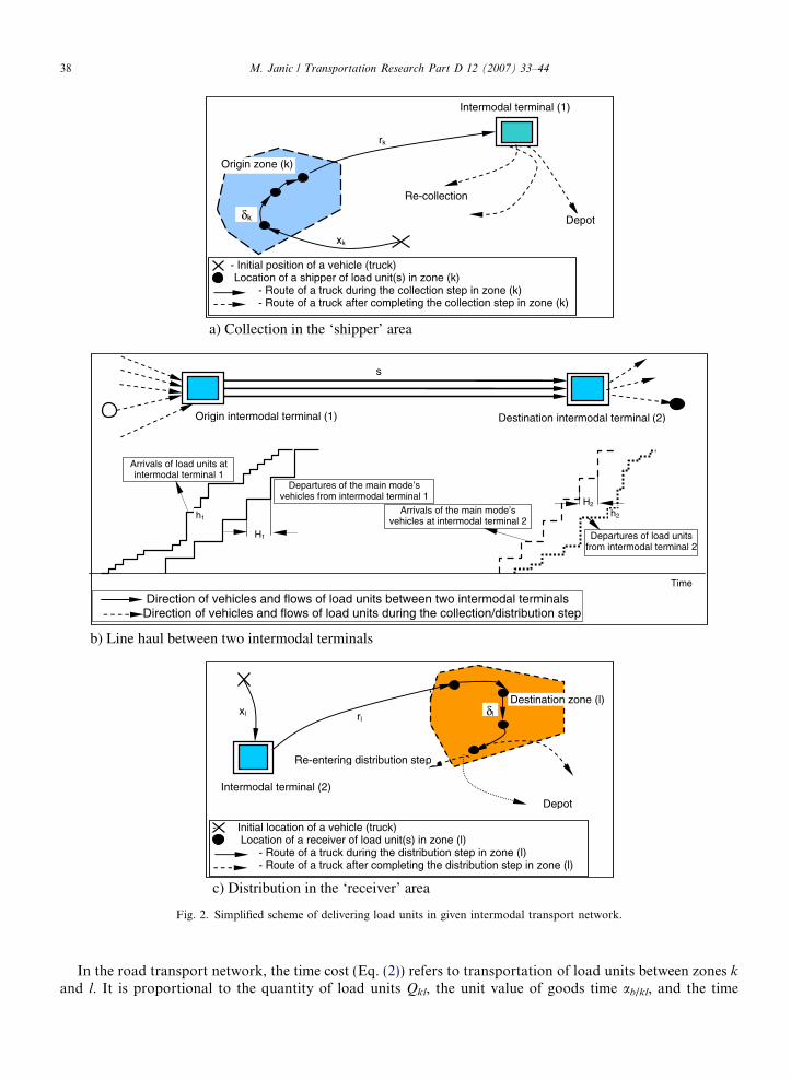
Intermodal transport involves a number of stages: (i) collection in the originating zone and transportationby truck to the origin intermodal terminal located in the shipper area; (ii) transhipment at the origin inter-modal terminal from truck to the trunk-haul, non-road transport mode (rail, inland waterways, air); (iii)line-haul transportation between the origin and destination intermodal terminals by the trunk-haul mode;(iv) transhipment at the destination intermodal terminal in the receiver area from the trunk-haul mode to

1

2

3

k

K-31

2

l

L-2

K-2

- Origins of load units – shippers - Destinations of load units - receivers - Intermodal terminals - Intermodal transport links - Equivalent road transport links

T1

T2

‘Receiver’s area

K

K-1

L-1

L

»

‘Shipper’s area

Fig. 1. Simplified scheme of an intermodal and road freight transport network.

M. Janic / Transportation Research Part D 12 (2007) 33–44 35

trucks; (v) distribution from the destination intermodal terminal to the destination zone by truck (EuropeanCommisson, 2000).

In the road transport network movement of loads between shippers and receivers is carried out directly bythe same truck in three steps: collection in the origin zones; line-hauling from the border of the origin to theborder of the destination zone; and distribution within the destination zones (Daganzo, 1999).

There are internal and external costs associated with a movement through an intermodal system and itsequivalence by a road transport network. Internal costs comprise the operators’ costs of moving units betweenshippers and receivers. The external costs are costs that networks impose on society, including environmentalcosts. Both categories of cost can be specified for each stage in the networks. They generally depend on thenetwork nature, characterised by its location, distances and number of nodes; the intensity of activities inthe network characterised its use; the efficiency of services, and the prices of inputs. Particularly relevantfor external costs are the emission rates of pollutants and the number of accidents, and their impacts on soci-ety and the environment. In addition, network services can impose delays on other traffic by creatingcongestion.

2.1. Internal costs

The collection, distribution, line hauling and transhipment of units moved within intermodal system deter-mine the internal costs of the network. The cost of each component embraces the cost of ownership, insurance,repair and maintenance, labour, energy, taxes, and tolls/fees paid for using the network. The network infra-structure and mobile plant are assumed to be in place to serve a given volume of demand given the efficiency ofthe system. Thus, the costs of investment in any additional infrastructure and/or rolling stock are not takeninto account.

The internal costs of an equivalent road transport network are analogous to those of the road part of theintermodal network plus the collection and delivery parts of the system. The internal costs directly associatedwith the particulars of a consignment, such as depreciation, maintenance, repair, and insurance costs, are notincluded because they are assumed to be borne by shippers or recipients (European Commisson, 2001a,b;Levison et al., 1996).

2.2. External costs

Because of a lack of full property bright allocation, each step of the door-to-door delivery operation ineither network generates burdens on society. If intensive and persistent, these burdens if not reflected in pricesare considered as the external costs. As they are not internalised, the external costs are usually estimated indi-rectly using such methods as willingness-to-pay for avoiding, mitigating or controlling particular impacts. Theexternal costs of both networks embrace the cost of damages by burdens such as the local and global air pol-lution, congestion, noise, and traffic accidents.

2.3. Intermodal network

• Air pollutionTrucks carrying out collection and distribution usually burn diesel fuel and cause air pollution, the partic-ular components of which can cause locally damage to surrounding buildings, green areas, and people’shealth. However, if deposited by weather in remote locations this air pollution can also have a widerimpact. Air pollution from the main transport mode during the line haul between intermodal terminalsdepends on the type of energy used by mode. If aircraft, rail diesel engines, and/or diesel-powered ships(barges) are used the air pollution is direct. If electric energy is used, as by some railways, the air pollutionis indirect, dependent on the composition of sources from which the electric energy is obtained. These areusually the remote power plants considered as the point sources of local air pollution.The air pollution gen-erated by the operations of intermodal terminals is mainly indirect because the electric energy remote plantsis used for the cranes transhipping the loads.


• CongestionThe trucks performing the collection and distribution of load units usually move in the densely urbanisedand/or industrialised zones. They may experience congestion and the consequent private delays. However,they may also impose delays on other vehicles whose costs are counted as an externality. The inter-terminaltransport mode is assumed to be free of congestion. Thus introducing new services does not cause shifting orrescheduling of existing ones and service-departures do not interfere and impose delays on each other. Loadsare also assumed not to impose delay costs on each other while being handled in the intermodal terminals.

• NoiseTrucks involved in the collection and distribution of loads generate noise, which, if it exceeds tolerable lim-its causes annoyance and if it persistent can cause a decline productivity and have adverse health effects.Noise generated by line hauling between two intermodal terminals can have similar effect. Noise fromthe intermodal terminals is not considered since it is assumed to be just a part of ambient urban noise.

• Traffic accidentsTraffic accidents cause damage and property loss the network operators and third parties, in addition to theloss of life and injuries to the affected people. They are considered separately for each step and transportmode of the intermodal transport network due to the different frequency, character of occurrence, and con-sequences. Accidents at the intermodal terminals are not considered since are very rare events.

2.4. Road network

The same categories of external costs and ways of their consideration are used for the three operationalsteps of the road transport network. Specifically, particular burdens, damages, and associated costs are con-sidered regarding the use of diesel-powered trucks along the entire door-to-door distance.

3. Modelling full costs

Modelling the full costs of an intermodal and equivalent road transport network involves developing themodel, collection of data, and the model application. Developing the model includes identification of the rel-evant variables and their relationships. The variables reflect the type and format of data needed for the modelapplication. Data collection is particularly challenging.

External costs are estimated using a four-stage process, starting with the quantification of emissions/burdens and estimation of their spatial concentration, proceeding with an estimation of the prospectivedamages, and ending with putting monetary values on short and long-term damage. In both networks, dataon the internal and external costs refer to particular parts (segments, actors) operating under different techni-cal/technological, market, and environmental-spatial conditions. The results are then aggregated.

The model is based on a set of assumptions:

3.1. Intermodal network

• Collection and distribution– Vehicles of the same capacity and load factor collect and/or distribute load units in a given zone.– Each vehicle makes a round trip of approximately the same length at a constant average speed.– The collection step starts from the vehicle’s initial position, which can be anywhere within the ‘shipper’ area

and ends at the origin’s intermodal terminal. The distribution step starts from the destination intermodalterminal where the vehicles may be stored in a pool and ends in the reception area at the last receiver.

– Headways between the arrivals and departures of the successive vehicles (and thus loads) at the originand from the destination intermodal terminal, respectively, are approximately constant and independentof each other.

• Line-haul between two terminals– Headways between successive departures of the main mode’s vehicles between two intermodal terminals

are constant, reflecting the practice of many non-road transport operators in Europe to schedule regularweekday services.

– The each inter-terminal vehicle has identical capacity irrespective of whether it is rail or road.– The average speed and the anticipated delays of the main mode are constant and approximately equal.


3.2. Road network

• Trucks of similar capacity and load factor transport units between the origin and destination zones.• Units are loaded onto each truck for exclusively one given pair of ‘zones’. The area, layout and distance

between particular shippers and receivers in particular ‘zones’ crucially influence the length of vehicle tourdistances. The vehicle speed is constant.

• The trucks move between the borders of particular pairs of the origin and destination zones along the sameroutes at a constant line-haul speed.

Based on these assumptions, the generic structure for calculating particular cost categories (internal, exter-nal) and cost type (transport, time, handling, type of externality) for particular steps of operation of the net-works is developed:

• Internal cost:

Transport cost ¼ ðFrequencyÞ � ðCost per frequencyÞ¼ ½ðDemandÞ=ðLoad factor� Vehicle capacityÞ� � ðCost per frequencyÞ; ð1Þ

Time cost ¼ ðDemandÞ � ðTimeÞ � ðCost per unit of time per unit of demandÞ; ð2ÞHandling cost ¼ ðDemandÞ � ðCost per unit of demandÞ: ð3Þ

• External cost:

External cost ¼ ðFrequencyÞ � ðExternal cost per frequencyÞ¼ ½ðDemandÞ=ðLoad factor� Vehicle capacityÞ� � ðExternal cost per frequencyÞ: ð4Þ

The variables in Eq. (1) are specific for particular steps in the intermodal network. In the collection anddistribution step, ‘frequency’ relates to the number of vehicle runs needed to collect and/or distribute a givenvolume of units. In zone k, ‘frequency’ fk is proportional to the volume of units Qk and inversely proportionalto the product of truck capacity Mk and load factor kk. ‘Cost/frequency’ relates to the cost of individual trucktypes and is expressed in relation to distance of a trip as cok(dk). Distance dk includes the segments between thevehicle’s initial position and the first stop xk, the average distances between successive stops dk, and the dis-tance between the last stop and the intermodal terminal rk (Fig. 2(a)). The reasoning for the trip frequenciesand distances can also be applied to the distribution step (Fig. 2(c)). For the line hauling step, f is proportionalto the volume of units in network Q, and inversely proportional to the product of the modular capacity of theinter-terminal mode its load factor (Fig. 2(b)). It is determined so as to minimise the internal and external costsfor the transport operator and the time cost of loads while in the network (Daganzo, 1999). The internal andexternal cost per departure, c(w, s) and ce(w, s), depend on the vehicle weight w and the line-hauling distance s.The cost of time of loads at both intermodal terminals and line hauling step ab1, ab2,and ab1, respectively,depends on the value of goods and the relevant discount rate. For the road transport network, the variablesin the Eq. (1) have an analogous meaning, reflecting that trucks cover the entire door-to-door distancebetween ‘zones’ k and l.

The variables in Eq. (2) have the following meaning: In the intermodal transport network the time cost inthe collection step in zone k is proportional to the quantity of load units Qk, the unit value of goods time ak,and the time of the vehicle tour tk, which is proportional to the length of tour dk and the average vehicle speedvk. In the line-hauling step the time cost is proportional to the waiting and line haul time, and their unit costs.The line haul time is proportional to the distance s and anticipated delays D and inversely proportional to thevehicle speed vs. The time cost is determined by optimizing the total costs of the line-hauling step with respectto the departure frequency of the main transport mode.

a) Collection in the ‘shipper’ area

c) Distribution in the ‘receiver’ area

δl

Destination zone (l)xl rl

Intermodal terminal (2)

- Initial location of a vehicle (truck) - Location of a receiver of load unit(s) in zone (l)

- - Route of a truck during the distribution step in zone (l)- Route of a truck after completing the distribution step in zone (l)

Depot

Re-entering distribution step

xk

δk

rk

Intermodal terminal (1)

Origin zone (k)

- Initial position of a vehicle (truck) - Location of a shipper of load unit(s) in zone (k)

- - Route of a truck during the collection step in zone (k) - - Route of a truck after completing the collection step in zone (k)

Re-collection

Depot

Direction of vehicles and flows of load units between two intermodal terminals Direction of vehicles and flows of load units during the collection/distribution step

s

Destination intermodal terminal (2)Origin intermodal terminal (1)

Departures of the main mode’s vehicles from intermodal terminal 1

Arrivals of the main mode’s vehicles at intermodal terminal 2

Departures of load units from intermodal terminal 2

Arrivals of load units at intermodal terminal 1

Time

H1

h1 h2

H2

b) Line haul between two intermodal terminals

Fig. 2. Simplified scheme of delivering load units in given intermodal transport network.


In the road transport network, the time cost (Eq. (2)) refers to transportation of load units between zones k

and l. It is proportional to the quantity of load units Qkl, the unit value of goods time ab/kl, and the time

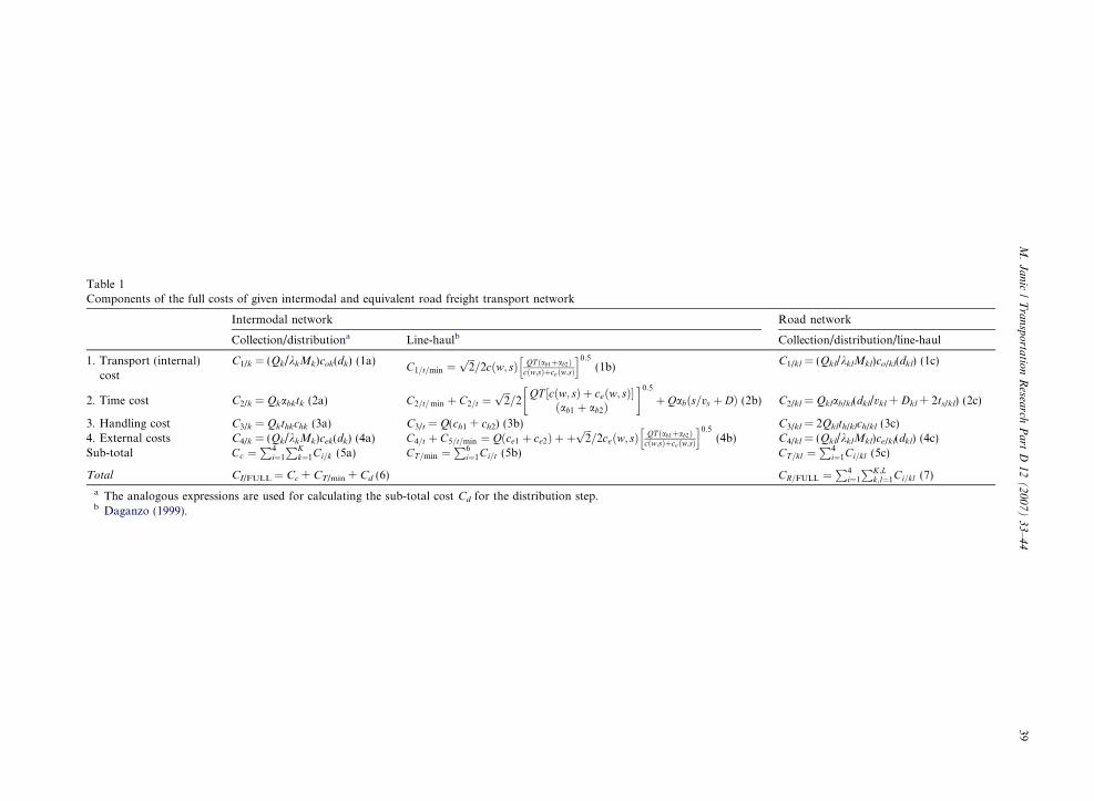
Table 1Components of the full costs of given intermodal and equivalent road freight transport network

Intermodal network Road network

Collection/distributiona Line-haulb Collection/distribution/line-haul

1. Transport (internal)cost

C1/k = (Qk/kkMk)cok(dk) (1a) C1=t=min ¼ffiffiffi2p

=2cðw; sÞ QT ðab1þab2Þcðw;sÞþceðw;sÞ

h i0:5(1b)

C1/kl = (Qkl/kklMkl)co/kl(dkl) (1c)

2. Time cost C2/k = Qkabktk (2a) C2=t=min þ C2=t ¼ffiffiffi2p

=2QT ½cðw; sÞ þ ceðw; sÞ�

ðab1 þ ab2Þ

� �0:5

þ Qabðs=vs þ DÞ (2b) C2/kl = Qklab/kl(dkl/vkl + Dkl + 2ts/kl) (2c)

3. Handling cost C3/k = Qkthkchk (3a) C3/t = Q(ch1 + ch2) (3b) C3/kl = 2Qklth/klch/kl (3c)4. External costs C4/k = (Qk/kkMk)cek(dk) (4a) C4=t þ C5=t=min ¼ Qðce1 þ ce2Þ þ þ

ffiffiffi2p

=2ceðw; sÞ QT ðab1þab2Þcðw;sÞþceðw;sÞ

h i0:5(4b) C4/kl = (Qkl/kklMkl)ce/kl(dkl) (4c)

Sub-total Cc ¼P4

i¼1

PKk¼1Ci=k (5a) CT =min ¼

P6i¼1Ci=t (5b) CT =kl ¼

P4i¼1Ci=kl (5c)

Total CI/FULL = Cc + CT/min + Cd (6) CR=FULL ¼P4

i¼1

PK;Lk;l¼1Ci=kl (7)

a The analogous expressions are used for calculating the sub-total cost Cd for the distribution step.b Daganzo (1999).

M.

Ja

nic

/T

ran

spo

rtatio

nR

esearch

Pa

rtD

12

(2

00

7)

33

–4

439


between zones Tkl. This time depends on the distance skl, the average vehicle speed vkl, the anticipated delaydkl, and the time of stopping to pick-up/deliver the load units in each zone ts/kl.

In Eq. (3), for the intermodal transport network, the handling cost for the collection within zone k is pro-portional to the quantity of load units Qk, unit handling time and cost thk and chk, respectively. This cost isanalogous for the distribution step in zone l. In the line-hauling step, the handling cost is proportional tothe total quantity of load units in the network Q and the unit handling cost at both intermodal terminals;ch1 and ch2, respectively. For the road transport network handling cost refers to the zones k and l and are anal-ogous to those in the collection and distribution step of the intermodal transport network.

Variables in Eq. (4) have the following meanings. In the intermodal transport network, the external cost inthe collection step in zone k is proportional to the frequency of trips fk dependent on the quantity of load unitsQk, the vehicle capacity and load factor Mk and kk, respectively, and the aggregate external cost per tripcek(dk). For a given vehicle type this cost depends on the distance dk and costs of the individual burdens.the external cost is analogous for the distribution step in ‘zone’ l. In the line-hauling step, the external costsare proportional to the total quantity of load units Q, the unit aggregate external cost of each intermodal ter-minal ce1 and ce2, and the unit aggregate external cost of each departure-service ce(w, s).

In the road transport network the variables in the Eq. (4) are analogous to those in the collection and dis-tribution step of the intermodal transport network but again applied to the door-to-door distance between‘zones’ k and l.

The detailed analytical expressions for particular cost components of both networks are given in Table 1(Daganzo, 1999; Janic et al., 1999). The analytical procedure of optimizing frequency of the main transportmode between two intermodal terminals in the intermodal transport network, which minimizes the full costs,can be found in the reference literature (Daganzo, 1999). Dividing the total costs (5(a)–(c)), (6) and (7) inTable 1 by the volume of demand and distance gives the average internal, external and full costs per unitof the network output-t–km, which is useful for their comparison.

4. Application of the model

The model is applied to a simplified European intermodal rail-truck and equivalent road freight transportnetwork making use of European Union data.

• Load units, time cost and operating time of the networksBoth networks deliver units of 20 feet or about 6 m (a TEU or 20 feet equivalent unit) as is common inEurope. Each unit has an average gross weight of 14.3 metric tonnes (12 tonnes of goods plus 2.3 tonnesof tare) (European Commisson, 2001a). The unit cost of time per units in each step is taken to beab = €0.028 h–tonne.4 The network operational time is T = 120 h, i.e., five weekdays.

• Road collection, distribution and line-haulingIn each zone of the networks, the average length of trip and speed of each vehicle (assuming one stop duringcollection and distribution) step taken as d = 50 km and u = 35 km/h. On the road network the averagevehicle speed between origin and destination zones, is v = 60 km/h. Vehicle operating costs, based on thefull vehicle load equivalent of two 20 foot load units, is estimated to be €5.46d�0.278 vehicle-km. The loadfactor is taken as k = 0.85. The same method is used for calculating the vehicle operational costs during thecollection and distribution step of the intermodal transport network. The average load factor is k = 0.60. Inboth networks, vehicle costs already include handling costs. From the same European Commisson(2001a,b) sources, the externalities comprising the local and global air pollution, congestion, noise pollu-tion, and traffic accidents are determined as €9.88d�0.624 vehicle-km. The headways between the arrivalsand departures of load units at/from both intermodal terminals during the collection and distribution step,h1 and h2, respectively, are assumed to be zero.

4 The average value of ten chapters of goods groups including the load units transported by the road and rail-truck intermodal transportbetween particular EU member states is estimated to be 2.08 €/kg. The total discount rate is taken to be 12%, which gives the time cost ab

equal to: ab = (€2.08 kg Æ 14300 kg Æ 0.12)/(8760 h Æ 14.3 tonnes) = €0.028 h–tonne (European Commisson, 2002).


• Rail line-hauling: The trains operating between two intermodal terminals consist of 26 flatcars. Each car(m) weighs about 24 tonnes, that together with the weight of the engine of about 100 tonnes gives the weight(W) of an empty train of 724 tonnes. The capacity of each car is equivalent to three TEU, i.e., 42.9 metrictonnes. With an average load factor per train of k = 0.75, the load (Q) per train is equal to 837 tonnes. Thegross weight (w) of the train is thus equal to 1560 metric tonnes. The average train speed and average antic-ipated delay are vs = 40 km/h and D = 0.5 h, respectively (UIRR, 2000). The train’s internal-operating costis estimated, from the assumptions our, to be €0.58 (ws)0.74. The train’s external cost resulting from localand global air pollution, noise, and traffic accidents are estimated to be €0.57 (ws)0.6894 train.

• Intermodal terminals: The handling cost of a load unit at each intermodal terminal includes only thetranshipment cost of €40 per load that gives a unit handling cost of €2.8 tonne (Ballis and Golias, 2002;European Commission, 2001b). The external cost of the intermodal terminals includes only the cost of localand global air pollution imposed by the production of electricity for moving cranes used for transhipmentof load units as follows: €.0549 tonne (European Commisson, 2001a).

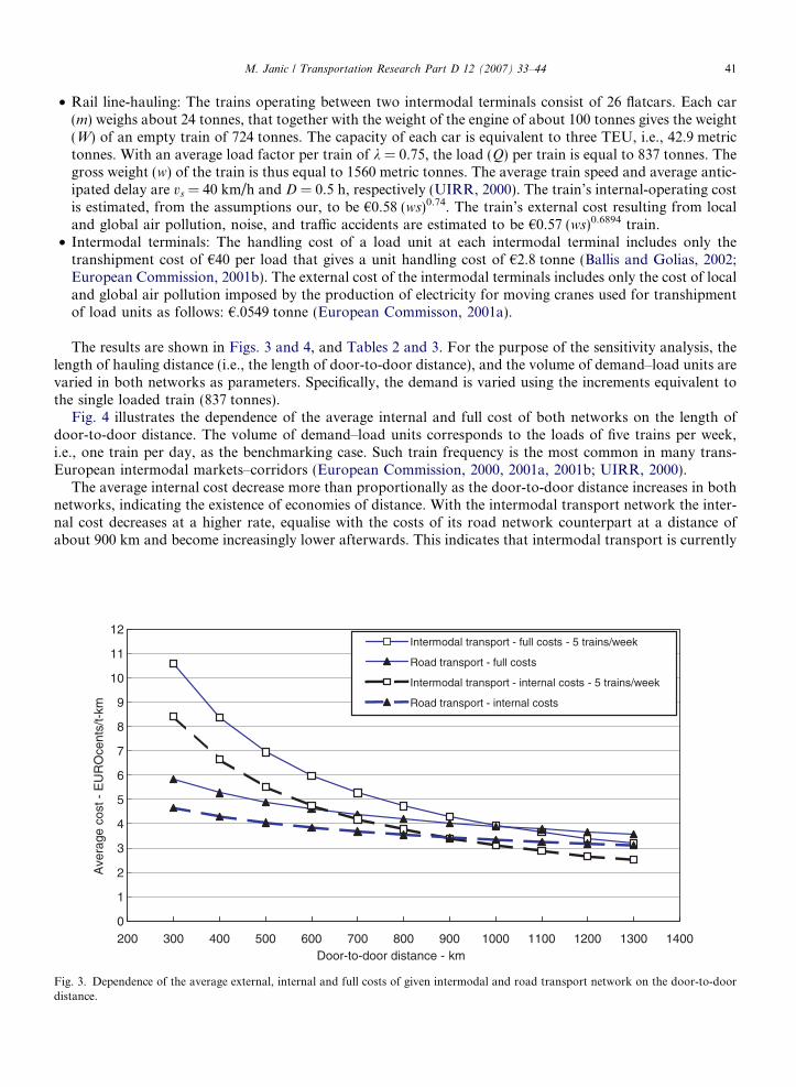
The results are shown in Figs. 3 and 4, and Tables 2 and 3. For the purpose of the sensitivity analysis, thelength of hauling distance (i.e., the length of door-to-door distance), and the volume of demand–load units arevaried in both networks as parameters. Specifically, the demand is varied using the increments equivalent tothe single loaded train (837 tonnes).

Fig. 4 illustrates the dependence of the average internal and full cost of both networks on the length ofdoor-to-door distance. The volume of demand–load units corresponds to the loads of five trains per week,i.e., one train per day, as the benchmarking case. Such train frequency is the most common in many trans-European intermodal markets–corridors (European Commission, 2000, 2001a, 2001b; UIRR, 2000).

The average internal cost decrease more than proportionally as the door-to-door distance increases in bothnetworks, indicating the existence of economies of distance. With the intermodal transport network the inter-nal cost decreases at a higher rate, equalise with the costs of its road network counterpart at a distance ofabout 900 km and become increasingly lower afterwards. This indicates that intermodal transport is currently

0

1

2

3

4

5

6

7

8

9

10

11

12

200 300 400 500 600 700 800 900 1000 1100 1200 1300 1400Door-to-door distance - km

Ave

rage

cos

t - E

UR

Oce

nts/

t-km

Intermodal transport - full costs - 5 trains/week

Road transport - full costs

Intermodal transport - internal costs - 5 trains/week

Road transport - internal costs

Fig. 3. Dependence of the average external, internal and full costs of given intermodal and road transport network on the door-to-doordistance.

0

1

2

3

4

5

6

7

8

9

10

11

12

200 300 400 500 600 700 800 900 1000 1100 1200 1300 1400

Door-to-door distance - km

Ave

rage

full

cost

- E

UR

Oce

nts/

t-km

Intermodal transport - 5 trains/weekIntermodal transport - 10 trains/weekIntermodal transport - 20 trains/weekIntermodal transport - 25 trains/weekRoad transport

vs = 40 km/h; d = 50 km; u = 35 km/h

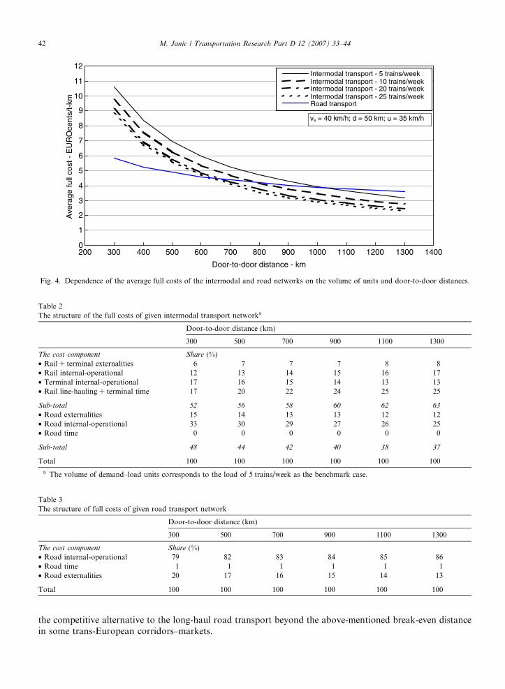
Fig. 4. Dependence of the average full costs of the intermodal and road networks on the volume of units and door-to-door distances.

Table 2The structure of the full costs of given intermodal transport networka

Door-to-door distance (km)

300 500 700 900 1100 1300

The cost component Share (%)• Rail + terminal externalities 6 7 7 7 8 8• Rail internal-operational 12 13 14 15 16 17• Terminal internal-operational 17 16 15 14 13 13• Rail line-hauling + terminal time 17 20 22 24 25 25

Sub-total 52 56 58 60 62 63

• Road externalities 15 14 13 13 12 12• Road internal-operational 33 30 29 27 26 25• Road time 0 0 0 0 0 0

Sub-total 48 44 42 40 38 37

Total 100 100 100 100 100 100

a The volume of demand–load units corresponds to the load of 5 trains/week as the benchmark case.

Table 3The structure of full costs of given road transport network

Door-to-door distance (km)

300 500 700 900 1100 1300

The cost component Share (%)• Road internal-operational 79 82 83 84 85 86• Road time 1 1 1 1 1 1• Road externalities 20 17 16 15 14 13

Total 100 100 100 100 100 100


the competitive alternative to the long-haul road transport beyond the above-mentioned break-even distancein some trans-European corridors–markets.


The relationship between the average internal costs of both networks may partially explain the current splitbetween the two modes in Europe. The operational cost of road transport is lower than the operational cost ofthe intermodal transport network over short, medium and even some long-distances markets, which, in com-bination with other market and regulatory factors leads to lower prices. This attract more of voluminous andprice sensitive commodities over such distances (about 90% up to 600 km).

For both networks, the sum of their internal and external costs also decreases more than proportionally asdoor-to-door distances increase. The rate of decrease is again higher in the intermodal transport network sug-gesting a break-even distance of about 1050 km. This is longer than for the operational costs. Since the volumeof demand around these distances is generally low, basing prices on the higher full costs may affect the alreadylow, although still price-sensitive, demand thus making conditions under which intermodal transport can gaina higher market shares even more complex. This raises questions about the efficiency of EU policies thatexpects internalising externalities to strengthen the market position of intermodal transport. Table 2 showsthe structure of the full costs of the intermodal transport network.

As the door-to-door distance increases, the share of the rail/terminal-related external costs increase and theshare of the road-related external costs decrease. The share of the road external costs is about twice that of therail-terminal related external costs. Consequently, the road operational steps at both ends of the intermodalnetwork contribute considerably to its external costs (about 40–50%).

In the absolute terms, the relatively constant shares of the rail and terminal internal costs are comparable tothe shares of road internal costs decreasing with increasing door-to-door distance. The shares of the time costsincrease in the rail-terminal case and appear negligible in both road operational steps. Consequently, increas-ing the door-to-door distance by about 1000 km (i.e., from 300 to 1300 km), increases the shares of the mainmode generally from 52% to 67% and decreases the share of the road mode from 48% to 37% (Table 3).

Increasing the door-to-door distance increases the share of internal costs from about 80%–86%, the share ofthe external costs decreases from 20% to 13%, while the share of time costs remains almost negligible.

Fig. 4 shows the influence on the average full costs of changing the volume of units and door-to-door distancein both networks. These costs of the road transport network are constant and those of the intermodal transportnetwork decrease as the volume of units increases. This diminishing of full costs reduces the break-even distancefor the intermodal network. For example, if demand increases from 5 trains a week to 10, the break-even distancewill shorten from about 1050 km to 800 km. If the demand increase is from 10 to 20 trains a week, the break-evendistance will decrease further to 650 km. Consequently, intermodal transport could enhance its competitivenessby increasing service frequencies of the main mode on the shorter distance services.

5. Conclusions

The paper developed a model for calculating the full costs of a given intermodal and road freight transportnetworks. The model is applied to simplified configurations of intermodal rail-truck and equivalent roadtransport networks in Europe. The results show that the full costs of both networks decrease more than pro-portionally as door-to-door distance increases; suggesting economies of distance. For the intermodal transportnetwork, the average full costs decrease at a decreasing rate as the quantity of loads rises indicating economiesof scale; in the road transport network they are constant.

Full and the internal costs decrease more rapidly with increasing distance in the intermodal case rather thanin the road transport network. Consequently, the costs of both networks equalised at a break-even distance –shorter for the internal measure and longer for full costs. Since the full costs of intermodal transport decreaseand the those of road transport remain constant as the volume of loads increases, the break-even distanceshortens at a decreasing rate.

Despite caveats inevitable in such estimations, the results offer some insight into EU policies aimed at inter-nalising transport externalities. If the full costs are to be used as the main bais for pricing, the break-even dis-tance will increase for intermodal transport and thus push the it to compete in longer distance markets, withincreasingly diminishing demand. However, intermodal transport can neutralise the effects of the higher pricesassociated with internalising by increasing the service frequencies in medium-distance markets (around 600–900 km) to meet the large demand there.


References

Ballis, A., Golias, J., 2002. Comparative evaluation of existing and innovative rail–road freight transport terminals. TransportationResearch A 36A, 593–611.

Bontekoning, Y., Macharis, C., Trip, J.J., 2004. Is a new applied transportation field emerging? – A review of intermodal rail–truck freighttransport literature. Transportation Research A 38A, 1–34.

Daganzo, C.F., 1999. Logistics System Analysis, third ed. Springer, Berlin.European Commisson 1999. The Common Transport Policy – Sustainable Mobility: Perspectives for the Future, European Commission,

Economic and Social Committee and Committee of the Regions, Directorate General DG VII, <http://europa.eu.int/en/comm/dg07/tif/>.

European Commisson 2000. The Way to Sustainable Mobility: Cutting the External Cost of Transport, Brochure of the EuropeanCommission, Brussels.

European Commisson 2001a. Real Cost Reduction of Door-to-door Intermodal Transport – RECORDIT, European Commissions,Directorate General DG VII, RTD 5th Framework Programme, Brussels, Belgium.

European Commisson 2001b. Improvement of Pre- and End- Haulage – IMPREND, European Commissions, Directorate General DGVII, RTD 4th Framework Programme, Brussels.

European Commisson 2002. EU Intermodal Transport: Key Statistical Data 1992–1999, European Commissions, Office for OfficialPublications of European Communities, Luxembourg.

European Conference of Ministers of Transport 1998. Report on the Current State of Combined Transport in Europe, EuropeanConference of Ministers of Transport, Paris.

Janic, M., Reggiani, A., Spicciareli, T., 1999. The European Freight Transport System: Theoretical Background of the New GenerationBundling Networks. In: Proceedings of the 8th WCTR – World Conference on Transport Research, vol. 1, Transport Modes andSystems, Antwerp.

Levison, D., Gillen, D., Kanafani, A., Mathieu, J.M., 1996. The Full Cost of Intercity Transportation – A Comparison of High-SpeedRail, Air and Highway Transportation in California, Institute of Transportation, University of California, Berkeley, Research Report,UCB-ITS-RR-96-3.

Morlok, E.K., Spasovic, L.N., Nozick, L.K., Sammon, J., 1995. Improving productivity in intermodal rail–truck transportation. In:Harker, P.T. (Ed.), The Service Productivity and Service Challenge. Kluwer, Amsterdam.

UIRR, 2000. Developing a Quality Strategy for Combined Transport, International Union of Combined Rail–Road TransportCompanies, Final Report, PACT Programme, Brussels.

http://europa.eu.int/en/comm/dg07/tif/

http://europa.eu.int/en/comm/dg07/tif/

modelling the full costs of an intermodal and road freight transport network

Documents