Modelling Dependence with Copulasand Applications to Risk Management

Paul Embrechts, Filip Lindskog∗ and Alexander McNeil∗∗

Department of MathematicsETHZ

CH-8092 ZurichSwitzerland

www.math.ethz.ch/finance

September 10, 2001

∗Research of the second author was supported by Credit Suisse Group, Swiss Re and UBS AG throughRiskLab, Switzerland. ∗∗The third author acknowledges financial support from Swiss Re.

i

Contents

1 Introduction 1

2 Copulas 22.1 Mathematical Introduction . . . . . . . . . . . . . . . . . . . . . . . . . . 22.2 Sklar’s Theorem . . . . . . . . . . . . . . . . . . . . . . . . . . . . . . . . 42.3 The Frechet–Hoeffding Bounds for Joint Distribution Functions . . . . . . 42.4 Copulas and Random Variables . . . . . . . . . . . . . . . . . . . . . . . . 6

3 Dependence Concepts 93.1 Linear Correlation . . . . . . . . . . . . . . . . . . . . . . . . . . . . . . . 93.2 Perfect Dependence . . . . . . . . . . . . . . . . . . . . . . . . . . . . . . . 103.3 Concordance . . . . . . . . . . . . . . . . . . . . . . . . . . . . . . . . . . 113.4 Kendall’s tau and Spearman’s rho . . . . . . . . . . . . . . . . . . . . . . 133.5 Tail Dependence . . . . . . . . . . . . . . . . . . . . . . . . . . . . . . . . 15

4 Marshall-Olkin Copulas 174.1 Bivariate Marshall-Olkin Copulas . . . . . . . . . . . . . . . . . . . . . . . 184.2 A Multivariate Extension . . . . . . . . . . . . . . . . . . . . . . . . . . . 204.3 A Useful Modelling Framework . . . . . . . . . . . . . . . . . . . . . . . . 21

5 Elliptical Copulas 225.1 Elliptical Distributions . . . . . . . . . . . . . . . . . . . . . . . . . . . . . 225.2 Gaussian Copulas . . . . . . . . . . . . . . . . . . . . . . . . . . . . . . . . 255.3 t-copulas . . . . . . . . . . . . . . . . . . . . . . . . . . . . . . . . . . . . . 26

6 Archimedean Copulas 306.1 Definitions . . . . . . . . . . . . . . . . . . . . . . . . . . . . . . . . . . . . 316.2 Properties . . . . . . . . . . . . . . . . . . . . . . . . . . . . . . . . . . . . 326.3 Kendall’s tau Revisited . . . . . . . . . . . . . . . . . . . . . . . . . . . . 346.4 Tail Dependence Revisited . . . . . . . . . . . . . . . . . . . . . . . . . . . 356.5 Multivariate Archimedean Copulas . . . . . . . . . . . . . . . . . . . . . . 37

7 Modelling Extremal Events in Practice 407.1 Insurance Risk . . . . . . . . . . . . . . . . . . . . . . . . . . . . . . . . . 407.2 Market Risk . . . . . . . . . . . . . . . . . . . . . . . . . . . . . . . . . . . 41

ii

1 Introduction

Integrated Risk Management (IRM) is concerned with the quantitative description ofrisks to a financial business. Whereas the qualitative aspects of IRM are extremely im-portant, in the present contribution we only concentrate on the quantitative ones. Sincethe emergence of Value-at-Risk (VaR) in the early nineties and its various generalisationsand refinements more recently, regulators and banking and insurance professionals havebuild up a huge system aimed at making the global financial system safer. Whereas thesteps taken no doubt have been very important towards increasing the overall risk aware-ness, continuously questions have been asked concerning the quality of the safeguards asconstructed.

All quantitative models are based on assumptions vis-a-vis the markets on whichthey are to be applied. Standard hedging techniques require a high level of liquidityof the underlying instruments, prices quoted for many financial products are often basedon “normal” conditions. The latter may be interpreted in a more economic sense, ormore specifically referring to the distributional (i.e. normal, Gaussian) behaviour of someunderlying data. Especially for IRM, deviations from the “normal” would constitute aprime source of investigation. Hence the classical literature is full of deviations from theso-called random walk (Brownian motion) model and heavy tails appear prominently. Thelatter has for instance resulted in the firm establishment of Extreme Value Theory (EVT)as a standard tool within IRM. Within market risk management, the so-called stylised factsof econometrics summarise this situation: market data returns tend to be uncorrelated,but dependent, they are heavy tailed, extremes appear in clusters and volatility is random.

Our contribution aims at providing tools for going one step further: what would bethe stylised facts of dependence in financial data? Is there a way of understanding so-called normal (i.e. Gaussian) dependence and how can we construct models which allowto go beyond normal dependence? Other problems we would like to understand betterare spillover, the behaviour of correlations under extreme market movements, the prosand contras of linear correlation as a measure of dependence, the construction of riskmeasures for functions of dependent risks. One example concerning the latter is thefollowing: suppose we have two VaR numbers corresponding to two different lines ofbusiness. In order to cover the joint position, can we just add the VaR? Under whichconditions is this always the upper bound? What can go wrong if these conditions arenot fulfilled? A further type of risk where dependence play a crucial role is credit risk:how to define, stress test and model default correlation. The present paper is not solvingthe above problem, it presents however tools which are crucial towards the constructionof solutions.

The notion we concentrate on is that of copula, well known for some time withinthe statistics literature. The word copula first appeared in the statistics literature 1959,Sklar (1959), although similar ideas and results can be traced back to Hoeffding (1940).Copulas allow us to construct models which go beyond the standard ones at the level ofdependence. They yield an ideal tool to stress test a wide variety of portfolios and productsin insurance and finance for extreme moves in correlation and more general measures ofdependence. As such, they gradually are becoming an extra, but crucial, element of bestpractice IRM. After Section 2 in which we define the concept of copula in full generality,we turn in Section 3 to an overview of the most important notions of dependence used inIRM. Section 4, 5 and 6 introduces the most important families of copulas, their propertiesboth methodological as well as with respect to simulation. Throughout these sections, we

1

stress the importance of the techniques introduced within an IRM framework. Finally inSection 7 we discuss some specific examples.

We would like to stress that the present paper only gives a first introduction aimedat bringing together from the extensive copula world those results which are immediatelyusable in IRM. Topics not included are statistical estimation of copulas and the modellingof dependence, through copulas, in a dynamic environment. As such, the topics listedcorrespond to a one-period point of view. Various extensions are possible; the interestedreader is referred to the bibliography for further reading.

2 Copulas

The standard “operational” definition of a copula is a multivariate distribution functiondefined on the unit cube [0, 1]n, with uniformly distributed marginals. This definitionis very natural if one considers how a copula is derived from a continuous multivariatedistribution function; indeed in this case the copula is simply the original multivariatedistribution function with transformed univariate margins. This definition however maskssome of the problems one faces when constructing copulas using other techniques, i.e. itdoes not say what is meant by a multivariate distribution function. For that reason, westart with a slightly more abstract definition, returning to the “operational” one later.Below, we follow Nelsen (1999) in concentrating on general multivariate distributions atfirst and then studying the special properties of the copula subset.

Throughout this paper, for a function H, we denote by DomH and RanH the domainand range respectively of H. Furthermore, a function f will be called increasing wheneverx ≤ y implies that f(x) ≤ f(y). We may also refer to this as f is nondecreasing. Astatement about points of a set S ⊂ R

n, where S is typically the real line or the unit cube[0, 1]n, is said to hold almost everywhere if the set of points of S where the statement failsto hold has Lebesgue measure zero.

2.1 Mathematical Introduction

Definition 2.1. Let S1, . . . , Sn be nonempty subsets of R, where R denotes the extendedreal line [−∞,∞]. Let H be a real function of n variables such that DomH = S1×· · ·×Sn

and for a ≤ b (ak ≤ bk for all k) let B = [a,b] (= [a1, b1] × · · · × [an, bn]) be an n-boxwhose vertices are in DomH. Then the H-volume of B is given by

VH(B) =∑

sgn(c)H(c),

where the sum is taken over all vertices c of B, and sgn(c) is given by

sgn(c) ={

1, if ck = ak for an even number of k’s,−1, if ck = ak for an odd number of k’s.

�

Equivalently, the H-volume of an n-box B = [a,b] is the nth order difference of H onB

VH(B) = 4baH(t) = 4bn

an. . .4b1

a1H(t),

where the n first order differences are defined as

4bkakH(t) = H(t1, . . . , tk−1, bk, tk+1, . . . , tn)−H(t1, . . . , tk−1, ak, tk+1, . . . , tn).

2

Definition 2.2. A real function H of n variables is n-increasing if VH(B) ≥ 0 for alln-boxes B whose vertices lie in DomH. �

Suppose that the domain of a real function H of n variables is given by DomH =S1 × · · · × Sn where each Sk has a smallest element ak. We say that H is grounded ifH(t) = 0 for all t in DomH such that tk = ak for at least one k. If each Sk is nonempty andhas a greatest element bk, then H has margins, and the one-dimensional margins of H arethe functions Hk with DomHk = Sk and with Hk(x) = H(b1, . . . , bk−1, x, bk+1, . . . , bn) forall x in Sk. Higher-dimensional margins are defined in an obvious way. One-dimensionalmargins are just called margins.

Lemma 2.1. Let S1, . . . , Sn be nonempty subsets of R, and let H be a grounded n-increasing function with domain S1×· · ·×Sn. Then H is increasing in each argument, i.e.,if (t1, . . . , tk−1, x, tk+1, . . . , tn) and (t1, . . . , tk−1, y, tk+1, . . . , tn) are in DomH and x ≤ y,then H(t1, . . . , tk−1, x, tk+1, . . . , tn) ≤ H(t1, . . . , tk−1, y, tk+1, . . . , tn).

Lemma 2.2. Let S1, . . . , Sn be nonempty subsets of R, and let H be a grounded n-increasing function with margins and domain S1×· · ·×Sn. Then, if x = (x1, . . . , xn) andy = (y1, . . . , yn) are any points in S1 × · · · × Sn,∣∣H(x)−H(y)

∣∣ ≤ n∑k=1

∣∣Hk(xk)−Hk(yk)∣∣.

For the proof, see Schweizer and Sklar (1983).

Definition 2.3. An n-dimensional distribution function is a function H with domain Rn

such that H is grounded, n-increasing and H(∞, . . . ,∞) = 1. �It follows from Lemma 2.1 that the margins of an n-dimensional distribution function

are distribution functions, which we denote F1, . . . , Fn.

Definition 2.4. An n-dimensional copula is a function C with domain [0, 1]n such that1. C is grounded and n-increasing.2. C has margins Ck, k = 1, 2, . . . , n, which satisfy Ck(u) = u for all u in [0, 1].

�Note that for any n-copula C, n ≥ 3, each k-dimensional margin of C is a k-copula.

Equivalently, an n-copula is a function C from [0, 1]n to [0, 1] with the following properties:

1. For every u in [0, 1]n, C(u) = 0 if at least one coordinate of u is 0, and C(u) = uk

if all coordinates of u equal 1 except uk.2. For every a and b in [0, 1]n such that ai ≤ bi for all i, VC([a,b]) ≥ 0.

Since copulas are joint distribution functions (on [0, 1]n), a copula C induces a prob-ability measure on [0, 1]n via

VC([0, u1]× · · · × [0, un]) = C(u1, . . . , un)

and a standard extension to arbitrary (not necessarily n-boxes) Borel subsets of [0, 1]n. Astandard result from measure theory says that there is a unique probability measure onthe Borel subsets of [0, 1]n which coincides with VC on the set of n-boxes of [0, 1]n. Thisprobability measure will also be denoted VC .

From Definition 2.4 it follows that a copula C is a distribution function on [0, 1]n withuniformly distributed (on [0, 1]) margins. The following theorem follows directly fromLemma 2.2.

3

Theorem 2.1. Let C be an n-copula. Then for every u and v in [0, 1]n,

∣∣C(v)−C(u)∣∣ ≤ n∑

k=1

∣∣vk − uk

∣∣.Hence C is uniformly continuous on [0, 1]n.

2.2 Sklar’s Theorem

The following theorem is known as Sklar’s Theorem. It is perhaps the most importantresult regarding copulas, and is used in essentially all applications of copulas.

Theorem 2.2. Let H be an n-dimensional distribution function with margins F1, . . . , Fn.Then there exists an n-copula C such that for all x in R

n,

H(x1, . . . , xn) = C(F1(x1), . . . , Fn(xn)). (2.1)

If F1, . . . , Fn are all continuous, then C is unique; otherwise C is uniquely determined onRanF1 × · · · × RanFn. Conversely, if C is an n-copula and F1, . . . , Fn are distributionfunctions, then the function H defined above is an n-dimensional distribution functionwith margins F1, . . . , Fn.

For the proof, see Sklar (1996).From Sklar’s Theorem we see that for continuous multivariate distribution functions,

the univariate margins and the multivariate dependence structure can be separated, andthe dependence structure can be represented by a copula.

Let F be a univariate distribution function. We define the generalized inverse of F asF−1(t) = inf{x ∈ R | F (x) ≥ t} for all t in [0, 1], using the convention inf ∅ = −∞.

Corollary 2.1. Let H be an n-dimensional distribution function with continuous marginsF1, . . . , Fn and copula C (where C satisfies (2.1)). Then for any u in [0, 1]n,

C(u1, . . . , un) = H(F−11 (u1), . . . , F−1

n (un)).

Without the continuity assumption, care has to be taken; see Nelsen (1999) or Marshall(1996).

Example 2.1. Let Φ denote the standard univariate normal distribution function and letΦn

R denote the standard multivariate normal distribution function with linear correlationmatrix R. Then

C(u1, . . . , un) = ΦnR(Φ−1(u1), . . . ,Φ−1(un))

is the Gaussian or normal n-copula. �

2.3 The Frechet–Hoeffding Bounds for Joint Distribution Functions

Consider the functions Mn, Πn and W n defined on [0, 1]n as follows:

Mn(u) = min(u1, . . . , un),Πn(u) = u1 . . . un,

W n(u) = max(u1 + · · · + un − n+ 1, 0).

The functions Mn and Πn are n-copulas for all n ≥ 2 whereas the function W n is not acopula for any n ≥ 3 as shown in the following example.

4

Example 2.2. Consider the n-cube [1/2, 1]n ⊂ [0, 1]n.

VW n([1/2, 1]n) = max(1 + · · ·+ 1− n+ 1, 0)− n max(1/2 + 1 + · · ·+ 1− n+ 1, 0)

+(n

2

)max(1/2 + 1/2 + 1 + · · ·+ 1− n+ 1, 0)

. . .

+ max(1/2 + · · · + 1/2− n+ 1, 0)= 1− n/2 + 0 + · · ·+ 0.

Hence W n is not a copula for n ≥ 3. �

The following theorem is called the Frechet–Hoeffding bounds inequality (Frechet (1957)).

Theorem 2.3. If C is any n-copula, then for every u in [0, 1]n,

W n(u) ≤ C(u) ≤Mn(u).

For more details, including geometrical interpretations, see Mikusinski, Sherwood, andTaylor (1992). Although the Frechet–Hoeffding lower bound W n is never a copula forn ≥ 3, it is the best possible lower bound in the following sense.

Theorem 2.4. For any n ≥ 3 and any u in [0, 1]n, there is an n-copula C (which dependson u) such that

C(u) = W n(u).

For the proof, see Nelsen (1999) p. 42.We denote by C the joint survival function for n random variables with joint distribu-

tion function C, i.e., if (U1, . . . , Un)T has distribution function C, then C(u1, . . . , un) =P{U1 > u1, . . . , Un > un}.Definition 2.5. If C1 and C2 are copulas, C1 is smaller than C2 (written C1 ≺ C2) if

C1(u) ≤ C2(u) and C1(u) ≤ C2(u),

for all u in [0, 1]n. �

Note that in the bivariate case,

C1(u1, u2) ≤ C2(u1, u2) ⇔ 1− u1 − u2 + C1(u1, u2) ≤ 1− u1 − u2 + C2(u1, u2)⇔ C1(u1, u2) ≤ C2(u1, u2).

The Frechet–Hoeffding lower bound W 2 is smaller than every 2-copula, and every n-copula is smaller than the Frechet–Hoeffding upper bound Mn. This partial ordering ofthe set of copulas is called a concordance ordering. It is a partial ordering since not everypair of copulas is comparable in this order. However many important parametric familiesof copulas are totally ordered. We call a one-parameter family

{Cθ

}positively ordered if

Cθ1 ≺ Cθ2 whenever θ1 ≤ θ2. Examples of such one-parameter families will be given later.

5

2.4 Copulas and Random Variables

Let X1, . . . ,Xn be random variables with continuous distribution functions F1, . . . , Fn,respectively, and joint distribution function H. Then (X1, . . . ,Xn)T has a unique copulaC, where C is given by (2.1). The standard copula representation of the distribution ofthe random vector (X1, . . . ,Xn)T then becomes:

H(x1, . . . , xn) = P{X1 ≤ x1, . . . ,Xn ≤ xn} = C(F1(x1), . . . , Fn(xn)).

The transformations Xi 7→ Fi(Xi) used in the above representation are usually referredto as the probability-integral transformations (to uniformity) and form a standard tool insimulation methodology.

Since X1, . . . ,Xn are independent if and only if H(x1, . . . , xn) = F1(x1) . . . Fn(xn) forall x1, . . . , xn in R, the following result follows from Theorem 2.2.

Theorem 2.5. Let (X1, . . . ,Xn)T be a vector of continuous random variables with copulaC, then X1, . . . ,Xn are independent if and only if C = Πn.

One nice property of copulas is that for strictly monotone transformations of therandom variables, copulas are either invariant, or change in certain simple ways. Notethat if the distribution function of a random variable X is continuous, and if α is a strictlymonotone function whose domain contains RanX, then the distribution function of therandom variable α(X) is also continuous.

Theorem 2.6. Let (X1, . . . ,Xn)T be a vector of continuous random variables with copulaC. If α1, . . . , αn are strictly increasing on RanX1, . . . ,RanXn, respectively, then also(α1(X1), . . . , αn(Xn))T has copula C.

Proof. Let F1, . . . , Fn denote the distribution functions of X1, . . . ,Xn and let G1, . . . , Gn

denote the distribution functions of α1(X1), . . . , αn(Xn), respectively. Let (X1, . . . ,Xn)T

have copula C, and let (α1(X1), . . . , αn(Xn))T have copula Cα. Since αk is strictly in-creasing for each k, Gk(x) = P{αk(Xk) ≤ x} = P{Xk ≤ α−1

k (x)} = Fk(α−1k (x)) for any x

in R, hence

Cα(G1(x1), . . . , Gn(xn)) = P{α1(X1) ≤ x1, . . . , αn(Xn) ≤ xn}= P{X1 ≤ α−1

1 (x1), . . . ,Xn ≤ α−1n (xn)}

= C(F1(α−11 (x1)), . . . , Fn(α−1

n (xn)))= C(G1(x1), . . . , Gn(xn)).

Since X1, . . . ,Xn are continuous, RanG1 = · · · = RanGn = [0, 1]. Hence it follows thatCα = C on [0, 1]n.

From Theorem 2.2 we know that the copula function C “separates” an n-dimensionaldistribution function from its univariate margins. The next theorem will show that thereis also a function, C, that separates an n-dimensional survival function from its univariatesurvival margins. Furthermore this function can be shown to be a copula, and this survivalcopula can rather easily be expressed in terms of C and its k-dimensional margins.

Theorem 2.7. Let (X1, . . . ,Xn)T be a vector of continuous random variables with copulaCX1,...,Xn. Let α1, . . . , αn be strictly monotone on RanX1, . . . ,RanXn, respectively, and

6

let (α1(X1), . . . , αn(Xn))T have copula Cα1(X1),...,αn(Xn). Furthermore let αk be strictlydecreasing for some k. Without loss of generality let k = 1. Then

Cα1(X1),...,αn(Xn)(u1, u2, . . . , un) = Cα2(X2),...,αn(Xn)(u2, . . . , un)− CX1,α2(X2),...,αn(Xn)(1− u1, u2, . . . , un).

Proof. Let X1, . . . ,Xn have distribution functions F1, . . . , Fn and let α1(X1), . . . , αn(Xn)have distribution functions G1, . . . , Gn. Then

Cα1(X1),α2(X2),...,αn(Xn)(G1(x1), . . . , Gn(xn))= P{α1(X1) ≤ x1, . . . , αn(Xn) ≤ xn}= P{X1 > α−1

1 (x1), α2(X2) ≤ x2, . . . , αn(Xn) ≤ xn}= P{α2(X2) ≤ x2, . . . , αn(Xn) ≤ xn}− P{X1 ≤ α−1

1 (x1), α2(X2) ≤ x2, . . . , αn(Xn) ≤ xn}= Cα2(X2),...,αn(Xn)(G2(x2), . . . , Gn(xn))

− CX1,α2(X2),...,αn(Xn)(F1(α−11 (x1)), G2(x2), . . . , Gn(xn))

= Cα2(X2),...,αn(Xn)(G2(x2), . . . , Gn(xn))− CX1,α2(X2),...,αn(Xn)(1−G1(x1), G2(x2), . . . , Gn(xn)),

from which the conclusion follows directly.

By using the two theorems above recursively it is clear that the copula Cα1(X1),...,αn(Xn)

can be expressed in terms of the copula CX1,...,Xn and its lower-dimensional margins. Thisis exemplified below.

Example 2.3. Consider the bivariate case.Let α1 be strictly decreasing and let α2 be strictly increasing. Then

Cα1(X1),α2(X2)(u1, u2) = u2 −CX1,α2(X2)(1− u1, u2)= u2 −CX1,X2(1− u1, u2).

Let α1 and α2 be strictly decreasing. Then

Cα1(X1),α2(X2)(u1, u2) = u2 − CX1,α2(X2)(1− u1, u2)= u2 −

(1− u1 − CX1,X2(1− u1, 1− u2)

)= u1 + u2 − 1 +CX1,X2(1− u1, 1− u2).

Here Cα1(X1),α2(X2) is the survival copula, C, of (X1,X2)T , i.e.,

H(x1, x2) = P{X1 > x1,X2 > x2} = C(F 1(x1), F 2(x2)).

�

Note also that the joint survival function of n U(0, 1) random variables whose jointdistribution function is the copula C is C(u1, . . . , un) = C(1− u1, . . . , 1− un).

The mixed kth order partial derivatives of a copula C, ∂kC(u)/∂u1 . . . ∂uk, exist foralmost all u in [0, 1]n. For such u, 0 ≤ ∂kC(u)/∂u1 . . . ∂uk ≤ 1. For details, see Nelsen(1999) p. 11. With this in mind, let

C(u1, . . . , un) = AC(u1, . . . , un) + SC(u1, . . . , un),

7

where

AC(u1, . . . , un) =∫ u1

0. . .

∫ un

0

∂n

∂s1 . . . ∂snC(s1, . . . , sn) ds1 . . . dsn,

SC(u1, . . . , un) = C(u1, . . . , un)−AC(u1, . . . , un).

Unlike multivariate distributions in general, the margins of a copula are continuous,hence a copula has no individual points u in [0, 1]n for which VC(u) > 0. If C =AC on [0, 1]n, then C is said to be absolutely continuous. In this case C has den-sity ∂n

∂u1...∂unC(u1, . . . , un). If C = SC on [0, 1]n, then C is said to be singular, and

∂n

∂u1...∂unC(u1, . . . , un) = 0 almost everywhere in [0, 1]n. The support of a copula is the

complement of the union of all open subsets A of [0, 1]n with VC(A) = 0. When C is sin-gular its support has Lebesgue measure zero and conversely. However a copula can havefull support without being absolutely continuous. Examples of such copulas are so-calledMarshall-Olkin copulas which are presented later.

Example 2.4. Consider the bivariate Frechet–Hoeffding upper bound M given byM(u, v) = min(u, v) on [0, 1]2. It follows that ∂2

∂u∂vM(u, v) = 0 everywhere on [0, 1]2

except on the main diagonal (which has Lebesgue measure zero), and VM (B) = 0 for ev-ery rectangle B in [0, 1]2 entirely above or below the main diagonal. Hence M is singular.�

One of the main aims of this paper is to present effective algorithms for random variategeneration from the various copula families studied. The properties of the specific copulafamily is often essential for the efficiency of the corresponding algorithm. We now presenta general algorithm for random variate generation from copulas. Note however that inmost cases it is not an efficient one to use.

Consider the general situation of random variate generation from the n-copula C. Let

Ck(u1, . . . , uk) = C(u1, . . . , uk, 1, . . . , 1), k = 2, . . . , n− 1,

denote k-dimensional margins of C, with C1(u1) = u1 and Cn(u1, . . . , un) = C(u1, . . . , un).Let U1, . . . , Un have joint distribution function C. Then the conditional distribution ofUk given the values of U1, . . . , Uk−1, is given by

Ck(uk | u1, . . . , uk−1) = P{Uk ≤ uk | U1 = u1, . . . , Uk−1 = uk−1}=

∂k−1Ck(u1, . . . , uk)∂u1 . . . ∂uk−1

/∂k−1Ck−1(u1, . . . , uk−1)∂u1 . . . ∂uk−1

,

given that the numerator and denominator exist and that the denominator is not zero.The following algorithm generates a random variate (u1, . . . , un)T from C. As usual, letU(0, 1) denote the uniform distribution on [0, 1].

Algorithm 2.1.

• Simulate a random variate u1 from U(0, 1).• Simulate a random variate u2 from C2(· | u1)....• Simulate a random variate un from Cn(· | u1, . . . , un−1).

�

8

This algorithm is in fact a particular case of what is called “the standard construction”.The correctness of the algorithm can be seen from the fact that for independent U(0, 1)random variables Q1, . . . , Qn,

(Q1, C−12 (Q2 | Q1), . . . , C−1

n (Qn | Q1, C−12 (Q2 | Q1), . . . ))T

has distribution function C. To simulate a value uk from Ck(· | u1, . . . , uk−1) in generalmeans simulating q from U(0, 1) from which uk = C−1

k (q | u1, . . . , uk−1) can be obtainedthrough the equation q = Ck(uk | u1, . . . , uk−1) by numerical rootfinding. When C−1

k (q |u1, . . . , uk−1) has a closed form (and hence there is no need for numerical rootfinding) thisalgorithm can be recommended.

Example 2.5. Let the copula C be given by C(u, v) = (u−θ + v−θ − 1)−1/θ, for θ > 0.Then

C2|1(v | u) =∂C

∂u(u, v) = −1

θ(u−θ + v−θ − 1)−1/θ−1(−θu−θ−1)

= (uθ)−1−θ

θ (u−θ + v−θ − 1)−1/θ−1 = (1 + uθ(v−θ − 1))−1−θ

θ .

Solving the equation q = C2|1(v | u) for v yields

C−12|1 (q | u) = v =

((q

−θ1+θ − 1)u−θ + 1

)−1/θ.

The following algorithm generates a random variate (u, v)T from the above copula C.

• Simulate two independent random variates u and q from U(0, 1).

• Set v = ((q−θ1+θ − 1)u−θ + 1)−1/θ.

�

3 Dependence Concepts

Copulas provide a natural way to study and measure dependence between random vari-ables. As a direct consequence of Theorem 2.6, copula properties are invariant understrictly increasing transformations of the underlying random variables. Linear correlation(or Pearson’s correlation) is most frequently used in practice as a measure of dependence.However, since linear correlation is not a copula-based measure of dependence, it can oftenbe quite misleading and should not be taken as the canonical dependence measure. Belowwe recall the basic properties of linear correlation, and then continue with some copulabased measures of dependence.

3.1 Linear Correlation

Definition 3.1. Let (X,Y )T be a vector of random variables with nonzero finite variances.The linear correlation coefficient for (X,Y )T is

ρ(X,Y ) =Cov(X,Y )√

Var(X)√

Var(Y ), (3.1)

where Cov(X,Y ) = E(XY ) − E(X)E(Y ) is the covariance of (X,Y )T , and Var(X) andVar(Y ) are the variances of X and Y . �

9

Linear correlation is a measure of linear dependence. In the case of perfect lineardependence, i.e., Y = aX + b almost surely for a ∈ R \ {0}, b ∈ R, we have |ρ(X,Y )| =1. More important is that the converse also holds. Otherwise, −1 < ρ(X,Y ) < 1.Furthermore linear correlation has the property that

ρ(αX + β, γY + δ) = sign(αγ)ρ(X,Y ),

for α, γ ∈ R \ {0}, β, δ ∈ R. Hence linear correlation is invariant under strictly increasinglinear transformations. Linear correlation is easily manipulated under linear operations.Let A,B be m× n matrices; a, b ∈ R

m and let X,Y be random n-vectors. Then

Cov(AX + a,BY + b) = ACov(X,Y)BT .

From this it follows that for α ∈ Rn,

Var(αT X) = αT Cov(X)α,

where Cov(X) := Cov(X,X). Hence the variance of a linear combination is fully deter-mined by pairwise covariances between the components, a property which is crucial inportfolio theory.

Linear correlation is a popular but also often misunderstood measure of dependence.The popularity of linear correlation stems from the ease with which it can be calculatedand it is a natural scalar measure of dependence in elliptical distributions (with well knownmembers such as the multivariate normal and the multivariate t-distribution). Howevermost random variables are not jointly elliptically distributed, and using linear correlationas a measure of dependence in such situations might prove very misleading. Even forjointly elliptically distributed random variables there are situations where using linearcorrelation, as defined by (3.1), does not make sense. We might choose to model somescenario using heavy-tailed distributions such as t2-distributions. In such cases the linearcorrelation coefficient is not even defined because of infinite second moments.

3.2 Perfect Dependence

For every n-copula C we know from the Frechet–Hoeffding inequality (Theorem 2.3) that

W n(u1, . . . , un) ≤ C(u1, . . . , un) ≤Mn(u1, . . . , un).

Furthermore, for n = 2 the upper and lower bounds are themselves copulas and wehave seen that W and M are the bivariate distributions functions of the random vectors(U, 1−U)T and (U,U)T , respectively, where U ∼ U(0, 1) (i.e. U is uniformly distributed on[0, 1]). In this case we say that W describes perfect negative dependence and M describesperfect positive dependence.

Theorem 3.1. Let (X,Y )T have one of the copulas W or M . Then there exist twomonotone functions α, β : R −→ R and a random variable Z so that

(X,Y ) =d (α(Z), β(Z)),

with α increasing and β decreasing in the former case (W ) and both α and β increasingin the latter case (M). The converse of this result is also true.

10

For a proof, see Embrechts, McNeil, and Straumann (1999). In a different form this resultwas already in Frechet (1951).

Definition 3.2. If (X,Y )T has the copula M then X and Y are said to be comonotonic;if it has the copula W they are said to be countermonotonic. �

Note that if any of F and G (the distribution functions of X and Y , respectively) havediscontinuities, so that the copula is not unique, then W and M are possible copulas. Inthe case of F and G being continuous, a stronger version of the result can be stated:

C = W ⇔ Y = T (X) a.s., T = G−1 ◦ (1− F ) decreasing,C = M ⇔ Y = T (X) a.s., T = G−1 ◦ F increasing.

Other characterizations of comonotonicity can be found in Denneberg (1994).

3.3 Concordance

Let (x, y)T and (x, y)T be two observations from a vector (X,Y )T of continuous randomvariables. Then (x, y)T and (x, y)T are said to be concordant if (x − x)(y − y) > 0, anddiscordant if (x− x)(y − y) < 0.

The following theorem can be found in Nelsen (1999) p. 127. Many of the results inthis section are direct consequences of this theorem.

Theorem 3.2. Let (X,Y )T and (X, Y )T be independent vectors of continuous randomvariables with joint distribution functions H and H, respectively, with common marginsF (of X and X) and G (of Y and Y ). Let C and C denote the copulas of (X,Y )T and(X, Y )T , respectively, so that H(x, y) = C(F (x), G(y)) and H(x, y) = C(F (x), G(y)). LetQ denote the difference between the probability of concordance and discordance of (X,Y )T

and (X, Y )T , i.e. let

Q = P{(X − X)(Y − Y ) > 0} − P{(X − X)(Y − Y ) < 0}.

ThenQ = Q(C, C) = 4

∫∫[0,1]2

C(u, v) dC(u, v) − 1.

Proof. Since the random variables are all continuous, P{(X−X)(Y −Y ) < 0} = 1−P{(X−X)(Y − Y ) > 0} and hence Q = 2P{(X − X)(Y − Y ) > 0}− 1. But P{(X − X)(Y − Y ) >0} = P{X > X, Y > Y } + P{X < X, Y < Y }, and these probabilities can be evaluatedby integrating over the distribution of one of the vectors (X,Y )T or (X, Y )T . Hence

P{X > X, Y > Y } = P{X < X, Y < Y }=

∫∫R2

P{X < x, Y < y}dC(F (x), G(y))

=∫∫R2

C(F (x), G(y)) dC(F (x), G(y)),

Employing the probability-integral transforms u = F (x) and v = G(y) then yields

P{X > X, Y > Y } =∫∫

[0,1]2C(u, v) dC(u, v).

11

Similarly,

P{X < X, Y < Y } =∫∫R2

P{X > x, Y > y}dC(F (x), G(y))

=∫∫R2

{1− F (x)−G(y) + C(F (x), G(y))}dC(F (x), G(y))

=∫∫

[0,1]2{1− u− v + C(u, v)}dC(u, v).

But since C is the joint distribution function of a vector (U, V )T of U(0, 1) random vari-ables, E(U) = E(V ) = 1/2, and hence

P{X < X, Y < Y } = 1− 12− 1

2+∫∫

[0,1]2C(u, v) dC(u, v) =

∫∫[0,1]2

C(u, v) dC(u, v).

ThusP{(X − X)(Y − Y ) > 0} = 2

∫∫[0,1]2

C(u, v) dC(u, v),

and the conclusion follows.

Corollary 3.1. Let C, C, and Q be as given in Theorem 3.2. Then

1. Q is symmetric in its arguments: Q(C, C) = Q(C, C).2. Q is nondecreasing in each argument: if C ≺ C ′, then Q(C, C) ≤ Q(C ′, C).

3. Copulas can be replaced by survival copulas in Q, i.e. Q(C, C) = Q(C, C).

The following definition can be found in Scarsini (1984).

Definition 3.3. A real valued measure κ of dependence between two continuous randomvariablesX and Y whose copula is C is a measure of concordance if it satisfies the followingproperties:

1. κ is defined for every pair X,Y of continuous random variables.2. −1 ≤ κX,Y ≤ 1, κX,X = 1 and κX,−X = −1.3. κX,Y = κY,X .4. If X and Y are independent, then κX,Y = κΠ = 0.5. κ−X,Y = κX,−Y = −κX,Y .6. If C and C are copulas such that C ≺ C, then κC ≤ κC .7. If {(Xn, Yn)} is a sequence of continuous random variables with copulas

Cn, and if {Cn} converges pointwise to C, then limn→∞ κCn = κC .

�

Let κ be a measure of concordance for continuous random variables X and Y . As aconsequence of Definition 3.3, if If Y is almost surely an increasing function of X, thenκX,Y = κM = 1, and if Y is almost surely a decreasing function of X, then κX,Y = κW =−1. Moreover, if α and β are almost surely strictly increasing functions on RanX andRanY respectively, then κα(X),β(Y ) = κX,Y .

12

3.4 Kendall’s tau and Spearman’s rho

In this section we discuss two important measures of dependence (concordance) knownas Kendall’s tau and Spearman’s rho. They provide the perhaps best alternatives to thelinear correlation coefficient as a measure of dependence for nonelliptical distributions, forwhich the linear correlation coefficient is inappropriate and often misleading. For moredetails about Kendall’s tau and Spearman’s rho and their estimators (sample versions)we refer to Kendall and Stuart (1979), Kruskal (1958), Lehmann (1975) and Caperaa andGenest (1993). For other interesting scalar measures of dependence see Schweizer andWolff (1981).

Definition 3.4. Kendall’s tau for the random vector (X,Y )T is defined as

τ(X,Y ) = P{(X − X)(Y − Y ) > 0} − P{(X − X)(Y − Y ) < 0},where (X, Y )T is an independent copy of (X,Y )T . �

Hence Kendall’s tau for (X,Y )T is simply the probability of concordance minus theprobability of discordance.

Theorem 3.3. Let (X,Y )T be a vector of continuous random variables with copula C.Then Kendall’s tau for (X,Y )T is given by

τ(X,Y ) = Q(C,C) = 4∫∫

[0,1]2C(u, v) dC(u, v) − 1.

Note that the integral above is the expected value of the random variable C(U, V ),where U, V ∼ U(0, 1) with joint distribution function C, i.e. τ(X,Y ) = 4E(C(U, V ))− 1.

Definition 3.5. Spearman’s rho for the random vector (X,Y )T is defined as

ρS(X,Y ) = 3(P{(X − X)(Y − Y ′) > 0} − P{(X − X)(Y − Y ′) < 0}),where (X,Y )T , (X, Y )T and (X ′, Y ′)T are independent copies. �

Note that X and Y ′ are independent. Using Theorem 3.2 and the first part of Corollary3.1 we obtain the following result.

Theorem 3.4. Let (X,Y )T be a vector of continuous random variables with copula C.Then Spearman’s rho for (X,Y )T is given by

ρS(X,Y ) = 3Q(C,Π) = 12∫∫

[0,1]2uv dC(u, v)− 3 = 12

∫∫[0,1]2

C(u, v) dudv − 3.

Hence, if X ∼ F and Y ∼ G, and we let U = F (X) and V = G(Y ), then

ρS(X,Y ) = 12∫∫

[0,1]2uv dC(u, v)− 3 = 12E(UV )− 3

=E(UV )− 1/4

1/12=

Cov(U, V )√Var(U)

√Var(V )

= ρ(F (X), G(Y )).

In the next theorem we will see that Kendall’s tau and Spearman’s rho are concordancemeasures according to Definition 3.3.

13

Theorem 3.5. If X and Y are continuous random variables whose copula is C, thenKendall’s tau and Spearman’s rho satisfy the properties in Definition 3.3 for a measure ofconcordance.

For a proof, see Nelsen (1999) p. 137.

Example 3.1. Kendall’s tau and Spearman’s rho for the random vector (X,Y )T areinvariant under strictly increasing componentwise transformations. This property doesnot hold for linear correlation. It is not difficult to construct examples, the followingconstruction is instructive in its own right. Let X and Y be standard exponential randomvariables with copula C, where C is a member of the Farlie-Gumbel-Morgenstern family,i.e. C is given by

C(u, v) = uv + θuv(1− u)(1 − v),for some θ in [−1, 1]. The joint distribution function H of X and Y is given by

H(x, y) = C(1− e−x, 1− e−y).

Let ρ denote the linear correlation coefficient. Then

ρ(X,Y ) =E(XY )− E(X)E(Y )√

Var(X)√

Var(Y )= E(XY )− 1,

where

E(XY ) =∫ ∞

0

∫ ∞

0xy dH(x, y)

=∫ ∞

0

∫ ∞

0xy((1 + θ)e−x−y − 2θe−2x−y − 2θe−x−2y + 4θe−2x−2y

)dxdy

= 1 +θ

4.

Hence ρ(X,Y ) = θ/4. But

ρ(1− e−X , 1− e−Y ) = ρS(X,Y )

= 12∫∫

[0,1]2C(u, v) dudv − 3

= 12∫∫

[0,1]2(uv + θuv(1− u)(1 − v)) dudv − 3

= 12(14

+θ

36)− 3

= θ/3.

Hence ρ(X,Y ) is not invariant under strictly increasing transformations of X and Y andtherefore linear correlation is not a measure of concordance. �

Although the properties listed under Definition 3.3 are useful, there are some additionalproperties that would make a measure of concordance even more useful. Recall that for arandom vector (X,Y )T with copula C,

C = M =⇒ τC = ρC = 1,C = W =⇒ τC = ρC = −1.

The following theorem states that the converse is also true.

14

Theorem 3.6. Let X and Y be continuous random variables with copula C, and let κdenote Kendall’s tau or Spearman’s rho. Then the following are true:

1. κ(X,Y ) = 1 ⇐⇒ C = M .2. κ(X,Y ) = −1 ⇐⇒ C = W .

For a proof, see Embrechts, McNeil, and Straumann (1999).From the definitions of Kendall’s tau and Spearman’s rho it follows that both are in-

creasing functions of the value of the copula under consideration. Thus they are increasingwith respect to the concordance ordering given in Definition 2.5. Moreover, for continuousrandom variables all values in the interval [−1, 1] can be obtained for Kendall’s tau orSpearman’s rho by a suitable choice of the underlying copula. This is however not thecase with linear correlation as is shown in the following example from Embrechts, McNeil,and Straumann (1999).

Example 3.2. Let X ∼ LN(0, 1) (Lognormal) and Y ∼ LN(0, σ2), σ > 0. Then ρmin =ρ(eZ , e−σZ) and ρmax = ρ(eZ , eσZ), where Z ∼ N (0, 1). ρmin and ρmax can be calculated,yielding:

ρmin =e−σ − 1√

e− 1√eσ2 − 1

, ρmax =eσ − 1√

e− 1√eσ2 − 1

,

from which follows that limσ→∞ ρmin = limσ→∞ ρmax = 0. Hence the linear correlationcoefficient can be almost zero, even if X and Y are comonotonic or countermonotonic. �

Kendall’s tau and Spearman’s rho are measures of dependence between two randomvariables. However the extension to higher dimensions is obvious, we simply write pairwisecorrelations in an n× n matrix in the same way as is done for linear correlation.

3.5 Tail Dependence

The concept of tail dependence relates to the amount of dependence in the upper-right-quadrant tail or lower-left-quadrant tail of a bivariate distribution. It is a concept thatis relevant for the study of dependence between extreme values. It turns out that taildependence between two continuous random variables X and Y is a copula property andhence the amount of tail dependence is invariant under strictly increasing transformationsof X and Y .

Definition 3.6. Let (X,Y )T be a vector of continuous random variables with marginaldistribution functions F and G. The coefficient of upper tail dependence of (X,Y )T is

limu↗1

P{Y > G−1(u)|X > F−1(u)} = λU

provided that the limit λU ∈ [0, 1] exists. If λU ∈ (0, 1], X and Y are said to be asymp-totically dependent in the upper tail; if λU = 0, X and Y are said to be asymptoticallyindependent in the upper tail. �Since P{Y > G−1(u) | X > F−1(u)} can be written as

1− P{X ≤ F−1(u)} − P{Y ≤ G−1(u)} + P{X ≤ F−1(u), Y ≤ G−1(u)}1− P{X ≤ F−1(u)} ,

an alternative and equivalent definition (for continuous random variables), from which itis seen that the concept of tail dependence is indeed a copula property, is the followingwhich can be found in Joe (1997), p. 33.

15

Definition 3.7. If a bivariate copula C is such that

limu↗1

(1− 2u+ C(u, u))/(1 − u) = λU

exists, then C has upper tail dependence if λU ∈ (0, 1], and upper tail independence ifλU = 0. �

Example 3.3. Consider the bivariate Gumbel family of copulas given by

Cθ(u, v) = exp(−[(− lnu)θ + (− ln v)θ]1/θ),

for θ ≥ 1. Then

1− 2u+ C(u, u)1− u

=1− 2u+ exp(21/θ lnu)

1− u=

1− 2u+ u21/θ

1− u,

and hence

limu↗1

(1− 2u+ C(u, u))/(1 − u) = 2− limu↗1

21/θu21/θ−1 = 2− 21/θ.

Thus for θ > 1, Cθ has upper tail dependence. �

For copulas without a simple closed form an alternative formula for λU is more useful.An example is given in the case of the Gaussian copula

CR(u, v) =∫ Φ−1(u)

−∞

∫ Φ−1(v)

−∞

12π√

1−R212

exp{−s2 − 2R12st+ t2

2(1 −R212)

}ds dt,

where −1 < R12 < 1 and Φ is the univariate standard normal distribution function.Consider a pair of U(0, 1) random variables (U, V ) with copula C. First note that P{V ≤v | U = u} = ∂C(u, v)/∂u and P{V > v | U = u} = 1− ∂C(u, v)/∂u, and similarly whenconditioning on V . Then

λU = limu↗1

C(u, u)/(1 − u)

= − limu↗1

dC(u, u)du

= − limu↗1

(−2 +∂

∂sC(s, t)

∣∣s=t=u

+∂

∂tC(s, t)

∣∣s=t=u

)

= limu↗1

(P{V > u | U = u}+ P{U > u | V = u}).

Furthermore, if C is an exchangeable copula, i.e. C(u, v) = C(v, u), then the expressionfor λU simplifies to

λU = 2 limu↗1

P{V > u | U = u}.

Example 3.4. Let (X,Y )T have the bivariate standard normal distribution functionwith linear correlation coefficient ρ. That is (X,Y )T ∼ C(Φ(x),Φ(y)), where C is amember of the Gaussian family given above with R12 = ρ. Since copulas in this familyare exchangeable,

λU = 2 limu↗1

P{V > u | U = u},

16

and because Φ is a distribution function with infinite right endpoint,

limu↗1

P{V > u | U = u} = limx→∞P{Φ−1(V ) > x | Φ−1(U) = x} = lim

x→∞P{X > x | Y = x}.

Using the well known fact that Y | X = x ∼ N (ρx, 1− ρ2) we obtain

λU = 2 limx→∞Φ((x− ρx)/

√1− ρ2) = 2 lim

x→∞Φ(x√

1− ρ/√

1 + ρ),

from which it follows that λU = 0 for R12 < 1. Hence the Gaussian copula C with ρ < 1does not have upper tail dependence. �

The concept of lower tail dependence can be defined in a similar way. If the limitlimu↘0C(u, u)/u = λL exists, then C has lower tail dependence if λL ∈ (0, 1], and lowertail independence if λL = 0. For copulas without a simple closed form an alternativeformula for λL is more useful. Consider a random vector (U, V )T with copula C. Then

λL = limu↘0

C(u, u)/u = limu↘0

dC(u, u)du

= limu↘0

(∂

∂sC(s, t)

∣∣s=t=u

+∂

∂tC(s, t)

∣∣s=t=u

)

= limu↘0

(P{V < u | U = u}+ P{U < u | V = u}).

Furthermore if C is an exchangeable copula, i.e. C(u, v) = C(v, u), then the expressionfor λL simplifies to

λL = 2 limu↘0

P{V < u | U = u}.

Recall that the survival copula of two random variables with copula C is given by

C(u, v) = u+ v − 1 + C(1− u, 1− v),

and the joint survival function for two U(0, 1) random variables whose joint distributionfunction is C is given by

C(u, v) = 1− u− v + C(u, v) = C(1− u, 1− v).

Hence it follows that

limu↗1

C(u, u)/(1 − u) = limu↗1

C(1− u, 1− u)/(1 − u) = limu↘0

C(u, u)/u,

so the coefficient of upper tail dependence of C is the coefficient of lower tail dependenceof C. Similarly the coefficient of lower tail dependence of C is the coefficient of upper taildependence of C.

4 Marshall-Olkin Copulas

In this section we discuss a class of copulas called Marshall-Olkin copulas. To be able toderive these copulas and present explicit expressions for rank correlation and tail depen-dence coefficients without tedious calculations, we begin with bivariate Marshall-Olkincopulas. We then continue with the general n-dimensional case and suggest applicationsof Marshall-Olkin copulas to the modelling of dependent risks. For further details aboutMarshall-Olkin distributions we refer to Marshall and Olkin (1967). Similar ideas arecontained in Muliere and Scarsini (1987).

17

4.1 Bivariate Marshall-Olkin Copulas

Consider a two-component system where the components are subject to shocks, which arefatal to one or both components. Let X1 and X2 denote the lifetimes of the two compo-nents. Furthermore assume that the shocks follow three independent Poisson processeswith parameters λ1, λ2, λ12 ≥ 0, where the index indicates whether the shocks effect onlycomponent 1, only component 2 or both. Then the times Z1, Z2 and Z12 of occurrenceof these shocks are independent exponential random variables with parameters λ1, λ2 andλ12 respectively. Hence

H(x1, x2) = P{X1 > x1,X2 > x2} = P{Z1 > x1}P{Z2 > x2}P{Z12 > max(x1, x2)}.The univariate survival functions for X1 and X2 are F 1(x1) = exp(−(λ1 + λ12)x1) andF 2(x2) = exp(−(λ2 + λ12)x2). Furthermore, since max(x1, x2) = x1 + x2 −min(x1, x2),

H(x1, x2) = exp(−(λ1 + λ12)x1 − (λ2 + λ12)x2 + λ12 min(x1, x2))= F 1(x1)F 2(x2)min(exp(λ12x1), exp(λ12x2)).

Let α1 = λ12/(λ1 + λ12) and α2 = λ12/(λ2 + λ12). Then exp(λ12x1) = F 1(x1)−α1 andexp(λ12x2) = F 2(x2)−α2 , and hence the survival copula of (X1,X2)T is given by

C(u1, u2) = u1u2 min(u−α11 , u−α2

2 ) = min(u1−α11 u2, u1u

1−α22 ).

This construction leads to a copula family given by

Cα1,α2(u1, u2) = min(u1−α11 u2, u1u

1−α22 ) =

{u1−α1

1 u2, uα11 ≥ uα2

2 ,

u1u1−α22 , uα1

1 ≤ uα22 .

This family is known as the Marshall-Olkin family. Marshall-Olkin copulas have both anabsolutely continuous and a singular component. Since

∂2

∂u1∂u2Cα1,α2(u1, u2) =

{u−α1

1 , uα11 > uα2

2 ,

u−α22 , uα1

1 < uα22 ,

the mass of the singular component is concentrated on the curve uα11 = uα2

2 in [0, 1]2 asseen in Figure 4.1.

Kendall’s tau and Spearman’s rho are quite easily evaluated for this copula family.For Spearman’s rho, applying Theorem 3.4 yields:

ρS(Cα1,α2) = 12∫∫

[0,1]2Cα1,α2(u, v) dudv − 3

= 12∫ 1

0

(∫ uα1/α2

0u1−α1v dv +

∫ 1

uα1/α2

uv1−α2 dv

)du− 3

=3α1α2

2α1 + 2α2 − α1α2.

To evaluate Kendall’s tau we use the following theorem, a proof of which is found inNelsen (1999) p. 131.

Theorem 4.1. Let C be a copula such that the product(∂C/∂u

)(∂C/∂v

)is integrable

on [0, 1]2. Then∫∫[0,1]2

C(u, v) dC(u, v) =12−∫∫

[0,1]2

∂

∂uC(u, v)

∂

∂uC(u, v) dudv.

18

•

•

•

•

•

••

•

•

•

•

•

•

• •

•

•

•

•

•

•

•

•

•

•

•

•

•

•

•

•

•

•

•

•

•

•

•

•••

•

•

•

••

•

•

•

•

•

•

•

•

•

•

•

•

•

•

•

•

•

•

•

•

•

•

•

•

••

•

•

•

•

•

•

•

••

•

•

•

••

•

•

••

•

•

•

•

•

•

•

•

•

•

•

• •

•

•

•

•

•

•

•

••

•

•

•

•

•

•

•

•

•

•

•

•

•

•

•

•

•

•

••

••

•

•

•

•

•

•

•

•

•

•

•

•

•

•

•

•

•

••

•

•

•

•

•

•

•

•

•• •

•

•

•

•

•

•

•

•

•

•

•

•

•

•

•

•

•

•

•

•

• •

•

•

•

•

•

• •

•

•

•

•

•

•

•

•

•

•

•

•

•

•

•

•

•

•

• •

••

•

•

••

•

•

•

•

•

•

•

•

•

•

•

•

•

•

•

•

•

•

•

•

•

•

•

••

•

•

•

•

•

•

•

•

•

•

•

•

•

•

•

••

• •

•

•

•

•

•

•

•

•

•

•

•

•

•

•

•

•

•

•

•

•

•

•

•

•

••

•

•

•

•

•

•

•

•

•

•

•

•

•

•

•

•

•

•

•

•

•

•

•

•

•

•

•

•

•

•

•

•

•

•

•

•

•

•

•

•

•

•

•

•

•

•

•

•

•

•

•

•

•

• •

••

•

•

•

•

•

•

•

•

•

•

•

•

•

•

•

•

•

•

•

•

••

•

•

•

•

•••

•

•

•

•

•

••

•

•

••

• •

•

•

•

•

•

•

•

•

•

•

•

•

•

••

•

•

••

•

•

•

•

•

•

•

•

•

•

•

•

•

•

•

•

••

•

•

•

•

•

••

•

•

•

•

•

•

•

•

•

•

•

•

•

•

•

•

•

•

•

•

•

•

•

•

•

•

•

•

•

•

•

••

••

•

•

•

•

•

•

•

•

•

•

•

•

•

•

•

•

•

•

••

•

•

•

•

•

•

•

•

•

•

•

•

•

•

•

•

•

•

••

•

•

•

• •

•

•

•

•

•

••

•

•

•

•

•

•

•

•

•

• ••

•

•

••

•

•

•

•

•

••

•

•

•

•

•

•

•

•

•

•

•

•

• •

•

•

•

•

•

•

••

•

•

•

•

•

•

•

•

•

•

••

••

•

••

•

•

•

•

•

•

•

•

•

•

•

•

•

•

•

•

•

••

•

•

•

••

•

•

•

••

•

•

••

•

•

•

•

•

•

•

•

•

••

•

•

•

•

•

•

••

•

•

•

•

•

•

•

••

•

•

•

•

•

•

•

•

• •

•

•

•

••

•

•

•

•

•

•

•

•

•

•

•

•

•

•

•

•

•

•

•

•

•

•

•

•

•

•

•

•

•

•

•

•

•

•

•

•

•

•

•

••

••

•

••

•

•

•

•

•

•

•

•

•

•

•

••

•

•

•

•

•

•

•

•

•

•

•

•

•

•

•

•

•

•

•

•

•

••

•

•

••

•

•

•

•

•

•

•

•

•

•

•

•

•

•

•

•

•

•

•

•

•

•

•

•

•

•

•

•

•

•

••

•

••

•

•

•

•

•

•

••

•

•

•

•

•

•

•

•

•

••

•

•

•

•

•

•

••

•

•

•

•

•

••

•

•

•

•

•

••

•

•

•

• •

••

•

•

••

•

•

•

•

•

•

•

•

•

•

••

•

•

•

•

•

•

•

•

•

•

•

•

•

•

• •

•

•

•

•

•

•

•

•

•

•

•

•

• •

•

•

•

•

•

•

•

••

•

••

•

•

•

•

•

•••

•

• •

•

•

•

•

•

•

•

• •

•

•

•

•

•

•

•

••

•

•

•

•

•

•

•

•

•

•

•

•

•

•

•

••

•

••

•

•

• ••

•

•

•

•

•

•

•

•

•

•

•

•

•

•

•

••

••

•

•

•

•

•

•

•

•

•

•

• •

•

•

•

•

••

•

•

•

•

•

•

•

•

•

•

•

•

•

•

••

• •

•

•

•

•

•

•

•

Marshall-Olkin

X

Y

0.0 0.2 0.4 0.6 0.8 1.0

0.0

0.2

0.4

0.6

0.8

1.0

Figure 4.1: A simulation from the Marshall-Olkin copula with λ1 = 1.1, λ2 = 0.2 andλ12 = 0.6.

Using Theorems 3.3 and 4.1 we obtain

τ(Cα1,α2) = 4∫∫

[0,1]2Cα1,α2(u, v) dCα1,α2(u, v) − 1

= 4

(12−∫∫

[0,1]2

∂

∂uCα1,α2(u, v)

∂

∂uCα1,α2(u, v) dudv

)− 1

=α1α2

α1 + α2 − α1α2.

Thus, all values in the interval [0, 1] can be obtained for ρS(Cα1,α2) and τ(Cα1,α2). TheMarshall-Olkin copulas have upper tail dependence. Without loss of generality assumethat α1 > α2, then

limu↗1

C(u, u)1− u

= limu↗1

1− 2u+ u2 min(u−α1 , u−α2)1− u

= limu↗1

1− 2u+ u2u−α2

1− u

= limu↗1

(2− 2u1−α2 + α2u1−α2) = α2,

and hence λU = min(α1, α2) is the coefficient of upper tail dependence.

19

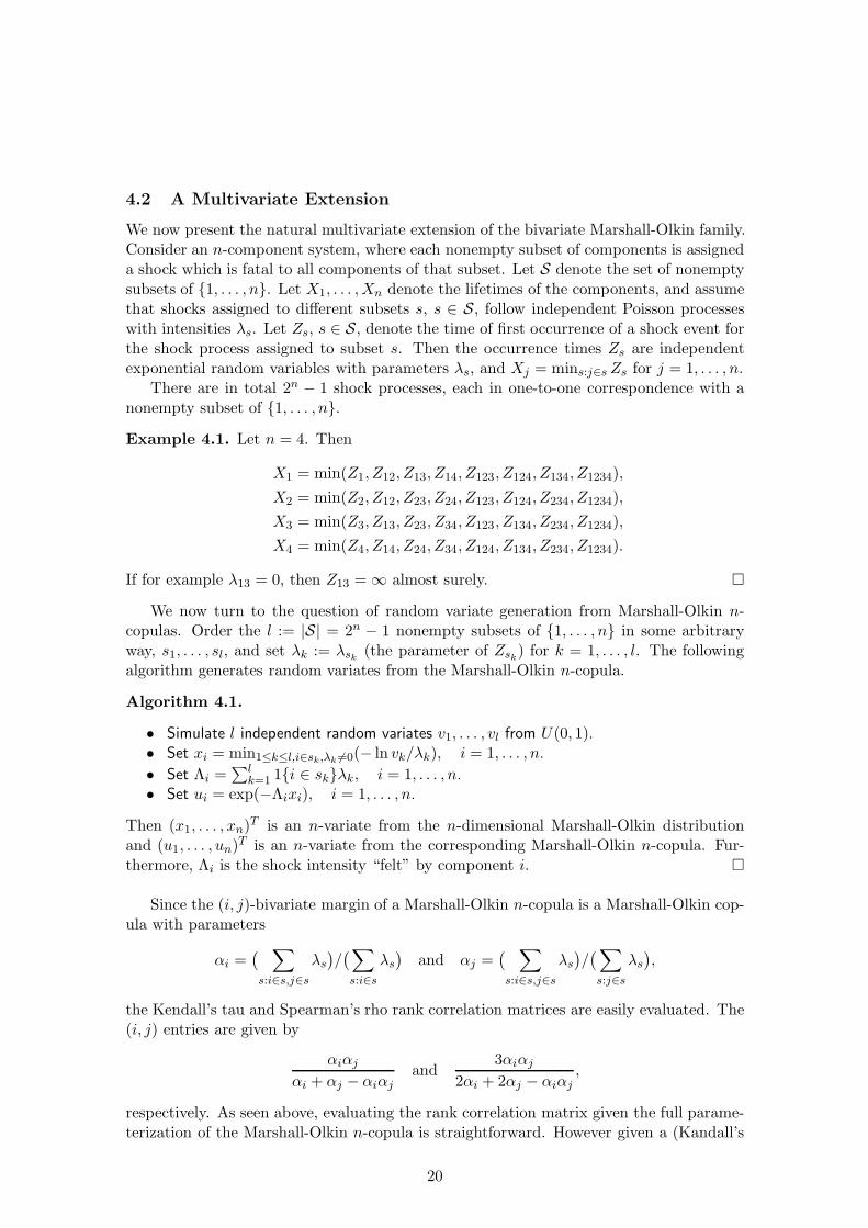
4.2 A Multivariate Extension

We now present the natural multivariate extension of the bivariate Marshall-Olkin family.Consider an n-component system, where each nonempty subset of components is assigneda shock which is fatal to all components of that subset. Let S denote the set of nonemptysubsets of {1, . . . , n}. Let X1, . . . ,Xn denote the lifetimes of the components, and assumethat shocks assigned to different subsets s, s ∈ S, follow independent Poisson processeswith intensities λs. Let Zs, s ∈ S, denote the time of first occurrence of a shock event forthe shock process assigned to subset s. Then the occurrence times Zs are independentexponential random variables with parameters λs, and Xj = mins:j∈sZs for j = 1, . . . , n.

There are in total 2n − 1 shock processes, each in one-to-one correspondence with anonempty subset of {1, . . . , n}.Example 4.1. Let n = 4. Then

X1 = min(Z1, Z12, Z13, Z14, Z123, Z124, Z134, Z1234),X2 = min(Z2, Z12, Z23, Z24, Z123, Z124, Z234, Z1234),X3 = min(Z3, Z13, Z23, Z34, Z123, Z134, Z234, Z1234),X4 = min(Z4, Z14, Z24, Z34, Z124, Z134, Z234, Z1234).

If for example λ13 = 0, then Z13 = ∞ almost surely. �

We now turn to the question of random variate generation from Marshall-Olkin n-copulas. Order the l := |S| = 2n − 1 nonempty subsets of {1, . . . , n} in some arbitraryway, s1, . . . , sl, and set λk := λsk

(the parameter of Zsk) for k = 1, . . . , l. The following

algorithm generates random variates from the Marshall-Olkin n-copula.

Algorithm 4.1.

• Simulate l independent random variates v1, . . . , vl from U(0, 1).• Set xi = min1≤k≤l,i∈sk,λk 6=0(− ln vk/λk), i = 1, . . . , n.

• Set Λi =∑l

k=1 1{i ∈ sk}λk, i = 1, . . . , n.• Set ui = exp(−Λixi), i = 1, . . . , n.

Then (x1, . . . , xn)T is an n-variate from the n-dimensional Marshall-Olkin distributionand (u1, . . . , un)T is an n-variate from the corresponding Marshall-Olkin n-copula. Fur-thermore, Λi is the shock intensity “felt” by component i. �

Since the (i, j)-bivariate margin of a Marshall-Olkin n-copula is a Marshall-Olkin cop-ula with parameters

αi =( ∑s:i∈s,j∈s

λs

)/(∑s:i∈s

λs

)and αj =

( ∑s:i∈s,j∈s

λs

)/(∑s:j∈s

λs

),

the Kendall’s tau and Spearman’s rho rank correlation matrices are easily evaluated. The(i, j) entries are given by

αiαj

αi + αj − αiαjand

3αiαj

2αi + 2αj − αiαj,

respectively. As seen above, evaluating the rank correlation matrix given the full parame-terization of the Marshall-Olkin n-copula is straightforward. However given a (Kandall’s

20

tau or Spearman’s rho) rank correlation matrix we cannot in general obtain a uniqueparameterization of the copula. By setting the shock intensities for subgroups with morethen two elements to zero, we obtain the perhaps most natural parameterization of thecopula in this situation. However this also means that the copula only has bivariatedependence.

4.3 A Useful Modelling Framework

In general the huge number of parameters for high-dimensional Marshall-Olkin copulasmake them unattractive for high-dimensional risk modelling. However, we now give anexample of how an intuitively appealing and easier parameterized model for modellingdependent loss frequencies can be set up, for which the survival copula of times to firstlosses is a Marshall-Olkin copula.

Suppose we are interested in insurance losses occurring in several different lines ofbusiness or several different countries. In credit-risk modelling we might be interested inlosses related to the default of various different counterparties or types of counterparty. Anatural approach to modelling this dependence is to assume that all losses can be relatedto a series of underlying and independent shock processes. In insurance these shocks mightbe natural catastrophes; in credit-risk modelling they might be a variety of underlyingeconomic events. When a shock occurs this may cause losses of several different types; thecommon shock causes the numbers of losses of each type to be dependent. It is commonlyassumed that the different varieties of shocks arrive as independent Poisson processes,in which case the counting processes of the losses are also Poisson and can be handledeasily analytically. In reliability such models are known as fatal shock models, when theshock always destroys the component, and nonfatal shock models, when components havea chance of surviving the shock. A good basic reference on such models is Barlow andProschan (1975).

Suppose there are m different types of shocks and for e = 1, . . . ,m, let {N (e)(t), t ≥ 0}be a Poisson process with intensity λ(e) recording the number of events of type e occurringin (0, t]. Assume further that these shock counting processes are independent. Considerlosses of n different types and for j = 1, . . . , n, let {Nj(t), t ≥ 0} be a counting process thatrecords the frequency of losses of the jth type occurring in (0, t]. At the rth occurrenceof an event of type e the Bernoulli variable I(e)

j,r indicates whether a loss of type j occurs.The vectors

I(e)r = (I(e)

1,r , . . . , I(e)n,r)

T

for r = 1, . . . ,N (e)(t) are considered to be independent and identically distributed witha multivariate Bernoulli distribution. In other words, each new event represents a newindependent opportunity to incur a loss but, for a fixed event, the loss trigger variables forlosses of different types may be dependent. The form of the dependence depends on thespecification of the multivariate Bernoulli distribution with independence as a special case.We use the following notation for p-dimensional marginal probabilities of this distribution(the subscript r is dropped for simplicity):

P (I(e)j1

= ij1 , . . . , I(e)jp

= ijp) = p(e)j1,...,jp

(ij1 , . . . , ijp), ij1 , . . . , ijp ∈ {0, 1}.

We also write p(e)j (1) = p

(e)j for one-dimensional marginal probabilities, so that in the spe-

cial case of conditional independence we have p(e)j1,...,jp

(1, . . . , 1) =∏p

k=1 p(e)jk

. The counting

21

processes for events and losses are thus linked by

Nj(t) =m∑

e=1

N(e)(t)∑r=1

I(e)j,r .

Under the Poisson assumption for the event processes and the Bernoulli assumption forthe loss indicators, the loss processes {Nj(t), t ≥ 0} are clearly Poisson themselves, sincethey are obtained by superpositioningm independent (possibly thinned) Poisson processesgenerated by the m underlying event processes. The random vector (N1(t), . . . ,Nn(t))T

can be thought of as having a multivariate Poisson distribution.The presented nonfatal shock model has an equivalent fatal shock model representa-

tion, i.e. of the type presented in Section 4.2. Hence the random vector (X1, . . . ,Xn)T

of times to first losses of different types, where Xj = inf{t ≥ 0 | Nj(t) > 0}, has ann-dimensional Marshall-Olkin distribution whose survival copula is a Marshall-Olkin n-copula. From this it follows that Kendall’s tau, Spearman’s rho and coefficients of taildependence for (Xi,Xj)T can be easily calculated. For more details on this model, seeLindskog and McNeil (2001).

5 Elliptical Copulas

The class of elliptical distributions provides a rich source of multivariate distributionswhich share many of the tractable properties of the multivariate normal distribution andenables modelling of multivariate extremes and other forms of nonnormal dependences.Elliptical copulas are simply the copulas of elliptical distributions. Simulation from ellip-tical distributions is easy, and as a consequence of Sklar’s Theorem so is simulation fromelliptical copulas. Furthermore, we will show that rank correlation and tail dependencecoefficients can be easily calculated. For further details on elliptical distributions we referto Fang, Kotz, and Ng (1987) and Cambanis, Huang, and Simons (1981).

5.1 Elliptical Distributions

Definition 5.1. If X is a n-dimensional random vector and, for some µ ∈ Rn and some

n × n nonnegative definite, symmetric matrix Σ, the characteristic function ϕX−µ(t) ofX− µ is a function of the quadratic form tTΣt, ϕX−µ(t) = φ(tT Σt), we say that X hasan elliptical distribution with parameters µ, Σ and φ, and we write X ∼ En(µ,Σ, φ). �

When n = 1, the class of elliptical distributions coincides with the class of one-dimensional symmetric distributions. A function φ as in Definition 5.1 is called a charac-teristic generator.

Theorem 5.1. X ∼ En(µ,Σ, φ) with rank(Σ) = k if and only if there exist a randomvariable R ≥ 0 independent of U, a k-dimensional random vector uniformly distributedon the unit hypersphere {z ∈ R

k|zT z = 1}, and an n × k matrix A with AAT = Σ, suchthat

X =d µ+RAU.

For the proof of Theorem 5.1 and the relation between R and φ see Fang, Kotz, and Ng(1987) or Cambanis, Huang, and Simons (1981).

22

Example 5.1. Let X ∼ Nn(0, In). Since the components Xi ∼ N (0, 1), i = 1, . . . , n,are independent and the characteristic function of Xi is exp(−t2i /2), the characteristicfunction of X is

exp{−12(t21 + · · ·+ t2n)} = exp{−1

2tT t}.

From Theorem 5.1 it then follows that X ∼ En(0, In, φ), where φ(u) = exp(−u/2). �

If X ∼ En(µ,Σ, φ), where Σ is a diagonal matrix, then X has uncorrelated components(if 0 < Var(Xi) <∞). If X has independent components, then X ∼ Nn(µ,Σ). Note thatthe multivariate normal distribution is the only one among the elliptical distributionswhere uncorrelated components imply independent components. A random vector X ∼En(µ,Σ, φ) does not necessarily have a density. If X has a density it must be of the form|Σ|−1/2g((X − µ)T Σ−1(X − µ)) for some nonnegative function g of one scalar variable.Hence the contours of equal density form ellipsoids in R

n. Given the distribution ofX, the representation En(µ,Σ, φ) is not unique. It uniquely determines µ but Σ and φare only determined up to a positive constant. More precisely, if X ∼ En(µ,Σ, φ) andX ∼ En(µ∗,Σ∗, φ∗), then

µ∗ = µ, Σ∗ = cΣ, φ∗(·) = φ(·/c),

for some constant c > 0.In order to find a representation such that Cov(X) = Σ, we use Theorem 5.1 to obtain

Cov(X) = Cov(µ+RAU) = AE(R2)Cov(U)AT ,

provided that E(R2) < ∞. Let Y ∼ Nn(0, In). Then Y =d ‖Y‖U, where ‖Y‖ isindependent of U. Furthermore ‖Y‖2 ∼ χ2

n, so E(‖Y‖2) = n. Since Cov(Y) = In we seethat if U is uniformly distributed on the unit hypersphere in R

n, then Cov(U) = In/n.Thus Cov(X) = AAT

E(R2)/n. By choosing the characteristic generator φ∗(s) = φ(s/c),where c = E(R2)/n, we get Cov(X) = Σ. Hence an elliptical distribution is fully describedby µ, Σ and φ, where φ can be chosen so that Cov(X) = Σ (if Cov(X) is defined). IfCov(X) is obtained as above, then the distribution of X is uniquely determined by E(X),Cov(X) and the type of its univariate margins, e.g. normal or t4, say.

Theorem 5.2. Let X ∼ En(µ,Σ, φ), let B be a q × n matrix and b ∈ Rq. Then

b +BX ∼ Eq(b +Bµ,BΣBT , φ).

Proof. By Theorem 5.1, b +BX has the stochastic representation

b +BX =d b +Bµ+RBAU.

Partition X, µ and Σ into

X =(X1

X2

), µ =

(µ1

µ2

), Σ =

(Σ11 Σ12

Σ21 Σ22

),

where X1 and µ1 are r × 1 vectors and Σ11 is a r × r matrix.

23

Corollary 5.1. Let X ∼ En(µ,Σ, φ). Then

X1 ∼ Er(µ1,Σ11, φ), X2 ∼ En−r(µ2,Σ22, φ).

Hence marginal distributions of elliptical distributions are elliptical and of the sametype (with the same characteristic generator). The next result states that the conditionaldistribution of X1 given the value of X2 is also elliptical, but in general not of the sametype as X1.

Theorem 5.3. Let X ∼ En(µ,Σ, φ) with Σ strictly positive definite. Then

X1 | X2 = x ∼ Er(µ, Σ, φ),

where µ = µ1 + Σ12Σ−122 (x− µ2) and Σ = Σ11 −Σ12Σ−1

22 Σ21. Moreover, φ = φ if and onlyif X ∼ Nn(µ,Σ).

For the proof and details about φ, see Fang, Kotz, and Ng (1987). For the extension tothe case where rank(Σ) < n, see Cambanis, Huang, and Simons (1981).

The following lemma states that linear combinations of independent, elliptically dis-tributed random vectors with the same dispersion matrix Σ (up to a positive constant)remain elliptical.

Lemma 5.1. Let X ∼ En(µ,Σ, φ) and X ∼ En(µ, cΣ, φ) for c > 0 be independent. Thenfor a, b ∈ R, aX + bX ∼ En(aµ+ bµ,Σ, φ∗) with φ∗(u) = φ(a2u)φ(b2cu).

Proof. By Definition 5.1, it is sufficient to show that for all t ∈ Rn

ϕaX+bX−aµ−bµ(t) = ϕa(X−µ)(t)ϕb(X−µ)(t)

= φ((at)T Σ(at))φ((bt)T (cΣ)(bt))= φ(a2tT Σt)φ(b2ctT Σt).

As usual, let X ∼ En(µ,Σ, φ). Whenever 0 < Var(Xi),Var(Xj) <∞,

ρ(Xi,Xj) := Cov(Xi,Xj)/√

Var(Xi)Var(Xj) = Σij/√

ΣiiΣjj.

This explains why linear correlation is a natural measure of dependence between randomvariables with a joint nondegenerate (Σii > 0 for all i) elliptical distribution. Throughoutthis section we call the matrix R, with Rij = Σij/

√ΣiiΣjj, the linear correlation matrix

of X. Note that this definition is more general than the usual one and in this situation(elliptical distributions) makes more sense. Since an elliptical distribution is uniquelydetermined by µ, Σ and φ, the copula of a nondegenerate elliptically distributed randomvector is uniquely determined by R and φ.

One practical problem with elliptical distributions in multivariate risk modelling isthat all margins are of the same type. To construct a realistic multivariate distributionfor some given risks, it may be reasonable to choose a copula of an elliptical distributionbut different types of margins (not necessarily elliptical). One big drawback with sucha model seems to be that the copula parameter R can no longer be estimated directlyfrom data. Recall that for nondegenerate elliptical distributions with finite variances, R isjust the usual linear correlation matrix. In such cases, R can be estimated using (robust)

24

linear correlation estimators. One such robust estimator is provided by the next theorem.For nondegenerate nonelliptical distributions with finite variances and elliptical copulas,R does not correspond to the linear correlation matrix. However, since the Kendall’s taurank correlation matrix for a random vector is invariant under strictly increasing transfor-mations of the vector components, and the next theorem provides a relation between theKendall’s tau rank correlation matrix and R for nondegenerate elliptical distributions, Rcan in fact easily be estimated from data.

Theorem 5.4. Let X ∼ En(µ,Σ, φ) with P{Xi = µi} < 1 and P{Xj = µj} < 1. Then

τ(Xi,Xj) = (1−∑x∈R

(P{Xi = x})2) 2π

arcsin(Rij), (5.1)

where the sum extends over all atoms of the distribution of Xi. If rank(Σ) ≥ 2, then (5.1)simplifies to

τ(Xi,Xj) = (1− (P{Xi = µi})2) 2π

arcsin(Rij).

For a proof, see Lindskog, McNeil, and Schmock (2001). Note that if P{Xi = µi} = 0for all i, which is true for e.g. multivariate t or normal distributions with strictly positivedefinite dispersion matrices Σ, then

τ(Xi,Xj) =2π

arcsin(Rij)

for all i and j.The nonparametric estimator of R, sin(πτ/2) (dropping the subscript for simplicity),

provided by the above theorem, inherits the robustness properties of the Kendall’s tauestimator and is an efficient (low variance) estimator of R for both elliptical distributionsand nonelliptical distributions with elliptical copulas.

5.2 Gaussian Copulas

The copula of the n-variate normal distribution with linear correlation matrix R is

CGaR (u) = Φn

R(Φ−1(u1), . . . ,Φ−1(un)),

where ΦnR denotes the joint distribution function of the n-variate standard normal dis-

tribution function with linear correlation matrix R, and Φ−1 denotes the inverse of thedistribution function of the univariate standard normal distribution. Copulas of the aboveform are called Gaussian copulas. In the bivariate case the copula expression can be writ-ten as

CGaR (u, v) =

∫ Φ−1(u)

−∞

∫ Φ−1(v)

−∞

12π(1 −R2

12)1/2exp

{−s

2 − 2R12st+ t2

2(1−R212)

}ds dt.

Note that R12 is simply the usual linear correlation coefficient of the corresponding bi-variate normal distribution. Example 3.4 shows that Gaussian copulas do not have uppertail dependence. Since elliptical distributions are radially symmetric, the coefficient ofupper and lower tail dependence are equal. Hence Gaussian copulas do not have lowertail dependence.

25

We now address the question of random variate generation from the Gaussian copulaCGa

R . For our purpose, it is sufficient to consider only strictly positive definite matrices R.Write R = AAT for some n × n matrix A, and if Z1, . . . , Zn ∼ N (0, 1) are independent,then

µ+AZ ∼ Nn(µ,R).

One natural choice of A is the Cholesky decomposition of R. The Cholesky decompositionof R is the unique lower-triangular matrix L with LLT = R. Furthermore Choleskydecomposition routines are implemented in most mathematical software. This providesan easy algorithm for random variate generation from the Gaussian n-copula CGa

R .

Algorithm 5.1.

• Find the Cholesky decomposition A of R.• Simulate n independent random variates z1, . . . , zn from N (0, 1).• Set x = Az.• Set ui = Φ(xi), i = 1, . . . , n.• (u1, . . . , un)T ∼ CGa

R .

As usual Φ denotes the univariate standard normal distribution function. �

5.3 t-copulas

If X has the stochastic representation

X =d µ+√ν√S

Z, (5.2)

where µ ∈ Rn, S ∼ χ2

ν and Z ∼ Nn(0,Σ) are independent, then X has an n-variatetν-distribution with mean µ (for ν > 1) and covariance matrix ν

ν−2Σ (for ν > 2). If ν ≤ 2then Cov(X) is not defined. In this case we just interpret Σ as being the shape parameterof the distribution of X.

The copula of X given by (5.2) can be written as

Ctν,R(u) = tnν,R(t−1

ν (u1), . . . , t−1ν (un)),

where Rij = Σij/√

ΣiiΣjj for i, j ∈ {1, . . . , n} and where tnν,R denotes the distributionfunction of

√νY/

√S, where S ∼ χ2

ν and Y ∼ Nn(0, R) are independent. Here tν denotesthe (equal) margins of tnν,R, i.e. the distribution function of

√νY1/

√S. In the bivariate

case the copula expression can be written as

Ctν,R(u, v) =

∫ t−1ν (u)

−∞

∫ t−1ν (v)

−∞

12π(1 −R2

12)1/2

{1 +

s2 − 2R12st+ t2

ν(1−R212)

}−(ν+2)/2

ds dt.

Note that R12 is simply the usual linear correlation coefficient of the corresponding bi-variate tν -distribution if ν > 2.

If (X1,X2)T has a standard bivariate t-distribution with ν degrees of freedom andlinear correlation matrix R, then X2 | X1 = x is t-distributed with v + 1 degrees offreedom and

E(X2 | X1 = x) = R12x, Var(X2 | X1 = x) =(ν + x2

ν + 1

)(1−R2

12).

26

This can be used to show that the t-copula has upper (and because of radial symmetry)equal lower tail dependence:

λU = 2 limx→∞P(X2 > x | X1 = x)

= 2 limx→∞ tν+1

( ν + 1ν + x2

)1/2 x−R12x√1− ρ2

l

= 2 lim

x→∞ tν+1

((ν + 1

ν/x2 + 1

)1/2 √1−R12√1 +R12

)= 2tν+1

(√ν + 1

√1−R12/

√1 +R12

).

From this it is also seen that the coefficient of upper tail dependence is increasing in R12

and decreasing in ν, as one would expect. Furthermore, the coefficient of upper (lower)tail dependence tends to zero as the number of degrees of freedom tends to infinity forR12 < 1.Coefficients of upper tail dependence for the bivariate t-copula are:

ν\R12 -0.5 0 0.5 0.9 12 0.06 0.18 0.39 0.72 14 0.01 0.08 0.25 0.63 1

10 0.00 0.01 0.08 0.46 1∞ 0 0 0 0 1

The last row represents the Gaussian copula, i.e. no tail dependence.It should be mentioned that the expression given above is just a special case of a

general formula for the coefficient(s) of tail dependence for elliptical distributions withtail dependence. It turns out that if Σii > 0 for all i and −1 < Σij/

√ΣiiΣjj < 1 for all

i 6= j, then the bivariate marginal distributions of an elliptically distributed random vectorX =d µ + RAU ∼ En(µ,Σ, φ) has tail dependence if and only if R is so-called regularlyvarying (at ∞). For more details, see Hult and Lindskog (2001), and for details aboutregular variation in general see Resnick (1987) or Embrechts, Mikosch, and Kluppelberg(1997).

Equation (5.2) provides an easy algorithm for random variate generation from thet-copula, Ct

ν,R.

Algorithm 5.2.

• Find the Cholesky decomposition A of R.• Simulate n independent random variates z1, . . . , zn from N (0, 1).• Simulate a random variate s from χ2

ν independent of z1, . . . , zn.• Set y = Az.• Set x =

√ν√sy.

• Set ui = tν(xi), i = 1, . . . , n.• (u1, . . . , un)T ∼ Ct

ν,R.

�

27

••••• •

•••••

•

••••••

••

••

• •••••

• •••

••••• •••

•••• ••

••• ••

•••••

•••••

••• •• •••• •••• ••••••• •••••••

••• ••••• •• ••• •••• ••• •••••••• •••

••• •

•• • •••••

••• •••

• ••• •••• •••••

••• • • ••••• ••••

•••• •

••••• ••

••••••

••

••• •••• ••••

•••• •••

••

•

•••••••

••

•• •••

••

••••

•• •••• •

•••••• ••

•••

• ••••••••••

•

•

••••

• •••• •••

••

•• ••

•

•• •• •

• ••••

•

• •••• •

••••

•• •••

•••••••

•••••• •

• ••

•• ••

••

•• ••• • •••• • ••

• •• •• • • •••• ••• •• •• •• •

••• •••• • ••• ••• •• •••

•••• •

••

••••

••

•••••••••

•••• • ••• ••••

•

•

•

•••• •

••

•

•

•

•

••

•

•••

••

• • ••

•

••• •• ••

•••

•• •

••

•••

•

••

• ••••

••

•

•

••

••

••• • ••

•• ••

•• •••

•••

•••••

•••

• •••••••

••

••

••••••

••

••

••••

••

•

• •••••• •

• •• •• ••••

•••

•••• •• •

••

• •••

••

••

••

•• • ••

• • ••• ••

•

•• •••• • ••• ••••

••••• •••

••••••••• •• • ••

•••• ••••••

• ••••• •••••

••

•• ••

•• ••••

••• ••••••• ••••••••••••••••• ••

•

•• •

••••••••• •••• •••••• •• •••••• ••••••••• • ••••••••• ••••• ••• •

•• •••••• •••••

• •••• ••••• •• ••••• •• • ••• •••• •

••• ••

•••••• ••

•• • ••• •••• • ••• ••• ••••• •••

••••••••

•• ••• •• ••••••••• ••• • •

• ••••• ••••••••• • •• •••• •••

• •• •••• • •••••••••• ••••••••••• ••• •••••••• •• •

•••

••• ••

•• ••••• •• •••••

•• ••••• ••

•• •

••• ••••

•

••• ••••

• •• ••••

••

• •• •

••• •• •• •

••••• •• •

• •• •••

••• ••••••••• ••••• ••••• • •

• •• •••••

•••••

•• •••

•• ••••••

•••

•• •• ••••

•••••••••• ••••••••• • •• •

••••••

•• ••••

••••• •• ••••••••• ••• ••• •••• ••••••• • •• ••••••••• ••• •••• ••• • •• ••••

• ••• ••• • ••

••

••• • ••• •••• • •

•• ••• ••••

•••• ••

••••

• • ••• • •••••• ••• • •••

••

•••• •••

•••••• ••

•• ••••••• • •

••

•••• ••••

••• •••

• ••• •• •••• •••

•••••• ••

•••

•••

•• ••• •• •••

•

• •• •••• ••••

••••••

••

••

•••

••• ••• ••••

••••• ••

• ••••• •••

••

•• •• •••• •••••

•

•••••

•• •••

• ••••• •• • ••• •• ••••

••

•••••

••• ••

••• •

•

•• ••• •••

• ••• • ••• •• •••

•••

••

•••••••• ••

•••••••••• • •••••••• •••••• ••••• ••

••

• ••

••• •• •

•••• ••

•

•••

••

••

••••••

•••

••• ••• ••

••

••••

•• • ••••• •••

•••

•••••••••

••• •• •• •••

••• •

•••• • •••

•• • ••• •••

••• •••••

••• •••

•••• •• ••• ••••• •

••

•• •••• •••

•••••••

•• ••••• •• •

• •• • ••• ••• •••••• •••

•••••• •••••• ••••••••••••

•• •• •• •

•••••••••

•••• •

•• •••• ••

••••••••••••• ••• •••• ••••••••

•• •

• •• ••••

••••• ••

••••

•••••

••• •••• ••• • •• •• ••••• •••• ••• • •• • •• •••••• •••••• • •••• ••••• ••••• •

••• •••

••• •••• • ••••

•••• •• ••••• •• •

•••

•• •• •• ••••••• ••• ••• •••

••• ••• ••• •

• ••••••••• ••• • ••••••• ••••• ••• ••••• •••••••• •• •••• • •

•••••

••

•••••

BMW-Siemens

-15 -10 -5 0 5 10

-15

-10

-50

510

••

•• • •••••• •• • •••

•••••• ••

•• •

•••• •••

•• ••• •••

•

••• •••• •••••

••• •

••

••

• •• ••

••• • ••••• •

•

• ••

•••

•

••• ••

• •••••••• •

••

••

• •• •••

••• ••••••••••••

••••••••

•• •

•••

• ••

•• ••

•• ••

••••

••

•

••

••

••••

• •

•

•• •••••

•• •

•••

•••• ••

•••

• ••

•

•

••

•• ••••

•• •••• ••

••• • •••

•

••

••••••••

•• ••

•

•••

••• •••••

•••

•••

• •

•

••

•

••••••••

••••• •••••

•• ••

•

•• ••• ••• ••••

••• • •••• •

•••

••••

• ••• •••

• ••• •••

••

•

• ••

••••• •••

•••• •

••

• ••••••• ••

••• ••

• ••

• ••

••

•••

•••• • •

••••

••••

•••

••

••••

•

• ••• ••

• ••••• •

••••

•••

••

• ••••

••

•••• •

••• •• •••

•••

••• • ••

•• •

•••

•••

• •••••

••

•• ••

•••

•••• ••

•

••••• •••••

•••

•••••

••

•

•

•

•••••• •••••

••• ••••

••

••• • •

•

•

•

••••

•• •••

••

••••• ••

••

• • •••• •

••

••

••••••••

•••

•

••

•••••••

••

•••• •

••• •• ••

• • •• ••

• ••••••••

•••••

••••••

•

••

•••

•••••

• •

••

•• ••••• ••• •

••

•

•••

• •••••• •• •

•••••

••

• •• ••••

••

• •• •• •

• ••• •

• ••

•

••

•••••

••••

••

• • •••••

••••• ••

••••

•

••••• •••

••• •• • ••

•

• •••

••••

•••

••

• •••• ••••••• ••••

• ••••• •

••••

•••••

• •••• ••

•• •• • •

•••

••

•• ••

••••

•••

•

•• ••• ••••

••

• •••

•••• ••• •

••

••• ••••

•••

•

•

•••••

•• ••••• •••• ••••• •••

•••••• ••• •••

• •••••••

•••

•••

••••••

••

•• ••••

•••

•••••••

•• •••••

•••• ••

•

••

• ••• •

•••

•••• ••••

••• ••

••• •

•

•• •••

•• •• •

• ••••

•

••••• •••

•• •••

•••••••• • •

•• • •

••••

• ••••

•

• ••• ••• ••

••• •• ••••

••

•

••••

•••••

••••

•

• •

•

••••••

••••••••

••

••• •• •••• •••

•

• •••••

• • •• •

•••

••• ••••

••••• •••••••

••• ••

••

•••• • •

••• ••• • ••••••••••••

••

••• ••• •••

•• •• •••

••••••

•••• ••• •

• ••••

•••••

•••••• •••

••• ••••

•••

•• •••••••••

•

••• •

••••• •

•••• ••• •

••

•• •• ••

•••

•

• ••••

•••• •

•••

•••• ••••

••••

•••

••

•• ••• •• •••

•••

••

••

•••

•• ••••••• •• •

•••••

• •• ••

•••••

••• ••

••

•••

••••• •••••

•••

••• •••

••••••••

•••• •

••••

••

•• ••

• ••

• ••• ••• •••••••••••••••

•• •••

••

••

•

•

•

••••••

••

• •••

•••••••••

•••••

•••••

••••

•••

•• ••

•••

•

••

• ••••

••••••••

••

•••

•

••

•••

••

••

•• ••••

••

•• • ••• ••

••••••••

•• ••••

• •

•

••

• ••••••••••

•••••

••

••

•• •

•••

•

•• ••• •• • ••• •• •

••••••••••••

•••••••

•

••• ••••

•••••••••

•

•• •

••• •••••• ••• ••

•••••••

•• •

•• •••

• •• ••

•

•••• •••••••• •••

••••• ••

••

•• •••

•••• ••••

••

•• •• ••• •

••• •• ••• ••

•

••

••••

• • •••••

••

•• • •

• •• •• ••••••• •• • ••• •

••

•

•

•••••••••••

••••

••

••••••

•

• •••

•

•• ••

•• •••• •• • ••••• •••• ••• ••

••• •••••

••

• •••

•

• • •

•••

• • ••••

•

••••••••••

•••••• ••••

•••

••

•

••• •• ••••• •• ••••

••

••

•••

••

••• ••

••

•• •

••• ••• ••••

••••

• •• •

••

• •

••• ••••• • •

•••

•

••••• •• •• •

•••• •

• •• •••

• •••••• •• •• ••••• •••

• •••

••••• •

•••• •••

••• •••••••

•

t2

-15 -10 -5 0 5 10

-15

-10

-50

510

•••••

••

•••

•••

••

•• •

••

••••• ••

••••

•• ••• •••

••• ••• ••• •

•• •••

•• ••••• •••• •

••••

•• • •••

•••••

••• •

•••••

••

••

•••

• ••

••

••• ••• •• •

•

• •••••

• •••••

••••

••••••••

•

•• ••••

•••• ••••

•••

•••

••

••• • •• •• ••

••••

•

•••

•

•• •• ••••••• •

• ••••

••

••••

••

••••••• • •

••

•••••••

••• ••• •

••

••• •• •••••• • ••• ••••••

••••• ••

••••• ••••••••••••

••

•••

• •••

••••

•

•

••

•••••

•••• ••••••••• ••••

• •••••• •••

••

•• •••••

••••• ••

•

• • •• •

••• •• ••

••

•

•

••• • • ••• •••• ••

• ••••

•••••••

•• •

••••• •••

•• ••••

••

••

••••• ••• •••

•

•• ••

••••• ••

•

• ••••••

••••

•• • ••• •• ••

• ••• ••

••••• •••

•• • •• •

••••

•• ••• ••

••

•••

• •••• •••

••

•••• •

•••

•

•••

• • ••••••••••• ••

•••

•

••••• •• •••

•••

•

• •• •••••

• ••••

••••• •••••

••

•• •

•••••

••••

••

•••••

•• •

• •••

••• •

••••••••••

•••• ••

•

••

••••••

•••

•••••

••

•••

•••

•••

•••••••• •••

••• •• • ••• ••••••• •••

•• •••••

••

• •• •••• •••

•• •• ••••

••

••

• •••••••• •

•

•• • •

••••

•••

•

•••

•

••••

•• ••• •• •• •

•

•• •• •

••

••

•••• •••

••••

•• • •••

• •••

•• •• •••••• ••

••••

••

••••• •• •• •••••• ••••• •••• ••

•••

••• ••• ••••• •••

••

•

•••• ••••

••• ••

•

•

•

•••••••

•••• ••• •• •

••••• •

•

•••

•••

••••

•• •••• •••• ••••

••• ••

•••• ••• ••

••

••••

••

••••••

•••• •••

•

••

••• •• ••• •••

••••••

•••

•• ••• • ••• • •

• ••

•••••••

•• •• •••••• •• •••

••

••• •• • ••

• •••••••••••

••• •

•••

• ••• • • •• •

•

••• •••

• •••••• •••••• •••• ••• •••• •••••

••••• •

•••

••• ••••

•••

••••

•••

••••

••••

• •••• •••••• •• •

••• •

•

•••

•••

• • • •• •

•

••

••

••

•••••

•• ••

•• ••••• •••

•• ••

•••• ••••• ••

••

•••••

•••• •

•

• •••••

••••• •• •••

••

•

••

•• •••••

•• ••••

•••

• •• ••

• •••••••

•

•••

•••

•••••

• • ••••• •

••

••

•••••

••• ••

••

•• •• •••

••• •

•

••

••••

•

• ••••• •

•••

•••• ••••

• •••••• • ••••••••

• •• ••••

••

•••• ••• •• ••••• •

••••• •••

•••

•

•

• • •••• • •••• •

••••

•

••

••

••

•

••

• •••••••••••

•

•••

•• •••

•• ••

•• ••• •

••••

•••••

••• ••• •

•

•

•• •• • ••

•• •••••

••

•••

•••• • •

••••• •••

•••• ••••••

•

••

•• •••

• •••••••••• ••••

•

•••••• •

•

•••

••• •

•• ••

•••••••

•••• • ••

••••••••••• • •

•••••

••

•••

•

••••

••• ••••

••• •••

•••

••

••• ••••• • •• •

••••

•••• ••••• •

•• ••• • ••••

••

•••

••

•• ••

••••••• •

•••• ••••••

•• ••• •••••

•• ••

• •••

•

•••••

•••• •

•

•• •••

•• • •

••• ••

•• •

• •• ••

••

•

••• • •• •••••••• ••

•

••• •• •• •

•••• ••

•••• ••

••••••

••••

••••

• ••

•••• ••

•

•••

••• •• •••• •

••• ••

•

•••• •••• ••• •• •••• •••

•

••••

••••

•••• ••

•••• ••

••

•••••

•• ••

•••

•

••••• •

••••••• ••••••

•• •••

•

••• •

•

•• ••••

•

•

••

••••

•••

• ••

•••• • •• ••• •

•• ••

••

••• ••

•

•••

•••

•• •

•

• •••••

••••• ••

•••• •

•••• •••••

•••• ••

• ••• •• ••• •

• •• ••••

• ••• •• ••

••

••• •••

•

•••••

• •• ••

Gaussian

-15 -10 -5 0 5 10

-15

-10

-50

510

••

•

••••••

•• •

••••

•

••• •••• ••

•• ••••• • ••

•• •••

••••

••

•• •

••• ••• •

•••••

••

• •••••••

• •••••• ••

•••••

• •••

••

••• ••••

•

••• ••

• •• ••••

•••• ••• •

•• •••

•

• • ••

••

•

••••

••

••• • •

•• ••

••

••••

•• • •• ••••

••• • •••

••••

•••

•••

••

•

•

•• ••

•

••

•

•••• • •• ••••

••

• •••••••

••• •• ••

•••••

• ••• • ••

•

•

•• ••••••

• ••

•• •

•• •• •

•••• •• •• •

••• •

•• ••• ••• •••

•

••

•

•••• ••••

• • •••• •• •• ••••••

•••

•• •••

•• •

••••• •• •••

••• •

•

•••••

•

••

•

•••

•• •••

•• •

•••

••••

•• •••••• •

•••• ••••

••• ••

•••••

••••

•

•••

• ••••

•• ••

••

•• •••

•

••

••

••

• ••

•

•

•• ••

•• ••

•

•

••• •••

••

•

•

• ••• ••• •

•••••• •••••

•••

•• •• •• •

•

•••••••• •

••• • •••

••

•

•••

•••••••

•••• ••• •

•••

••••••••

••

••••

••

••

•• •

••••••••••••••

• ••

•••••

••

• •••

•• • •• • ••• ••••

• •• •••••

•• •

••••

•

• ••

•• •

•• ••• •••• • •••••• •••

••

•• ••

••••

•••

•••

••

••

••• •

• •• ••• ••••

•••••

•• •• ••

•••• ••••

••

••

•

•• ••

••

••••••

••• •

•••

• ••••••••

• ••••

•• •••

• ••

•

••

•

••

• •••••

••••••

••• ••

••

•••• •

•••

••

••• •• •••

••••

•••••••• •••

••• ••

• •

•

••

••••••• ••• • •

•

•

••• • •••••••••• •

•••• •

•••••

••••• ••• •• •••••

••••

•

••• •••• ••

••• ••

• ••• • •••

•• •••• • •••••

•••••••

•• ••••• •• •••

••• •••

•••

•••• ••••

••••

• •

••••

••• •• •

•

••

••••• • ••

•• ••••

• •

••

•

•••

• ••••

•

• ••••••

••• ••

•• ••••• •

• •••

••• •••

•

••••

• ••••••••

•• ••••••••

••••••••

••••• •• •••

•• •••• ••••• ••• ••• •• ••••

•

•••

••••

•

••••••••

••

•••• ••

••••••••

•

• ••

• ••• ••

•••• • ••

••••• ••

••

•••• ••

•• •••• ••• •••••

••• •• ••

•• •• •

••••••

••• •

•

• • •••

• •••• •••••• ••••••

•• • •

••••

•••

•• ••• • •••• •••••

•

•• •••••

••••

••

•

• •

•

•••

•• ••

• ••••

••

••

•••

••• •

••

••

•• •••••

•••

••

••

••• •

•

•

•••• •••••

•••• •• •

• •• ••••••••••

••

•••

••••

•••

•• ••

••••

••

••• ••

•

•••

••

• •• •••

• •••••• •

•

•

•••

••••••

••••••

•••••

••

•••••••

• •••

•••• •••

•••••

••

••

••• ••

••••• ••••••

• •• ••

•••••

••• •• •••••

••

••••• •• •

•••••

••••

•

••

•••••

•••• ••

•••• •

••

•• •

••

••• •••

••••• •

••

••••

• •••• •••

••••

•••••• ••

••• ••

••

•• •••

•••

••

•• • • ••• •• •• ••••

•

••••

•••••

••• ••••• •

•••••

•••

•••

••

••••

•

•

••• • ••

• ••• •

••

••

••

••

•••

•••• •

••• • ••• ••

•••• •

•••••••

•••

•••

•

•• ••••• •

•• •

• ••• •••• •••• •

•• ••

•

••

••••••• •••• •••

•••• •••

•••• •• ••• •••••••

•••••

••

•• •••

••• ••

•

•••

•••••• ••••

••• •

••••

• ••••

•• • ••

• ••••• • ••

•• ••• •••••• •• •• •

•••

••••••

••• ••• ••

• ••• ••

••

••••••

•••• ••

•• •• •

•••••

•• •••• •••• ••• ••• •

• •••• ••••

••••• •

••

• ••••

•••••••

• •• •

•

••••••••• •

•••••

••• •••••• •••

•

•• •• ••

•

•

••••• ••••

•• • •• ••••

•••• • •

•

••• •••

••••

•

•• • ••

• ••••

• •• • •• •

••

••••

••

••••• ••• •••

•

• ••

••

••••• ••

Gumbel

-15 -10 -5 0 5 10

-15

-10

-50

510

Figure 5.1: The upper left plot shows BMW-Siemens daily log returns from 1989 to 1996.The other plots show samples from bivariate distributions with t4-margins and Kendall’stau 0.5.

28

••

•

•

•

•

•

•

••• •

•

•

•

•

•

• ••

•

•

•

•

••

•

••

•

•

••

•

••

•••

•

•

•

•

•

••

•

•

•

•

•

•

•

•

••

••

•

•

••

•

•

•

••

•

•

• •

•

•

•

•

••

••

•

•

•

• •

•

•

••

•

•

•

•

•

•

••

•

•

•

•

•

••

•

•

•

••

•

••

•

•

••

•

•

•

•• •

•

•

•

••

•

•

•

•

••• ••

••

•

••

•

••

••

•

•

•

•

•

•

•

•

••

•

••

•

•

•

•

• •

•

•

••

•

•

•

•

•

••

••

••

•

•

•

•

•

•

•

•

•

•

•

•

•

•

•

•

•

•

•

•

•

•

•

•

•

•

•

••

•

•••

•

•

•••

•

•

•

•

••

•

•

•

•

•

•

•

••

•

•

•

•

•

•

•

•

•

••

•

•

•

•

•

•

••

•

•

•

•

•

•

••

•

••

•

••

••

•

•

•

•

•

•

•

•

•

•

••

••

•

•

•

•

•

•

•

•

•

•

•

•

••

•

•

•

•

•

••

•

•

• •

•

•

•

• •

•

•

•

•

•

•

•

••

•

•

•

•

•

•

•

•

•

•

•

•

•

••

•

••

•

•

•

•

•

•

•

•

•

•

•

••

•

•

•

•

•

•

•

•

•

••

•••

•

•

•

•

••

•

•

•

••

•

•

•

•

•

•

•

••

•

•••

•

•

•

•

•

••

•

•

••

•

•

•

•

•

•

•

•

••

••

•

•

•••

••

•

••

•

•

•

•

•

•

•

•

•• •

•

•

•

••

•

•

•

••

••

•

•

•

•

••

•

•

••

•

•

•

••

••

•

•

•

• •

•

•

•

•

••

•

••

•

•

•

•

•

•

•

•• •

•

•

•

•

•••

•

•

•• ••

•

•

•

•

•

•

• •

•

•

•

•

•

•

•

•

••

•

•

••

•

•

••

•

•

•

•

•

•

•

•

•• •

•

•••

•

•••

•

•

••

•

•

•

•

• •

•

••

•

•

•

•

•

••

•

•

•

•

•

••

•

•

•

•

•••

•

••

•

•

•

•

•

•

•

• ••

•••

•

••

•

•

•

•

•

•

•

•

•

•

••

•

•

•

•

•

•

•

• •

•

•

•

•

•

•••

•

•

•

••

•

•

•

•

•

•

•

•

• ••

•

••

•

••

•

•

•

•

•

•

••

••

•

•

•

••

•

••

•• •

• ••

••

•

••

•

•

•

•

• •

•

•

•

•

•

•

•

•

•

•

•

•

•

•

•

•

•

•

•

•

•

• •

•

••

•

••

••

•

•

•

•

•

•

•

•

•

••

•

••

•

•

•

•

•

•

••

•

•

•

•

•

• •

•

•

••

•

•

•

•

••

•

•

•

••

•

•

•

•

•

•

•

•

••

•

•

•

•

•

••

••

••

•

••

•

•

• •

•

•

••

•

•

• ••

•

•

•

••

••

•

•

••

•

•

•

•

•

•

•

•••

•

•

•

•

••

•

•

••

•

•

•

•

••

•

•

•

•

•

•

•

•

••

•

•

•

•

•

•

•

•

•

••

•

•

••

•

•

•

•

•

•

••

•

••

• •

•

•

•

••

•

•

•

•

•

•

•

•

•

•

•

•

•

•

•

••

•

• •

•

•

•

•

•••

••

•

•

•

•

• •

•

•

•

•

•

•

•

•

•

•

•

•

•• ••

•

•

•

•

•

••

•

••

•

•

•

•••

••

•

••

•

•

••

•

•

•

•

•

•

•

••

•

•

•

•

••

•

•

••

••

•

•

•

•

••

•

•

•

•

•

•

•

•

•

•

•

•

•

•

•

•

•

•

•

•

•

•

•

•

•

•

•

•

•

•

•

•

•

•

• •

••

•

•

•

•

•

••

••

•

•

•

•

• •••

•

•

•

•

•

•

•

•

•

••

•

•

••

•

••

•

•

•

•

•

••

•

•

•

•

•

• ••

•••

•

•

•

•

••

•

•

•

••

•

•

••

•

•

•

•

••

••

•

•

•

•

•

•

•••

••

•

•

•

•

•• •

•

•

••

••

•

•

•

••

•

•

•

••

•

•

•

• •

••

•

••

••

•

•

•

•

•

•

•

•

•

• •

•

•

•••

•

•

••

•

••

•

••

•

•

•

•••

•

•

•

•

•

•

••

•

••

•

•

•

•

•

•

••

•

•

•••

••

•• •

••

•

•

•

•

•

•

•

••

•

•

•

•

••

•

•

•

•

•

•

•

•

•

• •

•

••

••

•

•

•

•

•

•

••

•

••

••

•

•

•

•

•

•

•

•

•

•

•

•

•

•

•

•

•

••

••

•

••

••

•

•

•

•

•

•

•

•

•

•

•

•

•

•

•

•

••

•

•

•

•

•

•

• • •

•

• •

•

•

•

•

•

•

•

••

•

•

•

•

•

••

•

•

•

•

•

•

•

•

•

••

•

•

•

•

•

•

••

•

•

•

•

•

•

•

•

•

•

••

• •

••

••

•

•

•

•

•••

•

•

•

••

•

•

•

•

•

•

•

•

•

•••

•••

•

•

•

•

•

•

•

•

•

•

•

•

•

•

•

•

•

•••

•

•

•

•

•

•

•••

•

•

•

•

•

•

•

•

•

•

•

•

• •

•

••

••

•

•

•

•••

•

•

••

•

•

•

•

•

•

••

•

•

•

••

••

•

•

•

•••

•

•

•

•

•

•

••

•

•

•

•

•

•

•

•

••

•

•

•

••

•

•

•••

•

•

•

•

•

•

•

•

•

•

••

•

•

•

•

•

•

•

•

•

•

••

•

•

•

• •

•

•

•

•

••

•

•

•

•

•

•

••

•

• ••

• •

•

••

•

•

••

•

•

•

•

• •

•

••

•

•

•

•

• •

•

•

•

•

•

••

•••

•

•

••

•

•

•

•

•

•

•

•

•

•

•

•

•

•

••

•

•

•

••

•

•

•

••

•

••

•••

•

••

•

••

•

•

•

•

•

•

•

•

•

•

•

••

•

•

•

•

•

•

•

•

•

•

•

•••

•

• ••

•

••

•

•

••

•

• •

••

•

•

•

•

• •

•

•

•

••

•

•

•

•

•

•

•

••

•

•

•

•

•

•

•

• •

•

•

••

•

•

•

••

•••

•

•

•

•

•

•

•

•

•

•

•

••

•

•

•

•

•

•

••

•

•

•

•

•

•

•

• ••

•

•

•• •

••

•

•

•• ••

•

•

•

•••

•

••

• •

•

•••

•

•

•

•

•

•

•

•

•

•

•

•

•

•

••

•

•

•

••

•

•

•

•

••

••

•

•

•• •••

•

••

•

•

•

•

•

••

•

•

••

•

•

•

•

•

••

• •

••

•

•

•

••

•

•

•

••

•

••

••

•

•

•••

•

••

•

•

•

••

•

•

•

•

•• •

•

••

•

•

••

•

•

••

•

•

•

•

•

•

•

••

•

•

•

•

•

••

• ••

•

•

•

•

•

••

• •

•

•

•

•

•

•

•

•

•

•

•

•

•

•

••

•••

••

•

••

•

•

•

•

•

• •

••

•

•

•

•

••

•

•

•

•

•

•

•

•

••

•

•

•

••

•

•

••

•

•

•

••

•••• •

•

•

•

•

•

•

••

•

•

••

•

•

• •••

•

• •

•

•

•

•

•

•

••

•

•

•

•

•

•

•

•

•

•

•

•

•

•

Gaussian

X1

Y1

-4 -2 0 2 4

-4-2

02

4

••

•

•

•

•

•

•

•

•

•

•

•

•

•

•

•

•

•

•

•

•

•

•

••

•

••

•

••

••

•

•

••

•

••

•

•

•

•

•

••

•

•

•

••

•

• •

•

•

•

•

•

•

•

•

•

•

•

•

•

•

•

•

•

••

•

•

•

•

••

••

•

•

•

•

•

•

•

•

•

•

•

••

•

•

•

•

•

•

•

•

•

•

•

•

•

•

•

•

•

•

•

•

•

•

•

••

••

•

•

•

•

••

••

•

•

•

•

•

•

•

•

•

•

•

•

• ••

•

•

•• •

•

•

•

•

•

•

•

•

• •

•

•

•

•

•

••

•

•

•

•

•

•

•

•

•

•

•

•

•

•

• ••

•

•

••

•

•

•

•

•

•

•

•

•

••

•

•

•

•

•

••

•

•

•

••

•

•

•

•

•

•

•

•

•

•

•

•

•

•

•

•

•

•

•

•

•

•

••

•

•

••

•

••

•

•

•

••

•

•

•

•

•

•

•

•

•

••

••

•

•

•

•••

•

•••

•

•

•

•

•

••

•

•

•

•

• ••

••

•

•

•

••

•

•

•

•

•

• •

•

•

•

•

•

•

•

•

•

•

••

•

•

•

•

•

•

••

••

•

•

••

•

•

•

•

• •

•

•

•

•

••

•

•

•

••

•

•• •

•

•

•

•

•

•

•

••

•

•

•

•

•

•

•

•

••

•

••

•

•

•

•

•

•

•

•

• •

•

•• •••

•

•

••

••

•

••

•

•••

•

••

••

•

•

•

•• •

••

••

••

••

•

•

•

•

•

•

•

••

•

•

•

•

••

•

•

•

•

•

•

•

•

•

•

•

•

•

•

••

•

•

•

••

•

•

•

••

•

•

• •••

•

•

•

••

•

•

•

•

•

•

•

•

•

•

•

•

• •

••

•

••

••

•

•

•

•

••

•

•

•

•••

••

••

•

•

• ••

•

•

•

•

•

•

••

•

••

•

••

•

•

•

•

•

•

•

•

•

•

••

•

•

•

•

••

•

•

• •

•

•

•

•

•

•

•

••

•

•

•

•

•

•

• •

•

•

•

•

•

•

•

• •

•

•

•

•

•

•

•

•

•

•

• •

•

•

•

•

•

•

•

•

•

•

•

•

•

••

•

••

•

•

•

••

••

•

•

••

•

••

•

•

•

•

••

•

•

•

•

•

•

••

•

•

• •

••

•

•

•

•

•

•

•

•

•

•

•

•

•

••

•

•

•

•

••

•

•

•

•

•

•••

•

•••

•

•• •

•

•

••

•

•

•

•

•

•

•

•

•

••

•

•

•

••

•

•

•

••

•

•

•

•

•

•

•

•

••

•

•

••

•

• •

•

•

•

•

•

•

• •

•

•

•

•

•

•

• •

•

•

•

•

•

•

•

•

•

•

•

•

•

•

••

•

•

•

•

•

•

••

••

•

•

•

•

•

•

••

•

•

•

•

•

•

•

•

•

•••

••

••

•

••

•

•

•

•

•

•

•

•

•

•

•

••

••

•

•

•

•

•

•

••

•

•

•

••

•

•

•

•

•

•

•

•

•

••

••

•

•

••

•

•

•

•

•

•

••

•

•

•

• ••••

•

•

•

•

•

•

•

•

•

•

•

•

•

•

••

•

•

•

•

• ••

•

• ••

•

•

••

••

•

•

•

•

•

•

•

•

•

•

•

••

••

•

•

•

•

•

••

•

•

•

•

•

•

•

•

•

•

•

• •• ••

•

•

••

•••

•

•

••

•

•

•

•

••

•

•

••• ••

•

•

•

•

•

•

•

• ••

•

•

•

•

•

•

••

•

•

••

• •• •

•

• ••

•

•

•

••

•

••

•

••

•

•

•

•

•

•

•

•

•

•

•

•

•••

•

••

• •

•

•

•

•

•

•

•••

•

•

•

•

•

•

•

•

•

•

•

•

•

•

•

•

•

••••

•

•

••

•

•

•

••

•

••

•

••

•

•

•

•

•

•

•••

•

•

•

•

•

•

•

•

•

•

•

•

•

••

•

•

••

•

•

•

•

•

••

•

••

•

•

•

•

•

•

•

•

•

•

•

•

•

••

•

•

•

•

•

•

•

•

•••

••

•

•

•

•

•

•

•

•

•

•

•

•

•

•

•

•••

•

•••

•

• •••

•

•

•

••

•

•

•

•

•

•

•

•

•

•

•

•

•• ••

•

•

•

•

•

•

••

•

•

•

••

•

•

•

•

•

• •

•

•

•

• •

•

•

•

•

••

•

•

••

•

•

•

•

•

••

•

•

•

•

•

•

••

•

•

•

•

••

•

•

•

•••

•

••

•

•

••

••

•

•

•

•

•

•

•

•

••

••

•

•

••

•

••

•

•

•

•

•

•

•

•

••

•

•

••

••

•

•

••

•

••

•

•

•

•

•

•

• •

•

•

•

•

••

•

•

•

•

•

•••

•

•

•

•••

•

•

•

••

•

•

••

•

•

••

•

•

•

•

••

•

••

•

•

••

•

•

•

•

•

•

•

•

••

•

• •

•

•

•

•

••

•

••

•

•

•

••

•

•

•

•

•

•

••

•

•

•

•

•

•

•

•

•

•

•

••

•

•

••

•

•

•

•

• ••

•

•

•

•

•

•

••

•

•

•

•

•

•

••

•

•

•

•••

•

•••

•

•

•

•

•

•

•

•

•

•

•

••

• •

• •

•

•

•

•

•

•

••

•

•

•

•

•

••

•

• •

•

••

•

•

•

•

•

•

•

•

•

•

•

•

•

•

••

• •

•

•

•

••

•

••

•

•

•

•

•

•

•

••

•

•

•

••

••

•

•

•

•

•

•

••

•

••

••

• •

•

•

•

••

•

•

•

••

•

•

•

•

• •

•

•

••

•

•

•

•

•

•

•

••

•

•

•

•

•

••

•

•

••

•

••

•

••

•

•

•

•

•

•

•

••

•

•

•

•

•

•

••

•

••

••

••

•

••

•

•

•

•

•

•

• •

•

•

•

•

•• •

•

•

•

•

•

•

•

•

••

•

•

•

•

••

••

•

•• •

•

•

•

•

•

•

•

••

•

•

•

•

•

•

• •

•

•

•

•

•

••

••

• •

•

••

•

•

•

•

•

• •

•

••

•

•

•

•

•

•

•

•

•••

••

•

•

•

•

•

••••

••

••

•

• •

•

•

•

• •

•

•

•

•

•

•

•

••

•

•

• •

••

••

•

•

•

••

• •

•

•

•

••

••

•

•

•

•

••

•

•

•

•

•• ••

•

•

•

•

•

•

•

•

•

•

•

•

•

•

•

• •

•

•

•

•

•

•

•

•

•

•

••

•

•

••

••

••

••

•

•

•

•

•

•

•

•

•

•

•

•

• •

•

•

•

•

••

•

••

• ••

••

•

••

••

••

•

•

• •

•

•••

••

•

••

•

••

•

•

•

•

•

•

•

•

•

•

•

•

•

•

•

•

••

•

•

••

•

•

•

•

•

•

••

•

•

•

•

•

•

•

•

•

•

•

•

•

•

•

••

•

•

•

••

••

•

•

•

•••

•

•

•

•

•

•

•

•

••

•

•

•

•

•

•

•

••

•

•

• •

•••

•

••

•

••

•••

•

•

•

•

•

•

•

•

•

•

••

••

•

•

•

••

•

•

•

•

•

•

•

•

•

•

•

•• •

•

•

••

•

•

••

•••

•

•

••

•

•

•

••

•

•••

•

•

•

•

•

•

• •

••

•

•

•

•

••

•

•

•

•

•

t

X2

Y2

-4 -2 0 2 4

-4-2

02

4

Figure 5.2: Samples from two distributions with standard normal margins, R12 = 0.8 butdifferent dependence structures. (X1, Y 1)T has a Gaussian copula and (X2, Y 2)T has at2-copula.

29

Figures 5.1 and 5.2 show samples from bivariate distributions with Gaussian and t-copulas. In Figure 5.1, we have contrasted a real example (BMW-Siemens daily returndata) with simulated data using marginal t4 tails, corresponding Kendall’s tau (0.5) andvarying copulas. Note that the Gaussian copula does not get the extreme joint tail ob-servations clearly present in the real data. The t2-copula seems to be able to do a muchbetter job in that respect. Indeed the t2-generated scatter plot shows most of the graphicalfeatures in the real data. Note that these examples were only introduced to highlight thesimulation procedures and do not constitute a detailed statistical analysis. Figure 5.2 (asimulated example) further highlights the difference between the Gaussian and t-copulas,this time with standard normal margins.

The algorithms presented for the Gaussian and t-copulas are fast and easy to imple-ment. We want to emphasize the potential usefulness of t-copulas as an alternative toGaussian copulas. Both Gaussian and t-copulas are easily parameterized by the linearcorrelation matrix, but only t-copulas yield dependence structures with tail dependence.

6 Archimedean Copulas

The copula families we have discussed so far have been derived from certain families ofmultivariate distribution functions using Sklar’s Theorem. We have seen that ellipticalcopulas are simply the distribution functions of componentwise transformed ellipticallydistributed random vectors. Since simulation from elliptical distributions is easy, so issimulation from elliptical copulas. There are however drawbacks: elliptical copulas donot have closed form expressions and are restricted to have radial symmetry (C = C).In many finance and insurance applications it seems reasonable that there is a strongerdependence between big losses (e.g. a stock market crash) than between big gains. Suchasymmetries cannot be modelled with elliptical copulas.

In this section we discuss an important class of copulas called Archimedean copulas.This class of copulas is worth studying for a number of reasons. Many interesting para-metric families of copulas are Archimedean and the class of Archimedean copulas allow fora great variety of different dependence structures. Furthermore, in contrast to ellipticalcopulas, all commonly encountered Archimedean copulas have closed form expressions.Unlike the copulas discussed so far these copulas are not derived from multivariate distri-bution functions using Sklar’s Theorem. A consequence of this is that we need somewhattechnical conditions to assert that multivariate extensions of Archimedean 2-copulas areproper n-copulas. A further disadvantage is that multivariate extensions of Archimedeancopulas in general suffer from lack of free parameter choice in the sense that some of theentries in the resulting rank correlation matrix are forced to be equal. At the end of thissection we present one possible multivariate extension of Archimedean copulas. For othermultivariate extensions we refer to Joe (1997).

There is much written about Archimedean copulas. For some background on bivariateArchimedean copulas see Genest and MacKay (1986b). For parameter estimation anda discussion on other statistical questions we refer to Genest and Rivest (1993). Goodreferences on Archimedean copulas in general are Genest and MacKay (1986a), Nelsen(1999) and Joe (1997). See also the webpage http://www.mat.ulaval.ca/pages/genest/for further related work.

30

6.1 Definitions

We begin with a general definition of Archimedean copulas, which can be found in Nelsen(1999) p. 90. As our aim is the construction of multivariate extensions of Archimedean2-copulas, this general definition will later prove to be a bit more general than needed.

Definition 6.1. Let ϕ be a continuous, strictly decreasing function from [0, 1] to [0,∞]such that ϕ(1) = 0. The pseudo-inverse of ϕ is the function ϕ[−1] : [0,∞] → [0, 1] givenby

ϕ[−1](t) ={ϕ−1(t), 0 ≤ t ≤ ϕ(0),0, ϕ(0) ≤ t ≤ ∞.

�

Note that ϕ[−1] is continuous and decreasing on [0,∞], and strictly decreasing on[0, ϕ(0)]. Furthermore, ϕ[−1](ϕ(u)) = u on [0, 1], and

ϕ(ϕ[−1](t)) ={t, 0 ≤ t ≤ ϕ(0),ϕ(0), ϕ(0) ≤ t ≤ ∞.

Finally, if ϕ(0) = ∞, then ϕ[−1] = ϕ−1.

Theorem 6.1. Let ϕ be a continuous, strictly decreasing function from [0, 1] to [0,∞]such that ϕ(1) = 0, and let ϕ[−1] be the pseudo-inverse of ϕ. Let C be the function from[0, 1]2 to [0, 1] given by

C(u, v) = ϕ[−1](ϕ(u) + ϕ(v)). (6.1)

Then C is a copula if and only if ϕ is convex.

For a proof, see Nelsen (1999) p. 91.Copulas of the form (6.1) are called Archimedean copulas. The function ϕ is called a

generator of the copula. If ϕ(0) = ∞, we say that ϕ is a strict generator. In this case,ϕ[−1] = ϕ−1 and C(u, v) = ϕ−1(ϕ(u) + ϕ(v)) is said to be a strict Archimedean copula.

Example 6.1. Let ϕ(t) = (− ln t)θ, where θ ≥ 1. Clearly ϕ(t) is continuous and ϕ(1) = 0.ϕ′(t) = −θ(− ln t)θ−1 1

t , so ϕ is a strictly decreasing function from [0, 1] to [0,∞]. ϕ′′(t) ≥ 0on [0, 1], so ϕ is convex. Moreover ϕ(0) = ∞, so ϕ is a strict generator. From (6.1) we get

Cθ(u, v) = ϕ−1(ϕ(u) + ϕ(v)) = exp(−[(− ln u)θ + (− ln v)θ]1/θ).

Furthermore C1 = Π and limθ→∞Cθ = M (recall that Π(u, v) = uv and M(u, v) =min(u, v)). This copula family is called the Gumbel family. As shown in Example 3.3 thiscopula family has upper tail dependence. �

Example 6.2. Let ϕ(t) = (t−θ − 1)/θ, where θ ∈ [−1,∞) \ {0}. This gives the Claytonfamily

Cθ(u, v) = max([u−θ + v−θ − 1]−1/θ, 0).

For θ > 0 the copulas are strict and the copula expression simplifies to

Cθ(u, v) = (u−θ + v−θ − 1)−1/θ. (6.2)

The Clayton family has lower tail dependence for θ > 0, and C−1 = W , limθ→0Cθ = Πand limθ→∞Cθ = M . Since most of the following results are results for strict Archimedeancopulas we will refer to (6.2) as the Clayton family. �

31

Example 6.3. Let ϕ(t) = − ln e−θt−1e−θ−1

, where θ ∈ R \ {0}. This gives the Frank family

Cθ(u, v) = −1θ

ln(

1 +(e−θu − 1)(e−θv − 1)

e−θ − 1

).

The Frank copulas are strict Archimedean copulas. Furthermore limθ→−∞Cθ = W ,limθ→0Cθ = Π and limθ→∞Cθ = M . Members of the Frank family are the only Archimedeancopulas which satisfy the equation C(u, v) = C(u, v) for so-called radial symmetry, seeFrank (1979) for details. �

Example 6.4. Let ϕ(t) = 1− t for t in [0, 1]. Then ϕ[−1](t) = 1 − t for t in [0, 1], and 0for t > 1; i.e., ϕ[−1](t) = max(1 − t, 0). Since C(u, v) = max(u+ v − 1, 0) =: W (u, v), wesee that the bivariate Frechet–Hoeffding lower bound W is Archimedean. �

6.2 Properties

The results in the following theorem will enable us to formulate multivariate extensionsof Archimedean copulas.

Theorem 6.2. Let C be an Archimedean copula with generator ϕ. Then1. C is symmetric, i.e. C(u, v) = C(v, u) for all u, v in [0, 1].2. C is associative, i.e. C(C(u, v), w) = C(u,C(v,w)) for all u, v,w in [0, 1].

Proof. The first part follows directly from (6.1). For 2.,

C(C(u, v), w) = ϕ[−1](ϕ(ϕ[−1](ϕ(u) + ϕ(v))) + ϕ(w))= ϕ[−1](ϕ(u) + ϕ(v) + ϕ(w))= ϕ[−1](ϕ(u) + ϕ(ϕ[−1](ϕ(v) + ϕ(w)))) = C(u,C(v,w)).

The associativity property of Archimedean copulas is not shared by copulas in generalas shown by the following example.

Example 6.5. Let Cθ be a member of the bivariate Farlie-Gumbel-Morgenstern familyof copulas, i.e. Cθ(u, v) = uv + θuv(1− u)(1 − v), for θ ∈ [−1, 1]. Then

Cθ

(14, Cθ

(12,13

))6= Cθ

(Cθ

(14,12

),13

)for all θ ∈ [−1, 1]\{0}. Hence the only member of the bivariate Farlie-Gumbel-Morgensternfamily of copulas that is Archimedean is Π. �

Theorem 6.3. Let C be an Archimedean copula generated by ϕ and let

KC(t) = VC({(u, v) ∈ [0, 1]2 | C(u, v) ≤ t}).

Then for any t in [0, 1],

KC(t) = t− ϕ(t)ϕ′(t+)

. (6.3)

For a proof, see Nelsen (1999) p. 102.

32

Corollary 6.1. If (U, V )T has distribution function C, where C is an Archimedean copulagenerated by ϕ, then the function KC given by (6.3) is the distribution function of therandom variable C(U, V ).

The next theorem will provide the basis for a general algorithm for random variategeneration from Archimedean copulas. Before the theorem can be stated we need anexpression for the density of an absolutely continuous Archimedean copula. From (6.1) itfollows that

ϕ′(C(u, v))∂

∂uC(u, v) = ϕ′(u),

ϕ′(C(u, v))∂

∂vC(u, v) = ϕ′(v),

ϕ′′(C(u, v))∂

∂uC(u, v)

∂

∂vC(u, v) + ϕ′(C(u, v))

∂2

∂u∂vC(u, v) = 0,

and hence

∂2

∂u∂vC(u, v) = −

ϕ′′(C(u, v))∂

∂uC(u, v)

∂

∂vC(u, v)

ϕ′(C(u, v))= −ϕ

′′(C(u, v))ϕ′(u)ϕ′(v)[ϕ′(C(u, v))]3

.

Thus, when C is absolutely continuous, its density is given by

∂2

∂u∂vC(u, v) = −ϕ

′′(C(u, v))ϕ′(u)ϕ′(v)[ϕ′(C(u, v))]3

. (6.4)

Theorem 6.4. Under the hypotheses of Corollary 6.1, the joint distribution functionH(s, t) of the random variables S = ϕ(U)/[ϕ(U) + ϕ(V )] and T = C(U, V ) is givenby H(s, t) = sKC(t) for all (s, t) in [0, 1]2. Hence S and T are independent, and S isuniformly distributed on [0, 1].

Proof. (This proof, for the case when C is absolutely continuous, can be found in Nelsen(1999) p. 104. For the general case, see Genest and Rivest (1993).) The joint densityh(s, t) of S and T is given by

h(s, t) =∂2

∂u∂vC(u, v)

∣∣∣∂(u, v)∂(s, t)

∣∣∣,where ∂2C(u, v)/∂u∂v is given by (6.4) and ∂(u, v)/∂(s, t) denotes the Jacobian of thetransformation ϕ(u) = sϕ(t), ϕ(v) = (1− s)ϕ(t). But

∂(u, v)∂(s, t)

=ϕ(t)ϕ′(t)ϕ′(u)ϕ′(v)

,

and hence

h(s, t) =(−ϕ

′′(t)ϕ′(u)ϕ′(v)[ϕ′(t)]3

)(− ϕ(t)ϕ′(t)ϕ′(u)ϕ′(v)

)=ϕ′′(t)ϕ(t)[ϕ′(t)]2

.

Therefore

H(s, t) =∫ s

0

∫ t

0

ϕ′′(y)ϕ(y)[ϕ′(y)]2

dydx = s

[y − ϕ(y)

ϕ′(y)

]t

0

= sKC(t),

from which the conclusion follows.

33

An application of Theorem 6.4 is the following algorithm for generating random vari-ates (u, v)T whose joint distribution is an Archimedean copula C with generator ϕ.

Algorithm 6.1.

• Simulate two independent U(0, 1) random variates s and q.

• Set t = K−1C (q), where KC is the distribution function of C(U, V ).

• Set u = ϕ[−1](sϕ(t)) and v = ϕ[−1]((1 − s)ϕ(t)).

Note that the variates s and t correspond to the random variables S and T in Theorem6.4 and from the proof it follows that this algorithm yields the desired result. �

Example 6.6. Consider the Archimedean copula family given by

Cθ(u, v) =(1 +

[(u−1 − 1)θ + (v−1 − 1)θ

]1/θ)−1

generated by ϕθ(t) = (t−1−1)θ for θ ≥ 1. To generate a random variate from C we simplyapply Algorithm 6.1 with

ϕθ(t) = (t−1 − 1)θ,ϕ−1

θ (t) = (t1/θ + 1)−1,

K−1Cθ

(t) =θi + 1

2−√(θi + 1

2)2 − θis.

�

6.3 Kendall’s tau Revisited

Recall that Kendall’s tau for a copula C can be expressed as a double integral of C.This double integral is in most cases not straightforward to evaluate. However for anArchimedean copula, Kendall’s tau can be expressed as an (one-dimensional) integralof the generator and its derivative, as shown in the following theorem from Genest andMacKay (1986a).

Theorem 6.5. Let X and Y be random variables with an Archimedean copula C generatedby ϕ. Kendall’s tau of X and Y is given by

τC = 1 + 4∫ 1

0

ϕ(t)ϕ′(t)

dt. (6.5)

Proof. Let U and V be U(0, 1) random variables with joint distribution function C, andlet KC denote the distribution function of C(U, V ). Then from Theorem 3.3 we have

τC = 4E(C(U, V ))− 1 = 4∫ 1

0t dKC(t)− 1

= 4(

[tKC(t)]10 −∫ 1

0KC(t) dt

)− 1 = 3− 4

∫ 1

0KC(t) dt.

From Theorem 6.3 and Corollary 6.1 it follows that

KC(t) = t− ϕ(t)ϕ′(t+)

.

34

Since ϕ is convex, ϕ′(t+) and ϕ′(t−) exist for all t in (0, 1) and the set {t ∈ (0, 1) | ϕ′(t+) 6=ϕ′(t−)} is at most countable (i.e. it has Lebesgue measure zero). Hence

τC = 3− 4∫ 1

0

(t− ϕ(t)

ϕ′(t+))dt = 1 + 4

∫ 1

0

ϕ(t)ϕ′(t)

dt.

Example 6.7. Consider the Gumbel family with generator ϕ(t) = (− ln t)θ, for θ ≥ 1.Then ϕ(t)/ϕ′(t) = (t ln t)/θ. Using Theorem 6.5 we can calculate Kendall’s tau for theGumbel family.

τθ = 1 + 4∫ 1

0

t ln tθ

dt = 1 +4θ

([ t22

ln t]10−∫ 1

0

t

2dt)

= 1 +4θ(0− 1/4) = 1− 1/θ.

As a consequence, in order to have Kendall’s tau equal to 0.5 in Figure 5.1 (the Gumbelcase), we put θ = 2. �

Example 6.8. Consider the Clayton family with generator ϕ(t) = (t−θ − 1)/θ, for θ ∈[−1,∞) \ {0}. Then ϕ(t)/ϕ′(t) = (tθ+1 − t)/θ. Using Theorem 6.5 we can calculateKendall’s tau for the Clayton family.

τθ = 1 + 4∫ 1

0

tθ+1 − t

θdt = 1 +

4θ

(1

θ + 2− 1

2

)=

θ

θ + 2.

�

Example 6.9. Consider the Frank family presented in Example 6.3. It can be shownthat (see e.g. Genest (1987)) Kendall’s tau is τθ = 1− 4(1−D1(θ))/θ, where Dk(x) is theDebye function, given by

Dk(x) =k

xk

∫ x

0

tk

et − 1dt

for any positive integer k. �

6.4 Tail Dependence Revisited

For Archimedean copulas, tail dependence can be expressed in terms of the generators.

Theorem 6.6. Let ϕ be a strict generator such that ϕ−1 belongs to the class of Laplacetransforms of strictly positive random variables. If ϕ−1′(0) is finite, then

C(u, v) = ϕ−1(ϕ(u) + ϕ(v))

does not have upper tail dependence. If C has upper tail dependence, then ϕ−1′(0) = −∞and the coefficient of upper tail dependence is given by

λU = 2− 2 lims↘0

[ϕ−1′(2s)/ϕ−1′(s)].

35

Proof. (This proof can be found in Joe (1997), p. 103.) Note that

limu↗1

C(u, u)/(1 − u) = limu↗1

[1− 2u+ ϕ−1(2ϕ(u))]/(1 − u)

= 2− 2 limu↗1

ϕ−1′(2ϕ(u))/ϕ−1 ′(ϕ(u))

= 2− 2 lims↘0

[ϕ−1′(2s)/ϕ−1′(s)].

If ϕ−1′(0) ∈ (−∞, 0), then the limit is zero and C does not have upper tail dependence.Since ϕ−1′(0) is the negative of the expectation of a strictly positive random variable,ϕ−1′(0) < 0 from which the conclusion follows.

The additional condition on the generator ϕmight seem somewhat strange. It will howeverprove quite natural when we turn to the construction of multivariate Archimedean copulas.Furthermore, the condition is satisfied by the majority of the commonly encounteredArchimedean copulas.

Example 6.10. The Gumbel copulas are strict Archimedean with generator ϕ(t) =(− ln t)θ. Hence ϕ−1(s) = exp(−s1/θ) and ϕ−1′(s) = −s1/θ−1 exp(−s1/θ)/θ. Using Theo-rem 6.6 we get

λU = 2− 2 lims↘0

[ϕ−1′(2s)/ϕ−1′(s)] = 2− 21/θ lims↘0

[exp(−(2s)1/θ)exp(−s1/θ)

]= 2− 21/θ,

see also Example 3.3. �Theorem 6.7. Let ϕ be as in Theorem 6.6. The coefficient of lower tail dependence forthe copula C(u, v) = ϕ−1(ϕ(u) + ϕ(v)) is equal to

λL = 2 lims→∞[ϕ−1′(2s)/ϕ−1′(s)].

The proof is similar to that of Theorem 6.6.

Example 6.11. Consider the Clayton family given by Cθ(u, v) = (u−θ + v−θ − 1)−1/θ,for θ > 0. This strict copula family has generator ϕ(t) = (t−θ − 1)/θ. It follows thatϕ−1(s) = (1 + θs)−1/θ. Using Theorem 6.6 and 6.7 shows that λU = 0 and that thecoefficient of lower tail dependence given by

λL = 2 lims→∞[ϕ−1′(2s)/ϕ−1′(s)] = 2 lim

s→∞

[(1 + 2θs)−1/θ−1

(1 + θs)−1/θ−1

]= 2 · 2−1/θ−1 = 2−1/θ.

�Example 6.12. Consider the Frank family given by

Cθ(u, v) = −1θ

ln(

1 +(e−θu − 1)(e−θv − 1)

e−θ − 1

)for θ ∈ R \ {0}. This strict copula family has generator ϕ(t) = − ln e−θt−1

e−θ−1. It follows that

ϕ−1(s) = −1θ ln(1− (1− e−θ)e−s) and ϕ−1′(s) = −1

θ (1− e−θ)e−s/(1− (1− e−θ)e−s). Since

ϕ−1′(0) = −eθ − 1θ

is finite, the Frank family does not have upper tail dependence according to Theorem 6.6.Furthermore, members of the Frank family are radially symmetric, i.e. C = C, and hencethe Frank family does not have lower tail dependence. �

36

6.5 Multivariate Archimedean Copulas

In this section we look at the construction of one particular multivariate extension ofArchimedean 2-copulas. For other multivariate extensions see Joe (1997). It should benoted that in order to show that other multivariate extensions are proper copulas, weessentially have to go through the same arguments as those given below.

The expression for the n-dimensional product copula Πn, with u = (u1, . . . , un)T , canbe written as Πn(u) = u1 . . . un = exp(−[(− ln u1)+ · · ·+(− lnun)]). This naturally leadsto the following generalization of (6.1):

Cn(u) = ϕ[−1](ϕ(u1) + · · ·+ ϕ(un)). (6.6)

In the 3-dimensional case,

C3(u1, u2, u3) = ϕ[−1](ϕ ◦ ϕ[−1](ϕ(u1) + ϕ(u2)) + ϕ(u3)) = C(C(u1, u2), u3),

and in the 4-dimensional case,

C3(u1, . . . , u4) = ϕ[−1](ϕ ◦ ϕ[−1](ϕ ◦ ϕ[−1](ϕ(u1) + ϕ(u2)) + ϕ(u3)) + ϕ(u4))= C(C3(u1, u2, u3), u4) = C(C(C(u1, u2), u3), u4).

Whence in general, for n ≥ 3, Cn(u1, . . . , un) = C(Cn−1(u1, u2, . . . , un−1), un). This tech-nique of constructing higher-dimensional copulas generally fails. But since Archimedeancopulas are symmetric and associative it seems more likely that Cn as defined above, givencertain additional properties of ϕ (and ϕ[−1]), is indeed a copula for n ≥ 3.

Definition 6.2. A function g(t) is completely monotone on the interval I if it has deriva-tives of all orders which alternate in sign, i.e. if it satisfies

(−1)kdk

dtkg(t) ≥ 0

for all t in the interior of I and k = 0, 1, 2, . . . . �

If g : [0,∞) 7→ [0,∞) is completely monotone on [0,∞) and there is a t ∈ [0,∞) suchthat g(t) = 0, then g(t) = 0 for all t ∈ [0,∞). Hence if the pseudo-inverse ϕ[−1] of anArchimedean generator ϕ is completely monotone, then ϕ[−1](t) > 0 for all t ∈ [0,∞) andhence ϕ[−1] = ϕ−1.

The following theorem from Kimberling (1974) gives necessary and sufficient conditionsfor the function (6.6) to be an n-copula.

Theorem 6.8. Let ϕ be a continuous strictly decreasing function from [0, 1] to [0,∞] suchthat ϕ(0) = ∞ and ϕ(1) = 0, and let ϕ−1 denote the inverse of ϕ. If Cn is the functionfrom [0, 1]n to [0, 1] given by (6.6), then Cn is an n-copula for all n ≥ 2 if and only if ϕ−1

is completely monotone on [0,∞).

This theorem can be partially extended to the case where ϕ is nonstrict and ϕ[−1] ism-monotone on [0,∞) for some m ≥ 2, that is, the derivatives of ϕ[−1] alter sign up to andincluding the mth order on [0,∞). Then the function Cn given by (6.6) is an n-copulafor 2 ≤ n ≤ m. However, for most practical purposes, the class of strict generators ϕ suchthat ϕ−1 is completely monotone is a rich enough class.

The following corollary shows that the generators suitable for extensions to arbitrarydimensions of Archimedean 2-copulas correspond to copulas which can model only positivedependence.

37

Corollary 6.2. If the inverse ϕ−1 of a strict generator ϕ of an Archimedean copula C iscompletely monotone, then C � Π, i.e. C(u, v) ≥ uv for all u, v in [0, 1].

For a proof, see Nelsen (1999) p. 122.While it is simple to generate n-copulas of the form given by (6.6), they suffer from

a very limited dependence structure since all k-margins are identical, they are distri-bution functions of n exchangeable U(0, 1) random variables. One would like to havea multivariate extension of the Archimedean 2-copula given by (6.1) which allows fornonexchangeability. Such multivariate extensions are discussed in Joe (1997). We willnow discuss one such extension in detail. Since any multivariate extension should contain(6.6) as a special case, clearly the necessary conditions for (6.6) to be a copula has to besatisfied. In the light of Theorem 6.8, we restrict ourselves to strict generators.

The expression for the general multivariate extension of (6.1) we will now discussis notationally complex. For that reason we will discuss sufficient conditions for the 3-and 4-dimensional extensions to be proper 3- and 4-copulas respectively. The pattern andconditions indicated generalize in an obvious way to higher dimensions. The 3-dimensionalgeneralization of (6.1) is

ϕ−11 (ϕ1 ◦ ϕ−1

2 (ϕ2(u1) + ϕ2(u2)) + ϕ1(u3)), (6.7)

where ϕ1 and ϕ2 are generators of strict Archimedean copulas. The 4-dimensional gener-alization of (6.1) is

ϕ−11 (ϕ1 ◦ ϕ−1

2 (ϕ2 ◦ ϕ−13 (ϕ3(u1) + ϕ3(u2)) + ϕ2(u3)) + ϕ1(u4)), (6.8)

where ϕ1, ϕ2 and ϕ3 are generators of strict Archimedean copulas. The expressions (6.7)and (6.8) can be written as C1(C2(u1, u2), u3) and C1(C2(C3(u1, u2), u3), u4), respectively,where Ci denotes an Archimedean copula generated by ϕi.

If generators ϕi are chosen so that certain conditions are satisfied, then multivariatecopulas can be obtained such that each bivariate margin has the form (6.1) for some i.However, the number of distinct generators ϕi among the n(n− 1)/2 bivariate margins isonly n− 1, so that the resulting dependence structure is one of partial exchangeability.

Clearly the generators have to satisfy the necessary conditions for the n-copula givenby (6.6) in order to make (6.7) and (6.8) valid copula expressions. What other conditionsare needed to make these proper copulas? To answer that question we now introducefunction classes Ln and L∗n. Let

Ln = {φ : [0,∞) → [0, 1] | φ(0) = 1, φ(∞) = 0, (−1)jφ(j) ≥ 0, j = 1, . . . , n},n = 1, 2, . . . ,∞, with L∞ being the class of Laplace transforms of strictly positive randomvariables.

Also introduce

L∗n = {ω : [0,∞) → [0,∞) | ω(0) = 0, ω(∞) = ∞, (−1)j−1ω(j) ≥ 0, j = 1, . . . , n},n = 1, 2, . . . ,∞. Note that ϕ−1 ∈ L1 if ϕ is the generator of a strict Archimedean copula.The functions in L∗n are usually compositions of the form ψ−1 ◦ φ with ψ, φ ∈ L1.Note also that with this notation, the necessary and sufficient conditions for (6.6) to bea proper copula is that ϕ−1 ∈ Ln and that, if (6.6) is a copula for all n, then ϕ−1 mustbe completely monotone and hence be a Laplace transform of a strictly positive randomvariable.

38

It turns out that if ϕ−11 and ϕ−1

2 are completely monotone (Laplace transforms ofstrictly positive random variables) and ϕ1 ◦ϕ−1

2 ∈ L∗∞, then (6.7) is a proper copula. Notethat (6.7) has (1, 2) bivariate margin of the form (6.1) with generator ϕ2 and (1, 3) and(2, 3) bivariate margins of the form (6.1) with generator ϕ1. Also (6.6) is the special case of(6.7) with ϕ1 = ϕ2. The 3-dimensional copula in (6.7) has a (1, 2) bivariate margin copulawhich is larger than the (1, 3) and (2, 3) bivariate margin copulas (which are identical).

As one would expect, there are similar conditions for the 4-dimensional case. If ϕ−11 ,

ϕ−12 and ϕ−1

3 are completely monotone (Laplace transforms of strictly positive randomvariables) and ϕ1 ◦ ϕ−1

2 and ϕ2 ◦ ϕ−13 are in L∗∞, then (6.8) is a proper copula. Note that

all 3-dimensional margins of (6.8) have the form (6.7) and all bivariate margins have theform (6.1). Clearly the idea underlying (6.7) and (6.8) generalize to higher dimensions.

Example 6.13. Let ϕi(t) = (− ln t)θi with θi ≥ 1 for i = 1, . . . , n, i.e. the generators ofGumbel copulas. What conditions do we have to impose on θ1, . . . , θn in order to obtainan n-dimensional extension of the Gumbel family of the form indicated above (expressions(6.7) and (6.8)). It should first be noted that ϕ−1

i ∈ L∞ for all i, so (6.6) with the abovegenerators gives an n-copula for all n ≥ 2. Secondly, ϕi ◦ϕ−1

i+1(t) = tθi/θi+1. If θi/θi+1 /∈ N,then the nth derivative of ϕi ◦ ϕ−1

i+1(t) is given by

θi

θi+1. . .

(θi

θi+1− (n− 1)

)tθi/θi+1−n.

Hence if θi/θi+1 /∈ N, then ϕi ◦ ϕ−1i+1 ∈ L∗∞ if and only if θi/θi+1 < 1. If θi/θi+1 ∈ N,

then ϕi ◦ ϕ−1i+1 ∈ L∗∞ if and only if θi/θi+1 = 1. Hence an n-dimensional extension of the

Gumbel family of the form indicated above, given by

exp{−([(− ln u1)θ2 + (− lnu2)θ2 ]θ1/θ2 + (− lnu3)θ1)1/θ1}in the 3-dimensional case, is a proper n-copula if θ1 ≤ · · · ≤ θn. �Example 6.14. Consider the Archimedean copula family given by

Cθ(u, v) =(1 +

[(u−1 − 1)θ + (v−1 − 1)θ

]1/θ)−1

generated by ϕθ(t) = (t−1 − 1)θ for θ ≥ 1. Set ϕi(t) = ϕθi(t) for i = 1, . . . , n. Can the

above copulas be extended to n-copulas of the form indicated by (6.7) and (6.8), and ifso under what conditions on θ1, . . . , θn? By calculating derivatives of ϕ−1

i and ϕi ◦ ϕ−1i+1

it follows that ϕ−1i ∈ L∞ and ϕi ◦ ϕ−1

i+1 ∈ L∗∞ if and only if θi/θi+1 ≤ 1. Hence then-dimensional extension of the above copulas are n-copulas if θ1 ≤ · · · ≤ θn.

Copulas of the above form have upper and lower tail dependence, with coefficients ofupper and lower tail dependence given by 2 − 21/θ and 2−1/θ respectively. One limitingfactor for the usefulness of this copula family might be that they only allow for a limitedrange of positive dependence, as seen from the expression for Kendall’s tau given byτ = 1− 2

3θ , for θ ≥ 1. �Note that the results presented in this section hold for strict Archimedean copulas.

With some additional constraints most of the results can be generalized to hold also fornonstrict Archimedean copulas. However for practical purposes it is sufficient to onlyconsider strict Archimedean copulas. This basically means (there are exceptions suchas the Frank family) that we consider copula families with only positive dependence.Furthermore, risk models are often designed to model positive dependence, since in somesense it is the “dangerous” dependence: assets (or risks) move in the same direction inperiods of extreme events.

39

7 Modelling Extremal Events in Practice

7.1 Insurance Risk

Consider a portfolio consisting of n risks X1, . . . ,Xn, representing potential losses in dif-ferent lines of business for an insurance company. Suppose that the insurance company,in order to reduce the risk in its portfolio, seeks protection against simultaneous big lossesin different lines of business. One suitable reinsurance contract might be the one whichpays the excess losses Xi − ki for i ∈ B ⊆ {1, . . . , n} (where B is some prespecified set ofbusiness lines), given that Xi > ki for all i ∈ B. Hence the payout function f is given by

f((Xi, ki); i ∈ B) =

(∏i∈B

1{Xi>ki}

)(∑i∈B

(Xi − ki)

). (7.1)

In order to price this contract the seller (reinsurer) would typically need to estimateE(f((Xi, ki); i ∈ B)). Without loss of generality let B = {1, . . . , l} for l ≤ n. If thejoint distribution H of X1, . . . ,Xl could be accurately estimated, calculating the expectedvalue of (7.1) (possibly by using numerical methods) would not be difficult. Unfortunately,accurate estimation of H is seldom possible due to lack of reliable data. It is more realistic,and we will assume this, that the data available allow for estimation of the marginsF1, . . . , Fn of H and pairwise rank correlations. The probability of payout is given by

H(k1, . . . , kl) = C(F 1(k1), . . . , F l(kl)), (7.2)

where H and C denotes the joint survival function and survival copula of X1, . . . ,Xl. Ifthe thresholds are chosen to be quantiles of the Xis, i.e. if ki = F−1

i (αi) for all i, then theright hand side of (7.2) simplifies to C(1−α1, . . . , 1−αl). In a reinsurance context, thesequantile levels are often given as return periods and are known to the underwriter.

For a specific copula family, Kendall’s tau estimates can typically be transformed intoan estimate of the copula parameters. For Gaussian (elliptical) n-copulas this is due to therelation Rij = sin(πτ(Xi,Xj)/2), where Rij = Σij/

√ΣiiΣjj with Σ being the dispersion

matrix of the corresponding normal (elliptical) distribution. For the multivariate extensionof the Gumbel family presented in Section 6.5 this is due to the relation θ = 1/(1 −τ(Xi,Xj)), where θ denotes the copula parameter for the bivariate Gumbel copula of(Xi,Xj)T . Hence, once a copula family is decided upon, calculating the probability ofpayout or the expected value of the contract is easy. However there is much uncertainty inchoosing a suitable copula family representing the dependence between potential losses forthe l lines of business. The data may give indications of properties such as tail dependencebut it should be combined with careful consideration of the nature of the underlyingloss causing mechanisms. To show the relevance of good dependence modelling, we willconsider marginal distributions and pairwise rank correlations to be given and comparethe effect of the Gaussian and Gumbel copula on the probability of payout and expectedvalue of the contract. To be able to interpret the results more easily, we make some furthersimplifications: let Xi ∼ F for all i, where F is the distribution function of the standardLognormal distribution LN(0, 1), let ki = k for all i and let τ(Xi,Xj) = 0.5 for all i 6= j.Then,

H(k, . . . , k) = 1 + (−1)(l

1

)C1(F (k)) + · · ·+ (−1)l

(l

l

)Cl(F (k), . . . , F (k)),

40

where Cm, for m = 1, . . . , l − 1, are m-dimensional margins of C = Cl (the copula of(X1, . . . ,Xl)). In the Gaussian case,

Cm(F (k), . . . , F (k)) = ΦmRm

(Φ−1(F (k)), . . . ,Φ−1(F (k))),

where ΦmRm

denotes the distribution function of m multivariate normally distributed ran-dom variables with linear correlation matrix Rm with off-diagonal entries sin(π0.5/2) =1/√

2. Φmρl

(Φ−1(F (k)), . . . ,Φ−1(F (k))) can be calculated by numerical integration usingthe fact that (see Johnson and Kotz (1972) p. 48)

Φmρl

(a, . . . , a) =∫ ∞

−∞φ(x)

[Φ(a−√ρlx√

1− ρl

)]m dx,

where φ denotes the univariate standard normal density function. In the Gumbel case,

Cm(F (k), . . . , F (k)) = exp{−[(− lnF (k))θ + · · ·+ (− lnF (k))θ ]1/θ} = F (k)m1/θ,

where θ = 1/(1 − 0.5) = 2.For illustration, let l = 5, i.e. we consider 5 different lines of business. Figure 7.1

shows payout probabilities (probabilities of joint exceedances) for thresholds k ∈ [0, 15],when the dependence structure among the potential losses are given by a Gaussian copula(lower curve) and a Gumbel copula (upper curve). If we let k = F−1(0.99) ≈ 10.25,i.e. payout occurs when all 5 losses exceed their respective 99% quantile, then Figure 7.2shows that if one would choose a Gaussian copula when the true dependence structurebetween the potential losses X1, . . . ,X5 is given by a Gumbel copula, the probability ofpayout is underestimated almost by a factor 8.

Figure 7.3 shows estimates of E(f(X1,X2, k)) for k = 1, . . . , 18. The lower curve showsestimates for the expectation when (X1,X2)T has a Gaussian copula and the upper curvewhen (X1,X2)T has a Gumbel copula. The estimates are sample means from samplesof size 150 000. Since F−1(0.99) ≈ 10.25, Figure 7.3 shows that if one would choose aGaussian copula when the true dependence between the potential losses X1 and X2 isgiven by a Gumbel copula, the expected loss to the reinsurer is underestimated by afactor 2.

7.2 Market Risk

We now consider the problem of measuring the risk of holding an equity portfolio over ashort time horizon (one day, say) without the possibility of rebalancing. More precisely,consider a portfolio of n equities with current value given by

Vt =n∑

i=1

βiSi,t,

where βi is the number of units of equity i and Si,t is the current price of equity i. Let∆t+1 = −(Vt+1 − Vt)/Vt, the (negative) relative loss over time period (t, t + 1], be ouraggregate risk. Then

∆t+1 =n∑

i=1

γi,tδi,t+1

where γi,t = βiSi,t/Vt is the portion of the current portfolio value allocated to equity i,and δi,t+1 = −(Si,t+1 − Si,t)/Si,t is the (negative) relative loss over time period (t, t + 1]of equity i.

41

Threshold

0 1 2 3 4 5

0.0

0.2

0.4

0.6

0.8

1.0

Threshold

0 1 2 3 4 5

0.0

0.2

0.4

0.6

0.8

1.0

Threshold

6 8 10 12 14

0.0

0.01

00.

020

0.03

0

Threshold

6 8 10 12 14

0.0

0.01

00.

020

0.03

0

Figure 7.1: Probability of payout for l = 5 when the dependence structure is given by aGaussian copula (lower curve) and Gumbel copula (upper curve).

Threshold

0 5 10 15

05

1015

Threshold

0 5 10 15

05

1015

Figure 7.2: Ratios of payout probabilities (Gumbel/Gaussian) for l = 3 (lower curve) andl = 5 (upper curve).

42

Threshold2 4 6 8

0.0

0.5

1.0

1.5

Threshold10 12 14 16 18

0.02

0.06

0.10

Figure 7.3: Estimates of E(f(X1,X2, k)) for Gaussian (lower curve) and Gumbel (uppercurve) copulas.

BMW

Time

-0.1

00.

00.

05

02.01.89 02.01.90 02.01.91 02.01.92 02.01.93 02.01.94 02.01.95 02.01.96

Siemens

Time

-0.1

00.

00.

05

02.01.89 02.01.90 02.01.91 02.01.92 02.01.93 02.01.94 02.01.95 02.01.96

Figure 7.4: Daily log returns from 1989 to 1996.

43

We will highlight the techniques introduced by studying the effect of different distri-butional assumptions for δ := (δ1,t+1, . . . , δn,t+1)T on the aggregate risk ∆ := ∆t+1. Theclassical distributional assumption on δ, widely used within market risk management, isthat of multivariate normality. However, in general the empirical distribution of δ has(one-dimensional) marginal distributions which are heavier tailed than the normal dis-tribution. Furthermore, there is an even more critical problem with multivariate normaldistributions in this context. Extreme falls in equity prices are often joint extremes, in thesense that a big fall in one equity price is accompanied by simultaneous big falls in otherequity prices. This is for instance seen in Figure 7.4, an example already encounteredin Figure 5.1. Loosely speaking, a problem with the multivariate normal distributions(or models based on them) is that they do not assign a high enough probability of oc-currence to the event in which many thing go wrong a the same time - the “perfectstorm” scenario. More precisely, daily equity return data often indicate that the underly-ing dependence structure has the property of tail dependence, a property which we knowGaussian copulas lack.

Suppose δ is modelled by a multivariate normal distribution Nn(µ,Σ), where µ and Σare estimated from historical prices of the equities in the portfolio. There seems to be muchagreement on the fact that the quantiles of ∆ = γT δ ∼ N (γTµ, γT Σγ) do not capturethe portfolio risk due to extreme market movements; see for instance Embrechts, Mikosch,and Kluppelberg (1997), Embrechts (2000) and the references therein. Therefore, differentstress test solutions have been proposed. One such “solution” is to choose µs and Σs insuch a way that δs ∼ Nn(µs,Σs) represents the distribution of the relative losses of thedifferent equities under more adverse market conditions. The aim is that the quantilesof ∆s = γT δs ∼ N (γTµs, γ

T Σsγ) should be more realistic risk estimates. To judge thisapproach we note that

F−1s (α) − γTµs

F−1(α)− γTµ=

√γT Σsγ

γT Σγ,

where F and Fs denotes the distribution functions of ∆ and ∆s respectively. Hence theeffect of this is simply a translation and scaling of the quantile curve F−1(α). As acomparison, let δ∗ have a t4-distribution with mean µ and covariance matrix Σ and let ∆∗

be the corresponding portfolio return. Furthermore let n = 10, µi = µs,i = µ∗i = 0, γi =1/10 for all i and let τ(δi, δj) = τ(δ∗i , δ

∗j ) = 0.4, τ(δs,i, δs,j) = 0.6, Σij = sin(πτ(δi, δj)/2),

Σs,ij = 1.5 sin(πτ(δs,i, δs,j)/2) for all i, j. Then Figure 7.5 shows from lower to upperthe quantile curves of ∆, ∆s and ∆∗ respectively. If ∆∗ were the true portfolio return,Figure 7.5 shows that the approach described above would eventually underestimate thequantiles of the portfolio return. It should be noted that this is not mainly due to theheavier tailed t4-margins. This can be seen in Figure 7.6 which shows quantile curvesof ∆∗ and ∆′ = γT δ′, where δ′ is a random vector with t4-margins, a Gaussian copula,E(δ′) = E(δ) and Cov(δ′) = Cov(δ).

There are of course numerous alternative applications of copula techniques to in-tegrated risk management. Besides the references already quoted, also see Embrechts,Hoeing, and Juri (2001) where the calculation of Value-at-Risk bounds for functions ofdependent risks is discussed. The latter paper also contains many more relevant referencesto this important topic.

44

alpha

VaR

0.90 0.92 0.94 0.96 0.98 1.00

12

34

5

Figure 7.5: Quantile curves: VaR∆(α), VaR∆s(α) and VaR∆∗(α) from lower to upper.

alpha

VaR

0.95 0.96 0.97 0.98 0.99 1.00

23

45

Figure 7.6: Quantile curves: VaR∆′(α) and VaR∆∗(α) from lower to upper.

45

References

Barlow, R., and F. Proschan (1975): Statistical Theory of Reliability and Life Testing.Holt, Rinehart & Winston, New York.

Cambanis, S., S. Huang, and G. Simons (1981): “On the theory of elliptically con-toured distributions,” Journal of Multivariate Analysis, 11, 368–85.

Caperaa, P., and C. Genest (1993): “Spearman’s rho is larger than Kendall’s taufor positively dependent random variables,” Journal of Nonparametric Statistics, 2,183–194.

Denneberg, D. (1994): Non-Additive Measure And Integral. Kluwer Academic Publish-ers, Boston.

Embrechts, P. (2000): “The Bell curve is wrong: so what?,” in Extremes and IntegratedRisk Management, ed. by P. Embrechts, pp. xxv–xxviii. Risk Waters Group.

Embrechts, P., A. Hoeing, and A. Juri (2001): “Using copulae to bound the Value-at-Risk for functions of dependent risks,” ETH preprint.

Embrechts, P., A. McNeil, and D. Straumann (1999): “Correlation and Dependencein Risk Management: Properties and Pitfalls,” To appear in Risk Management: Valueat Risk and Beyond, ed. by M. Dempster and H.K. Moffatt, Cambridge University Press(2001).

Embrechts, P., T. Mikosch, and C. Kluppelberg (1997): Modelling ExtremalEvents for Insurance and Finance. Springer, Berlin.

Fang, K.-T., S. Kotz, and K.-W. Ng (1987): Symmetric Multivariate and RelatedDistributions. Chapman & Hall, London.

Frank, M. (1979): “On the simultaneous associativity of F (x, y) and x+ y − F (x, y),”Aequationes Mathematicae, 19, 194–226.

Frechet, M. (1951): “Sur les tableaux de correlation dont les marges sont donnees,”Annales de l’Universite de Lyon, Sciences Mathematiques et Astronomie, 14, 53–77.

Frechet, M. (1957): “Les tableaux de correlation dont les marges et des bornes sontdonnees,” Annales de l’Universite de Lyon, Sciences Mathematiques et Astronomie, 20,13–31.

Genest, C. (1987): “Frank’s family of bivariate distributions,” Biometrika, 74, 549–555.

Genest, C., and J. MacKay (1986a): “The joy of copulas: Bivariate distributions withuniform marginals,” The American Statistician, 40, 280–283.

Genest, C., and R. MacKay (1986b): “Copules archimediennes et familles de loisbidimensionell dont les marges sont donnees,” The Canadian Journal of Statistics, 14,145–159.

Genest, C., and L.-P. Rivest (1993): “Statistical inference procedures for bivariateArchimedean copulas,” Journal of the American Statistical Association, 88, 1034–1043.

46

Hoeffding, W. (1940): “Massstabinvariante Korrelationstheorie,” Schriften des Math-ematischen Seminars und des Instituts fur Angewandte Mathematik der UniversitatBerlin, 5, 181–233.

Hult, H., and F. Lindskog (2001): “Multivariate extremes, aggregation and depen-dence in elliptical distributions,” ETH preprint.

Joe, H. (1997): Multivariate Models and Dependence Concepts. Chapman & Hall, Lon-don.

Johnson, N., and S. Kotz (1972): Distributions in Statistics: Continuous MultivariateDistributions. Wiley, New York.

Kendall, M., and A. Stuart (1979): Handbook of Statistics. Griffin & Company,London.

Kimberling, C. (1974): “A probabilistic interpretation of complete monotonicity,” Ae-quationes Mathematicae, 10, 152–164.

Kruskal, W. (1958): “Ordinal measures of association,” Journal of the American Sta-tistical Association, 53, 814–861.

Lehmann, E. (1975): Nonparametrics: Statistical Methods Based on Ranks. Holden-Day,Inc., San Francisco.

Lindskog, F., and A. McNeil (2001): “Common Poisson shock models: applicationsto insurance and credit risk modelling,” ETH preprint.

Lindskog, F., A. McNeil, and U. Schmock (2001): “A note on Kendall’s tau forelliptical distributions,” ETH preprint.

Marshall, A. (1996): “Copulas, marginals and joint distributions,” in Distributionswith Fixed Marginals and Related Topics, ed. by L. Ruschendorff, B. Schweizer, andM. Taylor, pp. 213–222. Institute of Mathematical Statistics, Hayward, CA.

Marshall, A., and I. Olkin (1967): “A multivariate exponential distribution,” Journalof the American Statistical Association, 62, 30–44.

Mikusinski, P., H. Sherwood, and M. Taylor (1992): “The Frechet bounds revis-ited,” Real Analysis Exchange, 17, 759–764.

Muliere, P., and M. Scarsini (1987): “Cheracterization of a Marshall-Olkin type classof distributions,” Annals of the Institute of Statistical Mathematics, 39, 429–441.

Nelsen, R. (1999): An Introduction to Copulas. Springer, New York.

Resnick, S. (1987): Extreme values, Regular variation and Point processes. Springer,New York.

Scarsini, M. (1984): “On measures of concordance,” Stochastica, 8, 201–218.

Schweizer, B., and A. Sklar (1983): Probabilistic Metric Spaces. North-Holland, NewYork.

47

Schweizer, B., and E. Wolff (1981): “On nonparametric measures of dependence forrandom variables,” Annals of Statistics, 9, 879–885.

Sklar, A. (1959): “Fonctions de repartition a n dimensions et leurs marges,” Publicationsde l’Institut de Statistique de l’Universite de Paris, 8, 229–231.

Sklar, A. (1996): “Random variables, distribution functions, and copulas – a personallook backward and forward,” in Distributions with Fixed Marginals and Related Topics,ed. by L. Ruschendorff, B. Schweizer, and M. Taylor, pp. 1–14. Institute of MathematicalStatistics, Hayward, CA.

48