modelling a strategic transport intercity freight …a relevant issue for freight transport system...

MODELLING A STRATEGIC TRANSPORTATION INTERCITY FREIGHT NETWORK INCLUDING EXTERNAL COSTS. A REAL APPLICATION

CANTILLO, Víctor; MÁRQUEZ, Luis

12th WCTR, July 11-15, 2010 – Lisbon, Portugal

1

MODELLING A STRATEGIC TRANSPORT INTERCITY FREIGHT NETWORK

INCLUDING EXTERNAL COSTS. A REAL APPLICATION

Víctor Cantillo, Department of Civil and Environmental Engineering, Universidad del Norte. Km 5 Antigua Vía a Puerto Colombia, Barranquilla, Colombia. [email protected]

Luis Márquez, School of Transport and Highways Engineering, Universidad Pedagógica y Tecnológica de Colombia. Avenida Central del Norte, Tunja, Colombia. [email protected]

ABSTRACT

A relevant issue for freight transport system interregional strategic modelling is to include

external costs as part of a policy that supports the mechanisms for managing and pricing to

achieve the social optimum. A freight transport model including external cost was developed

and applied to the Colombian intercity intermodal strategic network. The model considers

equilibrium between the phases of distribution and traffic assignment, in both national and

interregional levels. Each link of the network includes internal costs: time and operation, and

external costs: congestion, accidents, air pollution and CO2 emissions.

For the calculation of marginal costs on the freight transport network two approaches were

used. First, it is assumed that an additional unit of demand does not affect the equilibrium of

the transport network, and then the marginal cost is estimated as the sum of marginal costs

on the links of the shortest path. The second approach assumes that an additional unit of

demand changes the network equilibrium and, consequently, the marginal costs are

estimated by calculating the difference between the two equilibrium scenarios. Both

approaches were applied on seven selected routes covering the most important freight

transport corridors in Colombia.

We found that the methods produce the same results. Average external costs were rated

equal to 0.014 US$/ton-km for highways, 0.000105 US$/ton-km for water transport and

0.0016 US$/ton-km for rails. In highways external costs are equivalent to 37% of internal

costs, in railways 12% and in inland waterways they represent only 1%.

Keywords: Freight Transport Modelling, External Costs




2

INTRODUCTION

Transport cost is a relevant factor in a nation’s economy. That is particularly true, considering

that efficient freight transport promotes regional economies and boosts production. However,

externalities such as congestion, air pollution and noise, increase with transport mode usage.

It is well know that total transport costs could be separated into internal and external. The

former, also called private or direct costs, include costs that a user perceive directly such as

operating costs, the opportunity cost of travel time, and tolls. External costs, also called

social or indirect costs, refer to those that are borne by society as a whole, such as accident

costs, costs of pollution, congestion costs imposed on other users, and costs of infrastructure

use (Ozbay et al., 2007).

Given a graph G(N,A), where N denotes the set of nodes, and A represents the set of links,

the total cost on a link ij could be estimated as:

t opTC PC PC E (1)

Where PCt is the private cost associated with the value of time, PCop is the internal cost of

operation, and E represents the costs of the externalities considered. These two items of

private cost are analyzed in this study, as well as five components of external cost:

congestion, accidents, air pollution, climate change and external cost of infrastructure; from

them the total marginal costs are derived. Other costs associated to noise and the

involvement of the landscape, which could represent about 10% of external costs (ISIS et al.,

1998; INFRAS, 2004), have not been included.

Based on the previous considerations, this paper presents some results obtained from a

detailed modelling of the Colombian multimodal freight transport network where transport

external costs were incorporated. The results of a simulation of traffic flow over the

Colombian interurban network in 2005 are outlined, and the estimates of the corresponding

external costs for the analyzed modes are given as well.

Value of time and congestion

Most of the procedures used to solve the traffic assignment problem updating the cost

function based on the performance of the links. Although different formulations have been

suggested (Branston, 1976; Davidson, 1966; Spiess, 1990; National Research Council,

2000), BPR function of the Bureau of Public Roads (Traffic Assignment Manual; BPR, 1964)

is one of the most used on the transport network. For a level of flow Q, PCt could be

estimated by using a BPR function as:

0

1t

L QPC Q VOT

V C

(2)




3

Where VOT is the value of time, L the length of the link, C the capacity, Vo the speed at free

flow and α and β are parameters. This cost is internalized by the users and therefore the

average cost of travel time ACPt can be expressed, for some level of flow Q, as follows:

0

1t

L QACP VOT

V C

(3)

It is commonly accepted that congestion also produces an externality; the best practice for its

estimated cost is based on the relationship volume - delay, the value of time and elasticity of

transport demand (Maibach et al., 2008). In this case, the total external cost of congestion is:

0

cong

L QE Q VOT

V C

(4)

Internal operating cost

The internal operating costs are related to the cost of fuel, tolls and other costs charged by

individuals, who should express the purpose of modelling in monetary units per unit distance

(ISIS et al., 1998; Guo, 2007). It makes sense to work with empirical values of internal

operating costs depending on the length L and the characteristics of link m, as follows:

( , )opPC Q f L m (5)

And consequently, the average cost of operation is calculated as:

( ; )opAPC f L m (6)

Cost of accidents

An adaptation of the model proposed by Lindberg (2002) was used, which even though it is

not as complex as the model by Rizzi (2005), it allows a better specification than other

proposed formulations (ISIS et al, 1998; Beuthe et al, 2002; DNP, 2003; FHWA, 2005; Ozbay

et al, 2007). According to this model the total external cost of accidents Eacc is based on the

number of accidents A, and certain variables such as both, the individual’s willingness to pay

a, and that of his/her relatives and friends b, and the external cost of the system which

relates primarily with medical costs and social security system c.

The total marginal cost of the accident regarding the volume of traffic Q is deduced from the

total cost function, although a much more complex approach could be used if we introduce r

as the risk of accidents and 1–θ as the total cost of the accident which impose on other road

users, in whose case:




4

Q

Ar (7)

( ) (1 )( )accTC Qr a b Qr a b c (8)

The two summands in equation (8) represent the internal and external costs, respectively.

On the other hand, the marginal external social costs are then the derivatives of the

respective total social costs minus the private marginal cost. The latter is given by (9) for

accidents between vehicles, and the former by (10).

( )accMPC r a b (9)

(1 )( )accMEC r a b rc (10)

Environmental costs

The environmental effects caused by transport are classified as air pollution, climate change,

noise, impacts on nature and landscape, deterioration of water and soil, effects associated

with electricity production and other effects such as visual pollution in cities (Bickel et al.,

2006). This research examines only the costs of the first two above-mentioned environmental

impacts: the cost of air pollution that has local impact and cost of climate change that has

global effects.

Following the method of emission factors (EEA, 2001; Racero et al., 2006), the costs of air

pollution on a given link for each pollutant emissions i AEi are estimated as follows:

( )i i iAE Q EF L (11)

where EFi is an emission factor in grams per vehicle per kilometre and γi includes the

monetary cost of pollution of each pollutant emission. The marginal cost is then derived from

the total cost function as shown in (12):

i i iMCE EF L (12)

The proposed formulation can alternatively be used individually to estimate the costs caused

by the emission of carbon monoxide (CO), nitrogen oxides (NOx) and sulfur dioxide (SO2),

retaining the same functional form and changing the FE and cost parameters for each

pollutant.




5

Cost of infrastructure

It is common practice that the costs of infrastructure use are equivalent to the average cost

of maintenance (Ozbay et al., 2007). We calculated the cost of infrastructure as an average

cost based on the length (L) and number of lanes (N) representing each link.

( ; )infCE f L N (13)

Since in this approach the cost is not a function of flow, the effect of the marginal cost of an

additional vehicle cannot be calculated directly, so using the following relation (Ozbay et al.,

2007) we can estimate it as:.

( ; )infr

tMCE f L N

T (14)

Where t is the travel time of an additional vehicle and T is the time between each

maintenance cycle.

METHODOLOGY

The research took as its starting point the strategic freight transport model developed by the

UTMT (2008) in Colombia, which used the product approach to estimate demand for freight

transport, following an adaptation of the classic model of the four steps.

Zoning and products

Zoning system considers 70 internal and 8 external areas. The external areas concentrate

the freight movement that is attracted or produced in Venezuela, Ecuador, South America

Atlantic, South America Pacific, Asia-Pacific, West Coast U.S., East Coast U.S. and Europa-

Africa (Márquez, 2008).

A total of 34 groups of products were chosen for the analysis: fertilizer, oils and animal fats,

products of the food industry, feed for animals, rice, sugar, banana, beer and fermented

beverages, bio-fuels, coffee, coal, cement and plaster, ceramic products, petroleum

products, ferronickel, flowers, fruits except banana, cattle and pigs, iron and steel, milk,

vegetables, wood, corn, miscellaneous manufacturing , other flours, potato, paper and

cardboard, parcels and consignments, crude oil, salt, soy, wheat and vegetables. These

products represent about 83% of the freight in the country while the rest were included into

the last group called ―others‖.




6

The demand model

Production and consumption, expressed in ton/day, in each zone i, were estimated with a

specific model for each product group k by using zonal-based linear regression models. The

trip distribution assumed in all cases gravitational models with impedance exponential type;

in these models the generalized costs were obtained in the iterative process on the transport

network.

On the other hand, the modal split was added to a multinomial Logit model, applied only in

those product groups that were able to be transported by alternative transport modes.

Finally, a model for choosing the type of vehicle was introduced and the number of empty

trucks using the approach suggested by Holguin-Veras and Thorsom (2003).

The supply model

The network for strategic modelling of freight transport in Colombia was built by selecting the

main routes in the different transport modes, considering information of variable impedance,

time and capacity required for the use of traffic assignment algorithms. The transport network

characterized 27,469 km of roads, 11,257 km of navigable rivers and 2,192 km of rail.

In addition, a representative set of links was included connecting maritime international

external areas and a set of centroid connectors to establish the connection with the internal

areas. Formally, the network was defined as a graph G(N,A) where N is the set of network

nodes, including the centroids and A is the set of links of the network, including centroid

connectors.

It was necessary to associate information about passenger demand with the network through

preloads P that were added to the total freight flow Q in the traffic assignment phase and

thereby obtain the total flow on each link QT.

PQQT (15)

Methodology for calculating marginal cost

The marginal costs on the transport network were calculated with two different methods:

Equilibrium in Inertia and Equilibrium in Change.

The Equilibrium in Inertia method is similar to the "Method A" used by Ozbay et al. (2007). It

assumed that an additional unit of demand between OD pair does not affect the overall

balance of the transport network equilibrium. In other words, the traffic network experiences

an inertia state to reach a variation threshold of demand. In this case, the total marginal cost

was calculated as well:




7

1. It is determined the shortest route between a given OD pair.

2. The Total Marginal Cost (TMC) is estimated for each link in the shortest path using

the derivative of the function of total cost of that link.

3. The TMC of additional one unit of freight transport between a selected pair OD on the

transport network is estimated as the sum of the marginal costs of the links on the

shortest route.

The method Equilibrium in Change follows the "Method C" used by Ozbay et al., 2007). It

assumes that one additional unit of demand for freight between an OD pair on the

transmission system causes variation on the existing balance, which is reasonable as long

as the amount of demand for additional cargo has passed the threshold hypothetically

maintains the transmission system in a state of inertia. In this second approach the TMC was

calculated as follows:

1. The total demand between a given OD pair is assigned to the network using the

traffic assignment method of stochastic user equilibrium (SUE).

2. It is estimated the total cost of the transport network for the equilibrium condition

achieved by the traffic assignment method used.

3. It is increased by 1% the demand for cargo between OD pair on the demand for

original freight OD pair. This increased demand is reassigned to the network, and the

total network costs are re-estimated.

4. TMC of the additional one unit to the entire network is estimated by computing the

difference between the total cost of the transmission system with 1% increase in

demand CT1 and the cost of the transport network in the original equilibrium condition

CT0 and then dividing this difference by demand for extra cargo ΔOD allocated, thus:

1 0

OD

CT CTTMC

(16)

Both methods were applied on selected routes as shown in Table 1. The calculation of TMC

was experimenting with three VOT to incorporate into the analysis the effect of three different

kinds of products: with low, average and high opportunity cost.

Table I – Selected Routes

No. Origins Destinations Modes (km)

Roadway Rail River

1 Boyacá Noreste Bogotá 256 301 -

2 Santander Suroeste Cesar Sur 301 273 255

3 Cundinamarca Oeste Atlántico Colombia 831 - 898

4 Bogotá Magdalena Norte 959 970 -




8

5 Quindío Valle del Cauca Oeste 306 344 -

6 Bogotá Nariño Sureste 883 - -

7 Antioquia Metro Norte de Santander Sur 705 - -

IMPLEMENTATION AND RESULTS

Parameter estimation

Parameters for congestion cost and value of time

According to Fowkes et al. (1989), willingness to pay for reducing a half-day trip is in a range

from 5% to 30% of the fare. Considering averages freight fares in Colombia (Ministerio de

Transporte, 2007; DANE, 2008), we finally found: 0.030 US$/hour/ton, 0.105 US$/hour/ton

and 0.180 US$/hour/ton to represent low, medium and high opportunity cost, respectively.

We assumed an average speed of 17 km/h for the Magdalena river (Márquez, 2008). In the

case of railways, speeds vary on the kind of terrain in a range between 25 and 50 km/h. With

regard to BPR function parameters, the model used values of α and β for each of the modes

studied, obtained from experiments under different conditions.

Operating cost parameters

For road links, the calculation of operating cost depends on the kind of terrain where it is;

level, rolling or mountainous. Internal cost in other transport networks were estimated based

on the relationship extracted from Litman (2002). For inland water transportation, the typical

convoy consists of a tug and 6 barges (Márquez, 2008); on the other hand, for rail a typical

locomotive train pulls 22 wagons.

Parameters of the cost of accidents

To estimate cost of accident, we used information supplied by Road Prevention Fund (Fondo

de Prevención Vial, 2005). According to this statistics, accidents increased to 5.070 in

interurban highways in 2005 (2.73% of total). We found from the same source that freight

vehicles are involved in 5.35% of accidents. With the information, the parameter estimate of

the risk of accident to freight vehicles in the roadway mode was 2.52×10-9, with a fatal

accident rate equal to 10.1%. Following the same analysis we estimated the risk of accident

for inland waterway and rail, finding as values 3.61×10-11 and 1.48×10-11 with fatal accident

rate of 20.8% and 60.5%, respectively.

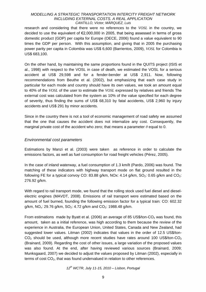
The correct way to establish the value of statistical life (VOSL) for Colombia involves the

development of a specific study to determine the willingness to pay for reducing the risk of

accidents. However, since implementation of the study was beyond the scope of this




9

research and considering that there were no references to the VOSL in the country, we

decided to use the equivalent of €2,000,000 in 2005, that being assessed in terms of gross

domestic product (GDP) per capita for Europe (OECE, 2006) found a value equivalent to 90

times the GDP per person. With this assumption, and giving that in 2005 the purchasing

power parity per capita in Colombia was US$ 6,600 (Barrientos, 2009), VOSL for Colombia is

US$ 683,100.

On the other hand, by maintaining the same proportions found in the QUITS project (ISIS et

al., 1998) with respect to the VOSL in case of death, we estimated the VOSL for a serious

accident at US$ 29,598 and for a fender-bender at US$ 2,911. Now, following

recommendations from Beuthe et al. (2002), but emphasizing that each case study in

particular for each mode and country should have its own values, we took an amount equal

to 40% of the VOSL of the user to estimate the VOSL expressed by relatives and friends The

external cost was calculated from the system as 10% of the value specified for each degree

of severity, thus finding the sums of US$ 68,310 by fatal accidents, US$ 2,960 by injury

accidents and US$ 291 by minor accidents.

Since in the country there is not a tool of economic management of road safety we assumed

that the one that causes the accident does not internalize any cost. Consequently, the

marginal private cost of the accident who zero; that means a parameter θ equal to 0.

Environmental cost parameters

Estimations by Manzi et al. (2003) were taken as reference in order to calculate the

emissions factors, as well as fuel consumption for road freight vehicles (Pérez, 2005).

In the case of inland waterway, a fuel consumption of 1.3 km/lt (Pardo, 2006) was found. The

matching of these indicators with highway transport mode on flat ground resulted in the

following FE for a typical convoy CO: 83.88 g/km, NOx: 4.14 g/km, SO2: 0.65 g/km and CO2:

276.92 g/km.

With regard to rail transport mode, we found that the rolling stock used fuel diesel and diesel-

electric engines (MAVDT, 2008). Emissions of rail transport were estimated based on the

amount of fuel burned, founding the following emission factor for a typical train: CO: 602.32

g/km, NOx: 29.76 g/km, SO2: 4.72 g/km and CO2: 1988.48 g/km.

From estimations made by Byatt et al. (2006) an average of 85 US$/ton-CO2 was found, this

amount, taken as a initial reference, was high according to them because the review of the

experience in Australia, the European Union, United States, Canada and New Zealand, had

suggested lower values. Litman (2002) indicates that values in the order of 12.5 US$/ton-

CO2 should be used, although more recent studies have rates around 100 US$/ton-CO2

(Brainard, 2009). Regarding the cost of other issues, a large variation of the proposed values

was also found. At the end, after having reviewed various sources (Brainard, 2009;

Munksgaard, 2007) we decided to adjust the values proposed by Litman (2002), especially in

terms of cost CO2, that was found undervalued in relation to other references.




10

Parameters of the cost of infrastructure

The calculation of the costs associated with road infrastructure taken as a basis for annual

maintenance costs per mile shown in the official document CONPES 3085 (DNP, 2000),

finds an average routine maintenance cost equal to 2.06×103 US$/km and periodic

maintenance cost equal to 19.3×103 US$/ km. Intending to use a single marginal cost

parameter for the entire network of road transport, an average speed was calculated and

after applying the relationship proposed by Ozbay et al. (2007), a value of 0.01383

US$/pce/km was found, assuming that the other vehicles that use the infrastructure does not

cause damage.

Following the same scheme of calculation, the rail transport mode value of 0.1115 US$/train

type/km was found, which under operating conditions (Arias et al., 2007) is internalized by

existing shareholders, which carried its own risk under the investments to expand and

maintain the rail network concession that is in operation.

Moreover, we found that major maintenance projects in major river corridors, are aimed at

controlling floods and sedimentation, maintenance of airworthiness and expansion of port

infrastructure. Dredging, which allow you to retrieve the seaworthiness of the rivers, is not

properly related to the use of infrastructure by the river boats, but is derived from transport

and disposal of sediments that the fluvial dynamics causes. For this reason, we considered

that the marginal damage caused to the infrastructure of a convoy-type effect can be

dismissed without incur higher pricing errors, so for inland waterway transport, a null

incremental cost of maintenance was assumed.

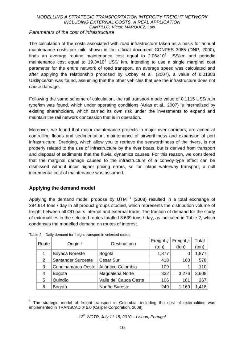
Applying the demand model

Applying the demand model propose by UTMT1 (2008) resulted in a total exchange of

384.914 tons / day in all product groups studied, which represents the distribution volume of

freight between all OD pairs internal and external trade. The fraction of demand for the study

of externalities in the selected routes totalled 8.639 tons / day, as indicated in Table 2, which

condenses the modelled demand on routes of interest.

Table 2 – Daily demand for freight transport in selected routes

Route Origin i Destination j Freight ij

(ton)

Freight ji

(ton)

Total

(ton)

1 Boyacá Noreste Bogotá 1,877 0 1,877

2 Santander Suroeste Cesar Sur 418 160 578

3 Cundinamarca Oeste Atlántico Colombia 109 1 110

4 Bogotá Magdalena Norte 332 3,276 3,608

5 Quindío Valle del Cauca Oeste 106 161 267

6 Bogotá Nariño Sureste 249 1,169 1,418

1 The strategic model of freight transport in Colombia, including the cost of externalities was

implemented in TRANSCAD ® 5.0 (Caliper Corporation, 2009)




11

7 Antioquia Metro Norte de Santander Sur 478 303 781

Although OD pairs given in Table 2 relate only to internal areas, the calculation of the

tonnage moved in certain routes included a portion of the volume of tons of foreign trade; as

an example, in the case of Route 6 was added the tonnage being mobilized between Bogota

and Ecuador, and Route 7 was added the weight of foreign trade goods between the

Metropolitan Area of Medellin and Venezuela. A similar treatment was given to routes 3 and

5 which contain respectively the foreign trade demand mobilized through the ports of

Barranquilla and Buenaventura.

Travel times in the equilibrium condition (Table 3) do not differ significantly with respect to

the time of reference, especially for water transport due to the broad capabilities of the links.

Particularly, the modelled travel times are not comparable with the actual operation times in

this model, because it does not consider spent time in ports.

Table 3 – Travel times by mode of transport on the analyzed routes

Route Description Time (hours)

Roadway River Rail

1 Boyacá Noreste - Bogotá 5.12 11.53

2 Santander Suroeste - Cesar Sur 4.36 15.00 15.87

3 Cundinamarca Oeste - Atlántico Colombia 12.52 52.81

4 Bogotá - Magdalena Norte 14.95 41.60

5 Quindío - Valle del Cauca Oeste 5.22 9.34

6 Bogotá - Nariño Sureste 22.14

7 Antioquia Metro - Norte de Santander Sur 16.97

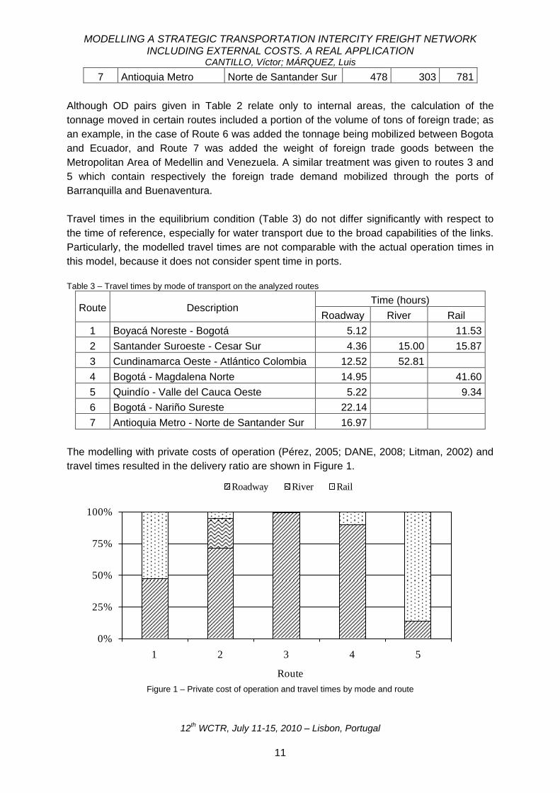
The modelling with private costs of operation (Pérez, 2005; DANE, 2008; Litman, 2002) and

travel times resulted in the delivery ratio are shown in Figure 1.

0%

25%

50%

75%

100%

1 2 3 4 5

Route

Roadway River Rail

Figure 1 – Private cost of operation and travel times by mode and route




12

We found that share market of inland waterway transport is very low because it is heavily

penalized for operating with travel times significantly greater than those of its competitors.

Internal costs

It were calculated the internal costs on each of the routes and transport modes initially using

a VOT ratio equal to 0,11 US$/hour/ton (Fowkes et al., 1989; Ministerio de Transporte,

2007a; DANE, 2008), affected by the average number of tons mobilized by each transport

unit equivalent.

In the case of road transport, we found that, on average, the cost of time is equal to 5% of

total domestic cost considered (Table 4), which partly explains the predominance of this

mode of transport in the country, given the freight opportunity costs, as well as its greater

reliability in delivery times, therefore becoming more attractive.

Table 4 – Domestic costs of roadway

Route Description Internal cost (US$/pce)

Time Operation Total

1 Boyacá Noreste - Bogotá 2.96 50.05 53.01

2 Santander Suroeste - Cesar Sur 2.52 51.34 53.86

3 Cundinamarca Oeste - Atlántico Colombia 7.23 145.13 152.36

4 Bogotá - Magdalena Norte 8.63 170.65 179.28

5 Quindío - Valle del Cauca Oeste 3.02 55.59 58.61

6 Bogotá - Nariño Sureste 1.28 201.42 202.69

7 Antioquia Metro - Norte de Santander Sur 9.80 154.52 164.32

In contrast, as shown in Table 5, in inland waterway transport the domestic cost associated

with time in a convoy rate is around 60% of the total domestic cost, and this may be reason

why this alternative is mainly used in the movement of goods with low opportunity costs.

Table 5 – Internal costs of inland transport

Route Description Internal cost (US$/convoy)


2 Santander Suroeste - Cesar Sur 1,323.2 765.1 2,088.3

3 Cundinamarca Oeste - Atlántico Colombia 4,657.8 2,693.3 7,351.1

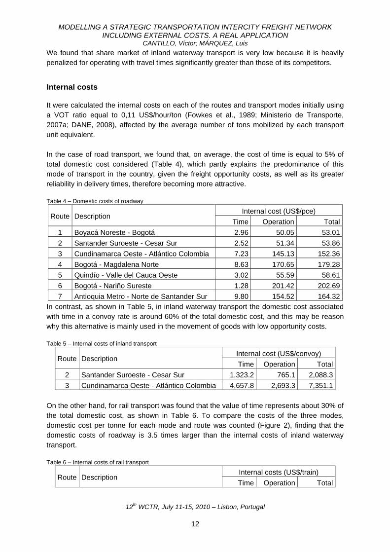
On the other hand, for rail transport was found that the value of time represents about 30% of

the total domestic cost, as shown in Table 6. To compare the costs of the three modes,

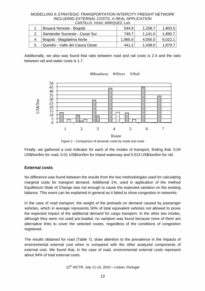
domestic cost per tonne for each mode and route was counted (Figure 2), finding that the

domestic costs of roadway is 3.5 times larger than the internal costs of inland waterway

transport.

Table 6 – Internal costs of rail transport

Route Description Internal costs (US$/train)





13

1 Boyacá Noreste - Bogotá 544.8 1,258.7 1,803.5

2 Santander Suroeste - Cesar Sur 749.7 1,141.0 1,890.7

4 Bogotá - Magdalena Norte 1,965.6 4,056.5 6,022.1

5 Quindío - Valle del Cauca Oeste 441.2 1,438.6 1,879.7

Additionally, we also was found that ratio between road and rail costs is 2.4 and the ratio

between rail and water costs is 1.7.

05

101520253035404550

1 2 3 4 5 6 7

US

$/T

on

Route

Roadway River Rail

Figure 2 – Comparison of domestic costs by mode and route

Finally, we gathered a cost indicator for each of the modes of transport, finding that: 0.04

US$/ton/km for road, 0.01 US$/ton/km for inland waterway and 0.013 US$/ton/km for rail.

External costs

No difference was found between the results from the two methodologies used for calculating

marginal costs for transport demand. Additional 1%, used in application of the method

Equilibrium State of Change was not enough to cause the expected variation on the existing

balance. This event can be explained in general as it failed to show congestion in networks.

In the case of road transport, the weight of the preloads on demand caused by passenger

vehicles, which in average represents 50% of total equivalent vehicles not allowed to prove

the expected impact of the additional demand for cargo transport. In the other two modes,

although they were not used pre-loaded, no variation was found because none of them are

alternative links to cover the selected routes, regardless of the conditions of congestion

registered.

The results obtained for road (Table 7), draw attention to the prevalence in the impacts of

environmental external cost when is compared with the other analyzed components of

external cost. We found that, in the case of road, environmental external costs represent

about 94% of total external costs.




14

Table 7 – External costs for road transport

Route External cost (US$/pce)

Congestion Accidents Environmental Total

1 1.1660 0.1490 18.8425 20.1575

2 0.9925 0.1750 17.5260 18.6935

3 2.8475 0.4830 49.1275 52.4580

4 3.4010 0.5575 61.0195 64.9780

5 1.1885 0.1780 23.1875 24.5540

6 5.0365 0.5130 76.2540 81.8035

7 3.8610 0.4100 59.3005 63.5715

We also found that, for road transport, cost of the accidents is the minor component since it

fails to represent even 1% on the total external cost, which is reasonable since accidents are

a phenomenon greater importance in urban areas. Table 8 summarizes the external costs of

inland waterway transport. It does not register external costs associated with congestion and

the social costs of accidents are irrelevant, the whole burden of indirect costs is on the

environmental impact assessment, represented by the costs of emissions.

Table 8 – External costs of inland waterway transport

Route External cost (US$/convoy)

Congestion Accident Environmental Total

2 0 0,000 22.6865 22.6895

3 0 0,0003 79.8610 79.8613

In the rail transport mode (Table 9) we found that the external environmental cost is the most

important of all, representing just over 87% of the total external costs, followed by the

external cost of congestion to 12%. This latter cost is particularly high and perceived

explained. First, by the way the links were penalized representing the passage through the

seasons, and second, by the low capacity of railway links that feeds the BPR function.

Table 9 – External costs of rail transport

Route External cost (US$/train)

Congestion Accident Environmental Total

1 25.12 0.01 192.55 217.68

2 34.58 0.01 174.54 209.12

3 90.64 0.02 620.53 711.19

4 20.34 0.01 220.06 240.41

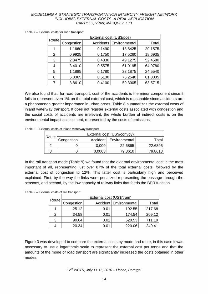
Figure 3 was developed to compare the external costs by mode and route, in this case it was

necessary to use a logarithmic scale to represent the external cost per tonne and that the

amounts of the mode of road transport are significantly increased the costs obtained in other

modes.




15

0,01

0,10

1,00

10,00

1 2 3 4 5 6 7

US

$/T

on

Route

Roadway River Rail

Figure 3 – Comparison of external costs by mode and route

A comparison of external costs between different transport modes resulted in a ratio of 1 to

110 of the external costs of road with regard to inland waterway transport, and 1 to 8 of road

with respect to rail transport mode. A ratio of 1 to 17 was obtained, in the only comparable

route between modes of inland waterways and rail.

Finally, an average rate of external costs for each mode of transport was obtained, finding

that: 0.014 US$ / ton / km for road, 0.0001 US$ / ton / km in inland waterway transport and

0.0016 US$ / ton / km in the case of rail transport.

So, in the mode of road transport external costs are equivalent to 37% of domestic costs

valued, in the rail transport mode they reach an amount equivalent to 12% and inland

waterway transport they represent only something higher than 1%.

Sensitivity of external costs to change the VOT

The calculation of TMC was evaluated with three VOT, in order to incorporate the effect of

three different product types into analysis: one with a low opportunity cost, one with medium

and opportunity cost another with high opportunity cost.

Similar to other transport modes , the results for road transport mode (Table 10) were not

encouraging due mainly to the specification of demand model (UTMT, 2008) which

envisaged a single modal model whose variables are the perceived monetary: cost and

travel time. That is, this model alone could not reproduce directly changes in modal split due

to changes in the VOT. To do so, changing the partition model parameters in response to the

mobilization of goods with varying degrees of opportunity cost, would be required; which was

not included in the scope of the research.

Table 10 – External costs of road transport mode with variations of VOT

Route Description External cost (US$/ton)




16

Low Medium High

1 Boyacá Noreste - Bogotá 3,514 3,665 3,816

2 Santander Suroeste - Cesar Sur 3,270 3,399 3,527

3 Cundinamarca Oeste - Atlántico Colombia 9,168 9,538 9,907

4 Bogotá - Magdalena Norte 11,373 11,814 12,255

5 Quindío - Valle del Cauca Oeste 4,310 4,465 4,618

6 Bogotá - Nariño Sureste 14,220 14,874 15,526

7 Antioquia Metro - Norte de Santander Sur 11,057 11,559 12,059

Simulation of internalisation

Initially, 50% internalization of external costs of environmental impacts of road transport

mode was simulated by introducing a proportional increase in operating costs per route, as

shown in Table 11.

Table 11 – Simulated operating costs for highway transport

Route Description Cost simulation (US$/pce)


1 Boyacá Noreste - Bogotá 2,960 59,468 62,428

2 Santander Suroeste - Cesar Sur 2,519 60,103 62,622

3 Cundinamarca Oeste - Atlántico Colombia 7,229 169,693 176,922

4 Bogotá - Magdalena Norte 8,634 201,159 209,792

5 Quindío - Valle del Cauca Oeste 3,018 67,183 70,201

6 Bogotá - Nariño Sureste 12,785 239,543 252,328

7 Antioquia Metro - Norte de Santander Sur 9,801 184,173 193,974

This simulation represented the increased costs of operating the highway transport mode at

rates ranging from 16% to 20% depending on the characteristics of each route, finding the

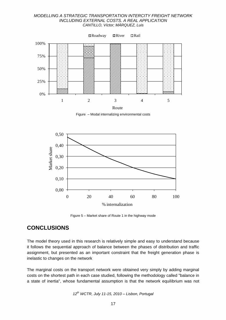
new modal split shown in Figure 4.

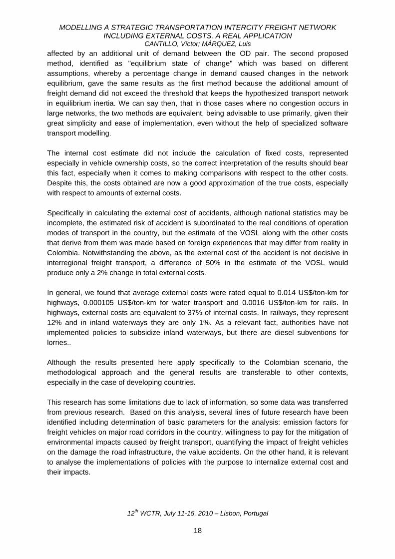
Many other experiments can be simulated with the model. It proved to be very sensitive to

changes in the perceived costs incurred, as shown in Figure 5 which represents changes in

road market share for route 1, assuming different levels of internalization of environmental

costs.




17

0%

25%

50%

75%

100%

1 2 3 4 5

Route

Roadway River Rail

Figure – Modal internalizing environmental costs

0,00

0,10

0,20

0,30

0,40

0,50

0 20 40 60 80 100

Mar

ket

shar

e

% internalization

Figure 5 – Market share of Route 1 in the highway mode

CONCLUSIONS

The model theory used in this research is relatively simple and easy to understand because

it follows the sequential approach of balance between the phases of distribution and traffic

assignment, but presented as an important constraint that the freight generation phase is

inelastic to changes on the network

The marginal costs on the transport network were obtained very simply by adding marginal

costs on the shortest path in each case studied, following the methodology called "balance in

a state of inertia", whose fundamental assumption is that the network equilibrium was not




18

affected by an additional unit of demand between the OD pair. The second proposed

method, identified as "equilibrium state of change" which was based on different

assumptions, whereby a percentage change in demand caused changes in the network

equilibrium, gave the same results as the first method because the additional amount of

freight demand did not exceed the threshold that keeps the hypothesized transport network

in equilibrium inertia. We can say then, that in those cases where no congestion occurs in

large networks, the two methods are equivalent, being advisable to use primarily, given their

great simplicity and ease of implementation, even without the help of specialized software

transport modelling.

The internal cost estimate did not include the calculation of fixed costs, represented

especially in vehicle ownership costs, so the correct interpretation of the results should bear

this fact, especially when it comes to making comparisons with respect to the other costs.

Despite this, the costs obtained are now a good approximation of the true costs, especially

with respect to amounts of external costs.

Specifically in calculating the external cost of accidents, although national statistics may be

incomplete, the estimated risk of accident is subordinated to the real conditions of operation

modes of transport in the country, but the estimate of the VOSL along with the other costs

that derive from them was made based on foreign experiences that may differ from reality in

Colombia. Notwithstanding the above, as the external cost of the accident is not decisive in

interregional freight transport, a difference of 50% in the estimate of the VOSL would

produce only a 2% change in total external costs.

In general, we found that average external costs were rated equal to 0.014 US$/ton-km for

highways, 0.000105 US$/ton-km for water transport and 0.0016 US$/ton-km for rails. In

highways, external costs are equivalent to 37% of internal costs. In railways, they represent

12% and in inland waterways they are only 1%. As a relevant fact, authorities have not

implemented policies to subsidize inland waterways, but there are diesel subventions for

lorries..

Although the results presented here apply specifically to the Colombian scenario, the

methodological approach and the general results are transferable to other contexts,

especially in the case of developing countries.

This research has some limitations due to lack of information, so some data was transferred

from previous research. Based on this analysis, several lines of future research have been

identified including determination of basic parameters for the analysis: emission factors for

freight vehicles on major road corridors in the country, willingness to pay for the mitigation of

environmental impacts caused by freight transport, quantifying the impact of freight vehicles

on the damage the road infrastructure, the value accidents. On the other hand, it is relevant

to analyse the implementations of policies with the purpose to internalize external cost and

their impacts.




19

REFERENCES

Arias, J. A. et al. (2007). Desarrollo de las concesiones férreas en Colombia. Contraloría

General de la República. Sector infraestructura física y telecomunicaciones, comercio

exterior y desarrollo regional. Bogotá, noviembre 19 de 2007. 67 p.

Barrientos, M. (2009). Colombia – Producto Interno Bruto (PIB) per capita (US$).

[Documento en línea]: http://www.indexmundi.com/g/g.aspx?c=co&v=67&l=es

[Consulta: 19-5-2009]. 2009.

Beuthe, M. et al. (2002). External costs of the Belgian interurban freight traffic: a network

analysis of their internalisation. Transportation Research Part D 7 (2002) 285–301.

www.elsevier.com

Bickel P. et al. (2006). Introducing Environmental Externalities into Transport Pricing:

Measurement and Implications. Transport Reviews, Vol. 26, No. 4, 389–415, July

2006.

Brainard, J. et al. (2009). ―The social value of carbon sequestered in Great Britain's

woodlands‖. Ecological Economics, Volume 68, Issue 4, 15 February 2009, Pages

1257-1267. 2009.

Branston, D. (1976) Link Capacity Functions: A Review. Transportation Research 10, 223-

236.

Byatt, I. et al. (2006). ―The Stern Review: A Dual Critique. Part II: Economics Aspects‖. World

Economics 7(3): 199-229. 2006.

Caliper Corporation (2009). Travel Demand Modeling with TransCAD 5.0. Newton,

Massachusetts.

Davidson, K. B. (1966). A flow travel time relationship for use in transportation planning.

Australian Road Research Board 3, 183-194.

Departamento Administrativo Nacional de Estadística (DANE, 2008). Variación del índice de

precios al consumidor IPC en Colombia 1993 – 2008 [On line].

http://www.dane.gov.co/files/investigaciones/ipc/dic08/IPC_Variacion.xls [16-3-2009].

Departamento Nacional de Planeación (DNP, 2000). Documento CONPES 3085. Plan de

expansión de la red nacional de carreteras. DNP: UINFE-DITRAN, Ministerio de

Transporte, Instituto Nacional de Vías. Versión aprobada

EEA (2003). EMEP/CORINAIR Emissions Inventory Guidebook. 3rd edition. September 2003

update. Technical report Nº 30.

Federal Highway Administration (FHWA, 2000). Highway cost responsibility. [Available on

line]: <http://www.fhwa.dot.gov/policy/hcas/final/five.htm>. [Reference: 11-11-2008]

Fondo de Prevención Vial (2005). Informe de Accidentalidad 2005. Capítulo 1.

www.fonprevial.org.co. 2005.

Fowkes, A. S. et al. (1989). Valuing the attributes of freight transport quality: Results of the

stated preference survey. ITS working paper 276.University of Leeds, Institute for

Transport Studies. Leeds, Yorkshire, UK

Guo, Shwu-Ping (2007) Internalization of Transportation External Costs: Impact Analysis of

Logistics Company Mode and Route Choices, Transportation Planning and

Technology, 30: 2, 147 — 165

HOLGUÍN-VERAS, J. y THORSON E. (2003). Practical Implications of Modeling Commercial

Vehicle Empty Trip. Transportation Research Record 1833, 87 - 90.




20

INFRAS (2004). External cost of transport, Update Study. Final Report, Zurich/Karlsruhe,

October 2004.

ISIS et al. (1998). QUITS, Quality Indicators for Transport Systems. Final Report For

Publication. Contract n°: ST-96-SC-115. Project funded in part by THE EUROPEAN

COMMISSION – DGVII under the Transport RTD Programme of the 4th Framework

Programme. Rome, April 1998.

Lindberg, G. (2002). Deliverable 9: Accident Cost Case Studies, Case Study 8d: External

Accident Cost of Heavy Goods Vehicles. (UNIfication of accounts and marginal costs

for Transport Efficiency) Deliverable 9. Funded by 5th Framework RTD Programme.

ITS.

Litman, T. (2002). Transportation Cost Analysis: Techniques, Estimates and Implications.

Victoria Transport Policy Institute. June 2002.

Maibach, M. (2008). Handbook on estimation of external costs in the transport sector.

Produced within the study Internalisation Measures and Policies for All external Cost

of Transport (IMPACT).

Manzi, V. et al. (2003). ―Estimación de los factores de emisión de las fuentes móviles en la

ciudad de Bogotá‖. Revista de Ingeniería Universidad de los Andes. Revista 18,

Noviembre 2003, 18 – 25. 2003.

Márquez, L. (2008). Informe de Zonificación. Investigación para ―Desarrollar y poner en

funcionamiento los modelos de demanda y de oferta de transporte que permitan

proponer opciones en materia de infraestructura para aumentar la competitividad de

los productos colombianos‖. Unión Temporal Modelación de Transporte, Bogotá.

Márquez, L. (2008). Modelo de oferta de transporte para Colombia: Calibración y

Asignación. Unión Temporal Modelación de Transporte, Bogotá. 2008.

Ministerio de Ambiente, Vivienda y Desarrollo Territorial (MAVDT, 2008). Manual de

inventario de fuentes difusas. Available on line: www1.minambiente.gov.co/prensa/

banner_home/proyectos_en_tramite/inventario_emisiones/4_fuentesfijasdifusas.doc.

2008

Ministerio de Transporte (2006). Metodologías tarifarias del transporte fluvial en Colombia:

Análisis conceptual. Oficina de Regulación Económica, Bogotá, Mayo de 2006

Ministerio de Transporte (2007). Anuario Estadístico de Transporte 2006. Oficina de

Planeación. Grupo de Planeación sectorial.

Munksgaard, J. et al. (2007). ―An environmental performance index for products reflecting

damage costs‖. Ecological Economics, Volume 64, Issue 1, 15 October 2007, p 119-

130.

National Research Council (2000). Transportation Research Board. 2000 Highway Capacity

Manual. Washington, D.C.: Transportation Research Board National Research

Council.

Organisation for Economic Co-Operation and Development (OECD, 2006). Table 2.

Breakdown of GDP per capita in its components, 2005. [Available on line]:

http://www.oecd.org/dataoecd/ 30/40/29867116.xls. 2006

Ozbay, K., B. Bartin, O. Yanmaz-Tuzel and J. Berechman (2007). Alternative methods for

estimating full marginal costs of highway transportation. Transportation Research

Part A 41 (2007) 768-786.




21

Pardo, M. et al. (2006). ―Método de medición de combustible en una embarcación fluvial‖.

Revista Ingeniería y Ciencia, Volumen 2, número 3, páginas 5-27, marzo de 2006.

Pérez, G. J. (2005). La infraestructura del transporte vial y la movilización de carga en

Colombia. Documentos de trabajo sobre economía regional No. 64, Octubre 2005.

Banco de la República. 1692-3715. 70 p.

Rizzi, L.I. (2005). Diseño de instrumentos económicos para la internalización de

externalidades de accidentes de tránsito. Cuadernos de Economía, Vol. 42

(Noviembre) Pontificia Universidad Católica de Chile.

Spiess, H. (1990) Conical Volume-Delay Functions. Transportation Science 24, 153-158.

Unión Temporal Modelación del Transporte (UTMT, 2008). Informe Final de la Investigación

para ―Desarrollar y poner en funcionamiento los modelos de demanda y de oferta de

transporte que permitan proponer opciones en materia de infraestructura para

aumentar la competitividad de los productos colombianos‖.

modelling a strategic transport intercity freight …a relevant issue for freight transport system...

Documents