~3FI~LE COPY

Modeling the Transport ofHeavy Metals in Soils

0) HM. Selim, M.C. Amacher and KX Iskandar September 1990

BEST

AVAILABLE COPY

0 Rser oi Colum

_____ _____ ____ELECTE

NOV28 1M9

For conversion of Sl metric units to U.S./British customary unitsof measurement consult ASTM Standard E380, Metric PracticeGuide, published by the American Society for Testing andMaterials, 1916 Race St., Philadelphia, Pa. 19103.

Cover: The experimental design of the transport experiments.

A PC-compatible disketteof the computer models isavailable upon requestfrom the authors

Monograph 90-2

U.S. Army Corpsof EngineersCold Regions Research &Engineering Laboratory

Modeling the Transport ofHeavy Metals in SoilsH.M. Selim, M.C. Amacher and I.K. Iskandar September 1990

Prepared for

OFFICE OF THE CHIEF OF ENGINEERS

Approved for public release; distribution is unlimited. 90 11 27 019

PREFACE

H.M. Selim and M.C. Amacher are Professor of soil physics and Associate Professor of soilchemistry, respectively, at Louisiana State University, Baton Rouge, Louisiana. I.K. Iskandar isChief of the Geochemical Branch, Research Division, Cold Regions Research and EngineeringLaboratory (CRREL), Hanover, New Hampshire. Dr, Amacher is now with the Forestry SciencesLaboratory, Intermountain Research Station, USDA Forest Service, Logan, Utah. This work wasconducted under Hatch projects 1898 and 2469 of the Louisiana Agricultural Experiment Stationand was funded in part by CRREL under research program element 6.11 .02A, Project No.4A 161102AT24, Research in Snow. Ice, and Frozen Ground; Task SS, Work Unit 020, Transport

of Chentical Species in Soils.The authors wish to acknowledge B. Davidoff, S. Louque, and B. Buchter for their assistance

during the course of this work. Special thanks to M. Bergstad, technical editor, CRREL, for herefforts in editing and overall organization of the manuscript. Her contribution not only enhancedthe quality but is also a tremendous improvement of the presentation of the work included in themonograph.

The contents of this report are not to be used for advertising or promotional purposes. Citationof brand names does not constitute an official endorsement or approval of the use of suchcommercial products.

Acoession For

NTIS GRA&IDTIC

TAB

Unannounced QJustification

ByDistribution/

Avallability Code1Svail and/or

Dist Spec 181

CONTENTSPage

Preface ............................................................................................. iiNomenclature..................................................................................... vChapter 1. Introduction............................................................................1

Scope of the monograph........................................................................ 2Equilibrium retention models.................................................................. 2Kinetic models .................................................................................. 4

Chapter 2. Heavy Metals Retention in Soils: A Simplified Approach ......................... 7A simplified approach .......................................................................... 7Soils and nothods............................................................................... 8

Soils ........................................................................................ 8Metals ...................................................................................... 9Experimental procedure..................................................................... 9

Retention characteristics ....................................................................... 9Chapter 3. A Kinetic Multireaction, Approach ................................................... J 6

Formulation of models ......................................................................... 16Multireaction model......................................................................... 16Multi reaction and transport model ......................................................... 17Initial and boundary conditions............................................................. 19

Sensitivity analysis............................................................................. 22MRM computer program ...................................................................... 26MRTM computer program..................................................................... 28

Chapter 4. Describing Cr(VI) and Cd Retention in Soils Using the Multireaction Model ...30The model..................................................................................... 30Experimental methods and analysis ........................................................... 31

Soils........................................................................................ 31Reagents .................................................................................... 32Procedure.................................................................................... 32Data analysis ................................................................................ 32

Model validation ............................................................................... 33Model variations............................................................... 33Cr and Cd retention kinetics ................................................................ 34Release of Cr and Cd........................................................................ 39Sensitivity analysis.......................................................................... 42Mechanism consistent with model ......................................................... 42

Chapter 5. Retention Kinetics of Mercury in Soils Using the Multireaction Model .......... 45Experimental and data analysis................................................................ 45

Soils........................................................................................ 45Reagents .................................................................................... 46Procedure................................................................................... 46Data analysis ................................................................................ 47

Model evaluation ........................................................... ................... 47Chapter 6. Predicting CR(VI) Transport Based on the Multireaction and Transport Model .. 52

The model..................................................................................... 52Experimental methods ......................................................................... 52Evaluation of the MRTM ...................................................................... 54

iii

PageChapter 7. A Second-Order Two-Site Retention and Transport M odel ................................. 60

M odel formulation ............................................................................................................. 60Second-order kinetics ................................................................................................... 60Transport model ............................................................................................................ 62

Sensitivity analysis ............................................................................................................ 64Reaction kinetics ......................................................................................................... 64Transport ....................................................................................................................... 66

SOTS computer program .................................................................................................. 70Chapter 8. A Second-Order Mobile-Immobile Retention and Transport Model .................. 72

Model formulation ............................................................................................................. 72Initial and boundary conditions ................................................................................... 75Numerical solutions .................................................................................................... 75

Sensitivity analysis ............................................................................................................ 76SOM IM computer program .............................................................................................. 79

Chapter 9. A Second-Order Retention Approach: Validation .............................................. 82Experimental ...................................................................................................................... 82Kinetics .............................................................................................................................. 83SOTS model validation ..................................................................................................... 89SOM IM validation ............................................................................................................. 91

References .............................................................................................................................. 94Appendix A: M RM computer program listing ....................................................................... 101Appendix B: M RTM computer program listing .................................................................. IIlAppendix C: SOTS model computer program listing ............................................................. 125Appendix D: SOM IM computer program listing .................................................................... 139Abstract ................................................................................................................................... 157

ILLUSTRATIONS

Figure2- I. Retention isotherm s for cadmium on selected soils ..................................................... I12-2. Retention isotherm s for chromium on selected soils ................................................... 112-3. Retention isotherms for selected cation species on Alligator soil ............................... 132-4. Retention isotherms for selected anion species on Alligator soil .............................. 132-5. Comparison chart of soils and elements for Freundlich parameter b .......................... 142-6. Correlation between soil pH and b values .................................................................. 143-1. Schematic diagram of the multireaction retention model .......................................... 163-2. Breakthrough curves for several Kd values where b = 0.5 and k = k2 .. = k = 0. 22S 233-3. Breakthrough curves for several b values where b 1.0 and k, = k2 .. = k ... 233-4. Breakthrough curves for several b values where b > 1.0 and kt = k ... = ks = 0. 23

3-5. Breakthrough curves for several values of rate coefficients (k, and k2) ................ 243-6. Breakthrough curves for several b values where k, and k2 and kl/k 2 remain invariant

and k3 = k4 = ... =k = 0 ....................................................................................... 243-7. Breakthrough curves for several values of nonlinear parameter n associated with s,

where k3 = k4 = ... = ks =0 .................................................................................. 243-8. Breakthrough curves for several values of irreversible rate coefficient k (where b = I

andk 3 =k 4 = .... k!=0 ....................................................................................... 253-9. Breakthrough curves for several values of irreversible rate coefficient k, (where

b = 0.5 and k3 = k4 =. .. s = ) .......................................................................... 253-10. Breakthrough curves for several values of rate coefficients k5 and k6 (where k3 =

k4=ks =0) ................................................................................................................ 26

iv

Figure Page3-1 I. Breakthrough curves for several values of rate coefficient k5 (where k3 = k = k6 =

k = 0 ) .................................................................................................................... 264-1. Prediction of experimental data for Cr(VI) retention by Windsor soil using six model

variatio ns ............................................................................................................... 344-2. Prediction of experimental data for Cr(VI) retention by seven soils .......................... 384-3. Prediction of experimental data for Cd retention by four soils ................................... 384-4. Prediction of experimental data for Cr(VI) retention by Windsor soil ....................... 384-5. Prediction of experimental data for Cd retention by Windsor soil ............................. 394-6. MRM predictions of the time-dependent amounts of Cr retained by three phases of a

W indsor soil ....................................................................................................... 404-7. Time-dependent release of Cr and Cd from a Windsor soil at several initial concentra-

tions of retained m etal .......................................................................................... 404-8. Cumulative amounts of Cr and Cd released from several soils as a function of the

initial amount of metal retained by the soils at the start of metal release ............. 414-9. Effect of model variations on model simulations ..................................................... 42

4-10. Effect of reaction order on model simulations .......................................................... 434-1I. Effect of rate coefficients on model simulations ....................................................... 43

5-i. Mercuric chloride retention isotherms for Cecil soil at each sampling time from 2 to336 hr .................................................................................................................... 4 7

5-2. Time-dependent HIgCl, retention by Cecil soil .......................................................... 495-3. Time-dependent HgCl.retention by Norwood soil ..................................................... 495-4. Time-dependent HgCI., retention by Olivier soil ........................................................ 495-5. Time-dependent HgCI 2 retention by Sharkey soil ..................................................... 495-6. Time-dependent HgCI, retention by Windsor soil ..................................................... 495-7. Time-dependent mercury release from Cecil soil ..................................................... 505-8. Cumulative mercury release as a function of retained mercury ................................. 506-1. Chloride-36 and tritium breakthrough curves (BTCs) for Cecil and Windsor soils .... 546-2. Measured and predicted BTCs for Cr(VI) in Calciorthid soil (column no. 101) ........... 556-3. Measured and predicted BTCs for Cr(VI) in Norwood soil (v = 0.14 cm h ic .......... 566-4. Measured and predicted BTCs for Cr(VI) in Norwood soil (v = 1.04 cm hr - .......... 566-5. Measured and predicted BTCs for Cr(VI) in Webster soil ......................................... 576-6. Measured and predicted BTCs for Cr(VI) in Olivier soil ............................................ 576-7. Measured and predicted BTCs for Cr(VI) in Cecil soil using the three-parameter

m od el .................................................................................................................... 586-8. Measured and predicted BTCs for Cr(VI) in Cecil soil using the five-parameter

m od el .................................................................................................................... 586-9. Measured and predicted BTCs for Cr(VI) in Windsor soil ........................................ 587-1. Effect ofratecoefficients on sorption isotherms using thesecond-order kinetic model 647-2. Effect of time of retention on sorption isotherms using the second-order kinetic model 657-3. Effect of total amount of sites on the shape of sorption isotherms using the second-

order kinetic m odel .............................................................................................. 657-4. Effluent concentration distributions for different initial concentrations using the

second-order two-site model .............................................................................. 667-5. Effluent concentration distributions for different sT values using the SOTS model .... 667-6. Effluent concentration distributions for different flux values using the SOTS model. 677-7. Effluent concentration distributions for values of the irreversible rate coefficient

using the SO T S m odel ......................................................................................... 687-8. Effluent concentration distributions for different values of parameter Q of the SOTS

m od e l .................................................................................................................... 68

v

Figure Page7-9. Effluent concentration distributions for different values of rate coefficients using the

SO T S m odel ........................................................................................................ 697-10. Effluent concentration distributions for different values of the fraction of sites F

using the SO TS m odel ......................................................................................... 698-I. ELa-uent concentration distributions for different values of K1 and K2 using the

SO M iM ................................................................................................................. 778-2. Effluent concentration distributions for different values of parameter o0 using the

SO M IM ................................................................................................................. 778-3. Effluent concentration distributions for different values of the dimensionless mass

transfer parameter ox of the SOMIM ................................................................... 788-4. Effluent concentration distributions for different values of parameter 12 of the

SO M IM ................................................................................................................. 788-5. Effluent concentration distributions for different values of the fraction of active sites

f m of the SO M IM ................................................................................................ 799-I. Chromium (VI) sorption isotherms for Cecil, Windsor, and Olivier soils after 14

days of reaction ................................................................................................... 849-2. Concentration of Cr vs time for a range of initial concentrations for Olivier soil ....... 879-3. Concentration of Cr vs time for a range of initial concentrations for Windsor soil ..... 879-4. Concentration of Cr vs time for a range of initial concentrations for Cecil soil .......... 879-5. Effluent concentration distributions for Cr predicted using the SOTS model with the

batch rate coefficients indicated .......................................................................... 909-6. Effluent concentration distributions for Cr predicted using the SOMIM with the

batch rate coefficients indicated .......................................................................... 92

TABLES

Tablel- I. Selected equilibrium and kinetic type models for solute retention in soils .................. 42- 1. Taxonomic classification and selected soil properties ................................................. 82-2. Concentrations and forms of elements ........................................................................ 92-3. Freundlich model parameters for I I soils and 15 elements ........................................ 102-4. Simple correlation coefficients for selected soil properties and Freundlich parameters 123- 1. List of input parameters required for MRM .............................................................. 273-2. List of output variables used in MRM ....................................................................... 273-3. List of input parameters required for MRTM ............................................................ 283-4. List of output variables used in MRTM ..................................................................... 294-1. Taxonomic classification and selected chemical properties of the soils used in the

metal retention-release study .............................................................................. 314-2. Comparison of goodness of fit of several variations of the nonlinear multireaction

model for describing Cr(VI) retention by a Windsor soil ................................... 334-3. Goodness-of-fit, model parameters, parameter values, and parameter standard errors

of the nonlinear multireaction model for describing Cr(VI) retention ................. 364-4. Goodness-of-fit, model parameters, parameter values, and parameter standard errors

of the nonlinear multireaction model for describing Cd retention ...................... 375- I. Taxonomic classification and selected chemical properties used in the Hg retention-

release studies ..................................................................................................... 465-2. Nonlinear multireaction model parameters for mercury retention ............................ 48

vi

Table Page6-1. Taxonomic classification and selected physical and chemical properties used in the

miscible displacement studies .............................................................................. 536-2. Soil parameters for the various soil columns of the miscible displacement

experim ents .......................................................................................................... 536-3. Estimated dispersion coefficients and retardation factors obtained from chloride-36

and tritium breakthrough curves ......................................................................... 546-4. Best-fit model parameters for miscible displacement experiments for Olivier, Cecil,

and W indsor soils ................................................................................................. 597-1. List of input parameters required for the SOTS model ............................................... 707-2. List of output variables used in the SOTS model ....................................................... 718-1. List of input parameters required tor SOMIM ............................................................ 808-2. List of output variables used in SOMIM .................................................................. 809-1. Taxonomic classification and selected chemical properties of the three soils ........... 829-2. Maximum Cr retention capacity and fraction of sites for three soils using equilibrium

two-site Langmuir model ..................................................................................... 859-3. SOTS model parameters for Cr(VI) retention by Cecil soil at several initial concen-

trations .................................................................................................................. 859-4. SOTS model parameters for Cr(VI) retention by Olivier soil at several initial concen-

trations .................................................................................................................. 869-5. SOTS model parameters for Cr(VI) retention by Windsor soil at several initial con-

centrations ............................................................................................................. 869-6. Soil physical parameters for Cr miscible displacement experiments used with the

SOTS model and the SOMIM ............................................................................ 91

vii

NOMENCLATURE

Term Definition

a aggregate radius (cm)

b Freundlich parameter (dimensionless)

c concentration of dissolved chemical in soil solution (mg L- I)

cP heav , metal concentration in mobile phase (mg L- 1)

Cimy heavy metal concentration in immobile phase (mg L- )

C dimensionless solute concentration in solution

C, initial solute concentration

C applied (input) concentration in solution (mg L-1 )0

C/C relative solute concentration

D hydrodynamic dispersion coefficient (cm hr)

Da molecular diffusion coefficient (cm 2 s- I)

Dn' hydrodynamic dispersion coefficient in mobile water region (cm 2 hC I)

f i fraction of dynamic sites to total sites sT (dimensionless)

F fraction of type I sites to total sites (dimensionless)

H sum of concentration and equilibrium sorbed phases

i time step (known)

j+l time step (unknown)

Kd solute distribution coefficient (cm 3 kg- I

k rate coefficient for irreversible reaction (hr - )Sk1 k 2 forward and reverse rate coefficients (hr

k3. k 4 forward and reverse rate coefficients (hr - )

L thickness of soil profile (cm)

ni reaction order (dimensionless)

/I nonlinear parameter, reaction order (dimensionless)

p number of parameters

P Peclet number (dimensionless)

pin Peclet number for flow in the mobile water phase (dimensionless)

Q irreversible rate of solute supply or removal from soil solution (mg cm - 3 hr I)

QI irreversible rate of supply or removal from mobile water phase (mg cm - 3 hC- I)

Qimli irreversible rate of supply or removal from immobile water phase (mg cm - 3 hr- )

iteration steps

rms root mean square

rss residual sum of squares

R retardation factor

s amount of solute retained per unit mass of soil matrix (mg kg - )

se amount of heavy metal sorbed in equilibrium phase (mg kg - )isH sorbed amount in dynamic region (m kg - I

s im sorbed amount in stagnant region (mg kg- )

viii

Tern Definition

S maximum sorption (mg kg- )

sT total amount of somti,- . g kg- )

S I v2 .uiounts retained by type 1.2 sites

S relative amount of solute retained by soil (dimensionless)

S.nirr phases representing heavy metal retained by soil

ST total sites in soil matrix (mg kg- )

I time (hr)

t duration of pulse (hr)pT time (dimensionless)

T duration of applied pulse (dimensionless)v Darcy's water flux density (cm hr-I)

V/V0 pore volume of effluent (dimensionless)

X soil depth (cm)

a mass transfer coefficient (hr - I) between mobile and immobile phases

amount of vacant sites in the soil (mg kg-

OM unfilled sites in dynamic region (mg kg-t)

0i., ni unfilled sites in stagnant region (mg kg - )

K nkinetic rate coefficients (dimensionless)

0 volumetric soil water content (cm 3 cm - 3)

y m mobile water content (cm 3 cm - 3 )

E" immobile water content (cm 3 cm- 3)

p soil bulk density (g cm - 3)

) o pore water velocity (v/E)

(n equilibrium constants for retention -eactions

dimensionless parameter

ix

Modeling the Transport of Heavy Metals in Soils

H.M. SELIM. M.C. AMACHER AND I.K. ISKANDAR

Chapter 1. Introduction

Retention reactions in soils are important processes that govern the fate of chemical contaminants such asheavy metals in groundwaters. The ability to predict the mobility of heavy metals in the soil and the potentialcontamination of groundwater supplies is a prerequisite in any program aimed at protecting groundwater

quality. Mathematical models that describe the potential mobility of heavy metals must include description ofthe retention processes in the soil matrix.

Extensive research has been carried out to describe the retention-release behavior of several heavy metalsin soils. Fuller (1977), Alesii et al. (1980). Dowdy and Volk (1983). Ellis et al. (1982; . znd Kabata-Pendias andPendias (1984), among others, have presented overviews of retention-release and leaching investigations forseveral heavy metals in soils. These publications also describe soil physical and chemical properties thatinfluence the fate of heavy metals in the soil environment and their potential leaching to groundwate supplies.

Over the last two decades. houwcer, only a limited number of investigations have attempted to quantify themobility of heavy metals in the soil profile. Specifically, mathematical models that describe the transport ofheavy metals in laboratory soil columns or in soil profiles under field conditions have only recently appeared

in the literature.Sidle et al. (1977) were among the earliest researchers to utilize the convection-dispersion equation for the

description of Cu. Zn, and Cd movement in a sludge-treated forest soil. The primary feature of their model isthat the retention-release mechanism was assumed to be fully reversible and of the nonlinear equilibrium(Freundlich) type. Model calculations resulted in underprediction of the mobility of these metals at two depths.A similar approach was used by Amoozegar-Fard et al. (1983) and van Genuchten and Wierenga (1986). where

a linear equilibrium sorption mechanisrh was incorporated into the convection-dispersion equation to describeCr(VI) mobility in soil columns. Recently, Schmidt and Sticher (1986) found that the equilibrium retention ofcadmium, lead, and copper was successfully described by a two-site sigmoidal Langmuir isothern equation.

For several heavy metals (e.g., Cu, Hg, Cr, Cd, and Zn). retention-release reactions in the soil solution have

been observed to be strongly time-dependent. Recent studies on the kinetic behavior of the fate of several heavymetals include Harter (1984), Aringhieri et al. (1985), and Amacher et al. (1986), among others. A nLrnber ofempirical models have been proposed to describe kinetic retention-release reactions of solutes in the solutionphase. The earliest model is the first-order kinetic equation that was first incorporated i;1to the convection-dispersion transport equation by Lapidus and Amundson (1952). First-order kinetic reactions have beenextended to include the nonlinear kinetic type (van Genuchten et al. 1974, Mansell et al. 1977. Fiskell et al.1979). A variety of other kinetic reactions are given by Murali and Aylmore (1983). Amacheret al. (1986) foundthat the use of single-reaction kinetic models did not adequately describe the time-dependent retention of Cr.Hg, and Cd for several initial concentrations and several soils As a result Amacher et al. (1988) developed amultireaction model that includes concurrent and concurrent-consecutive processes of the nonlinear kinetictype. The model was capable of describing the retention beha, ior of Cd and Cr(VI) with time for several soils.In addition, the model predicted that a fraction of these heavy metals was irreversibly retained by the soil. Aliterature search revealed that no studies were carried out on the description of heavy metals transport in soilswhere the retention-release reactions are based on kinetic mechanisms. The study of Amoozegar-Fard et al.

(1984) is perhaps the first study to investigate the mobility of Cd. Ni. and Zn using a fully reversible tirst-orderkinetic reaction.

The failure of single-reaction models (e.g. Freundlich and Langmuir) to describe the retention and partic-ularly the slow release of several solutes resulted in the development of a number of multireaction (multisite)models based on multiple retention-release reactions, which may be of the equilibrium or time-dependent types.The two-site Langmuirmodel is one of the earliest multisite models. A derivation and proposed use of this modelwas given by Sposito (1982). As an alternative, an equilibrium-kinetic two-site model was proposed by Selimet al. (1976). The success of the two-site approach leads us to believe that a more universal multireaction(multisite) model is plausible.

SCOPE OF THE MONOGRAPH

The scope of this monograph is to present an overview of the retention of heavy metals in soils and methodsof modeling their tranport based on the classic approach of the convection-dispersion equation. This chapterdescribes widely used solute-retention models with emphasis on solute-retenion mechanisms characterized bytime-dependent (or kinetic) aad nonlinear-type reactions. Chapter 2 gives retention properties based on equilib-rium (Freundlich)-type sorption for several heavy metals by a number of soil orders.

In subsequent ch: pters, we present four general-purpose multireaction, multisite, kinetic-type models fordescribing the behavior of heavy-metal retention and mobility in soils: namely the MRM, MRTM, SOTS model,and SOMIM. These models are discussed in detail in Chapters 3, 7. and 8, respectively. Briefly, the majorfeatures of each model are as follows:

" MRM-A multireaction model that includes concurrent and concurrent-consecutive retentionprocesses of the nonlinear kinetic type. It accounts for equilibrium (Freundlich) sorption as well asirreversible reactions. The processes considered here are based on linear (first-order) and nonlinearkinetic reactions. The MRM is capable of describing heavy metals under batch (kinetic) conditionswhere water flow is not considered.

" MRTM-A multireaction and transport model that represents an extension of MRM. with the re-tention processes incorporated into the convection-dispersion equation for solute transport in soilsunder steady water flow.

• SOTS-A second-order kinetic approach for describing solute retention during transport in soils.This approach accounts for the sites on the soil matrix that are accessible for retention of the reactivesolutes in solution. One can assume that these processes are predominantly controlled by surfacereactions of adsorption and exchange. The second-order reactions associated with the two sites maybe considered as kinetically controlled, heterogeneous chemical retention reactions.

" SOMIM-An extension of the second-order model of the diffusion-controlled mobile-immobileor two-region concept. Specifically, we consider the processes of retention to be controlled by twotypes of reactions: namely, a chemically controlled heterogeneous reaction and a physically con-trolled reaction. The first is governed according to the second-order approac',, whereas the latteris described by diffusion or mass trv-sfer of the mobile-immobile concept. Irreversible reaction ofthe first-order kinetic type was al incorporated in the transport model.

Computer codes and sample input/output runs from each of these models are given in the appendixes. Inaddition, validation of the above models based on selected studies are given in Chapters 4, 5. 6. and 9.

EQUILIBRIUM RETENTION MODELS

It is well accepted that, under steady water flow conditions, transport of dissolved chemicals in soils isgoverned by the following convection-dispersion transport equation (Brenner 1962):

p a.'/t + Oac/at = 0 D a'c/&' - , - Q (i-I)

where c = concentration of the dissolved chemical in the soil solution (mg L

2

s = mount of solute retained per unit mass of the soil matrix (mg kg- )-,

D = hydrodynamic dispersion coefficient (cn day-)

v = Darcy's water flux (cm hr-1)

e = volumetric soil moisture content (cr 3 cm-3

r = soil bulk density (g cm-3)

t = time (hr)

x = soil depth (cm).

The two terms on the right-hand side of eq I - I are commonly known as the dispersion and convection terms.respectively. The term Ds/t represents the rate for reversible solute removal from the soil solution. In contrast.the term Q is a source or a sink representing irreversible solute production (Q negative) or solute removal (Qpositive) from the soil solution (mg cmn 3 h r- ).

Over the last two decades, several analytical models for the description of solute transport in porous mediahave been proposed. One group of models deals with solute transport in well-defined geometrical systems ofpores and/or cracks of regular shapes or interaggregate voids of known geometries. Examples of such modelsinclude those of Rasmuson and Neretnieks (1980) for uniform spheres. Tang et al. (1981) for rectangular voids.van Genuchten et al. (1984) for cylindrical voids, and Rasmuson (1985) for discrete aggregate or spherical sizegeonetries. van Genuchten and Dalton (1986) provided a review of models utilizing such an approach. Solu-tions of these models are analytic. often complicated, and involve several numerical approximating steps. Re-cent applications include transport in fixed beds consisting of spheres or aggregates (Nkedi-Kizza et al. 1984.Goltz and Roberts 1986). Another group of transport models that are widely used are those that do not considerwell-defined geometries of the pore space or soil aggregates. Rather, solute transport is treated on a macroscopicbasis with p. E. v, and D ofeq I - I as the associated parameters that describe the transport processes in the bulksoil. The "nmobile-immobile" transport models are refinements of this macroscopic approach. Here. it is as-sumed that soil-water is divided into two regions. One is a mobile-water region that is considered to be presentin large pores and through which solute transport occurs by convection and mechanical dispersion. The otheris an immobile-water region present in the bulk matrix and through which relatively little or no water flows.Mobile-immobile models have been introduced by Coats and Smith (1964). Skopp and Warrick (1974). vanGenuchten and Wierenga (1976), and Skopp et al. (1981). The mobile-immobile models have been extensivelyused to describe several solutes (for a review, see Nielsen et al. 1986).

Description of the solute retention mechanisms as expressed by the term as/at has been the focus of inves-tigators for several years. Such a description, when incorporated into eq I - I, provides a predictive tool for thetransport of dissolved chemicals in the soil profile. Most mathematical models that describe the retention mech-anisms are based on tile validity of the local equilibrium assumption (LEA) in the soil system (Rubin 1983).Here it is assumed that the reaction of an individual solute species in the soil is sufficiently fast or instantaneousand that an "'apparent equilibrium" condition may be observed in a few minutes or hours. Such a behavior hasbeen used as the basis for soil surface adsorption mechanisms as well as ion-exchange reactions. For a reviewsee Travis and Etnier (1981). Murali and Aylmore (1983). and Amacher et al. (1986). Linear. Freundlich. andLangmuir sorption models are perhaps the most commonly used equilibrium-type models for describing theretention of a wide range of dissolved chemicals in soils. A partial listing of equilibrium type models is givenin Table I -1. The linear and Freundlich models utilize the solute distribution coefficient (Kd). which partitionsthe solute between that in the soil solution and the amount sorbed by the soil matrix. A discussion of the Kd para-meter and its capability fordescribing contaminant migration is given by Reardon (1981 ). Unlike the Langmuirmodels, linear and Freundlich models do not include a maximum sorption term (sma). This is a disadvantagesince the capacity of the soil for solute removal. i.e.. the total sites, is finite and should be an important limitingfactor. Langmuirmodels are perhaps the most widely used equilibrium models fordescribing the fate of solutessuch as phosphorus and heavy metals in soil (Larson 1967. Amacheret al. 1988). The two-site Langmuir modelmay be considered as one of the earliest multireaction-type models. Here one assumes complete equilibriumand partitions the reaction sites into two fractions. Holford et al. (1974) were one of the earliest researchers toevaluate this model for describing P retention by several soils. Recently. the two-site Langmuir was modified

3

Table 1-1. Selected equilibrium and kinetic type models forsolute retention in soils.

Model Formulation

Equilibrium type

Linear s=K d c

Freundlich (nonlinear) s = Kd c"

Langmuir s = b c s,,/( I + bc)Langmuir with sigmoidicity s = b c srj( 1 + he + k/t)

Kinetic typeFirst-order aslat = k, (8/p) c - k, snth order as/lat = k1 (9/p) c -k, sIrreversible (sink/source) as/at = ks (O/p) (c - c)

Langmuir kinetic aslat = k, (O/p) c (s. - s) - s

Elovich as/lat = A exp(-Bs)Power as/at = k (9/p) c' sm

Mass transfer as/at = k (E/p) (c - c*)

to incorporate the sigmoidal shape of Cu, Pb, and Cd sorption isotherms observed at extremely low concentra-tions (Schmidt and Sticher 1986). The equilibrium models given in Table I -I have been used to describe ad-sorption isotherms for a wide range of heavy metal species and organics (Travis and Etnier 1981, Amacher etal. 1988).

Other types of equilibrium models are those based on ion-exchange reactions (Rubin and James 1973,Valocchi et al. 1981). Unlike previous models, which are empirical in nature, ion-exchange models are basedon rigorous thermodynamics where the reaction stoichiometry is explicitly considered. A set of recursion for-mulas has been formulated by Rubin and James (1973) that describe exchange isotherms for multiple ions inthe soil. Recently, aqueous equilibrium reactions, along with ion-exchange reactions, have been used todescribe multiple-ion transport in soils (Jennings et al. 1982, Miller and Benson 1983). Ion exchange has beenused by several researchers to describe the transport of ions, including Na, Ca, Mg, Zn, Li, Cs, and Cd, in thesoil soGution (Valocchi et al. 1981, Persuad and Wierenga 1982, Cederberg et al. 1985).

KINETIC MODELS

It has been observed that the amount of solute retained (or released) from the soil solution may be stronglytime-dependent. Several models have been proposed to describe the kinetic reactions of dissolved chemicalsin the soil solution. Most common is the first-order kinetic reaction, which was incorporated into the convec-tion-dispersion transport equation by Lapidus and Amundson (1952). Such reactions are assumed to be fullyreversible, and the magnitude of the reaction coefficients determines the time when apparent equilibrium maybe attained. The first-order kinetic model has been modified to account for the nonlinear kinetic behavior of re-tention mechanisms. Such a modified model was used successfully to describe the retention of heavy metalsin batch and miscible displacement studies (Harter 1984, Aringhieri et al. 1985, Amacher et al. 1986, 1988).Another fully reversible model is that of the Langmuir kinetic type (see Table I -I), which is nonlinear and in-cludes a maximum retention capacity term (Rubin 1983). A discussion of the kinetic behavior of the Langmuirsorption reaction mechanisms during transport is presented by Jennings and Kirkner (1984).

Another type of kinetic model is the two-site model proposed by Selim et al. (1976) and Cameron and Klute(1977). This model was developed to describe observed batch results that showed rapid initial retention reac-

4

tions followed by slower reactions. The model was also developed to describe the excessive tailing of break-

through results obtained from pulse inputs in miscible displacement experiments. Single retention models of

the first- and nth-order kinetic type consistently failed to describe such batch or miscible displacement results.The two-site model is based on several simplifying assumptions. It is assumed that a fraction of the total sites

(referred to as type 1 sites) are highly kinetic in nature. As a result, type I sites were assumed to react slowlywith the solute in the soil solution. In contrast, we consider type 2 sites to react rapidly with the soil solution.

The retention reactions for both types of sites were based on the nonlinear (or nth-order) reversible kinetic ap-

proach outlined in Table 1-1. The convection-dispersion transport equation with the two-site retention mech-anism may be expressed as

9 Oc/ct = G D 2c/a.x2 - v ac/ar - (k1 9c" - k2 ps) - (k3 Oc" - k4 rs2) (1-2)

asI/at = kI ((/p) c" -k 2 s1 (1-3)

as at = k3 (9 /p) cnm - k4 s2 (1-4)

where

ST =S +s2 (1-5)

where s1 and s2 are the amounts retained by type I and 2 sites, respectively, and sT is the total amount of soluteretained. The nonlinear parameters m and n are usually considered less than unity and n * m. For the case n =m = 1, the retention reactions are of the first-order type, and the problem becomes a linear one.

This two-site approach was also considered for the case when type 2 sites are assumed to be in equilibriumwith the soil solution. Such conditions may be attained when the values for the forward and backward (or k3and k4) rate coefficients are extremely large in comparison to the water flow velocity (v). That is, the local

equilibrium assumption is valid for type 2 sites (Valocchi 1985). Under these conditions, the solute convection-

dispersion transport equation for a combined model of equilibrium and kinetic retention is (Selim et al. 1976)

R ac/lat = D a2C/ax 2 - , ac/ax - [k cn -k2 (p/O) sI (1-6)

R= I + (p/9) Kd m cm-1 (1-7)

and

s2 =Kd ctm (1-8)

where eq 1-7 and 1-8 describe a Freundlich-type equilibrium reaction. The term R of eq 1-7 is the retardation

factor, which for this nonlinear case is a function of c. The two-site model has been used by several scientists,

including De Camargo et al. (1979), Rao et al. (1979), Hoffman and Rolston (1980), Nkedi-Kizza et al. (1984),Jardine et al. (1985), and Parker and Jardine (1986). It proved successful in describing the retention and transportof several dissolved chemicals including Al, 2,4-D, atrazine, P, K, Cd, Cr, and methyl bromide.

The two-site model descrined above may be considered as a multireaction model since more than a singlereaction and/or sorbed species of the solute were considered. However, the two-site model is restricted to fullyreversible mechanisms and it does not account for possible consecutive-type solute interactions in the soil sys-

tem. Mansell et al. (1977) proposed a first-order irreversible kinetic process to describe possible precipitation

of phosphorus in miscible displacement studies, Recently, Amacher et al. (1986, 1988) showed that the sinkterm was necessary to describe batch results for Hg, Cd, and Cr retention vs time for five different soils. This

sink term is similar to that for diffusion-controlled precipitation reactions if one assumes that the equilibriumconcentration for precipitation is negligible and that k. is related to the diffusion coefficient. Among kinetic

5

models that are used to describe the rate of irreversible reactions is the Elovich model given in Table I -1. Forfurther discussion of irreversible kinetic models, see Travis and Etnier (1981) and Selim (1989).

Models that account for reversible as well as irreversible processes of solutes in the soil environment (i.e.,multireaction models) may be regarded as simplified versions of multicomponent models that account forchemical and/or biological reactions of the sequential and concurrent type. Examples of these reactions includeprecipitation/dissolution, mineralization, immobilization, biological transformations, and radioactive decay,among others. Models that account for first-order kinetic decay reactions include those of Rasmuson (1985) andvan Genuchten (1985). Other, more complex. models are those based on ion-exchange reactions for multipleions along with chemical equilibrium reactions in the soil solution. Examples of such models include those ofJennings et al. (1982), Miller and Benson (1983), and Cederberg et al. (1985). There are several advantages inutilizing such models since they are flexible and can be adapted to incorporate other processes as deemedappropriate. The governing reactions may be kinetic or equilibrium in nature. Furthermore, these models arenot restricted to a specific number of solute species with either concurrent or consecutive reactions.

A prerequisite for the adoption of a multireaction model as a predictive tool, however, is that it must bevalidated for a specific contaminant and the conditions under consideration. To carry out complete validationof such a model often requires extensive laboratory evaluation of necessary model parameters. The dependenceof model parameters on other variables such as pH, temperature, and redox potential must be determined. Themodel must also be evaluated for a range of soils with different physical and chemical properties.

When rigorous validation of the model is not possible, a partial validation based on a limited data set obtainedin the laboratory is necessary. After laboratory validation, the model should be tested with data sets obtainedfrom controlled field experiments. Field evaluation often results in several modifications of the model. In somecases, it may be desirable to have more than one model version, with each applicable to a specified set ofconditions. Although it is often recognized that data sets that are suitable for model validation may not beavailable, it is essential that partial model validation be performed.

6

Chapter 2. Heavy Metals Retention in Soils: A Simplified Approach

For many years, potentially harmful substances have been added to soils through land application of agri-cultural chemicals, industrial wastewater and sludge disposal, landfills, and leaking hazardous waste storagesites. The potentially harmful substances, including heavy metals, pesticides and other industrial organicchemicals, and even plant nutrient supplements, may contaminate soils, surface water bodies, and subsurfaceaquifers. Thus, concern about soil and water quality has led to an increased interest in understanding the proc-esses of solute reactions and transport in soils.

To predict the transport of these solutes. models that include retention and release reactions of solutes withthe soil matrix are needed. Retention and release reactions in soils include precipitation/dissolution, ion ex-change, and adsorption/desorption reactions (Amacher et al. 1986). Retention and release are influenced by anumber of soil properties including texture, bulk density, pH. Eh, organic matter, and type and amount of clayminerals. Adsorption is the process whereby solutes bind to surfaces of soil particles to form outer- or inner-sphere solute-surface site complexes; ion exchange is the process whereby charged solutes replace ions on soilparticles. Adsorption and ion exchange are related in that an ionic solute species may form a surface complexand may replace another ionic solute species already on the surface binding site. Strictly speaking, the termretention or the commonly used term sorption should be used when the mechanism of solute removal fromsolution in soil is not known, and the term adsortion should be used only to describe the formation of solute-surface site complexes. However, sorption is often used to include all processes mentioned above, even thoughthe processes in most experiments cannot be distinguished.

Solute retention and release by soil matrix surfaces are described by equilibrium models and by kinetic ortime-dependent models. Equilibrium-type models assume rapid or instantaneous reactions of the solute withthe soil matrix. Common approaches are Langmuir-type models with a maximum sorption term and linearandnonlinear Freundlich-type models withouta maximum sorption term. Kinetic models describe retention and re-lease as a function of time and include irreversible and reversible I st-, 2nd-. and tith-order models. However,the ability of a particularmodel to describe data does not reveal the actual nature of the retention process (Sposito1984. Skopp 1986).

A SIMPLIFIED APPROACH

The Freundlich equation is perhaps the simplest approach for quantifying the behavior of heavy metals insoils. It is certainly one of the oldest of the nonlinear sorption equations and has been used widely to describesolute retention by soils (Helfferich 1962, Sposito 1984. Travis and Etnier 1981. Murali and Aylmore 1083).The nonlinear Freundlich equation is

S = Kd Ch (2-1)

where S is the amount of solute retained by the soil (mg kg- ), c is the solute concentration in solution (mg L-I).Kd is the distribution coefficient (cm 3 kg - ), and parameter b is dimensionless and typically has a value ofb <1. The distribution coefficient describes the partitioning of a solute species between solid and liquid phases overthe concentration range of interest and is analogous to the equilibrium constant for a chemical reaction.

Although the Freundlich equation has been rigorously derived (Sposito 1980), its goodness-of-fit to soluteretention data does not provide definitive information about the actual processes involved, since the equationis capable of describing data irrespective of the actual retention mechanism. Complex retention processes canoften be described at least in part by relatively simple models such as the Freundlich equation. Therefore, theFreundlich parameters Kd and b are best regarded as descriptive parameters in the absence of independentevidence concerning the actual retention mechanism.

7

Ani extensix e body ot literature describes thle retention of various elements by soils te.. see thle review byTravis and Etnier 1 198 11). In most cases the retention of a single element by a few soils is the subject of a i -kenstudy (e.,(_ Goldberg and Glaubig 1986). Somne researchers, such ats H-ailer ( 1983). have compared retentionof dliffe renlt elements. Korte et al. ( 1976) applied I I trace elemlents to I I soils from 7 soil orders and comparedqualitatively the relative mobilities of fle trace elements. Comprehensive studies of thle retention of severalceements by widely divergent soils are, however. for the most part lackill"

In th is chapter we quantify (usi ng the Freundl ich equation) and cotmpare retention of 15 elements by I I soilIsfrom 1(0 soil orders. We also relate retention parameters K d and h to basic properties of the soils and elements.This simplified approach also provides characteristics of retention properties of elements for whiich data areseldomi available as well as a database of retention parameters for future studies.

SOILS AND METHODS

SoilsThe namnes. taxonornic classification, and selected properties of thle I I soils used in this study are listed in

Table 2- 1. The B321 h horizon of the Spodosol and thle Ap horizons of the other soils were used in the retentionstudy. The soils were characterized by the Soil Testing and Soil Characterization Laboratories at Louisiana State

Table 2-1. Taxonomic classification and selected soil properties.

calimis exchI. Pert eillTI)C (on"1fl''i ~ rr e

.Soil* llot-:on (Lvoloniu(h lasi((,inm 1)// ';14 CIX' Oil Auto Fe 0 I-Fe,() A.1, (a(Y Sand Sill ( mv

Altigator Ap Very -l'ine. mionimoitrittonitic.acid.iliennicVertic Haptaquepn 4.8 t1.54 30.2 3.5 (0.028 (0.33 0.74 01. t1S S.n 39.4 54.7

Unnamed Ap Catejonthid 8.5 0.44 14.7 33.8 0.015 0.050 (t.25 (ME 7.39 7(0.0 19.3 10.7

Cecil Ap Ctayey, kaot inihic. thennicTypicl-lapluduti 5.7 0.61 2.0 2.0 (X)MII 0.tM 1.76 0.27 - 78.8 12.9 4.3

Cecit B C1tavyvk aol t i i ic, lienicTypic Hapudut 5.4 0.26 2.4 6.6 0.(X)2 (1.082 7.48 0.94 - 3(0.0 8.8 51.2

Kula Apt Mediat. isoihennicTypic Euthandept 5.9 6.62 22.5 82.4 (0.093 1.68 5.85 3.51 - 73.7 25.4 (1.9

Kuta Ap2 Medial, isotheminicTypicEunhandepn 6.2 6.98 27.0 58.5 (1.13 1.64 6.95 3.67 - 66.6 3 2.9 0.5

Lafinte Ap Euic~inhennicTypic Medisaprisn 3.9 t11.6 26.9 4.7 0.(X'() 1.19 1.6 11.28 - 001.7 21.7 (7.6

Molokai Ap Clayey. kaolinitic.isohyvcrlhemnlicTypic Torrox 6.0 1.67 11t.0 7.2 (1.76 (0.19 12.4 0l.91t 25.7 46.2 28.2

Norwood Ap Fine-silty. i xed (calc.i,iheminicTypic Udilluvent 6.9 01.21 4.1 0.0 00)~8 0.061 0.3(1 0.(1f) - 79.2 I1 t 2.8

Olivier Ap Fine-silty. mixed. ihertuicAquic Fragiudall* 6.6 (1.83 8.6 1.9 (0.27 0.30 (0.71 0.071 - 4.4 89.4 6.2

Unnamed B2lh Spo~dosol 4.3 1.98 2.7 5.2 0.0 01.(X)9 0.(X)8 (1.22 - 'X).2 6.01 3.8

Webster Ap Fine-loamy, ixied. rnesicTypic Haplaquoll 7.6 4.39 48.1 14.1 0.063 (1.19 (0.55 01.101 .1 4 27.5 48.0 17.9

Windsor Ap Mixed. nIesicTypic Udipsarnment 5.3 2.03 2.0 1(0.2 01.041 (1.42 1.23 (1.56 -- 76.8 211.5 2.8

Windsor b Mixei! iesic 5.8 (1.67 ((.8 101.1 0(.031 ((.23 (1.79 (1.29 - 74.8 24.1 1.1

*The states from whtich [ie soil samples originaied are Louisiana (All igator. Laliiie. Norwood. andi 01iv icr NoilI . Sotih Cat olima W ecilsoil). Hawaii (Kula andi Molokai soils). Iowa (Webster soil). New Hampshire (Windsor soil)l. New. Mexico (Calciorthid). andi Florida(Spodo~ol I.

University. They were air-dried and passed through a 2-mm sieve before use. The following methods were usedto identify the properties of the I I soils:

" Soil pH was measured using a 1:1 soil-water suspension (McLean 1982).• Total organic carbon (TOC) and carbonates were determined by wet combustion methods with gravi-

metric determination of CO, (Nelson 1982, Nelson and Sommers 1982).• Cation exchange capacity (CEC) was determined by summing the exchangeable bases plus aluminum

as determined by replacement with 0.1 M BaCI, - 0.1 M NHCI." Exchangeable OH was determined by replacement with F ions (Perrott et al. 1976)." MnO, and amorphous Fe,0 3 were determined by extraction with 0.25 M NH,OH-HCI - 0.25 M HCI

at 50C (Chao and Zhou 1983)." Free Fe 2O3 and Al 203 were determined by extraction with dithionite-citrate-bicarbonate (Mehra and

Jackson 1960) following destruction of organic matter using pH 9.5.5.25% NaOCI (Anderson 1963)." Sand content was determined by wet and dry sieving." Clay content was determined by the pipette method (Gee and Bauder 1986)." Silt content was determined by difference.Some of the CEC and free iron oxide values listed in Table 2-I differ from those reported earlier (Amacher

et al. 1986) because different horizons and batches of soil were used in the different studies and the CEC andDCB methods were changed or modified from those used earlier.

MetalsThe 15 elements used and their forms and concentrations are listed in Table 2-2. Whenever possible. the ni-

trate salt of the cationic elements was used. Potassium. sodium, or ammonium salts of the oxyanion elementswere used. Each solution contained a background salt of0.005M Ca(NO 3)2. Table 2-2. Concentrations and forms of

Experimental procedure elements.

Retention of the elements was studied using a batch equili- Element Form Concentrationx

bration method (Amacher et al. 1986). One-gram samples of Co Co(NO,), 6HO A

each soil were mixed with 10-mL aliquots of the solutions. Ni Ni(NO), 61H,0 AReplicate samples for each soil-element concentration com- Cu Cu(NOI , 2.5H,O A

bination were carried through the procedure. In addition, one Zn Zn(NO3 )2 6H20 A

sample for each concentration without soil was carried through Cd Cd NO) 2 4H20 A

the procedure to account for possible contamination or other Hg HgCI,V NH4VO Asorption losses. The samples were shaken for 18 hr at 100 osc C N

• I . .Cr K,Cr,O 7 Amin . filtered through quantitative filter paper. and analyzed Mo KNH,),,MoCrO.,4H,O Aby ICP (inductively coupled plasma) emission spectrometry. B H3BO, A

The amount of each element retained by each soil s (mg Pb PbiNO3), Akg- I ) was calculated from the initial concentration in solution P KHPO D(mg L I ) and the final concentration c in solution (mg L- ). As NaHAsO., 7H,O A

The parameters Kd and b in eq 2-1 were determined for S NaISO. C

each soil and element combination using nonlinear regression Se NaScO. Aanalysis (SAS 1985). A: 0..01.0.05.0. I, 0.2.0.5.1.5. It). 50. I1Omg L-.

B: 0.1,0.2.0.5.1.5. 10,50. 1( mg L 1.C: 1.2.5.10.25.50.75.1(X). 150.200amgL.

RETENTION CHARACTERISTICS D: 10. 20.40. 60. 80, 100. 200.300.4(X). 5(t) mg L'

Because of a high degree of retention of certain elements by some of the soils, many of the final element con-centrations were at or below the practical detection limit of the ICP instrument. Since these data points werenot reliable, they had to be discarded. Of the original 3300 measurements. 1564 could be used. The detectionlimit for most of the elements was between 0.05 and 0.1 mg L- . It was lower for Cd and Co (0.01 to 0.02 mgL- ), and higher for B and Se (>0.5 mg L ). Because the original concentrations were higher. all P and S finalconcentrations were well above their detection limits.

9

'.4-

4 , r - .- i.

N1 Sr. cn Ll x x0 -l- Cr 0 S. S.S r ' C . I

LI) .0 C. .r t *tr S -- - N l CI - '

- NO.~~~j z0- . -- W'..~ Z crN.0 . S .S ~ . Z

U- V, V) Ll C Y- C. ItClL , )C

.,.- zO0 . ~ r ' Cl ZZ CN 0-0 Cl

W- Il r. Nr LC Cl, Cl -' x -. r- Lr CCI CA - r

x- x -. Cl -c C l

0 .0' 00r- r- Sr. 0-N z .T Sr. Sr. 00 C N

~~ Cl~~ C XSS.0 -.

I--

0-Z Z~ z- z- W0 Z-C z ~ :~

G~el cr u 0 ~S

-~ ~ ~ - -l - - Cl C l - -- -- -- -

z nC ' z> C0L1U

CdXI--Z Col. 0 - N rN 0 r 0 0 ~ 0 0 0. ' - S. C

N10-C C - 0

In complex heterogeneous systems consisting of many components. such as soils, many of the element re-tention reactions will not attain equilibrium in the 18-hr period used in this study. Only the more rapid surfaceexchange and complexation reactions will attain equilibrium in this time period (Amacher et al. 1988). Never-theless. simple equilibrium models such as the Freundlich equation can still be used to describe retention dataat a single point in time, and this is the approach used here.

For this study we considered only the total concentrations of the elements of interest even though it is clearlyrecognized that numerous hydrolysis and other species will form in solution and on the soil surfaces. To furthercomplicate matters, elements such as V, Cr. Co, Hg, As, and Se can undergo redox reactions with soil compo-nents such as organic matter and manganese oxides. Thus. the initial form of the ions may change upon reactionwith the soil, although the rates of these transformations are often quite slow (e.g.. Cr[ VII reduction by organicmatter at normal soil pH levels [Amacher and Baker 19821). Different results should be expected if differentelement species are reacted with the soils. To simplify the discussion, we use the element symbols to refer tothe initial ion species used (Table 2-2).

Usually the logarithmic form of the Freundlich equation is used rather than the exponential form, but linearregression using the logarithmic form may produce different parameters than nonlinear regression using the ex-ponential form. We used the exponential form of the Freundlich equation and determined Kd andb by nonlinearregression analysis. Kinniburgh (1986) also recommended this approach.

000 1000 I I

Ca No Chromiu urn

too - Al. - too W,100 -_ 0-

A. 7

T PP K u 4

0 10- L~

Codm ium

O il I o.10001 ool 01 1.0 0 100 001 01 10 to 100

C (mg L-') C (mg L-

Figure 2-I. Retention isothermsfor 'a-dmnium on selected Figure 2-2. Retention isothernmsfor chr-onium on selectedsoils. The soil abbreviations are defined in Table 2-3. soils. The soil abbreviations are defined in Table 2-3.

Retention isotherms of a cation species (Cd) and an oxyanion species (Cr) for several soils are shown in Fig-ures 2-I and 2-2 as examples. Similar isotherms were obtained for other elements and soils. For a given solutionconcentration, soils with a high pH orCEC orthat contained large amounts of iron and aluminum oxides retainedmore of a given cation species than did low-pH or low-CEC soils or soils with minor amounts of metal oxides.Soils with large amounts of metal oxides also retained more of a given oxyanion species than did those withminor amounts of metal oxides. Low-pH soils retained more of a given oxyanion species than high pH soils.which is in contrast to cation retention.

Retention isotherms for several cation and anion species on an Alligator soil are shown in Figures 2-3 and2-4 for comparison. Similar isotherms were produced for the other soils. In general, Cu and Pb were stronglyretained compared to the other cation species. Greater retention of V. Mo. P. and As as compared to Cr and Bwas observed.

For some element and soil combinations (figures not shown), deviations from the Freundlich isotherm wereobserved at low and high concentrations. Deviations at low concentrations are thought to be a result of analyticaluncertainties in the data. Deviations at high concentrations are likely to be violations of the requirement that.for the Freundlich equation to be applicable, the solute species of interest be at low concentrations relative tothe concentrations of other ions they are replacing on the soil surfaces (Sposito 1980).

Estimated values for log Kd and b are shown in Table 2-3. The SAS general linearmodel (GLM) and Tukey'smean separation method were used to determine i~mean log Kd and b values for each element were significantly

II

-. -A -. -~ -, - - - - - - - - -

-- f.ArJ A -

-~~~~O -C c - -

L. z

r. - - - - - - - - - o

Cur

.3 CLJ e~CC C C C C - .- - i

Q < LL . CCC <C U. < C C cz

12

b o o - -- ,I

Cd,-

Figture 2-3. Retention isotherins or selected (cition A

species on Alligator soil. 0 -

o0 _ 1i.. .__.. . . _ __. __

0C c i 001 ) I 1 0 10 100

C tmg

1000 I- -.-..-.- ,

Figure 2-4. Retenttion isotheiri.s fo/' 10 MOc " j -

S B/selectedl anion species on Allhi,4tm ;: A-- -

soil. 1o-

%V

% '11l'gotor So,!

001 0 0 P0 00 lO 0

mean separation nmethod were used to determine if mean lo,,K d and h values for each element were significantly

different over soils (SAS 1985). The results are presented in Table 2-3. Strongly retained ions such as Pb, Hg'Cu. Vand Phad the highest K values, as expected. Cationic species tended to have higher h values than tile

oxyanions overall. Phosphorus had the lowest h values observed. Among tile cations, the strongly retained Pb,Hg. and~ Cu species had the highest b values (for some soils h > I ) and had the most variability in h values across

soils. Tile oxyanions also had highly variable b values across soils.A T-test was used to compare b pairwise (Steel and Torrie 1980 [p. 2581) for each soil and element

combination: from Figure 2-5 it is possible to determnine whether h for a given elemnent-soil combination is

significantly different from b for another elemlent-soil combination. Match an element listed in tile columin oil

the left side of Figure 2-5 with another elernent listed in the row across the top. For each soil position in tile square

an v, a blank space, or a dot symbol is shown. An x indicates that the h values for the particular pair of elements

being compared for an individual soil are not statistically different at the 0.05 level of probability. A blank space

indicates that the h values being compared are statistically different. A dot indicates that one or both 17 values

in the patired comnparison are missing. Tile soils are arranged in each square alphabet ically beginning in the upperleft corner. The transition metal cations Co and Ni and the group 1113 cations Zn and Cd tended to have the same

b values for any given soil. Although Hg is a group 1113 cation, h values for Hg were different from those for

Zn and Cd in many cases largely because of stronger retention of Hg by the soils.Among tl-,e transit ion metal cations. Cu had the highest and lowest h values and the highest K d values. Arong

the transition elements. Cu also has the highest stability constants for divalent ion complexes of a given ligand

in solution. Thus. if formation of complexes between Cu and soil surface binding sites is analogous to foriationof solution complexes of Cu and if K ad is analogous to stability constants for complexes then tie higher K(,values for Cu are in accord with this theory. Anmong the transition elenment oxyanions, Cr had lower K,, and bvalues than V and Mo for all soils. Among the main group oxyarnions. B had lower K d, values than As or P. and

b values for tile three elements were highly soil-dependent.We correlated the log K d and h values to the soil properties listed in Table 2-I1. The simple correlation

coefficients for statistically significant relationships are listed in Table 2-4. The log Kd values for the transition

13

Cd Co Cu Hg Ni Pb Zn As Mo P V

Cd< x x :: x x ° x X x x• .

Co

C u

cHx9 ~x x x x° x×

Figure 2-5. Comparison chart of soilsNi x. . andelements.'orFreimdlich parameter

P bX- b. The soils are represented bY thePb .× xx.. following characters: Alligator (1),

Zn . Calciorthid (2), Cecil (3), Kula (4),Lafitte (5). Molokai (6), Norwood (7),

As . Olivier (8), Spodosol (9), Webster (0),x Windsor (A). Statistically similar b

Mo parameters (0.05 level of probability)

are represented by an x ; missing valuesare represented with a .

v

112341 Arrangement of thesoils in the squares

Kd and pH is often observed for a given sorbing material (e.g., Kurbatov plots [Sposito 19841). Since soils con-tain many different sorbing materials, Kd and pH relationships for a given soil or among soils as was observedin this study are a result of many complex interactions. Further work is needed on the nature of Kd and pH re-lationships for single sorbing materials, mixtures of materials, soils, and groups of soils. Quantitative relation-ships among single sorbents, soils, and groups of soils would have some predictive value in modeling studies.

Strong correlations between soil pH and b values for the transition metal cations and group 1iB metals werealso found, except for Cu and Hg. Although log Kd and b for the oxyanions were not statistically related to pH(except b for Cr), soil pH does control oxyanion retention (Sposito 1984, Hingston 1981). The oxyanions werenot retained (Cr and Mo) or had lower log Kd values (V, B, P, As) for the high-pH Calciorthid, Norwood. andWebster soils. The strong negative correlation between soil pH and b for cation species and the strong positivecorrelation between soil pH and b for Cr suggested that regression equations relating b and soil pH could be de-veloped. This was done (see Figure 2-6). These relationships can be used to estimate b values for soils whereCo, Ni, Zn, Cd, or Cr retention data are not available, but the soil pH is known.

Retention parameters for Pb (both Kd and b) were strongly correlated to exchangeable OH. amorphousFe20 3 , and Al 20 3 contents. Retention parameters for the oxyanions were also related to exchangeable OH,amorphous Fe20 3, and Al20 3 contents. This is expected, since retention of oxyanions in soils is generally due

. ... - I I I I~0Co A d

1 3- •Ni ]C,

08 - ° 2, - Figure 2-6. Correlation between soil pH and b values.

o., , _ Curve A is a regression line for Co. Ni, Zn. and Cd sulchthat b = 1.24- 0.083 1 pH with a c,'fficientfor correlation

03-- r = 0.83. Curve B isfor Cr where b = -4).0846 + 0.116

o I i I pH with r = 0.98.4 6 8 10

PH

14

to binding by metal oxides (Sposito 1984). Significant correlations of log Kd to amorphous FeO content aremore likely than correlations to free Fe2O3 content. Apparently the magnitude of Kd is somewhat sensitive tothe amorphous iron oxide content of a soil. Thus, the amorphous iron oxide content of soils would appear tobe a better indicator of anion retention than tree iron oxide content. Sulfur was retained only by the Kula andMolokai soils, which contain higher amounts of metal oxides and amorphous material than the other soils, andSe (selenate form) was retained only by the Kula soil.

The results of these retention experiments lead to the following conclusions:I ) pH is the most important soil property that affec, t:d and 1).2) CEC influences K for cai, species.3) The amounts of amorphous iron oxides, aluminum oxides, and amorphous material in soils

influences both cation and anion retention parameters,4) Except for Cu and Hg, transition metal (Co and Ni) and group 1iB cations (Zn and Cd) have

similar K d and b values for a given soil,5) Significant relationships between soil properties and retention parameters exist even in a group

of soils with very different characteristics.The relationships between soil properties and retention parameters (e.g.. Fig. 2-6) can be uscd to estimate

retention parameters when retention data for a particular element and soil type are lacking but soil property dataare available. For example, the retention characteristics of Co, Ni. Zn, and Cd are sufficiently similar so thatthese elements can be grouped together, and an estimated b value for any one of them could be estimated fromsoil pH data using the regression equation forcurve A in Figure 2-6. Formany purposes such an estimate wouldbe useful, at least as a first approximation, in describing the retention characteristics of a soil.

15

Chapter 3. A Kinetic Multireaction Approach

Retention reactions that occur in the soil are important processes that govern the fate of ch.nnical contam-inants such as heavy metals and organics in groundwaters. Mathematical models that describe the potentialmobility of dissolved chemicals must, therefore, include !he physical, chernical, and biological processes thatinfluence their behavior in the soil matrix. The ability to predict the mobility of heavy metals in soil and the po-tential contamination of groundwater supplies has considerable health implications and is necessary for deter-mining the degree of pollution, and for cleanup of former disposal sites.

In this study, two conceptual-type models (MRTM and MRM) were developed to describe the fate of heavymetals in soils. Both models are based on multiple retention reactions of the reversible and irreversible type.The retention mechanisms include nonlinear equilibrium as well as linear and nonlinear kinetic reactions. TheMRTM deals with the transport and re:ention of heavy metals in soil % lih time and depth. The MRM describesbatch or kinetic type retention where a no-water-flow condition is considered. Batch-type experiments are oftencarried out to quantify the mechanisms of the retention processes. The equations representing the two modelswere solved using numerical approximation methods. ";ensitivity analysis of model results of retention andtransport of heavy metals has been carried out for a wide range of reaction rate coefficients. Computer algo-rithms for both models are given along with illustrative examples of model output results.

FORMULATION OF MODELS

Multireaction model (MRM)The success of single-reaction kinetic as well as equilibrium-kinetic two-site models leads us to believe that

a more universal multireaction (multisite) model is plausible. Accordingly, we present the general-purpose mul-tireaction model (MRM) illustrated in Figure 3-1. We assume that the solute in the soil environment is presentin the soil solution (c) and in several phases representing heavy metal retained by the soil (s, s i ' s'. S3andsird,

where c and s are expressed in mg L- and mg kg -, respectively. In addition, we propose that the retention-

release processes are governed by several concurrent as well as consecutive type reactions.The sorbed phase se is considered as the amount of heavy metal that is sorbed reversibly and is in local equi-

librium with that in soil solution phase (c) at all times (Figure 3-1). Therefore, we assume that the localequilibrium assumption between c and s is valid (Rubin 1983). The governing equilibrium reaction mechanismis that of the Freundlich equation (Helfferich 1962),

se = K,. 1'. (3-1 )*h (3--)

where K is the associated distribution coefficient and h isa Freundlich parameter. The value of parameter b based onbatch studies was found to be consistently less than unity Kd k3 Ik

for several elements (Buchter et al. 1989).The heavy metal present in the soil solution phase (c) is k

assumed to react kinetically (i.e.. it is time dependent) andreversibly with s1, very slowly and reversibly with s,, andirreversibly with s.ir. The kinetic reaction between C and s,can be repres.,ied by (van Genuchten et al. 1974, Amacher Figure 3-I. Schematic diagram 'the mthireac-et al. 1988) tion retention model.

16

p (asI/t) = 8 ki c"- p k2 s 1. 3-2)

where k and k2 are the forward and reverse rate coefficients (hr-1), p is the soil bulk density (- cm - 3) and 0

is the water content (cm3 cm-3). Parameter n (dimensionless) is the reaction order, where for n # 1. the reactionis nonlinear. Since it is assumed that c and s react rapidly and reversibly, k1 and k2 are considered relativelylarge in magnitude. lfc and s reach equilibrium almost instantaneously, the ratio k I//,2 is the equilibrium con-stant for that reaction.

The kinetic reaction between c and s,, may be represented by

p (Ds2/Jt) = O k3 c' - p k4 s2 (3-3)

where k3 and k, (hr - 1) are the forward and reverse rate coefficients, respectively, and in is the reaction order.Eq 3-3 is similar to eq 3-2, except that reaction 3-3 is considered to be more kinetic than reaction 3-2. As a resultthe magnitudes of rate coefficients k3 and k4 are smaller than kI and k2 in eq 3-2. Moreover, the reaction wasconsidered to be nonlinear, where in # I and mn and n need not be the same.

The reaction between c and sin. may be represented by

p (asin.]jt) = E ksc (3-4)

where ks is the rate coefficient for the irreversible retention reaction. Thus. sirr represents an irreversible sinkterm.

An extension of the concurrent multireaction model includes a consecutive reaction (Figure 3- i). The con-current-consecutive multireaction model includes an additional retention phase. s3 This phase represents theamount of solute strongly retained by the soil that reacts slowly and reversibly with s,. Thus, inclusion ofs 3 inthe model allows the description of the frequently observed very slow release of solute from the soil (Selim1981). The reaction between s2 and s3 was considered to be of the kinetic first-order type, i.e.

(Ds3/dt) =k5 s2 - k6 s3 (3-5)

where k5 and k6 (hr - 1) are the reaction rate coefficients. If a consecutive reaction is included in the model, theneq 3-3 must be modified to incorporate the reversible reaction between s2 and Sy As a result, the followingequation

p (as2l.t) = 0 k3 cP - p k4 s2 - p k5 s2 + p k6 S3 (3-6)

must be used in place of eq 3-3.The MRM is necessary for the description of kinetic and/or equilibrium retention behavior of sorption-

desorption isotherms for heavy metals in soils. Isotherms that represent the amount sorbed or retained by thesoil vs the amount in soil solution are often obtained using batch-type experiments for a range of initial (or ap-plied) solute concentrations and for a given soil-to-solution ratio. For most isotherms, the time of contact oftenranges from a few hours (4 to 8) or commonly I day of reaction time. However, for heavy metals that interactslowly, a set of isotherms with each representing one reaction time is often obtained. The MRM is capable ofdescribing such isotherms fora given initial concentration with time as desired. For additional details on kineticheavy metal isotherms, refer to Amacher et al. ( 1986, 1988).

Multireaction and transport model (MRTM)This model represents an extension of the multireaction model (MRM) to include transport in addition to re-

tention behavior of heavy metals in the soil environment. To describe the mobility of heavy metals in the soilprofile, the classic convective-dispersive transport equation was used. Forone-dimensional, steady-state waterflow conditions, the transport equation for reactive solutes may be expressed as (Brenner 1962. Nielsen et al.1986)

p as/at + 0 acf/t = OD 2' - a. - Q (3-7)

17

where c is solute concentration in solution (mg L-1 ). is the soil water content (cm3 cm- 3), p is the soil bulkdensity (mg cm- 3 ), D is the hydrodynamic dispersion coefficient (cm2 hr- ), v is Darcy's water flux density (cmhr-I ),. x is soil depth (cm). and t is time (hr). In addition, s is the solute concentration associated with the solidphase of the soil (mg kg I soil), and Q is the rate of solute removal (or supply) from soil solution (mg cn 3 hr )

and is not included in s.In a fashion similar to the multireaction model discussed by Amacheret al. (1988), we consider the as/at term

to describe fully reversible processes between the solution and the solid phases. Specifically, we consider thereversible retention to be of the multireaction (multisite) equilibrium-kinetic type where s is composed of fourphases:

S=Se +S +S 2 +s 3* (3-8)

Here we assume se as the amount of solute metal (mg kg- I soil) that is sorbed reversibly and is in equilibriumwith that in soil solution phase (c) at all times. The governing equilibrium retention-release mechanism is thatof the nonlinear Freundlich type as described previously in the MRM,

bse = K c, (3-9)

where Kd is the associated distribution coefficient (cm3 kg- I ), and b is a dimensionless Freundlich parameter(b< 1).

The retention-release reactions associated with s,, s2, and s3 are concurrent- orconsecutive-type kinetic re-actions (Figure 3-1 ). Specifically, the sI and s2 phases were considered to be in direct contact with c, and re-versible processes of the (nonlinear) kinetic type govern their reactions (Amacheret al. 1988, Selim et al. 1989):

asl/t = kI (9 /p) c" - k 2 s 1 (3-10)

Ds 3 (9I= k3 (8/p) c-k 4 s2 -k 5 s 2 +k 6 s3 (3-11)

as 3/t = k5 s2 - k6 s3 (3-12)

where kI and k2 are the forward and backward rate coefficients (hr - ), respectively, and n is the reaction orderassociated with sI.Similarly, k3 , k4 , and ni are the reaction parameters associated with s2 , and k- and k6 are thereaction parameters associated with s3.These sorbed phases may be regarded as the amounts sorbed on surfacesof soil particles and chemically bound to aluminum and iron oxide surfaces or other types of surfaces, althoughit is not necessary to have a priori knowledge of the exact retention mechanisms for these reactions to be applic-able. Moreover. these phases may be characterized by their kinetic sorption and release behavior to the soil solu-tion and thus are susceptible to leaching in the soil. In addition, the primary difference between these two phaseslies not only in the difference in their kinetic behavior but also in the degree of nonlinearity as indicated byparameters n and m.

The sink-source term Q of eq 3-7 is commonly used to account for irreversible reactions such as precipi-tation-dissolution, mineralization, and immobilization. We expressed the sink term as a first-order kineticprocess:

Q = p aS/at = 9 ks C (3-13)

where ks is the associated rate coefficient (hr-). This sink term was expressed in terms of a first-orderirreversible reaction for reductive sorption or precipitation or ijitemal diffusion as described by Amacher et al.(1986, 1988). Eq 3-13 is similar to that for a diffusion-controlled precipitation reaction if one assumes that theequilibrium concentration for precipitation is negligible (Stumm and Morgan 1971).

The retention-release reactions of eq 3-10 through 3-13 include equilibrium and kinetic processes. Themultireaction model developed by Amacher et al. ( 1988), on which this transport and retention process is based.is a fully kinetic one where local equilibrium with the solution phase was not implicitly considered. As will bediscussed in subsequent sections, we found it essential in this study to incorporate a Freundlich-type equilibriumreaction (eq 3-9) into the transport model to predict the transport behavior using several miscible displacement

18

data sets. This will be described in a subsequent section. In the two-site model proposed by Selim et al. (1976)and Cameron and Klute (1977). a linear or nonlinear kinetic reaction and an equilibrium reaction were incor-porated with the convection-dispersion transport equation 3-7.

Initial and boundary conditionsThe retention reactions associated with the MRM seek to provide a solution for solute concentration in soil

solution and sorbed phases as a function of time. To solve the MRM. the appropriate initial conditions must bespecified (Selim et al. 1976, Selim 1978). The initial conditions were that of a given initial solute concentrationin solution and assumed no solute retention at time zero, as is the case for batch kinetic experiments. Specif-ically, the necessary conditions are as follows:

c=C. t =0. (3-14)

c=C t >0. (3-15)O

SC=S1 = sv= s =0 , t=O. (3-16)

where C. and C are the initial and applied (input) solute concentrations, respectively. The model canI 0,!

incorporate other conditions if the concentration for each sorbed solute species (sC. SI , s2 and s3.) is differentfrom zero at the initial time for simulation (t = 0). These values must be specified by the user, however.

To solve the transport and retention-release equations associated with the MRTM. the appropriate initial andboundary conditions must be specified. Here we restrict our analysis to steady-state water flow conditions ina homogeneous soil with uniform moisture distribution. Therefore. water flux v and soil moisture content Q areconsidered time-invariant. It is also assumed that a solute solution of known concentration (Co ) was applied atthe soil surface for a given duration t and was thereafter followed by a solute-free solution. The conditionspassociated with such a pulse are frequently expressed as (Selim and Mansell 1976. van Genuchten and Parker1984)

=1 =V 0. t=0.0<x<L (3-18)

vC =-OD ac/ax+ vc. =0. t<t (3-19)o p

0= - Dc/dx+vc. x=0. t>t (3-20)

ac/a~v = 0. = L, t > 0. (3-21 )

Equations 3-17 and 3-18 represent initial conditions for a soil profile of length L (cm) with uniform initialconcentration C. in the solution and devoid of sorbed phases along the soil profile at time zero. However. thismodel is not restricted to uniform conditions; rather, nonuniform initial distributions of c. s. s V2,' and .V canbe incorporated, they must be supplied by the user. Equations 3-19 and 3-20 represent a third type of boundarycondition of solute convection and dispersion at the soil surface, where C, is the applied solute concentration.These conditions simulate a solute pulse-type input for a duration t (hr) that is preceded and followed by asolute-free solution. Equation 3-22 represents a flux- or Newman-type boundary condition at the bottom (x =L) of the soil profile at all times t. For a discussion of boundary conditions that describe solute transportproblems, see Selim and Mansell (1976).

The convection-dispersion solute transport eq 3-7 subject to the initial and boundary conditions describedabove was solved using finite-difference explicit-implicit methods (Remson et al. 1971. Pinderand Gray 1977).Finite-difference solutions provide distributions of solution and sorbed phase concentrations at incremental dis-tances Av and time steps At as desired. In a finite difference forn a variable such as c is expressed as

cdx.t) = c( i Ax .j Al) (3-22)

19

where i=1,2,3.... N and j=1.2.3...

.V =i A, and t =j At. (3-23)

For simplicity, the concentration c(..t) may be abbreviated as

c(x.t) = C.. (3-24)

where subscript i denotes incremental distance in the soil andj denotes the time step. We assume that the con-centration distribution at all incremental distances (Ax) is known for timej. We now seek to obtain a numericalapproximation of the concentration distribution at time j+I. The convection-dispersion eq 3-7 must be ex-pressed in a finite difference form. For the dispersion and convection terms, the finite difference forms used are

9 DN2¢'/j.V 2 = E) D (Ci+Ij+l - 2 Cij+I + Ci-_.j+d / 2(&v)2

+ E D (Ci+l j - 2 Cij + Ci-lj) / 2(A) 2 + O(A\) 2 (3-25)and

v ac-a. = I. (C - C )/Ar + O(Ax) (3-26)i+ I~j+I i~j+I 1

where O() and O(A.) 2 are the error terms associated with the above finite-difference approximations, respec-tively. In the above derivations, the second-order derivative (the dispcr,.,,ion term) is expressed in an explicit-implicit form commonly known as the Crank-Nickolson or central :,pproximation method (Carnahan et al.1969). This is obtained using Taylor series expansion and is divideo equally for timej (known) and time j+/(unknown). Such an approximation has a truncation error, as obtained from the Taylor series expansion. in theorder of (Ax)2 , which is expressed here as O(A.) 2.Moreover, in the above approximations, the convection termwas expressed in a fully implicit form, which resulted in a truncation error of O(Ax). In our numerical solution,for small values of A\ and At, these truncation errors were assumed to be sufficiently small and were thereforeignored (Henrici 1962).

The time-dependent term of eq 3-7 was expressed as

R ac/at = Ri j (Ci.j+ I - Ci.j) /At + O(At) (3-27)

where the retardation term R was solved explicitly as

R = I + (h p Kd/E) (.-1. (3-28)

This was incorporated in a finite difference form using an iteration method due to the nonlinearity of theequilibrium (and kinetic) retention reactions. Specifically, the retardation term was expressed as

R = (Rij), = I + (b p Kd/E) (Yh--I )r (3-29)

where Y represents the average concentration over time stepj (known) and that at time step j+/ for whichsolution is being sought, such that

Yr = 0 Ci, 11r + C,,.,)12 (3-30)

where r refers to the iteration steps.For the kinetic retention equations, the time derivative for s1 , s2, and s3 were expressed in their finite-differ-

ence forms in a similar manner to the above equations. Therefore, omitting the error terms and incorporatingthe iteration scheme we have

20

inco1poranliL the iteration ,,chenle we ha\e

p~sfiiPrs=

p OsI3-31E( -k s= 0, e (C.+ I), + Ci t k, p 1( , 13-31 )

_ = j'--k p •s (-3 2-)

= k E(.,) .I + C p I.,). 3-33

Moreover, the irreversible lerm Q wvas expressed in an implicit-explicit fashion as

Q = k Q (C,. I + .)!2. (3-34)

For each time step (j+ I ), after rearrangement and incorporation of the initial and houndar. conditions in theirfinite difference for. the finite difference of tile solute transport equation can be represented by a set of Nequations having N unknoms n concentrations,. The fonn of the N equations is

a i.Ci( . + /?, " + C i= (3-35

where N is the number of incremental distances in the soil (N = L/A). The coefficients a. h. u. and c are theassociated set of equation parameters. The above N equations were solved simultaneously for each time stepusieL the Gaussian elimination method (Carnahan et al. I96() ) to obtain concentration (i all nodal points (i)along the soil profile. Specifically. subroutine TRIDM of the MRTM provides a solution for a set of linearequations using the Thomas al-orithm for tridiauonal matrix-\ector elUatiols ( Pinder and Gray 1977). The

newly calculated C values were used as input parameters in the solution for the retention eq 3-31 through 3-34.The solution of these equations provides the amount of sorbed phases (lue to the irreversible and reversiblereactions at the same time (j+I ) and incremental distances along the soil profile.

The numerical approximation scheme given above for the NIRTM sas also used iii solving the solute

retention equatiows associated with the MRM. The major exception here was in the waN the sorbed phase

concentration (s ) was calculated. The approach used is based on the asuLption that, for any given time stepj. the ,linolunt in soil solution ( and in the sorbed phase ., are in local equilibrium ( Rubin 1983) and their amountsare related by the K, value according to the nonlinear Freundlich eq 3- I. Therefore, for any given time step. thetotal almoulnt in the solution and sorbed phases is

11 = (- + p., (3-36)

or

II= 0 p K1 u (3-37)

As a result, in the calculat ion procedure, from c and.\ the amount H was calculated for tine s;epj. To estimatethese variables at time stepj+i following the calculations of all other variables (i.e..s I. v,, etc.). w,'e calculatea new value for H and partition such a value between ( and s (based on the Freundlich equation) using thefollowing implicit equation:

I H/(A + p K( ), (3-38)

which is derived directly fron eq 3-37 and is based on the newly calculated for the sum of concentration and

equilibrium sorbed phases. 11. Equation 3-38 is all implicit equation for c and where iteration was necessary.Specifically. a solution for concentration C" or specifically C it each time step was obtained as follows:

r + P K IC"r 1 ) (3-39)

21

For the MRTM and MRM, the above equations must be solved in a sequential manner for each time step,until the desired time for simulation is attained. It should be emphasized that the number of iterations for theabove calculations must be provided by the user. No criteria are given here for optimum number of iterations,rathera mass balance was performed (input vs output) as a check on the accuracy of the numerical solution. Theuser is free to adjust the number of iterations based on mass balance calculations or other criteria as desired. Itis recommended that the number of iterations r be specified in the program such that 3-5% mass balance erroris not exceeded.

SENSITIVITY ANALYSIS I I I INonreactive

To illustrate the kinetic behav- 1.0 Kd= 1 cm 3 g 1

2 -

iorof heavy metal retention as gov- 5emed by the multireaction and trans- 0.8 -port model (MRTM), several sim- Iulations were carried out. Figures Y 0.6 -3-2 through 3-11 are selected sim- 0

ulations that illustrate the sensitiv- 0.4ity of solution concentration resultsto a wide range of model parame- 0.2 -ters necessary for the MRTM withemphasis on the governing reten-tion mechanism. The parameters 0 1 2 3 4 5 6 7 8 9

selected for the sensitivity analyses V/Vowere p = 1.25 g cm- 3.E) = 0.4 cm3 Figure 3-2. Breakthrough curves for several Kd values where b = 0.5cm 3.L=l0cm.C.=0.C =10mg andk I = k, ... =k 0.

L -I . and D = 1.0 cm- hr- . Here weassumed a solute pulse was applied to a fully water-saturated soil column initially devoid of solute. In addition,a steady water-flow velocity (v) was maintained constant with a Peclet numberP (= vL/19D) of 25. The lengthof the pulse was assumed to be 3 pore volumes, which was then followed by several pore volumes of a solute-free solution.

The influence of the distribution coefficient Kd, which is associated with s. of the equilibium-type reaction,on the transport of dissolved chemicals such as heavy metals is shown in Figure 3-2. Here the nonlinear para-meter b was chosen as 0.5 and all reaction coefficients (k I.. . .. k6' and ks) were set equal to zero. As a result.the shape of the breakthrough curves (BTCs) of Figure 3-2 reflects the influence of a nonlinear Freundlich-typesorption of the equilibrium type. A BTC is a representation of solute concentration in the effluent solution ex-pressed in terms of relative concentration (C/C o ) vs pore volume (V/V'o ) of effluent. where Co is the maximumor input concentration (CO = CS) and V, is the pore volume (Vo = OL).

For the nonreactive case (Kd = 0), which indicates no solute retardation, simulation results in Figure 3-2 in-dicate that the sorption (or effluent) side and the desorption side of the BTC are symmetrical. Here the soluteconcentration (C/C o ) slightly exceeds 0.5 for V/V of I. As Kd increased, the solute became more retarded, asis clearly illustrated by the location of the sorption side of the BTCs. For example. for the case where Kd = 2.approximately three pore volumes were required before detection of solute in the effluent solution. In the mean-time, a reduction of concentration maxima and the presence of tailing of the desorption side was observed forlarge Kd values. This is due not only to the large Kd values used but also to the nonlinearity of the equilibriummechanism (h * I) chosen here. In fact. the influence of a wide range of b values on the shape of the BTC isshown in Figures 3-3 and 3-4. For all the BTCs shown in Figures 3-3 and 3-4. a Kd of unity was used. with allother rate coefficients set equal to zero. For values of b< I, the shape of the BTCs indicates a sharp rise in concen-tration or a steep sorption side with an increase of the tailing of the desorption side for decreasing values of h.In contrast, for h > I the sorption side indicates a slow increase ofcoacentration. which is associated with a lackof tailing of the desorption side of the BTCs.

22

b= 0250.5

1.0 0.750.8 //.0

00.6

Figure 3-3. Breakthrough curvesfor several b values where b < 1.0 0.4

andk =k 2 .... k = 0.0.2

00 1 2 3 4 5 6 7 8 9

VN o

b- I

1.2 - 125152

18 0

0

Figure3-4.Breakthrough 06-

curves for several b val-ueswhere b > 1.0 and k 04

S=k=0.

0 2 4 6 8 10 12 14 16 18 20 22 24vN0

The significance of rate coefficients kI and k2 of the MRTM on solute retention and transport may be illus-trated by the BTCs of Figures 3-5 and 3-6, where a range of rate coefficients differing by three orders of mag-nitude were chosen. For these simulations, values for k to k6 and k were maintained equal to zero and the equi-librium reaction was assumed linearwhere Kd = I cm9 - 3 and b was set equal to unity. For the BTCs shown

in Figure 3-5, the forward rate coefficient was constant (k, = 0.10 hr - ) but k2 varied from I to 0.001 hr- .Adecrease in concentration maxima and a shift of the BTCs resulted as the value for k2 decreased. Such a shiftof the BTCs signifies an increase in solute retention due to the influence of the kinetic mechanism associatedwith s As the rate of backward reaction (k2) decreases or k1/k 2 increases, the amount ofs I retained increases

and solute mobility in the soil becomes more retarded. The BTCs of Figure 3-6 illustrate the significance of themagnitude of the kinetic rate reactions k1 and k2 while the ratio k1/k2 remains constant. It is obvious that as themagnitude of the rate coefficients increased, the amount of solute retained increased, and increased solute re-tardation became evident. Moreover, for extremely small kI and k2 values (e.g.. 0.001 hr - ). the BTC resemblesthat fora nonreactive solute due to limited contact time for solute retention by the soil matrix under the prevailingwater-flow velocity conditions. On the other hand, large rate coefficients are indications of fast or instantaneousretention reactions. Specifically, rapid reactions indicate that the retention process is less kinetic and approachesequilibrium conditions in a relatively short contact time.

Figure 3-7 shows BTCs for several values of nonlinear parameter n, which is associated with the kinetic re-tention reaction fors . The BTCs of the previous figures and the simulations illustrated here have similar fea-tures. An increase in the value of n resulted in a decrease in peak solute concentration, which was accompaniedby excessive tailing of the BTCs. No apparent shift of the BTCs shown was ohserved as n increased from 0.5

23

1.0 - 1 hr-1

0.10.01

0.8 - 0.001 - -

0 b 1. Kd 10.6 Fiu- -. B'klu.'

k, (where'k=K-4 .. =

0.2 -k 0)i.

0.0 1 2 3 4 5 6 7 8 9 10

VIVO

klk 2 1

1.0 - k,= k lhr ~____I 0.1

0.80

0.8- / Fi-ule 3-0. Brc'ukthroi-h

~0 IICUVAJo v'n'I b val-IWv %u'( k / nld k, and

0.4 -2 'l , r m i II

(1/2(k =k =. K =0.4 A

0.2 I'0 1 2 3 4 5 6 7 8 9 10

V/V

10n 0.2]

0.8

0Y 0.6

0.2 k,=k =...k 0).

or

4

0 1 2 3 4 5 6 7 8 9V/v

0

I I I I I I I Ib 0.5 ks 0 hr

1

~0.11.0 -0 0 5

0.25

0.8-

0, , 0 0.6 -Fi,,ure 3-8. Breakthrough curves 0

fJr several values of irreversiblerate cocfficie t k, (where b /and 0.4

2= 4 =...=k 0.i

00 1 2 3 4 5 6 7 8 9

VN oI I I I I I I

b=1

1.0 -k s =0 hr

1

0.050.10.250.8-

0Figure 3-9. Breakthrough curves ) 0.6-for several values of irreversible orate coefficient k (where b = 0.5suece 0.4-

and k k4 .= =k4 k=0).

0.2 -

0/4 5'

0 1 2 3 4 5 6 7 8 9VNo

to 1.5. Similarities between the influence of n and nonlinear parameter b associated with the equilibriumreactions are apparent when the BTCs shown in Figure 3-7 are compared with those of Figures 3-3 and 3-4.

In the BTCs in Figures 3-2 through 3-7, the irreversible retention mechanism for solute removal via the sinkterm was ignored (i.e.. Q = 0). The influence of irreversible kinetic reaction is straightforward, as shown in Fig-ures 3-8 and 3-9. This is manifested by the lowering of the solute concentration for the overall BTC for increas-ing values of k . Since a first-order irreversible reaction was assumed for the sink term, the amount of irrevers-ibly retained solute (and thus the lowering of the BTC) is proportional to the solution concentration. The pri-mary difference between the BTCs in Figures 3-8 and 3-9 is due to the value of nonlinear parametertn associatedwith the equilibrium retention mechanism. For the BTCs shown in Figure 3-8, b = 0.5. whereas a value of b =1 was used for the BTCs shown in Figure 3-9. All other parameters remained constant: k, = 0.001, k, = 0.01hr - . Kd=Icm3 g - andk 3 =k 4 =k 5 =k 6 =0.

The presence of a consecutive-type reaction between s2 and s3 in the MRTM is manifested by the BTCsshown in Figures 3- 10 and 3-I1. In Figure 3- 10, the influence of the magnitude of the rate of reactions k5 andk6 or specifically the ratio (k5/k 6), is illustrated. As k5/k 6 increases, little influence on the retardation of the BTCswas observed. However, a decrease in peak concentration and an overall lowering of solute concentration ofthe desorption side is apparent. The incorporation of the s3 phase in the model has the distinct advantage thatone can assume that such a consecutive-type reaction may be regarded as a slow mechanism with a slow rateof reaction. Furthermore, if the backward rate is exceedingly small (k6 = 0), the consecutive reaction becomesan irreversible mechanism. As a result, in this model the presence of an irreversible reaction may not be limited

25

I II I I I

k5 = k6 =0hrl1.0- k5 = 0.05, k6 = 0 . 1

k5 =0.1.k 6 =0.1

0.8-

0

0.6-

0.4- Figur-e 3-10. Br-eakthroughcurves fir several values of

0.2 rate coefficients k5 and k(where k3 = k 4 = k = 0).

0 1 2 3 4 5 6 7 8 9 10

VN o

I I I I I I I I

k5 0 hr1

1.0 k5 =0.05

0.11

0.8

0

~0.606

0.4 - Figure 3-11. Breakthrough

curves foir several values of0.2 - rate coefficient k, (where k

-"-.=k 4 = k6 = k = 0).

0 -0 1 2 3 4 5 6 7 8 9 10

VN o

of reaction. Furthermore, if the backward rate is exceedingly small (k6 = 0), the consecutive reaction becomesan irreversible mechanism. As a result, in this model the presence ofan irreversible reaction may not be limitedto that of the sink term of eq 3-1 with a direct reaction with the soil solution. Simulations that illustrate theinfluence of irreversible retention for the consecutive reaction are shown in Figure 3-I1.

MRM COMPUTER PROGRAM

The computer program for the MRM is written in the Fortran language. It consists of a source (or main)program only. The source program outlines the READ statements for the input parameters. the WRITEstatements for the output data, and carries out all program calculations step by step in a sequential manner. Theinput and output variables used in the MRM are given in Tables 3-I and 3-2, respectively. Since the MRM isan initial-value problem, nodependence on spatial dimension is present. As a result, there are no declared arraysof a given size in the computer code. Specifically, the DIMENSION statements that declare the size of variablesin a given problem are not needed. This is an advantage in terms of the overall amount of memory that theprogram requires as well as in minimizing the need to modify the computer code. The user must familiarizehimself with the computer code before making any modifications to it, and a Fortran compiler is required.Unless the user wishes to incorporate additional reactions or program his configuration, the computer codeshould not be changed.

A Fortran listing of the MRM computer code for use with personal computers is given in Appendix A. This

26

Table 3-1. List of input parameters required for MRM.

Card Cohmin Variablenumber number Fornut name Definition

1 1-80 20A4 USER User's name or any other information (optional)It 1-80 20A4 SOIL Soil name or any other information (optional)III 1-80 20A4 SOLUTE Solute species or other information (optional)VI 1-80 20A4 DATE Date, experiment number or other information (optional)1 51-70 E20.6 TH Soil moisture content (E), cm 3 cD 3

2 51-70 E20.6 ROU Soil bulk density (p), g cm- 3

3 51-70 E20.6 CS Concentration of applied solute solution (C). mg L-4 51-70 E20.6 KD Distribution coefficient (K,). cm3 g-

5 51-70 E20.6 NEQ Freundlich reaction order (h), dimensionless6 51-70 E20.6 KI Rate coefficient (k ),hr-'7 51-70 E20.6 K2 Rate coefficient (k,). hr-1

8 51-70 E20.6 W Orderof reaction (n), dimensionless9 51-70 E20.6 K3 Rate coefficient (k3 hr-'10 51-70 E20.6 K4 Rate coefficient (k4 ) hr-

I1 51-70 E20.6 U Order of reaction (m)12 51-70 E20.6 KS Irreversible rate coefficient (k ). hr -

13 51-70 E20.6 K5 Rate coefficient (k5), hr- S

14 51-70 E20.6 K6 Rate coefficient (k6 ), hr-

15 51-53 13 IT Number of iterations (r)16 51-70 E20.6 TI'OTAL Total simulation time, hr17 51-70 E20.6 TPRINT Time interval for printout, hr18 51-70 E20.6 DT Initial guess for the time step (At). hr

Table 3- 2. List of output variables

used in MRM.

Variable Definition Units

TIME Simulation time (t) hrC Solute concentration (c) mg L- 1TOTAL Total amount of solute

retained per unit weight (s) mg kg- 3

SI Amount of s, mg kg- IS2 Amount of s, mg kg -'S3 Amount of s3 mg kg- 1SIR Amount of sin. mg kg - 1

SEQ Amount ofse mg kg-'BAL Mass balance of solute %

sample input data file for use with the PC version is included in the appendix. We have provided a listing of thePC version of MRM rather than the mainframe version since they are essentially the same except for theinput-output section. The PC version of MRM was compiled using a Fortran compiler for personal computers,and an executable file is also included.

To use this version of MRM, the user need only type MRMPC to run the program. You will then be promptedtor the name and destination of an output file where all model calculations will be stored. If you choose toprovide the input data interactively, you will also be prompted to enter the appropriate input parameters in theorder given in the data file. For convenience, a range of values for soil parameters and reaction rate coefficientsis also provided for each input to assist users unfamiliar with the MRM program and to provide a range ofparameter values for sensitivity analysis for problems of interest. The ranges given here represent averagevalues of soil properties and the rate coefficients; they were taken from Amacher et al. (1988).

If you make a mistake in entering an an input value, we recommend that you terminate the program and runthe model again by typing MRMPC.

27

A sample of output calculations using the MRM model for the selected input parameters is given at the endof Appendix A. These results were obtained using MRMPC.

MRTM COMPUTER PROGRAM

The computer program for the MRTM is written in Fortran; it consists of a source (or a main) program andthree subroutines: SMRTM, TRIDM, and INTEG. The source program outlines the DIMENSION andCOMMON statements, the READ statements for the input parameters, the WRITE statements for the outputdata, and carries out the overall step-by-step sequence of program calculations. In addition, it calculates the timesteps and incremental distances that satisfy the stability and convergence criteria (Pinder and Gray 1977) forthe numerical solution for each given problem.

Subroutine SMRTM performs all computations of the finite-difference approximations for the convection-dispersion equation and the retention equations. It also calculates the coefficients needed for the set ofequationsat each iteration and foreach time step. Subroutine TRIDM provides a solution fora set of linearequations usingthe Thomas algorithm (Pinder and Gray 1977) for tridiagonal matrix-vector equations as obtained in the numer-ical solutions outlined above. TRIDM is called by subroutine SMRTM. INTEG is an integration subroutine forequally spaced variables; it is called by the source program to calculate the mass balance (input vs output) atspecified times as desired.

The input and output variables used in the MRTM are given in Tables 3-3 and 3-4, respectively. For con-venience, variables that are common to both the multireaction model (MRM) and the MRTM were given thesame names in both computer codes.

Two versions of the MRTM are available: one is for use with mainframes and the other with personal com-puters. The input data section of the program is at the end of the,.ode for the mainframe version. where the appro-priate values for the input parameters must be provided by the user.

Table 3-3. List of input parameters required for MRTM.

Card Cohuntt 'ariablemuniber number Format nume Definition

S1-8) 20A4 USER User's name or any other information (optional)II 1-80 20A4 SOIL Soil name or any other infoi .nation (optional)III 1-80 20A4 SOLUTE Solute species or other infoniation (optional)VI 1-80 20A4 DATE Date, experiment number, or any other information (optional)I 51-70 E20.6 TH Soil moisture content (e), cm 3 cn 3

2 51-70 E20.6 ROU Soil bulk density (p). g cm- 3

3 51-70 E20.6 COL Thickness of the soil profile (L) cm4 51-70 E20.6 WFLX Water flux 0). cm hr- I

5 51-70 E20.6 CI Initial solute concentration in soil solution (C.). me L-16 51-70 E20.6 CS Applied solute concentration in soil solution (Ca) ng L7 51-70 E20.6 D Dispersion coefficient (D), cm2 hr-18 51-70 E20.6 KD Distribution coefficient (Kd). cm 3 g

9 51-70 E20.6 NEQ Freundlich reaction order (h), dimensionless.10 51-70 E20.6 KI Rate coefficicnt ( ), hr I

II 51-7:1 E20.6 K2 Rate coefficient (4,). hr12 51-70 E20.6 W Order of reaction.(6), dimcnsionless13 51-70 E20.6 K3 Rate coefficient (k),hr 1

14 51-70 E20.6 K4 Rate coefficient (k4). hr4

15 51-70 E20.6 U Order of reaction (t)16 51-70 E20.6 KS Irreversible rate coefficient (k ). hr-i

17 51-70 E20.6 K5 Rate coefficient (kS), hr-

18 51-70 E20.6 K6 Rate coefficient (a,) hr19 51-53 13 IT Number of iterations (r)20 51-70 E20.6 TPULSE Duration of pulseU ), hr21 5 1-70) E20.6 T'TOTAL Total simulation. hr22 51-70 E20.6 TPRINT Time interval for printout. hr23 51-70 E20.6 DX Initial guess for the depth increment (At). cm24 51-70 E20.6 DT Initial guess for the time step (At, hr

28

Table 3-4. List of output variables used in MRTM.

I nialuli" I)cliii,,ttI I 'jil.

TIME Simulation litlc lv/V( Polre olui s of Cl'ltflI( 1 I dilmlllslolllcss

C/C Rlative C con entration In cI'llt siii tlio060 (C/ I) diliunsiionless

X Soil (heplcp ci cm

C SolteCcOnCCll'traliOlli) IIi- L

TOTAL Total amount ot solute retained per Lilit " ohiiiic (,) f ciii

Sl Aimoulit of1 II iiu kuS2 AmounlIl Of SI I I! k

S3 Amount ol's nt K

SIR Amount of.N* iiiKu

SEQ Amount ofs nlu KuSINP Total amount of'applied solte (input pulse ple.r umi area mu c-ii-TSWATR Tolal aon ioin of solute iti o Solution ii1 soil profile III!-, uCmTSEQ Total allOUlt sorbed in equilibriurm phase (s) in oil profile I IIg cll)TSK IN I Total amount sor'bed in kmielic p1hase ill otil prof'ile tu mg c -

TSKIN2 Total amounl sorbed in kinetic phase (v) ilu ci, -

TSKIN3 Total amount sorbed in kinetic phase Is m; Im

TSIR Total aulnlOuiitl sorbed ill irreversible phase (I Mlg ciinTEFFL Total lamtlount in eflulenl in u Ci11BAL Mass balance of solute 'i

A program I sting of tile computer code of the PC version of MRTM is given in Appendix B. The PC versionis interactive and allows the user to choose to enter the required input data in one of two ways: interactivelythrough tile ke board, or by providing the name of an existing file that contains the input data. An example ofan input data file( MRTM PC.DAT) for use with the PC version is included intheappendix.The input parameterslisted in MRTMPC.DAT were used for the sensitivity analysis presented in Figure 3-5. An example of MRTMoutput calculations obtained using MRMPC and the input parameters in MRTMPC.DAT is included at the endof Appendix B.

To use the compiled MRTM file, the user need only to type MRTMPC to run the program. You will thenbe prompted for tle name and destination of an output file where all model calculations will be stored. If youchoose to provide the input data interactively, you will also be prompted to enter the appropriate inputparameters in the order given in the data file. Forconvenience, ranges of values forsoil parameters and reaction-rate coefficients is provided. The range of values given represents averages of soil properties and the ratecoefficients: they are presented in subsequent chapters.

If you make a mistake in entering an input value, we recommend that you terminate the program and run themodel again by typing MRTMPC.

Changes should not be made to the MRTM computer code unless it is absolutely necessary. The mostcommonly encountered modifications are to the DIMENSION statements. As written, tile program codeprescribes an array size of 500 for all declared variables (c..s s,.etc.) This represents the number of nodal pointsalong the soil profi le N where N = Av/L. The size of incremental step Av also depends on the value of flux r anddispersion coefficient D. which must satisfy the stability and convergence criteria (Pinder and Gray 1977) forthe numerical solution of the finite-difference forn of the convection-dispersion transport equation. Adjust-ments of the array size may be necessary for large values of v or L. Further modifications of the computer codeare only necessary if additional reactions or other changes in the model configuration Must be incorporated.Otherwise. the rest of the code should not be changed.

29

Chapter 4. Describing CR(VI) and CD Retention in SoilsUsing the Multireaction Model

The transport of reactive solutes through the soil profile into groundwater is a major environmental concern.Models that can predict the transport of reactive solutes through soil profiles are needed. Such models must in-clude the reactions of the solutes in the soil, especially retention-release reactions with soil surfaces.

Over the last 30 years or so, many researchers have tried to quantify the processes governing the interactionsof various solutes (e.g., pesticides, nutrients. heavy metals, other toxic substances) with soils (Dowdy et al.1982: Nelson et al. 1983; Sposito 1981, 1984). A summary of various solute reaction and transport models waspresented by van Genuchten and Cleary (1979) and Travis and Etnier (198 1). However, no comprehensive anal-ysis of the recently proposed models has been carried out, and several models have yet to be validated. A general-purpose model that could be used to describe the reactions of a wide variety of soil solutes would be a valuablepredictive toal. In this chapter, we present an evaluation of the multireaction model (MRM) described in Chap-ter 3. Model validation was achieved by evaluating its capability to describe data from batch kinetic studies ofCr(VI) and Cd retention by several soils at several initial concentrations.

THE MODEL

A comprehensive description of the tijultireaction approach for heavy-metal retention in soils was given inChapter 3. For additional details see also Amacher et al. (1988). Briefly, we assumed that the solute in the soilenvironment is present in the soil solution (c) and in several phases representing heavy metal retained by thesoil (se. s I. s2, 53' and sirr), where c and s are expressed in mg L-1 and mg kg - , respectively. The sorbed phases. is considered as the amount of heavy metal that is sorbed reversibly and is in local equilibrium with that insoil solution phase (c) at all times where the Freundlich equation

se = Kd Chb (4-1!)

was the governing mechanism. Here, Kd is the associated distribution coefficient and h is a Freundlich param-eter. In addition. the sorbed phases s and s 2 were considered in direct contact with c and reversible processesof the nonlinear kinetic type govern their reactions such that

P (aSc/i) = e k"I C1 - p k2 s1 (4-2)

P (Os2/Ot) = E) k3 C _p k4 S2 (4-3)

where k to k are the rate coefficients (hr-), p is the soil bulk density (g cm- 3), and 8 is the water content (cm 3

-31 4

cm ). The s i and s2 phases may be regarded as the amounts adsorbed on surfaces of soil particles as well asthat which is chemically bound to aluminum and iron oxide surfaces or other type surfaces. Moreover, thesephases may be characterized by their kinetic sorption as well as release behavior to the soil solution and are thussusceptible to leaching in the soil. The primary difference between these two phases lies not only in the dif-ference in their kinetic behavior but also in the degree of nonlinearity as indicated by parameters n and in. Irre-vprsibl' retention was cor,.;idcred in ti' model by a sink term expressed as

P (a)Sirt)t) = 8 k, c, (4-4)

30

which is a first-order irreversible kinetic process, k is the associated rate coefficient (hr- ). Amacher et al.

(1986) showed that this sink term was necessary to describe batch results for Hg, Cd. and Cr retention vs timefor five different soils.

In the MRM model, the concurrent reaction that governs the process between the s, and s3 phases was con-sidered as a kinetic reaction. In fact, the s3phase, which is not in direct contact with that in soil solution, is consid-

ered here as that which is nonlabile. firmly held, or fixed by the soil matrix. This phase may be characterized

by its slow (retention and release) reactions. Therefore. it is considered here that the s 3 phase is a slow kineticone and is less susceptible to transport in the soil profile. Moreover, a simple first-order reaction may be usedto describe the slow kinetic retention of the consecutive-type reaction in the following form

as 3[at= k5 s2 - k6 s 3 , (4-5)

where k5 and k6 (hr-I ) are the reaction rate coefficients. If a consecutive reaction is included in the model, theneq 4-3 must be modified to incorporate the reversible reaction between s, and s3 As a result, the following

equation,

p (lsz/lJt) = e k c"' - p k4 s 2 - p k5 s2 + p k6 s 3 . 1-6)

must be used in place of eq 4-3.Initial conditions used were that of applied (input) heavy metal concentrations at time zero, which closely

resemble the conditions for kinetic batch experiments described below. In addition, the above initial valueproblem was solved using numerical approximations. Details of the solution are given in Chapter 3. and a listing

of the computer code for the MRM is in Appendix A.

In subsequent sections we illustrate the relative significance of incorporating the various sorbed phases (s,

s. ands 3) on the predictive capability of the MRM. Moreover, in the validation of the MRM model using Cr(VI)and Cd retention data, the equilibrium sorbed phase se was ignored (i.e., Kd was set to zero as an input parameter).

As a result, our assumption here was that fully kinetic reactions govern all retention mechanisms in the MRM.

EXPERIMENTAL METHODS AND ANALYSIS

SoilsThe soils used in this study are listed in Table 4-1 along with their taxonomic classification and selected

chemical properties. All 10 soils were used in the Cr retention-release experiments, but only the first five wereused in the Cd experiments. The soils were air-dried and passed through a 2-mm sieve before use. They were

Table 4-1. Taxonomic classification and selected chemical properties of the soils usedin the metal retention-release study.

Organicmatter CEC Fe,0

Soil Taronoic la.ssiicaion p/1 (%) (cmol+ kq -) (%)

Cecil Clayey. kaolinitic, thermic.Typic Hapludults 5.1 0.24 3.72 10.20Norwood Fine-silty, mixed (calcareous), thermic. Typic Udifluvent 7.4 0.32 6.20 0.44Olivier Fine-silty, mixed, thermic. Aquic Fragiudalf 6.4 0.99 8.31 1.14Sharkey Very-fine. montmorillonitic, nonacid, thcrmic. 5.4 1.96 31.3 0.94

Vertic HaplaqueptsWindsor Mixed, mesic. Typic Udipsamments 5.4 0.94 1.20 2.20Unnamed Calciorthid 8.1 0.46 23.15 0.83Kula Medial, isothermic. Typic Euthandepts 5.4 >5(01 14.15 8.88Lafitte Euic, thcrmic. Typic Mcdisaprist 4.1 >5.00 25.50 2.08Molokai Clayey. kaolinitic, isohyperthermic. Typic Torrox 5.7 1.78 11.58 13.05Webster Fine-loamy, mixed. mesic. Typic Haplaquoll 7.4 4.34 23.58 0.76

31

analyzed for p 1-I by tIle 1:1 soil-water lpaste method (McLean 1982). fr oigaiiic matter b, the ac id-dichromatCoxidation method (Nelson and Sonmmers 1982). for free iron ox ides by the dihionite-citrate-bicarbonate method(Mehra and Jackson 1960). and for cation exchange capacity of the acid soils by the method ofGillman ( 1979)and of the alkaline soils by the sum of cations method (Thomas 1982).

ReagentsReagent-g .Lde potassium (licliromate. cadlium nitrate tetrahydrate. and calci ul nitrate tetrahydrate . ere

used. Radionuclides obtained from New England Nuclear in the form of sodium chixm1aie in I N NaCI for 5 Cr

(1.57 x 101 Bq kg land cadmium cllloride in 0.5 M HCl for It 5'Cd (9.25 x 1(0 Bq kg' were used as tracersto m11onitor tile extent of Cr and Cd reactivity with the soils.

ProcedureTile retention-release ofCr(VI) and Cd were studied in separate experiments using the batch method out-

lined by Amacher et al. (1986). Initial concentrations of Cr-(VI) in the solutions reacted with tile soils were I.2.5. 10.25.50.75. 100. 150. and 2(X) mg L- 1. Initial concentrations of Cd were 0.016.0.026.0.066.0.116.0.516.1.02.5.02. 10.0.50.0. and 100.0 mg L- 1

. The background solution composition for the Cr and Cd solutions was0.005 M Ca( NO . The radionuclides were added to the solutions to follow the extent of the retention-releasereactions. Theconcentrationsof 5 Crand 1 '" Cd used were 7.4x 10 BqV t Laid 1.5x 0& BL t.i-espectively.

The retention experiments were carried out as follows. Duplicate 4.0-g samples of each soil were added topreweighed 50-mL polypropylene centrifuge tubes. Forty mL of each Cr or Cd solution was added to the dup-licate samples of each soil and the samples were vortex-mixed. The centrifuge tubes were placed endwise inz, b)x onl a shaker set to shake at 120 osc miii-I. The Crsamples were shaken 15 min every 2 hrand tile Cd sanipleswere shaken 15 min every 6 hr. After 2. 5. 8. 24, 48. 72. 96. 144. 192. 240. and 288 hr the samples werecentrifuged for 5 min at 2500 iprm. aliquots of the supernatants were withdrawn for radionuclide counting, thepH of the supernatants was measured, and the samples were reweihed. vortex-mixed. and returned to theshaker. The alkluots removed forcounting 51Cr and 15l..Cd were 20.0 and 25.0 mL. respectively. Gamma spec-trometry was used to count the 320 keV 5 lCr peak while 115Cd was detei,|ined by liquid scintillation spectro-metry.

Release of retained Cr or Cd from the soil was initiated by diluting tile solutions in contact with tie soils.The release experiments were carried out as follows. After 336 hr of reaction between the soil samples and C,and Cd solutions, the samples were centrifuged for 5 min at 2500 rpm. 20.0 mL of each supernatant was witll-drawn of which 1.0 mL was used to count the radionuclides. the pH of the remaining supenlatants was measu red.and 20.0 mL of Cr- or Cd-free 0.005 M Ca(N0), were added to each sample. The samples were reweighed.vortex-mixed, and returned to the shaker. The centrifuging. 20.0-mL aliquot withdrawal. pH measurements.addition of 20.0 mL of Cr- or Cd-free Ca(NO3), solution. reweighing, vortex-mixing, and shaking steps wererepeated four times at 24-hr intervals. The samples were again centrifuged. 0.5-mL aliquots were withdrawnfor radionuclide counting, the pt1 of the supernatants was measured, and the samples were reweighed. \,orlex-mixed, and returned to the shaker.

These steps were repeated four times at 48-hr intervals. Thus. both retention and release of Cr and Cd wereeach followed for 336 hrof reaction time. There were five dilution steps at 24-hr intervals for the release experi-ment and release of Cr and Cd was followed for an additional time period after the dilutions were made.

Data analysisDetails of the calculations of the anounts of Cr and Cd retained and released by the soils are outlined in

Amnacher et al. (1986). Concentrations of Cr and Cd in the sample solutions were calculated from the specificactivities of the initial solutions and the measured activities of the sample aliquots. Correction for radionuclidedecay was avoided by counting the initial solutions each time the samples were counted. The amU11Olilts of eachnetal retained by the soils werecalculated from the difference between the initial concentiations in solution andthe concentrations inl solution at each sampling time wilh a small correction for tie amounts relloved flrCOlnlt-ing. The amounts ofeach metal released by the soils as a result of dilutine the soil solutions were calculated from

32

the solution concentrations at each sampling time during the release experiment with a correction for theamounts remaining in the diluted solution. The amounts of each metal released by the soils after the dilutionsteps were calculated from the solution concentrations with a small correction for the amounts removed for

counting.The multireaction model (MRM) was used to obtain a best-fit of the retention data using a nonlinear, least-

squares. curve-fitting method (van Genuchten 1981). This method is basically the maximum neighborhoodmethod of Marquardt (1963) and is based on an optimum interpolation between the Taylor series method andthe method of steepest descent (Daniel and Wood 1973). The criteria used for estimating goodness-of-fit of themodel to the data were the r-square and the root mean square statistics. The root mean square is calculated by

rils = I rss/(m -p) 1 '5 (4-7)

where irns is the root mean square, rss is the residual sum of squares, in is the number of data points, and p isthe number of parameters. The extra sum of squares principle (Kinniburgh 1986) was used to determine if therewas any statistically significant improvement in the fit of the model to the data by adding more parameters (i.e.,a two-reaction, three-parameter model vs a three-reaction, five-parameter model). The F-ratio needed to testthe statistical significance of adding or removing parameters is calculated by

F(1 )2-p I"-) [(rss1 - rss2 )/(P2 -i) )1 / [rs's/(n - p2 ) (4-8)

where m, p, and rss are defined as above and the subscripts refer to the model variations. The extra sum of squaresprinciple can only be applied if one model is a variation of another. as is the case here.

MODEL VALIDATION

Model variationsA number of variations of the multireaction model (MRM) are possible. The goodness-of-fit of six major

variations of the model were tested using Cr(VI) retention data for a Windsor soil at an initial Cr(VI) concen-tration in solution of 1.0 mg L- 1 (19.2 [.tmol L- 1). The results are listed in Table 4-2. Experimital data pointsand model predictions for the six model variations are shown in Figure 4-1.

The five-parameter model variations (2.4, and 5) and the seven-parameter model variation (6) provide bettermodel predictions of these experimental data than the three-parameter model variations ( I and 3). Variation 2(two concurrent, nonlinear reversible reactions and one concurrent, first-order irreversible reaction) providedthe best overall prediction (lowest root mean square) of this data set. The standard errors of the parameter val-ues for variation 2 are reasonable and are not inflated as a result of overfitting the model to the data.

Variations 3,4.5. and 6 contain a consecutive reaction (eq 4-5). In variations 3 and 5. the consecutive reactionis assumed to be irreversible, but in variations 4 and 6 a reversible consecutive reaction is assumed. The inclu-sion of a consecutive rather than a concurrent irreversible reaction does not improve the fit of the model to thedata (variation 3 vs variation 1, variation 5 vs variation 2), nordoes the inclusion of all possible reactions shownin the model (variation 6). In fact, it is not possible to determine whether the irreversible reaction is concurrentorconsecutive, since both variations give the same overall fit to the data. The inclusion of an "irreversible' reac-tion in the model is strongly supported by the continued decrease in the solution concentration of metal duringthe 336 hr of reaction and the fact that not all the retained metal was released when the soil solution was diluted.These points are discussed further below. The "irreversible" reaction may have been a very slow reverse reac-tion. but for all practical purposes it can be considered unidirectional.

From the predictions shown in Figure 4- I. we conclude that a number of model variations can produce sim-ulations of the data that are indistinguishable. A similar conclusion was made by Skopp (1986). It is not possi-ble to distinguish among the possible reaction pathways by curve-fitting alone: independent experimental evi-dence is required. At present, we have no experimental data to indicate that the concurrent multireaction modelshould be used over the concurrent-consecutive version or vice versa. We chose to use the concurrent reactionversion to predict the other data sets due to its simplicity, but this does not preclude the use of other versions

33

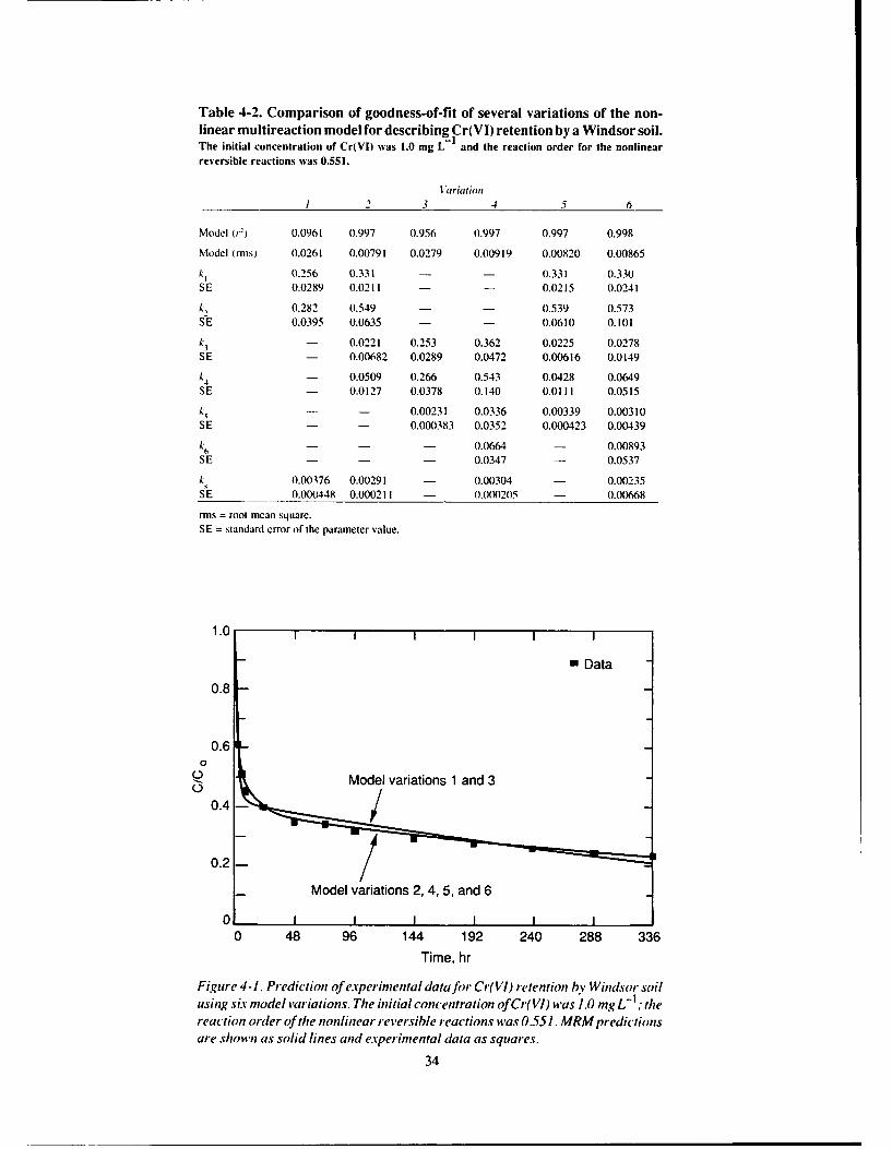
Table 4-2. Comparison of goodness-of-fit of several variations of the non-linear multireaction model for describing Cr(VI) retention by a Windsor soil.Trhe initial concentration of Cr(Vl) was 1.0 mg L_ and the reaction order for the nonlinearreversible reactions was 0-551.

Variationl

1 2 3 4 5 6

Model (r') 0.0961I 0.997 0.956 0.997 0.997 0.998

Model (rms) 0.0261 0.00791 0.0279 0.00919 0.00820 0.00865

k. 0.256 0.331 - - 0.331 0.330SE 0.0289 0.0211 - - 0.0215 0.0241

k,0.282 0.549 - - 0.539 0.573S E 0.0395 0.0635 - - 0.0610 0.101

k3- 0.0221I 0.253 0.362 0.0225 0.0278SE - 0.00682 0.0289 0.0472 0.00616 0.0149

k4- 0.0509 0.266 0.543 0.0428 0.0649SE - 0.0127 0.0378 0.140 0.0111 0.0515

k5- - 0.00231 0.0336 0.00339 0,00310SE - - 0.000383 0.0352 0.000423 0.00439

k,- - - 0.0664 - 0.00893SE - - - 0.0347 - 0.0537

k 0).00 376 0.00291 - 0.00304 - 0.00235SE 0.000448 0.000211 - 0.000205 - 0.0068

rms =root mean square.SE =standard error of the parameter value.

1.0 I

N Data

0.8

0.60

Model variations 1 and 30.

- Model variations 2, 4, 5, and 6

0 48 96 144 192 240 288 336Time, hr

Figure 4- 1. Prediction of experimental data for Cr(VI) retention by Windsor soilusing six model variations. The initial concentration of Cr( VI) was 1.0 mg L- thereaction order of tile nonlinear reversible reactions was 0.55 1. MRM predictionsare shtown as solid lines and experimental data as squares.

34

if independent experimental evidence warrants additional reactions. Generally. the model variation with theleast number of parameters that will adequately describe the data with low parameter standard errors is the mostdesirable.

Cr and Cd retention kineticsA three-parameter (one nonlinear reversible and one first-order irreversible reactions) and a five-parameter

(two nonlinear reversible and one first-order irreversible reactions) version of the MRM were used to predictexperimental data for the retention of Cr and Cd by several soils and at several initial solution concentrations.Selected results for several soils at one initial solution concentration and for one soil at several initial solutionconcentrations are listed in Tables 4-3 and 4-4 as examples for Cr and Cd, respectively. Other initial solutionconcentrations for the other soils gave similar results. The model was not used to fit the Cr retention data forthe Norwood orCalciorthid soils because very little Cr was retained by these high-pH soils and the experimentaldata were too variable. Best-fit three- or five-parameter model-predicted curves are shown in Figures 4-2 to4-5 along with the experimental data points. The five-parameter model was used in the figures only if the pre-diction was significantly better than the three-parameter version.

Either the three- or five-parameter model variations, depending on the initial concentration, predicted thedata adequately with low standard errors for the parameters in the majority of cases (Tables 4-3 and 4-4). For

10 1 1~Webster

1 Olivier-

-Jcz Molokai

E 0.1 Figure 4-2. Prediction of experim en-

Sharkey tal data for Cr(VI) retention by sevenLafitte soils. The initial Cr(VI) concentra-

0.01- tion for the Cecil, Olivier, Sharkey,Lafitte, and Molokai soils was 1.0 ing

L-I ;for the Kula and Webster soils it

0.0 was 10.0 mg L I. MRM predictions

0 48 96 144 192 240 288 336 are shown as solid lines and experi-Time, hr mental data as symbols.

Cecil

Norwood

E 0.117 ------A

-- ~ ~~Olivier -- a .. I

Sharkey

Figiure 4-3. Prediction of experimen-0.01 I I taldataforCdretention hyfour soils.

0 48 96 144 192 240 288 336 The initial Cdcolcentration was 1.02

Time, hr ing L-

35

Z.I -r 1 - -- Z. -t l

-- -7 -- 7

or L.

IC- Z2~ ~ C''

-m 2 £ 2 I = . e C

co C-- . D- -71-o - -rF-rr-

I - Cl Cl ' C

°14

a > r I

'S-- Cl - ,?C---l

"'"- -- - It> rI" -I . - ? "' . .. " -7 - Cl' e-l' -

O Cle.,l - F-- - ,

-- I . - _l l

36

E ..

.t-.. .;

- o. . .

r-I -- =.. . . -r _ .r. - - X +

F- . .. -F- - -t -- ,

. , -.- '. . -- _ -. -

f-I.7

I I I I I I

100 C/Co =100

7550

25

10

10

5 41 Figure 4-4. Prediction of eqwri-

2 mental data jO" Cr( r('tention

by Windsor soil. The initial Cr 7)

1 Coice'lntratiansfir the t(17 to the

0.1 bottom curves were 100.0. 75.0.0 48 96 144 192 240 288 336 50.0, 25.0. 10.0, 5.0. and 1.0 nix

Time, hr L- 1, respectively.

100 C/C 0 = 100

5010

10

9.02M 1.02

E

0.1 Figure 4-5. Prediction aJ experi-0.116 mental data for Cd retention bY

001 . Windsor soil. The initial Cd can-

0.01= 0.026 centrutionsfir the top to bottom

c(Uhf'S welt'e 100.0. 50.0, 10.0,

5.02, 1.02. 0.516. 0.116, 0.066,

0 48 96 144 192 240 288 336 04026. and 0016 mC . res/'e-Time, hr tivelv.

data sets where the model could not be fit to the data. a poor fit of the model to the data was obtained. Where

unacceptably high parameter standard errors were obtained, a number of reasons can be cited:" The model is an inaccurate representation of the reactions that occur.• The model underfit the data (too few parameters),

" The model overfit the data (too many parameters).

" The experimental data was too variable, and/or• There were too few data points.

Each of these points is discussed below with supporting examples.The model is an inaccurate representation of the reactions that occur; it does not describe accurately Cr

retention in the Kula and Webster soils at low concentrations, indicating the need fora different model forthesesoils. The MRM could not be fit to the data for Cr retention by the Kula and Webster soils at an initial solution

concentration of 1.0 mg L . Furthemlore, the parameter standard errors for the three- and five-parameter modelpredictions for Cr retention by the Webster soil at an initial concentration of 10.0 mg 1 are greatly inflated

(Table 4-3).The three-arameter mod'l undeijit the data. The three-parameter version of the MRM did not predict the

Cr retention data for the Olivier. Sharkey, and Molokai soils (C. = I mg L- I ) and the Windsor soil (C,, = 1.0.2.0. 5.0. and 10.0 mg L- 1) as well as the five-parameter model did, nor did it predict the Cd retention data for

the Windsor soil (C = 0.016. 0.026, 0.066. 0.116. 1.02. 5.02. 10.0. and 50.0 mg L - ) as well.

38

Tlwfiie-lpwrac'r mode'l aie~ffii th data. In most of these cases, lhe bet ter" fit of the five-parameter modelwas achieved without significantly increasing the uncertainty in tile parameter estinates, but in some cases tilebetter fit was achieved only with significant increases in the parameter standard errors. In many cases, however.where tile five-parameter version could not significantly improve the fit of the model to the data, the parameterstandard errors in the five-parameter version were inflated over those in the three-parameter version.

The e.NwrimentuIl data was too variable. In the case of Cr retention by the Windsor soil. the three-parameterversion worked best at higher solution concentrations and the five-parameter version worked best at the lowerconcentrations. At higher concentrations, only one nonlinear reversible reaction along with the first-order irre-versible reaction is needed to describe the data. This does not mean that an additional nonlinear reversible reac-tion is not occurring at the higher concentrations. If the extent of one of the reversible reactions is minor, thenit will not be observable at the higher concentrations.

Additionaldatapoints 'ouhlde nweded for these soils to produce rIel iable coefficients for the fastest reaction.The MRM could not be fit satisfactorily to the Cr retention data at initial concentrations of 150 and 200mg LI

because of data variability. In general. the model did not predict the experimental data at higherconcentrationsas well as at lower concentrations because of more variability in the experimental data. In addition, at higherconcentrations less time-dependent retention of Cr was observed. Moreover. the MRM did not work as well forCr retention by the Kula. Lafitte. Molokai. and Webster soils as it did for the other soils. Aside fiom the needfor a different model to describe Cr retention by the Kula or Webster soils, another reason for the poorer fit inthese cases is that fewer data points were available for model prediction. Nine data points were taken for thesesoils, while 12 points were taken for the other soils. The first data point for the Kula. Lafitte. Molokai. andWebster soils was taken at 24 hr. compared to 2 hr for the other soils. Thus. the standard errors of the rate coef-

ficients for the fastest nonlinear reversible reaction are large, since this reaction had reached equilibrium by tile

time the first data point was taken.The reaction order used for the nonlinear reversible reactions was obtained from the slope of regression lines

for log S vs log C after 336 hrof reaction time (Amacher et al. 1986). It was found that the slope of log S vs logC was less than I and did not change substantially with time after about 24 hr of reaction time. It was assumedthat the faster reversible react ions attained equilibriun within 24 hr. so that the react ion order for these reactionscould be calculated using the Freundlich approach (see eq 4- 1). It was also assumed that all the reversible reac-tions had the same reaction order (n = in). The model allows for the possibility that they are different (n # n).

At this time there does not appear to be a suitable experimental method by which the faster reversible reactionscan be separated and their reaction orders detenmined independently, nor is it known whether they are indeeddifferent or the same. This should be the subject of additional research.

The shapes of both the experimental data curves and the MRM predictions (Fig. 4-4 and 4-5) are influencedby tile initial metal concentration in solution and clearly illustrate that nonlinear (n and in * I ) and kinetic-typeretention reactions occurred. This behavior might also be attributed to possible changes in reaction mechanismsits the initial concentration changes. Furthermore, the magnitudes of the rate coefficients in Tables 4-3 and 4-4depend on the initial concentration. This indicates that although the model is successful in describing kineticdata fora given initial concentration. the same rate coefficientscannot be used todescribedata forsubstantiallydifferent initial concentrations. Thus, the model is an oversimplification and does not provide a complete de-scription of the actual processes that occur during retention-release of metals by soils. It describes only the time-

dependence of the concentration of metal in solution and the amounts retained by the various assumed reactionsites. In addition. only the loss of metal from solution was experimentally measured. Other components in tilereactions, such as the concentrations of the reaction sites and any ionic species exchanged by the retained metalions, were not measured. For a complete kinetic rate law, the time dependence of these components must bedescribed successfully. Thus. the model must be considered as a representation of an apparent rather than amechanistic rate law.

Release of Cr and CdThe MRM indicates that a fraction of the retained metal will be released to solution because the nonlinear

reactions are considered reversible. The model also indicates that another fraction of retained metal will not be

39

4.0

"7 3 .0

E: S2 , '2.0

2z Fiiure 4-0. MRM lpredictions oj"

tie tinme-depelident (ano)itI u]Crretained hv three phases (s s,

ands i) rfa ,indsm" soil. The ii-

tial Cr(1) concentration was 1.0

4 1i4 L22 3 ad the reUctiol ldCrfU"0 288 336 the nonlinear reversile rcactios

Time, hr was 0.55 /.

released to sol ution because of the irreversible retention reaction. The time-dependence of the amount ofCr (C

= 1.0mg L- ) retained by the individual soil phases (s. s, and )rr) for the Windsor soil is shown in Figure 4-6as an example. According to the model, some of the Cr originally retained by sI and s was released to solutionand subsequently retained by sirr . As expected. s reached maximum retention prior to the highly time-depen-dent s., while s. continued to increase with time.- rr,

Since the kinetic retention study showed that the overall retention of Cr and Cd did not reach complete equi-

librium after 336 hr of reaction, we can expect that the retention of these metals will not be fully reversible.Therefore, both the model and the retention data indicate that release of metal from the soil as a result ofdil utionof the soil solution cannot restore equilibrium ifthe reversible reactions have not yet attained equilibrium (Selimet al. 1976) or if there is an irreversible reaction.

1000 ' I I 1000 I

100-

01000

" • 0 10

E

0 0 0 0 *a

.6.50 0 * 0

10 * * * -

0) 5:: . . 0 a0,10

0.1 •

1 1 1 I I 1 t I z.._ 0 .0 1 n I I I0 96 192 288 0 96 192 288

Time, hrFiguse 4-7. Tiae-dependent reh'ase oj'CrundCdfrom u Windso" slutse veral intial'cn tra-

tions of r-etained metal.

40

This finding is supported by the experimental release data. Using the Freundlich model, Amacheret al. (1986)showed that when the soil solutions were diluted, the experimental data points did not define a singleretention-release isotherm, nor did they overlie the 336-hr retention data isotherm that would be required fora single reversible reaction at equilibrium. This hysteresis effect in sorption isotherms. which occurs during re-lease and upon dilution of the soil solution, was rigorously discussed by Selim et al. (1976) and has been ob-served by other investigators (Elrashidi and O'Connor 1982a.b; Peek and Volk 1985). The cumulative amountsof metals released as reported by Arnacheret al. (1986) indicated that substantial quantities of Crand Cd wereirreversibly retained by the soils and not released to solution even after 336 hrof release time. Furthermore, mostof the retained Cr could not be extracted with 0.01 M KH 2 PO4, which has been shown to readily replace ex-changeable Cr(VI) anions (James and Bartlett 1983). Most of the retained Cd could not be extracted with 0.5M Ca(NO 3 ). which indicates that much of the Cd was not exchangeable with Ca ions.

Additional insight into the reversibility of the retention of Cr and Cd can be gained by examining Figures4-7 and 4-8. In Figure 4-7. the amounts of Cr and Cd retained by the Windsor soil are plotted as a function oftime for several initial concentrations. The amounts of retained Cr and Cd at time zero for the release experiment

1.0L Cecil A Oliviero Sharkey E Windsor0 Kula 0 Webster0 Molokai

0.6 -

. .•o0 0' 0.4 -

*A AA

U 0~0.2 - A 0 {3A 0 0 o -

E0 0 0 A

1.0

A Cecil A Norwood0 Olivier U Sharkeyo Windsor

0.8

( 0.6 A 0

A. 0

t_0.4 0

a) Aa)~ 06

0 0 0 A

0.2 -

A A

lO 110 0 0

Cr Retained, mg kg' 1

Figure 4-8. Cumulative ainouts nf (tp) Cr- and (hottm Cid r-ehesedfr-om sever-al soils as a fiaction of the initial antoun ofilleta/ retail'd hythe soils at the start ofnietal r-ehase.

41

represent the amounts retained at the end (336 hr) of the retention experiment. Release of Cr and Cd occurredonly during the dilution phase of the release study (24-144 hr) (Figure 4-7). After 144 hr of release no furtherdilutions were done and the overall retention-release of metal appeared to have reached a steady state, sincelittle additional concentration changes were observed.

Release of metal occurred primarily when the samples with the greatest amounts of retained metal were di-luted (Figure 4-7). Little release occurred at the lower conce: trations. The extent of release is thus dependentupon the amount of retained metal. This can be readily seen in Figure 4-8 where the cumulative amounts of metalreleased over 336 hr are plotted as a function of the initial amount of metal retained by the soil at the start ofthe release experiment. In general, the cumulative amount of metal released increases as the amount of metalthat was originally retained increases. A possible interpretation is that at lower concentrations the metal ionsare retained by sites where they are more strongly held. whereas at higher concentrations they are retained bysites where they are more weakly held. There may be a range ui'metal-binding sites with different binding ener-gies. This can only be verified by independent experimental evidence, not by curve-fitting of a particular model.

Sensitivity analysisThe preceding examples show how the MRM can be used todescribe experimental kinetic data. At this point

it is worthwhile to consider how sensitive the results of the model are to the various model parameters. Figure4-9 shows the effect of incorporating different parameters into the model. The effect is primarily in the changeof the shape of the c vs time curves. The magnitude of such a change is determined entirely by the magnitudesof the model parameters. In some cases the effect may be large. while in others it is negligible. Recall that it waspossible to fit a number of model variations to the same experimental data set so that the results were virtuallyindistinguishable. Thus there appears to be a number of combinations of model parameters and variations thatoroduce nearly the same results, so a unique solution of our model for its prediction of a given data set shouldnot be expected.

The effect of changing the reaction order associated with s and s2 on model simulation curves is shown inFigure 4- 10. By decreasing the reaction order, the rate of the reaction is increased. For three curves shown inFigure 4-10 the reaction orders for both nonlinear reversible reactions are the same (n = i). while for others thereaction orders are different. The effect of the magnitude of the rate coefficients on the simulation curves for

1.0 I

1.k, = 0 1. k2 = 0.05. k=0.001 hr1

2. k, = 0.1. k2 = k3 = 0.05. k4 = 0.01. k, = 0.001 hr1

3. k3 = 0.1. k 4 = 0,05. k5 = O.C i hr1

0.8 4. k3 = 0.1. k 4 = k5 = 0.05. k6 = 0.01. k s = 0.001 hrI

5. k1 = 0.1, k2 = k3 = 0.05. k 4 = 0.01. k5 = 0.001 hr"6. ki =0.1, k 2 =k 3 =0.05, k 4 k 5 =0.01. k6 =0.005. ks=O.001 hr'

o 0.6U

0.4 Variations 2, 5, and 6Variations 1 and 3

Variation 4

0.2

00 48 96 144 192 240 288 336

Time, hr

Figure 4-9. Effect of model variations on model siulations. The parameters incorpo-rated into each model variation andl their mnagnitudes are shown in thefigure legenl.The reaction order for the nonlinear reversibhle reactions was 0.5.

42

1.0 I

0.8

n = m = 0.9

n 0.6=0.

0.4 m0.

0.2

0r0 48 96 144 192 240 288 336

Time. hr

Figu~re 4- 10. Effe ct oJ rection order onl model simulations. The reaction ordersUlsed ill thec Ilodl' simulautionls are sluon in tlu'figure le-endc, The Inainitucles of

1.0 I

0.8

o 0-6

0.4

0.20. 1.0.05.0.01.0.005, 0.001

0.1.1 0.05. 0.05, 0. 1. 0.001

0 10 48 96 144 192 240 288 336

Time. hr

Fi,iiure 4-Il1. Effecto(f rate coefficients on ,nodl'sinilatiouis. T/ie reaction orderfort the nonlinear reversible reactions it-is 0.5.

a given model variation is shown in Figure 4-l1. As the magnitudes of the rate coefficients decrease, so do thereaction rates. By adjusting the rate coefficients. an almost infinite array of curve shapes is possible. Note thatin Figures 4-9. 4- 10. and 4-1l. the curves are not appreciably affected by thle model parameters at short reac-tion times. Only at longer times do the curves become separated.

Mechanism consistent with modelAs previously discussed, it is not possible to deduce reaction processes that occur whien soils retain metal

ions based solely on model predictions of the loss of metal ions from solution data. Alternative processes may

43

give rise to the same experimental observations. This point was discussed by Skopp (1986) in his review of time-dependent processes in soils. Sposito (1986) pointed out that the complexity of the processes that occur whenions are retained by soils defies unambiguous interpretation by simple models. The physical and chemical pro-cesses that comprise reaction mechanisms occur at the molecular level, but experimental observations on soilsystems are nearly always at the macroscopic level. Furthermore, reaction mechanisms can never really beproved, only disproved if suitable experiments can be designed to rule out unambiguously a particularmechanism.

Despite these difficulties, mechanisms can be proposed that are consistent with the model and experimentalobservations. Harter (1984) proposed that the most rapid reversible retention reaction was nonspecific ionexchange, whereas the slower retention reaction was specific sorption of metal ions by soil surfaces. Thesereactions may also be interpreted in terms of formation of outer-sphere and inner-sphere complexes with soilsurfaces (Sposito 1984). This interpretation is entirely compatible with the MRM model. Harter's experimentaldata was taken at very short time intervals using a batch reactor (Zasoski and Burau 1978). The method usedin this paper is only suitable for highly time-dependent or slow reactions. However, the applicability of themodel is independent of the time-scale of the experiments, since there is probably a continuum of reactionscovering a wide time period. The model curve must still pass through the data points regardless of when theyare taken, although the fastest reactions may be complete before the first data point is taken.

Amacher et al. (1986) proposed that the irreversible or very slowly reversible retention of Cr, Cd, and Hgmay be precipitation or coprecipitation, internal diffusion, or, in the case of Cr and Hg, a change in the chemicalspecies (oxidation or reduction). Mendoza and Barrow (1987) proposed that the continuing reaction betweenphosphate and soils is the penetration of adsorbed phosphate into the adsorbing surface. This would be identicalto the internal diffusion process, which was also proposed by Aringhieri et al. (1985) to explain why a singlesecond-order reversible reaction could not adequately describe Cu and Cd retention kinetics. However, actualidentification of the chemical species and reaction sites is necessary to distinguish among the variouspossibilities, and such independent experimental evidence is for the most part lacking in the case of reactionsat soil surfaces. Greater progress has been made in studying reactions at pure mineral surfaces (Davis and Hayes1986). Nevertheless, the reaction mechanism proposed by Harter (1984) and extended to include otherprocesses by Amacheret al. (1986) is fully consistent with a vast body of soil chemistry literature, and the MRMis compatible with this interpretation.

44

Chapter 5. Retention Kinetics of Mercury in SoilsUsing the Multireaction Model

Numerous papers have examined various aspects of the geochemistry of mercury in water, sediment, and

soil (Hem 1970. Jenne 1970. Klein and Goldberg 1970. Thomas 197 1. Cranston and Buckley 1972. Frost andBisque 1972. Gay is and Ferguson 1972. Thomas 1972. Lindberg and Harriss 1974, Reimers and Krenkel 1974.Crecelius et al. 1975. Schindler and Alberts 1977. Anderson and Smith 1977. Eganhouse et al. 1978. Hogg etal. 1978. Gambrell et al. 1980, Harsh and Doner 1981). A few general conclusions can be drawn from thesestudies. Mercury (Hg) can be involved in a complex series of chemical and biological reactions in natural envi-ronments. Many of these reactions involve changes in the oxidation state of Hg. The chemistry of Hg in water.sediment, and soil is intimately linked to the organic matter in those phases. Organic matter appears to be the

single most important component in the environment that controls the chemistry of Hg. including retention andoxidation state transformations. Retention of Hg by soil and sediment occurs by sorption onto manganese oxides

(Lockwood and Chen 1973), iron oxides (Kinniburgh and Jackson 1978. lnoue and Munemori 1979). clay(Newton et al. 1976). and organic matter (Crecelius et al. 1975. Eganhouse et al. 1978) and by precipitation of

sulfides (Harsh and Doner 1981).

Methylation. reduction, and volatilization are the more important reactions involving changes in Hg specia-tion. Methylation of Hg(1I) occurs in anaerobic and aerobic environments and appears to be both a biological

and an abiological reaction (Langley 1973: Jacobs and Keeney 1974: Rogers 1976. 1977). Rogers (1977)showed that fulvic acid can methylate Hg(I). but humic acid cannot. Thus. abiotic methylation of Hg(I[) is a

potentially important reaction. Reduction and volatilization is microbially mediated and apparently does notoccur abiotically (Rogers 1979. Rogers and McFarlane 1979). Avotins and Jenne (1975) also report that Hgvolatilization involves microbes. However. Alberts et al. (1974) showed that humic acid could reduce and vola-

tilize Hg(ll).It is apparent from the foregoing discussion that the reactions of Ho in the soil environment are quite complex

and can involve several chemical species of Hg and retention by several solid phases in soils. Thus, multireac-tion models are needed to describe the chemistry of Hg in soils, especially where retention by multiple phasesis occurring. Recently. Amacher et al. (1988) showed that a nonlinear multireaction model could su-cessfully

describe the time-dependent retention of chromium (VI) and cadmium by soils. The success of this model indi-cates that it has potential applicability in describing Hg retention reactions in soils involving a single Hg species.In a previous paper Amacher et al. (1986) showed that single-reaction models failed to describe adequately thekinetics of HgCI retention by soils. In this chapter we test the ability of the multireaction model (MRM) to de-

scribe the time-dependent reactions of mercuric chloride by several soils at several initial concentrations. Acomplete description of the multireaction retention model (MRM) was presented in Chapter 3. In Chapter 4.

the MRM was evaluated for the prediction of Cr(VI) and Cd retention in several soils. In this chapter. we discussthe major differences in model predictions for Hg and those obtained previously for Cr(VI) and Cd.

EXPERIMENTAL AND DATA ANALYSIS

SoilsSoils used in this study are listed inTable 5-I along with their taxonomic classification and selected chemical

properties. The soils were air-dried and passed through a 2-mm sieve before use. The methods used to obtain

the chemical property data are given in Amacher et al. (1988).

45

Table 5-1. Taxonomic classification and selected chemicalproperties used in the Hg retention-release studies.

OrganicSoil matter CI-C Fe ,0

series Classfication, pit (c) (0'mol+ kg 1) (17c%)

Cecil Clayey. kaolinitic, thernic 5.1 0.24 3.7 10.2Typic Hapludulh

Norwood Fine-sily. mixed calc.), 7.4 0.32 6.2 0.44thermic.Typic Udilluvent

Olivier Fine-sily.mixedthermic 6.4 0.99 8.3 1.14.Aguic Fragiudalf

Sharkcy Very fine. nontmorillonitic, 5.4 1.69 31.3 0.94nonacidic, thermicVertic Haplaquept

Windsor Mixed, nesic. Typic 5.4 0.94 1.2 2.20Udipsamment

Reagents

Reagent-grade mercuric chloride, calcium chloride dihydrate, and potassium dichromate were used. Arainuld of Ho ( 23H .5x10 3 B -radionuclide of Hg (-_ Hg. 3.56 × I Bq kg - , HgCI, in 0.5 M HC) was used as a tracer to follow the extentof the Hg retention reactions.

Procedure

Retention and release of HgCl, was studied using the batch method outlined by Amacheret al. (1986). Initialsolution concentrations of Hg were 0.007,0.012,0.052,0.102,0.502, 1.00, 5.00, 10.0,50.0, and 100.0 mg L -

in 0.005 M CaCI,., The - '-Hg concentration in each solution was 7.4 x 105 Bq L- 1.

Calculations using species formation constants given by Lindsay (1979) revealed that, at the chloride andmercury concentrations used in this experiment, dissolved HgCI, was the predominant species. Thus, the reten-tion of essentially a single Hg species was being studied. To help maintain oxidizing conditions and to inhibitreduction and volatilization of the Hg(II), the solutions also contained 0.005% Cr(VI). The intent was to keepHg in a single form in solution throughout the course of the experiment.

The retention experiment was carried out as follows. Duplicate 4.0-g samples of each soil were added to pre-weighed 50-mL Teflon centrifuge tubes. Then 40 mL of each Hg solution was added to the duplicate samplesof each soil, and the samples were vortex-mixed. The centrifuge tubes were placed endwise in a box on a shakerset to shake at 120 osc min - .The samples were shaken for 15 min every 6 hr. After 2. 5, 8, 24,48, 72,96. 144,192, 240, and 288 hr. the samples were centrifuged for 10 min at 1300 x g. 25.0 mL of each supernatant waswithdrawn for radionuclide counting, the pH of the supernatant was measured, and the samples were reweighed,vortex-mixed, and returned to the shaker.

Release of retained Hg from the soils was initiated by diluting the solutions in contact with the soils. After336 hr of reaction between the soil samples and Hg solutions, the samples were centrifuged for 5 min at 1300

x g, 20.0 mL of each supernatant was withdrawn (of which 1.0 mL was used to count the 23 Hg), the pH of theremaining supernatant was measured, and 20 mL of Hg-free 0.005 M CaCI, were added to each sample. Thesamples were reweighed, vortex-mixed, and returned to the shaker. The centrifuging, 20.0-mL aliquot with-drawal, pH measurements, addition of 20.0 mL of Hg-free CaCI 2 solution, reweighing. vortex-mixing, andshaking steps were repeated four times at 24-hr intervals. The soil samples were again centrifuged, 0.5 mL ali-quots of each supernatant were withdrawn for radionuclide counting, the pH of the supernatant was measured.and the soil samples were reweighed, vortex-mixed, and returned to the shaker.

These steps were repeated four times at 48-hr intervals. Thus, both the retention and release of Hg were eachfollowed for 336 hr of reaction time. There were a total of five dilution steps at 24-hr intervals for the release

46

experiment, and release of Hg was followed for an additional time period after the dilutions were made.The activity of 203 Hg was counted by liquid scintillation spectrometry. Correction for radionuclide decay

was avoided by counting the aliquot of the original Hg solutions each time samples were counted. To correctfor losses of Hg due to sorption onto the Teflon tubes and volatilization from solution, 40 mLof each Hg solutionwas added to 50-mL Teflon centrifuge tubes without soil in them, and these soil-free samples were carriedthrough the entire experimental procedure. These corrections proved to be minor.

Data analysisDetails of the calculations of 'he ah,vuijs ot mercury retained and released by the soils are outlined in

Amacher et al. ( 986). Concentrations of mercury in the sample solutions were calculated from the specific ac-tivities of the initial solutions and the measured activities of the sample aliquot. The amounts of Hg retainedby the soils were calculated from the differences between initial concentrations in solution and the concentra-tions in solution at each sampling time, with a small correction for the amounts removed for counting. Theamounts of Hg released by the soils as a result of diluting the soil solutions were calculated from the solutionconcentrations at each sampling time during the dilution steps, with a correction for the amounts remaining inthe diluted solution. The amounts of Hg released by the soils after the dilution steps were calculated from thesolution concentrations at each sampling time, with a small correction for the amounts removed for counting.

The rate coefficients for the nonlinear multireaction model were obtained using a nonlinear, least-squares,parameter-optimization method (van Genuchten 198 1). This method is basically the maximum neighborhoodmethod of Marquardt (1963) and is based on an optimum interpolation between the Taylor series method andthe method of steepest descent (Daniel and Wood 1973). The criteria used for estimating goodness-of-fit of themodel to the data were the r-square and the root mean square statistics. The extra sum of squares principle(Kinniburgh 1986) was used to determine if there were any statistically significant improvement in the fit ofthe model to the data by adding more parameters to the model (e.g.. one vs two nonlinear reversible reactions).Additional details have been given in Chapter 4 and are also available in Amacher et al. (1988).

MODEL EVALUATION

The reaction order for the nonlinear reversible reactions was obtained from the slope of regression lines forlog total s (s1 + s + s.) vs log c after 336 hr of reaction (Amacher et al. 1986). An example is shown in Figure5-1 for the Cecil soil. Results from the other soils provided similar figures. The slope of log s vs log c at eachreaction time was <I (nonlinear) and did not change significantly with time after about 24 hr of reaction time.It was assumed that the reversible reactions attained equilibrium after 24 hr, so that an estimate of the reactionorder for these reactions could be obtained using the linear form of the Freundlich equation (log s = logK + nlog c). It was also assumed that the reaction orders for all reversible reactions had the same numerical value (n= mi). although the model allows for the possibility thatthey have different values. However, there does not ap- -

pearto be a suitable experimental method todetermine the Y 00.00actual number of reversible reactions and their reactionorders and rate coefficients separately and independently. - '

The results of the parameter optimization method for D .,obtaining the rate coefficients are listed in Table 5-2. The Zfit of the model to the data is illustrated in Figures 5-2 0 0'0

through 5-6 for the five soils. Two variations of the model 0010.001 0.010 0,100 1.000 0000 100.000

were used in describing the data: a three-parameter ver-sion(k,k 2,k)consistingofonlyonenonlinearreversible Hg Tn solution, rg

reaction (eq 3-2). an irreversible first-order reaction (eq 3- Figure 5-1. Mercuric chloride retention iso-4), and a five-parameter version (k I , k2, k 3. k4 , ks) consist- thernsfin" Cecil soil at each sampling tiniefioling of two nonlinear reversible reactions (eq 3-2 and 3-3) 2 to 336 hr.

47

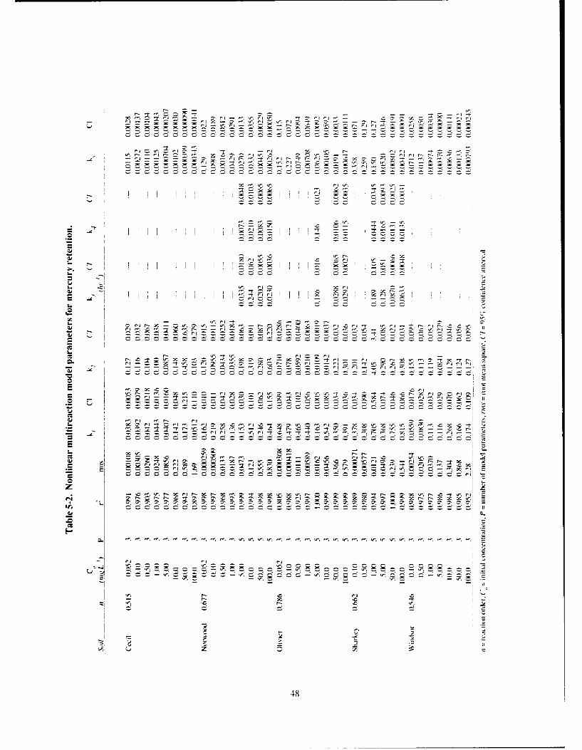
. . ..- -..... '-.-..... r r -

_- r r,-,-7.-z.- _. , - _r. -, _ _ _E - ~,e=,

'S'-- r r E

- - - E r . " -z = . . . . . . , .. ..

Er .. r-

-- ... I

. . . . . . . . ociI '-, __-__ciCu *.I -i- -- II

. .

~ c-i

1:= + + +

c-. r.-j Er.c-IC~48

1000, -o oall { o 0 0-.- - - , : 00.0_ .0 0 6oI0e----------*--- -- 0 0"0 -e-----3-j0 -

0 0

01 4:

- .OE-2 C

I. I-

I .0E-3 __ ---.- 4----- - _0 48 96 144 192 240 288 336 0 48 96 i44 i92 2 4: 288 336

Time, hr Tine, hr

Figure 5-2. Time-dependent HgCl, retention by Figure 5-3. Time-dependent HgClC retention b"

Cecil soil. The data points are shown as circles Norwood soil.and the model as a solid line.

0) 10.0

07

03

._ oo .o. . *,0.10. ,

~10E-0I OE-2

Z 'w l , .... .

"- .-- 2-.- r "4 °-- & : "M I tto3 I.E-

.CE.-4 1.CE-3 -'0 48 96 144 192 240 288 336 0 48 96 144 192 24C 288 336

Time, hr Time, hr

Figure 5-4. Time-dependent HgCI, retention by Figure 5-5. Time-dependent HgCI, retention byOli0ier soil. Shrkev soil.

E 1 o.0 ' -o _

S 1.0-

I) OE-3--I OE-4 -

0 48 96 144 192 240 288 336

Time, hr

Figure 5-6. Time-dependent HgCl, retention byWindsor soil.

and the irreversible first-order reaction (eq 3-4). The five-parameter version is reported in Table 5-2 only if itwas found to give a statistically better fit to the data than the three-parameter version according to the extra sumof squares principle. Otherwise the three-parameter version is shown.

It is apparent from the r-square and root mean square statistics in Table 5-2 and from the figures that the modeldescribes the data quite well for the initial concentrations shown. The 95% confidence intervals for the indi-vidual rate coefficients were for the most part reasonable, except in those cases where the experimental data didnot fit a smooth curve, so considerable uncertainty in the values of the rate coefficients was observed.

Some dependence of the rate coefficients on the initial Hg concentration was observed, especially when com-paring values at the highest and lowest initial concentrations. The shapes of the experimental data and modelcurves were also dependent on the initial Hg concentration. This indicates possible changes in the number andtype of retention reactions as the initial concentration changes. Since Hg is retained by a numberof solid phases

49

in soils, it is likely that a range of other types of reaction sites is encountered. At low Hg concentrations, notall the sites will be filled, but at higher concentrations, some types of sites may be completely filled while othersare only partially filled, depending on the affinity of the sites for Hg. This can account for the varying shapesof the time-dependent retention curves as the initial concentration increases. Because the model is probably asimplified representation of a complex series of reactions, the rate coefficients obtained by fitting the model tothe data should not be considered those for elementary reactions that comprise the reaction mechanism. Theyare probably apparent rate coefficients for a number of reactions of similar type.

For the Cecil and Windsor soils, which showed the least retention of Hg, the three-parameter model was ade-quate for all the initial concentrations listed. The five-parameter model provided improved description of thedata at the higher Hg concentrations for the Norwood, Olivier. and Sharkey soils. This behavior is quite theopposite of that observed for Cr(VI) and Cd retention by these same soils (Amacher et al. 1988). where the five-parameter version was found to work best at lower concentratio-ts. The additional reaction needed at higher Hgconcentrations may be due to the presence of other types of sorption sites not encountered (or inaccessible) atlower Hg concentrations or to the formation of an insoluble Hg phase. However. the fit of the model to the datacannot be used as proof of this since a numberof retention reactions may account for the co.itinuing loss of Hgfrom solution, including precipitation, internal diffusion, orsome species transformation reactions. It is not nec-essary to postulate a specific reaction in order to use the model to describe the data, however, since it is a general-purpose model that does not rely on a specific reaction mechanism. These points were discussed in detail byAmacher et al. (1988) and Selim and Amacher (1988).

The model did not fit the data at the lowest initial Hg concentrations (<0.052 mg L-I for the Cecil, Norwood,and Olivier soils and <0. 10 mg L-1 for the Sharkey and Windsor soils: data not shown). There was some evi-dence of the formation of a labile Hg species at the lowest concentrations of Hg. since after an initial decreasein Hg concentration upon reaction with the soils in tne retention experiment, a slow increase in He concentrationin solution was observed over time as Hg was releasedfrom the soils back into solution. The Hg release wasgreatest for the Cecil soil and was much less for the othersoils. The identity of this labile Hg species is unknown, 0)butinviewoftheknownbiologicalandabiologicalmeth- m 0 8ylation of Hg in soils, this is a likely possibility. Experi- E ,0.00T 0 0 0

_0 6 0 0 00 0mental methods for determining different Hg species Q P 0 0 0 0 C 6

would need to be used to determine the identity of the v , 8 8 8 8 8 8 S 8labileHgobservedattraceconcentrations.Theformation 0.,0o: 0 0 0 0 0 C C 0

of labile Hg occurred despite the presence of 0.005% po- O0.01 -

tassium dichromate, which was added to the solutions to 0 48 96 144 '92 240 288 336

inhibit reduction and volatilization of Hg. The concentra- Time, hrtion of this labile form of Hg was minor relative to thetotal Hg concentration in the solution, and its presence did fireo Cecil soil.not interfere with the application of the model to the dataat greater than trace concentrations of Hg. Inclusion of 60_o

species transformation reactions in the model would in- . o-oc, 0I-50.0 . /crease its usefulness at trace Hg concentrations, but rate No,,ood 7

coefficients for such reactions are lacking and need to be ) ,Wodso, C A

determined. 0 :"g 300 •

Incorporation of an irreversible reaction in the model 20.0 t/ /0(eq 4-4) is supported by the continuing loss of Hg from 00. / .

solution. Complete equilibrium was not attained in 336 hr C-- 0 0O

of reaction. The retention of Hg was not fully reversible, , 0.01 0.0 t .00 c 0 c ,QJ 00

as illustrated by Figure 5-7, which showsthe time-depen- Hg retaired, mg kg '

dent release of Hg from the Cecil soil. The other soils Figure 5-8. Cumulative nercury release as ashowed similar results. It is apparent that there was little function of retained mercury.

50

if any Hg release at the lower concentrations and that where release occurred, it was found primarily during tiledilution steps, since little release of Hg was observed after they were discontinued. Apparently, Hg release isextremely slow or does not occur at lower concentrations.

The cumulative amounts of Hg released expressed as a percentage of the amounts retained by the soils priorto the start of the release experiment were plotted as a function of the amounts retained. Figure 5-8 clearly showsthat Hg release is a function of the amount of Hg retained by the soil. Very little cumulative release of Hgoccurred at the lower retained Hg levels. This supports the existence of a range of different types of retentionsites with different affinities for Hg. At low amounts of retained Hg. virtually all the Hg is retained by high-affinity sites that will not readily release Hg when the soil solution is diluted. At higher levels of retained Hg.the high-affinity sites become filled and Hg is bound by lower-affinity sites that will release it when the soilsolution is diluted. The various soils also show different levels of affinity for Hg. The Cecil and Windsor soils.which retained less Hg than the other -oils. more readily released it to solution. The Norwood, Olivier, andSharkey soils showed about the same affinity for Hg. Only the cumulative release of Hg from the Norwood soilis shown in Figure 5-8. since the Olivierand Sharkey soils showed nearly equivalent results and overlapped tileNorwood results almost exactly.

The results of this investigation show that a nonlinear multireaction model is capable of describing the reten-tion of a single species of Hg by multiple soil phases. The model does not depend on any particular mechanismof solute retention, because the reactions in the model are distinguished solely on the basis of reaction rate: itis not necessary to have any prior knowledge of the retention processes to describe the data successfully. How-ever. tile fit of the model to the data does not prove any particular mechanism, since multiple processes can pro-duce the same experimental results. Independent experimental evidence is needed to identify the processesresponsible for element retention in soils. The model would have to be modified to include Hg species trans-formation reactions. including methylation and reduction-volatilization, to describe accurately Hg retention attrace concentrations. Independently measured rate coefficients for the Hg species transformation reactionswould greatly aid the use of the model, because attempting to fit too many rate coefficients at once results in

a poordescription of the data and yields poorly defined model parameters with excessively large standard errors.

51

Chapter 6. Predicting CR(VI) Transport Based on theMultireaction and Transport Model

For several heavy metals (e.g., Cu. Hg, Cr. Cd. and Zn). retention-release reactions in the soil solution havebeen observed to be strongly time-dependent. Recent studies on the kinetic behavior of several heavy metalsinclude Harter (1984), Aringhieri et al. (1985). and Amacher et al. (1986) among others. A numberof empiricalmodels have been proposed to describe kinetic retention-release reactions of solutes in the solution phase.

The earliest model is the first-order kinetic equation, which was first incorporated into the convection-dispersion transport equation by Lapidus and Amundson (1952). First-order kinetic reactions have been ex-tended to include the nonlinear kinetic type (van Genuchten et al. 1974. Mansell et al. 1977. Fiskell et al. 1979).A variety of other kinetic reactions are given by Murali and Aylmore (1983).

Amacher et al. (1986) found that the use of single-reaction kinetic models did not adequately describe thetime-dependent retention of Cr, Hg, and Cd for several initial concentrations and several soils. As a result,Amacher et al. (1988) developed a multireaction model that includes concurrent and concurrent-consecuti eprocesses of the nonlinear kinetic type. The model was capable of describing the retention behavior of Cd andCr(VI) over time for several soils. In addition, it predicted that a fracti.n of these heavy metals was irreversiblyretained by the soil.

The literature search revealed that no studies were carried out on the description of heavy ,netals transportin soils where the retention-release reactions are based on kinetic mechanisms. Amoozegar-Fard et al. (1984)may have been the first to investigate the mobility of Cd. Ni. and Zn using a fully reversible first-order kineticreaction. In this study, we modified the multireaction model of Amacher et al. (1988) and incorporated it intothe convection-dispersion transport equation. The model's ability to predict Cr(VI) mobility in several soilswas examined.

This chapter describes the transport behavior of Cr(VI) in six soils that have varying properties. We also testthe ability of the multireact ion and transport model (MRTM) for its ability to predict the retention characteristicsof Cr(VI) during transport. In addition, we investigate the use of kinetic retention parameters obtained frombatch experiments to predict Cr(VI) mobility in soils.

THE MODEL

A complete description of the multireaction approach for heavy metal transport and retention in soils(MRTM). including the appropriate initial and boundary conditions for the model and details of the numericalsolution used, is given in Chapter 3. A listing of the computer code for the model is given in Appendix B.

EXPERIMENTAL METHODS

Six soils were used to investigate the interactions and mobility of Cr(VI) in soil columns. The taxonomicclassification, mechanical size distribution, and selected properties of the soils are given in Table 6-1. The Bhorizon forthe Cecil soil and the Ap horizon of all other soils were used. The kinetic retention of Cr(VI) by thesesoils was investigated by Amacher et al. (1988) using the batch technique for a wide range of applied Cr(VI)concentrations. Selected results from this work are given in Chapter 4.

Miscible displacement experiments were used to study the mobility of Cr(VI) in the six soils. Each soil wasair-dried and passed through a 2-mm sieve before use. We followed the miscible displacement procedure de-scribed by Selim et al. (1987), where Plexiglas columns (4.4 cm in diameter x 6.35 cm long) were uniformlypacked with each soil to a given bulk density (Table 6-2). More than 20 pore volumes of 0.005 M Ca(NO')-were introduced into each column at a constant flux (Table 6-2) to equilibrate the soils with the background so-lution. A pulse of 100 mg L- 1 Cr(VI) in 0.005 M Ca(N0 3)2 solution was introduced into each column using

52

Table 6-1. Taxonomic classification and selected physical and chemical prop-erties used in the miscible displacement studies.

Olgullij8,,tl Sand Sill ('ho matt,,'! C-' I " )20

.N'rcS ('hixi/tatib l 1 p// ( j i f coa l+ 4, ) ('; l

Cecil C Ia\s,. kaol iniic. 30 19 51 5.1 o.24 3.7 10.2themic

Typic HapluduLh

Norotm ( Fi ne -siI,\. mixed 79 i8 3 7.4 10.32 6.2 0.44

(alc. ,thermicTypic Udil1uver

Olivier Finc-ihv. mixed. 5 89 6 6.4 (.99 8.3 1.14thennicAuuic Fraiudalf

Unnamed Calciorihid 70 19 I I 8.1 (.46 14.7 0.83

Webster Fine-loamy. mixed. 27 49 24 7.4 4.34 48.1 (.76nlmexlicT\ pic Haplaquoll

\Viiid,or Mixed, meic 77 20 3 5.4 0.94 1.2 2.2(

T% pic L'dipsaminn

Table 6-2. Soil parameters for the various soil columns ofthe miscible displacement experiments.

It ater BulkI'"ttent,'ll denlsit\'. Flhux.

Chlt,/un e p V Crf I puteitll niuihi'i' e c m ,, 4c m t /ftm 1) ilorevndttm e.)

Calciorthid 1(11 0.47 1.41 (1.14 2.611(0 (.48 1.37 1.08 2.3

Cecil 211 1.59 1.)8 0. 13 15.921(1 (.48 1.39 1.04 16.3

Normoixd 3101 0.42 1.72 0.14 2.53110 (.47 1.40 1.0.4 4.3

Olivicr 401 0.52 1.27 0.14 2.641(1 (1.53 1.25 l.0 3.9

Web,,er 511 0.62 0!.96 1.96 1.5

Windsor 60I (.38 1.65 (.17 4.9

611 (.42 1.53 1.13 3.7

a peristaltic tubing pump at a constant flux. A radionuclide tracer (3.7 x 109 Bq L-I S1Cr) was added to the Crsolutions to follow the extent of the mobility and retention reactions. The radio-labeled Cr(VI) pulse was fol-

lowed by several pore volumes of Cr-free background solution of 0.005 M Ca(NO3 )2 to elute the columns and

obtain a complete Cr(VI) breakthrough curve for each soil. A fraction collector was used to collect columneffluent. The 320 keV 51Cr peak was counted using gamma spectrometry. In addition, for each soil at least twoCr(VI) miscible displacement experiments or replications were conducted. Soil parameters associated witheach column experiment, such as v, p. 0. and volume of solute pulse (input). are given in Table 6-2. The dif-ference among replications for each soil is that significantly dff:rat fluxc:, i k ,,,ere a:.' '. js is commonly

carried out in miscible di:,pla,,ement studies.

To determine the hydrodynamic dispersion coefficient (D) for each soil. a pulse of tritium (C HO) andchloride-36 (- CI) was applied to each column prior to the Cr(VI) pulse. The volume of each pulse was equiv-alent to one pore volume. For both tracers, the background solution of 0.005 M Ca(NO 3 ), was maintained at

53

all times. Liquid scintillation spectrometry was 1.0 1 1 1 1 1 1 i ;used to count the chloride-36 and tritium radio- Cecl Ceci

tracers. 0.8 . (CL_-36) (tritium)

EVALUATION OF THE MRTM 0.6 /A prerequisite for the validation of a model is 0.4 \/

that the necessary model parameters be estimat- -

ed independently. In this study, we attempted to 0.2"

utilize. whenever possible, parameters that were " .

either independently measured or estimated by J o,

indirect means. Parameter estimates were util- ,.0ized for the kinetic rate coefficients from the Windsor Wndsor

0. -(CL-36) (triium)

batch studies of Amacher et al. (1988). Selectedrate coefficients are also given (see Chapter 4). 0.6-Other model parameters such as v, p, and E) wereexperimentally measured for individual soil 0.4'

columns.Values for the hydrodynamic dispersion co- 0.2 2

efficient (D) of eq 3-7 were obtained independ- -

ently from the tracer data for HO and6Cl for o0 C I 3

each soil. Selected results of YH20 and 36 CI v/v0Obreakthrough curves (BTCs) are shown in Fig-ure 6-1. These BTCs were interpreted using the Figuire6-1. Ch9loride-36atdtritiunrekthroughcurves

classical convection-dispersionequation(Selim (BTCs) for Cecil and Windsor soils. Solid curves are

and Mansell 1976): modelfittedBTCs.

R Dc/at = D 2 /. 2 - (4]6) c/av, (6-1)

where c = solute concentration (mg L - I)0 = soil water content (cm 3 cm- 3)

v = Darcy's flux (cm hr - )

D = hydrodynamic dispersion coefficient (cm 2 hr- I

x - soil depth (cm)

t = time (day - I )R = retardation factor,

R = I + p Kd/0, (6-2)

and Kd is the distribution coefficient (cm 3 kg- I ). Best-fit model parameters (Table 6-3) for D (and R) were ob-tained by use of the nonlinear least-squares optimization method of van Genuchten (1981). Estimates for Rvalues for the tracers were close to unity for all soils. R greater than unity indicates sorption or simply retarda-tion. whereas R < I may indicate ion exclusion or negative sorption. Similar values for R for tritium andchloride-36 were reported by Nkedi-Kizza et al. (1983), van Genuchten and Wierenga (1986). and Selim et al.(1987). Estimates for D were similar for the two tracers; therefore, a simple average value for D was used inthe transport model. Tracer results of Figure 6-1 also show little tailing of the BTCs. suggesting that the localequilibrium assumption for these soils, tracers, and water fluxes is valid (Rubin 1983).

Breakthrough curves forCr(VI) transport fron the mis.cible displacement experiments are shown in Figures6-2 to 6-9 for all soils. Results from Calciorthid, Norwood. and Webster soils show high peak concentrationsclose to unity (C/C 0 = I). with a sharp rise of the influent (or left) side of the BTCs. This was accompanied bylittle tailing of the desorption (or right) side of the BTCs. The times of arrival (or location) of the BTCs also sug-gest that little retention of Cr(VI) occurred in these soils. Moreover. the overall shape of these BTCs are similar

54

Table 6-3. Estimated dispersion coefficients (D) and retardationfactors (R) obtained from chloride-36 and tritium breakthroughcurves.

Chloride-36 (X 10- ) Tritium (x 10-4 )

Dispersion DispersionSoil coefficient Retardation coefficient Retardationseries (c1 2 hr -' ) factor ((c' 2 hr- ') factor

Cecil 0.172 ±0.0474 0.991 ±0.0496 0.173 ±0.0429 0.934 ±0.0409Norwood 0.074 ± 0.0334 0.955 ± 0.0066 0.085 ± 0.0384 0.997 ± 0.0714Olivier 0.054±0.0123 0.996:±0.0326 0.077±0.0074 1.021 ±0.0296Windsor 0.297 ± 0.0474 1.082 ± 0.0496 0.186 ± 0.0474 0.905 ± 0.0496Unnamed 0.054 ± 0.0095 0.942 ± 0.0169 0.066 ± 0.0161 1.034 ± 0.0312

to those for the nonreactive chloride-36 and tritiumBTCs of Figure 6- 1. For Olivier soil (Fig. 6-6), the I F T

BTC has a similar overall shape to the above three ° * a

soils with a high peak concentration and a moderate 0.8 - _tailing of the desorption side. However, there is a "shift to the right of the entire BTC, suggesting the °ooccurrence of retardation (sorption-desorption) dur- o

ing transport in Olivier soil. Such a retardation inthe arrival of Cr(VI) in the effluent was not ob- 04

served for the previous three soils.The BTC results of Figure 6-2 through 6-6 show

that for Calciorthid, Norwood, Webster, and Ol- G2

ivier soils approximately 100% of the applied Cr(VI)pulse was recovered in the effluent solutions. In . __Icontrast, for Cecil and Windsor soils (Fig. 6-7 2 / 0

through 6-9), the area under the BTCs indicate thatonly about 30 and 60% of the applied pulse was re- Figure 6-2. Measured (dots) and predicted BTCs forcovered, respectively. In addition, Cecil and Wind- Cr(VI) in Calciorthid soil (column no. 101).

sor BTCs show extensive tailing and a retardationof Cr(VI) in the effluent as well as a lowering ofconcentration maxima. These features strongly sug-gest kinetic (reversible and irreversible) solute re-tention (Selim et al. 1976. Rao et al. 1979, Nielsen

Norwoodet al. 1986). .0 - (e Experimental DotO

Reversible and irreversible reactions of Cr(VI) 0 p _in these soils may be the result of several retentionmechanisms, including physical adsorption. ion o.6-

exchange, formation of surface complexes, precip- U

itation, and coprecipitation (Bartlett and James 04 ,

1979. Amacherand Baker 1982, James and Bartlett o. v: o,4 ,m h-'

1983a,b,c). Irreversible retention, which is incor-porated in our model, is strongly supported by the o - 4 6 8

continuing reaction between Cr(VI) and the soils v/Voeven after 336 hr in the batch studies, the fact that Figure 6-3. Measured (dots) and predicted BTCsoverall retention was only partly reversible, andthe for Cr(VI) in Norwood soil at v = 0. 14 cm hr- Ifact that little retained Cr(VI) could be replaced by (colion no. 301). Curve A is the model predictionphosphate ions (Amacher et al. 1986). We postu- fora nonreactive solute and curve B isafittedBTClate that the irreversible reaction is caused by a re- using equilibrium (Freundlich) soiption (K,=

duction of Cr(VI) to Cr(ll). with possible precipi- 0.0475 cm3 g-1 and b = 0.952).

55

06 Fil,re 6-4. Measured (dots) am/ /)I(/ictd

BTCs. lr Cr( I\ ) in Nortvo soatil v = 1.04 cmhr (colunn no. 3 10). Dashed curve is model

0 2 V 4 c[ h, 4 - )ihredictiolfor a lun'ea clive solut' and .olie!L L curve is a fitted BTC using equilibrin (Fre-

00 2 4 6 a tindlich) .volPtioni (K/ = 0.0475 (m ,,- and bV/VO =0.952).

Webster

10

0.8

06 A

0.4 Figtire 6-5. Measured ((lots) amd neWdittetlBTCs fin Cr(l 7) in Webster soil (C'141ut1 no.

510). Curve A is niodel Ir(ediction using batchRuI' Coeff'i'ietsfinr C = /0 ig L- and clv

0I2 - B (dashed) is model 'esItsftsn" a n1onreactive0 1 .volute.

v/v

i I I [I 1

Olivier10- A-

8 N

0.8 , c .

\* E xper imentalo6 . Data

1l-- 0 (fitted) Fiiture 6-6. Measured (lots) and predi'cted

0.4 BTCs fin Cr(1) in Olivier soil (colint uIo.I \ 401 ). CurIve'sA , B. andCar'e mode/p~r'dictions

02 I using, batc/h rate coejficientsfior C( = /00. /0.02/ I -I.CUnd I nI,, L- , reswctivev. Curve D is a fitted

00 _ *>• "BTC tsin. Iranmeters obtained fioI least-

0V/V02 4 6 8 silmire' '.m ltim it lon.

WVo

ration of Cr(lll) on mineral surfaces or as discrete particles of hydrous Cr(ll) oxides. Organic matter. Fe(ll)minerals, and other possible reducing agents are known to irreversibly reduce Cr(VI) to Cr(Ill). Reduction ofCr(VI)toCr( I I) by organic matter is a slow process at nornal environmental pH and temperature levels as usedin this study. Moreover. theoverall reaction rate is pH-dependent (Amacherand Baker 1982). and the proposedirreversible term in the model (eq 3-13) is consistent with these observations.

The solid and dashed curves shown in Figures 6-2 to 6-9 are model calculations ofCr(Vl) BTCs for the mis-

cible displacement experiments. In the following discussion, predicted BTCs imply the use of independentlymeasured model parameters derived from the batch reaction studies (k I ./k " ' k K4 " and kI ) of Arnacher et al.(1988) that are given in Chapter 4. The predicted BTC shown in Figure 6-2 for Calciorthid was obtained withall rate coefficients set to zero. These values were selected since little or no sorption of Cr(VI) was previouslymeasured for all applied initial concentrations in the batch experiments. Therefore. the miscible diplacement

56

data are consistent with the data obtained earlier from the hatch studies. Moreover. model predictionls agreedlwell with thle experimental BTC: consequently. Cr( VI) transport may be considered similar to that ot a non1-reactive solute. In fact. the sorption side ofthe experimental BTC indicates early arriVal,whhsugt adreofniegiative reta rdat ionl (or ion exclIus ion) in theCalciorthid soil. Otherpossible reasons forearlv arrival ofBTC.mlay be tile presence of preferential (micro- vs macropore) flow and/or mobile-immobile reizions (van Gei-uchten and Wierenga 1976).

The use of a nonlreactive transport model also provided good predictions of the experimental BTC for Nor-wvood soil (Fi. 6-3). According to Amiacheret al. (1988). Ci-(VI) retention in Norwood was similarto Calcior-thid where little sorption was detected for these high pH soils. Improved BTC prediction was obtained whenthle nonlinear least-squares (best-fit) optimization scheme) (van Genuchten 198 1) Was used inl conjunction with

ourmdel As m-eult rhfitted BTC (solid curve in Fig!. 6-3) was obtained. which sugg~ests small CrI)rtntion inl this soil1. Actual best-fit parameter estimates were for K(, was 0.0475 + 0.0236 cmn' C and for b 0.952±0.092. The use of linear retention (i.e.. I? = I ) prov ided similar BTC predictions.

To illustrate the reliability of our- experimental results as well as the ver satility of our- model. C-( VI) resultsfor Norwood soil obtained under high flux (v* = I1.04 cm hr- . column no. 3 10. Table 6-2) wvere also examined.This is shown in Fiaure 6-4. where the use of a nonreactive transport model provided good agreement with theexperimental results. This findingz is consistent with that obtained previously for BTC results, from low flux (v= 0. 14 cm hK l) for the same soil shownl inl Fisrure 6-3. NMoreover. the use of fitted model parameters (K,, andh from the low-flux BTC provided equally good prediction for the high-flux BTC. as indicated by the solidcurve of Fioure 6-4. We should also point out that analyses of BTC results forother soil columns at high fluxes(not shown) were consistent with those for Norwood soil: refer to other studies on the intluenceof flux onl soluteretention during transport inl soils (e.g.. Selim et al. 1976. vanl Genuchten and Wieren-a 1986). Therefore, welimlit thle followine' discussionl to Cr-(Vf) transport inl columns under low fluxes (see Table 6-2).

Thle description of Cr transport for Webster soil (Fig. 6-5) was attempted in two different ways. Because ofthe overall -shape and location of thle BTC. we utilized a nlonreactive model to describe thle experimental data

A Cecil

k- k4 - c

Fi-m',,c 0-7. Mcuxiwe/ (dais) au,/ plIicwicd BTC.% filarpe-naC1.61I) ill cciil kod il (c/n0n. 201) uising, t/ie thi/c--)cl/l)cic' nad'/ (i.e.. k . = ki = 0). Curves A. B. C. D. aid

Cecil

FiI~un' 0-8 -Aleasuiccj (dots) alid /rcedicted BTC. ar - _____

C1.01I) ill Cecil Vail (ca/n'nn iuno. 210/) Ilsill"4 i/hc five-paraimier nUN/l. Curvces A. B. C. D. mid E are( moidelf' Ce

pr-editans ism. b 1.t cmfceisfn C /0 25 lited)

5. 2 im/l / im', dTnecivv/v. CuvF is ujitied BTC ]-1i51/H4 pual neiels obailllfi/l jeo- /ae piniz-ltin/i (ee Tlih/c 0-4). 85

57

(dashed curve). We also obtained model predic-r! A Widso tions using estimated parameters from the batch

, results and tile three-paraneter version of the

', /multireaction model (MRM). Specifically.

parameters k k. ii. and k, given in Table 4-3(Table 5 of Amacher et al. 1988) were used inU > I"EXperimenjol

the MRTM. Similarities of model predictionso.', \(solid curve) to the nonreactive BTC (curve A)

0.4'S"were not surprising. This is primarily due to the, , .. D (filed -

1 large k and k, values (0.948 and 1.08 hr-I': i~l ,/;" , t " " ";;-.',-. _ ... which suggest rapid retentiion-rlese react ions

oL - ." . , ":_--a ..------_ _ : j and thus closely resemble conditions for local

S4 83 12 16 equilibrium. In addition, the extent ofCr reten-V/ V tion was small due to the small values for the

Fi,ure 0-9. Measur-ed (lots) and predicted BTCs Jot order of reaction h (= 0.303) and , (= 0.00258C#'I) ill Windsor soil (columnt )1). Ctur-ves A, B, and C hr- ). Tile model estimated that only 0. V/( ofare model 1 #edicti~,s 11sittg' batch rate (0(iients fo) C, applied Cr was irreversibly retained by the soil= 2. 5, and 100 mng L- , respective/y. Curve D is afitted column after 4 pore volumes. The parametersBTC ising i'paan'eter-s obtainedJ)'om least-squares opti- used for model calculations were the batchmnization (see Table -3). results for an initial concentration (C) of 10 mg

0

L- .whereas a C of 1() mg L-1 was used in theapplied pulse to the miscible displacement columns. Model calculations using other coefficients for differentC were not performed because poor parameter estimates (highly inflated standard errors) were obtained using0

parameter optir lization. The use of the multireaction model to describe Cr retention in batch experiments was,therefore, not recommended for this soil. It is conceivable that poor parameterestimates are the result of the ex-tremely low Cr retention or lack of kinetic reactions as indicated by the shape of the BTC in Figure 6-5.

The predicted BTCs shown in Figures 6-6 to 6-9 for Olivier, Cecil, and Windsor soils were obtained usingdifferent sets of parameter values for the rate coefficients (k I, k 3 k 4. and ks) in tile transport model. This isbecause a unique set of values for the rate coefficients was not obtained from the batch data: rather, a strongdependence of rate coefficients on input concentration (Co ) was observed ( Amacher et al. 1988). For these soils,several features of the predicted BTCs are in common and suggest strong dependence on the set of rate coef-ficients used in model predictions. Increased sorption and decreased peak concentrations were predicted whenbatch rate coefficients from low initial concentrations (C ) were used. The dependence of predicted BTCs onrate coefficients from different C s is manifested for Cecil soil, whereas minimum influence was obtained for0Windsor soil.

From Figures 6-6 through 6-9. the use of batch rate coefficients at C = 100 mg LV , which is the concen-0

tration of Cr(VI) in the input pulse. grossly underestimated Cr(VI) retention by the predicted BTCs for thesesoils. In fact, for Olivier and Windsor soils, underestimation of Cr retention and thus overestimation of poten-

tial mobility of Cr in these soils was consistently observed for all sets of rate coefficients used. However, ferCecil soil, the use of sets of rate coefficients from low C s resulted in lower overall concentration in the effluentand predicted an increased retention in the soil column. This is a direct result of higher irreversible rate coef-ficients for Cecil in comparison with Olivier or Windsor soils. In addition, as C decreased from 1(0 to I mg

0

L- .ks values increased by more than two orders of magnitude (from 0.0(X093 to 0.211 hr '), which resulted inhigher amounts of Cr irreversibly retained by the Cecil soil as predicted with our transport model.

The model predictions shown in Figures 6-6 through 6-9 clearly illustrate the failure of the proposed modelto describe the transport data when independently measured model parameters were used. The reasons forthisfailure, which has been observed by other scientists, are not fully understood. A likely explanation is that theproposed model does not completely account for all reaction mechanisms or the reaction components presentin the soil system. Specifically. the model may be an apparent rather than a complete mechanistic rate law. Itis conceivable that tile strong dependence of rate coefficients on C ,as obtained from batch experiments. may

58

Table 6-4. Best-fit model parameters for miscible displace- also be due to additional mechanisms stillment experiments for Olivier, Cecil, and Windsor soils, ignored in the model. Invariant rate coef-

ficients with solution concentrations areP~granieter Olivie'r (ecil It 'i,;dur expected ifa complete mechanistic rate lawKd (n 1.616 ± 0.1439 2.614 ± 0.1747 15.292 ± 1.1123 is postulated. Amacher et al. ( 1988) consid-h 0.799 ± 0.0224 0.513 ± 0.0197 0,418 ± 0.0187 ered the rate coefficients to be pseudo rateki (hr 1) - 74.061 ± 1.3769 2.313 ± 1.1109 coefficients.

k, (hr -I 0.498 ± 0.0421 0.388 ± 0.2182 The dependence of BTC predictions on thea - 0.436 ± 0.2729 0.486 ± 0.1495 version of the model used to obtain thek, (hr 1 - 1.334 ± 0.1162 - necessary rate coefficients was also exam-k(r h - 0.016 ± 0.0019 - ned. as depicted by the predictions shownM - 0.455 ± 0.0172 in Figures 6-7 and 6-8 for Cecil soil. In4 (hr - 0.0156 ± 0.00551 0.0145 ±1 0.00979 Figure 6-7. the predictions were obtained

0.973 0.931 0.955 using the three-parameter model version

(i.e.. k3 = k4 = 0), whereas the BTCs inFigure 6-8 were obtained using the five-parameter version (see Amacheret al. 1988). It is evident that the use

of these two different model versions resulted in different model predictions, as clearly illustrated by BTCs Cand D in Figures 6-7 and 6-8. This is not always the case, however, based on predictions of retention data fromthe batch experiments as illustrated by Amacher et al. (1988). In fact, it was concluded that a number of modelvariations can produce similar model predictions of the kinetic batch results. In addition. Skopp (1986), Nielsenet al. (1986). and Selim and Amacher (1988) stated that use of alternative models to describe time-dependent

reactions may give similar predictions.

An excellent fit of a data set does not in itself constitute a proof of any specific retention-release reaction.Therefore. no efforts were made in this study to examine the capabilities of different model variations basedon curve-fitting alone. Instead, we utilized our transport model along with the optimization (curve-fitting)scheme to test its ability to describe the BTC from these soils without relying oil parameter estimates from the

batch experiments. Our hypothesis here was that a model gives an inaccurate representation of the reactionmechanism and should thus be discarded if it is completely incapable of describing experimental BTCs suchas those in Figures 6-6 through 6-9. The estimated parameter values that provided best fit of these BTCs aregiven in Table 6-4. For all three soils, the goodness of fit as measured by r- exceeded 0.90 (see Table 6-4).

Despite the fact that the model was incapable of predicting the BTCs shown in Figures 6-6 through 6-9 exceptby the use of curve-fitting procedures. some limited interpretations of the model description of the data and

associated parameters should be given. For Olivier soil the use of a nonlinear (Freundlich) equilibrium ratherthan kinetic retention reactions provided excellent BTC prediction with no apparent need for irreversible (sink-

term) sorption from the soil solution. Less than 0.1 'Ic of applied Cr was irreversibly sorbed when batch k. valuesirr

were used in BTC predictions (e.g.. curves A, B. and C of Figure 6-6) and thus is in agreement with modelcalculations based on curve-fitting only. For Cecil and Olivier soils, it was necessary to incorporate theFreundlich equilibrium sorption in addition to kinetic-type reactions to obtain the best-fit BTCs shown. Thisis manifested by the large K estimates obtained for these two soils. Equilibrium-type sorption-desorption

dreactions were not incorporated in the multireaction model of Amacher et al. (1988). Most striking, based on

parameter estimates given in Table 6-4. is that the order of reactions (b. n. and i) obtained based on best-fitpredictions were essentially similar foreach soil. Moreover, these estimated values were somewhat similar tothe order of reactions obtained from batch experiments. This is particularly true for Cecil soil and to a lesserextent for Windsor and Olivier. This finding implies that one order of reaction may be capable of describingall reversible retention-release reactions and that it may be determined from data analysis of batch experiments.

In addition, mechanistic models, which require fewer parameters. are extremely desirable since fewermeasurements need to be performed to determine such parameters independently.

59

Chapter 7. A Second-Order Two-Site Retention and Transport Model

In this chapter we present an analysis of a kinetic second-order approach for the description of heavy metalsretention mechanisms in the soil environment. This second-order approach will be incorporated into the non-equilibrium two-site model to simulate the potential retention during transport of heavy metals in soils. In Chap-ter 8 this approach will be extended to the diffusion-controlled nlobile-immobile (or two-region) transportmodel.

A main feature of the second-order two-site (SOTS) model proposed here is the assumption that there aretwo types of retention sites on soil matrix surfaces and that the primary difference between them is based onthe rate of the proposed kinetic retention reactions. We also assume that the retention mechanisms are site-specific. e.g.. the sorbed phase on type I sites may be characteristically different (in energy of reaction or theidentity of the solute-site complex) from that on type 2 sites. An additional assumption is that the rate of soluteretention reaction is a function not only of the solute concentration present in the solution phase but of theamount of available retention sites on matrix surfaces as well.

MODEL FORMULATION

Second-order kineticsFor simplicity, we denote sT to represent the total retention capacity or the total amount of sites on matrix

surfaces. It is assumed that sT is invariant with time. Therefore, based on the two-site approach, the total sitesconsist of two types such that

ST = ST + T2 (7-1)

where sTI and sT2 are the total amount of type I sites and type 2 sites, respectively. IfF represents the fractionof type I sites to the total amount of sites, we thus have

sI = FsT and ST2 = (I - F) ST. (7-2)

We now denote as the amount of unfilled or vacant sites in the soil such that

V1 = sT1 -S = F sT - s (7-3)

I2 = ST2 -S2 = ( 1 - F)sT - s, (7-4)

where 0, and 0, are amounts of vacant sites and s, and s., are the amounts of solute retained (or the filled sites)on type I and type 2 sites, respectively. As the sites become filled oroccupied by the retained solute, the numberof vacant sites approaches zero, i.e. (0, + 0.,) - > 0. In the meantime, the amount of solute retained by the soilmatrix approaches that of the total capacity (or maximum amount)of sites, (s, + s') ---> ST .

We commonly express the amount of solute retained, such as s, and s 2 ofeq 7-3 and 7-4. as the mass of soluteper unit mass of soil (M/M soil). Therefore, based on the above formulations. the amount of total sites VT. STI'and sT2 and vacant or unfilled sites 0, and ¢. must also have similar dimensions. Here the units used for s andf will be in terms of milligrams of solute per kilogram soil mass (ing kg ).

We propose that the retention mechanisms follow a second-order kinletic-type reactionwhere the forward process is controlled by the product of the solution concentration c (mg L- ) and the amount

60

of unoccupied or unfilled sites (0) (Selirn and Amacher 1988). Specifically, the reactions for type I and type

2 sites may be expressed by the reversible processes:

kic+ 411 <--> S 1 (7-5)

k,

and

k.c + ¢ , <- S . (7-6 )k 4

Therefore, the differential form of the kinetic equations of the rate of solute retention may be expressed as

Pas t= k, 1 c c-p k 2 s, for type I sites (7-7)

and

P a.lt = k 3 2 c- p k 4 s 2 for type 2 sites (7-8)

wherek andk, (hr-I) are the forward and backward rates of reaction for type I sites, and k and k are the co-I - ~3 3 4,3refficients for type 2 reaction sites, respectively. In addition, E is the soil water content (cm cm ) and p is

the soil bulk density (g cm-3). Ifo, and , are omitted from eq 7-8 and 7-9, the above equations yield two first-order kinetic retention reactions (Lapidus and Amundson 1952). However, a major disadvantage of first-orderkinetic reactions is that, as the concentration in solution increases, a maximum solute sorption is not attained,which implies that the soil has an infinite sofute-retention capacity orthat there is an infinite numberofexchange

sites on matrix surfaces. In contrast, the approach proposed here achieves maximum sorption when all unfilledsites become occupied (i.e., 0, and - -- 0).

In a fashion similar to the nonequilibrium two-site concept proposed by Selim et al. (1976), type I sites may

be regarded as those where equilibrium is rapidly reached (i.e., in a few minutes or hours). In contrast, type 2sites are highly kinetic and may require several days or months for apparent local equilibrium to be achieved.For type I sites, therefore. rate coefficients k I and k2 are expected to be several orders of magnitude larger thank3 and k4 of the type 2 sites. As t --- -,. i.e., when both sites achieve local equilibrium, eq 7-7 and 7-8 yield the

following expressions. For type I sites,

e k 1 c-p kS =0 as t--+, (7-9a)

or

s IO 10 = (EkIlpk,) = (o, as t -- cc (7-9b)

and for type 2 sites

Ek 3 p2 c-pk 4s 2 =0 as t -40 (7-1Oa)

or

.s/A0 c) = (E k3 4pk = ( ,1) as 1- -o , (7-1Ob)

Here 0)I and 0i2 represent equilibrium constants for the retention reactions associated with type I and type 2

61

sites, respectively. The formulations of eq 7-9 and 7-10 are analogous to expressions for homovalent ion-ex-change equilibrium reactions. In this sense, equilibrium constants o0 and o3, resemble the selectivity coef-ficients for exchange reactions and sT resembles the exchange capacity (CEC) of soil matrix surfaces (Sposito1981). However, a major difference between ion exchange and the proposed second-order approach is that noconsideration for other competing ions in solution or matrix surfaces are incorporated in the rate of reactions.In a strict thermodynamic sense, the above equations should be expressed in terms of activities rather than con-centrations. However, an implicit assumption is that solution-phase ion activity coefficients are constant in aconstant ionic strength medium. Moreover, the solid phase ion activity coefficients are assumed to be incor-porated in the selectivity coefficients (o and 0,) as in ion-exchange formulations (Sposito 1981).

We now consider the case where only one type of active site is dominant in the soil system. In a fashion similar

to the formulations ofeq 7-9 and 7-10, the kinetics of the reaction can be generalized by the following reversibleLangmuir equation:

p Ds/at = E k1.0 c - p kb. (7-Il)

Here k fand kb (hr - 1 ) are the forward and backward retention rate coefficients and s is the total amount of soluteretained by the soil matrix surfaces. Reaction 7-Il at equilibrium obeys the widely recognized Langmuir iso-therm equation

s/S T = KcI( I +Kc). (7-12)

where K = (19 kf/pkb) and K is equivalent to 0o of eq 7-9 and 7- 10. For recent discussions on the formulation ofthe kinetic Langmuir equation see Rubin (1983) and Jennings and Kirkner (1984).

It should be recognized that the unfilled or vacant sites (0) in eq 7-9, 7-10, and 7-11 are not really vacant.They are occupied by hydrogen. hydroxyl, or other nonspecifically (e.g., Na. Ca, chloride, nitrate) or specif-ically (e.g., sulfate, phosphate, transition metals) adsorbed species. The terms vacant or unfilhd mean vacantor unfilled by the specific solute species of interest. The process of occupying a vacant site by a given solutespecies actually is one of replacement or exchange of one species for another. However, the simplifying assump-tion on which this model is based is that the filling of sites by a particular solute species need not consider thecorresponding replacement of species already occupying the sites. The Langmuir-type approach consideredhere (eq 7-8 through 7-1I) is a specialized case of an ion exchange formulation. This was considered in detailby Elprince and Sposito (198 I). Alternatively, the competitive Langmuir approach may be used if the identitiesof the replaced solute species are known (Jennings and Kirkner 1984, Jennings 1987).

Transport modelIncorporating the second-order two-site reactions into the classical (convection-dispersion) transport equa-

tion yields (Selim and Amacher 1988)

p as Il/at + p Ds,/at + E ac'/t = E D 2.- v '/x - Q. (7-13)

Here the term Q is a sink representing the rate of irreversible heavy metal reactions by direct removal from thesoil solution (mg day- 1 cm-3 ). In this model, the sink term was expressed in terms of a first-order irreversiblereaction for reductive sorption or precipitation or internal diffusion as outlined by Amacher et al. ( 1986, 1988):

Q = 9 kc. (7-14)

where k is the rate constant for irreversible reaction (hri ). Eq 7-14 is similar to that for diffusion-controlledprecipitation reaction if one assumes that the equilibrium concentration for precipitation is negligible and thatk is related to the diffusion coefficient (Stumm and Morgan 1981).

For convenience, we define the dimensionless variables

X =x/L, (7-15)

62

T= vt/LE. (7-16)

C = c/Co (7-17)

S = S/ST. (7-18)

D= 0/ST, (7-19)

P = vL/D R, (7-20)

where Tis dimensionlesv tim ju:., alent to the numberof pore volumes leached through a soil column of lengthL, and P is the Peclet number (Brenner 1962). Given the above variables, eq 7-13, 7-7, and 7-8 are rewrittenin dimensionless form, respectively, as (Selim and Amacher 1988)

K2 [aS I/JT + aJS2/IT] + JC/T = (I/P) a2C/aX2 - aC/X - k sC (7-21)

aS/DT = ic IDI C - SI $1 (7-22)

S2/aT = K3 (D2 C - K 4 S2 (7-23)

where

2= sTP/CoE, (7-24)

K = k EL/v, (7-25)s s

K =k I &C 0L/pv and K3 = k3 e 2C0L/pv (7-26)

K 2 = k2L/v and K4 = k4eL/v. (7-27)

Here, K s, KI IK K 3' and K4 are dimensionless kinetic rate coefficients that incorporate v and L. As will be shownunder Transport below, these dimensionless variables (including K2, C, S, and (D) represent a convenient wayto study the sensitivity of the model to reduced variables.

For simulation and model evaluation, the appropriate initial and boundary conditions associated with eq 7-21 through 7-23 were as follows. We chose uniform initial solute concentration C. in a finite soil column oflength L such that,

C = C. (T= 0, 0 < X< 1). (7-28)

We also assume that an input solute solution pulse with a (dimensionless) concentration C was applied atthe soil surface for a (dimensionless) time T and was then followed by a solute-free solution. As a result, atpthe soil surface the following third type boundary conditions were used (Selim and Mansell 1976, Parker andvan Genuchten 1984):

1 =C-(I/P) C/lX, (X= 0, T< T) (7-29)

0=C-(0/P) C/aX, (X=0, T>T) (7-30)

and at x = L, we have

C/aX = 0 (X = 1, T > 0). (7-31)

The differential equations of the SOTS model are of the nonlineartype, and analytical solutions are not avail-able. Therefore, eq 7-21 through 7-23 were solved numerically using finite difference approximations (explicit-

63

implicit) subject to the above initial and boundary conditions. The numerical solution was compared to resultsobtained using a closed-form solution for linear type problems. For all cases considered, a mass balance wasmaintained as a check on the numerical results. Differences between calculated mass and the input for a solutepulse input were not allowed to exceed 3%. The resulting numerical scheme is documented in the SOTS modelprogram, which is written in Fortran.

Briefly, the convection-dispersion equation and the second-order two-site retention equations were ex-pressed in their finite difference approximation forms. Upon rearrangement and incorporation of the initial andboundary conditions (in their finite difference forms), a solution is achieved. Details of the numerical procedureand the step-by-step derivation of the solution are similar to those given in Chapter 3 for the multireaction andtransport model (MRTM). The SOTS model was solved in a sequential manner where a solution is obtained foreach time step until the desired time for simulation is attained.

To improve the accuracy of the approximate solution, a simple iteration scheme was incorporated in theSOTS model. The number of iterations desired must be provided by the user. No criteria are given here for theoptimum numberof iterations, rathera mass balance was performed (input vs output) as acheck on the accuracyof the numerical solution. The user is free to adjust the numberof iterations based on mass balance calculationsor the convergence and stability of the numerical solution. If no iteration is desired, he may utilize the defaultvalue or specify the number of iterations to be zero in the input data section of the model.

SENSITIVITY ANALYSIS

Reaction kineticsSeveral simulations were performed to illustrate the kinetic behavior of solute retention as governed by the

proposed second-order reaction. We assumed a no-flow condition to describe the time-dependent batch(sorption- desorption) experiments. The problem becomes an initial-value problem where closed-form solu-tions are available. The retention results shown in Figure 7-1 illustrate the influence of the rate coefficients (k,and k2) on the shape of the sorption isotherm (c vs s). The parameters chosen were those of a soil initially devoidof solute (ci = si = 0 at i = 0) and a soil-to-solution ratio (p/) of 1: 10. which is commonly used in batch ex-periments. Since the amount sorbed, s, was assumed to be zero initially, larger values for k, than kI were se-lected in our simulations to induce backward (desorption) reactions.

As shown in Figure 7- 1, after 2 days of reaction, isotherm A (k, = 0.01 day - = 0. 1 day-' appears closer

I _ _ I I I I I I1 -Equilibrium

, k 0.01

E 1/.0o.0dyo

40 k2= 0000/B

E kl= 0.00010day1

404

2 0 - k 2 -0

1 I I ]Time 2 days

O0 20 40 60 80 10O0 120 140 160

c, mg L I1Figure 7- I.Effect of rate coefficients oil Sorption i.sothernis u1sing /it, Second-order- kinetic model.

64

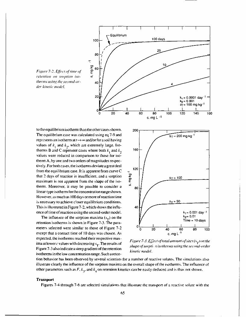
10 Equilibrium10 - . 100 days

80

" 60-Figutre 7-2. Effc 0)tie

re'tenftion on sorption iso- (1i

therms usin, the second-or- 40der kinetic model.

20 t/ k,: 0.0001 day"! / / /k2 = 0-001 .r t / ST= 100 mg kg-1

0 20 40 60 80 100 120 140 160c, mg L -1

to the equilibrium isotherm than the othercases shown. 200The equilibrium case was calculated using eq 7-9 and ST = 200 mg kgl

represents an isotherm at t-- oo and/or for a soil havingvalues of k, and k , which are extremely large. Iso-therms B and C represent cases where both kI and k 2 160

values were reduced in comparison to those for iso-therm A, by one and two orders of magnitudes respec-tively. For both cases, the isotherms deviate a great dealfrom the equilibrium case. It is apparent from curve C 17that 2 days of reaction is insufficient, and a sorption --Mo ST = 100

maximum is not apparent from the slape of the iso- Etherm. Moreover, it may be possible to consider a 80linear-type isotherm for the concentration range shown.However, as much as 100 days or more of reaction timeis necessary to achieve cOoser equilibrium conditions. ST 50

This is illustrated in Figure 7-2, which shows the influ- 40ence of time of reaction using the second-order model. k, 0.001 day-1

The influeice of the sorption maxima (sT) on the k2= 0.01

retention isotherms is shown in Figure 7-3. The para- 1ime1 1meters selected were similar to those of Figure 7-2 0 20 40 60 80 100except that a contact time of 10 days was chosen. As c, mg L-expected, the isotherms reached their respective max- Figure 7-3. Eet oftotalamountofsites(s oi theima at lower c values with decreasing sT. The results of

T' shape of sorpti. n isotheris using the second-or-derFigure 7-3 also indicate a steep gradient of the retention kinetic model.isotherms in the low concentration range. Such a reten-tion behavior has been observed by several scientists for a number of reactive solutes. The simulations alsoillustrate clearly the influence of the sorption maxima on the overall shape of the isotherms. The influence ofother parameters such as F, k3. and k4 on retention kinetics can be easily deduced and is thus not shown.

TransportFigures 7-4 through 7-6 are selected simulations that illustrate the transport of a reactive solute with the

65

second-order two-site (SOTS) model as the governing retention mechanism. The parameters selected for thesensitivity analysis were p = 1.25 g cm-3 L0cm.c =0.c = 10 m3. Li , F=0.50. and

sT = 200mg kg -. Here we assumed a solute pulse was applied to a fully water-saturated soil column initially

devoid of a particular heavy metal of interest. In addition, a steady water flow velocity (v) was maintainedconstant with a Peclet number P (= vL/OD) of 25. The length of the pulse was assumed to be 3 pore volumes.which was then followed by several pore volumes of a heavy-metal-free solution. The rate coefficients selectedwere 0.01,0. 1. 0.001. and 0.01 day-I for kI.k,. k . and k4. respectively. As a result, the equilibrium constantso) and o, for type I and 2 sites, respectively. were identical.

Figure 7-4 shows breakthrough curves (BTCs) that represent the relative effluent concentration (C/C0) vseffluent pore volume (1V/I) for several pulse input concentrations (C0 s). The shape of the BTCs is influencedby the input solute concentration and is due to the nonlinearity of the proposed second-order retention mech-anism. The simulated results also indicate that for high C values the BTCs appear less retarded and have sharp0gradients of the desorption (or right) side. In contrast, for low C. values the general shape of the BTCs appears

I I I I I I I I I

1.0

0.8 -/ - C0 = 1 mg L-1

120

C - 200500

0.4 -

0.2 /K

00 1 2 3 4 5 6 7 8 9 10

VN 0Fi'lur'e 7-4. Effliuent 'om'enti'iion distriltltivns or dierent initial concentratiins (c")utsing the se od-oder t0o-site (SOTS) inod'el.

1.0-ST =50 mg kg

0.8 -

0 0.6-10

0 1 2 3 4 5 6 7 8 9 10VNo

Figure 7-5. Effluent concentration distributirmsfinr different s.I. values utsiv,' the SOTSmodel.

66

1. / I I I I I I I I I /

0.8

0o0.6- v= 0.1 cm day1 -

/ ~ \10.4 4

0.2 -40 0" ,

0 1 2 3 4 5 6 7 8 9 10

VN 0

Figure 7-6. Effluent concentration distributionsJbr different flu. (v) values using theSOTS model.

to be kinetic. Specifically. as C decreases, a decrease in maximum or peak concentrations and extensive tailingof the desorption side of the BTCs can be observed. The influence of the total amount of (active) sites (sT )onthe BTCs is clearly illustrated by the cases given in Figure 7-5. Here the value of C was chosen constant (C= I0mg Li ). The BTCs show that an order of magnitude increase in sT (from 50 to 500 mg kg- ) resulted inan approximately 3-pore-volume shift in peak concentration. In addition, for high sT values extensive tailingas well as an overall decrease of effluent concentrations (C/C0) was observed.

The influence of the flow velocity (v) on the shape of the BTC is somewhat similar to that of the rate coef-ficients for retention, provided that the Peclet number remains constant. This is illustrated by the simulationsshown in Figure 7-6 for a wide range of flow velocities. For v = 40 cm day- the retention reactions associatedwith type I sites were not only dominant but also closer to local equilibrium than those for type 2 sites (resultsnot shown). This is a direct consequence of the limited solute residence time encountered when the fluid flowvelocity is exceedingly high. Type 2 sites that may be considered highly kinetic were so far removed from equi-librium that only a limited amount of solute was retained from the soil solution. Under such conditions, theamount of available sites (0,) remains high and the retention capacity of the soil matrix is therefore not achieved.In fact, curve A (v = 40 cm day- ) describes closely a one-site retention mechanism, as indicated by the low re-tardation and lack of tailing of the desorption side. As the flow velocity decreases, the solute residence time in-creases and more time is available for the highly kinetic type 2 sites to retain solute species from the soil solution.In addition, for extremely small velocities (v - 0) the BTC should indicate maximum solute retention duringtransport. This probably ,esembles the BTCs of curve E, which indicates the highest solute retardation shown.For intermediate velocities, however, the BTCs of B, C, and D indicate relatively moderate degrees of retard-ation as well as tailing that is indicative of kinetic retention mechanisms.

In the BTCs shown in Figures 7-4 through 7-6. the irreversible retention mechanism for heavy metal removal(via the sink term) was ignored. The influence of the irreversible kinetic reaction (e.g., precipitation) is astraightforward one, as shown in Figure 7-7. This is manifested by the lowering of solute concentration for theoverall BTC for increasing values of k,. Since a first-order reaction was assumed, the lowering of the BTC iss

proportional to the solution concentration.In previous BTCs. the sensitivity of model predictions (output) of the second-order approach to selected

parameters was discussed. It is convenient, however, to carry out model sensitivity using dimensionless para-meters such as those defined by eq 7-15 to 7-20. Dimensionless parameters offer a distinct advantage over con-ventional parameters since they provide a wide range of application as well as further insight into the predictivebehavior of the model. Figures 7-8 through 7-10 are simulations that illustrate the transport of a reactive solute

67

I I I I I I I I I

1.0

0.8 k =0 hr- 1

0 0.060.6 -

0.4 -

0.2

0 1 2 3 4 5 6 7 8 9 10V/Vo

Fig'ure 7-7. Effluent concentration distributions for values ol the irreversible rate co-efficient (ks) usin- the SOTS model.

I I

1.0- Q= 0.1

0.8 -

o 0.6

50.4 I

0.2 / 10

0 1 2 3 4 5 6 7 8 9 10V/V 0

Fgiure 7-8. Effluent concentration distributions for different values of parameter Q of theSOTS model.

with the SOTS model forselected dimensionless parameters. Unless otherwise indicated, the values fordimen-sionless parameters K2. K1, K 32 K 4' F. Ks P, and T were 5. 1, 1,O.1,0.1i,, 0.5, 25. and 1, respectively. Figure7-8 shows breakthrough curves (BTCs) of a reactive solute for several values of Q. The figure indicates thatthe shape of the BTCs is influenced drastically by the value of Q. This is largely due to the nonlinearity of theproposed second-order retention mechanism. As given by eq 7-24. K2 represents the ratio of total sites (sT ) toinput (pulse) solute concentration (Co). Therefore, for small !s (e.g.. Q =0.1), the simulated BTC is very similarto that for a nonretarded solute, due to the limited amount of sites (ST) in comparison to C . In contrast, largevalues of Q resulted in BTCs that indicate increased retention as manifested by the rightward shift of the peakconcentration of the BTCs. In addition, for high f s, extensive tailing as well as an overall decrease of effluentconcentration was observed.

The effect of the dimensionless reaction rate coefficients (K1. K."K and K4) of the two-site model on solute

68

K K K K

1.0 - 0.1 0.1 0.01 0.01-

1 1 0.1 0.1

0.8 - 10 0" 1-" 1 " 2

0.6 -

0.4 - /

0.2

0 ---0 1 2 3 4 5 6 7 8 9 10

V/Vo

Figure 7-9. Effluent concentration distriutions for differeint values otrate coefficients(K/, K2, K. and K4 ) using the SOTS model.

1.0

0.8

0 6 - F 0 1

0.4

0 1 2 3 4 5 6 7 8 9 10VN 0

Figure 7-I0. Effluent concentrationl distributions fw liffer-ent values of the fraction ofsites F using the SOTS model.

retention and transport is illustrated by the BTCs of Figure 7-9 where a range of rate coefficients differing bythree orders of magnitude was chosen. For the BTCs shown, the rate coefficients for type 2 sites were chosento be one order of magnitude smaller than those associated with type I sites. These BTCs indicate that, depend-ing on the values ofKi, K2.,K3. and K4.two extreme cases can be illustrated. For large K values, rapid sorption-desorption reactions occurred for both type I and type 2 sites. Rapid reactions indicate that the retention processis less kinetic and the BTCs can approximate local equilibrium conditions in a relatively short contact time(curves C and D). In contrast, for extremely small K values (or short residence time), little retention takes placeand the shape of the BTC resembles that for a nonreactive solute (curve A). The behavior of all illustrated BTCsis consistent with those for first-order kinetic and for two-site nonlinear equilibrium-kinetic reactions. Figure7-10 shows BTCs for several values of the fraction of sites parameter F. There are similar features between theBTCs of Figures 7-8 and 7-9 and those illustrated here. For F = I, all the sites are type I sites, which we desig-

69

nated earlier as those sites of strong kinetic influence due to their large values of K1 and K,. As the contributionof type 2 sites increases (or F decreases), the shapes of the BTCs become increasingly less kinetic with signif-icant decreases in amounts of solute retention.

SOTS COMPUTER PROGRAM

The computer code for the SOTS model is written in Fortran. Two versions are available: one is for use withmainframe computers and the other with personal computers. The input and output variables used in the SOTSmodel are given in Tables 7-1 and 7-2, respectively. The input data required for the SOTS model is given at theend of the code for the mainframe version. The appropriate values of model parameters must be provided bythe user in the input data section before the mainframe version is run.

A listing of the Fortran code for the PC version of the SOTS model (SOTSPC) is given in Appendix C. ThePC version allows the user to choose to enter the required model parameters in one of two ways: interactivelythrough the keyboard or by providing the name of an existing file that contains the input data. An example ofan input data file to be used with the PC version (SOTSPC.DAT) is included in Appendix C. The input para-meters listed were used for the sensitivity analysis presented in Figure 7-8. The PC version of SOTS was com-piled using a Fortran compiler, which results in an executable file (SOTSPC.EXE).

To use the compiled PC version of the SOTS model, the user need only type SOTSPC to run the program.You will then be prompted for the name and destination of an output file where all model calculations will bestored. If you choose to provide the input data interactively, you will also be prompted to enter the appropriateinput parameters in the order tiven in the data file. For convenience, default values for soil parameters andreaction rate coefficients are included. Forany parameter, the default value will be used if the userdoes not pro-

Table 7-1. List of input parameters required for the SOTS model.

Card Cohtnin 1VariahlenImbr ittlher format Iantie Definitilon

I 1-80 20A4 USER User s name or any other information (optional)

II 1-80 20A4 SOIL qoil name or any other infonnation (optional)111 1--80 20A4 SOLUTE Solute species orother information (optional)

VI 1-80 20A4 DATE Date. experiment number, or any other information (optional)

I 51-70 E20.6 TH Soil moisture content (8), cm cini

2 51-71) E20.6 ROU Soil bulk density (p). gcm

3 5I-7) E20.6 COL Thickness of ihe soil profile fL). cm

4 51-70 E20.6 WFLX Water flu.x ('. cm hr5 51-701 E20.6 CI Initial solute concentration in soil solution (C,). n L'6 51-71) E20.6 CS Concentration of applied solution (C 0 mg L7 51-70 E20.6 D Dispersion coefficient (D). cmI hr8 51-70 E20.6 ST Total sorption sites (c). mg kg '

9 51-70 E20.6 F Fraction of type I sites to total sites(F), dimensionless10 51-70 E20.6 K I Forward rate coefficient for type I sites (k1, hr 1

II 51-70 E20.6 K2 B.ckward rate coefficient for type I sites(A.,) h-12 5 1-, E20.6 K3 Forward rate coefficient for type 2 sites (k3). hr 1

13 51-70 E20.6 K4 Back% j."d rate coefficient for type 2 sites (k4), hr

14 51-7(0 E20.6 KS Irreversible rate coefficient (/1) (hr

15 51-53 13 IT Number of iterations to16 51-70) E20.6 TPULSE Duration of pulse (t ), hr

17 51-70) E20.6 TTOTAL Total simulation, hrI8 51-70 E20.6 TPRINT Time interval for printout, hr

19 51-70 E20.6 DX Initial gue, for the depth increment lail, cm

20 51-70 E20.6 DT Initial ltes, for the time shp (A), hr

70

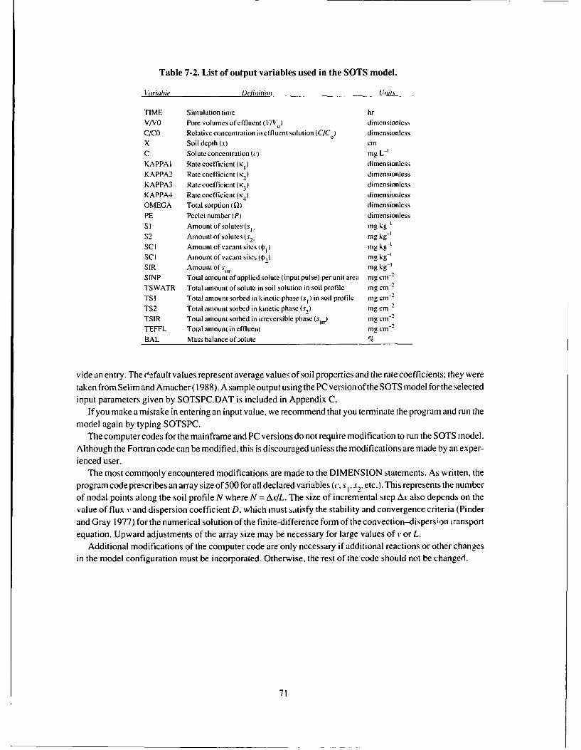
Table 7-2. List of output variables used in the SOTS model.

Variable Definition Units

TIME Simulation time hr

V/VO Pore volumes of effluent 0 71'o ) dimensionlessC/CO Relative concentration in effluent solution (C/C) dimensionlessX Soil depth (x) cmC Solute concentration (c) mg L-KAPPA I Rate coefficient (K) dimensionlessKAPPA2 Rate coefficient (K2) dimensionlessKAPPA3 Rate coefficient (K3 ) dimensionlessKAPPA4 Rate coefficient (K4) dimensionless

OMEGA Total sorption (Qi) dimensionlessPE Peclet number (P) dimensionless

SI Amount of solutes (s,, mg kg

S2 Amount of solutes (s, mg kg-SCI Amount of vacant sites (0 1) ing kg-SCI Amount of vacant sites (0,) mg kg-'

SIR Amount of s. mg kg'

SINP Total amount of applied solute (input pulse) per unit area mg cm-2

TSWATR Total amount of solute in soil solution in soil profile mg cm -2

TSI Total amount sorbed in kinetic phase (st ) in soil profile mg cm -

TS2 Total amount sorbed in kinetic phase (s,) mg cm -2

TSIR Total amount sorbed in irreversible phase (sin) mg cm-2

TEFFL Total amount in effluent mg cm-2

BAL Mass balance of 3olute %

vide an entry. The Oefault values represent average values of soil properties and the rate coefficients; they were

taken from Selim and Amacher (1988). A sample output using the PC version of the SOTS model for the selectedinput parameters given by SOTSPC.DAT is included in Appendix C.

If you make a mistake in entering an input value, we recommend that you terminate the program and run themodel again by typing SOTSPC.

The computer codes for the mainframe and PC versions do not require modification to run the SOTS model.Although the Fortran code can be modified, this is discouraged unless the modifications are made by an exper-ienced user.

The most commonly encountered modifications are made to the DIMENSION statements. As written, theprogram code prescribes an array size of 500 for all declared variables (c, sI, s2, etc.). This represents the numberof nodal points along the soil profile N where N = Ax/L. The size of incremental step Ax also depends on thevalue of flux v and dispersion coefficient D, which must satisfy the stability and convergence criteria (Pinderand Gray 1977) for the numerical solution of the finite-difference form of the convection-dispers;on transportequation. Upward adjustments of the array size may be necessary for large values of 1' or L.

Additional modifications of the computer code are only necessary if additional reactions or other changesin the model configuration must be incorporated. Otherwise, the rest of the code should not be changed.

71

Chapter 8. A Second-Order Mobile-Immobile Retention and Transport Model

InChapter 7. the second-order reactions associated with type I and 2 sites were considered as l.inetically con-

trolled, hete rogeneous, chemical retention reactions (Rubin 1983). One can assume that these processes are pre-dominantly controlled by surfacc reactions of adsorption and exchange. In this sense, the SOTS model is along

the sane lines as the earlier two-site model ofSelim et al. (1976) and Cameron and Klute (1977). Another type

of two-site model is that ofVillermaux ( 1974). which is capable of describing breakthrough curves (BTCS) from

chromatography columns with two concentration maxima.In this chapter. we invoke the second-orderconcept in a different manner. We consider that retention is con-

trolled by two types of reactions: namely a chemically controlled heterogeneous reaction and a physically con-

trolled reaction (Rubin 1983). In our analy : is we will consider the chemically controlled heterogeneous reactionto be governed according to the second-order approach. In the meantime, the physically controlled reaction willbe described by diffusion or mass transfer of the mobile-immobile concept (Coats and Smith 1964. van

Genuchten and Wierenga 1976). To utilize this concept, we assume 6" (cm 3 cm -3) as the mobile water contentthat is present inside large (inter-aggregate) pores where solute transport occurs by convection and dispersion.The immobile water Oil (cm 3 cn- 3) is located inside aggregate pores (intra-aggregate) where the solute transfer

occurs by diffusien only. c"' and ci" (mg L- 3) are heavy metal concentrations in the mobile and immobile phases,.respectively. In addition, the soil matrix is assumed to be divided into two regions or sites, namely a dynamicor easily accessible region and a less accessible region. The dynamic region is located close to the mobile waterphase, while the stagnant region is in contact with the immobile phase. Additional details on the assumptions

of the mobile-immobile (or two-region) approach are given in Coats and Smith (1964) and van Genuchten andWierenga (1976). It should also be mentioned here that analogies between the mobile-immobile concept andthe two-site approach can be made. One may regard the dynamic and stagnant regions for solute retentionanalogousto tye I and 2 sites of the two-site concept. Nkedi-Kizzaet al. ( 19 .) presented a (etailed discussionon the equivalence of the mobile-immobile and the equilibrium-kinetic two-site models.

MODEL FORMULATION

The form ofthe transport equation forthe mobile-immobile waterconcept can be written as (van Genuchten

and Wierenga 1976)

i)("' 1"/ t + p (I -f'" ))""t+ 0"' ")./II + pJ"' s'"lt

6111 D"' r)2(m'l)v 2 - , c'/x - Qn (8-I

where D"' is the hydrodynamic dispersion coefficient (cn 2 hr I ) in the mobile waler region, p is soil bulk density

(gcm- 1)., xis distance in the soil profile (cm), and i is time (hr). The associated transferequation governing theinteraction between solute in the mobile and immobile phases is

0'"' a ''''IrJt + p ( I -J 11) )s'"/dt = u.( (P1 - di n) - QI', (8-2)

where c. is the mass transfer coefficient (hr- ) between the mobile and immobile phases. In addition. .'." and .s""

(mng kg 1) are the sorbed amounts in the dynamic and stagnant regions. respectively. In eq 9- I and 9-2. the tenI ' (dimensionless) denotes the fraction of dynamic or active sites to the tolal sites .- (mg kg- ). This term is

analogous to F of the two-site model described in the previous chapter.In this model the terms d)s"'fri) and ).sY"/d)t represent the rates of reversible heavy metal reactions between

if] soil solution and that present on matrix surfaces in the mobile (or dynamoic) .i1(1 the imnmobile regions, re-

spectively. Moreover, irreversible reaction of heavy letals was incorporaled in this mlodel, as may eIt seen by

72

thle inclusion of the sink terms Q' and Q"" (mg cm- hr" ) in eq 8-1 and 8-2, respectively. We assumed thatirreversible retention or removal from solution will occur separately in the mobile and immobile water regions.However, the governing mechanism of retention for each region was assumed to follow first-order type reac-tions. Specifically, we propose that irreversible retention for the mobile and immobile regions be consideredin our transport model as follows:

Q= 11 k c (8-3)s

Qim = 1 1 ks -i'Y (8-4)

where k is the irreversible rate coefficient (hr ). The above formulations for the sink terms have not been seenelsewhere in the literature and were first proposed by Selim and Amacher( 1988). Since soil matrix surfaces maybehave in a separate manner to heavy metal retention, it is conceivable that the rate of irreversible reactions inthe mobile region could be characteristically different from that for the mobile region. One way to achieve thisis to distinguish between the rate coefficient (k ) controlling the reaction for the two regions, e.g.. k.. and k im

gst S Sin eq 8-3 and 8-4. respectively. Such a, distinction in reaction coefficients was not incorporated in our modeland a single parameter k was thus used.

The retention mechanism associated with the mobile and immobile phases of eq 8-I and 8-2 was consideredas an equilibrium linear sorption (van Genuchten and Wierenga 1976) and was extended to the nonlinear orFreundlich type by Rao et al. (1979). Recently, multiple-ion retention expressed on the basis of ion-exchangeequilibrium reactions was successfully incorporated into the mobile-immobile model (van Eijkeren and Loch1984. Selim et al. 1987). Here, we consider reversible solute reactions to be governed by our second-orderkinetic approach. Specifically, the rate of reaction fors.. and s"'1 were considered as (Sel im and Amacher 1988)

p as "I/t = O"'k1 1'1 c/' - p k, s"' (8-5)

p as I PIt 61i"'k, 01 ci - p (8-6)

where k and k, are the forward and backwyard rate coefficients (hr - ), respectively. Here 0. and 0ir representthe vacant or unfilled sites (nig kg - I ) within the dynamic and tile stagnant regions, respectively. In addition, theterms "' and ¢i" can be expressed as

In = "sTI -' n=f T - S (8-7)

N i T IM ., I_.i = (1 -f )ST _ sire (8-8)

where s T.ST. and s "" are the total amount of the sites in the soil matrix, total sites in the dynamic region. andthe total in the less accessible region (lig kg ). respectively. These terms are related by

'"T = 'Tm + 'Ti m =f"' ST +(I _J,)sT (8-9)

The unfilled sites 0"' and Owl are analogous to and 0, of the second-order two-site concept described in theprevious chapter. We also consider sT which represents the total amount of filled anu unfilled sites, to remaintime invariant.

An important feature of the second-order retention approach (eq 8-5 and 8-6) is that similar reaction rate coef-ficients (k1 and k,) associated with the dynamic and stagnant regions were chosen. It is assumed that the reten-tion mechanism is equally valid for the two regions of the porous media. A similar assumption was made byvan Genuchten and Wierenga (1976) for equilibrium linear and Freundlich-type reactions and by Selim et al.(1987) for selectivity coefficients for homovalent ion-exchange reactions. Specifically. as t - o. that is. whenboth the dynamic (or active) sites and the sites in the stagnant region achieve local equilibrium, eq 8-5 and

73

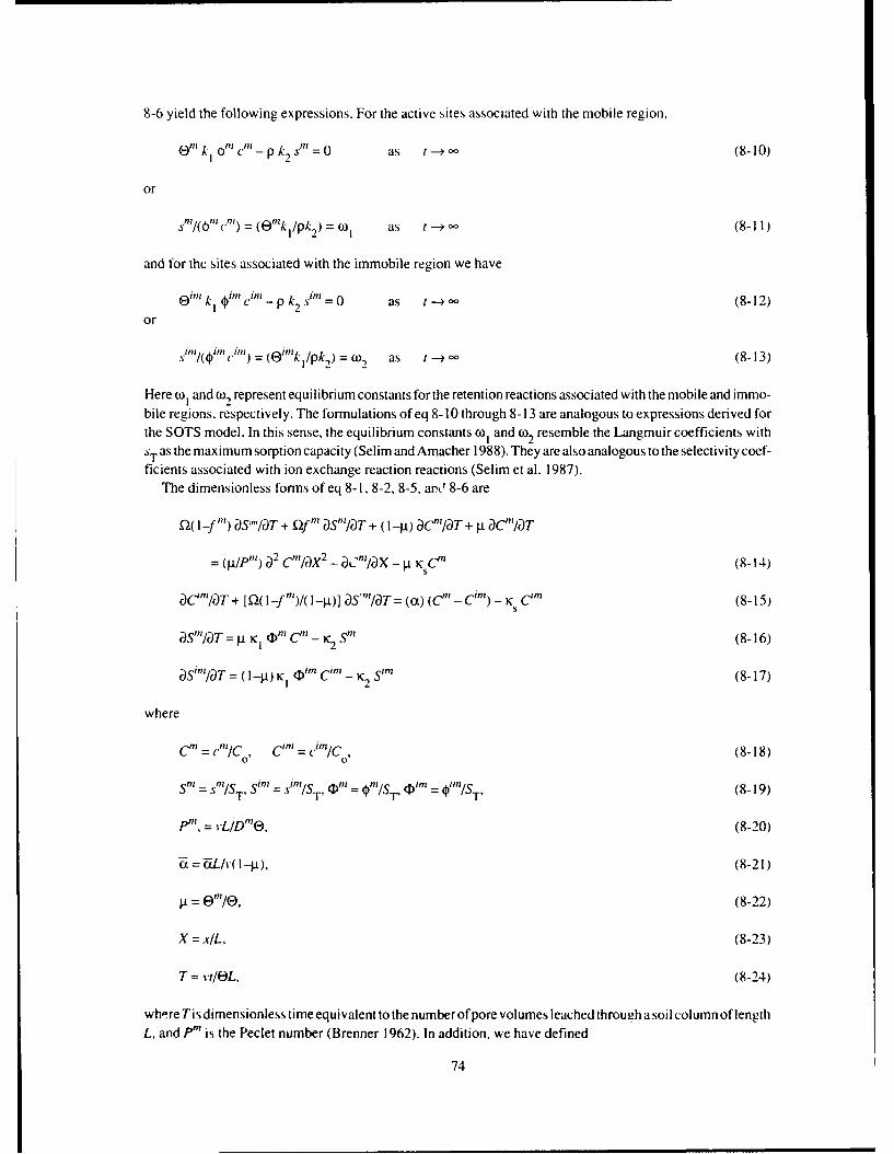
8-6 yield the following expressions. For the active sites associated with the mobile region,

On'k I on'cl-pk2 snz=o as t---, (8-10)

or

s'/(,"n c"n) = (O'nk/pk 2 ) = w as t--oc (8-11)

and for the sites associated with the immobile region we have

0in kl I ti _ p k2 s' = 0 as t c0 (8-12)or

sim[((it) = ((Ei'kI/pk2 ) = wl as t cc (8-13)

Here o and col represent equilibrium constants for the retention reactions associated with the mobile and immo-bile regions, respectively. The formulations of eq 8-10 through 8-13 are analogous to expressions derived forthe SOTS model. In this sense, the equilibrium constants 0) and (o2 resemble the Langmuir coefficients withsT as the maximum sorption capacity (Selim and Amacher 1988). They are also analogous to the selectivity coef-ficients associated with ion exchange reaction reactions (Selim et al. 1987).

The dimensionless forms of eq 8- 1. 8-2, 8-5, ant' 8-6 are

Q.( l-f n,) aSI''/T + Qf n, asn'/T + (I-_A) aCn'/aT + ;1 acn'/aT

= (,/p) a2 cnilax 2 _ -1.i'Dx _VK sCnm (8-14)

acm/aT + [f( l-f"')/( I-g.)] aS"'/T = (a) (Cn' - C) - K C'm (8-15)

aSi/lT= Pt K I (D ' Cn' - K 2 SM (8-16)

Sml/aT =(lI .) K (im CiR _ 'K2 Sir (8-17)

where

= *c C - /Co . (8-18)

S /S = SMIST, Sm" =S .l/ST , Dni = OmIST, (Dn=z i'm/ST , (8-19)

po, = vL/Dm.., (8-20)

c= .L/v( 1 -P), (8-21)

= e"'/E, (8-22)

X =x/L, (8-23)

T = vt/EL, (8-24)

where Tis dimensionless time equivalent to the numberof pore volumes leached through a soil column of lengthL, and Pm is the Peclet number (Brenner 1962). In addition, we have defined

74

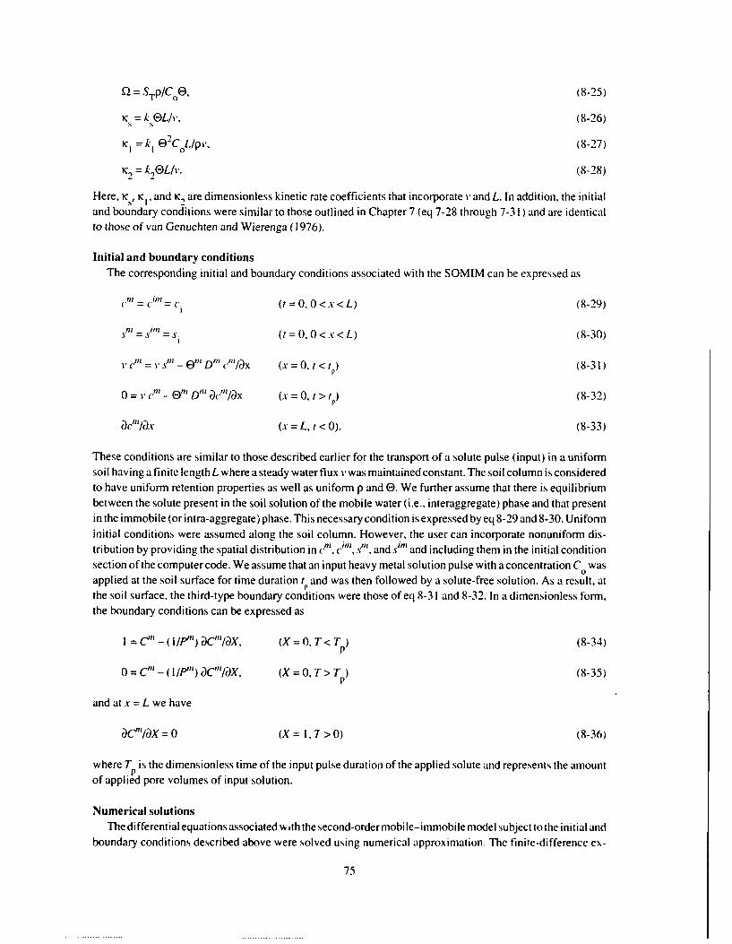
Q = STP/Co.9 (8-25)

K = k,8L/v, (8-26)

K,1 =k1 2CoL/Pv" (8-27)

K, = kEL/v. (8-28)

Here, K,, KI. and K, are dimensionless kinetic rate coefficients that incorporate v and L. In addition, the initialand boundary conditions were similar to those outlined in Chapter 7 (eq 7-28 through 7-31) and are identicalto those of van Genuchten and Wierenga (1976).

Initial and boundary conditionsThe corresponding initial and boundary conditions associated with the SOMIM can be expressed as

c"P = ini= c. (t = 0, 0 < x < L) (8-29)

SM =5 "m =s. (t=0,O<x<L) (8-30)

.cni = vs'n - "' D"' c/ax (x = 0. t < t) (8-31)

0 = v c"' - On' D'"' ac"'/3Jx (x = 0, t > t) (8-32)

acn/lax (x = L, t < 0). (8-33)

These conditions are similar to those described earlier for the transport of a solute pulse (input) in a uniformsoil having a finite length L where a steady water flux v'was maintained constant. The soil column is consideredto have uniform retention properties as well as uniform p and E. We further assume that there is equilibriumbetween the solute present in the soil solution of the mobile water (i.e., interaggregate) phase and that presentin the immobile (or intra-aggregate) phase. This necessary condition is expressed by eq 8-29 and 8-30. Uniforminitial conditions were assumed along the soil column. However, the user can incorporate nonuniform dis-tribution by providing the spatial distribution in c , Cira , ands and including them in the initial condition

section of the computer code. We assume that an input heavy metal solution pulse with a concentration C wasapplied at the soil surface for time duration t and was then followed by a solute-free solution. As a result, atthe soil surface, the third-type boundary conditions were those of eq 8-31 and 8-32. In a dimensionless form,the boundary conditions can be expressed as

I = CM -( IIPM) )C'/aX, (X = 0, T < T ) (8-34)

0 = Cm - (101) aC"'/aX, (X = 0, T > Tp) (8-35)

and at x = L we have

acnlaX = 0 (X= 1,7>0) (8-36)

where T is the dimensionless time of the input pulse duration of the applied solute and represents the amountof applied pore volumes of input solution.

Numerical solutionsThe differential equations associated with the second-order mobile-immobile model subject to the initial and

boundary conditions described above were solved using numerical approximation. The finite-difference ex-

75

plicit-implicit method (Remson al. 197 1, Pinder and Gray 1977) was used. Finite-difference solutions providedistributions of the dependent variables (e.g., solution and sorbed phase concentrations) at incremental dis-tances Ax and time steps At as desired. In a finite difference form a variable such as C is expressed as

C(x,t) = C(i A-, j At) (8-37)

where i=1,2,3.... N and j=1,2,3,... (8-38)

x = i Ax, and t =j At (8-39)

where N is the number of incremental distances in the soil (N = L/Ax). For simplicity, the concentration C(x,t)may be abbreviated as

C(x,t) = C.. (8-40)

where subscript i dti lotes incremental distance in the soil and superscriptj denotes the time step. We assumethat the concentration distribution at all incremental distances (A) is known for timej. We seek to obtain anumerical approximation ofthe concentration distribution at timej+ I ,j+2, and so on. The convection-dispersionequation along with the retention equations for reversible and irreversible reactions must first be expressed intheir finite difference approximation forms. Upon rearrangement and incorporation of the initial and boundaryconditions (in their finite difference forms), a solution is achieved. Details of the numerical scheme and the step-by-step derivation of the solution are provided in Chapter 3 and are similarto those of Selim and Iskandar (1980)for nitrogen transport.

The second-order mobile-immobile (SOMIM) model is solved in a sequential manner. Specifically, a solu-tion is obtained for each time step until the desired time for simulation is attained. It should be emphasized herethat the number of iterations, which are incorporated into the model to improve the accuracy of the solution atevery time step, for the above calculations must be provided by the user. No criteria are given here for the opti-mum number of iterations, rather a mass balance was performed (input vs output) as a check on the accuracyof the numerical solution. Therefore, the user is free to adjust the number of iterations based on mass balancecalculations or other criteria as desired.

SENSITIVITY ANALYSIS

Figures 8-1 through 8-5 are examples of simulated breakthrough curves (BTCs) to illustrate the sensitivityof the proposed second-order reaction, when incorporated into the mobile-immobile concept, to various modelparameters. As shown, several features of the mobile-immobile concept dominate the behavior of solutetransport and thus the shape of the simulated BTCs. For this reason we restrict our discussion to the influenceof parameters pertaining to the proposed second-order mechanism. Specifically, the influence ofk i and k2 (orKI and K 2 ) and w on solute retention were examined. Other parameters, such as D" and v, have been rigorouslyexamined in earlier studies (Coats and Smith 1964, van Genuchten and Wierenga 1976).

For the simulations shown in Figures 8-1 to 8-5, initial conditions, volume of input pulse, and model para-meters were identical to those used for the SOTS model, where c. = s. = 0 within the mobile and immobile re-gions. Sgecifically, the parameters chosen were L = 10 cm, Dm I cm 2 hr - 1 , p = 1.2 g cm- 3 f = 0.50. e =0.40 cm- cm =)"'/e= 0.5, co=100mgL s T = 200mg hr , anda Peclet number P"'= 25. Unless other-wise stated, the values selected for dimensionless parameters K, K2" K. fK , and a used were I, I. 0. 5, and I,respectively. We assumed a solute pulse was applied to a fully water-saturated soil column initially devoid ofa particular heavy metal of interest. In addition, a steady water flow velocity (v) was maintained constant witha Peclet number P of 25. The length of the pulse was assumed to be 3 pore volumes, which was then followedby several pore volumes of a heavy-metal-free solution.

76

I I I I I I I I

K I K 2

1.0- 0 0

0.01 0.0010.1 0.01

0.8 1 0.1

o0.6 -o /

A0.4 -

(X0.2 X

0-0 1 2 3 4 5 6 7 8 9 10

v/V o

Figure 8-1. Effluent concentration distributions for different values of K1 and K,using the SOMIM.

I I I I I I I |

K 1 K2 (0

1.0- 0 0 --1 1 0.015 1 0.02

0.8 - - 10 1 0.1

00.6-

0.4 -

/0.2 1- -

0 1 2 3 4 5 6 7 8V/Vo

Figure 8-2. Effluent concentration distributions for different values of

parameter 0) using the SOMIM. Values of Ki and K2 are also shown.

The influence of the reaction raie coefficients on the shape of the BTCs is illustrated in Figure 8- 1. Here thevalues of KI and K2 were varied simultaneously, provided that K 1/K2 (and o, and (0,) remained invariant. Forthe nonreactive case (K, = K, = 0), the highest effluent peak concentration and least tailing was observed. Asthe rate of reactions increased simultaneously. solute peak concentrations decreased and excessive tailing ofthe BTCs was observed. However, the arrival time or the location of peak concentration was not influenced byincreasing the rates of reactions.

The effect of increasing values of equilibrium constant o which represents the ratio of K,*, (see eq 7-9b.7- I Ob, 7-26, and 7-27). on the shape of the BTCs is shown in Figure 8-2. Here a constant value of I was chosenfor K,; K1 was allowed to vary. For all BTCs shown in Figure 8-2. the values of 01 and 0o, were equal (sinceS=0.5), so we refer simply to 0) rather than (o and o, The results indicate that as the forward rate of reaction

77

1.0a =2

0.8 1

02oQ 0.6 -/

0. 0.5 %0.4- ,jO 5

0.2 -

0 1 2 3 4 5 6 7 8 9 10VN 0

Figiure 8-3. Effluent concentration distributions for different values of the dimeli-

sionless mass transfer parameter d of'the SOMIM.

I I I

1.0-

.= 0.10.8

0 /5

90.6-/ 10

0.4 /

0.2-

I ~ -----

0 1 2 3 4 5 6 7 8 9 10VN 0

Figure 8-4. Effluent concentration distributions fir different values of parameter a ofthe

SOMIM.

(K1 ) increased, there was an increase in solute retardation ora rightward shift of the BTCs. This shift was accom-panied by an increase in solute retention (i.e., a decrease of the amount of solute in the effluent, based on thearea under the curve) and a lowering of peak concentrations. Similar behavior was observed for the influenceof the dimensionless transfer coefficient (a-) on the shape of the BTCs, as may be seen in Figure 8-3. For verylarge values of (>2), the diffusion between the mobile and immobile phases became more rapid. Therefore.equilibrium between the two phases is nearly attained (Valocchi 1985).

Figure 8-4 shows breakthrough curves (BTCs) of a reactive solute for several values of Q. The figure indi-cates that the shape of the BTCs is influenced drastically by the value of Q. This is largely due to the nonlinearityof the proposed second-order retention mechanism. As given by eq 8-25, Q represents the ratio of total sites (ST)to input (pulse) solute concentration (C0). Therefore, for small Us (e.g., Q = 0. 1), the simulated BTC is verysimilar to that for a nonretarded solute, due to the limited amount of sites (ST) in comparison to C . In contrast.

78

I I I I I I I I

1.0-

f fM 0.10.8 \ 0.25

~/O . /

0.2 - / 1.0 _v/o

Figiure 8-5. Effluent concentration distributions for different values of the faction of

active sites fm ofthe SOMIM.

large values of Q resulted in BTCs that indicate increased retention, as manifested by the right shift of peak con-

centration of the curves. In addition, for high i2s. extensive tailing as well as an overall decrease in effluent con-centration was observed.

The influence of parameterf"'. which represents the fraction of active or dynamic sites within the mobile

region to the total amount of sites on the behavior of solute retention and transport. is shown in Figure 8-5 for

several values off"'. There are similar features between these BTCs and those illustrated in the previous figures.Forf"' = 1. all the sites are active sites and thus there is no solute retention by the sites in the immobile region(that is, stagnant sites). As the contribution of the stagnant sites increases (orf"' decreases). the shapes of theBTCs become increasingly less kinetic with significant increase of the tailing of the desorption side of thecurves.

In the BTCs shown in Figures 8-1 through 8-5 the irreversible retention mechanism for heavy metal removal(via the sink term) was ignored. The influence of the irreversible kinetic reaction (such as precipitation) is a

straightforward one, so it is not shown. This is manifested by the lowering of solute concentration forthe overallBTC for increasing values of k . Since a first-order reaction was assumed, the lowering of the BTC is propor-

tional to the solution concentration. The influence of other parameters. such as P"' D"' and v. on the behaviorof solute in soils with the SOMIM have been studied elsewhere (van Genuchten and Weirenga 1976. Selim andMansell (1976) and are thus not examined here.

SOMIM COMPUTER PROGRAM

The computer code for the SOMIM is written in Fortran. It consists of a source (or main) program and twosubroutines, TRIDM and INTEG. The source program outlines the DIMENSION and COMMON statements.

the READ statements for the input parameters, the WRITE statements for the output data. and carries out theoverall step-by-step sequence of program calculations. In addition, it calculates the time steps and incremental

distances that satisfy the stability and convergence criteria (Pinder and Gray 1977) for the numerical solutionforeach given problem. All computations of the finite-difference approximations forthe convection-disperionequation and the retention equations and calculation of the coefficients needed for the set of equations at eachiteration and for each time step are also carried out in the source program. The input and output variables usedin the SOMIM are given in Tables 8-1 and 8-2. respectively.

79

Table 8-1. List of input parameters required for SOMIM.

CardI Colunin iariabhl'iinub'r numbewr b"orint t nanze /wowlini

1 -80 20A4 USER User's name or any other in fornation Ioptional,if 1-80 20A4 SOIL Soil name or any other inflorna, ion (optionah

111 1-80 20A4 SOLUTE Solute species or other inl onation (optional)VI 1-80 20A4 DATE Date. e.periment number, or any other in form ation (opt ional)

i 51-70 E20.6 TH Soil moisture content 1e). cmi cn2 51-70) E20.6 ROU Soil bulk density (p),. gcm3 51-7) E20.6 COL Thickness of soil prolile (L). cm4 51-70 E20.6 WFLX Water flux v), cm hr 15 51-70 E20.6 CI Initial solute concentration in soil solution (Cl, ing L6 51-70 E20.6 CS Concentration ofapplied solute solution (_ I),mg L7 51-70 E20.6 D Dispersion coefficient (D). cm 2 hr9 51-70 E20.6 ST Total sorption sites (s.,). mg kg 19 51-70 E20.6 F Fraction of sites in dynamic (or active sites in mobile) region to

total amount of sites f"), dimensionless10 51-70 E20.6 FTH Fraction of mobile water to total water content (e/6). dimensionlessII 51-70 E20.6 K I Forward rate coefficient (A ),. hr 1

12 51-70 E20.6 K2 Backward rate coefficient (1,. hr13 51-70 E20.6 KS Irreversible rate coefficient ( ). hri14 51-7(0 E20.6 TR Mass transfer coefficient (o, hr15 51-53 13 IT Number of iterations (r)16 51-70 E20.6 TPULSE Duration of pulse (t). hr17 51-70 E20.6 [TOTAL Total simulation, hr18 51-70 E20.6 TPRINT Time interval for printout. hr19 51-70 E20.6 DX Initial guess for depth increment (At), cm20 51-70 E20.6 DT Initial guess for time step (At). hr

Table 8-2. List of output variables used in SOMIM.

V "artahh' Definition Units

TIME Simulation time (t) hrV/VO Pore volume of effluent (1/1'd dimensionlessC/Co Relative concentration in effluent solution (C/C) dimensionlessX Soil depth (x) cmCM Solute concentration in the mobile region (.) mg L

CIM Solute concentration in the immobile region (c-) mg L

KAPPAI Rate coefficient w I ) dimensionlessKAPPA2 Rate coefficient (K) dimensionlessKAPPAS Rate coefficient (o.) dimensionlessTRANSC Rate coefficient lfi) Aim.nsi,,ilcssOMEGA Total sorption (Q) dimensionless

PE Peclet number iP) dimensionlessSM Amount of solutes sorbed in the active region (.s") mg kg

SIM Amount of solutes sorbed in the stagnant region I.%") mg kgSIR Amount of.s mg kg

rMW Total amount of solute in solution in mobile phase mg cmTSIMW Total amount of solute in solution in immobile phase mg cmTSM Total amount sorbed in active regioa I s) ol soil profile mg cm "TSIM Total amount sorbed in stagnant region s ''i ot soil profile mg cm -

TSIR Total amount sorbed in irreversible phase (.,) of soil profile mg cmiTEFL Total amount in effluent mg cm -

BAL Mass balance of solute ___,

80

Subroutine TRIDM provides a solution for a set of linear equations using the Thomas algorithm (Pinder andGray 1977) for tridiagonal matrix-vector equations. INTEG is an integration subroutine for equally spaced vari-ables: it is called by the source program to calculate the mass balance (input vs output) at specified times asdesired.

Two versions of the SOMIM are available: one is for use with mainframes and the other with personal com-

puters. The input section for the mainframe version is given at the end of the Fortran code. The user must adjust

the job-control cards according to the mainframe system to be utilized.A PC version of SOMIM is provided (SOMIMPC.FOR); it requires a Fortran compiler for personal com-

puters and includes an executable file named SOMIMPC.EXE. A computer listing of the Fortran code for thePC version is given in Appendix D. The PC version is interactive and allows the user to choose to enter the re-quired input data in one of two ways: interactively through the keyboard, or by providing the name of an existingfile that contains the input data. An example of an input data file to be used with the PC version (SOMIMPC.DAT)is included in Appendix D. The input parameters listed in SOMIMPC.DAT were used for the sensitivity analysispresented in Figure 8-2. A sample of the SOMIM output calculations for the input parameters given inSOMIMPC.DAT is included at the end of Appendix D.

To use the compiled SOMIM file, the user need only type SOMIMPC to run the program. You will then beprompted forthe name and destination of an output file where all model calculations will be stored. If you chooseto provide the input data interactively, you will also be prompted to enter the appropriate input parameters inthe order given in the data file. Forconvenience, default values for soil parameters and reaction rate coefficientsare included. The default value will be used for any parameter if you do not provide an entry. The default % aluesrepresent average values of soil properties and the rate coefficients; they were taken from Selim and Amacher(1988).

If you make a mistake in entering an input value, we recommend that you terminate the program and run themodel again by typing SOMIMPC.

The SOMIM computer codes do not require modification. Although the Fortran code can be modified, this

is discouraged unless the modifications are made by an experienced user.The most commonly encountered modifications are to the DIMENSION statements. As written, the program

code prescribes an array size of 500 for all declared variables (c' , c"', s", etc.). This represents the number ofnodal points along the soil profile N where N = &/L. The size of incremental step &r also depends on the valueof flux rand dispersion coefficient D, which must satisfy the stability and convergence criteria (Pinderand Gray1977) for the numerical solution of the finite-difference form of the convection-dispersion transport equation.Adjustments of the array size may be necessary for large values of vorL. Further modifications of the computercode are only necessary if additional reactions orotherchanges in the model configuration must be incorporated.

The remaining body of the code should not be changed.

81

Chapter 9. A Second-Order Retention Approach; Validation

We have presented a second-order kinetic approach for the description of solute retention during transportin soils. The basis for this approach is that it accounts for the sites on the soil matrix that are accessible for reten-tion of the reactive solutes in solution. This approach was incorporated with the fully kinetic two-site modelwhere the difference between the characteristics of the two types of sites is based on the rate of kinetic retentionreactions. We also assume that the retention mechanisms are site-specific, e.g., the sorbed phase on type I sitesmay be characteristically different in theirenergy of reaction and/or the solute species from that on type 2 sites.This approach, fully described in Chapter 7, was referred to as the second-order two-site (SOTS) model. InChapter 8, the second-order approach was extended to a diffusion-controlled mobile-immobile or two-regionmodel (SOMIM). In the SOMIM, we assume Em as the mobile water content that is present inside large (inter-aggregate) pores where solute transport occurs by convection and dispersion. The immobile water (E'"') islocated inside aggregate pores (intra-aggregate) where the solute transfer occurs by diffusion only. c"' and cm

are solute concentrations in the mobile and immobile phases, respectively. In addition, the soil matrix isassumed to be divided into two regions (orsites), namely a dynamic oreasily accessible region and a less access-ible region. The dynamic region is located close to the mobile water phase, and the stagnant region is in contactwith the immobile phase (for additional details see van Genuchten and Wierenga 1976). Analogies between themobile-immobile concept and that of the two-site approach can be made. One may regard the dynamic and stag-nant regions for solute retention as analogous to the type I and 2 sites of the two-site concept. Nkedi-Kizza etal. (1984) presented a detailed discussion on the equivalence of the mobile-immobile and the equilibrium-kinetictwo-site models.

A prerequisite for the validation of a model, such as the proposed SOTS model and the SOMIM, is that thenecessary (input) model parameters be obtained independently. In this chapter, model validations were carriedout using batch and miscible displacement data sets for Cr(VI) from three different soils. Furthermore, when-ever possible we used parameters that were either independently measured or estimated by indirect means.

EXPERIMENTAL

The soils used in this study are listed in Table 9-1 along with their taxonomic classification and selectedchemical properties. The soils were air-dried and passed through a 2-mm sieve before use. The retention ofCr(VI) by the soils was studied using the batch method outlined by Amacher et al. (1986, 1988). Initial con-centrations of Cr(VI) in the solutions reacted with the soils were 1, 2, 5, 10, 25, 50,75, and 100 mg L- 1. Back-ground solution composition for the Cr solutions was 0.005 M Ca(NO 3 )2 . A radionuclide tracer (7.4 x 106 BqL-1 5 1Cr ) was added to the Cr solutions tofollow the extent of the retention reac- Table 9-1. Taxonomic classification and selected chemicaltions. properties of the three soils.

The retention experiments were car-ried out as follows. Duplicate 4.0-g sam- Organicpies of each soil were added to preweighed Tavonomic matter CEC FeO

Soil classification pH ()(cmo1+ kg- I ('-/)

50-mL polypropylene centrifuge tubes. )

Then 40 mLofeach Cr solution wasadd- Cecil Clayey. kaolinitic, thermic 5.1 0.24 3.72 10.2ed to the duplicate samples of each soil, Typic Hapludults

and the samples were vortex-mixed. The Olivier Fine-silly, mixed, thermic 6.4 0.99 8.31 1.14tubes were placed endwise in a box on a AguicFragiudalfs

shaker set to shake at 120oscmin-.The Windsor Mixed,mesic 5.4 0.94 1.20 2.20samples were shaken for 15 min every 2 Typic Udipsamments

82

hr. After 2, 5. 8, 24.48, 72.96, 144, 192.240, 288, and 336 hr, the samples were centrifuged for 5 in at 1300x g, 20.0 mL of supernatant were withdrawn for counting the 320 keV 51 Cr peak by gamma spectrometry, thepH of the supernatants was measured, and the samples were reweighed. vortex-mixed, and returned to theshaker.

Concentrations of Cr in the sample solutions were calculated from the specific activities of the initial solu-tions and measured activities of the sample aliquots. Correction for radionuclide decay was avoided by countingthe initial solutions each time sample aliquots were counted. The amounts of Cr retained by the s,,s were cal-culated from the differences between the initial Cr concentrations in solution and the concentrations at each sam-pling time, with a correction for the amounts removed for counting.

The second-order two-site (SOTS) model was used to describe the retention data sets with a nonlinear, least-squares, parameter-optimization method (van Genuchten 1981). The criteria used for estimating goodness-of-fit of the model to the data were the r-square and the root mean square statistics. The extra sum of squares prin-ciple (Kinniburgh 1986) was used to detennine if there were any statistically significant improvement in thefit of the model to the data by adding more parameters (i.e., a two-reaction, three-parameter version vs a three-reaction, five-parameter version). Additional details are given in Chapter 4 and are also available in Selim andAmacher (1988).

Miscible displacement experiments were also performed to evaluate the SOTS and SOMIM models. Plexi-glas columns (4.4 cm in diameter x 6.35 cm long) were uniformly packed with each soil to a given bulk density(Table 9- I). Several pore volumes of 0.005 M Ca(NO 3 ), were introduced into each column at a constant flux(Table 9-1) to equilibrate the soils with the background solution. A pulse of radio-labeled 100 mg L- 1 Cr(VI)-0.005 M Ca(NO3)2 solution was introduced into each column at a constant flux, followed by several pore vol-umes of Cr-free background solution to elute the columns and obtain a complete breakthrough curve for eachsoil. A fraction collector was used to collect column effluent. The 320 keV 51 Cr tracer was counted using gammaspectrometry. To determine the dispersion coefficient (D) and the mass transfer coefficient (cc), a pulse of tri-tium (3 HI) and chloride-36 ( 6C1) was applied to each column prior to the Cr(VI) pulse. Liquid scintillationspectrometry was used to count the chloride-36 and tritium radiotracers.

KINETICS

Having formulated the model to include the total amount of sites or the retention capacity (sT) and the frac-tion of type I sites to the total amount of sites (F), some convenient method is needed to estimate their values.If the solute retention reactions with the two types of sites are reversible and reach equilibrium, then the rela-tionship between retained solute and solute remaining in solution can be described by the following two-siteLangmuir equation:

S/ 'v T F 1(1 Iec( I + ( Ic)] + ( I - F) (o.12 cl'( + (o, (-)1 (9-I )

where

s/sT = (sI + s,)/sT. (9-2)

Here sT represents the total retention capacity (mg kg - ) or the total number of sites onl matrix surfaces as timeinvariant. In addition. s I and s, (mg kg-[) are the amounts of solute retained (or the filled sites) on type I andtype 2 sites, respectively, and s (= s, + s,) is the total amount of solute retained (or the filled sites). Moreover.F represents the fraction of type I sites to the total amount of sites. Equation 9-I may be derived from the kineticsecond-order two-site concept, described in Chapter 7. when equilibrium conditions become dominant. Aspointed out by eq 7-9 and 7-10, whcn equilibrium conditions (t --+ ) are reached, we have

Ek, 0 1 c' - pk 2 s, =0 (9-3)

83

or

sl /(01 c) = (ek l lpk2) = (01 (9-4)

and for type 2 sites, we have

E k 3 q. c-p k4 s2 =0 (9-5)or

s,/(0(c)= (Ek 3/pk 4)= (9-6)

Here (o and to, represent equilibrium constants for the retention reactions, and and 0,2 are the numbers ofvacant sites associated with type 1 and type 2 sites, respectively. kI and k, (hr - ) are the forward and backwardrates of reaction for type I sites, while/"3 and k4 are the coefficients for type 2 reaction sites, respectively, Eis the soil water content (cm 3 cm-3), and p is the soil bulk density (g cm-3).

The two-site Langmuir equation was used to describe data for Cr(VI) retention by Cecil, Olivier, and Wind-sorsoils after 336 hrof reaction (Fig. 9- I, Table 9-2) using the nonlinear, least-sq u;res, parameter-optimizationsche &e of van Genuchten (1981). It was assumed that the reactions between Cr(VI) in solution and the two typesof sites had attained equilibrium in 336 hr even though small amounts of Cr(VI) were still being retained by thesoil. The continuing reaction between Cr(VI) in solution and the soil was ascribed to an irreversible reactionthat is included in the model (eq 7-14). The process responsible forthis irreversible reaction is discussed below.It is important to realize that only the reactions of Cr(VI) with the two types of reaction sites were assumed toattain equilibrium in 336 hr. Overall retention had not reached equilibrium because of the irreversible reaction.However, if the magnitude of the irreversible term is small, as is the case here, then reliable estimates of sT andF can! - made although the actual sT is somewhat smaller.

The statistical results from the parameter optimization scheme indicate a close approximation of the two-site Langmuir equation to the experimental sorption isotherms (Fig. 9-i and Table 9-2). However, a closeapproximation of the data does not constitute proof that two types of reaction sites actually exist (Sposito 1982).Parameter optimization merely provides a convenient method for estimating retention parameters given a pre-

1000 I I 500Time = 14 days

800 - 400

~Windsor7 600- 300

Ei 4 00 -0O livie r -2 0 0

200 1 00

100

0 40 80 120 160 200c, mg L-1

Figure 9-I. Chroniunn (V/) sorption isotherisfor Cecil. Windsor, and Oliviersoils after 14 days of reaction. The solid lines a'e calculated isotherms using the'equilibrium two-site Langimuir model.

84

Table 9-2. Maximum Cr retention capacity scribed model. Toour knowledge no reliable and independ-(s,, and fraction of sites (F) for three soils ent experimental method has been developed by which theusing equilibrium two-site Langmuir model. two types of reaction site,, can be distinguished unambigu-

ously and theirconcentrations accurately measured in soils.

Sol/ IN F),, F The time-dependent retention ofCr(VI) by Cecil. Oli vier.and Windsor soils was described using the SOTS model

Cccil 0J.9)90 5.51o 1127 ± 24 0.224 ± 0.I1 (Tables 9-3.9-4. 9-5: Figures 9-2.9-3.9-4). Two vrsionsOliicr 0.9)997 1.56 475 ± 1 .045 ± 10.1X)7 of the model were used: a three-paramneter or One-sile ver-WIin, 0.9J3 6.I 734 ±+ 41 (.)52 + ll9 sion (k I. ,. and k . in which T as not differentiated into

type I and type 2 sites (F = I ). and a five-paraleter or t\wo-Aite x ersion (k K, ,k " 4 and k) in which two types of reaction sites were considered. For most C s. either the

three- or five-piramleter versions described the data aidequately with high -square values and low parameter

standard errors. The exception was tile description of retention data for Olivier soil at high C where tile retentionof Cr! VI) was not hi-hlv kinetic and more scatter in experimental data points was observed.

For Windsor soil. the five-parameter model version provided the best description of' the data vt low Cwhereas the three-parameter model version was best for higher C .A significant improvement in model good-ness-of-fit was observed using the t5 ve-parameter version as compared to tile three-paramieter version at lowC values At hioh C no statistically signiticant improvement in goodness-of-fit could be obtained usine thefive-parameter version. Parameter values were often poorly defined with the five-paraimeter version at high C

0

indicating probable overfitting! of the data.

If the fraction of type I sites is small, as was the case with the Olivier and Windsor soils, then their contri-bution to the kinetic solute retention curve will be small and indistingu ishable at high solute concentrations. Forthe Cecil soil. where the fraction of type I sites was significant (22.4 ). the five-paraleter model version wassuperior to the three-parameter version at all C s except for C = I mg L-

. Therefore. the applicability of the0l o

five-parameter version to a widle rine of solute concentrations was directly related to the magnitude of the frac-

tion of type I sites. As F increased (Olivier < Windsor< Cecil). the concentration range increased, over whichthe five-parameter version provided a better description of the data than the three-parameter version.

The shapes of the experimental data curves and model calculations (Fig. 9-2.9-3. 9-4) are influenced by Co

At higher C ,retention ofCr( VI) froni solution was far less kinetic than at lower C .This behavior is as expectedif the concenltration of one or more reaction sites limits reaction rates. At C = 100 m- L - there wkere 4 mu ofCr(V11 available for reaction in a 40-mL solution volume. The maximumr possible amount of CR retention in4 g of soil \, as4.5. 1.9, and 2.9 mg (solute weight basis) forCecil. Olivier. and Windsor soils. respectively. Thus.,Maximum possibi. Cr retention in the Cecil soil was about equal to the ailount of Cr available for retention.Out was much less tlhaln the amount of Cr available for the Olivier and Windsor soils. Since the amount ot typeI sites was much I ss than the total. their contribution to the overall reaction is actually quite negligible at highsolute conc.,Litrit,ons. The influence of SlxC, or Q 1(Q = ST p/COE) A as defined when soluie retention durintransport was considered previously (see equation 7-24 and Figure 7-8).

The imagnitudes of the rate coefficients in Tables 9-3. 9-4. and 9-5 also depend oil . especially , h ,ichdecreases as C increases. Although thj iodel is successful in describing retentionl data for a given C( the same

rate coefficietits cannot be use( at substantially different C . It is doubtful thai ionic strength differences are ie-sp-nsible, since ionic st renigth varied only from O.015 to 0.01 . Differences in pH are also not likely to be re-,ponsible. since measured phi differences for all C s and at all reaction times were less than a 0.3 pLI unit. The,'ariation in rate coefficients with C mieht be attributed to chan-es in reaction miechanisls as C increased or

00

to failure to account for a. iit ,-tcom.,colllponents. Thus. tie SOTS nodei aiay not provide a complete descriptiotIof ill possible processe, that occur during retention. The mnodel is capable of describing tile time-uependence

of.,olute in solution. vacant sites, and solute-site complexes. However, only remosal of Cr1 Vb I r s)Ioil solu-

tioti was experimentally measured. For a complete K inetic rate lawe t ime-dependenc, of other react ion coni-potlents iust also be conside-ed such a. the species already on tie retent ion sites that were replaced by Cr ions.

Thus. this inodel ma be regiarded as an apparent rate law, rather than a mechanistic one.Although th. SOTS model can accurately describe experimetital data. lhis does not mean that it is tile correct

85

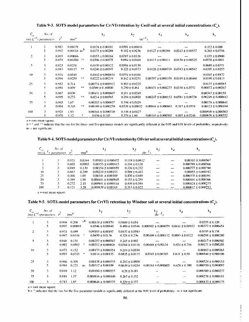
Table 9-3. SOTS model parameters for Cr(VI) retention by Cecil soil at several initial concentrations (C).

C', No. ,y k/ k2 k3 k4 ks

i ig, L po(ramters 2 I'llisa 1/-

I 3 0.983 0.00179 0.0128 ± 0.00101 0.0391 ± 0.00816 0- - (.322 ± 0.0865 (.992 0.001 18 nsb 0.0175 ± 0.00288 0.102 ± 0.0236 0.0127 ± 0.00388 1.0243 ± 0.00537 0.265 ± 0.0716

2 3 0.893 0.0(1686 0.0153 ± 0.00184 0.0387 ± 0.0126 - - 0.155 ± 0.09(X5 0.978 0.00310 0.0396 ± 0.(X1575 (1.094 ± (.01168 0.0113 ± 0.00111 0.0 150 0(1.011525 0.0530 ± 0.0891

5 3 0.923 0.0251 0.013(1 ± 0.00122 0.05(1 ± 0.0130 - - 0(1669 ± 0.03710.983 0.0117 0 0.0240 ± 0.00597 0.225 ± 0.0573 0.0128 ± 0.(X(X)719 0.0313 ± 0.00582 (1.0395 ± 0.0253

1M 3 0.971 0.0548 0.0102 ± 0.(XX1674 (.0554 ± 0.0104 - - 0.0345 ± 0.01725 0.994 0.0250 0.0222 ± 0.00219 0.142 ± 0.0231 0.(X)797 ± 0.(X)0339 0.0319 ± 0.00460 0.0199 ± 0.0113

25 3 0.952 0.314 0.(X1774 ± 0.(0912 01.103 ± 1.0225 -- 0.0 133±0. O.5835 0.994 0.119 10.0309 0 .005(X) 0.250 ± 0.464 0.00431 ± 0.000273 0.0530 + 0.0732 (.00872 ± 0.00267

5(t 3 0.967 0.83(0 0.0(431 ± 0.000607 0.111 ± 0.0249 - - 0.00347 ± 0.001555 0.995 0.273 0.0214 ±0.00565 0.294 ± 0.0820 0.00247 0.000153 0.0581 ±0.00736 0.M0249 ± (.000613

75 3 0.945 1.07 0.00555 ± 0.()0937 0.198 ± 0.0429 - -- 0.()178 ± 0.0X06415 (0.994 0.345 0.00180 0 (.01270 0.0338 ± 0.00652 0.00844 ± 0.000863 0.317 ± 0.0374 0.00123 ± 0(.000194

100 3 0,925 1.93 0.M(1344 ± 0.(1)(1730 0.148 ± 0.0427 0- - (.000940 ± 0.0005635 0.976 1.12 * 1.036 0.145 0.374 ± 1.60 O.(X) 193 +1000305 0.107 ±0.0246 0.001676 ± 0.000332

a =root mcean squtare.b = and indicate that tihe rins for the three- and live-parameter models are signilicantly different at the 0.05 and 0.01 levels of probability, respectively:ns = not signilicant.

Table 9-4. SOTS model parameters for Cr(VI) retention by Olivier soil at several initial concentrations (C).

C° No. I" f 2 ak I k-) k, k ks

-II I* ra r.I m a - (hr -J4

I 3 0.921 0.0344 0(.0(0113 ± 0.(10472 0.119 ± 0.(1612 - - 0.00103 ± 0.(X)5672 3 0.805 0.0803 0(.0(0155 ± 0.00(1915 0.194 ± 0.138 - - 0.000789 ± .01(X)5665 3 0.889 0.130 0.00 154 ± 0.()0959 0.326 ± 0.232 - - 0.000777 ± 0.(XX)?80

10 3 0.867 0.209 0.0)210 ± 0.00153 0.569 ± 0.483 I - 0.00055 ± 0.1(10192

25 3 0.406 1.119 0110141 ± 0.(X)189 0.470 ± 0.689 I - 0.000335 ± O.(XX)39150 3 0.389 1.98 0.000441 ± (.(00645 0.155 ± 0.259 - - 0.000101 ± 0.0(M)36675 3 0.272 2.15 0.00941 ± 0.(X)10144 0.410 ± 0.594 - - 0.(X)0124 ± 0.0(1233

100 3 0.121 3.20 0.000839 ± 0.(X)183 0.353 ± 0.822 - - 0.00()12 ± 0.(X)0253

.1 = root lleall square.

Table 9-5. SOTS model parameters for Cr(VI) retention by Windsor soil at several initial concentrations (C).

C o N,,. fk k, kak k4 ks

(n', L- I

)IIl,uailetc.s I Ms (h1

1 3 0.969 0.208 b (1.00119 ± 0.00170 0.0409 ± 0.154 - -0 0.0255 ± (1.1205 0.997 0.0(1694 0.0546 ± 0.1(1640 0.400 ± 0.0546 0.(10502 ± .01(XX)79 0.0411 ± 0.00933 0.00373 ± 0.01(M54

2 3 0.974 0.489 0.1X)103 ± 0.(X)197 0.0437 ± 0.0593 - - 0.0195 ± 0.1380.997 0.0144 0.0450 ± 0.0136 0.725 ± 0.236 0.(X)109 ± 0.(XX)112 0.0883 ± 0.0122 (.00298 ± 0.(X)0280

5 3 0.948 0.131 0.00257 ± 0.(X10767 0.245 ± 0.902 - - 0.0217 ± 0,0005025 0.992 0.0503 0.(X312 ± 0.000826 0.0384 ± 0.0116 0.00448 ± 0.()134 0.654 0 0.216 0.1X)171 ± 0.000205

10 3 0.973 0.152 0.00173 ± 0.(X)0351 0.219 ± 0.0559 0- - 0.00103 ± 0.0(X)2635 0.993 0.0745 10.0114 ± 0.(X)135 0.0835 ± 0.0115 0.0343 ± 0.00393 116.9 ± 0.59 0.(01844 ± 0.000106

25 3 0.966 0.309 0.(1138 ± 0.(1335 0.283 ± 0.0801) - - 0.(00524 ± 0.(01535 0.981 0.225 ns 0.(X0312 ± (.1(X) 1(1) 0.0639 ± 0.0254 (.1X) 184 0 (.010805 0.628 ± 0.3(M 0.1()0550 ± 0.(XXX)97

5(0 3 0.810 1.12 0.(X)100 ± 0.0(0555 0.28 ± 0.181 - - 0.000369 ± 0.010237

75 3 0.819 1.37 0.(X)0816 ±0.(XX)4(X) 0.267 ± 0.152 - - 0.(X)0278 ± O.(1 81

100 3 0.713 1.85 0.000648 ± 0.()0375 0.229 ± 0.157 - - 0.(X10133 ± O.(XX) 175

a = root ntcan square.b = * indicates that the rins for the five-paramcler models is significantly different al the 0.01 level of probability: ns = not signitican.

86

' ' ' iI C/Co 100mg'100 -= • l• • • 0

50

25

10 10-J

E Figure 9-2. Concentration of Cr2 vs time for a range of initial

1 1 concentrations (C () for Olivier

soil. The solid lines are calcula-

tions using the SOTS model.

0.1 IIIII

0 48 96 144 192 240 288 336Time, hr

100' C/Co =100 mg Ll

50

25

10 10

EFigure 9-3. Concentration of Cr

vs time for a range of initial2 concentrations (C )for Windsor

soil. The solid lines are calcula-1 tions using the SOTS model.

0.1 ..0 48 96 144 192 240 288 336

Time, hr

10 C1C0=' 100 mg 0-1

10 50

25

10

E 5 0 Figure 9-4. Concentration ofCr0 vs time for a range of initial

2 concentrations (Co ) for Cecil

0.01 1 soil. The solid lines are calcula-1 _tions using the SOTS model.

0.001 i

0 48 96 144 192 240 288 336Time, hr

87

or only explanation of the data. The model does not depend on any particular process of solute retention. Any

or all may be operative. including physical adsorption. formation of outer- or inner-sphere suiface complexes,

ion exchange. surface precipitation, etc. Furthermore, subsequent solute transfornations on the soil surface or

internal diffusion into soil particles may occur. Alternative processes may produce tile same experimental ob-

servations and many models may give similar results. This point was thoroughly discussed by Skopp (1986)

in his review of time-dependent processes in soils. Amacher and Selim (1987) and Amacher et al. (1988) found

that a nonlinear iultireaction model that does not include concentrations of reaction sites in its formulation can

describe tile experimental data as well as the SOTS model. Like the SOTS model, the nonlinear model is an in-

complete description of the actual reactions because the rate coefficients are dependent on C . Thus. b th types

of models yield pseudo rate coefficients.Physical and chemical processes that comprise reaction mechanisms occur at the molecular level, while ex-

perimental observations on soil systems are nearly always at the macroscopic level. Identification of chemical

species and reaction sites is necessary to distinguish among various possibilities, and such independent exper-imental evidence is for the most pait lacking in the case of reactions at soil surfaces. Greater progress has been

made in studying reactions at mineral surfaces (Davisand Hayes 1986). Sposito( 1986) indicated that when mul-

tiple retention mechanisms operate from the beginning of contact between solute and surface, as will likely be

the case in complex systems such as soils, then the time development of the overall retention process should

reflect this multiplicity of processes and defy simple interpretations based on simple models or nechanisms.

The pseudo rate coefficients reported here were obtained by parameter optimization because it is not yet

feasible to separate completely the reactions and determine their rate coefficients independently of each otherin systems as complex as soils. Furthernore. no simple single reaction model was found to describe adequately

the time-dependent data (Amacher etal. 1986). If a multireaction model does not adequately describe the data

it can be discarded, but even if it does describe the data it has limited predictive and explanatory capability until

independent supportive or contradictive evidence can be obtained. Despite these difficulties some limited

mechanistic interpretation of the model's description of the data can be given. The retention of solute by thevarious types of reaction sites is postulated to be formation ofouter-sphere and inner-sphere surface complexes.

Such possible surface reactions are known to occur and further discussion can be found in Davis and Hayes(1986) and Sposito (1984) among other references.

Inclusion of an irreversible reaction in the model is strongly suppoited by the continuing reaction betweenCr(VI) and the soils even after 336 hr. by the fact that overall retention was only partly reversible, and by thefact that little retained Cr could be replaced by phosphate ions (Amnacher et al. 1986). A first-order irreversible

reaction was chosen because at longer times and for a given Co . retention of Cr(VI) appeared to follow first-

order kinetics. The process responsible for this irreversible reaction is postulated to be reduction of Cr(VI) to

Cr(lll) with possible precipitation of Cr(III) on mineral surfaces or as discrete particles of hydrous Cr(lll)oxides. Oiganic matter. Fe(ll) minerals, and other possible reducing agents are known to irreversibly reduce

Cr(VI) to Cr(iill). Reduction of Cr(VI) to Cr(1II) by organic matter is a slow process at normal environmentalpH and temperature levels such as those used in this study (Baitlett and Kimble 1976: Bartlett and James 1979:Amacher and Baker 1982: James and Bartlett 1983a.b.c) and follows first-order kinetics if pH is constant(Amacher and Baker 1982). The overall reaction rate is pH-dependent (Amacher and Baker 1982). The irre-versible tern in the model (eq 7-14) is fully consistent with these observations. Since k is dependent on C . theS 0

irreversible reaction is more complex than a simple first-order reaction. At higher C,. amounts of reducing

agents may be limitingt and thus produce the observed dependence of k on C Thus. at a given C the reductionreaction is pseudo first-order.

Mendoza and Barrow (1987) proposed that the continuing reaction between phosphate ions and soils is the

penetration of adsorbed phosphate into the adsorbing surface. Aringhieri et al. (1985) proposed an internaldiffusion process toexplain why a single second-order reversible reaction failed to describe Cu and Cd retention

kinetics. As an alternative to the reductive sorption mechanism, this internal diffusion mechanism may alsoaccount for part of the continuing reaction between Cr(VI) and soils. Diffusion of Cr(VI) ions into soil particles

may partly explain why Cr(VI) retention is only partly reversible and retained Cr cannot be fully replaced by

phosphate ions. The internal diffusion process can be accounted for by the irreversible term in the model.

88

SOTS MODEL VALIDATION

Chromium BTCs from the miscible displacement experiments for all three soils are shown in Figure 9-5.For Cecil and Windsor soils the measured BTCs appear to be highly kinetic, with extensive tailing. For Oliviersoil little tailing was observed and approximately 100% of the applied Cr(VI) pulse was recovered. These resultsare consistent with the batch data, where ks was found to be quite small.

To examine the capability of the second-ordertwo-site (SOTS) model, the necessary model parameters mustbe provided. In this study we will attempt to utilize, whenever possible, parameters that are either independentlymeasured or estimated by indirect means. We will rely on parameter estimates from the batch studies discussedabove for the kinetic rate coefficients, fraction of sites, and total amount of retention sites foreach soil. Thesebatch parameters were used in conjunction with the SOTS model to describe the Cr(VI) BTCs shown in Figure9-5.

Values for the dispersion coefficients (D) were obtained from BTCs of the tracer data for tritium (3H.0)and chloride-36 (36C1) (see Table 9-6). These BTCs (figures not shown) were interpreted by use of the classi-cal convective-dispersive equation with a retardation factorR (R = I + pKd/e) where Kd is the Freundlich distri-bution coefficient (cm3 g- ). Best-fit model parameters forD (and R) were obtained by use of the nonlinear least-squares optimization method of van Genuchten (1981). It should be noted here that R values for the two tracersand all three soils ranged from 0.93 to 1.07, and little tailing of the BTCs was observed. Other model parameterssuch as p, 19, and v for each soil column are also given in Table 9-6. In addition, the values for sT and F usedto describe Cr BTCs from the SOTS model were those obtained using batch dataof the sorption isotherms shownin Figure 9-2 (see Table 9- I). Direct measurements of these parameters by other than parameter optimizationtechniques is not available. Moreover, we utilized the reaction rate coefficients k1, k2 ,k3, k4, and k. (Tables 9-3,9-4, and 9-5) as obtained from the batch kinetic data in the predictions ofCr BTCs. In the following discussion,predicted curves imply the use of independently measured parameters in model calculations as was carried outhere using the batch parameters.

The predicted BTCs shown in Figure 9-5 were obtained using different sets of parameter values for the ratecoefficients (k, k2, k3 ,k 4 , and ks) for the SOTS model. This is because no single or unique set of values for theserate coefficients was obtained from the batch data; rather a strong dependence of rate coefficients on inputconcentration was observed (see Tables 9-3 through 9-5). Forall the soils, several features of the predicted BTCsare similar and indicate strong dependence on the set of rate coefficients used in model calculations. Increasedsorption during transport, lowering of peak concentrations, and increased tailing were predicted when batch ratecoefficients from low initial concentrations (CO) were used.

The use of batch rate coefficients at C = 100mg L (which is the concentration of Cr pulse inputs) grossly0

underestimated Cr retention by the predicted BTCs for all soils (Figure 9-5). Reasons for this failure, which hasbeen observed by other scientists, are not fully understood. The most likely explanation is that the model is anapparent rather than mechanistic rate law as previously discussed because it may not completely account forall reactions and reaction components. Rate coefficients based on batch experiments varied with C , whichwould be expected of pseudo rate coefficients. Unless the concentrations of unaccounted-for reactioncomponents remain relatively constant over the course of thz experiment, rate coefficients will vary with C.because they implicitly include concentrations of other reaction components. Much larger changes wereobserved in Cr concentrations in column effluent (pulse input) than in the batch solutions. Although k, k2 . k3.and k were constant over a limited concentration range in the batch experiment, they did vary over a wide con-centration range. Thus, a valid set of rate coefficients from the batch experiment is not readily available to coverthe range of concentrations found in the miscible displacement experiment because of the concentrationdependence of the rate coefficients. This is particularly true fork which varied systematically with Co. Criteriafor choosing rate coefficients are needed in such cases.

For Olivier soil, predicted BTCs using the SOTS model indicate that the batch rate coefficients from a Cof either 10 or 25 mg L- provided ,urprisingly good overall descriptions of the experimental results. Less thanadequate predictions were obtained for the highly kinetic Cecil and W indsor soils, however. in fact, no one setof batch rate coefficients successfully described both the effluent and the desorption sides of Windsor or Cecil

89

1.0- 1

0.8- A

0 0.6 B a. Olivier soil. C/C of curves A-E

--CI are 100.25, 10, 5, and I mg L- ,IT0.4- spectively.

0.2- 0O o l

VNOI II I I I

1.0-

0.8- 0|

S0.6

B D b. Windsor soil. C/C of cun'es A-EC0. are25, 10,5,2,andl mg L-

, respec-tively.

0.2

0) 4 5v/vVNO

1.0

0.8-

A

0.6-

o / c. Cecil soil. C/C of curies A-D are

0.4- 100, 50, 25, and 10 mg L-, respec-0.4 -- /] - tively.

I. °O0.2-

Di i I ... I I

o 4 8 12 16 20 24 28 32VNo

Figure 9-5. Effluent concentration distributions for Cr predicted using the SOTS model with the hatch ratecoefficients indicated.

90

Table 9-6. Soil physical parameters for Cr BTCs. For both soils, closest predictions were realizedmiscible displacement experiments used with using batch rate coefficients from C of 10 or 25 mg L-I.the SOTS model and the SOMIM. This finding is similar to that based on the predictions

Paraneer Olivier Windsor Cecil for Olivier soil.

p (g cm - 3) 1.27 1.65 1.08

0 (cm 3 cm -3) 0.520 0.377 0.590 SOMIM VALIDATION

' (cm hr- 1) 0.14 0.17 0.13

D (cm2 hr-') 0.054 0.297 0.172 The capability of the second-order mobile-immobile(from CI-36) model (SOMIM) to describe Cr miscible displacement

D (cm2 hr- 1) 0.077 0.186 0.173 results was also examined; the predictions are shown in(from tritium) Figure 9-6. To obtain the predicted BTCs shown, sev-

D" (cm2 hr 1) 0.039 0.208 0.151 eral assumptions were necessary to estimate the model

a(hr-') 0.0758 0.0407 0.0271 parameters. A list of parameters used in conjunctionwith the SOMIM are given in Table 9-6. Values forsT

9"1/8 0.73 0.80 0.66 Lwere those determined from the sorption isotherms ofFigure 9-1 and Table 9-2. The ratio of mobile to total

watercontent (We8) for each soil was estimated based on soil-moisture retention relations for each soil (resultsnot shown). We also assumed that the fraction of sitesf"' is the same as the relative amount of water in the tworegions. i.e.. f"' = 0"'/E). Such an assumption was made because independent measurement off"' is notavailable (van Genuchten and Dalton 1986). Selim et al. (1987) successfully used such estimates off"' for awell-aggregated soil. Estimates for a were obtained using

at= 15 D a E( l-it)/a 2 (9-7)

where i = e" ieand D is the molecular diffusion coefficient in a soil consisting of uniform aggregates of radiusa. The above equation was derived by Parker and Valocchi (1986) and is based on time-moment an-ysis forspherical diffusion and for first-order kinetic (mobile-immobile) models. Our estimates for x are bas j on theassumption of average aggregate sizes of 0.01, 0.01, and 0.005 cm for Windsor, Olivier, and Cecil soils, re-spectively. In addition, Da for Cr diffusion was assumed to be 10-9 cm 2 s-1 for all three soils. Barber (1984)compiled diffusion coefficients fora number of ions in soils with values for phosphate (H2PO 4-) ranging from10-8 to 1 0- cm 2 s-I (for water Da = 0- cm 2 s-I). These values ofDa and gI were also used to estimate the hydro-dynamic dispersion coefficient (Dn') in the mobile-water region using (Parker and Valocchi 1986. eq 46)

Dn = (l/It) [D - (I-g) a2 v2/15 D"] (9-8)

where v is the pore water velocity (n/Ere). Values for the dispersion coefficient D used in the above equationwere averages of those obtained from BTCs of tritium and chloride-36 tracers. We should mention that attempts

to use 3H20 and 36CI BTCs for parameter estimation of aX and D"' were not successful. Values obtained usingthe optimization method of van Genuchten (198 1) were inconsistent and ill-defined due to large parameter stan-dard errors and were often physically unrealistic (e.g.. R >> ). Perhaps these results are due to local equilibriumconditions between the mobile and immobile regions for the two tracers (Rubin 1983. Parker and Valocchi1986). Tailing of BTCs was not observed from the tracer results.

Values for the rate coefficients used in the SOMIM were those calculated from the batch kinetic results. Spe-cifically, we used the k,, k2, and ks values given in Tables 9-3 through 9-5 obtained from the three-parameterversion of the second-order two-site model as described in Chapter 7. Predicted BTCs were obtained using dif-ferent sets of batch rate coefficients due to their strong dependence on input concentrations (Cos). The closestpredictions to experimental Cr measurements were obtained from batch rate coefficients at low C values (C1 0S 10 mg L ). Moreover. the use of rate coefficients at higher Cos resulted in decreased tailing and reducedretardation of the BTCs.

91

1.0A

0.8- B/'

S0.6 t

0.4-/ a.Olivier soil. C/C of curves A-D/0are 25.10,5, and 1(mg L1', respec-

0.2 - tively.

00

0 1 2 3 4 5 6 7 8VNO

1.0-

0.8-

~?0.6-

0.4- b. Windsor soil. C/C ofcurvesA-D

are 25, 5, 2, and 1 mg U7 respec-0.2- tively.

0

V/Va

1.0 T

0.8 -

0.6 -

0

0.c- CCecilsoil. C/C ofcurves A-C are

it 0 Go go25, 10. and 5 mg Us' respectively.

0.2 -

C.0 4 8 12 16 20 24 28 32

V/V0

Figure 9-6. Effluent concentration distributions for Cr predicted using the SOMIMA-ith the batch rate coef-ficients indicated.

92

These observations are consistent with previous predictions using the SOTS model (Fig. 9-5). However.overall predictions of measured Cr using the SOMIM is considered less than adequate in comparison to SOTSmodel predictions. Reasons for the less-than-adequate predictions of BTCs for the three soils using the SOM IMare not fully understood. It is conceivable that a set of applicable rate coefficients over the concentration rangefor Cr transport experiments cannot be obtained simply by use of the baich procedure described in this study.In addition. several parameters used in model calculations were estimated and not measured. e.g.. "'. ox. andD"'. The fractioii of actie sitesf"' was not estimated, rather it was assumed equal to tile mobile water fractioni®',iQ since iio means of its direct measurement was available. It is likely that improved BTC predictions couldbe obtained by use of parameter optimization. but such attempts were not pe,'forned. Other possible factors re-sponsible for these predictions may be due in part to lack of nonequilibrium conditions between the mobile and

immobile fiactions for the SOMIM (Valocchi 1985. Parker and Valocchi 1986).Based on the above analysis. we demonstrated the capability of a proposed second-order two-site (SOTS)

model to describe Cr(VI) kinetic (batch) behavior in three soils. Reaction., that were postulated to account forthe observed kinetic behavior include formation of surface complexes between Cr(VI) and soil. reductive sorp-tion or precipitation ofCr( VI). and internal diffusion. Moreover. tle SOTS model was partly successful in pre-d icti ng Cr miscible displacement results. The necessary model parameters. such as total amount of sites. fractionof sites. and rate coefficients, were not obtained by curve fitting, but were detemined independently. A uniqueset of batch rate coefficients capable of predicting the BTCs were not obtained due to their strong dependenceon input concentrations. When the proposed second-order approach was extended to the mobile-immobile(two-region) concept (SOMIM). little improvement in BTC predictions was achieved. The failure of themobile-immobile model was attributed to the estimates for the model parameters and/or lack of nonequilibriumconditions in these soils. Additional validation of the SOMIM is needed.

93

References

Alberts, J.J., J.E. Schindler, R.W. Miller, and D.E. Nutter, Jr. (1974) Elemental mercury evolution nedi-ated by humic acid. Science, 184: 895-897.Alesii, B. A., W.H. Fuller, and M.V. Boyle (1980) Effect of leachate flow rate in metal migration through soils.Journal of Environmental Quality, 9: 119-126.Amacher, M.C. and D.E. Baker (1982) Redox reactions involving chromium, plutonium, and manganese insoils. DOE/DP/04515-1. U.S. Department of Energy, Las Vegas. Nev. University Park, Pennsylvania: Institutefor Research on Land and Water Resources, Pennsylvania State University.Amacher, M.C. and H.M. Selim (1987) Prediction of reactive solute transport using nonlinear and second-order kinetic models. In Proceedings of the International Conference on the Impact of Physico-Chemistr) onthe Study, Design and Optinization of Processes in Natural Porous Media, Nancy, France, p. 95-103.Amacher, M.C.,J. Kotuby-Amacher, H.M. Selim, and I.K. Iskandar (1986) Retention and release of metalsby soils--evauation of several models. Geoderma, 38: 131-154.Amacher, M.C., H.M. Selim, and I.K. Iskandar (1988) Kinetics of chromium (VI) and cadmium retentionin soils, a nonlinear multireaction model. Soil Science Society of America Journal, 52: 398-408.Amoozegar-Fard, A., A.W. Warrick, and W.H. Fuller (1983) A simplified model for solute movementthrough soils. Soil Science Society of America Journal, 47: 1047-1049.Amoozegar-Fard, A., W.H. Fuller, and A.W. Warrick (1984) An approach to predicting the movement ofselected polluting metals in soils. Journal of Environmental Quality, 13: 290-297.Anderson, J. U. (1963) An improved pretreatment for mineralogical analysis of samples containing organic

matter. Clays and Clay Minerals, 10: 380-388.Anderson, W. L. and K.E. Smith (1977) Dynamics of mercury at coal-fired power plant and adjacent coolinglake. Environnental Science and Technology, 11: 75-80.Aringhieri, R., P. Carrai, and G. Petruzzelli (1985) Kinetics of Cu and Cd adsorption by an Italian soil. SoilScience, 139: 197-204.Avotins, P. and E.A. Jenne (1975) The time stability of dissolved mercury in water samples. II. Chemical sta-bilization. Journal of Environmental Quality, 4: 515-519.Barber, S.A. (1984) Soil Nutrient Bioavailibilitv; A Mechanistic Approach. New York: Wiley-Interscience.Bartlett, R.J. and J.M. Kimble (1976) Behavior of chromium in soils. II. Hexavalent forms.,Journal of Envi-ronmental Quality, 5: 383-386.Bartlett, R.J. and B. James (1979) Behavior of chromium in soils. III. Oxidation. Journal of EnvironmentalQuality, 8: 31-35.Brenner, H. (1962) The diffusion model of longitudinal mixing in beds of finite length; numerical values.Chemical Engineering Science, 17: 220-243.Buchter, B., B. Davidoff, M.C. Amacher, C. Hinz, I.K. Iskandar and H.M. Selim (1989) Correlation ofFreundlich K. and n retention parameters with soils and elements. Soil Science, 148: 370-379.Cameron, D. and A. Klute (1977) Convective-dispersive solute transport with chemical equilibrium andkinetic adsorption model. Water Resources Research, 13: 183-188.Carnahan, P., H. Luther and J.0. Wilkes (1969)Applied Numerical Methods. New York: Wiley.Cederberg, G.A., R.L. Street and J.0. Leckie (1985) A groundwater mass transport and equilibrium chem-istry model for multicomponent systems. Water Resources Research, 21:1095-1104.Chao, T.T. and L. Zhou (1983) Extraction techniques for selective dissolution of amorphous iron oxides fromsoils and sediments. Soil Science Society of America Journal, 47: 225-232.Coats, K.H. and B.D. Smith (1964) Dead-end pore volume and dispersion in porous media. Society of Petro-leum Engineering Journal, 4: 73-84.Cranston, R.E. and D.E. Buckley (1972) Mercury pathways in a river and estuary. EnvironmentaIScience andTechnology, 6: 274-278.Crecelius, E.A., M.H. Bothner, and R. Carpenter (1975) Geochemistries of arsenic, antimony. mercury. andrelated elements in sediments of Puget Sound. Environmental Science and Technology, 9: 325-333.

94

Daniel, C. and F.S. Wood (1973) Fitting Equations to Data. New York: Wiley-Interscience.Davis, J.A. and K.F. Hayes (Ed.) (1986) Geochemical processes at mineral surfaces. ACS Symposium Series323. Washington. D.C.: American Chemical Society.De Camargo, O.A., J.W. Biggar and D.R. Nielsen (1979) Transport of inorganic phosphorus in an Alfisol.Soil Science Society ojAinerica Journal. 43: 884-890.Dowdy, R.H. and V.V. Volk (1983) Movement of heavy metals in soils. Chapter 15 in Chemical Mobility andReactivity in Soil Systems (D.W. Nelson, Ed.). Soil Science Society of America (SSSA) Special Publication II.Madison, Wisconsin: American Society of Agronomy. p. 229-240.Dowdy, R.H., J.A. Ryan, V.V. Volk and D.E. Baker (Ed.) (1981) Chemistry in the soil environment. ASASpecial Publication 40. Madison. Wisconsin: American Society of Agronomy.Eganhouse, R.P., D.R. Young and J. N. Johnson (1978) Geochemistry of mercury in Palos Verdes sediments.Environmental Science and Technology. 12: 115 1-1157.Ellis, B.G., B.D. Knezek and L.W. Jacobs (1983) The movement of micronutrients in soils. Chapter 8 inChemical Mobility andReactivity in Soil Systems (D.W. Nelson, Ed.). Soil Science Society of America (SSSA)Special Publication 11. Madison, Wisconsin: American Society of Agronomy. p. 109-122.Elprince, A.M. and G. Sposito (1981) Thermodynamic derivation of equations of the Langmuir type for ionequilibria in soils. Soil Science Societv of America Journal, 45: 277-282.Elrashidi, M.A. and G.A. O'Connor (I 982a) Boron sorption and desorption in soils. Soil Science Society ofAmerica Journal. 46: 27-3 1.Elrashidi, M.A. and G.A. O'Connor (I 982b) Influence of solution composition on sorption of zinc by soils.Soil Science Society of America Journal, 46:1153-1158.Fiskell, J.G.A., R.S. Mansell, H.M. Selim and F.G. Martin (1979) Kinetic behavior of phosphate sorptionby acid sandy soil. Journal of Environmental Quality. 8: 579-584.Frost, P.B. and R.E. Bisque (1972) Distribution of mercury in residual soils. In Environmental Mercurt-y Con-tainination, (R. Hartung and B.D. Dinman. Ed.). Ann Arbor. Michigan: Ann Arbor Science Publications. Inc.,p. 178-196.Fuller. W.H. (1977) Movement of selected metals, asbestos, and cyanide in soil; applications to waste disposalproblems. EPA-600/2-77-020. Cincinnati. Ohio: USEPA.Gambrell, R.P., R.A. Khalid and W.H. Patrick, Jr. (1980) Chemical availability of mercury, lead, and zincin Mobile Bay sediment suspensions as affected by pH and oxidation-reduction conditions. Environmental Sci-ence and Technology, 14: 431-436.Gavis, J. and J.F. Ferguson (1972) The cycling of mercury through the environment. Water ResourcesResearch. 6: 989-1008.Gee, G.W. and J.W. Bauder (1986) Particle size analysis. In Methods of Soil Analysis. Part I (A. Klute. Ed.).2nd edition. Agronomy Monograph 9. Madison, Wisconsin: American Society of Hydrology. p. 383-411.Gillman, G. P. (1979) A proposed method for the measurement of exchange properties of highly weatheredsoils. Australian Journal of Soil Research, 17:129-139.Goldberg, S. and R.A. Glaubig (1986) Boron adsorption on California soils. Soil Science Society of AmericaJournal, 50: 1173-1176.Goltz, M.N., and PV. Roberts (1986) Interpreting organic solute transport data from a field experiment usingphysical nonequilibrium models. Journal of Contaminant Hydrology. 1: 73-93.Harsh, J.B. and H.E. Doner (1981) Characterization of mercury in a riverwash soil. Journal of EnvironmentalQuality, 10: 333-337.Harter, R.D. (1983) Effect of soil pH on adsorption of lead. copper, zinc, and nickel. Soil Science Societv ofAmerica Journal. 47: 47-5 1.Harter, R.D. (1984) Kinetics of metal retention by soils: Some practical and theoretical considerations.Agronomy Abstracts. p. 177.Helfferich, F. (1962) Ion E.vchange. New York: McGraw-Hill.Hem, J.D. (1970) Chemical behavior of mercury in aqueous media. In Mercury in the Environment. U.S.Geological Survey Professional Paper 713. p. 19-24.

95

Henrici, P. (1962) Discrete Variable' Methods in Ordinarv Diffi'rentiaI Equations. New York: Wiley'.Hingston, F.J. (198 1) A review of anion adsorption. In AdsorPtionI nI'iounis at So/id-Liquid l;,reifiCes

(M.A. Anderson and A.J. Rubin, Ed.). Ann Arbor. Michitan: Ann Arbor Science. p). 51-90.Hoffman, D.L. and D,E. Rolston ( 1980) Transport of organic phosphate as affected by soil type. SoilScieceSoci'tv of Ani'rica .lournal. 44: 460-52 (1980).Hogg, T.J., J.W. B. Stewart and J.R. Bettany (1978) Influence of the chemical fonm of mercury onl its ad-sorption and ability to leach through soils. .ourunaI oj'Etiiroium'ntal Quali ' . 7: 440-445.Holford, I.C.R., R.W.M. Wedderburn and G.E.G. Mattingly (1974) A Langmnuir two-surface equation asa model of phosphate adsorption by soils. JIournal oJfSoil Sciene', 25: 242-254.Inoue, Y. and M. Munemori (1979) Co-precipitation ofmnercury( 1) with iron( Ill) hydroxide. Enivironmu'ntal

Science and Tec/inolo-'v. 13: 443-445.Jacobs, L.W. and D.R. Keeney (1974) Methylmnercury formation in mercury treated river sediments ciurin,inl situ equilibration.Journal oj*Envirounwural4 Qua/it~v. 3: 121-126.James, B.R. and RIJ. Bartlett (I1983a) Behax iorofchromiuin in soils. V. Fate of oranically comnplexed Cr( 111added to soi l. ournal oj*Environmental Qualitv. 12: 169-I 72.James, B.R. and R.J. Bartlett ( 1983b) Behavior of chromium inl soils. VI. Interactions between oxidation-re-duction and organic complexation. Journail ofJEnvironme'ntal Qualit'. 12: 173-176.James, B.R. and R.J. Bartlett (I 983c) Behavior of chromium in soils. V11. Adsorption and reduction of hexa-valent forms. .Journal o1 Environmental QualitY. 12: 177-181.Jardine, P.M., J.C. Parker and L.W. Zelazny (1985) Kinetics and mechanisms of aluminum adsorption Onlkaolinite using a two-site nonequilibriui transport model. Soil Science Society of Anierica JIournal. 49:867-873.Jenne, E.A. (1970) Atmospheric and fluvial transport of mercury. In Mercur-vin the Environment. U.S. Geo-logical Survey Professional Paper 713. p. 40-45.Jennings, A.A. (1987) Critical chemical reaction rates for mnulticomnponent groundwater contaminationmodels. Water Resources Res~earch, 23: 1775-1 784.Jennings, A.A. and D.J. Kirkner (1984) Instantaneous equilibrium approximation analysis.J.ournal oft/u'Hydrology- Division, American Society of Civil Engineers. 110: 1700-1717.Jennings, A.A., D.J. Kirkner and T.L. Theis (1982) Multicomponent equilibrium chemistry in groundwaterquality models. Water Resources Research, 18: 1089-1096.Kabata-Pendias, A. and H. Pendias (1984) Ticice Elemtents in Soils andcl/nts (esp. chapters 3 and 11). BocaRaton, Florida: CRC Press.Kinniburgh, D.G. (1986) General purpose adsorption isotherms. EvrnetlSiceadTholg.20:

895-904.Kinniburgh, D.G. and M.L.Jackson (1978) Adsorption ofmercury( II) by iron hydrous oxide gel. Soi/ScienceSocietyv of Amterica Journal. 42: 45-7.Klein, D.H. and E.D. Goldberg (1970) Mercury in the marine environment. EninnnaSimeand Tech-nologv. 4: 765-786.Korte, N.E., J.S. Skopp, W.H. Fuller, E.E. Neibla and B.A. Alesii (1976) Trace element movement in soilIs.Soil Science. 122: 350-359.Langley, D.G. (1973) Mercury mietiylation in an aquatic environment. .ournal oft/u' Water Pollution ControlFederation, 46: 44-5 1.Lapidus, L. and N.L. Amuntison (1952) Mathematics of adsorption in beds. VI. The effect of longitudinal dif-fusion in ion exchange and chromatographic column.Journal of Phvsical CheinistrY, 56: 984-988.Larson, S. ( 1967) SoilI phosphorus. Ac/vamues in Agronomy. v 19: 151-211.Lindberg, S.E. and R.C. Harriss( 1974) Mercury-organic matter associat ions in estuarine sediments and inter-stitial water. Environinuntal Science and Technoloo,' 8: 459-462.Lindsay, W.L. (1970) Chemical Equilibria in Soils. New York:. Wiley-Interscience.Lockwood, R.A. and K.H. Chen 01973) Adsorption of HL-g( II) by hydrous manganese ox ides. Em-ironentalScience and Technoplogy, 7: 1028-1034.

96

Mansell, R.S., H.M. Selim, P. Kanchanasut, J.M. Davids n and J.G.A. Fiskell (1977) Experimental andsimulated transport of phosphorus through sandy soils. Water Resources Research. 13: 189-194.

Marquardt, D.W. (1963) An algorithm for least-squares estimation of non-linear p,'rameters..lmirnal f'thc

SocietY tf Indhendent Applied Mathematics. 11: 431-441.

McLean, E.O. (1982) Soil pH and lime requirement. In Methods of Soil Analy'sis. Part 2: Chemical and

microbiolo,,ical properties (A.L. Page. Ed.). 2nd edition. Agronomy Monograph 9. Madison. Wisconsi"

American Society of Agronomy. p. 199-223.Mehra, O.P. and M.L. Jackson (1960) Iron oxide removal from soils and clays by a dithinite-citrate system

with sodium bicarbonate. Clis and Cla Minerals. 7: 317-327.

Mendoza, R.E. and N.J. Barrow (1987) Characterizing the rate of reaction of some ArCentinian soils withphosphate. Soil Science. 143:105-112.

Miller, C.W. and L.V. Benson (1983) Simulation of solute transport in a chemically reactive heterogeneous

system: Model development and application. Water Resources Research, 19: 81-39 1.Murali, V. and L.A.G. Aylmore (1983) Competitive adsorption during solute transport in soils. I. Mathemati-

cal model.i. Soil Science. 135:143-150.Nelson, D.W. and L.E. Sommers (1982) Total carbon, organic carbon, and organic matter. In Methods oj'SoilAnalysis. Part 2. Chemical and Microbiological Properties (A.L. Page. Ed.). 2nd Edition. Agronomy

Monograph 9. Madison. Wisconsin: American Society of Agronomy. p. 539-577.

Nelson, R.E. (1982) Carbonate and gypsum. In Methods ol Soil Analysis. Part 2: Chemical and icrobioloi-

calproljerties (A.L. Page. Ed.). 2nd Edition. Agronomy Monograph 9. Madison. Wisconsin: American Society

of Aornnomy. p. 18 ]-197.Newton, D.W., R. Ellis, Jr. and G.M. Paulsen (1976) Effect ofpH and complex formation on mercury(II) ad-

sorption by bentonite. Journal of Environnmental Qualit. 5: 251-254.

Nielsen, D.R., M.Th. van Genuchten and J.M. Biggar (1986) Water flow and solute transport proces -s in

the unsaturated zone. Water Resources Research, 22: 89S-108S.Nkedi-Kizza, P., J.M. Biggar, M.Th. van Ganuchten, P.J. Wierenga, H.M. Selim,J.M. Davidson and D.R.

Nielsen (1983) Modeling tritium and chloride-36 through an aggregated Oxisol. Water Resooces Research,

19(20): 691-700Nkedi-Kizza, P., J.M. Biggar, H.M. Selim, M.Th. van Genuchten, P.J. Wierenga,J.M. Davidson and D.R.

Nielsen (1984) On the equivalence of two conceptual models for describing ion exchange during transport

through an aggregated soil. Water Resources Research. 20: 1123-1130.

Parker, J.C. and P.M. Jardine (1986) Effects of heterogeneous adsorption belhavior on ion transport. Water

Resources Research, 22: 1334-1340.

Parker, J.C. and M.Th. van Genuchten (1986) Constraints on the validity of equilibri um and first-order kin-

etic transport models in structured soils. Water Resources Research. 22: 399-408.

Peek, D.C. and V.V. Volk (1985) Fluoride sorption and desorption in soils. Soil Science Society olAnierica

.hon,114I. 49: 583-586.

Perrott, K.W., B.F.L. Smith and B.D. Mitchell (1976) Effect of pH on the reaction of sodium fluoride with

hydrous oxides of silicon, aluminum, and iron. and with poorly ordered aluminosilicates..hnirnta ofSoil

Science. 27: 348-356.

Persaud, N. and P.J. Wierenga (1982) A differential model for one-dimensional cation transport in discrete

homoionic ion exchange media. Soil Science Society of America .lournl. 46: 482-490.

Pinder, G.F. and W. Gray (1977) Finite Element Sinnlution in Sirfcc indSsttfic', Hythology. New York:

Academic Press.

Rao, P.S.C., J.M. Davidson, R.E. Jessup and H.M. Selim (1979) Evaluation of conceptual models for de-

scribing nonequilibrium adsorption-desorption of pesticides during steady flow in soils. Soil Science Socie'ty

of America .lournal, 43: 22-28.

Rasmuson, A. (1985) The effect of particles of variable size. shape and properties on the dynamics of fixed

beds. Chemical Eigieering Science. 40. 621-629.

97

Rasmuson, A. and 1. Neretienks (1980) Exact solution of diffusion in particles and longitudinal dispersion inpacked peds. .lournal of the American Institute of Chemtical Engineering. 26: 686-690.

Reardon, E. J. (1981) Kd's-Can they be used to describe reversible ion sorption reactiois in contaminant mi-gration. Ground Water. 19: 279-286.Reimers, R.S. and P.A. Krenkel (1974) Kinetics of mercury adsorption and desorption in sediments..ournalof'the Water Pollution Control Federal*Ofl. 46: 352-365.

Remson, I., G.M. Hornberger and F.J. Molz (1971) Numerical Methods in Subsuifice Hydrology. NewYork: Wiley.Rogers, R.D. (1976) Methylation of mercury in agricultural soils. J.ournal of Environmental Quality. 5:454-458.Rogers, R.D. (1977) Abiological methylation of mercury in soil. .Journal oJ Environmental Quality. 6:463-467.Rogers, R.D. (1979) Volatility of mercury from soils amended with various mercury compounds. Soil ScienceSociety of America Journal. 43: 289-29 !.Rogers, R.D. and J.C. McFarlane (1979) Factors influencing the volatilization of mercury from soil. IournalofEnvironmental Quality. 8: 255-260.Rubin, J. (1983) Transport of reactive solutes in porous media, relation between mathematical nature of prob-

lem formulation and chemical nature of reactions. Water Resources Research, 9: 1231-1252.Rubin, J. and R.V. James (1973) Dispersion-affected transport of reacting solution in saturated porous media.Galerkin method applied to equilibrium-controlled exchange in unidirectional steady water flow. Water Re-sources Research, 9: 1332-1356.

SAS (Statistical Analysis System) (1985) SAS User's Guide. Version 5. Cary, North Carolina.: SAS Institute.Schindler, J.E. and J.J. Alberts (1977) Behavior of mercury. chromium, and cadmium in aquatic systems.

EPA-600/3-77-023.Schmidt, H.W. and H. Sticher (1986) Long-term trend analysis of heavy metal content and translocation insoils. Geoderma. 38: 195-207.Selim, H.M. (1978) Evaluation of a multi-step model for describing phosphorus tiansformations and transportin soils. In Proceedings of Summer Compnuter Simulation Conference, Ne"port Beach, California. La Jolla.

California: Simulation Councils. Inc. p. 647-653.Selim, H.M. (1989) Prediction of contaminant retention and transport in soils using kinetic multireactionmodels. Environmental Health Perspectives, 83: 69-75.

Selim, H.M. and M.C. Amacher (1988) A second order kinetic approach for modeling solute retention andtransport in soils. Water Resources Research, 24: 2061-2075.Selim, H.M. and R.S. Mansell (1976) Analytical solution of the equation of reactive solutes through soils.Water Resources Research. 12: 528-532.Selim, H.M., J.M. Davidson and R.S. Mansell (1976) Evaluation of a two-site adsorption-desorption modelfor describing solute transport in soils. In Proc'edinlgs ofStmmnter Cotptter Simulationi Cottference. Washing-

ton. D.C. L.' Jolla. California: Simulation Councils. Inc. p. 144-448.Selim, H.M., R. Schulin and H. Fluhler (1987) Transport and ion exchange of cal,:ium and magnesium in anaggregated soil. 5 , Science Society of America Journal. 51: 876-884.

Sidle, R.C., L.I. Kardos and M.Th. van Genuchten (1977) Heavy metals transport in a sludge treated soil.Journal of Environmental Quality, 6: 438-445.Skopp, J. (1986) Analysis of time-dependent chemical processes i ',oils. Journal ofEm'irmm'ntal Quality.

15:205-213.Skopp, J. and A.W. Warrick (1974) A two-phase model for the miscible displacement of reactive solutes insoil. Soil Science Society of America Journal. 38: 545-550.Skopp, J., W.R. Gardner and E.J. Tyler (1981 ) Solute movement in structured soils, Two-region model withsmall interactions. Soil Science Society of America .ournal. 45: 837-842.Sposito, G. (1980) Derivation of the Freundlich equation for ion exchange reactions in soils. Soil Science

Society of America Journal. 44: 652--654.

98

Sposito, G. (1981) Tht: Thermodvnamics of Soil Solutions. New York: Oxford University Press.Sposito, G. (1982) On the use of Langmuir equation in the interpretation of "adsorption' phenomena. 11. The"two-surface" Langmuir equation. Soil Science Societv ofAnierica Journal, 46: 1147-1152.Sposito, G. (1984) The Suaface Chemistry of Soils. New York: Oxford University Press.Sposito, G. (1986) Distinguishing adsorption from surface precipitation. In GeochemicalProc-esses at MineralSurfaces, ACS Symposium Series 323 (J.A. Davis and K.F. Hayes. Ed.). Washington, D.C.: American Chem-ical Society. p. 217-228.Steel, R.G.D. and J.H. Torrie (1980) Principles and Procedures of Statistics. New York: McGraw-Hill.Stumm, W. and J.J. Morgan (198 1) Aquatic Chemistry. New York: Wiley Interscience.Tang, D.H., E.O. Frind and E.A. Sudicky (1981) Contaminant transport in fracture porous media. Water Re-sources Research, 17: 555-564.Thomas, G.W. (1982) Exchangeable cations. In Methods of SoilAnalysis, Part2: Chemical andimicrobiologi-calproperties (A.L. Page, Ed.). 2nd edition. Agronomy Monograph 9. Madison, Wisconsin: American Societyof Agronomy, p. 159-164.Thomas, R.L. (1971 ) The distribution of mercury in surficial sediments of Lake Huron. Canadian Journal of

Earth Science, 9: 636-65 1.Thomas, R.L. (1972) The distribution of mercury in the sediments of Lake Ontario. Canadian Journal of EarthScience, 10: 194-204.Travis, C.C. and E.L. Etnier (1981) A survey of sorption relationships or reactive solutes in soil. J ,urnal ofEnvironmental Quality, 10: 8-17.Valocchi, A.J. (1985) Validity of the local equilibrium assumption for modeling sorbing solute transportthrough homogeneous soils. Water Resources Research, 21: 808-820.Valocchi, A.J., R.L. Street and P.V. Roberts (1981) Transport of ion-exchanging solutes in groundwater.Chromatographic theory and field simulation. Water Resources Research. 17:1517-1527.van Fijkeren, J.C.M. and I.P.G. Lock (1984) Transport of cation solutes in sorbing porous medium. WaterResources Research. 20: 714-718.van Genuchten, M.Th. (1981) Non-equilibrium transport parameters from miscible displacement experi-ments. Research Report No. 119. Riverside, California: U.S. Salinity Laboratory.van Genuchten, M.Th. (1985) Convective-dispersive transport of solutes involved in sequential first-orderdecay reactions. Computers in Geoscience, 11: 129-147.van Genuchten, M.Th. and R.W. Cleary (1979) Movement of solutes in soil: Computer-simulated and lab-oratory results. In Soil Chemistry: B. Physico-Chemical Models (A.L. Page. Ed.). Amsterdam: Elsevier Scien-tific Publishing Co., p. 349-386.van Genuchten, M.Th. and F.N. Dalton (1986) Models for simulating salt movement in aggregated field soils,Geoderma., 38:165-183.van Genuchten, M.Th. and J.C. Parker (1984) Boundary conditions for displacement experiments throughshort laboratory soil columns. Soil Science Society of America Journal, 40: 473-480.van Genuchten, M.Th. and P.J. Wierenga (1976) Mass transfer studies sorbing porous media. I. Analyticalsolutions. Soil Science Society of America Journal, 40: 473-480.van Genuchten, M.Th. and P.J. Wierenga (1986) Solute dispersion coefficients and dispersion factors. InMethods of Soil Analysis, Part I (A. Klute, Ed.), Chapter 44.2nd edition. Agronomy Monograph 9. Madison,Wisconsin: American Society of Agronomy. p. 1025-1054.van Genuchten, M.Th., J.M. Davidson and P.J. Wierenga (1974) An evaluation of kinetic and equilibriumequations for the prediction of pesticide movement in porous media. Soil Science Society of America Pro-ceedings, 38: 29-35.van Genuchten, M.Th., D.H. Tang and R. Guennelon (1984) Some exact and approximate solutions for sol-ute transport ,hrough large cylindrical macropores. Water Resources Research, 20: 335-346.Villermaux,J. (1974) Deformation of chromatographic peaks under the influence of mass transfer phenomena.Journal of Chromatographic Science. 12: 822-831.Zasoski, R.J. and R.G. Burau (1978) A technique for studying the kinetics of adsorption in suspensions. SoilScience Society of America Journal. 42: 372-374.

99

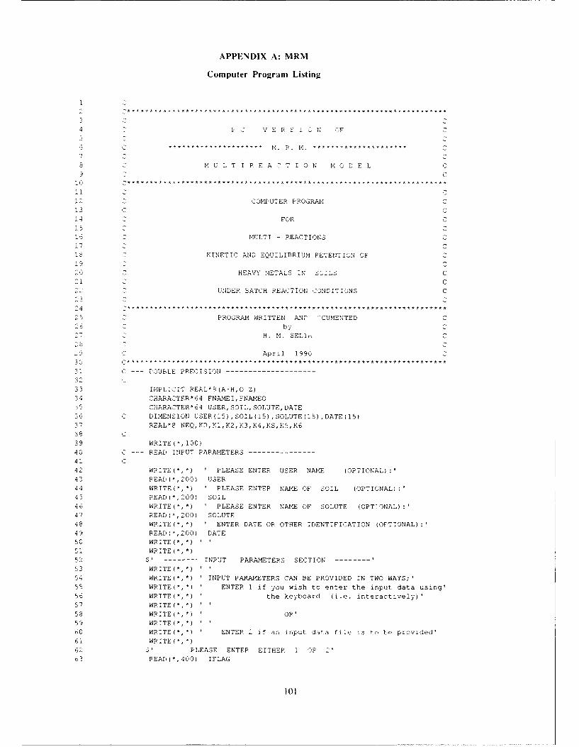
APPENDIX A: MRM

Computer Program Listing

1c2 *************************************************************

3 C C

4 P C V E R S I 0 N OF5 CC-S C6C******************************M. F.. M1. ****************** C

7 C CS C M U L T I R E A C T I O N MO D E L C

9 CC

10****************************************************************

11 c

12 COMPUTER PROGRAM C13 C14 FOR C15 C16 MULTI - REACTIONS C17 C1 C KINETIC AND EQUILIBRIUM RETENTION OF C19 , C20 C HEAVY METALS IN SOuLS C

1 CUNDER BATCH REACTION CONDITIONS C

C24 :********************************************************************

25 PROGRAM WRITTEN ANP 'CUMENTED Cby C

H. M. SEL1l, C

CApril 1990 C

30 * ***** ******.*********************************

31 C --- DOUBLE PRECISION---------------------32

33 IMPLICIT REAL*8(A-H,O-Z)34 CHARACTER*64 FNAMEI,FNAMEO

3S CHARACTER*64 USER, SOIL, SOLUTE, DATE36 C DIMENSION USER(15),SOIL(15),SOLUTE(15),DATE(15)

37 REAL*8 NEQ,KD, K1,K2, K3,K4,KS, K5, K638 C

39 WRITE(*,100)

40 C --- READ INPUT PARAMETERS----------------

41 C42 WRITE(*,*) ' PLEASE ENTER USER NAME (OPTIONAL):'43 READ (*, 200) USER44 WRITE(-,*) ' PLEASE ENTER NAM4E OF SOIL (OPTIONAL)

45 READ (*, 200) SOIL46 WRITE(*,*) PLEASE ENTER NAME OF SOLUTE (OPT-ONAL):'

47 READ(',200) SOLUTE48 WRITE(*,*) ' ENTER DATE OR OTHER IDENTIFICATION (OPTIONAL):'

49 READ(*,200) DATE5 WRITE(*,*)

51 WRITE(-,*)

52 $ ' ---- INPUT PARAMETERS SECTION53 WRITE(*,*)54 WRITE(*,*) INPUT PARAMAETERS CAN BE PROVIDED IN TWO WAYS;'

55 WRITE(*,*) ENTER 1 it you wish to enter the input data using'56 WRITE(*,*) the keyboard (i.e. interactively)'57 WRITE(*, *)58 WRITE(*, *) OR'59 WRITE(*,*)60 WRITE(*,*) ENTER 2 if an input data file is to be provided'

6i WRITE(t,-)

62 $' PLEASE ENTER EITHER 1 OR 2'

63 PEAD(*,400) IFLAG

I0I

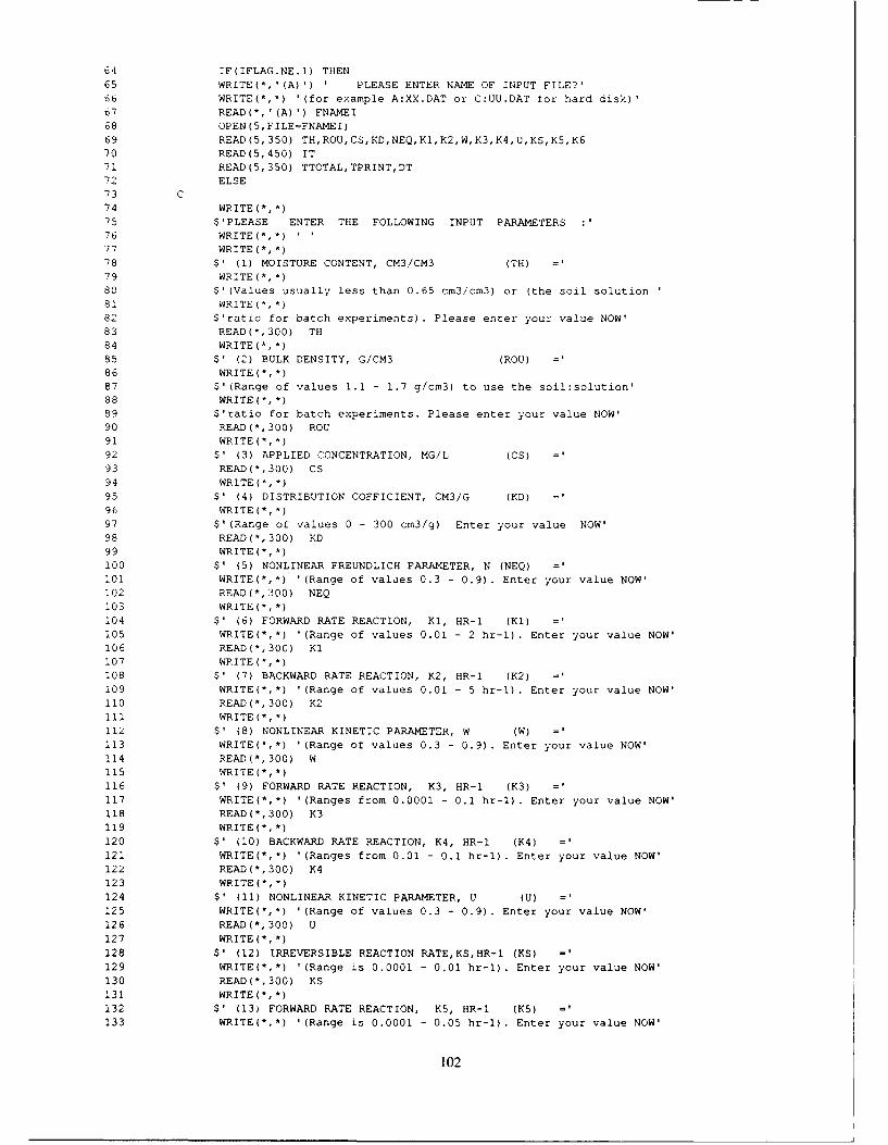
64 IF(IFLAG.NE.1) THEN

65 WRITE(*,'(A)') ' PLEASE ENTER NAME OF INPUT FILE?'

6b WRITE(*,*) '(for example A:XX.DAT or C:UU.DAT for hard disk)'

67 READ(*,'(A)') FNAMEI68 OPEN(5,FILE=FNAMEI)69 READ(5,350) TH,ROU,CS,KD,NEQ,K1,K2,W,K3,K4,U,KS,K5,K6

70 READ(5,450) IT71 READ(5,350) TTOTAL,TPRINT,DT

72 ELSE73 C

74 WRITE(*,*)

75 $'PLEASE ENTER THE FOLLOWING INPUT PARAMETERS

76 WRITE(,*)77 WRITE(*,*)

78 $' (1) MOISTURE CONTENT, CM3/CM3 (TH) =79 WRITE(*,*)80 $' (Values usually less than 0.65 cm3/cm3) or (the soil solution

81 WRITE(,*)82 $'ratio for batch experiments). Please enter your value NOW'

83 READ(*,300) TH84 WRITE(*,*)85 $' (2) BULK DENSITY, G/CM3 (ROU)

86 WRITE(*,*)87 $' (Range of values 1.1 - 1.7 g/cm3) to use the soil:solution'

88 WRITE(*,*)89 $'ratio for batch experiments. Please enter your value NOW'

90 READ(*,300) ROU91 WRITE(*,*)92 $' (3) APPLIED CONCENTRATION, MG/L (CS) ='

93 READ(*,300) CS

94 WRITE(*,*)95 $' (4) DISTRIBUTION COFFICIENT, CM3/G (KD) ='

96 WRITE(*,*)97 $'(Range of values 0 - 300 cm3/g) Enter your value NOW'

98 READ(*,300) KD99 WRITE(*,*)

100 $ (5) NONLINEAR FREUNDLICH PARAMETER, N (NEQ)101 WRITE(*,*) '(Range of values 0.3 - 0.9). Enter your value NOW'

102 READ(*,300) NEQ

103 WRITE(*,*)

104 $' (6) FORWARD RATE REACTION, Kl, HR-I (KI) ='105 WRITE(*,*) '(Range of values 0.01 - 2 hr-i). Enter your value NOW'106 READ(*,300) KI

107 WRITE(-,*)108 $' (7) BACKWARD RATE REACTION, K2, HR-I (K2) -'

109 WRITE(*,*) '(Range of values 0.01 - 5 hr-i). Enter your value NOW'

110 READ( ,300) K2

ill WRITE(*,*)112 $' (8) NONLINEAR KINETIC PARAMETER, W (W) ='113 WRITE(*,*) '(Range of values 0.3 - 0.9). Enter your value NOW'

114 READ(*,300) W

115 WRITE(*, *)116 $' (9) FORWARD RATE REACTION, K3, HR-I (K3)

117 WRITE(*,*) '(Ranges from 0.0001 - 0.1 hr-i). Enter your value NOW'

118 READ(*,300) K3119 WRITE(*,*)

120 $' (10) BACKWARD RATE REACTION, K4, HR-i (K4) ='121 WRITE(*,*) '(Ranges from 0.01 - 0.1 hr-i). Enter your value NOW'

122 READ(*,300) K4

123 WRITE(*,*)124 $' (11) NONLINEAR KINETIC PARAMETER, U (U) ='

125 WRITE(*,*) '(Range of values 0.3 - 0.9). Enter your value NOW'

126 READ(*,300) U

127 WRITE(*,*)128 $' (12) IRREVERSIBLE REACTION RATE,KS,HR-1 (KS) -,

129 WRITE(*,*) '(Range is 0.0001 - 0.01 hr-i). Enter your value NOW'

130 READ(*,300) KS

131 WRITE(*,*)132 $' (13) FORWARD RATE REACTION, K5, HR-i (K5)133 WRITE(*,*) '(Range is 0.0001 - 0.05 hr-i). Enter your value NOW'

102

134 READ(*,300) K5135 WRITE(*,*)

136 ' (14) BACKWARD RATE REACTION, K6, HR-I (K6)137 WRITE(*,*) '(Range is 0.001 - 0.1 hr-i). Enter your value NOW'138 READ(*,300) K6139 WRITE(*,*)

140 $' (15) NUMBER OF ITERATIONS (IT) AN INTEGER (FROM 0 TO 9)1141 READ(*,400) IT142 WRITE(*,*)

143 $' (16) TOTAL SIMULATION TIME, HOURS (TTOTAL) =144 READ(*,300) TTOTAL145 WRITE(*,*)146 $' (17) PRINTOUT TIME DESIRED, HOURS (TPRINT)147 READ(*,300) TPRINT148 WRITE(*,*)

149 $' (18) INCREMENTAL TIME STEP, HOURS (DT)150 WRITE(*,*)151 $. A default value of Dt=0.02 is given152 READ(*,300) DDT

153 ENDIF

154 C155 PIN=0.02

156 IF(DDT.NE.0.0) THEN157 DT=DDT158 ELSE

159 DT=PIN160 ENDIF

161 C162 WRITE(*,1(A)') ' PLEASE ENTER NAME OF OUTPUT FILE (FOR EXAMPLE163 * B:ZZ.DAT)'164 READ(*,'(A)') FNAMEO

165 OPEN(6,FILE=FNAMEO,STATUS='UNKNOWN')166 C --- WRITE TITLE HEADING

167 WRITE(6,100)

168 C169 C --- WRITE INPUT PARAMETERS

170 C171 WRITE(6,200) USER

172 WRITE(6,200) SOIL

173 WRITE(6,200) SOLUTE174 WRITE(6,200) DATE175 WRITE(6,500) TH,ROU,CS,KD,NEQ,K1,K2,W,K3,K4,U,KS

176 WRITE(6,600) K5,K6, IT,TTOTAL,TPRINT,DT

177 C

178 WRITE(*,*) '------- Execution Begins179 WRITE(*,*) 1 '180 C --- INITIAL CONDITIONS (TIME = 0)

181 C182 TIME=0.ODO

183 TI=DT

184 C=CS185 CX=0.ODO

186 SINPUT=TH*CS

187 SE=0.ODO

188 Sl=0.ODO

189 S2=0.ODO

190 S3=0.ODO

191 SEX=SE

192 S1X=S1193 $2X=$2

194 $3X=$3

195 SIR=0.ODO

196 C197 C --- CALCULATION OF OUTPUT TIME STEPS AND TOTAL OUTPUT

198 C199 II=TPRINT/TI+0.5DO

200 JJ=TTOTAL/TI+0.5DO

201 KK=JJ/II+0.5D0

202 C

203 C --- WRITE SIMULATION OUTPUT DATA COLUMN HEADINGS

103

204 C205 WRITE(6,700)206 WRITE(*,700)

207 C

208 C --- BEGIN SIMULATION209 C

210 C CALCULATION OF S-EQUILIBRIUM AT TIME ZERO

211 C

212 COE=C+(ROU/TH)*SE

213 CEX=C214 C

215 C --- ITERATION FOR S-EQUILIBRIUM CALCULATIONS

216 C217 IF(KD.EQ.0.ODO) GO TO 20218 IF(COE.LT.10.OE-20) GO TO 20

219 5 CONTINUE220 DO 10 IE=1,5

221 C=CEX

222 10 CEX=COE/(1+KD*(ROUTH)*C**(NEQ-1.0))

2 IF(DABS((CEX-C)).LT.1.OD-06) GO TO 15

224 GO TO 5

225 15 C=CEX

226 SE=KD*C**NEQ227 20 CONTINUE

228 C

229 C ----------- CALCULATIONS AT TIMES GREATER THAN ZERO

230 IT=IT+1231 DO 70 K=1,KK

232 DO 60 J=1,II233 DO 30 I=1, IT

234 C235 C --- EXPLICIT-IMPLICIT FINITE DIFFERENCE CALCULATIONS236 C

237 Xl=TI*(Kl*(((C+CX)/2)**W)-K2*(ROU/TH)*((S1+SIX)!2))

238 X2=TI*(K3*(((C+CX)/2)**U)-K4*(ROU/TH)*((S2+S2X)/2))

239 X3=TI*KS*((C+CX)/2)240 CX=C-(X1+X2+X3)

241 SlX=SI+XI*(TH/ROU)

242 S2X=S2+X2*(THROU)+TI*(K6*((S3+S3X)/2)-K5*((S2+S2X),i2))

243 S3X=S3+TI*(K5*((S2+S2X)/2)-K6*((S3+S3X)!2))

244 30 CONTINUE245 C=CX

246 S1=SIX

247 $2=$2X

248 $3=$3X249 SIR=SIR+TI*KS*(TH/ROU)*C

250 C

251 C252 C ------------ ITERATION FOR SE CALCULATIONS253 COE=C+(ROU/TH)*SE254 IF(COE.LT.10.OE-20) GO TO 50

255 CEX=C256 35 CONTINUE257 DO 40 IE=1,5

258 C=CEX

259 40 CEX=COE/(1+KD*(ROU/TH)*C**(NEQ-1.0DO))

260 IF(DABS((CEX-C)).LT.1.OD-06) GO TO 45261 GO TO 35

262 45 C=CEX

263 SE=KD*C**NEQ264 CX=C

265 50 CONTINUE

266 C

267 C268 60 CONTINUE269 C

270 C--- MASS BALANCE CALCULATIONS

271 C272 BAL=100*(C*TH+ROU*(SE+SI+S2+S3+SIR))/SINPUT273 TOTALS=SE+S+S2+S3+SIR

104

274 C

275 C --- WRITE OUTPUT DATA AT DESIRED SIMULATION TIMES---------

276 C

277 TIME=K*TPRINT

278 WRITE(6,800) TIME,C,SE,S1,S2,S3,SIR,TOTALS,BAL

279 WRITE(*,800) TIME,C,SE,SI,S2,S3,SIR,TOTALS,BAL

280 70 CONTINUE

281 C

282 C --- FORMAT STATEMENTS ---

283 C284 C

285 100 FORMAT(//,7X,

286 & **********************************************************287 $//,7X,

288 & WELCOME TO

289 $//,7X,

290 &1 P C V E R S I 0 N OF

291 $//,7X,

292 &1 M. R. M.

293 $//,7X,

294 & SIMULATION MODEL FOR KINETIC

295

296 & RETENTION OF HEAVY METALS IN SOILS

297 $//,7X,

298 & UNDER NO - FLOW CONDITIONS

299

300 $//,7X,

301 &***********************************************************302 $/,7X,

303 &. PROGRAM WRITTEN AND DOCUMENTED

304 $/,7X,

305 &' by

306 $/,7X,

307 &' H. M. SELIM

308 $/,7X,

309 &' April 1990

310 $/,7X,

311 *************

312313 200 FORMAT(A64)

314 300 FORMAT(F12.0)

315 350 FORMAT(50X,E20.6)

316 400 FORMAT(If)

317 450 FORMAT(50X,I3)

318 500 FORMAT(//,

319 $2X,'INPUT PARAMETERS :,//

320 $5X,'1. MOISTURE CONTENT, CM3/CM3 (TH) =',F10.5,/

321 $5X,'2. BULK DENSITY, G/CM3 (ROU) =',FIO.5,/

322 $5X,'3. APPLIED CONCENTRATION, MG/L (CS) =',F10.5,/

323 $5X,'4. DISTRIBUTION COEFFICIENT, KD,CM3/G (KD) =',F10.5,/

324 $5X,-5. NONLINEAR FREUNDLICH PARAMETER, N (NEQ) =',FIO.5,/

325 $5X,'6. FORWARD RATE REACTION, Kl,HR-1 (KI) =',FIO.5,/

326 $5X,'7. BACKWARD RATE REACTION, K2,HR-1 (K2) =',F0.5,/

327 $5X,'8. NONLINEAR KINETIC PARAMETER, W, (W) =',Fl0.5,/

328 $5X, '9. FORWARD RATE REACTION, K3,HR-1 IK3) =',FIO.5,/

329 $4X,'10. BACKWARD RATE REACTION, K4,HR-1 (K4) =',FIO.5,/

330 $4X,111. NONLINEAR KINETIC PARAMETER, U, (U) =',F1O.5,/

331 $4X,'12. IRREVERSIBLE REACTION RATE,KS,HR-1 (KS) =',F0.5)

332 600 FORMAT(

333 $4X, '13. FORWARD RATE REACTION, K5,HR-1 (K5) =',F10.5,/

334 $4X,'14. BACKWARD RATE REACTION, K6,HR-l (K6) =',F1O.5,/

335 $4X,'15. NUMBER OF ITERATIONS, M (IT) =',I10,/

336 $4X,'16. TOTAL SIMULATION TIME,HOURS (TTOTAL) =',FO.5,/

337 $4X, '17. PRINTOUT TIME DESIRED, HOURS (TPRINT) =',FI0.5,/

338 $4X,-18. INCREMENTAL TIME STEP,HOURS (DT) =',FI0.5,////)

339 700 FORMAT(////// ,72(lH*)//IH ,27X,'SIMULATION RESULTS'/

340 172(1H*)// ,lX,

341 *'TIME SOLUTION EQUIL KINETIC KINETIC KINETIC IRREV. TOTAL

342 * MASS'/,8X,'CONC.',3X,

343 *'PHASE PHASE 1 PHASE 2 PHASE 3 SINK SORBED BALANCE'/i/,

105

344 *'T C SE Sl S2 S3 SIR S345 * '/

346 4X,'--MG/L--',4X,

347 1 --------------------- MG/KG ----------------------- /)348 800 FORMAT(lX,F6.1,1X,FS.4,lX,F7.4,lX,F7.3,349 *3X,3(F8.3,lX),F7.3,lX,F7.2)

350 WRITE(*,*)351 WRITE(*,*) ------- Requested Simulations Completed ------

352 WRITE(*,*)353 WRITE(*,*) .------ MRM TERMINATED SUCCESSFULLY --------354 WRITE(*,*)355 WRITE(*,*) '----- THANK YOU FOR USING MRM ----------356 END

106

Sample of MRM Input Data

1. MOISTURE CONTENT, CM3/CM3 (TH) = 0.500EOO

2. BULK DENSITY, G/CM3 (ROU) = 1.250E003. APPLIED CONCENTRATION, MG/L (CS) = 10.OOOEOO4. DISTRIBUTION COEFFICIENT, KD, CM3/i (KD) = 1.OOOEOO

5. NONLINEAR FREUNDLICH PARAMETER, N (NEQ) = 0.500E006. FORWARD RATE REACTION, Ki, HR-i (KI) = 0.010E00

7. BACKWARD RATE REACTION, K2, HR-I (K2) = 0.100E00

8. NONLINEAR KINETIC PARAMETER, W (W) = 0.750E009. FORWARD RATE REACTION, K3, HR-I (K3) = u.100E00

10. BACKWARD RATE REACTION, K4, HR-I (K4) = 0.100E00

11 NONLINEAR KINETIC PARAMETER, U (U) = 0.900E0012. IRREVERSIBLE REACTION RATE, KS, HR-i (KS) = 0.001E00

13. FORWARD RATE REACTION, K5, HR-i (K5) = 0.010E00

14. BACKWARD RATE REACTION, K6, HR-i (K6) = 0.100E0015. NUMBER OF ITERATIONS, M (IT) = 00016. TOTAL SIMULATION TIME, HOURS (TTOTAL) = 50.000E00

17. PRINTOUT TIME DESIRED, HOURS (TPRINT) = 1.000E00

18. TIME STEP, HOURS (DT) = 0.100E00

107

MRM Computer Program Output Listing

WELCOME TO

P C VERSION OF

M. R. M.

SIMULATION MODEL FOR KINETIC

RETENTION OF HEAVY METALS IN SOILS

UNDER NO - FLOW CONDITIONS

* ** **** ** **** **** ** ********* ********* **** *************** ****

PROGRAM WRITTEN AND DOCUMENTED

by

H. M. SELIM

February 1990

INPUT PARAMETERS1. MOISTURE CONTENT,CM3/CM3 (TH) = .50000

2. BULK DENSITY,G/CM3 (ROU) = 1.25000

3. APPLIED CONCENTRATION, MG/L (CS) = 10.000004. DISTRIBUTION COEFFICIENT, KD, CM3/G (KD) = 1.00000

5. NONLINEAR FREUNDLICH PARAMETER, N (NEQ) = .50000

6. FORWARD RATE REACTION, KI,HR-1 (KI) = .010007. BACKWARD RATE REACTION, K2,HR-1 (K2) = .100008. NONLINEAR KINETIC PARAMETER, W, (W) = .75000

9. FORWARD RATE REACTION, K3, HR-i (K3) .10000

10. BACKWARD RATE REACTION, K4, HR-i (K4) = .10000

11. NONLINEAR KINETIC PARAMETER, U, (U) = .9000012. IRREVERSIBLE REACTION RATE,KS,HR-1 (KS) = .00100

13. FORWARD RATE REACTION, K5,HR-1 (K5) = .01000

14. BACKWARD RATE REACTION, K6,HR-1 (K6) = .1000015. NUMBER OF ITERATIONS, M (IT) = 0

16. TOTAL SIMULATION TIME,HOURS (TTOTAL) = 50.0000017. PRINTOUT TIME DESIRED,HOURS (TPRINT) = 1.0000018. INCREMENTAL TIME STEP,HOURS (DT) = .02000

108

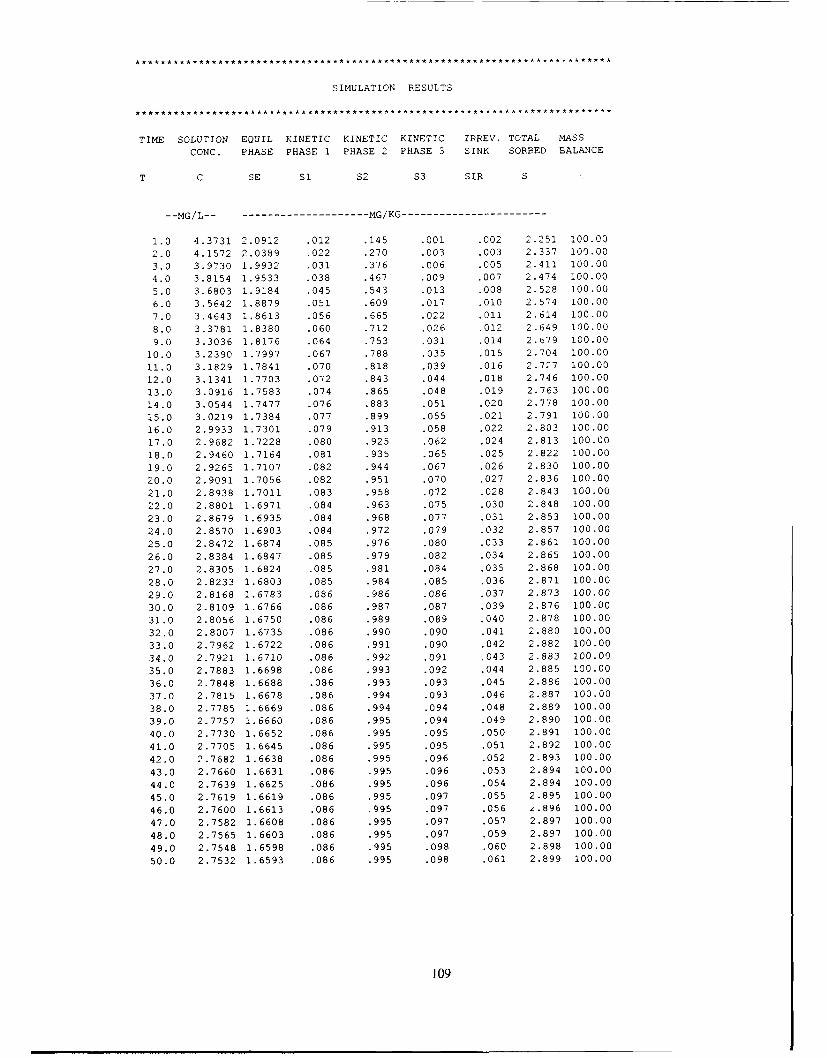
SIMULATION RESULTS

TIME SOLUTION EQUIL KINETIC KINETIC KINETIC IRREV. TOTAL MASS

CONC. PHASE PHASE 1 PHASE 2 PHASE 3 SINK SORBED BALANCE

T C SE S1 S2 S3 SIR S -

--MG/L-- -------------------- MG/KG------------------------

1.0 4.3731 2.0912 .012 .145 .001 .002 2.251 100.00

2.0 4.1572 2.0389 .022 .270 .003 .003 2.337 100.00

3.0 3.9730 1.9932 .031 .376 .006 .005 2.411 100.00

4.0 3.8154 1.9533 .038 .467 .009 .007 2.474 100.00

5.0 3.6803 1.9184 .045 .543 .013 .008 2.528 100.00

6.0 3.5642 1.8879 .051 .609 .017 .010 2.574 100.00

7.0 3.4643 1.8613 .056 .665 .022 .011 2.614 100.00

8.0 3.3781 1.8380 .060 .712 .026 .012 2.649 100.00

9.0 3.3036 1.8176 .064 .753 .031 .014 2.679 100.00

10.0 3.2390 1.7997 .067 .788 .035 .015 2.704 100.00

11.0 3.1829 1.7841 .070 .818 .039 .016 2.727 100.00

12.0 3.1341 1.7703 .072 .843 .044 .018 2.746 100.00

13.0 3.0916 1.7583 .074 .865 .048 .019 2.763 100.00

14.0 3.0544 1.7477 .076 .883 .051 .020 2.778 100.00

15.0 3.0219 1.7384 .077 .899 .055 .021 2.791 100.00

16.0 2.9933 1.7301 .079 .913 .058 .022 2.803 100.00

17.0 2.9682 1.7228 .080 .925 .062 .024 2.813 100.00

18.0 2.9460 1.7164 .081 .935 .065 .025 2.822 100.00

19.0 2.9265 1.7107 .082 .944 .067 .026 2.830 100.00

20.0 2.9091 1.7056 .082 .951 .070 .027 2.836 100.00

21.0 2.8938 1.7011 .083 .958 .072 .028 2.843 100.00

22.0 2.8801 1.6971 .084 .963 .075 .030 2.848 100.00

23.0 2.8679 1.6935 .084 .968 .077 .031 2.853 100.00

24.0 2.8570 1.6903 .084 .972 .079 .032 2.857 100.00

25.0 2.8472 1.6874 .085 .976 .080 .033 2.861 100.00

26.0 2.8384 1.6847 .085 .979 .082 .034 2.865 100.00

27.0 2.8305 1.6824 .085 .981 .084 .035 2.868 100.00

28.0 2.8233 1.6803 .085 .984 .085 .036 2.871 100.00

29.0 2.8168 1.6783 .086 .986 .086 .037 2.873 100.00

30.0 2.8109 1.6766 .086 .987 .087 .039 2.876 100.00

31.0 2.8056 1.6750 .086 .989 .089 .040 2.878 100.00

32.0 2.8007 1.6735 .086 .990 .090 .041 2.880 100.00

33.0 2.7962 1.6722 .086 .991 .090 .042 2.882 100.00

34.0 2.7921 1.6710 .086 .992 .091 .043 2.883 100.00

35.0 2.7883 1.6698 .086 .993 .092 .044 2.885 100.00

36.0 2.7848 1.6688 .086 .993 .093 .045 2.886 100.00

37.0 2.7815 1.6678 .086 .994 .093 .046 2.887 100.00

38.0 2.7785 1.6669 .086 .994 .094 .048 2.889 100.00

39.0 2.7757 1.6660 .086 .995 .094 .049 2.890 100.00

40.0 2.7730 1.6652 .086 .995 .095 .050 2.891 100.00

41.0 2.7705 1.6645 .086 .995 .095 .051 2.892 100.00

42.0 2.7682 1.6638 .086 .995 .096 .052 2.893 100.00

43.0 2.7660 1.6631 .086 .995 .096 .053 2.894 100.00

44.0 2.7639 1.6625 .086 .995 .096 .054 2.894 100.00

45.0 2.7619 1.6619 .086 .995 .097 .055 2.895 100.00

46.0 2.7600 1.6613 .086 .995 .097 .056 2.896 100.00

47.0 2.7582 1.6608 .086 .995 .097 .057 2.897 100.00

48.0 2.7565 1.6603 .086 .995 .097 .059 2.897 100.00

49.0 2.7548 1.6598 .086 .995 .098 .060 2.898 100.00

50.0 2.7532 1.6593 .086 .995 .098 .061 2.899 100.00

109

APPENDIX B: MRTM

Computer Program Listing

1 C

3 C C4 C M. R. T. M. C5 C C6 * ** ******************* *************

7 C C8 C COMPUTER PROGRAM C9 C C

10 C FOR THE SIMULTANEOUS TRANSPORT AND RETENTION C11 C OF HEAVY METALS C12 C IN THE SOIL PROFILE C13 C USING C14 C THE SOLUTE CONVECTION - DISPERSION EQUATION C15 C AND C16 C MULTIREACTION MECHANISMS C17 C OF C18 C NONLINEAR EQUILIBRIUM AND KINETIC REACTIONS C19 C C20 C C21 ***** ****tttt *********tt***********t** ********22 C PROGRAM WRITTEN AND DOCUMENTED C23 C H. M. SELIM C24 C by C25 C 1990 C2627 C C28 IMPLICIT REAL*8(A-H,O-Z)29 CHARACTER*64 FNAMEI,FNAMEO30 COMMON/Li/ C(101),DC(101),DU(101),DL(101),E(101),S1(101),S2(101)31 COMMON/L2/ SIR(101),CX(101),S1X(101),S2X(101)32 COMMON/L3/ X(101),S3(101),S3X(101)33 COMMON/L4/ TH,ROU,COL,WFLX,CI,CS, D,K1,K2,W,K3,K4,U,KS,K5,K6,KD34 COMMON/L5/ NEQ,IT,N,NM1,NP135 COMMON/L6/ TPULSE,TTOTAL, TPRINT,DT,DX, GAMMA, BETA36 CHARACTER-64 USER, SOIL, SOLUTE,DATE37 REAL*8 KI,K2,K3,K4,K5,K6,KS,KD,NEQ

38 C39 C40 WRITE(*,100)41 C --- READ INPUT PARAMETERS----------------42 C43 WRITE(*,*) PLEASE ENTER USER NAME (OPTIONAL):'44 READ(*,800) USER45 WRITE(*,*) ' PLEASE ENTER NAME OF SOIL (OPTIONAL):'46 READ(*,800) SOIL47 WRITE(*,*) ' PLEASE ENTER NAME OF SOLUTE (OPTIONAL):'48 READ(*,800) SOLUTE49 WRITE(*,*) ' ENTER DATE OR OTHER IDENTIFICATION (OPTIONAL):'50 READ(*,800) DATE51 WRITE(*,*) '52 WRITE(*,*)53 $' - -------- INPUT PARAMETERS SECTION -54 WRITE(*,*) '55 WRITE(*,*) INPUT PARAMETERS CAN BE PROVIDED IN TWO WAYS;'56 WRITE(*,*) ENTER 1 if you wish to enter the input data using'57 WRITE(*,*) the keyboard (i.e. interactively)'58 WRITE(*,*) '59 WRITE(*,*) OR'60 WRITE(*,*) '61 WRITE(*,*) ENTER 2 if an input data file is to be provided'62 WRITE(*,*)63 $' PLEASE ENTER EITHER 1 OR 2'64 READ(*,950) IFLAG65 IF(IFLAG.NE.1) THEN66 WRITE(*,'(A)') ' PLEASE ENTER NAME OF INPUT FILE?'67 WRITE(*,*) '(for example A:XX.DAT or C:UU.DAT for hard disk)'68 READ(*,'(A)') FNAMEI69 OPEN(5,FILE=FNAMEI)70 C

III

71 C72 READ(5,700) TH,ROU,COL,WFLX73 READ(5,700) CI,CS,D74 READ(5,700) KD,NEQ

75 READ(5,700) K1,K2,W76 READ(5,700) K3,K4,U77 READ(5,700) KS78 READ(5,700) K5,K679 READ(5,750) IT80 READ(5,700) TPULSE,TTOTAL,TPRINT,DT,DX81 ELSE82 C

83 WRITE(*,*)84 $'PLEASE ENTER THE FOLLOWING INPUT PARAMETERS85 WRITE(*,*)86 WRITE(*,*)87 $' (1) MOISTURE CONTENT, CM3/CM3 (TH)88 WRITE(*,*)89 $' (Values usually less than 0.65 cm3/cm3) . Enter your value NOW'90 READ(*,900) TH91 WRITE(*,*)92 $' (2) BULK DENSITY, G/CM3 (ROU)93 WRITE(*,*)94 $' (Range of values 1.1 - 1.7 g/cm3) . Ent-r your valuc !:OW'95 READ(*,900) ROU96 WRITE(*,*)97 $' (3) PROFILE OR SOIL COLUMN LENGTH, CM (COL)98 READ(*,900) COL99 WRITE(*,*)100 $' (4) WATER FLUX, CM/-OUR (WFLX)101 WRITE(*,*)102 $'(Range of values 0.01 - 5 cm/hr). Enter your value NOW'103 READ(*,900) WFLX104 WRITE(*,*)105 $' (5) INITIAL CONCENTRATION, MG!L (CI)106 READ(*,900) CI107 WRITE(*,*)108 $' (6) APPLIED CONCENTRATION, MG/L (CS)109 READ(*,900) CS110 WRITE(*,*)111 $' (7) DISPERSION COEFFICIENT,D, CM2/HOUR (D)112 WRITE(*,*)113 $'(Range of values 0.1 - 1.5 cm2/hour). Enter your value NOW'114 READ(*,900) D115 WRITE(*,*)116 $' (8) DISTRIBUTION COEFFICIENT, KD (KD)117 WRITE(*,*)118 $' (Range of values 0 - 300 cm3/g) Enter your value NOW'119 READ(*,900) KD120 WRITE(*,*)121 ' (9) NONLINEAR FREUNDLICH PARAMETER, N (NEQ)122 WRITE(*,*) '(Range of values 0.3 - 0.9). Enter your value NOW'123 READ(*,900) NEQ124 WRITE(*,*)125 $' (10) FORWARD RATE REACTION, KI, HR-i (KI)126 WRITE(*,*) '(Range of values 0.01 - 2 hr-i). Enter your value NOW'127 READ(*,900) KI128 WRITE(*,*)129 $' (11) BACKWARD RATE REACTION, K2, HR-i (K2)130 WRITE(*,*) '(Range of values 0.01 - 5 hr-i). Enter your value NOW'131 READ(*,900) K2132 WRITE(*,*)133 $' (12) NONLINEAR KINETIC PARAMETER, W, (W)134 WRITE(*,*) '(Range of values 0.3 - 0.9). Enter your value NOW'135 READ(*,900) W136 WRITE(*,*)137 $' (13) FORWARD RATE REACTION, K3, HR-I (K3)138 WRITE(*,*) '(Ranges from 0.0001 - 0.1 hr-i). Enter your value NOW'139 READ(*,900) K3140 WRITE(*,*)141 $' (14) BACKWARD RATE REACTION, K4, HR-i (K4)142 READ(*,900) K4143 WRITE(*,*) '(Ranges from 0.01 - 0.1 hr-1). Enter your value NOW'144 WRITE(*,*)145 $' (15) NONLINEAR KINETIC PARAMETER, U, (U)146 WRITE(*,*) '(Range of values 0.3 - 0.9). Enter your value NOW'

112

147 READ (-, 900) U148 WRITE(',-)149 $ (16) IRREVERSIBLE REAJTION PATE,KS,HR-1 (KS)150 WRITE(*,*) '(Range is 0.0001 - 0.01 hr-i). Enter your value NOW'151 READ)(, 900) KS152 WRITE(*,*)153 $' (17) FORWARD RATE REACTION, K5,H R-i (KS)154 WRITE(*, *) '(Range is 0.0001 - 0.01 hr-I). Enter your value NOW'155 READ(*,900) K5156 WRITE(*,*)157 $' (18) BACKWARD RATE REACTION, K6, HR-i (P-6)158 WRITE(*,*) '(Range is 0.001 - 0.1 hr-i). Enter your value NOW'159 READ(*,900) K6160 WRITE(,*)161 $' (19) NUMBER OF ITERATIONS (IT) AN INTEGER (FROM 0 TO 9)162 READ(*,950) IT163 WRITE(*,*)164 $' (20) INPUT PULSE DURATION, HOURS (TPULSE)165 READ(*,900) TPULSE166 WRITE(*,*)167 $' (21) TOTAL SIMULATION TIME, HOURS (TTOTAL)168 READ(*,900) TTOTAL169 WRITE(*,-)170 $' (22) PRINTOUT TIME DESIRED, HOURS (TPRINT)171 READ(*, 900) TPRINT172 WRITE)*,*)173 $' (23) INCREMENTAL TIME STEP, HOURS (DT)174 WRITE(*,*)175 $. A default value of DT=0.02 is given176 READ(*,900) DDT177 WRITE(*,*)178 $' (24) INCREMENTAL DEPTH, CM (DX)179 WRITE(*,*)180 S A default value of DX=1.00 is given181 READ(*,900) DDX182 ENDIF183184 XIN=1.00185 IF(DDX.NE.0.0) THEN

186 DX=DDX187 ELSE188 DX=XIN189 ENDIF190 C

191 PIN=0.02192 IF(DDT.NE.0.0) THEN193 DT=DDT194 ELSE195 DT=PIN196 ENDIF197 WRITE(*, ' (A)') PLEASE ENTER NAME OF OUTPUT FILE (FOR EXAMPLE198 ' B:ZZ.DAT)'199 READ(*, ' (A) ') FNAMEO200 OPEN (6, FI LE=FNAMEO, STATUS=' UNKNOWN'201 PV=WFLX/TH202 RS=N'EQ*ROU*KD,/TH203 Co=CS204 C205 TIME=0.ODO206 EF=0.ODO207 5 CONTINUE208 GAMMA=DT/ (2 .DO*DX*DX)209 BETA=DT!DX210 IF((BETA*PV).GT.0.50D0) GO TO 7211 IF((GA!IMA*CD/(BETA*PV)).LT.0.5D0) GO TO 6212 GO TO 8213 6 DX=DX/2214 GO TO 5215 7 DT=DT/2216 GO TO 5217 8 CONTINUE218 N=COL/DX

219 NM 1 =N- 1220 NM2=N-2221 NP1=N+1222 GAMMA=DT/(2*DX*DX)

113

223 BETA=DT!DX224 C225 IF(N.LT.500) GO TO 9226 WRITE(*,*) ' W A R N I N G227 WRITE(*,*)228 &'Dimension of variables exceeds 500. Did you increase array

sizes'229 WRITE(*,*)230 &' If not, the program will terminate abruptly (see text).'231 9 CONTINUE232

233 C--- WRITE TITLE HEADING234 WRITE(6,100)

235 WRITE(6,800) USER236 WRITE(6,800) SOIL237 WRITE( ,800) SOLUTE238 WRITE(6,800) DATE239 WRITE(6,300) TH,ROU,COL,WFLX,CI,CS,D,K1,K2,B,K3,K4,W,KS240 WRITE(6,310) K5,K6, IT,KD,NEQ241 &,TPULSE,TTOTAL, TPRINT242 WRITE(6,400) DX,DT243 C244 DO 10 I=I,NP1245 SI(I)=0.ODO246 S2(I)=0.ODO247 S3(I)=0.0D0248 SIR(I)=0.ODO249 SlX(I)=0.ODO250 S2X(I)=0.ODO251 S3X(I)=0.0DCl252 CX(I)=CI253 10 C(I)=CI254 WRITE(*,*) '------ INITIAL CONDITIONS COMPLETED --------255 C256 WRITE (*,*) --------- Execution Begins --------257 WRITE (*,*) ----------- Please Wait ------------258 IT=IT+l259 FF=2*DX260 NKK=TPRINT/DT+0.50DO261 KLM=TTOTAL/DTO'r-G 0262 KK=KLM/NFK< .5D0263 C264 L=0265 SINT=TiULSE*C7 , 1,X266 DO 50 JJ=1,KK267 DO 20 LL=1,NKK268 TT=LL*DT+(JJ-)*TPRINT269 IF(DABS(TT-TPULSE).LT.0.01D0) CS=0.ODO270 L=L+I271 CALL SMRTM272 EF=C(N)+EF273 20 CONTINUE

274 TIME=JJ*TPRINT275 C276 WRITE(6,500) TIME277 VV0=WFLX*TIME/(COL*TH)278 CC0=C(N)/C0279 WRITE(6,525) VVO,CC)280 WRITE(*,650) TIME,VVO,CCO281 WRITE(*,*) --------. Execution Continues -------

282 WRITE(*,*) --------- Please Wait ------------283 WRITE(6,550)284 DO 30 I=1,NP1285 DEPTH=DX*(I-1)286 SEQ=KD*C(I)**NEQ287 TOTAL=SEQ+SI(I)+S2(I)+S3(I)+SIR(I)288 30 WRITE(6,600) DEP-H,C(I),SEQ,S(I),S2(I),S3(I),SIR(I),TOTAL289 CALL INTEG(DX,C,.,NPI)290 TSWATR=TH*X(NPI)291 C292 DO 40 I=1,NPI293 40 E(I)=C(I)**NEQ294 CALL INTEG(DX,E,X,NP1)295 TSEQ=ROU*KD*X(NPl)296 SINP=TIME*CS*WFLX297 IF(SINP.GT.SINT) SINP=SINT

114

298 IF(CS.EQ.0.DO) SINP=SINT299300 CALL INTEG(DX,S1,X,NP1)301 TSKIN!=ROU*X(NPI)302303 CALL INTEG(DX,S2,X,NPI)304 TSKIN2=ROU'X(NPi)305 C306 CALL INTEG(DX,S3,X,NPI)j0

7 TSKIN3=ROU*X(NPI)

308 C309 TEFFL=DT*WFLX EF310 C311 CALL INTEG(DX,SIR,X,NP)312 TSIR=ROU*X(NPI)313 BAL=(TEFFL+TSKIN1+TSKIN2+TSKIN3+TSIR+TSEQ+TSWATR)*100.ODO/SINP314 WRITE(6,200)SINP,TSWATRTSEQ,TSKIN1,TSKIN2,TSKIN3,TSIRITEFFL,BAL315 50 CONTINUE316 C

317 ]20 FORMAT(//,7X,318

& **I **********************************************

319 $//,7X,320 &' M. R. T. M.

321322 & **********************************************

3 23323 $//,,7X,

324 &' SIMULATION RESULTS USING MRTM MODEL FOR TRANSPORT

325 $//,7X,326 &' AND

327 $//,7X,328 &' RETENTION 00 HEAVY METALS IN THE SOIL

329 $//,7x,330 &' UNDER

331 $//,7X,332 & STEADY WATER FLOW CONDITIONS

333 $/,,7X,334 $//,7X,335

&***********I*********** **** ***********************

336337 &' PROGRAM WRITTEN AND DOCUMENTED

338 $/,7X,339 V by

340341 &' H. M. SELIM

342 $/,7X,343 &' April 1990

344 $/,7X ,345

& I ************************************** **

*1)

346 200 FOR4AT(//,2X, 'S A L T B A L A N C E :',//347 &7X, 'TOTAL INPUT SOLUTE FROM PULSE (MG) =',F10.4,/348 &7X, 'TOTAL SOLUTE SOIL SOLUTION PHASE (MG) =',FI0.4,!,349 &7X, 'TOTAL SORBED IN (EQUILIB) PHASE SE (MG) ',FlO.4,/,

350 &7X, 'TOTAL SORBED IN (KINETIC) PHASE S1 (MG) =',FI0.4,!,351 &7X,'TOTAL SORBED IN (KINETIC) PHASE S2 (MG) ',F10.4,!,352 &7X,'TOTAL SORBED IN (KINETIC) PHASE S3 (MG) ',F10.4,/,

353 &7X,'TOTAL SORBED IN IRREVERSIBLE PHASE (MG) =' FI.4,/,354 &7X, 'TCTAL SOLUTE IN THE EFFLUENT (MG) ' FI0.4,/,355 &7X,'MASS BALANCE (CALC.OUTPUT/INPUT) U) ' F10.4,i)

356 300 FORMAT(//,357 $2X,'INPUT PARAMETEPS :',//

115

358 $5X, '1. MOISTURE CONTENT,CM3/CM3 (TH) =',FI0.5,/359 $5X, '2. BULK DENSITY,G/CM3 (ROU) =',F10.5,/360 $5X, '3. COLUMN LENGTH,CM (COL) =',FlO.5,/

361 $5X, '4. WATER FLUX,CM/HOUR (WFLX) =',FlO.5,/362 $5X, '5. INITIAL CONCENTRATION,MG/L (CI) =',FIO.5,/363 $5X,'6. CONCEN.IN INPUT PULSE,MG/L (CS) =',FlO.5,/364 $5X, 7. DISPERSION COEFFICIENT,CM2/HR (D) =',FIO.5,/365 $5X,'8. FORWARD RATE REACTION, KI,HR-1 (KI) =',FI0.5,/366 $5X, '9. BACKWARD RATE REACTION, K2,HR-1 (K2) =',F10.5,/367 $4X, '10. NONLINEAR KINETIC PARAMETER, W, (W) =',FI0.5,/368 $4X,'11. FORWARD RATE REACTION, K3,HR-1 (K3) =',F10.5,/369 $4X,'12. BACKWARD RATE REACTION, K4,HR-1 (K4) =',FIO.5,/370 $4X,'13. NONLINEAR KINETIC PARAMETER, U, (U) =',FIO.5,/

371 $4X,'14. IRREVERSIBLE REACTION RATE,KS,HR-1 (KS) =',FIO.5)372 310 FORMAT(373 $4X,'15. FORWARD RATE REACTION, K5,HR-1 (K5) =',FlO.5,/374 $4X,'16. BACKWARD RATE REACTION, K6,HR-1 (K6) =',FlO.5,/375 $4X, '17. NUMBER OF ITERATIONS (IT) =-,I10,/

376 $4X, '18. DISTRIBUTION COEFFICIENT FOR EQUILIBRIUM',/377 $4X,' SORPTION, KD, CM3/G (KD) =',F10.5,/378 $4X, '19. NONLINEAR PARAMETER FOR EQUILIBRIUM',/379 $4X, MECHANISM, NEQ (NEQ) =',F1O.5,/380 $4X, 20. INPUT PULSE DURATION,HR (TPULSE) =',F1O.5,/381 $4X, '21. TOTAL SIMULATION TIME, HR (TTOTAL) =',FIO.5,/382 $4X, '22. PRINTOUT TIME DESIRED,HR (TPRINT)

=',FI0.5,!/i/)

383 400 FORMAT(2X,'THE INCREMENTS USED WERE384 $5X, 'i. SIMULATION DEPTH INTERVAL,CM (DX) =',F10.5,/385 $5X,'2. INCREMENTAL TIME STEP,HR (DT) =',FlO.5,///)

386 500 FORMAT(/////////,387 $2X'S I M U L A T I 0 N T I M E (HOUR) =',F8.2/)388 525 FORMAT(389 $2X'PORE VOLUMES (V/V0) =',F10.2,X. 'REL. CONCENTRATION (C/CC)

390 &F8.4)391 550 FORMAT(///IH ,72(lH*)//lH ,20X,'CONCENTRATION DISTRIBUTION',392 *//ilH ,393 172(1H*)//IH ,2X,394 *'DEPTH SOLUT EQUIL KINETIC KINETIC KINETIC IRREV.395 * TOTAL'/,9X,'CONC.',4X,

396 *'PHASE PHASE 1 PHASE 2 PHASE 3 SINK SORBED'/,397 *' X C SE S1 S2 S3 SIR398 * S'//,IX399 1,' CM ',2X, '--MG/L--',2X,400 1' -------------------------MG/KG --------------------------

401 600 FORMAT(1X,F6.2,1X,F9.4,1X,F8.4,1X,F8.3,402 *1X, 3(F9.3,lX),F7.3)403 650 FORMAT(/////,2X,'SIMULATIONS ARE NOW COMPLETE UP TO',///,5X,

404 $'S I M U L A T I O N T I M E (HOUR) =',F8.2,//2X,405 $'PORE VOLUMES (V/V0) =',FI0.2,8X,'REL. CONCENTRATION (C/CC) =,

406 &F8.4//)407 700 FOPMAT(50X,E10.6)

408 750 FORMAT(50X,I3)409 800 FORMAT(A64)410 900 FORMAT(F12.0)411 950 FORMAT(If)412 WRITE(*,*)413 WRITE(*,*) ------- Requested Simulations Completed ----

414 WRITE(*,*)415 WRITE(*,*) '------- MRTM TERMINATED SUCCESSFULLY --------416 WRITE(*,*)417 WRITE(*,*) '---- THANK YOU FOR USING MRTM -----------418 END

419 C420 C421 C ***************************************************************422 C SUBROUTINE TRIDM GIVES A SOLUTION OF THE FINITE DIFFERENCE EQ.423 C OF THE CONVECTION-DISPERSION AND MULTIREACTION SYSTEM424 C425 C426 SUBROUTINE SMRTM427 IMPLICIT REAL*8(A-H,O-Z)428 COMMON/L1/ C(101),DC(101),DU(101),DL(101),E(101),Sl(101),S2(101)

429 COMMON/L2/ SIR(101),CX(101),SIX(101),S2X(101)430 COMMON/L3/ X(101),S3(101),S3X(101)431 COMMON/L4/ TH,ROU,COL,WFLX,CI,CS,D,K1,K2,W,K3,K4,U,KS,K5,K6,KD432 COMMON/L5/ NEQ, ITN,NMI,NP1

116

433 COMMON/L6/ TPULSE,TTOTAL..TPRINT,DT,DX,GAMMA,BETA434 REAL*S Kl,K2,K3,K4,K5,K6,KS, KD,NEQ435 C436 C437 FF=2*DX438 PV=WFLX/TH439 RS=NEQ*ROU*KD/TH440 C(1)=(WFLX*FF*CS+D*TH*C(3)l/(WFLX*FF+D*TH)441 DO 35 IJ=1,IT442 M=2443 DO 10 I=1,NMl444 DC(I)=l.0D0+2'.D0*GAMMA*D-BETA*PV445 DU (I) =BETA*PV-GAMMA*D446 E(I)=C(M)+GAMMA*D*(C(M+1)-42.ODO*C(M)+C(M-1))447 DL(I)=-GAM4A*D448 M=I+2449 10 CONTINUE450 M=N451 DC(NM1)=l.DO+GAMtMA*D452 E(1)=E(1)+GAMMA*D*C(l)453 C454 C INCORPORATION OF NONLINEAR KINETIC AND EQUILIBRIUM PROCESSES455 C (REVERSIBLE) IN MAIN DIAGONAL ELEMENTS AND RNS VECTOR456 C457 DO 20 I=1,NM1458 DC(I)=DC(I)+DT*KS/2459 R=0.ODO460 Hl=0.0D0461 H2=C.ODO462 IF((C(I±1).LT.1.OD-4).OR.(CX(I+1).LE.1.0D-4)) GO TO 15463 R=RS*(0.50D0*(C(I+1)+CX(I+1)))*,(NEQ-1.0D0)464 H1=(0.50D0*(C(I+1)+CX(I+1) ))**W4465 H2=(0.50D0*(C(I+1)+CX(I+l) ))**U466 15 DC(I)=DC(I)-4R467 E(I)=E(I)-DT*(Kl*Hl-K2*(ROU/TH)*(Sl1(+1)+Slx(I.1))/2)468 &-DT*(K3*H2-K4*(ROU/TH)*(S2(1+1)+S2X(I+1))/2)469 2 0 E (I) =E (I) +C (I+1) *R-DT* (KS/2) *((C (I+1) +CX (1+1)) /2)470 C471 CALL TRIDM(DC,DU,.DL,E,NM1)4'72 DO 25 I=2,N473 25 CX (I) =E (I -1)474 CX(NP1)=CX(N)475, CX(1)=C(1)4 7 DO 30 I=1,NP14'77 Hl=0.0D0478 H2=0.0D0479 IF(C(I).GT.1.OD-4) H1=((C(I)+CX(I))/2)**W480 IF(C(I).GT.1.OD-4) H2=((C(I)+CX(I))/2)**U481 S1X(I)=Sl(I)+DT*(K1*(TH/ROU)*Hl-K2*(S1(I)+S1X(I)(/2')482 S2x(I)=S2(I)+DT*K3*(TH/ROU)*H2-(K4+K5)*DT*(S2(I)+S2X(I))/2483 $+DT*K6*S3(I)484 30 CONTINUE485 35 CONTINUE486 C487 C488 DO 50 I=1,NP1489 C(I)=CX(I)490 S1(I)=S1X(I)491 S2(1)=S2X(I)

492 S3(I)=S3(I)+DT*K5S2 (I)493 $-DT*K6*S3(I)494 50 SIR(I)=SIR(I)+DT*KS*(TN/ROU)*C(I)495 RETURN496 END4QC7 C498 C ** * * *

499 C SUbR,:UTllE TRIDM GIVES A SOLUTION OF A TRIDIAGONAL MATRIX-VECTOR500 C EQUATION USING THOMAS ALGORITHM

501 C ***** * * " *

502 C503 SUBROUTINE TRIDM(A,B,C,D,N)504 IMPLICIT REAL*8(A-H,O-Z)505 DIMENSION A(N),B(N),C(N),D(N)506 DO 1 I=2,N507 C(I)=C(I) /A(I-1)

117

509 1 CONTINUE510 DO 2 I=2,N511 D(I)=D(I)-(C(I)*D(I-1))512 2 CONTINUE

513 D(N)=D(N)/A(N)514 DO 3 I=2,N515 D(N+I-I)=(D(N+I-I)-(B(N+I-I)*D(N+2-I)))/A(N+I-I)516 3 CONTINUE517 RETURN518 END519 C

520 C ************* ************* * *************521 C SUBROUTINE INTEG PERFORMS INTEGRATION OF A TABULAR FUNCTION Y522 C GIVEN AT EQUAL DISTANCES H USING TRAPEZOIDAL RULE.523 C ***************************************************************524 C525 SUBROUTINE INTEG(H,Y,Z,N)526 IMPLICIT REAL*8(A-H,O-Z)527 DIMENSION Y(N),Z(N)528 S2=0.0D0529 IF(N-1) 40,30,10530 10 HN=H/2.ODO531 DO 20 I =2,N532 S1=S2533 S2=S2+HH*(Y(I)+Y(I-1))534 20 Z(I-I)=S1

535 30 Z(N)=S2536 40 RETURN537 END

Sample of MRTM Input Data

1. MOISTURE CONTENT,CM3/CM3 (TH) = 0.400E002. BULK DENSITY,G/CM3 (ROU) = 1.250E003. COLUMN LENGTH,CM (COL) = 10.OOOEOO4. WATER FLUX,CM/HR (WFLX) = 1.OOOEOO5. INITIAL CONCENTRATION,MG/L (CI) = 0.OOOEOO6. CONCEN.IN INPUT PULSE,MG/L (CS) = 10.OOOEOO7. DISPERSION COEFFICIENT,D,CM2/HR (D) = 1.OOOEOO8. DISTRIB. COEFF. FOR EQL. SORP,CM3/G (KD) = 1.OOOEOO9. NONLINEAR PARAM.FOR EQUL. MECH. (NEQ) = 1.OOOEOO

10. FORWARD RATE REACTION, K1,HR-1 (KI) = 0.100EOO11. BACKWARD RATE REACTION, K2,HR-1 (K2) = 0.100EOO12. NONLINEAR KINETIC PARAMETER, W, (W) = 0.500E0013. FORWARD RATE REACTION, K3,HR-1 (K3) = 0.OOOEOO14. BACKWARD RATE REACTION, K4,HR-1 (K4) = 0.OOOEOO15. NONLINEAR KINETIC PARAMETER, U, (U) = 0.OOOEOO16. IRREVERSIBLE REACTION RATE,KS,HR-1 (KS) = 0.OOOEOO17. FORWARD RATE REACTION, K5,HR-1 (K5) = 0.OOOEOO18. BACKWARD RATE REACTION, K6,HR-1 (K6) = 0.OOOEOO19. NUMBER OF ITERATIONS (M) (IT) = 00020. INPUT PULSE DURATION,HR (TPULSE) = 12.000E0021. TOTAL SIMULATION TIME,HR (TTOTAL) = 16.000E0022. PRINTOUT TIME DESIRED,HR (TPRINT) = 4.000E0023. INCREMENTAL TIME STEP,HR (DT) = 0.200E0024. INCREMENTAL DEPTH, CM (cX) = 1.OOOEOO

119

MRTM Computer Program Output Listing

M. R. T. M.

SIM.ULATION RESULTS USING MRTM MODEL FOR TRANSPORT

AND

RETENTION OF HEAVY METALS IN THE SOIL

UNDER

STEADY WATER FLOW CONDITIONS

PROGRAM WRITTEN AND DOCUMENTEDby

H. M. SELIMApril 1990

INPUT PARAMETERS

1. MOISTURE CONTENT,CM3iCM3 (TH) = .400002. BULK DENSITY, GiCM3 (ROU) = 1.250003. COLUMN LENGTH,CM (COL) = 10.000004. WATER FLUX,CMiHOUR (WFLX) = 1.000005. INITIAL CONCENTRATION,MG/L (CI) = .000006. CONCEN.IN INPUT PULSE,MG/L (CS) = 10.000007. DISPERSION COEFFICIENT.,CM2/HR (D) = 1.000008. FORWARD RATE REACTION, KI,HR-l (KI) .100009. BACKWARD RATE REACTION, K2,HR-1 (K2) = .10000

10. NONLINEAR KINETIC PARAMETER , W, (W) .0000011. FORWARD RATE REACTION, K3,HR-I (K3) = .0000012. BACKWARD RATE REACTION, K4,HR-1 (K4) = .0000013. NONLINEAR KINETIC PARAMETER , U, (U) = .5000014. IRREVERSIBLE REACTION RATE,KS,HR-1 (KS) = .0000015. FORWARD RATE REACTION, K5,HR-1 (K5) = .0000016. BACKWARD RATE REACTION, K6,HR-l (K6) = .0000017. NUMBER OF ITERATIONS (IT) = 0

18. DISTRIBUTION COEFFICIENT FOR EQUILIBRIUMSORPTION, KD, CM3iG (KD) = 1.00000

19. NONLINEAR PARAMETER FOR EQUILIBRIUMMECHANISM, NEQ (NEQ) = 1.00000

20. INPUT PULSE DURATION,HR (TPULSE) = 12.0000021. TOTAL SIMULATION TIME,HR (TTOTAL) = 16.0000022. PRINTOUT TIME DESIRED,HR (TPRINT) = 4.00000

THE INCREMENTS USED WERE :

1. SIMULATION DEPTH INTERVAL,CM (DX) = .250002. INCREMENTAL TIME STEP,HR (DT) = .02000

120

S I M U L A T I 0 N T I M E (HOUR) = 4.00

PORE VOLUMES (V/V0) = 1.00 REL. CONCENTRATION (C/CO) = .0000

CONCENTRATION DISTRIBUTION

DEPTH SOLUT EQUIL KINETIC KINETIC KINETIC IRREV. TOTALCONC. PHASE PHASE 1 PHASE 2 PHASE 3 SINK SORBED

X C SE S1 S2 S3 SIR S

CM --MG/L --- ------------------------ MG/KG--------------------------

.00 9.6609 9.6609 .309 .000 .000 .000 9.970

.25 9.4858 9.4858 .292 .000 .000 .000 9.778

.50 9.2452 9.2452 .271 .000 .000 .000 9.517

.75 8.9264 8.9264 .249 .000 .000 .000 9.1761.00 8.5172 8.5172 .227 .000 .000 .000 8.7441.25 8.0103 8.0103 .204 .000 .000 .000 8.2141.50 7.4062 7.4062 .181 .000 .000 .000 7.5871.75 6.7150 6.7150 .159 .000 .000 .000 6.8742.00 5.9561 5.9561 .138 .000 .000 .000 6.0942.25 5.1573 5.1573 .119 .000 .000 .000 5.2762.50 4.3512 4.3512 .101 .000 .000 .000 4.4522.75 3.5713 3.5713 .084 .000 .000 .000 3.6553.00 2.8478 2.8478 .069 .000 .000 .000 2.9173.25 2.2038 2 2038 .057 .000 .000 .000 2.2603.50 1.6536 1.6536 .045 .000 .000 .000 1.6993.75 1.2021 1.2021 .036 .000 .000 .000 1.2384.00 .8462 .8462 .028 .000 .000 .000 .8744.25 .5763 .5763 .022 .000 .000 .000 .5984.50 .3796 .3796 .016 .000 .000 .000 .3964.75 .2416 .2416 .012 .000 .000 .000 .2545.00 .1484 .1484 .009 .000 .000 .000 .1575.25 .0879 .0879 .006 .000 .000 .000 .0945.50 .0500 .0500 .004 .000 .000 .000 .0545.75 .0273 .0273 .003 .000 .000 .000 .0306.00 .0142 .0142 .002 .000 .000 .000 .0166.25 .0071 .0071 .001 .000 .000 .000 .0086.50 .0033 .0033 .001 .000 .000 .000 .0046.75 .0014 .0014 .001 .000 .000 .000 .0027.00 .0006 .0006 .000 .000 .000 .000 .0017.25 .0002 .0002 .000 .000 .000 .000 .0007.50 .0001 .0001 .000 .000 .000 .000 .0007.75 .0001 .0001 .000 .000 .000 .000 .000

8.00 .0001 0001 .000 .000 .000 .000 .0008.25 .0001 .0001 .000 .000 .000 .000 .0008.50 .0001 .0001 .000 .000 .000 .000 .0008.75 .0001 .0001 .000 .000 .000 .000 .0009.00 .0001 .0001 .000 .000 .000 .000 .0009.25 .0001 .0001 .000 .000 .000 .000 .0009.50 .0001 .0001 .000 .000 .000 .000 .0009.75 .0001 .0001 .000 .000 .000 .000 .000

10.00 .0001 .0001 .000 .000 .000 .000 .000

SALT BALANCE:

TOTAL INPUT SOLUTE FROM PULSE (MG) = 40.0000TOTAL SOLUTE SOIL SOLUTION PHASE (MG) = 9.2465TOTAL SORBED IN (EQUILIB) PHASE SE (MG) = 28.8953TOTAL SORBED IN (KINETIC) PHASE S1 (MG) = .7791TOTAL SORBED IN (KINETIC) PHASE S2 (MG) = .0000TOTAL SORBED IN (KINETIC) PHASE S3 (MG) = .0000TOTAL SORBED IN IRREVERSIBLE PHASE (MG) = .0000TOTAL SOLUTE IN THE EFFLUENT (MG) = .0001MASS BALANCE (CALC.OUTPUT/INPUT) (' = 97.3025

121

S i M U L A T IO N T I 4 E (HOUR) = 8.00

PORE VOLUMES (VV0) = 2.00 REL. CONCENTRATION (MC0) .0013

CONCENTRATION DISTRIBUTION

DEPTH SOLUT EQUIL KINETIC KINETIC KINETIC IRREV. TOTALCONC. PHASE PHASE 1 PHASE 2 PHASE 3 SINK SORBED

C SE SS 2 S3 SIR S

cm --MG ,L - -- - - - - - - - - - --MG/'KG - - - - - - - - - - - - -

.00 9.9432 9 9432 .539 .000 .000 .000 10.482

.25 9.9120 9 910 .526 .000 .000 .000 10.4385 9.,730 9.8 30 .511 .000 .000 .000 10.384

.75 9.524L 9.8L42 .494 .000 .000 .000 10.3181.00 9.7623 9.7623 .475 .000 .000 .000 10.2381.L5 9.6836 9.68i6 456 .000 .000 .000 10.1401.50 9.5836 9.5836 436 .000 .000 .000 10.0201.75 9.4575 9.4575 416 .000 .000 .000 9.8732.00 9.2998 9.2998 395 .000 .000 .000 9.694L.5 9.1050 9.1050 373 .000 .000 .000 9.4782.50 8.8682 8.8682 351 .000 .000 .000 9.2192.75 8.5850 8.5850 329 .000 .000 .000 8.9143.00 8.2524 8.2524 306 .000 .000 .000 8.5593.25 7.8693 7.8693 Z84 .000 .0)0 .000 8.1533.50 7.4370 7.4370 262 .000 .000 .000 7.6993.75 6.0589 6.9589 240 .000 .000 .000 7.1994.00 6.4412 6.4412 219 .000 .000 .000 6.6604.25 5.8926 5.8926 198 .000 .000 .000 6.0914.50 5.3235 5.3235 178 .000 .000 .000 5.5024.75 4.7459 4.7459 159 .000 .000 .000 4.9055.00 4.1721 4.1721 141 .000 .000 .000 4.3145.25 3.6144 3.6144 125 .000 .000 .000 3.7395.50 3.0838 3.038 .109 .000 .000 .000 3.1935.75 2.5900 2.5900 .095 .000 .000 .000 2.685i.00 2.1401 2.1401 .082 .000 .000 .000 2.22-6 25 1 7390 1.7390 .070 .000 .000 .000 1.809G i 1 3889 1.3889 .059 .000 .000 000 1.4486 75 1 0898 1.0898 .050 .000 .000 .000 1.1397 00 8398 .8398 .041 .000 .000 .000 .8817 25 6351 .6351 .034 .000 .000 .000 .6697.50 .4712 .4712 .028 .000 .000 .000 .4997.75 .3427 .3427 .022 .000 .000 .000 .3658.00 .2441 .2441 .018 .000 .000 .000 .2628.25 .1702 .1702 .014 .000 .000 .000 .1848.50 .1159 .1159 .011 .000 .000 .000 .1278.75 .0771 .0771 .008 .000 .000 .000 .0869.00 .0499 .0499 .006 .000 .000 .000 .0569.25 .0314 .0314 .005 .000 .000 .000 .0369.50 .0194 .0194 .004 .000 .000 .000 .0239.75 .0126 .0126 .003 .000 .000 .000 .015

10.00 .0126 .0126 .003 .000 .000 .000 .015

S A L T B A L A N C E

TOTAL INPUT SOLUTE FROM PULSE (MG) = 80.0000TOTAL SOLUTE SOIL SOLUTION PHASE (MG) = 18.4680TOTAL SORBED IN (EQUILIB) PHASE SE (MG) = 57.7125TOTAL SORBED IN (KINETIC) PHASE S1 (MG) = 2.4389TOTAL SORBED IN (KINETIC) PHASE S2 (MG) = .0000TOTAL SORBED IN (KINETIC) PHASE S3 (MG) = .0000TOTAL SORBED IN IRREVERSIBLE PHASE (M = .0000TOTAL SOLUTE IN THE EFFLUENT (MG) = .0060MASS BALANCE (CALC.OUTPUT/INPUT) ( ) = 98.2818

122

S I M U L A T I 0 N T I M E (HOUR) = 12.00

PORE VOLUMES (V/V0) = 3.00 REL. CONCENTRATION (C/C0) = .0987

CONCENTRATION DISTRIBUTION

DEPTH SOLUT EQUIL KINETIC KINETIC KINETIC IRREV. TOTALCONC. PHASE PHASE 1 PHASE 2 PHASE 3 SINK SORBED

x C SE SiS SIR S

CM --MG/L --- ------------------------ MG/KG--------------------------

.00 4.4218 4.4218 .694 .000 .000 .000 5.116

.25 9.5454 9.5454 685 .000 .000 .000 10.231

.50 9.9334 9.9334 .675 .000 .000 .000 10.608

.75 9.9319 9.9319 .663 .000 .000 .000 10.5951.00 9.9135 9.9135 .650 .000 .000 .000 10.5641.25 9.8917 9.8917 .637 .000 .000 .000 10.5281.50 9.8663 9.8663 .623 .000 .000 .000 10.4891.75 9.8365 9.8365 .608 .000 .000 .000 10.4442.00 9.8011 9.8011 .592 .000 .000 .000 10.3932.25 9.7586 9.7586 .576 .000 .000 .000 10.3352.50 9.7075 9.7075 .560 .000 .000 .000 10.2672.75 9.6457 9.6457 .542 .000 .000 .000 10.1883.00 9.5709 9.5709 .524 .000 .000 .000 10.0953.z5 9.4805 9.4805 .506 .000 .000 .000 9.9873.50 9.3719 9.3719 .487 .000 .000 .000 9.8593.75 9.2420 9.2420 .468 .000 .000 .000 9.7094.00 9.0878 9.0878 .448 .000 .000 .000 9.5354.25 8.9067 8.9067 .427 .000 .000 .000 9.3344.50 8.6959 8.6959 .407 .000 .000 .000 9.1034.75 8.4535 8.4535 .386 .000 .000 .000 8.8395.00 8.1780 8.1780 .365 .000 .000 .000 8.5435.25 7.8689 7.8689 .344 .000 .000 .000 8.2135.50 7.5267 7.5267 .323 .000 .000 .000 7.8495.75 7.1530 7.1530 .302 .000 .000 .000 7.4556.00 6.7503 6.7503 .281 .000 .000 .000 7.0316.25 6.3227 6.3227 .261 .000 .000 .000 6.5836.50 5.8749 5.8749 .241 .000 .000 .000 6.1156.75 5.4127 5.4127 .221 .000 .000 .000 5.6347.00 4.9425 4.9425 .202 .000 .000 .000 5.1457.25 4.4711 4.4711 .184 .000 .000 .000 4.6557.50 4.0054 4.0054 .167 .000 .000 .000 4.1727.75 3.5519 3.5519 .151 .000 .000 .000 3.7028.00 3.1168 3.1168 .135 .000 .000 .000 3.2528.25 2.7055 2.7055 .120 .000 .000 .000 2.8268.50 2.3224 2.3224 .107 .000 .000 .000 2.4298.75 1.9711 1.9711 .094 .000 .000 .000 2.0659.00 1.6544 1.6544 .083 .000 .000 .000 1.7379.25 1.3761 1.3761 .072 .000 .000 .000 1.4489.50 1.1447 1.1447 .063 .000 .000 .000 1.2089.75 .9866 .9866 .056 .000 .000 .000 1.043

10.00 .9866 .9866 .056 .000 .000 .000 1.043

SALT BALANCE:

TOTAL INPUT SOLUTE FROM PULSE (MG) = 120.0000TOTAL SOLUTE SOIL SOLUTION PHASE (MG) = 27.0681TOTAL SORBED IN (EQUILIB) PHASE SE (MG) = 84.5877TOTAL SORBED IN (KINETIC) PHASE S1 (MG) = 4.5650TOTAL SORBED IN (KINETIC) PHASE S2 (MG) = .0000TOTAL SORBED IN (KINETIC) PHASE S3 (MG) = .0000TOTAL SORBED IN IRREVERSIBLE PHASE (MG) = .0000TOTAL SOLUTE IN THE EFFLUENT (MG) = 1.2313MASS BALANCE (CALC.OUTPUT/INPUT) () 97.8768

123

S I M U L A T I 0 N T I M E (HOUR) = 16.00

PORE VOLUMES (V/VO) 4.00 REL. CONCENTRATION (C/CC) = .4478

CONCENTRATION DISTRIBUTION

DEPTH SOLUT EQUIL KINETIC KINETIC KINETIC IRREV. TOTALCONC. PHASE PHASE 1 PHASE 2 PHASE 3 SINK SORBED

X C SE Si S2 S3 SIR S

CM --MG/L --- ------------------------ MG/KG--------------------------

.00 .3245 .3245 .581 .000 .000 .000 .905

.25 .4905 .4905 .605 .000 .000 .000 1.095

.50 .7217 .7217 .625 .000 .000 .000 1.347

.75 1.0310 1.0310 .643 .000 .000 .000 1.6741.00 1.4309 1.4309 .657 .000 .000 .000 2.0881.25 1.9284 1.9284 .668 .000 .000 .000 2.5961.50 2.5230 2.5230 .676 .000 .000 .000 3.1991.75 3.2040 3.2040 .681 .000 .000 .000 3.8852.00 3.9513 3.9513 .684 .000 .000 .000 4.6352.25 4.7362 4.7362 .683 .000 .000 .000 5.4192.50 5.5252 5.5252 .680 .000 .000 .000 6.2052.75 6.2841 6.2841 .675 .000 .000 .000 6.9593.00 6.9823 6.9823 .668 .000 .000 .000 7.6503.25 7.5964 7.5964 .658 .000 .000 .000 8.2553.50 8.111

p 8.1118 .648 .000 .000 .000 8.759

3.75 8.5.1- 8.5233 .636 .000 .000 .000 9.1594.00 .- i7 8.8337 .622 .000 .000 .000 9.4564.25 .j515 9.0515 .608 .000 .000 .000 9.6604.5 '.1887 9.1887 .593 .000 .000 .000 9.7824 - 9.2581 9.2581 .577 .000 .000 .000 9.835S..u 9.2719 9.2719 .561 .000 .000 .000 9.8325.25 9.2402 9.2402 .543 .000 .000 .000 9.7845.50 9.1710 9.1710 .526 .000 .000 .000 9.6975.75 9.0697 9.0697 .508 .000 .000 .000 9.5776.00 8.9398 8.9398 .489 .000 .000 .000 9.4296.25 8.7831 8.7831 .470 .000 .000 .000 9.2536.50 8.6007 8.6007 .451 .000 .000 .000 9.0526.75 8.3925 8.3925 .431 .000 .000 .000 8.8247.00 8.1587 8.1587 .412 .000 .000 .000 8.5707.25 7.8993 7.8993 .392 .000 .000 .000 8.2917.50 7.6148 7.6148 .372 .000 .000 .000 7.9877.75 7.3059 7.3059 .352 .000 .000 .000 7.6588.00 6.9743 6.9743 .332 .000 .000 .000 7.306

8.25 6.6219 6.6219 .312 .000 .000 .000 6.9348.50 6.2518 6.2518 .293 .000 .000 .000 6.5458.75 5.8683 5.8683 .273 .000 .000 .000 6.1429.00 5.4777 5.4777 .255 .000 .000 .000 5.7329.25 5.0921 5.0921 .237 .000 .000 .000 5.3299.50 4.7374 4.7374 .221 .000 .000 .000 4.958

9.75 4.4777 4.4777 .208 .000 .000 .000 4.68610.00 4.4777 4.4777 .208 .000 .000 .000 4.686

SALT BALANCE:

TOTAL INPUT SOLUTE FROM PULSE (MG) = 120.0000TOTAL SOLUTE SOIL SOLUTION PHASE (MG) = 24.9722TOTAL SORBED IN (EQUILIB) PHASE SE (MG) = 78.0380TOTAL SORBED IN (KINETIC) PHASE Si (MG) = 6.3496TOTAL SORBED IN (KINETIC) PHASE S2 (MG) = .0000

TOTAL SOPBED IN (KINETIC) PHASE S3 (MG) = .0000TOTAL SORBED IN IRREVERSIBLE PHASE (MG) = .0000TOTAL SOLUTE IN THE EFFLUENT (MG) = 11.6760MASS BALANCE (CALC.OUTPUT/INPUT) (0) = 100.8631

124

APPENDIX C: SOTS MODEL

Computer Program Listing

1 C$ LARGE

3 ******* ******************************************,***** * *

4 C C5 C SOT S C6 C C

7 ************* ***************************************** ***

8 C C9 C NUMERICAL SOLUTION OF THE SOLUTE CONVECTIVE - DISPERSIVE EQUATIONS C

10 C C11 C UNDER STEADY-STATE WATER FLUX CONDITIONS C12 C C13 C WITH C14 C C15 C SECOND-ORDER TWO-SITE REACTIONS C16 C C1718 C PROGRAM WRITTEN AND DOCUMENTED BY C19 C C20 C by C21 C C22 C H. M. SELIM C23 C February 1990 C24 C*************************

C C2 6 IMPLICIT REAL*8(A-H,O-Z)27 DIMENSION C(501),DC(501),DU(501),DL(501),E(501),Sl(501),S2(501)

28 DIMENSION SIR(501),CX(501),SlX(501),S2X(501),S3(501),S3X(501)

2q DIMENSION SCl(501),SClX(501),SC2(501),SC2X(501)

30 DIMENSION X(501)

31 CHARACTER*64 FNAMEI,FNAMEO

32 CHARACTER*64 USER, SOIL, SOLUTE, DATE

33 REAL*8 Kl,K2,K3,K4,KS34 REAL*8 KAPPA1,KAPPA2,KAPPA3,KAPPA4,KAPPAS

35 C

36 C37 WRITE(*,100)38 C --- READ INPUT PARAMETERS----------------

39 C

40 WRITE(*,*) ' PLEASE ENTER USER NAME (OPTIONAL):'41 READ(*,800) USER

42 WRITE(*,*) ' PLEASE ENTER NAME OF SOIL (OPTIONAL):'

43 READ(*,800) SOIL44 WRITE(*,*) ' PLEASE ENTER NAME OF SOLUTE (OPTIONAL):'

45 READ(*,800) SOLUTE46 WRITE(*,*) ' ENTER DATE OR OTHER IDENTIFICATION (OPTIONAL):'47 READ(*,800) DATE48 WRITE(*, *)

49 WRITE(*,*)50 $' ---------- INPUT PARAMETERS SECTION -51 WRITE(*,*) '52 WRITE(*,*) INPUT PARAMETERS CAN BE PROVIDED IN TWO WAYS;'53 WRITE(*,*) ENTER 1 if you wish to enter the input data using'54 WRITE(*,*) the keyboard (i.e. interactively)'

55 WRITE(*,*)

56 WRITE(*,*) OR'57 WRITE(*,*)

58 WRITE(*,*) ENTER 2 if an input data file is to be provided'

59 WRITE(*,*)

60 $' PLEASE ENTER EITHER I OR 2'61 READ(*,950) IFLAG

62 IF(IFLAG.NE.1) THEN63 WRITE(*,'(A)') ' PLEASE ENTER NAME OF INPUT FILE?'64 WRITE(*,*) '(for example A:XX.DAT or C:UU.DAT for hard disk)'

125

65 READ(*,'(A)') FNAMEI66 OPEN(5,FILE=FNAMEI)67 C

68 READ(5,700) TH,ROU,COL,WFLX69 READ(5,700) CI,CS,D,ST,F0 READ(5,700) KI,K2

71 READ(5,700) K3,K4

72 READ(5,700) KS73 READ(5,750) IT74 READ(5,700) TPULSE,TTOTAL,TPRINT,DT,DX75 C76 ELSE77 C78 WRITE(*,*)79 $'PLEASE ENTER THE FOLLOWING INPUT PARAMETERS80 WRITE(*,*)81 WRITE(-,*)82 $' (1) MOISTURE CONTENT,CM3/CM3 (TH) -,

83 WRITE(*,*)84 $' (Values usually less than 0.65 cm3/cm3). Enter your value NOW'85 READ(*,900) TH86 WRITE(*,*)87 $' (2) BULK DENSITY,G/CM3 (ROU) =88 WRITE(*,*)89 $' (Range of values 1.1 - 1.7 g/cm3). Enter your value NOW'90 READ(*,900) ROU91 WRITE(*,*)92 $' (3) COLUMN LENGTH (CM) (COL)93 READ(*,900) COL94 WRITE(*,*)95 $1 (4) WATER FLUX (CM/HR) (WFLX) ='96 WRITE(*,*)

97 $'(Range of values 0.01 - 5 cm/hr). Enter your value NOW'98 READ(*,900) WFLX

99 WRITE(*,*)100 $' (5) INITIAL CONCENTRATION, (CI) ='101 READ(*,900) C1102 WRITE(*,*)103 $ (6) APPLIED CONCENTRATION, (CS) ='104 READ(*,900) CS105 WRITE(*,*)106 $' (7) DISPERSION COEFFICIENT, (CM2/HR) (D)107 WRITE(*,*) '(Ranges from .1 - 1.5 CM2/HR). Enter your value NOW'108 READ(*,900) D

109 WRITE(*,*)110 $' (8) TOTAL SORPTION SITES (ST)

ill WRITE(*,*) (Ranges from 200 to 2000 mg/kg). Enter your value NOW'112 READ(*,900) ST113 WRITE(*,*)114 $' (9) FRACTION OF SITES, F (F)115 WRITE(*,*) '(Ranges from 0.0 to 1.0). Enter your value NOW'116 READ(*,900) F117 WRITE(*,*)118 $' (10) FORWARD RATE REACTION, K1,HR-1 (Ki)119 WRITE(*,*) '(Ranges from 0.001-0.1 hr-l). Enter your value NOW'120 READ(*,900) Ki121 WRITE(*,*)122 $' (11) BACKWARD RATE REACTION, K2,HR-1 (K2)123 WRITE(*,*) '(Ranges from 0.01 - 0.5 hr-i). Enter your value NOW'124 READ(*,900) K2125 WRITE(*,*)126 $' (12) FORWARD RATE REACTION, K3,HR-1 (K3)127 WRITE(*,*) '(Ranges 0.0001 - 0.05 hr-1). Enter your value NOW'128 READ(*,900) K3129 WRITE(*,*)130 $' (13) BACKWARD RATE REACTION, K4,HR-1 (K4) '131 WRITE(*,*) '(Ranges from 0.05 - 5. hr-i). Enter your value NOW'132 READ(*,900) K4133 WRITE(*,*)134 $' (14) IRREVERSIBLE REACTION RATE,KS,HR-1 (KS) -'

126

135 WRITE(*,*) ' (Range is 0.0001 - 0.5 hr-I) . Enter your value NOW'136 READ(-, 90u) KS137 WRITE(*,*)138 $ (15) NUMBER OF ITERATIONS (IT) (integer value from 0 to 9)'

139 READ(*,950) IT

140 WRITE(*,*)

141 $' (16) INPUT PULSE DUPATION, HR (TPULSE)142 READ(*,900) TPULSE143 WRITE(*,*)144 $' (17) TOTAL SIMULATION TIME,HR (TTOTAL)

145 READ(*,900) TTOTAL

146 WRITE(*,*)147 $' (18) PRINTOUT TIME DESIPED,HR (TPRINT)

148 READ(*,900) TPRINT149 WRITE(*,*)

150 $' (19) INCREMENTAL DISTANCE, CM (DX)

151 WRITE(*,*)152 $' A default value of DX=l.00 is given153 READ(*,900) DDX

154 WRITE(*,*)155 $1 (20) INCREMENTAL TIME STEP,HR (DT)156 WRITE(*,*)157 $' A default value of Dt=0.02 is given158 READ(*,900) DDT159 ENDIF

160

161 XIN=1.00

162 IF(DDX.NE.0.0) THEN163 DX=DDX

164 ELSE

165 DX=XIN

166 ENDIF

167 PIN=0.02168 IF(DDT.NE.0.0) THEN169 DT=DDT

170 ELSE171 DT=PIN

172 ENDIF

173 C174 WRITE(*, '(A)') PLEASE ENTER NAME OF OUTPUT FILE (FOR EXAMPLE

175 * B:ZZ.DAT)'176 READ(*,'(A)') FNAMEO

177 OPEN (6, FILE=FNAMEO, STATUS= 'UNKNOWN')

178 C179 C ---- Write Title Heading180 WRITE(6,100)181 WRITE(6,800) USER182 WRITE (6, 800) SOIL183 WRITE(6,800) SOLUTE184 WRITE(6,800) DATE185 WRITE(6, 300) TH,ROU,COL,WFLX,CI,CS,D,K1,K2,K3,K4,F,ST,KS

186 WRITE(6,310) IT,TPULSE,TTOTAL,TPRINT

187 c188 PV=WFLX/TH189 RS=NEQ*ROU*KD/TH

190 C0=CS191 EF=0.0D0

192 TIME=0.ODO

193 5 CONTINUE194 GAMMA=DT/(2.DO*DX*DX)

195 BETA=DT/DX

196 IF((BETA*PV) .;T.0.50D0) GO TO 7197 IF((GAMtMA*D/(BETA*PV)).LT.0.SDO) GO TO 6

198 GO TO 8199 6 DX=DX/2

200 GO TO 5

201 7 DT=DT/2

202 GO TO 5

203 8 CONTINUE

204 N=COL/DX

127

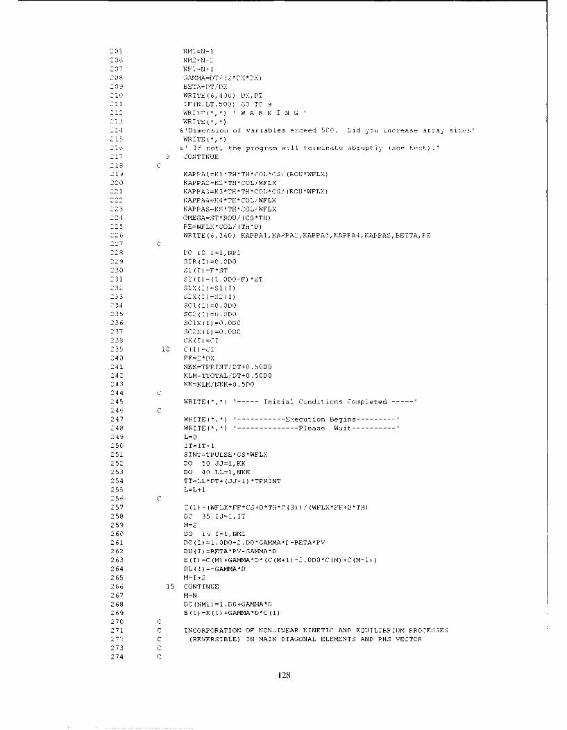
205 1~=-

20-7 NP1l=N+l208 GANM -A=DT/ 2D.X *DX)209C BETA=DT,/DX

210 WRITE(6,40u) DX,PT211 TF(N.LT.500) GO TO 9

212~~~ WA7(* R WAN I N G213 WRITE)',')

.14 &'Dimension of variables ex:ceed 500. Did y:zu increase array sizes'215 WRITE(',-)

216&' If not, the program will terminate abruptly (see te::t).217 ~ CONTINUE

218 C219 KAPPA1=KlTTTNCOL*CS/ '(ROU'WFL::)

220KAPPA2=PK'TN'COL/WFLX

221 KAPPA3=K3*TN*TN*COL*CS/ (ROU'WFLX)KAPPA4=K4*TN'COL/WFLX

223 KAPPAS=KS'*TN'COL/WFLX

24 OMEGA=ST'ROU! (CS*TN)2 5 PE=WFLX'COL1/(Th'D)

-~~ WRITE (6,340) KAPPAl, KAPPA2, KAPPA3, KAPPA4, K-APPAS ,BETTA, Pt

223PC) 10 I=1, NPlSIR) I) =0.ODO

230 S1)I)=F'ST231 52(I) = (1.000-F) 'ST

232 S 1X) I) =S1 (I)233 52-X(I)=52)(I)

234 SCl(I)=0.ODO235 5C2)1)=0).ODO

36 SC1X)I)=0.ODO-37 SC2X)I)=o0.DO

233 CX(I)=CI23910 C)I)=CI

20 F F =2 * D2:41 NKK=TPRINT/DT+0.500024 2 KLN=TTOTAL/DT+0.500024 3 KK=KLM!NKK+0.SDO244 C

25WRITE),') ------ Initial Conditions Completed ---

246C C247 WRITE),') -------- Execution Begins-----248 WRITE),') I----------Please Wait-----------249 L=O

250 IT=IT±1251 SINT=TPULSE*CS*WFLX252 DO 50 JJ=l,KK253 DO 40 LL=1,NKK254 TT=LLDT+Jj-l) *TPRINT

255 L=L+1256 C257 2)1l)=(WFLX'FF'CS+D*TN'C)3))/WFLXFF+DTN)258 DO 35 IJ=1,IT259 M=2260' DO 15 I=1,NMl261 D)=1D02D*GAMMA*E-BETA*PV

262 DU(T)=BETAP-GAMThA'D263 E)I)=CM)+GAMMhA'D' )C)N+1)-2.ODO'C)M)+C)M-1))264 DL)I) =-GANMA*D265 M=I+2266 15 CONTINUE267 M=N268 DC)NM1)=1.DO+GA4MA*D269 E)1)=E)1) +GABWAD'C)270 C271 C INCORPORATION OF NONAINFAR KINETIC AND EQUILIBRIUM PROCESSES277- C (REVERSIBLE) IN MAIN DIAGONAL ELEMENTS AND RNS VECTOR273 C274 C

128

2'75 D0 :0 1=14)81276 H1=(0..5000* (0(1+1) ±CX(I+1) ) )*(0.500* (31 (1+1) +31743*1)))

277H2=-' .50D0*(C(I+1)+CX(I+1)))*(0.SODO*(32(I+1)+S2X(I+1)()278 E(I)=E(I)-DT*(Kl*Hl-K2*(ROU/TH)*(SC1(I+1)+SC1X(I+1))/2)

279 &-DT*(K3*HN2'K4*(ROU/TH)*(SC2(T+1)+SC2X(I+1))/2')

280 C DC(I)=DC(T)-DT*KS/2

281 E(I)=E(I)-DT*(KS/1)*( (C(I+1(tCX(I+1) (/2)28220 CONTINUE

283 C284 CALL TRIDM(DC,DU,DL,E,NM1)285 DO 25 1=2,8

2 86 25 CX(I)=E(I-1)

287 CX(NP1)=CX(N)

288 CX(1)=C(1)289 DO 30 I=1,NP1

290 S1X(I)=F*ST-SC1X(I)291 S2X (I) =(1.000-F) *ST-SC2X (I)292 H1=(0.50D0*)C(I)+CX(I)))*(0.50D0*(S1(I)+S1X(I)))293 82= (0. 500* (C (I) +CX (I))) *(0. 50D0 (32 (I) +S2X (I)))294 SC1X(I)=SC1(I)+DT*(K1*(TN/ROU)*N1-K2*(SC1(I)+SCZ(I))!2)295 SC2X(I)=SC2(I)+DT*(K3*(TH/ROU)*H2-K4*(SC2(I)+SC2X(I))/2)

296 S1X(I)=F*ST-SC1X(I)297 S2X(I)=(1-F)*ST-SC2X(I)

298 SIR(I)=SIR(I)+DT*KS*(TN/ROU(*C(I)

299 30 CONTINUE300 35 CONTINUE

301 DO 36 I=1,NP1

302 C(I)=CX(I)303 S1(I)=S1X(I)304 S2(I)=S2X(I)

305 SC1(I)=SC1X(I(

306 SC2 (I) =SC2X (I)307 36 CONTINUE

308 EF=C(N)+EF

309 IF(TT.GT.TPULSE) CS=0.ODO310 40 CONTINUE

311 TIME=3J*3'PRINT

312 C

313 C

314 WRITE(6,500) TIME

315 VVO=WFLX*TIME/ (COL*TH)

316 CCO=C(N)/CO317 WRITE(6,525) VVO,CCO318 C

319 WRITE(*,650) TIME,VVO,CCO

320 WRITE (*, *) -------- Execution Continues----321 WRITE (*,* I9--------------- Please Wait-------------322 C323 WRITE(6,550)324 WRITE(6,560)325 WRITE)6,570)326 DO 45 I=1,NP1327 DEPTH=DX*(I-i)

328 45 WRITE(6,600) DEPTH,C(I),S1(I) ,S2(I),SC1(I) ,3C2(I( ,SIR))329 CALL INTEG(DX,C,X,NP1)

330 TSWATR=TH*X(NP1)

331 CALL INTEG(DX,SC1,X,NF1)

332 TS1=ROU*X(NP1(333 CALL INTEG(DX,SC2.X,NP1)

334 TS2=ROU*X(NP1)

335 CALL INTEG(DX,SIR,X,NP1)336 TSIR=ROU*X(NP1)

337 SINP=TIME*CS*WFLX

338

339 IF(SINP.GT.SINT) SINP=SINT

340 IF(CS.EQ.0.DO) SINP=SINT341 TEFFL=EF*DT*WFLX

342 BAL=(TEk'FL+TS1+TS2+TSIR+TSWATR) *100000/SINP343 WRITE (6, 200) SIN', TSWATR,T31,TS2,TSIR,TEFFL,BAL

344 50 CONTINUE

129

345 C346 100 FORMAT(/, 7X,

347 &***********************348349 & WELCOME TO

350 $//,7X,351 &1 P C V E R S I O N OF352 $//,7X,

353 &1 SECOND - ORDER TWO - SITE MODEL

354 $//,7X,

355 &1 S. 0. T. S.356 $//,7X,

357 &1 SIMULATION MODEL FOR TRANSPORT

358 $//,7X,359 &1 AND RETENTION OF HEAVY METALS IN SOILS

360 $//,7X,

361 &. UNDER STEADY - STATE WATER CONDITIONS362 $//,7X,

363

364 $/,7X,365 &1 PROGRAM WRITTEN AND DOCUMENTED

366 $/,7X,

367 &1 by

368 4$/,7X,

369 &1 H. M. SELIM370 $/,7X,371 &1 February 1990372 $/,7X,373 & *****************************************************************374

375 200 FORMAT(//,2X,'S A L T BALANCE :',//376 &7X,'TOTAL INPUT SALT FROM PULSE (MG) =',FI0.4,/377 &7X,'TOTAL SALT IN SOIL SOLUTION PHASE (MG) =',FIO.4,/,378 &7X,'TOTAL SORBED IN TYPE I SITES S1 (MG) =',FI0.4,/,

379 &7X, TOTAL SORBED IN fYPE II SITES S2 (MG) =',Fl0.4,/,380 &7X,'TOTAL SORBED IN IRREVERSIBLE PHASE (MG) =',FlO.4,/,

381 &7X,'TOTAL SALT IN THE EFFLUENT (MG) =',FIO.4,/,382 &7X,'MASS BALANCE (CALC.OUTPUT/INPUT) (%) =',F1O.4,/)

383 300 FORMAT(//,

384 $2X,'INPUT PARAMETERS :,//385 $5X,11. MOISTURE CONTENT, CM3/CM3 (TH) =',FIO.5,/386 $5X,'2. BULK DENSITY, G/CM3 (ROU) =',F10.5,/387 $5X,'3. COLUMN LENGTH, CM (COL) =',FIO.5,/

388 $5X,'4. WATER FLUX, CM/HR (WFLX) =',FI0.5,/389 $5X,'5. INITIAL CONCENTRATION, MG/L (CI) =',FI0.5,/390 $5X, '6. CONCEN. IN INPUT PULSE, MG/L (Cj) =',FlO.5,/391 $5X,'7. DISPERSION COEFFICIENT, CM2/HR (D) =',FIO.5,/392 $5X,'8. FORWARD RATE REACTION, K1,HR-I (KI) =',FI0.5,/393 $5X, '9. BACKWARD RATE REACTION, K2,HR-I (K2) =',FIO.5,/394 -4X,'10. FORWARD RATE REACTION, K3,HR-1 (K3) =',F1O.5,/395 $4X,'11. BACKWARD RATE REACTION, K4,HR-I (K4) =',F10.5,/

396 $4X,'12. FRACTION, F (F) =',FIO.5,/397 $4X,'13. TOTAL SORPTION SITES (ST) =',FIO.5,/

398 $4X,'14. IRREVERSIBLE REACTION RATE,KS,HR-1 (KS) =',FI0.5)399 310 FORMAT(

400 $4X,'15. NUMBER OF ITERATIONS (IT) =',II0,/401 $4X,'16. INPUT PULSE DURATION, HR (TPULSE) =',FIO.5,/

402 $4X,'17. TOTAL SIMULATION TIME, HR (TTOTAL) =',F10.5,/403 $4X,'18. PRINTOUT TIME DESIRED, HR (TPRINT) =',FI0.5,////)

404 340 FORMAT(//,405 $5X,'2. KAPPA1 (DIMENSIONLESS K1 ) =',FI0.5,/406 $5X,'2. KAPPA2 (DIMENSIONLESS K2 ) =',FI0.5,/

407 $5X,'3. KAPPAl (DIMENSIONLESS K3 ) =',FI0.5,/408 $5X,'4. KAPPA2 (DIMENSIONLESS K4 ) =',Fl0.5,/

409 $5X,'5. KAPPAS (DIMENSIONLESS KS ) =',FIO.5,/410 $5X,'6. OMEGA (DIMENSIONLESS ST ) =',FIO.5,/411 $5X,'7. PECLET NUMBER (WFLX*COL/D*TH) =',F0.5,///)412 400 FORMAT(2X,'THE INCREMENTS USED WERE :',//

413 $5X,'1. SIMULATION DEPTH INTERVAL,CM (DX) =',F12.6,/414 $5X,'2. INCREMENTAL TIME STEP,HR (DT) =',F12.6,///)

130

415 500 FORMAT(,'i.//,/,2X,416 $'S I M U L A T I O N T I M E (HR.) =',F8.2)417 525 FORMAT(LX,

418 $'PORE VOLUMES (V/V0) =',FI0..2,8X,'REL. CONCENTRATION (C/C0) =',419 &F8.4/)420 550 FORMAT(

421 $IX,'DEPTH',04X,'CONCENTR.',T24,'VACANT

422 $,T35,'VACANT',T45, 'FILLED'423 $,T56,'FILLED ',T67,'IRREV.')

424 560 FORMAT(425 $T24, 'SITES I',T34,'SITES II',T45,'SITES I',T56,'SITES II',426 $T67,' SINK

427 570 FORMAT(428 $2X, '(CM) ',T12,'(PPM)',T26,'(MG)',T36,'(MG)',T46,'(MG)',T57, '(MG)',429 $T68, '(MG)'!)430 600 FOPMAT(IX,F6.2,FI2.4,1X,Fl2.4,lX,F09.3,1X,F09.3,1X,F09.3,F11.3)431 650 FORMAT(i/,//,2:.:, 'SIMULATIONS ARE NOW COMPLETE UP TO',!//,5X,432 $'S I M U L A T I 0 N T I M E (HRS) =',F8.2,/!2X,433 $'PORE VOLUMES (V!V0) =',FI0.2,8X, 'REL. CONCENTRATION (C/CO)434 &F8.4//)435 700 FORMAT(50X,EI0.6)436 750 FORMAT(50X,I3)437 800 FORMAT(A64)

438 900 FORMAT(F12.0)439 950 FORMAT(Il)

440 WRITE(*,*)441 WRITE(*,*) '---- Requested Simulations Completed -

442 WRITE(*,*)443 WRITE(*,*) ' ----- SOTSPC Program Terminated Successfully ------444 WRITE(*,*)445 WRITE(*,*) .-------- THANK YOU FOR USING SOTSPC '446 END

44- C449 C

4 49 C ****

450 SUBROUTINE TRIDM(A,B,C,D,N)451 IMPLICIT REAL*8(A-H,O-Z)

452 DIMENSION A(N),B(N),C(N),D(N)453 DO 1 I=2,N454 C(I)=C(I) /A(I-1)455 A (I)=A (I)- (C(I) *B (I-1))

456 1 CONTINUE457 DO 2 I=2,N

458 D (I) =D (I) - (C (I) *D (I-1))459 2 CONTINUE

460 D (N) =D (N) /A (N)461 DO 3 I=2,N462 D (N+I1-I) = (D (N+ -I) - (B (N+1-I) *D (N+2- I) (A1N+1-I)463 3 CONTINUE464 RETURN

465 END

466 C467 C******************************************468 C SUBROUTINE INTEG PERFORMS INTEGRATION OF A TABULAR FUNCTION Y469 C GIVEN AT EQUAL DISTANCES H USING TRAPEZOIDAL RULE.470 C ********************************471 C472 SUBROUTINE INTEG(H,Y,Z,N)473 IMPLICIT REAL*8(A-H,O-Z)

474 DIMENSION Y(N),Z(N)475 S2=0.ODO476 IF(N-1) 40,30,10477 10 HH=H/2.ODO

478 DO 20 I =2,N479 Sl=S2

480 S2=S2+HH*(Y(I)+Y(I-1))481 20 Z(I-I)=Sl482 30 Z(N)=S2

483 40 RETURN

484 END

131

Sample of SOTS Model Input Data

1. MOISTURE CONTENT, CM3iCM3 (TH) = 0.400E00

2. BULK DENSITY,G/iCM3 (ROU) = 1.200E00

3. COLUMN LENGTH,CM (COL) = 10.000E00

4. WATER FLUX,CM/HR (WFLX) = 1.000E00

5. INITIAL CONCENTRATION,PPM (CI) = 0.OOOEOO

6. CONCEN.IN INPUT PULSE,PPM (CS) = 100.000E00

7. DISPERSION COEFFICIENT.,CM2/HR (D) = 1.000E00

8. TOTAL AMOUNT OF AVAILABLE SITES,ST (ST) = 166.660EOO

9. FRACTION OF TYPE I SITES, F (F) = 0.500E00

10. FORWARD RATE REACTION, K1,HR-1 (KI) = 0.007500

11. BACKWARD RATE REACTION, K2,HR-1 (K2) = 0.250E-0

12. FORWARD RATE REACTION, K3,HR-1 (K3) = 0.000750

13. BACKWARD RATE REACTION, K4,HR-1 (K4) = 0.025E-0

14. IRREVERSIBLE REACTION RATE,KS,HR-1 (KS) = 0.000E-0

15. NUMBER OF ITERATIONS (IT) 000

16. INPUT PULSE DURATION,HR (TPULSE) = 12.000E00

17. TOTAL SIMULATION TIME,HR (TTOTAL) = 16.OOOEOO

18. PRINTOUT TIME DESIRED,HR (TPRINT) 4.OOOEO0

19. INCREMENTAL TIME STEP, HR (DT) = 0.100E00

20. INCREMENTAL DISTANCE, CM (DX) = 1.000E00

132

SOTS ModelComputer Program Output Listing

WELCOME TO

PC VERSION OF

SECOND - ORDER TWO - SITE MODEL

S. 0. T. S.

SIMULATION MODEL FOR TRANSPORT

AND RETENTION OF HEAVY METALS IN SOILS

UNDER STEADY - STATE WATER CONDITIONS

****** *** ****************************

PROGRAM WRITTEN AND DOCUMENTED

by

H. M. SELIM

February 1990******************************************

INPUT PARAMETERS

1. MOISTURE CONTENT, CM3!CM3 (TH) = .400002. BULK DENSITY, G/CM3 (ROU) = 1.200003. COLUMN LENGTH, CM (COL) = 10.000004. WATER FLUX, CM/HR (WFLX) = 1.000005. INITIAL CONCENTRATION, MG/L (CI) = .000006. CONCEN. IN INPUT PULSE, MG/L (CS) = i00.000007. DISPERSION COEFFICIENT, CM2/HR (D) = 1.000008. FORWARD RATE REACTION, K1,HR-1 (0l) = .007509. BACKWARD RATE REACTION, K2,HR-1 (K2) = .25000

10. FORWARD RATE REACTION, K3,HR-1 (K3) = .00075i1. BACKWARD RATE REACTION, K4,HR-1 (K4) = .0250012. FRACTION, F (F) = .5000013. TOTAL SORPTION SITES (ST) = 166.6600014. IRREVERSIBLE REACTION RATE,KS,HR-1 (KS) = .0000015. NUMBER OF ITERATIONS (IT) = 016. INPUT PULSE DURATION, HR (TPULSE) = 12.0000017. TOTAL SIMULATION TIME, HR (TTOTAL) = 16.0000018. PRINTOUT TIME DESIRED, HR (TPRINT) = 4.00000

THE INCREMENTS USED WERE :

1. SIMULATION DEPTH INTERVAL,CM (DX) = .2500002. INCREMENTAL TIME STEP,HR (DT) = .020000

1. KAPPAI (DIMENSIONLESS K1 1.000002. KAPPA2 (DIMENSIONLESS K2 1.000003. KAPPA1 (DIMENSIONLESS K3 .100004. KAPPA2 (DIMENSIONLESS K4 .100005. KAPPAS (DIMENSIONLESS KS .000006. OMEGA (DIMENSIONLESS ST = 000007. PECLET NUMBER (WFLX*COL/D*TH) = 25.00000

133

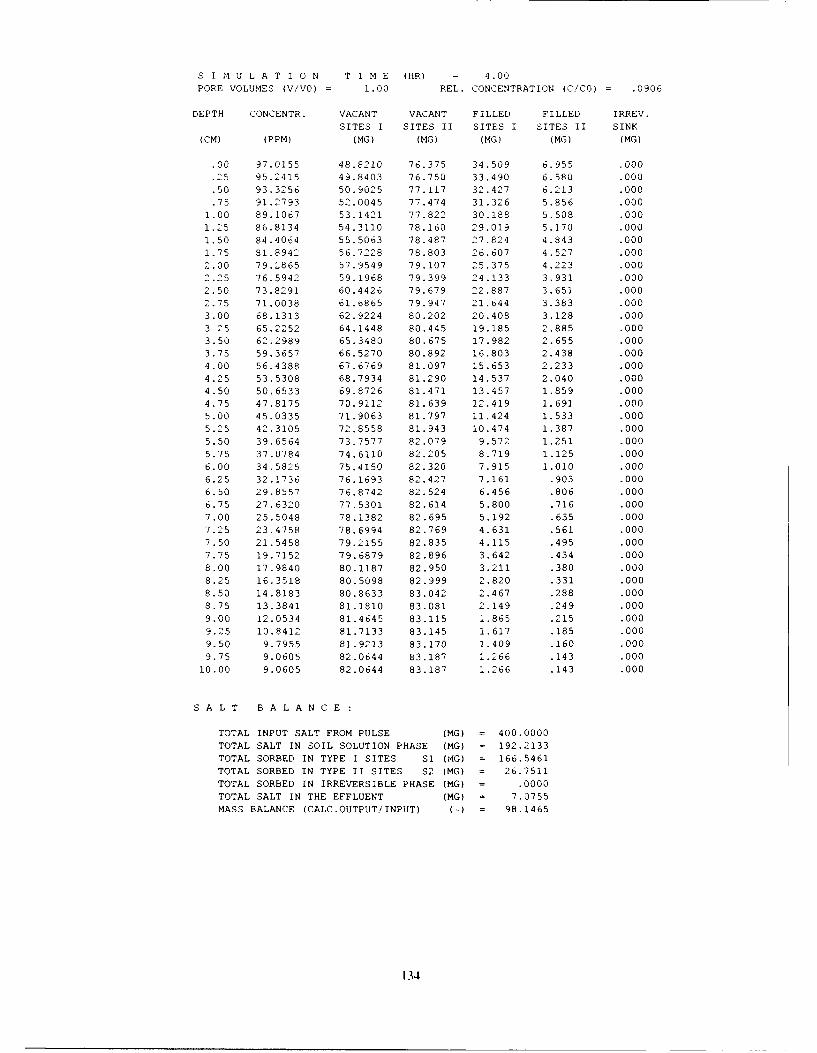
S I M U L A T I 0 N T I M E (HR) = 4.00

PORE VOLUMES (V/V0) = 1.00 REL. CONCENTRATION (C!C0) = .0906

DEPTH CONCENTR. VACANT VACANT FILLED FILLED IRREV.SITES I SITES II SITES I SITES II SINK

(CM) (PPM) (MG) (MG) (MG) (MG) (MG)

.00 97.0155 48.8210 76.375 34.509 6.955 .000

.25 95.2415 49.8403 76.750 33.490 6.580 .000

.50 93.3256 50.9025 77.117 32.427 6.213 .000

.75 91.2793 52.0045 77.474 31.326 5.856 .0001.00 89.1067 53.1421 77.822 30.188 5.508 .000

1.25 86.8134 54.3110 78.160 29.019 5.170 .000

1.50 84.4064 55.5063 78.487 27.824 4.843 .000

1.75 81.8942 56.7228 78.803 26.607 4.527 .0002.00 79.2865 57.9549 79.107 25.375 4.223 .000

2.25 76.5942 59.1968 79.399 24.133 3.931 .000

2.50 73.8291 60.4426 79.679 22.887 3.651 .0002.75 71.0038 61.6865 79.947 21.644 3.383 .000

3.00 68.1313 62.9224 80.202 20.408 3.128 .0003 25 65.2252 64.1448 80.445 19.185 2.885 .000

3.50 62.2989 65.3480 80.675 17.982 2.655 .0003.75 59.3657 66.5270 80.892 16.803 2.438 .0004.00 56.4388 67.6769 81.097 15.653 2.233 .000

4.25 53.5308 68.7934 81.290 14.537 2.040 .0004.50 50.6533 69.8726 81.471 13.457 1.859 .0004.75 47.8175 70.9112 81.639 12.419 1.691 .000

5.00 45.0335 71.9063 81.797 11.424 1.533 .000

5.25 42.3105 72.8558 81.943 10.474 1.387 .000

5.50 39.6564 73.7577 82.079 9.572 1.251 .000

5.75 37.0784 74.6110 82.205 8.719 1.125 .000

6.00 34.5825 75.4150 82.320 7.915 1.010 .0006.25 32.1736 76.1693 82.427 7.161 .903 .000

6.50 29.8557 76.8742 82.524 6.456 .806 .0006.75 27.6320 77.5301 82.614 5.800 .716 .000

7.00 25.5048 78.1382 82.695 5.192 .635 .000

7.25 23.4758 78.6994 82.769 4.631 .561 .0007.50 21.5458 79.2155 82.835 4.115 .495 .000

7.75 19.7152 79.6879 82.896 3.642 .434 .000

8.00 17.9840 80.1187 82.950 3.211 .380 .0008.25 16.3518 80.5098 82.999 2.820 .331 .000

8.50 14.8183 80.8633 83.042 2.467 .288 .0008.75 13.3841 81.1810 83.081 2.149 .249 .000

9.00 12.0534 81.4645 83.115 1.865 .215 .000

9.25 10.8412 81.7133 83.145 1.617 .185 .000

9.50 9.7955 81.9213 83.170 1.409 .160 .0009.75 9.0605 82.0644 83.187 1.266 .143 .000

10.00 9.0605 82.0644 83.187 1.266 .143 .000

SALT BALANCE:

TOTAL INPUT SALT FROM PULSE (MG) = 400.0000

TOTAL SALT IN SOIL SOLUTION PHASE (MG) = 192.2133

TOTAL SORBED IN TYPE I SITES S1 (AG) = 166.5461TOTAL SORBED IN TYPE II SITES S2 (MG) = 26.7511TOTAL SORBED IN IRREVERSIBLE PHASE (MG) = .0000TOTAL SALT IN THE EFFLUENT (MG) = 7.0755

MASS BALANCE (CALC.OUTPUTiINPUT) ( ) = 98.1465

134

S I M U L A T I 0 N T I M E (HR) = 8.00PORE VOLUMES (V/V0) = 2.00 REL. CONCENTPATION (C/C0j .3679

DEPTH CONCENTR. VACANT VACANT FILLED FILLED IRREV.

SITES I SITES II SITES I SITES II SINK(CM) (PPM) (MG) (MG) (MG) (MG) (MG)

.00 98.8940 42.9216 70.199 40.408 13.131 .000

.25 98.2309 43.2425 70.579 40.088 12.751 .000.50 97.5205 43.5881 70.957 39.742 12.373 .000.75 96.7620 43.9594 71.335 39.371 11.995 .000

1.00 95.9525 44.3575 71.712 38.973 11.618 .0001.2 5 95.089- 44.7932 72.087 38.547 11.243 .0001.50 94.1695 45.12374 72.460 38.093 10.870 .0001.75 93.1907 45.7207 72.831 37.609 10.499 .0002.00 92.1507 46.2339 73.200 37.096 10.130 .000.5 91.6474 46 .7772 73.565 36.553 9.765 .000

2.50 89.8790 47.3511 73.927 35.979 9.403 .0002.75 88.6441 47.9555 74.286 35.375 9.044 .000

3.00 87.3417 48.5903 74.640 34.740 8.690 .0003.25 85.9711 49.2553 74.990 34.075 8.340 .0003.50 84.5323 49.9499 75.335 33.380 7.995 .0003 .75 83.0256 50. 6734 75.674 32.657 7.656 .0004.00 81.4518 51.4246 76.008 31.905 7.322 .0004.25 79.8124 52.2025 76.335 31.127 6.995 .0004 .50 78.1094 53.0055 76.656 30.325 6.674 .0004.75 76.3452 53.8319 76.970 29.498 6.360 .0005.00 74.5231 54.6797 77.277 28.650 6.053 .0005.25 72.6466 55.5468 77.577 _2? 78, 5.753 ."00

5.50 70.7198 56.4310 77.868 26.899 5.462 .0005.75 63.-'474 57.3295 78.152 26.000 5.178 .0006.00 66.7345 58.2399 78.427 25.090 4.903 .0006.25 64.6864 59.1593 78.693 24.171 4.637 .0006.50 62.6090 60.0849 78.951 23.245 4.379 .00,06.75 60.5682 61.0136 79.200 22.316 4.130 .0007.00 58.3903 61.9427 79.440 21.387 3.890 .0007.25-= 56.2616 62.8691 79.671 20.461 3.659 .0007.50 54.1285 63.7899 79.892 19.540 3.438 .0007.75 51.9975 64.7023 80.105 18.628 3.225 .0008.00 49.8750 65.6035 80.308 17.727 3.022 .0008.25 47.7678 66.4;06 80.502 16.839 2.828 .0008.50 45.6834 67.3608 80.6p7 15.969 2.643 .0008.75 43.6324 68.2101 80.863 15.120 2.467 .0009.00 41.6332 69.0317 81.029 14.298 2.301 .0009.25 39.727£2 69.8103 81.182 13.520 2.148 .0009.50 38.0191 70.5055 81.316 12.824 2.014 .0009.15 36.7376 71.0067 81.411 12.323 1.919 .00010.00 36.7876 71.0067 81.411 12.323 1.919 .000

SALT BALANCE:

TOTAL INPUT SALT FROM PULSE (MG) = 800.0000TOTAL SALT IN SOIL SOLUTION PHASE (MG) = 286.2145TOTAL SORBED IN TYPE I SITES S1 (MG) = 331.2864TOTAL SORBED IN TYPE II SITES S2 (MG) = 78.3887

TOTAL SORBED IN IRREVERSIBLE PHASE (MG) = .0000TOTAL SALT IN THE EFFLUENT (MG) = 97.8128MASS BALANCE (CALC.OUTPUT/INPUT) ( = 99.2128

135

S I . U L A T I O N T I M E (HR) = 12.00PORE VOLUMES (VjV0) = 3.00 REL. CO!1CENTRATION (C/C0) = .6246

DEPTH CONCENTR. VACANT VACANT FILLED FILLED IRREV.SITES I SITES II SITES I SITES II SINK

(CM) (PPM) (MG) (MG) (MG) (MG) (MG)

.00 ?9.34L5 41.9740 65.075 41.356 18.255 .000

.25 98.9407 42.1036 65.417 41.226 17.913 .000

.50 98.5233 42.2415 65.760 41.088 17.570 .000

.75 98.0899 42.3883 66.105 40.942 17.225 .0001.00 97.6394 42.5445 66.451 40.785 16.879 .0001.25 97.1705 42.7109 66.798 40.619 16.532 .0001.50 96.6820 42.S881 67.147 40.442 16.183 .0001.75 96.1726 43.0768 67.496 40.253 15.834 .000

2.00 95.6409 43.2776 67.846 40.052 15.484 .0002.25 95.0854 43.4914 68.196 39.839 15.134 .0002.50 94.5046 43.7188 68.547 39.611 14.783 .0002.75 93.8972 43.9606 68.899 39.369 14.431 .0003.00 93.2614 44.2176 69.250 39.112 14.080 .0003.25 92.5958 44.4903 69.601 38.840 13.729 .0003.50 91.8988 44.7797 69.953 38.550 13.377 .0003.75 91.1687 45.0863 70.303 38.244 13.027 .0004.00 90.4041 45.4110 70.653 37.919 12.677 .0004.25 89.6034 45.7542 71.002 37.576 12.328 .0004.50 8.7652 46.1167 71.350 37.213 11.980 .0004.75 87.8880 46.4991 71.697 36.831 11.633 .000

5.00 86.9706 46.9017 72.042 36.428 11.288 .0005.25 86.0117 47.3252 72.385 36.005 10.945 .0005.53 85.0102 47.7699 72.725 35.560 10.605 .0005.75 83.9652 48.2361 73.064 35.094 10.266 .0006.00 82.8759 48.7239 73.399 34.606 9.931 .0006.25 81.7418 49.2335 73.732 34.096 9.598 .0006.50 80.5625 49.7650 74.061 33.565 9.269 .0006.75 79.3379 50.3181 74.387 33.012 8.943 .0007.00 78.0680 50.8927 74.708 32.437 8.622 .0007.25 76.7533 51.4883 75.026 31.842 8.304 .0007.50 75.3945 52.1045 75.339 31.225 7.991 .000

7.75 73.9926 52.7406 75.647 30.589 7.683 .0008.00 72.5490 53.3957 75.950 29.934 7.380 .0008.25 71.0661 54.0687 76.247 29.261 7.083 .0008.50 69.5475 54.7578 76.539 28.572 6.791 .000

8.75 68.0006 55.4598 76.824 27.870 6.506 .0009.00 66.4412 56.1679 77.100 27.162 6.230 .0009.25 64.9079 56.8658 77.362 26.464 5.968 .0009.50 63.4983 57.5102 77.596 25.820 5.734 .0009.75 62.4646 57.9857 77.765 25.344 5.565 .000

10.00 62.4646 57.9857 77.765 25.344 5.565 .000

S A L T B A L A N C E :

TOTAL INPUT SALT FROM PULSE (MG) = 1200.0000TOTAL SALT IN SOIL SOLUTION PHASE (MG) = 337.7995

TOTAL SORBED IN TYPE I SITES S1 (MG) = 422.0256TOTAL SORBED IN TYPE II SITES S2 (MG) = 137.2232TOTAL SORBED IN IRREVERSIBLE PHASE (MG) = .0000

TOTAL SALT IN THE EFFLUENT (MG) = 299.4983

MASS BALANCE (CALC.OUTPUT/INPUT) (') = 99.7122

136

S I M U L A T IO N T I M E (HR) 16.00

PORE VOLUMES (V/VO) = 4.00 REL. CONCENTRATION (C/CO) .5845

DEPTH CONCENTR. VACANT VACANT FILLED FILLED IRREV.

SITES I SITES II SITES I SITES II SINK

(CM) (PPM) (MG) (MG) (MG) (MG) (MG)

.00 2.2278 66.3619 66.380 16.968 16.950 .000

.25 3.5953 65.3925 66.438 17.938 16.892 .000

.50 4.9921 64.4567 66.504 18.873 16.826 .000

.75 6.4113 63.5539 66.578 19.776 16.752 .0001.00 7.8512 62.6834 66.660 20.647 16.670 .000

1.25 9.3098 61.8445 66.749 21.485 16.581 .0001.50 10.7853 61.0368 66.846 22.293 16.484 .0001.75 12.2761 60.2596 66.951 23.070 16.379 .000

2.00 13.7806 59.5126 67.063 23.817 16.267 .000

2.25 15.2972 58.7955 67.183 24.535 16.147 .000

2.50 16.8245 58.1078 67.310 25.222 16.020 .0002.75 18.3611 57.4493 67.444 25.881 15.886 .0003.00 19.9058 56.8199 67.586 26.510 15.744 .0003.25 21.4575 56.2194 67.734 27.111 15.596 .0003.50 23.0151 55.6479 67.890 27.682 15.440 .000

3.75 24.5776 55.1052 68.052 28.225 15.278 .0004.00 26.1442 54.5914 68.221 28.739 15.109 .000

4.25 27.7141 54.1068 68.397 29.223 14.933 .0004.50 29.2868 53.6515 68.579 29.679 14.751 .000

4.75 30.8615 53.2257 68.767 30.104 14.563 000

5.00 32.4375 52.8298 68.962 30.500 14.368 .000

5.25 34.0143 52.4642 69.163 30.866 14.167 .0005.50 35.5909 52.1293 69.370 31.201 13.960 .0005.75 37.1661 51.8256 69.583 31.504 13.747 .000

6.00 38.7385 51.5537 69.801 31.776 13.529 .000

6.25 40.3060 51.3141 70.025 32.016 13.305 .0006.50 41.8662 51.1074 70.255 32.223 13.075 .0006.75 43.4157 50.9342 70.490 32.396 12.840 .0007.00 44.9502 50.7951 70.729 32.535 12.601 .000

7.25 46.4648 50.6907 70.974 32.639 12.356 .000

7.50 47.9534 50.6214 71.223 32.709 12.107 .0007.75 49.4088 50.5879 71.476 32.742 11.854 .000

8.00 50.8232 50.5904 71.734 32.740 11.596 .000

8.25 52.1875 50.6290 71.995 32.701 11.335 .000

8.50 53.4920 50.7037 72.259 32.626 11.071 .000

8.75 54.7261 50.8134 72.525 32.517 10.805 .000

9.00 55.8764 50.9553 72.790 32.375 10.540 .0009.25 56.9223 51.1223 73.048 32.208 10.282 .000

9.50 57.8190 51.2964 73.284 32.034 10.046 .0009.75 58.4450 51.4343 73.457 31.896 9.873 .000

10.00 58.4450 51.4343 73.457 31.896 9.873 .000

SALT BALANCE:

TOTAL INPUT SALT FROM PULSE (MG) = 1200.0000TOTAL SALT IN SOIL SOLUTION PHASE (MG) = 128.5387

TOTAL SORBED IN TYPE I SITES S1 (MG) = 341.2330

TOTAL SORBED IN TYPE II SITES S2 (MG) = 167.7559TOTAL SORBED IN IRREVERSIBLE PHASE (MG) = .0000

TOTAL SALT IN THE EFFLUENT (MG) = 568.6738

MASS BALANCE (CALC.OUTPUT/INPUT) (%) = 100.5168

137

APPENDIX D: SOMIM

Computer Program Listing

1 C2 $LARGE

3 *****************************

4 C C

5 C S************* . 0. M. I. M. ********** C6 C C7 C SECOND - ORDER MOBILE - IMMOBILE MODEL C

8 C C

9 C'**************************************************10 C C11 C COMPUTER PROGRAM C

12 C C

13 C FOR THE TRANSPORT AND RETENTION OF HEAVY METALS IN SOILS C

14 C C15 C UNDER STEADY - STATE WATER FLUX CONDITIONS C

16 C C

17 C USING C18 C C19 C THE CONVECTIVE - DISPERSIVE EQUATION C

20 C C21 C WITH THE MOBILE - IMMOBILE WATER CONCEPT C

22 C C23 C WITH C24 C C25 C REVERSIBLE SECOND - ORDER KINETICS AND IRREVERSIBLE REACTIONS C26 C C

27 *************************** **********r*******************28 C C29 C PROGRAM WRITTEN AND DOCUMENTED C

30 C C

31 C by C32 C C33 C H. M. SELIM C

34 C February 1990 C

35 C'******************************************36 C C

37 IMPLICIT REAL*8(A-H,O-Z)38 CHARACTER*64 FNAMEI,FNAMEO

39 DIMENSION DC(501),DU(501),DL(501),E(501),CM(501),CIM(501)

40 DIMENSION CMX(501),CIMN(501)41 DIMENSION SIR(501),SM(501),SMX(501),SIM(50142 CHARACTER*64 USER, SOIL, SOLUTE, DATE

43 REAL*8 K1,K2,KS,KAPPAI,KAPPA2,KAPPAS

44 C

45 C46 WRITE(*,100)

47 C --- READ INPUT PARAMETERS----------------

48 C49 WRITE(*,*) ' PLEASE ENTER USER NAME (OPTIONAL):'

50 READ(*,800) USER51 WRITE(*,*) ' PLEASE ENTER NAME OF SOIL (OPTIONAL):'

52 READ(*,800) SOIL53 WRITE(*,*) ' PLEASE ENTER NAME OF SOLUTE (OPTIONAL):'

54 READ(*,800) SOLUTE55 WRITE(*,*) ' ENTER DATE OR OTHER IDENTIFICATION (OPTIONAL)

56 READ(*,800) 53 DATE

57 WRITE(*,*)

58 WRITE(*,')59 $' -------- INPUT PARAMETERS SECTION -

60 WRITE(*,*) ' '

61 WRITE(*,*) ' INPUT PARAMETERS CAN BE PROVIDED IN TWO WAYS;'62 WRITE(*,*) ' ENTER 1 if you wish to enter the input data using'

63 WRITE(*,*) ' the keyboard (i.e. interactively)'

64 WRITE(*,*)

139

65 WRITE(*,*) ' OR'

66 WRITE(*,*)

67 WRITE(*,*) ' ENTER 2 if an input data file is to be provided'

68 WRITE(*,*)69 $' PLEASE ENTER EITHER 1 OR 2'

70 READ(*,950) IFLAG71 IF(IFLAG.NE.I) THEN

72 WRITE(*,1(A)1) ' PLEASE ENTER NAME OF INPUT FILE?'73 WRITE(*,*) '(for example A:XX.DAT or C:UU.DAT for hard disk)'

74 READ(*, '(A) ') FNAMEI75 OPEN(5,FILE=FNAMEI)76 C77 READ(5,700) TH,ROU,COL,WFLX

78 READ(5,700) CI,CS,D,ST,F,FTH

79 READ(5,700) KI,K2,KS,TR

80 READ(5,750) IT

81 READ(5,700) TPULSE,TTOTAL,TPRINT,DT,DZ

82 C

83 ELSE

84 C

85 WRITE(*,*)Z_ $'PLEASE ENTER THE FOLLOWING INPUT PARAMETERS

87 WRITE(*,*)

88 WRITE(*,*)89 $' (1) MOISTURE CONTENT,CM3/CM3 (TH) ='

90 WRITE(*,*)91 $' (Values usually less than 0.65 cm3/cm3). Enter your value NOW'92 READ(*,900) TH

93 WRITE(*,*)94 $' (2) BULK DENSITY,G/CM3 (ROU)

95 WRITE(*,*)

96 $' (Range of values 1.1 - 1.7 g/cm3). Enter your value NOW'

97 READ(*,900) ROU98 WRITE(*,*)99 $' (3) COLUMN LENGTH (CM) (COL) ='100 READ(*,900) COL

101 WRITE(*,*)102 $' (4) WATER FLUX (CM/HR) (WFLX) -'

103 WRITE(*,*)104 $'(Range of values 0.01 - 5 cm/hr). Enter your value NOW'105 READ(*,900) WFLX

106 WRITE(*,*)

107 $' (5) INITIAL CONCENTRATIO, (CI)108 READ(*,900) CI109 WRITE(*,*)110 $' (6) APPLIED CONCENTRATION, (CS)

i1l READ(*,900) CS

112 WRITE(*,*)113 $' (7) DISPERSION COEFFICIENT, (CM2/HR) (D) -'

114 WRITE(*,*)

115 $'(Range of values 0.1 - 1.5 cm2/hour). Enter your value NOW'116 READ(*,900) D

117 WRITE(*,*)

118 $' (8) TOTAL SORPTION SITES (ST) ='

119 READ(*,900) ST

120 WRITE(*,*) '(Ranges from 200 to 2000 mg/kg). Enter your value NOW'

121 WRITE(*,*)122 $' (9) FRACTION OF SITES, F (F) ='

123 WRITE(*,*) '(Ranges from 0.0 to 1.0). Enter your value NOW'124 READ(*,900) F

125 WRITE(*,*)

126 $' (10) FRACTION OF MOBILE WATER, FTH (FTH) -'

127 WRITE(*,*) '(Ranges from 0.1 to 1.0). Enter your value NOW'128 READ(*,900) FTH

129 WRITE(*,*)

130 $' (11) FORWARD RATE REACTION, KI,HR-1 (Kl) -'

131 WRITE(*,*) '(Ranges from 0.001-0.1 hr-i). Enter your value NOW'132 READ(*,900) K1

133 WRITE(*,*)134 $' (12) BACKWARD RATE REACTION, K2,HR-1 (K2)

140

135 WRITE(',* '( Ranges from 0.0 - 7.2 hr -11- Enter your value NIX'13 0 F.EAD(-, 1) K?13- WRITE,,*

13$ S' (13) IRFEVERSIELE REA7TION RATEKS,HF-1 (KS)13 WRITE(,-)

140 WRITE(',*) 'tRange is 0.0301 - 0.5 hr-1 Enter your value NOW'141 FEAl)', SO0 KS

141 WRITE(-,-)143 V' (14) MASS TRANSFER COEFFICIENT,TR, HR-I )TR)

144 WRITE(*,*) '(Range is 0.01 - 0.1 hr-i). Enter your value NOW'145 REAL 1, 00) TR140 WRITE(-,-)

147 $1 (1S) NrUMOE OF ITERATIONS (IT) (Integer value from I to14' READ) Q950) IT149 WRITE(',')

10i V' 15) INPUT PULSE DURATION,NR )TPULSE)151 READ)', 00) TPULSE

151 WRITE,')153 V' (17) TOTAL SIMULATION TIME, HR (TTOTAL)154 READ)', 90K) TTOTAL

155 WRITE(-,-)155 $' (13) PRINTOUT TIME DESIRED,HR (TPRI'AT)

Is- rEn~t,,Y60) TERINT15? WRITE(',-)

13V (19) INCREMENTAL DISTANCE, CM )D7) -

!&:) WRITE)-,*)1i $ A default value of DZ=1.00 is given

16 READ)',900) DDZ16 WRITE)',')

36 ' (20) INCREMENTAL TIME STEP, HR. )DT) -

iW5 WRITE),')16- $' A default value of Dt=0.0: is given

ij-READ), 00) DDT16? ENDIF

17 1 IF(DDS.NE.0.0) THEN

1--, DZ=DD2173 ELSE

-4 DI=I IN175 ENDIF

1. PIN=0 .01177 IF)DDT.NE.0.0) THEN

DT= DDT1 ELSE18" DT=P III

M END IF182 C

1?3WRITE),')A) ') * LEASE ENTER NAME OF OUTPUT FILE (FOP EXAMPLE184 E:ZZ.DAT)'

135 READ)(*, ' (A) ') FNAMKEO

136 OPEN (6, FILE=FNAMEO, STATUZS 'UNYNOWN')

130 WRITE)6,100)i i,: WRITE)E,30) USER

190 WPITE)6,800( SOIL19i WRITE(6, 300) SOLUTE

191 WRITE)6,?00) lATE

193 WRITE)5,300) TH,POU,COL,WFLX,CI,CS,D,ST,F,FTH,K 1,KIF,TP

134 WRITE6, 310) IT,TPULSE,TTOTAL,TPPINT195 C

197

103 THM=TH"FTH

19 THIM=TH-THM100 P'ThWFLX/THM~

101

103 FA!PA2-KI TH'COL'WFLX104 KAPPAS=KS'TH'COLiWFLX

141

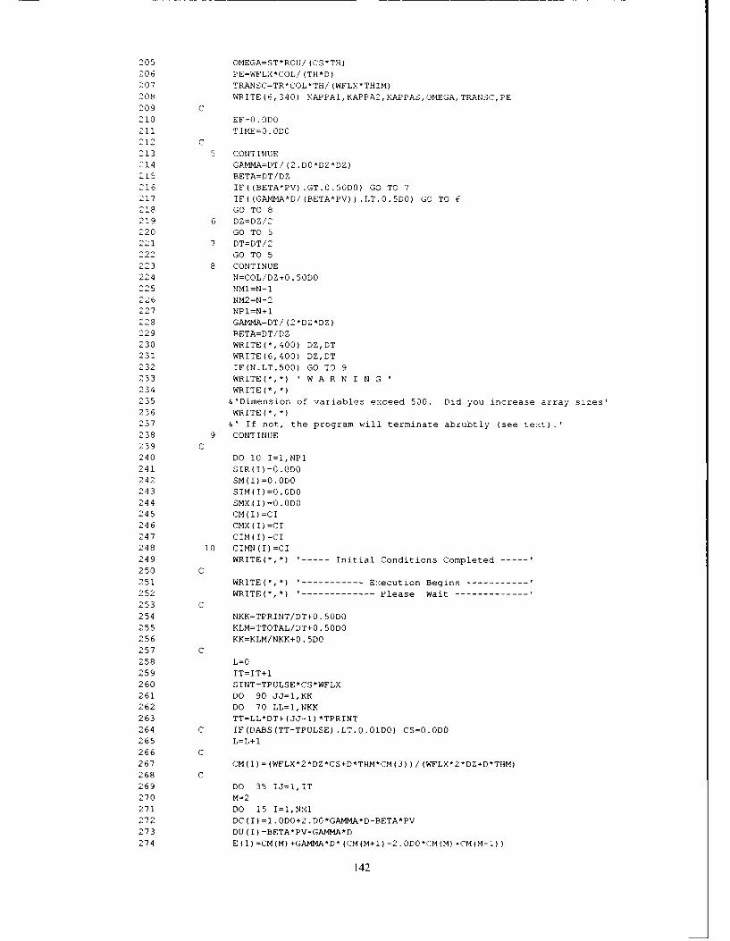
2 05 OMEGA=ST*ROU/ (CS*TH)

206 PE=WFLX*COL/(TH*D)207 TRANSC=TR*COL*TH'/ (WFLX*THIM)

208WRITE(6, 340) KAPPAl,KAPPA2-,KAPPAS,OMNEGA,TRANISC,PE209 C

210 EF=O.0D0

211 TIME=O.0D0212 C

213 5 CONTINUE2 14 GPMMA=DT/(2'.D0*DZ*DZ)

215 BETA=DT/DZ216 IF((BETA*PV).GT.0.50D0) GO TO 7217 IF((GAt4MA*D/(BETA*PV)).LT.0.5DO) GO TO 6218 GO TO 8

2119 6 DZ=DZ/22120 GO TO 5

221 7 DT=DT/2

2222 GO TO 52213 8 CONTINUE

224 N=COL/DZ+0. SODO225 NM1=N-l

226 NM2=N-2227 NPl=N+l228 GAM4MA=DT/ (2*DZ*DZ)

229 BETA=DT/DZ230 WRITE(*,400) DZ,DT231 WRITE(6,400) DZ,DT

232 IF(N.LT.500) GO TO 9233 WRITE(*,*) -W A R N I N G234 WRITE(*,*)235 &'Dimension of variables ex.ceed 500. Did you increase array sizes'2316 WRITE(*,*)

237 &1 If not, the program will terminate abrubtly (see te::-t).238 9 CONTINUE239 C240 DO 10 I=1,NP1

241 SRI=.D

242 SM(I)=0.ODO

243 SIM(I)=0.ODO

244 SMX(I)=0.ODO245 CM(I)=CI246 CMX(I)=CI247 CIM(I)=CI248 10 CIMN(I)=CI249 WRITE(*,*) ------ Initial Conditions Completed---

250 C251 WRITE(*, *)--------------- E::ecution Begins-------------252 WRITE (*, *)------------------ Please Wait----------------I253 C254 NKK=TPRINT/DT+0. SODO255 KLM=TTOTAL/DT±0. SODO256 KK=KLM/NKK+0. SDO257 C258 L=0259 IT=IT4-1260 SINT=TPULSE*CS*WFLX261 DO 90 JJ=1,KK262 DO 70 LL=1,NKK263 TT=LLDT+(,JJ-1) *TPRINT264 C IF(DABS(TT-TPULSE) .LT.01DO) CS=0.ODO265 L=L+1266 C267 CM(1)=(WFLX*2*DZ*CS+D*THM*CM(3))/(WFLX*2*DZ+D*THM)268 C269 DO 35 IJ=1,IT270 M=1

271 DO 15 I=1,N!/1272 DC(I)=l.D+2.D*GAMMA*D-BETA*PV273 DU(I)=BETA*PV-GAMMA*D274 E(I)=CM(M)+GAMMA*D*(CM(M+1)-2.0D0CM(M) +CM(M-1))

142

275 DL(I)=-GAMM1A*D276 M=I+2277 15 CONTINUE278 M=N279 DC(NM1)=l.DO+GA34A*D280 E(1)=E(1)+GAMMA*D*CM(l)

281 C282 Do 20 I=1,NM1283 M=I+1284 P8IM=F'ST-SM(M)285 PHIMX=F*ST-SMX (N)286 PHIIM=(1.0D0-F)-ST-SIM(N)287 H1=((CM(M)+CMX(N))/2)*((PHIM+PHIMX)/2)288 RK<M=Kl*THM*H1.K2*ROU*(SM(M)+SMX(M) )/2289 RKM=RKM*F*DT/TiHM290 RIN=Kl*THIM*CI (N) *PHIIMNROU*K2*SIM (N)291 RKIM=(l.ODO-F) *DT*RKIM/T(M292 E(I)=E(1)-RKM-RKIM293 E(I)=E(I)-(CIMN(N-)-CIM(M))*(THIM/THM)294 C E(I)=E(I)-DT*Ks*((CM(N)+CMX(M))/2)-DT*KS*(THI/TH)*CIM(M;295 E(I)=E(I)-DT*KS*((CM(M)+CX() )/2)296 20 CONTINUE297 CALL TRIDM(DC,DU,DL,E,NMI)298 DO 25 I=2,N299 25 CMX(I)=E(I-1)300 CMX(NP1)=CMX(N)301 CMX(1)=CM(1)302 DO 30 I=1,NP1303 PHIM=F*ST-SM(I)304 PHIMX=F*ST-SMX(I)305 Hl=((CM(I)+CMX(I))/2)*((PHIM+PHIMX)/2)306 SMX(I)=SM(I)+DT*307 &(K1*(THM/ROU)*H1-K2*(SM(I)+SMX(l))/2)308 30 CONTINUE309 35 CONTINUE310 DO 40 I=1,NP1311 40 CIM(I)=CINN(I)312 DO 45 I=1,N313 PHIIM=(l.0D0-F)*ST-SIM(I)314 RKIM=K1*THIM*CIM(I) *PHIIM.ROU*K2*SIM(I)315 RKIM=(1.ODO-F) *DT*RKIM/THIM316 CIMN(I)=CIM(I)-RKIM+317 &DT*(TR/THIM)*(CMX(I)-CIM(I))318 &-DT*KS*CIM(I)

319 H2=CIMN(I)*PHIIM320 SIM(I)=SIM(I)+DT*321 & (K1* (T1IM/ROU) *H2..K2*SIM(I))322 45 CONTINUE323 SIM(NPI)=SI4(N)324 CIMN(NP1)=CIMN(N)325 DO 50 I=1,NP1326 SIR(I)=SIR(I)+DT*KS/ROU*(THiM*CM(I)+THIM*CIM(I))

32'7 CM(I)=CMX(I)328 SM(I)=SMX(I)329 50 CONTINUE

330 EF-CM(N)+EF331 IF(TT.GT.TPULSE) CS-0.0D0332 70 CONTINUE333 TIr4E=JJ*TPRINT334 C335 WRITE(6,500) TIME336 VV0=WFLX*TIM~E/ (COL*TH)337 CCO=CM(N)/CO338 WRITE(6,525) VVO,CCO339 WRITE(*,650) TIMEW10,CC0340 W~RITE(*,*) -----------Execution Continues----341 WRITE(*, *)----------------- Please Wait-------------342 C343 WRITE(6,550)344 WRITE(6,560)

345 WPI TR( S7346 0 =,CR

'47 5=E0% 1-1

343 STX=SM(I( T±+ S (I) 31F, (I)

350I CAL INEODSZC-mEN -T'

351 SMW;=TNM'E (11P)35-AL-L INTEG (OSZ, MI, E, NP 1353TSIM7V=TMIM'E (NIP1

354CALL IN:TEG(DZ,SM,,E,NP1)

3-55 TMRUFE(M3156 CALL 1INTEG(-DZ, SIM,E,NP1)

357 TI=Ot(.D-(EN1

-* ALL ITES (DS, 31R., E,NP 1)T S:R=FrOUE (NPI)

360 SINJP=TIIIE*CS*WFLX

362 IF(SINIP.GT.STNT) SINP=SINT3,63 IF(CS.EQ.0O.DOj SINP=SINIT3164 TEFFL=EF*DT*WFLZjo5 TSW=TSIMW±TSMW

366 BAL=(TEFFL+TSWsTSIRsTS-rTSIM) *TOOODO/-ZIN;P367 WITE(6,200) SIN;P,TSM4W,TSIM4W,TSM f,TSIM,TSIR,TEFFL,B-AL

00i CONTINUE369 10 0 FORMAT)!!,, 7/Z,

3-71 3/ 1Z7372 - WELCOME TO373 3 A

374 a P C VERSION OF

3% & SECOND - ODER MO0BILE - IMM4OBILE MODEL

077,

330 S IMULATION MODEL FOR TRANSPORT

AN[ RETENTION OF MEAVY IdETALS- IN SOI LS

334 &' UNDER STEADY -STATE NATER CONDI;[,TIONS

333 & PROGRAM WRITTEN AND DOCUMENTED

390i, &. by

392&'H. M. SELIMS,/, 77,

304 9February I~

33 20 G0 FORM4AT '-,X,'Sz A L T B A L AN C E :,30 -X7, 'TOTAL INPUT SALT FROM PULSE (MG)='F .4/

400r -7X, 'TZOTAL SALT 11N MOBILE-WATER PHASE (MG) =', F1O.4, I,401 i7Z, ITOTAL. SALT INI IIa24OBILE-WATER PHASE (MG) =',O.,,

402 'P7X,'TOTAL SRPBED IN MOBILE PHASE SM (MG) =' ,F1O.4,,403 ,7X, 'TOjTAL SORBED INl IMM4OBILE PHASE SIM (MG) =',F' 1.,i

404 &7X, 'TOTAL SORBED INI IRREVERSIBLE PHASE (MG) =',F1O.4, 7,

405 &AX, 'TOTAL SALT IN4 THE EFFLUENT (MG) =' ,F1O.4_,!

406 'AX, 'MASS BALANCE (CALC.OUTPUT/INPUT) ()=',F10.4,!/)

407 30 0 FORM4AT)!/!,40r3 527, -'INPUT PARAM4ETERS :',/400 9 SX, '1. MOISTURE CONTENT, CM3/CM3 (TN) - l41(0 57z,'2. RULE DENSITY, G/C:13 (ROJ ',1.5411 ""X, '3 OLUMN LENGTH, CM (COL) F'1'Ri. 5,;4 12 557., '4. WATER FLUX, CM/HR (WJFLX( =',FIO.5,/

413 S57, 5. INITIAL CONCENTRATION, MG!L (.-I) ='F1O.5,,

414 SIX., '6. COINCEN. IN INPUT PULSEF, 14WL ('C) = ',F10.5_/

144

415 $5X, '7. DISPERSION COEFFICIENT, CM2iHR (D) -'

416 $5X, '8. TOTAL SORPTION SITES (ST ',F10.5,'

417 $5X, 9. FRACTION OF SITES, F (F) =',FI0.5,-418 $4X, 10. FRACTION OF MOBILE WATER, FTH (FTH) =',FIO.5,419 $4X, 11. FORWARD PATE REACTION, KI,HR-1 (KI) ='F05

420 $4X,'12. BACKWARD RATE REACTION, K2,HP-1 (K2) =,FI0.5421 $4X,'13. IRREVERSIBLE REACTION RATE,KS,HR-1 (KS) =',FI0.5,

422 $4X, 14. MASS TRANSFER COEFFICIENT,TR, HR-i (TR) =-',F0.5)423 310 FORMAT(

424 $4X, '15. NUMBER OF ITERATIONS ::',IlOi425 $4X,'16. INPUT PULSE DURATION,HR (TPULSEi =',FI0.5,'

426 $4X,'17. TOTAL SIMULATION TIME,HR (TTOTAL) =',FlO.5,!427 $4X, '18. PRINTOUT TIME DESIRED,HR (TPRINT) =',F10.5,!!!/)428 340 FORMAT(/

429 $5X, 'I. KAPPAl (L .NSIONLESS '1 ) =',F10.5,1430 $5X, '2. KAPPA2 (DIMENSIONLESS K2 ( =',F10.5,/

431 $5X,'3. KAPPAS (DIMENSIONLESS KS )432 $5X, '4. OMEGA (DIMENSIONLESS ST =',FIO.5,/433 $5X,'5. TRANSFER COEFFICIENT (DIMENSIONLESS) =',FI0. ,/

434 $5X,'6. PECLET NUMBER (WFLX*COL,/D*TH) =',FI0.5,///)435 400 FORMAT(2X,'THE INCREMENTS USED WERE :',//436 $5X, '1. SIMULATION DEPTH INTERVAL, CM (DZ) =',F12.6,/437 $5X,'2. INCREMENTAL TIME STEP, HR (DT) =',F12.6,///)

438 500 FORMAT(////////, 2X,439 $'S I M U L A T I 0 N T I M E (HR) =',F8.2)440 525 FORMAT(2X,441 $'PORE VOLUMES (V/VO) =',F0.2,8X, 'REL. CONCENTRATION (C/C0)442 &F8.4/)

443 550 FORMAT(444 $1X,'DEPTH',06X,'CONCENT.',T25,'CONCENT.'

445 $,T36,'SORBED',T47,'SORBED'446 $,T56,'IRREVERS',T67,'TOTAL')

447 560 FORMAT(12X,'MOBILE',

448 $T25,'IMMOBILE',T36,'MOBILE',T46,'IMMOBILE',T58,'SINK',

449 $T67,'SORBED')

450 570 FORMAT(2X,'(CM)',TI3,'(PPM)',T26,'(PPM)',T37,'(MG)',T48,'(MG)',

451 $T59,'(MG) ,T68,'(MG)'/)452 600 FORMAT(lX,F6.2,FI2.4,1X,F12.4,1X,F09.3,lX,F09.3,1X,F09.3,Fll.3)

453 650 FORMAT(////,2X,'SIMULATIONS ARE NOW COMPLETE UP T-',//!,5X,

454 $'S I M U L A T I 0 N T I M E (HR) =',F8.2,//2X,455 $'PORE VOLUMES (V/V0) =',FI0.2,8X,'REL. CONCENTRATION (C/C0)

456 &F9.4//)457 700 FORMAT(50X,E10.6)

458 750 FORMAT(50X,I3)

459 800 FORMAT(A64)460 900 FORMAT(F12.0)

461 950 FORMAT(I1)

462 WRITE(*,*)463 WRITE(*,*) '------ Requested Simulations Completed -------

464 WRITE(*,*)465 WRITE(*,*) '------ SOMIMPC TERMINATED SUCCESSFULLY --------466 WRITE(*,*)

467 WRITE(*,*) --------- THANK YOU FOR USING MIMPC -------------468 END469 C

470 C471 C472 C

473 SUBROUTINE TRIDM(A,B,C,D,N)474 IMPLICIT REAL*8(A-H,O-Z)475 DIMENSION A(1),B(1),C(1),D(1)476 DO 1 I=2,N477 C(I)=C(I)/A(I-I)

478 A(I)=A(I)-(C(I)*B(I-I))

479 1 CONTINUE480 DO 2 I=2,N

481 D(I)=D(I)-(C(I)*D(I-1))

482 2 CONTINUE483 D(N)-D(N)/A(N)

484 DO 3 I=2,N

145

485 0 (N+1-I) =(D (N+1-I) -(B (N+1-I) *D (N+2--I) )) !A(N+1-1)

436 3 CONTINUE

487 RETURN

438 END

489 C

490 SUBROUTINE INTEG(H,Y,Z,N)

491 IMPLICIT REAL*8(A-N,O-Z)

492 DIMENSION Y(N),Z(N)

493 S2=0.ODO

494 IF(N-1) 40,30,10

495 10 HN=N/'2.ODO

496 DO 20 1 =2,N

497 51=52"

498 S2=S2+N4* (Y(I)+Y(I-1))

499 20 Z(I-1)=S1

500 30 Z(N)=S2

501 40 RETURN

502 END

146

Sample of SOMIM Input Data

1. MOISTURE CONTENT,CM3/CM3 (TH) = 0.400E002. BULK DENSITY,G/CM3 (ROU) = 1.200E003. COLUMN LENGTH,CM (COL) = 10.000E004. WATER FLUX,CM/HR (WFLX) = 1.000E005. INITIAL CONCENTRATION,MG/L (CI) = 0.000E006. CONCEN.IN INPUT PULSE,MG/L (CS) = 100.000E007. DISPERSION COEFFICIENT,CM2/HR (D) = 1.000E008. TOTAL ST (ST) = 166.660E009. FRACTION OF SITES, F (F) = 0.500EOO10. FRACTION OF WATER, FTH (FTH) = 0.500E0011. FORWARD RATE REACTION, KI,HR-1 (KI) = 0.00750012. BACKWARD RATE REACTION, K2,HR-I (K2) = 0.250E-013. IRREVERSIBLE REACTION RATE,KS,HR-1 (KS) = 0.000E-014. TRANSFER COEFFICIENT, TR (TR) = 0.050E-015. NUMBER OF ITERATIONS (IT) = 00016. INPUT PULSE DURATION,HR (TPULSE) = 12.OOEOO17. TOTAL SIMULATION TIME,HR (TTOTAL) = 16.00E0018. PRINTOUT TIME DESIRED,HR (TPRINT) = 4.OOEOO19. INCREMENTAL TIME STEP, HR (DT) = 0.10EOO20. INCREMENTAL DISTANCE, CM (DZ) = 1.00E00

147

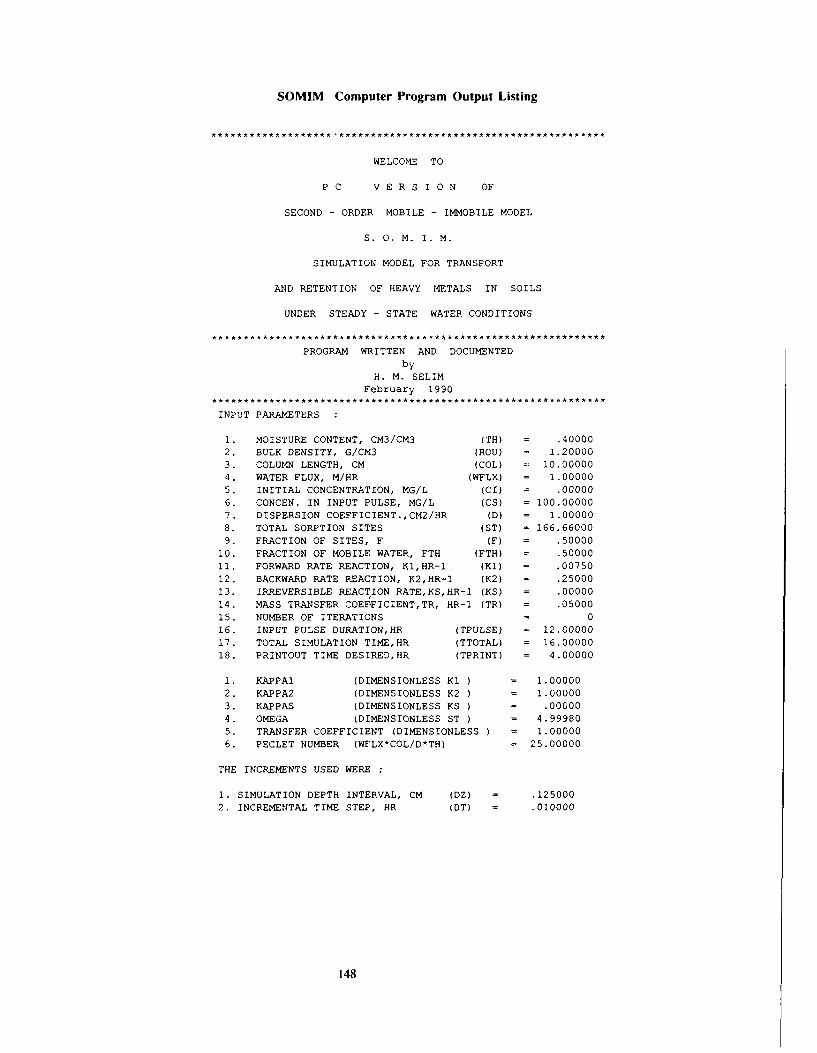
SOMIM Computer Program Output Listing

WELCOME TO

PC VERSION OF

SECOND - ORDER MOBILE - IMMOBILE MODEL

S. 0. M. I. M.

SIMULATION MODEL FOR TRANSPORT

AND RETENTION OF HEAVY METALS IN SOILS

UNDER STEADY - STATE WATER CONDITIONS

**************************** **********************************

PROGRAM WRITTEN AND DOCUMENTEDby

H. M. SELIM

February 1990

INPUT PARAMETERS

1. MOISTURE CONTENT, CM3/CM3 (TH) = .40000

2. BULK DENSITY, G/CM3 (ROU) = 1.20000

3. COLUMN LENGTH, CM (COL) 10.000004. WATER FLUX, M/HR (WFLX) = 1.00000

5. INITIAL CONCENTRATION, MG/L (CI) .00000

6. CONCEN. IN INPUT PULSE, MG/L (CS) = 100.000007. DISPERSION COEFFICIENT.,CM2/HR (D) = 1.00000

8. TOTAL SORPTION SITES (ST) = 166.660009. FRACTION OF SITES, F (F) = .50000

10. FRACTION OF MOBILE WATER, FTH (FTH) = .50000

11. FORWARD RATE REACTION, KI,HR-1 (Ki) .00750

12. BACKWARD RATE REACTION, K2,HR-1 (K2) = .25000

13. IRREVERSIBLE REACTION RATE,KS,HR-1 (KS) = .00000

14. MASS TRANSFER COEFFICIENT,TR, HR-1 (TR) = .05000

15. NUMBER OF ITERATIONS - 0

16. INPUT PULSE DURATION,HR (TPULSE) 12.00000

17. TOTAL SIMULATION TIME,HR (TTOTAL) = 16.00000

18. PRINTOUT TIME DESIRED,HR (TPRINT) = 4.00000

1. KAPPA1 (DIMENSIONLESS K1 ) 1.00000

2. KAPPA2 (DIMENSIONLESS K2 ) 1.00000

3. KAPPAS (DIMENSIONLESS KS ) = .000004. OMEGA (DIMENSIONLESS ST ) = 4.99980

5. TRANSFER COEFFICIENT (DIMENSIONLESS) = 1.00000

6. PECLET NUMBER (WFLX*COL/D*TH) = 25.00000

THE INCREMENTS USED WERE :

1. SIMULATION DEPTH INTERVAL, CM (DZ) = .125000

2. INCREMENTAL TIME STEP, HR (DT) = .010000

148

S iM U L AT T r N t\ = .POPE VOLUMES (W7:) >.Q REL. .7.z..TFA?100 W "gn .114

DEPTH CONCENT. -ONCENT. SOES jFEI IPFE7p 2 TOTALMOBILE IM 4OEILE MOBILE 2IMPIE ILE S:1 .fl E1

(CM) (PPM) (FPM) (MG) (MG) (MG)

.00 99.!00 46.05 - 1.281 -. 57:. 2 ..3 98.63,65, 45.5:8 21.087 7 75 .0 0 :1.) 8. 04

.:9 92.1094 45. Z22 v0.194 -A A .000 1 .A

.38 97.1775 44.5179 26,.699 7.[! j .000 A9.145D 97.0409 44.0514 20.505 7.32! .000 :7 .P&6- 9 .4'9'97 43.5!4, 20.339 7.A 32 .000 L7.4--75 N A NO,4 43.0152 20 i13 7.141 .00C,£ :7 L!SAs 95.4038 42.5 90 1917 7.0:1 .143 9.8

1.06 94.9492 4Z.0240 11.710 6.90: .0 "0 26 621 . 94.2962,' 41.5309 19.513 6.714 .051 16.30-11.25 9372,0 41.0399 1.325 6. .0

1.38 93 1596 4 C.5510 19.127 6.55Z .00,, 5.4 91.50 9 ,591 40.0641 18.929 6.437 .000 25.3661.6 92.0126 39.5793 19.731 6.324 .000 1 .0!41.l5 91.4331 39.096' 18.532 6.211 .000 24,7431.15 90-8497 38.6163 18.333 6.10, .000 24.4332.00 '0.2626 38.1391 18.134 5.190 .600 24.1242.13 89.6718 37.6622 17 93-5 88 .00 3.117.1.5.

0'1g0 67191

L.25 89.0773 37.1895 17.736 5,'73 .000 23.5091.38 88.4792 36.7170 17.536 5.661 .000 :3.2032.-0 87.8778 36.2483 17.337 5.561 .000 22.8982.E3 17.2730 35.7917 17.138 5.457 .000 22.595. ?6.6649 35.3176 16.939 5.354 .000 22.292

-. ,8 86.0537 34.8560 16.740 5.251 000 :1.9913.60 ?5.4393 34.3968 16.541 5.151 .000 21.6913.13 84.'222 33.9402 16,342 5.051 .000 21.393. 94.:0!7 33.4861 16.143 4.952 .0* Z1.095

3.3? 83.5786 33.0346 15.945 4.855 000 20.8003.51 8Z.02B 32.597 15.747 4. 759 .000 21.503.63 E2.344 3Z.1395 15.549 4 663 .000 20.213

3.75 81.6935 31.6960 15.352 4.569 .00 19.9213 188 81.0 ,1 31.2551 15.155 4.477 .000 19.6314O 80.4244 30.8170 14.958 4.385 .000 19.3434.13 T '.7c 4 30.3816 14.762 4.295 .000 19.05-4.2 9.1463 29.9490 14.566 4.205 .000 18.7724.3S 70.5042 29.5193 14.371 4.117 .000 18.4894.50 77.8602 29.0923 14.177 4.030 .000 18.2074.63 77.2143 28.4683 13.983 3.945 .000 17.0274.75 76.5666 26.Z471 i 3.V89 3.860 .000 17.6494.99 75.9174 27 .828 13.597 3 .777 .000 17.3735.00 75.2666 27 .4135 13.405 3.694 .000 17.0995.i3 74.6143 27.0011 13.213 3.613 .000 16.8265.25 73.9608 26.5917 13.023 3.533 .000 16.5565.39 73.3060 26.1853 12.833 3.454 .000 16.2875.50 72.6501 25.7819 12.644 3.376 .000 16.0.05.63 71.9931 25.3816 12.456 3.300 .000 15.7565.75 71.3353 24.9843 12.268 3.224 .000 15.4935.89 70.676 24.5901 12.082 i.150 .000 15.2326.00 70.0172 24.1990 11.897 3.077 .000 14.9736.13 69.35!2 23.8110 11.712 3.005 .000 14.7176.2s 68.6967 23.4262 11.529 2.934 .000 14.4626.3i 68.0358 23.0445 11.346 2.864 .000 14.2106.50 67 745 22.6660 11.165 2.795 .U30 13.960i.63 ,6 7131 22.2907 10.984 2.728 .000 13.7126.75 66.0516 21.9185 10.805 2.661 .000 13.4666.88 65.3900 21.5496 10.627 2.596 .000 13.2237.00 64.728 21.1839 10.450 2.531 .000 12 9917.13 64.0674 20.8214 10.274 2.468 .000 1?.74:7.25 63.4065 20.4622 10.100 2.406 .000 12.5057.38 F2.7460 20.1063 9.926 2.344 .000 12.2717.50 62.0809 19.7536 9.754 2.284 .000 12.0387.63 61.4265 19.4042 9.583 2.225 .000 11.809

149

7.75 60.7678 19.0,81 9.413 2.167 .000 11.581

7.88 60.1099 18.7153 9.245 2.110 .000 11.355

8.00 59.4528 18.3758 9.078 2.054 .000 11.132

8.13 58.7968 18.0396 8.912 1.999 .000 10.912

8.25 58.1418 17.7067 8.748 1.945 .000 10.6938.38 57.4880 17.3772 8.585 1.892 .000 10.4788.50 56.8355 17.0510 8.424 1.840 .000 10.264

8.63 56.1844 16.7281 8.264 1.789 .000 10.0538.75 55.5347 16.4086 8.105 1.739 .000 9.845

8.88 54.8866 16.0925 7.948 1.690 .000 9.6389.00 54.2403 15.7798 7.792 1.642 .000 9.435

9.13 53.5962 15.4706 7.638 1.595 .000 9.233

9 ?5 52.9549 15.1652 7.486 1.549 .000 9.0359.38 52.3184 14.8644 7.336 1.504 .000 8.8409.50 51.6915 14.5704 7.189 1.461 .000 8.649

9.63 51.0874 14.2888 7.048 1.419 .000 8.467

9.75 50.5405 14.0354 6.921 1.382 .000 8.303

9.88 50.1435 13.8519 6.829 1.355 .000 8.184

10.00 50.1435 13.8519 6.829 1.355 .000 8.184

SALT BALANCE:

TOTAL INPUT SALT FROM PULSE (MG) = 400.0000

TOTAL SALT IN MOBILE-WATER PHASE (MG) = 149.8076TOTAL SALT IN IMMOBILE-WATER PHASE (MG) = 56.3914

TOTAL SORBED IN MOBILE PHASE SM (MG) = 81.5479TOTAL SORBED IN IMMOBILE PHASE SIM (MG) = 23.9793

TOTAL SORBED IN IRREVERSIBLE PHASE (MG) = .0000

TOTAL SALT IN THE EFFLUENT (MG) = 87.2726

MASS BALANCE (CALC.OUTPUT/INPUT) () = 99.7497

150

S I M U L A T I ' N T I M E (HP) = R.POPE .OLUMES (7,'7O) = PEL . COL3ETPATIC, (i-') = 70-

DEPTH CON'EUT. CONCENT. SOPBED SOPBED IREVES TOTALMOB I LE IMMIOBILE MOBILE IMMOBILE SINK SOPEED

(CM) (PPM) (PPM) (MG) (MG) (MG) fM)

.00 99.577. 65.1914 26.248 15.803 .000 4L.151

.13 99.3164 64.8909 26.153 15.686 .000 41.839

.25 99.0515 64.4709 26.057 15.562 .000 41.618

.38 98.7833 64.0508 25.960 15.437 .000 41.397

.50 98.5119 63 6308 25.862 15.313 .000 41,174

.. 1 .L373 63. 107 25.763 15.158 .000 40.951

.75 97.1595 62,7907 25.663 15.064 .000 40.727

.18 97.6784 61 3707 25. 14.940 .000 40.50-1.00 97.3941 61,9508 25.460 14.816 .000 40.L761.13 97.1069 61.5310 25.358 14.692 .000 40.0491.25 96.8163 61.1114 25.254 14.568 .000 39.8221.3. 96.5326 60.6919 25.150 14.444 .000 39.5941.50 96.225, 60.2726 25.044 14.321 .000 i9.3651.63 95,925t 59.8536 24.938 14.198 .000 39.1361.75 95.6227 59.4348 24.831 14.074 .000 38.9{3 51.38 95.3165 59.0163 24.723 13.952 .000 38.674L.00 95.0073 58.5981 24.614 13.829 .000 38.443L.13 94.6949 58.1802 24.504 13.706 .000 38.210L.25 94.3795 57.7626 24.393 13.584 .000 37.978L.30 94.0611 57.3455 24.282 13.462 .000 37.7443.50 93.7396 56.9288 Z4.169 13.341 .000 37.510i.ts 93.4151 56.5125 24.056 13.219 .000 37.2751.75 93.0376 56.0966 23.942 13.098 .000 37.040

9i.7573 55.6813 23.827 12.977 .000 36.8043.00 92.4238 55.Z665 23.712 12.857 .000 36.5683.13 92.0375 54.S522 23.595 12.736 .000 36.3313. 5 91.7482 54.4385 23.478 12.616 .000 36.0943.3? 91.4061 54.0253 23.360 12.497 .000 35.8563.50 91.0610 53.6128 23241 12.377 .000 35.618S.63 90.7131 53.2010 23.121 12.258 .000 35.3793.75 90.3624 52.7898 23.001 12.140 .000 35.1403... 90.0089 52.3792 22.880 12.021 .000 34.9014.00 89.6526 51.9694 22.758 11.904 .000 34.6614.13 89.2935 51.5604 22.635 11.786 .000 34.4214.L5 88.9317 51.1521 22.512 11.669 .000 34.1814.38 88.5672 50.7446 22.388 11.552 .000 33.9404.50 88.2000 50.3379 22.263 11.436 .000 33.6994.63 87.8301 49.9321 22.138 11.320 .000 33.4584.75 e7.4576 49.5371 23.012 11.204 .000 33.1164.8! ?7 0325 49.1K30 21.885 11.089 .000 3.9745.00 96.7048 48.7198 21.758 10.975 .000 32.7335.13 86.3245 48.3176 L1.630 10.861 .000 3.4905. 5 85.9418 47.9163 21.501 10.747 .000 3.2485.30 85.5565 47.5160 21.372 10.634 .000 32.0065.50 85.1687 47.1167 21.242 10.521 .000 31.7635.63 84.778E 46.7184 21.112 10.409 .000 31.5215.75 84.3060 46.3212 20.981 10.297 .000 31.2785.8i 83.9910 45.9250 20.850 10.186 .000 31.0356.00 83.5937 45.5300 20.718 10.075 .000 30.7926.13 30.1941 45.1360 20.585 9.965 .000 3u.5506.25 83.7922 44.7432 20.452 9.855 .000 30.3076.38 P2.3881 44.3516 20.319 9.746 .000 30.0646.50 81.9817 43.9611 20.185 9.637 .000 29.8226.63 81.5732 43.5718 20.050 9.529 .000 29.5796.75 81.1625 43.1838 19.915 9.421 .000 29.3376.88 80.7498 42.7970 19.780 9.314 .000 L9.0947.00 80.3349 42.4115 19.644 9.208 .000 28.8527.13 79.9181 42.0172 19.508 9.102 .000 13.3107.25 79.4992 41.6443 19.371 8.907 .000 28.3687.38 79.0784 41.2627 19.235 8.892 .000 28.1177.50 78.655i 40.8824 19.097 8.788 .000 27.8857.63 78.3310 40.5035 18.960 8.684 .000 27.644

151

7.75 77.5045 40. 1260 18.822 8 582 .000 27.403

7. .8 7 .3763 39.7499 18.683 479 .00- 27.1638.00 76.9462 39. 3752 18.545 R 379 .000 26.928.13 76.5144 39.u020 18.4uo 0.276 .000 26.6838.25 76.0810 38.6302 18.267 8 176 .000 :6.4438.3R 75.6459 38.2599 18.128 8 076 .000 26.2048.50 75.1092 37.8911 17.988 7 977 .000 25.965

8.0 74.7709 37.5238 17.848 7 878 .000 25.727

8.75 74.3311 37. 1581 17.709 7 781 .000 25 .489.. 73.8899 36.7939 17.568 7 683 .000 25.252

9.00 73.4474 36.4314 17.428 7.587 .000 25.015

9.13 73.0038 36.0708 17.288 7.491 .000 24.779

9.25 72.5596 35.7123 17.148 7.396 .000 24.544

9.38 72.116L 35.3570 17.008 7.302 .000 14.3109.50 71.6773 35.0076 16.870 7.210 .000 24.080

9.63 71.2521 34.6713 16.737 7.121 .000 23.8589.75 70.8657 34.3671 16.615 7.041 .000 23.656

9.88 70.5844 34.1465 16.527 6.983 .000 23.510

10.00 70.5844 34.1465 16.527 6.983 .000 23.510

S A L T B A L A N C E :

TOTAL INPUT SALT FROM PULSE (MG) = 800.0000

TOTAL SALT IN MOBILE-WATER PHASE (MG) = 172.0900TOTAL SALT IN I.MOBILE-WATER PHASE (MG) = 97.9461

TOTAL SORBED IN MOBILE PHASE SM (MG) = 129.5832TOTAL SORBED IN IMMOBILE PHASE SIM (MG) = 66.5688TOTAL SORBED IN IRREVEFSIBLE PHASE (MG) = .0000TOTAL SALT IN THE EFFLUENT (MG) = 333.3894

PASS BALANCE (CALC.OUTPUT/INPUT) ( ) = 99.9472

52

S I M U L A T I 0 N T I N E (HF) = 12.00PORE VOLUMES (V/VO) = 3.00 REL. CONCENTRATION (WC') = .8152

DEPTH CONCENT. CONCENT. SORBED SORBED IRREVERS TOTALMOBILE IMMOBILE MOBILE IMOBILE SINK SOREED

(CM) (PPM) (PPM) (MG) (MG) (MG) (MG)

.00 99.7594 78.1180 27.393 20.720 .000 48.113

.13 99.6106 77.8012 27.344 20.629 .000 47.974

.25 99.4594 77.4704 27.295 20.533 .000 47.828

.38 99.3059 77.1386 27.246 20.436 .000 47.682

.50 99.1503 76.8058 27.196 20.339 .000 47.535

.63 98.9925 76.4721 27.145 20.242 .000 47,387

.75 98.8324 76.1374 27.093 20.145 .000 47.238

.-3 98.6701 75.8013 27.041 20.047 .000 47.0881.00 98.5056 75.4654 26.988 19.949 .000 46.9371.13 98.3389 75.1281 26.934 19.851 .000 46.7851.25 98.1700 74.7899 26.880 19.752 .000 46.6321.38 97.9988 74.4509 26.825 19.653 .000 46.4781.50 97.8254 74.1111 26.770 19.554 .000 46.3241.63 97.6498 73.7705 26.713 19.455 .000 46.1681.75 97.4720 73.4291 26.656 19.355 .000 46.0111.88 97.2919 73.0870 26.599 19.255 .000 45.8542.00 97.1096 72.7442 26.541 19.155 .000 45.6962.13 96.9251 72.4006 26.482 19.055 .000 45.5362.25 96.7383 72.0564 26.422 18.954 .000 45.3762.38 96.5494 71.7115 26.362 18.853 .000 45.2152.50 96.3582 71.3660 26.301 18.752 .000 45,0532.63 96.1648 71.0199 26.239 18.651 .000 44.8912.75 95.9692 70.6731 26 177 18.550 .000 44.7272.88 95.7714 70.3258 26 114 18.448 .000 44.5623.00 95.5713 69.9779 16 051 18.346 .000 44,3973.13 95.3690 69.6295 25 987 18.244 .000 44.2313.25 95.1646 69.2806 25 922 18.142 .000 44.0643.38 94.9579 68.9312 25.856 18.040 .000 43.8963.50 94.7490 68.5813 25.790 17.937 .000 43.7273.63 94.5379 68.2309 25.723 17.835 .000 43.5583.75 94.3247 67.8802 25.655 17.732 .000 43.3873.88 94.1092 67.5290 25.587 17.629 .000 43.2164.00 93.8915 67.1774 25.518 17.526 .000 43.0444.13 93.6717 66.8254 25.449 17.423 .000 42.8724.25 93.4497 66.4731 25.378 17.320 .000 42.6984.38 93.2255 66.1205 25.308 17.216 .000 42.5244.50 92.9991 65.7675 25.236 17.113 .000 42.3494.63 92.7706 65.4143 25.164 17.009 .000 42.1734.75 92.5399 65.0608 25.091 16.906 .000 41.9974.88 92.3070 64.7071 25.017 16.802 .000 41.8195.00 92.0720 64.3531 24.943 16.698 .000 41.6415.13 91.8349 63.9989 24.868 16.594 .000 41,4635.25 91.5956 63.6446 24.793 16.490 .000 41.2835.38 91.3542 63.2900 24.717 16.386 .000 41,1035.50 91.1107 62.9354 24.640 16.282 .000 40.9225.63 90.8651 62.58n6 24.563 16.178 .000 40,7415.75 90.6174 62.2257 24.485 16.074 .000 40.5595.88 90.3675 61.8707 24.406 15.970 .000 40.3766.00 90.1156 61.5156 24.326 15.866 .000 40.1926.13 89.8616 61.1605 24.246 15.762 .000 40.0086.25 89.6055 60.8054 24.166 15.658 .000 39.8236.38 89.3474 60.4503 24.085 15.553 .000 39.6386.50 89.0872 60.0952 24.003 15.449 .000 39.4526.63 88.8249 59.7401 23.920 15.345 .000 39,2656.75 88.5607 59.3851 23.837 15.241 .000 39.0786.88 88.2944 59.0302 23.753 15.137 .000 38,8907.00 88.0260 58.6754 23.669 15.033 .000 38.7027.13 87.7557 58.3206 23.584 14.929 .000 38.5137.25 87.4834 57.9661 23.499 14.825 .000 38.3247.38 87.2091 57.6116 23.412 14.721 .000 38,1347.50 86.9328 57.2574 23.326 14.618 .000 37.9437.63 86.6546 56.9033 23.238 14.514 .000 37.752

153

7 86.3744 56.5495 23 .150 14.410 .100 37.560.88 86 .0923 56.1958 23 02 14.30 .000j E.368

8.0.. 85.8083 ._ . 425 22 .973 14.203 .000 37.126813 85 .5223 55.4894 22 .83 14.100 .000 36. 983

'E 85.2345 . .73 13.997 o 367898 38 84 .9448 54.7841 22 702 13 .894 ."00 36 5

84 .6532 54.4319 2 610 13.791 .000 . 40184 .35'98 54.0801 2 18 688 .002 6 2 6

7 c 84 .0645 53.7286 22 426 i3 .585 .01 36 0119 83 .7 74 53.3 7 6 -2.3 13. 483 .C00 815

0 83.4686 53.0270 22.239 13.380 .000 35 619

9 13 83. 1682 52.671 22 145 13.278 .00i 35 42382.8666 52.3283 2 051 13.176 .000 S ill

9.38 82.5647 51.9814 21.956 13.075 .000 35.031.50 82 .650 5 .6394 21 .862 12 .975 000 -4.838

9.63 81.9741 51.3092 21 .71 12.879 .000 34 .6509 25 81.7091 51.0100 21 .688 12 .792 .00O 34. 409.88 81.5160 50.7926 21.628 12.728 .000 34.356

I0 00 81.5160 50.7926 21 .628 12.728 .000 34 .356

SALT BALANCE:

TOTAL INPUT SALT FROM PULSE (MG) = 1200.0000TOTAL SALT IN MOBILE-WATER PHASE (MG) = 183.0267

TOTAL SALT IN TIMOBILE-WATER PHASE (MG) = 128.6099TOTAL SORBED IN MOBILE PHASE SM (MG) = 148.6405

TOTAL SORBED IN IMMOBILE PHASE SIM (MG) = 100.0968

TOTAL SORBED IN IRREVERSIBLE PHASE (MG) = .0000

TOTAL SALT IN THE EFFLUENT (MG) = 639.7112

MASS BALANCE (CALC.OUTPUT/INPUT) (t = 1O0.0071

154

S I M U L A T I 0 N T I M E (HR) = 16.00PORE VOLUMES (V/VO) = 4.00 REL. CONCENTRATION (C!C0) = .3325

DEPTH CONCENT. CONCENT. SORBED SORBED IRREVERS TOTALMOBILE IMMOBILE MOBILE IMMOBILE SINK SORBED

(CM) (PPM) (PPM) (MG) (MG) (MG) (MG)

.00 .6789 36.9574 10.401 17.580 .000 27.982.13 1.1009 37.2074 10.571 17.597 .000 28.168.25 1.5248 3714792 10.738 17.620 .000 28.358

.38 1.9498 37.7478 10.905 17.641 .000 28.546

.50 2.3759 38.0132 11.06; 17.661 .000 28.730

.63 2.8031 Z. ib4 11.232 17.680 .000 28.912

."5 3.2312 38.5344 11.393 17.698 .000 29.090

.88 3.G603 38.7902 11.552 17.714 .000 29.2661.00 4.0902 39.0427 11.709 17.729 .000 29.4391.13 4.5209 39.2918 11.865 17.743 .000 29.6081.25 4.9524 39.5377 12.019 17.756 .000 29.7751.38 5.3845 39.7803 12.172 17.767 .000 29.9391.50 5.8173 40.0195 12.323 17.777 .000 30.1001.63 6.2507 40.2553 12.472 17.786 .000 30.2581.75 6.6845 40.4878 12.619 17.794 .000 30.4141.88 7.1188 40.7168 12.765 17.801 .000 30.5662.00 7.5535 40.9425 12.909 17.806 .000 30.7162.13 7.9886 41.1647 13.052 17.811 .000 30.8622.25 8.4239 41.3835 13.192 17.814 .000 31.0062.38 8.8595 41.5989 13.331 17.816 .000 31.1472.50 9.2952 41.8108 13.469 17.817 .000 31.2852.63 9.7310 42.0192 13.605 17.816 .000 31.4212.75 10.1669 42.2242 13.739 17.815 .000 31.5532.88 10.6028 42.4256 13.871 17.812 .000 31.6833.00 11.0386 42.6235 14.002 17.808 .000 31.8103.13 11.4744 42.8180 14.131 17.803 .000 31.9343.25 11.9099 43.0089 14.258 17.797 .000 32.0563.38 12.3453 43.1962 14.384 17.790 .000 32.1743.50 12.7804 43.3800 14.508 17.782 .000 32.2903.63 13.2152 43.5603 14.631 17.772 .000 32.4033.75 13.6496 43.7370 14.751 17.762 000 32.5133.88 14.0835 43.9102 14.871 17.750 .000 32.6214.00 14.5170 44.0798 14.988 17.738 .000 32.7264.13 14.9500 44.2458 15.104 17.724 .000 32.8284.25 15.3824 44.4082 15.218 17.709 .000 32. 274.38 15.8141 44.5b70 15.331 17.693 .000 33.0244.50 16.2452 44.7223 15.442 17.676 .000 33.1184.63 16.6755 44.8739 15.551 17.658 .000 33.2094.75 17.1050 45.0220 15.659 17.639 .000 33.2984.88 17.5337 45.1665 15.765 17.619 .000 33.3845.00 17.9615 45.3073 15.869 17.598 .000 33.4675.13 18.3884 45.4446 15.972 17.576 .000 33.5485.25 18.8143 45.5783 16.073 17.553 .000 33.6265.38 19.2392 45,7083 16.173 17.528 .000 33.7015.50 19.6629 45.8348 16.271 17.503 .Ono 33.7745.63 20.0856 45,9577 16.367 17.477 .000 33.8445.75 20.5071 46.0769 16.462 17.450 .000 33.9125.88 20.9273 46.1926 16.555 17.421 .000 33.9776.00 21.3463 46,3047 16.647 17.392 .000 34.0396.13 21.7639 46,4132 16.737 17.362 .000 34.0996.25 22.1802 46,5180 16.825 17.331 .000 34.1566.38 22.5950 46.6193 16.912 17.299 .000 34.2116.50 23.0084 46.7170 16.997 17.266 .000 34.2636.63 23.4203 46.8112 17.080 17.232 .000 34.3126.75 23.8306 46.9017 17.162 17.197 .000 34.3596.88 24.2394 46.9887 17.243 17.161 .000 34.4047.00 24.6465 47.0721 17.321 17.125 .000 34.4467.13 25.0519 47.1520 17.399 17.087 .000 34.4867.25 25.4555 47.2283 17.474 17.048 .000 34.5237.38 25.8574 47.3011 17.548 17.009 .000 34.5577.50 26.2575 47.3703 17.621 16.969 .000 34.5897.63 26.6557 47.4360 17.691 16.927 .000 34.619

155

7.75 . -V.4 32 !:S.61 1E.10 .00 24.0E

7.15 L-.4464 47.'568 1i.7 2? 6.142 .111 24.5'11.:G 1: .'Lj?7 47.611LD 27.295 i4..799 .03r 34.6931. 13 L?

_.1291D 4-._66-6 17

.9 5 9 1i.-54 .110 31._!3

.I- :--01 3 47. I-i

: .12 1.100 .000 34 .731

,0 .12 Ly.1, 47 .- 565 !s.024 16.0 0 .0 0 34.70

.5 L .7 47.7977 12.143 !6.411 .75 34.70i.03 ,h 47.E!355 18,2o2 10.5V: .:Co 14.7Q9?.-! !,.1446 0 .50 8 10.20 1E.111 .LO 34.777

R.* ! 4 ,. ' 7 1-.314 .46'g . J0 34.712?.:o] 31.91],6 47,9212 Ils 367 16.411 .1003 34.726

?.:3 31.:~2v 47.95Z3 12.4!9 16.362 .87cD 34,'7

9.Z5 31.44ii 47 1. 30 18.4-0 16.316 .10, 34.7%69.0 .: _ 47,99C4 1E.519 16.ZE4 .000 34.7R2

9.1 3 3 483146 ! E.566 16.01 .00 34,1779 .6 2 1 48.0156 18 . 10 16, 160 .20 34 .W.3 . 4,8.5231 9.649 !6.114 .090 -4.762KEE 33.:464 4S,0287 18.677 1.79 .0'0 34.75E

1:.:3 33.204 48.027 19.E77 1EZ79 .000 34.7V

S 7 B A L A N E :

7CTAL INPUT SALT FROM PULSE (M4G) = 12:0 .51100

TCTAL SALT :N MO-:LE-WATER PHASE (MG) - 35.4212

TOTA SALT !:I-ILE-WATER PHASE (MG) = 88.7154TOTAL SOR ED IN MOBILE PHASE SM (MG) = 92.6134TOTAL SORBED IN IMMOBILE PHASE SIM (MG) = 103.9567TOTAL SORBED IN IRREVERSIBLE PHASE (MG) = .000TOTAL SATIN.T THE EFFLUENT (MG) - a81.621MASS BALANCE {:AL:.OUTPUTIANPUT) ( ) 0.1982

156

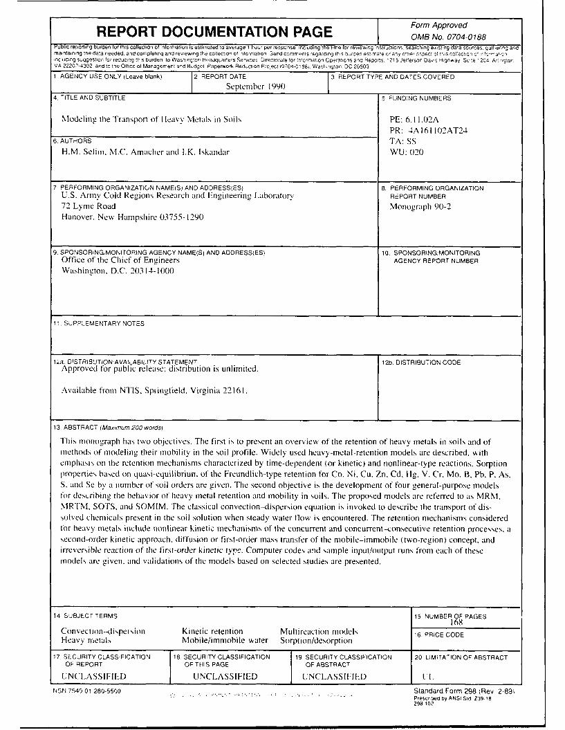
Form ApprovedREPORT DOCUMENTATION PAGE OMB No. 0704-0188Pubic reporting burden for this collection of information is estimated to average I hour per response including the fine for reviewng instructions. searching existing data sources gathering andmantaining the data needed, and completing and revewng the collection of intormatlon Send comments regarding rhs burden estimate or any other nspec o t;S co!,eci;or cf 5 %-f ""a, onincluding suggestion for reducing th s burden. to Washington Heaoquaiers Services Directorate for Information Opera:;uns and Reports. 1215 Jefferson Das HFghway Sc le 1204 Arr'gtonVA 22202-4302. and to the Office of Management and Budget Paperwork Reducton Project (0704-0188. Washington. DC 20503

1. AGENCY USE ONLY (Leave blank) 2. REPORT DATE REPORT TYPE AND DATES COVERED

I September 1990T

4, TITLE AND SUBTITLE 5. FUNDING NUMBERS

Modeling the Transport of Heavy Metals in Soils PE: 6.1 1.02APR: 4A161102AT24

6. AUTHORS TA: SSH.M. Selim. M.C. Amacher and I.K. Iskandar WU: 020

7. PERFORMING ORGANIZATICN NAME(S) AND ADDRESS(ES) 8. PERFORMING ORGANIZATION

U.S. Army Cold Regions Research and Engineering Laboratory REPORT NUMBER

72 Lyme Road Monograph 90-2Hanover. New Hampshire 03755-1290

9. SPONSORING-MONITORING AGENCY NAME(S) AND ADDRESS(ES) 10. SPONSORINGMONTORINGOffice of the Chief of Engineers AGENCY REPORT NUMBERWashington. D.C. 20314-1000

11. SUPPLEMENTARY NOTES

Ia. DISTRIBUTION AVAILABILITY STATEMENT 12b. DISTRIBUTION CODEApproved for public release; distribution is unlimited.

Available from NTIS. Springfield, Virginia 22161.

13. ABSTRACT (Maximum 200 words)

This monograph has two objectives. The first is to present an overview of the retention of heavy metals in soils and ofmethods of modeling their mobility in the soil profile. Widely used heavy-metal-retention models are described, withemphasis on the retention mechanisms characterized by time-dependent (or kinetic) and nonlinear-type reactions. Sorptionproperties based on quasi-equilibriun, of the Freundlich-type retention for Co, Ni, Cu, Zn, Cd. Hg, V. Cr, Mo, B, Pb, P. As,S. and Se by a number of soil orders are given. The second objective is the development of four general-purpose modelsfor describing the behavior of heavy metal retention and mobility in soils. The proposed models are referred to as MRNI,MRTM, SOTS. and SOMIM. Tile classical convection-dispersion equation is invoked to describe the transport of dis-solved chemicals present in the soil solution when steady water flow is encountered. The retention mechanisms consideredfor heavy metals include nonlinear kinetic mechanisms of the concurrent and concurrent-consecutive retention processes. asecond-order kinetic approach, diffusion or first-order mass transfer of the mobile-immobile (two-region) concept. andirreversible reaction of the first-order kinetic type. Computer codes and sample input/output runs from each of thesemodels are given. and validations of the models based on selected studies are presented.

14 SUBJECT TERMS 15. NUMBER OF PAGES168

Convection--dispersion Kinetic retention Multireaction models 16 PRICE CODEHeavy n-,etals Mobile/immobile water Sorption/desorption

17. SECURITY CLASSIFICATION 18. SECURITY CLASSIFICATION 19 SECURITY CLASSIFICATION 20 LIMITATION OF ABSTRACTOF REPORT OF THIS PAGE OF ABSTRACT

UNCLASSIFIED UNCLASSIFIED UNCLASSIFIED UlI.

NSN 7540 01 2805500 Standard Form 298 (Rev 2-891Prescribed by ANSI Std Z39.r8

298 102