modeling tail dependence using copulas — literature...
TRANSCRIPT
Modeling tail dependence using copulas — literature review
Jan de Kort
March 15, 2007
1
Contents
1 Bivariate Copulas 5
1.1 Sklar’s theorem . . . . . . . . . . . . . . . . . . . . . . . . . . . . . . . . . . . 7
1.2 Frechet-Hoeffding bounds . . . . . . . . . . . . . . . . . . . . . . . . . . . . . 9
1.3 Survival copula . . . . . . . . . . . . . . . . . . . . . . . . . . . . . . . . . . . 11
2 Multivariate Copulas 13
2.1 Sklar’s theorem . . . . . . . . . . . . . . . . . . . . . . . . . . . . . . . . . . . 14
2.2 Frechet-Hoeffding bounds . . . . . . . . . . . . . . . . . . . . . . . . . . . . . 14
3 Dependence 15
3.1 Linear correlation . . . . . . . . . . . . . . . . . . . . . . . . . . . . . . . . . . 15
3.2 Measures of concordance . . . . . . . . . . . . . . . . . . . . . . . . . . . . . . 16
3.2.1 Kendall’s tau . . . . . . . . . . . . . . . . . . . . . . . . . . . . . . . . 17
3.2.2 Spearman’s rho . . . . . . . . . . . . . . . . . . . . . . . . . . . . . . . 19
3.2.3 Gini’s gamma . . . . . . . . . . . . . . . . . . . . . . . . . . . . . . . . 20
3.3 Measures of dependence . . . . . . . . . . . . . . . . . . . . . . . . . . . . . . 21
3.3.1 Schweizer and Wolff’s sigma . . . . . . . . . . . . . . . . . . . . . . . . 21
3.4 Tail dependence . . . . . . . . . . . . . . . . . . . . . . . . . . . . . . . . . . . 22
3.5 Multivariate dependence . . . . . . . . . . . . . . . . . . . . . . . . . . . . . . 23
4 Parametric families of copulas 24
4.1 Frechet family . . . . . . . . . . . . . . . . . . . . . . . . . . . . . . . . . . . . 24
4.2 Elliptical distributions . . . . . . . . . . . . . . . . . . . . . . . . . . . . . . . 25
4.2.1 Bivariate Gaussian copula . . . . . . . . . . . . . . . . . . . . . . . . . 25
4.2.2 Bivariate Student’s t copula . . . . . . . . . . . . . . . . . . . . . . . . 26
4.3 Archimedean copulas . . . . . . . . . . . . . . . . . . . . . . . . . . . . . . . . 26
4.3.1 One-parameter families . . . . . . . . . . . . . . . . . . . . . . . . . . 26
4.3.2 Two-parameter families . . . . . . . . . . . . . . . . . . . . . . . . . . 27
4.3.3 Multivariate Archimedean copulas . . . . . . . . . . . . . . . . . . . . 28
4.4 Extension of Archimedean copulas . . . . . . . . . . . . . . . . . . . . . . . . 28
5 Calibration of Copulas from Market Data 30
5.1 Maximum likelihood method . . . . . . . . . . . . . . . . . . . . . . . . . . . 30
5.2 IFM method . . . . . . . . . . . . . . . . . . . . . . . . . . . . . . . . . . . . 31
5.3 CML method . . . . . . . . . . . . . . . . . . . . . . . . . . . . . . . . . . . . 31
2
6 Option Pricing with Copulas 32
6.1 Bivariate digital options . . . . . . . . . . . . . . . . . . . . . . . . . . . . . . 32
6.2 Rainbow options . . . . . . . . . . . . . . . . . . . . . . . . . . . . . . . . . . 33
7 Project plan 34
A Basics of derivatives pricing 35
A.1 No arbitrage and the market price of risk . . . . . . . . . . . . . . . . . . . . 35
A.2 Ito formula . . . . . . . . . . . . . . . . . . . . . . . . . . . . . . . . . . . . . 36
A.3 Fundamental PDE, Black-Scholes . . . . . . . . . . . . . . . . . . . . . . . . . 36
A.4 Martingale approach . . . . . . . . . . . . . . . . . . . . . . . . . . . . . . . . 37
B Implied quantities 41
B.1 Implied distribution . . . . . . . . . . . . . . . . . . . . . . . . . . . . . . . . 41
B.2 Implied volatility . . . . . . . . . . . . . . . . . . . . . . . . . . . . . . . . . . 42
3
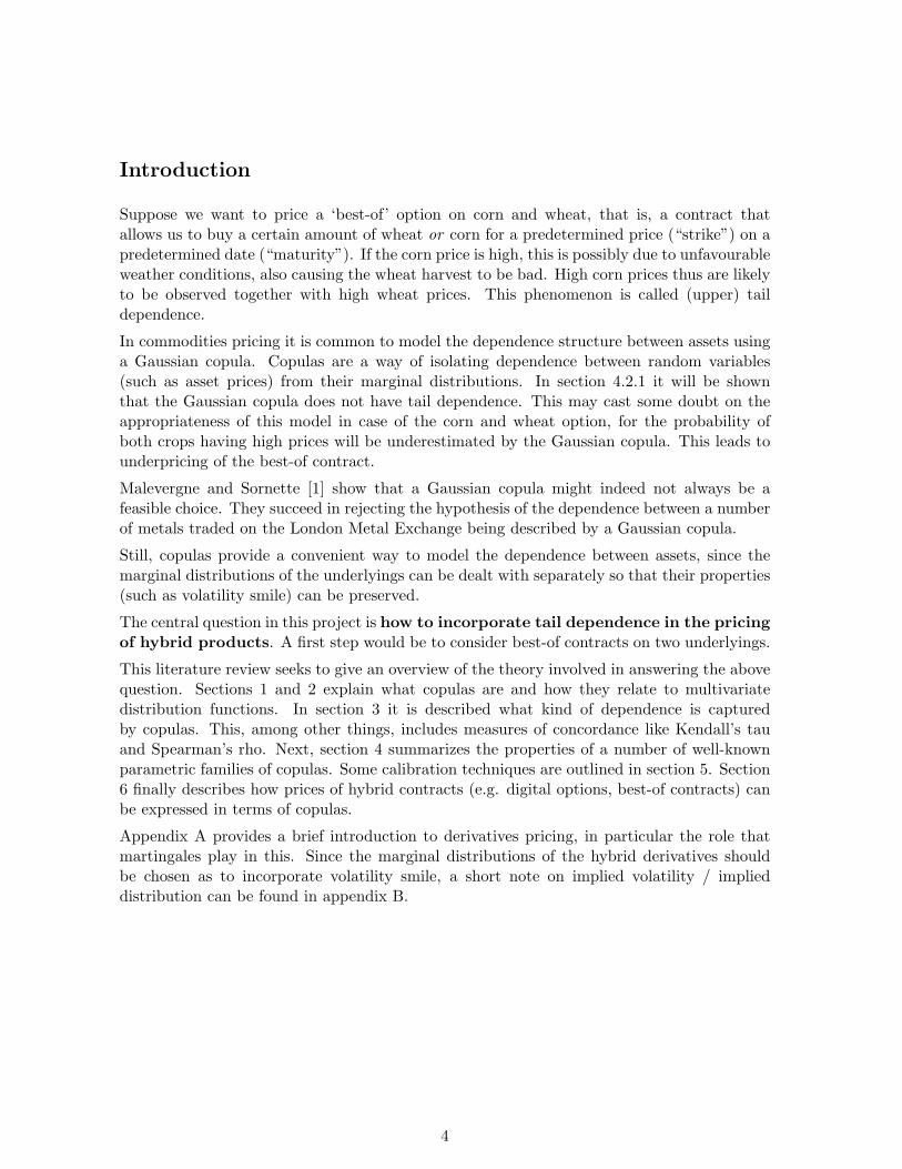
Introduction
Suppose we want to price a ‘best-of’ option on corn and wheat, that is, a contract thatallows us to buy a certain amount of wheat or corn for a predetermined price (“strike”) on apredetermined date (“maturity”). If the corn price is high, this is possibly due to unfavourableweather conditions, also causing the wheat harvest to be bad. High corn prices thus are likelyto be observed together with high wheat prices. This phenomenon is called (upper) taildependence.
In commodities pricing it is common to model the dependence structure between assets usinga Gaussian copula. Copulas are a way of isolating dependence between random variables(such as asset prices) from their marginal distributions. In section 4.2.1 it will be shownthat the Gaussian copula does not have tail dependence. This may cast some doubt on theappropriateness of this model in case of the corn and wheat option, for the probability ofboth crops having high prices will be underestimated by the Gaussian copula. This leads tounderpricing of the best-of contract.
Malevergne and Sornette [1] show that a Gaussian copula might indeed not always be afeasible choice. They succeed in rejecting the hypothesis of the dependence between a numberof metals traded on the London Metal Exchange being described by a Gaussian copula.
Still, copulas provide a convenient way to model the dependence between assets, since themarginal distributions of the underlyings can be dealt with separately so that their properties(such as volatility smile) can be preserved.
The central question in this project is how to incorporate tail dependence in the pricingof hybrid products. A first step would be to consider best-of contracts on two underlyings.
This literature review seeks to give an overview of the theory involved in answering the abovequestion. Sections 1 and 2 explain what copulas are and how they relate to multivariatedistribution functions. In section 3 it is described what kind of dependence is capturedby copulas. This, among other things, includes measures of concordance like Kendall’s tauand Spearman’s rho. Next, section 4 summarizes the properties of a number of well-knownparametric families of copulas. Some calibration techniques are outlined in section 5. Section6 finally describes how prices of hybrid contracts (e.g. digital options, best-of contracts) canbe expressed in terms of copulas.
Appendix A provides a brief introduction to derivatives pricing, in particular the role thatmartingales play in this. Since the marginal distributions of the hybrid derivatives shouldbe chosen as to incorporate volatility smile, a short note on implied volatility / implieddistribution can be found in appendix B.
4
1 Bivariate Copulas
This section introduces copulas and describes how they relate to multivariate distributions(i.e. Sklar’s theorem, section 1.1). Section 1.2 introduces the Frechet-Hoeffding upper andlower bounds for copulas. It is also explained what it means for a multivariate distribution ifits copula is maximal or minimal. Finally, in section 1.3, survival copulas are defined whichwill be useful in the discussion of tail dependence later on.
The extended real line R∪ −∞,+∞ is denoted by R.
Definition 1.1 Let ∅ 6= S1, S2 ⊂ R and let H be a S1 × S2 → R function. The H-volumeof B = [x1, x2]× [y1, y2] is defined to be
VH(B) = H(x2, y2)−H(x2, y1)−H(x1, y2) +H(x1, y1).
H is 2-increasing if VH(B) ≥ 0 for all B ⊂ S1 × S2.
Definition 1.2 Suppose b1 = maxS1 and b2 = maxS2 exist. Then the margins F and Gof H are given by
F : S1 → R, F (x) = H(x, b2),
G : S2 → R, G(y) = H(b1, y).
Note that b1 and b2 can possibly be +∞.
Definition 1.3 Suppose also a1 = minS1 and a2 = minS2 exist. H is called grounded if
H(a1, y) = H(x, a2) = 0
for all (x, y) ∈ S1 × S2.
Again, a1 and a2 can be −∞.
As H is 2-increasing we have, from definition 1.1,
H(x2, y2)−H(x1, y2) ≥ H(x2, y1)−H(x1, y1) (1)
andH(x2, y2)−H(x2, y1) ≥ H(x1, y2)−H(x1, y1) (2)
for every [x1, x2]× [y1, y2] ⊂ S1 × S2. By setting x1 = a1 in (1) and y1 = a2 in (2) it can beseen that
Lemma 1.4 Any grounded, 2-increasing function H : S1 × S2 → R is nondecreasing in botharguments, that is for all x1 ≤ x2 in S1 and y1 ≤ y2 in S2
H( · , y2) ≥ H( · , y1),H(x2, · ) ≥ H(x1, · ).
From lemma 1.4 it follows that (1) and (2) also hold in absolute value. Adding up theseinequalities and applying the triangle inequality (Figure 1) yields in particular
5

Figure 1: Schematic proof of lemma 1.5. Apply 2-increasingness to rectangle I and II andcombine the resulting inequalities via the triangle inequality. For the absolute value bars, usethat H is nondecreasing in both arguments (lemma 1.4).
Lemma 1.5 For any grounded, 2-decreasing function H : S1 × S2 → R,
|H(x2, y2)−H(x1, y1)| ≤ |F (x2)− F (x1)|+ |G(y2)−G(y1)|
for every [x1, x2]× [y1, y2] ⊂ S1 × S2.
Definition 1.6 A grounded, 2-increasing function C ′ : S1 × S2 → R where S1 and S2 aresubsets of [0, 1] containing 0 and 1, is called a (two dimensional) subcopula if for all (u, v) ∈S1 × S2
C ′(u, 1) = u,
C ′(1, v) = v.
Definition 1.7 A (two dimensional) copula is a subcopula whose domain is [0, 1]2.
Remark 1.8 Note that reformulating lemma 1.5 in terms of subcopulas immediately leads tothe Lipschitz condition
|C ′(u2, v2)− C ′(u1, v1)| ≤ |u2 − u1|+ |v2 − v1|, (u1, v1), (u2, v2) ∈ S1 × S2,
guarantying continuity of (sub)copulas.
Definition 1.9 The density associated with a copula C is
c(u, v) =∂2C(u, v)∂u∂v
.
6
Definition 1.10 The absolutely continuous component AC and the and the singularcomponent SC of the density are defined as
AC(u, v) =∫ u
0
∫ v
0
∂2C(s, t)∂u∂v
ds dt,
SC(u, v) = C(u, v)−AC(u, v).
1.1 Sklar’s theorem
The theorem under consideration in this section, due to Sklar in 1959, is the very reasonwhy copulas are popular for modeling purposes. It says that every joint distribution withcontinuous margins can be uniquely written as a copula function of its marginal distributions.This provides a way to seperate the study of joint distributions into the marginal distributionsand their joining copula.
Following Nelsen [2], we state Sklar’s theorem for subcopulas first, the proof of which is short.The corresponding result for copulas follows from a straightforward, but elaborate, extensionthat will be omitted.
Definition 1.11 Given a probability space (Ω,F ,P) — where Ω is the sample space, P ameasure such that P(Ω) = 1 and F ⊂ 2Ω a sigma-algebra — a random variable is definedto be a mapping
X : Ω → R
such that X is F-measurable.
Definition 1.12 Let X be a random variable. The cumulative distribution function(CDF) of X is
F : R→ [0, 1], F (x) := P[X ≤ x].
This will be denoted “X ∼ F”.
Definition 1.13 If the derivative of the CDF of X exists, it is called the probability densityfunction (pdf) of X.
Definition 1.14 Let X and Y be random variables. The joint distribution function ofX and Y is
H(x, y) := P[X ≤ x, Y ≤ y].
The margins of H are F (x) := limy→∞H(x, y) and G(y) := limx→∞H(x, y).
Definition 1.15 A random variable is said to be continuous if its CDF is continuous.
7
Lemma 1.16 Let H be a joint distribution function with margins F and G. Then thereexists a unique subcopula C ′ such that
DomC ′ = RanF × RanG
andH(x, y) = C ′(F (x), G(y)) (3)
for all (x, y) ∈ R.
Proof For C ′ to be unique, every (u, v) ∈ RanF ×RanG should have only one possible imageC ′(u, v) that is consistent with (3). Suppose to the contrary that C ′
1(u, v) 6= C ′2(u, v) are both
consistent with (3), i.e. there exist (x1, y1), (x2, y2) ∈ R2 such that
C ′1(u, v) = C ′
1(F (x1), G(y1)) = H(x1, y1),
C ′2(u, v) = C ′
2(F (x2), G(y2)) = H(x2, y2).
Thus, it must hold that u = F (x1) = F (x2) and v = G(y1) = G(y2). Being a joint CDF, Hsatisfies the requirements of lemma 1.5 and this yields
|H(x2, y2)−H(x1, y1)| ≤ |F (x2)− F (x1)|+ |G(y2)−G(y1)| = 0,
so C ′1 and C ′
2 agree on (u, v).
Now define C ′ to be the (unique) function mapping the pairs (F (x), G(y)) to H(x, y), for(x, y) ∈ R2. It remains to show that C ′ is a 2-subcopula.
Groundedness:C ′(0, G(y)) = C ′(F (−∞), G(y)) = H(−∞, y) = 0
C ′(F (x), 0) = C ′(F (x), G(−∞)) = H(x,−∞) = 0
2-increasingness:Let u1 ≤ u2 be in Ran F and v1 ≤ v2 in Ran G. As CDFs are nondecreasing, there existunique x1 ≤ x2, y1 ≤ y2 with F (x1) = u1, F (x2) = u2, G(y1) = v1 and G(y2) = v2.
C ′(u2, v2)− C ′(u1, v2)− C ′(u2, v1) + C ′(u1, v1)= C ′(F (x2), G(y2))− C ′(F (x1), G(y2))− C ′(F (x2), G(y1)) + C ′(F (x1), G(y1))= H(u2, v2)−H(u1, v2)−H(u2, v1) +H(u1, v1) ≥ 0
The last inequality follows from the sigma-additivity of P.
Margins are the identity mapping:
C ′(1, G(y)) = C ′(F (∞), G(y)) = H(∞, y) = G(y)
C ′(F (x), 1) = C ′(F (x), G(∞)) = H(x,∞) = F (x)
Remark 1.17 The converse of lemma 1.16 also holds: every H defined by (3) is a jointdistribution. This follows from the properties of a subcopula.
8
Theorem 1.18 (Sklar’s theorem) Let H be a joint distribution function with margins Fand G. Then there exists a unique 2-copula C such that for all (x, y) ∈ R2
H(x, y) = C(F (x), G(y)). (4)
If F and G are continuous then C is unique.
Conversely, if F and G are distribution functions and C is a copula, then H defined by (4)is a joint distribution function with margins F and G.
Proof Lemma 1.16 provides us with a unique subcopula C ′ satisfying (4). If F and G arecontinuous, then RanF ×RanG = I2 so C := C ′ is a copula. If not, it can be shown (see [2])that C ′ can be extended to a copula C.
The converse is a restatement of remark 1.17 for copulas.
Now that the connection between random variables and copulas is established via Sklar’stheorem, let us have a look at some implications.
Theorem 1.19 (C invariant under increasing transformation X and Y ) Let X ∼ Fand Y ∼ G be random variables with copula C. If α, β are increasing functions on RanXand RanY , then α(X) ∼ Fα and β(Y ) ∼ Gβ have copula Cαβ = C.
Proof
Cαβ(Fα(x), Gβ(y)) = P[α(X) ≤ x, β(Y ) ≤ y] = P[X < α−1(x), Y < β−1(y)]= C(F (α−1(x)), G(β−1(y))) = C(P[X < α−1(x)],P[Y < β−1(y)])= C(P[α(X) < x],P[β(Y ) < y]) = C(Fα(x), Gβ(y))
Let X ∼ F and Y ∼ G be continuous random variables with joint distribution H. X and Yare independent iff. H(x, y) = F (x)G(y). In terms of copulas this reads
Theorem 1.20 The continuous random variables X and Y are independent iff. their copulais C⊥(u, v) = uv.
C⊥ is called the product copula.
1.2 Frechet-Hoeffding bounds
In this section we will show the existence of a maximal and a minimal bivariate copula, usuallyrefered to as the Frechet-Hoeffing bounds. All other copulas take values in between thesebounds on each point of their domain, the unit square. The Frechet upper bound correspondsto perfect positive dependence and the lower bound to perfect negative dependence.
Theorem 1.21 For any subcopula C ′ with domain S1 × S2
C−(u, v) := max(u+ v − 1, 0) ≤ C ′(u, v) ≤ min(u, v) =: C+(u, v),
for every (u, v) ∈ S1 × S2. C+ and C− are called the Frechet-Hoeffding upper and lowerbounds respectively.
9
00.2
0.40.6
0.8
1 0
0.2
0.4
0.6
0.8
1
00.250.5
0.75
1
00.2
0.40.6
0.8
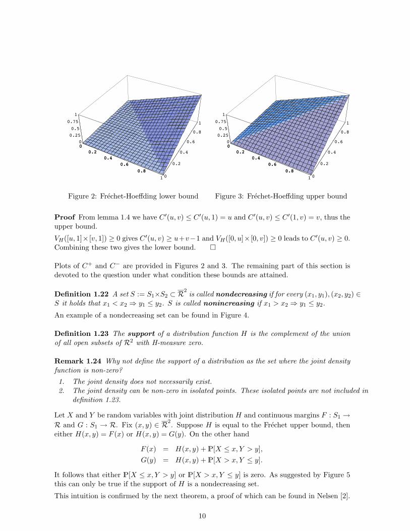
Figure 2: Frechet-Hoeffding lower bound
00.2
0.40.6
0.8
1 0
0.2
0.4
0.6
0.8
1
00.250.5
0.75
1
00.2
0.40.6
0.8
Figure 3: Frechet-Hoeffding upper bound
Proof From lemma 1.4 we have C ′(u, v) ≤ C ′(u, 1) = u and C ′(u, v) ≤ C ′(1, v) = v, thus theupper bound.
VH([u, 1]× [v, 1]) ≥ 0 gives C ′(u, v) ≥ u+v−1 and VH([0, u]× [0, v]) ≥ 0 leads to C ′(u, v) ≥ 0.Combining these two gives the lower bound.
Plots of C+ and C− are provided in Figures 2 and 3. The remaining part of this section isdevoted to the question under what condition these bounds are attained.
Definition 1.22 A set S := S1×S2 ⊂ R2 is called nondecreasing if for every (x1, y1), (x2, y2) ∈S it holds that x1 < x2 ⇒ y1 ≤ y2. S is called nonincreasing if x1 > x2 ⇒ y1 ≤ y2.
An example of a nondecreasing set can be found in Figure 4.
Definition 1.23 The support of a distribution function H is the complement of the unionof all open subsets of R2 with H-measure zero.
Remark 1.24 Why not define the support of a distribution as the set where the joint densityfunction is non-zero?
1. The joint density does not necessarily exist.2. The joint density can be non-zero in isolated points. These isolated points are not included in
definition 1.23.
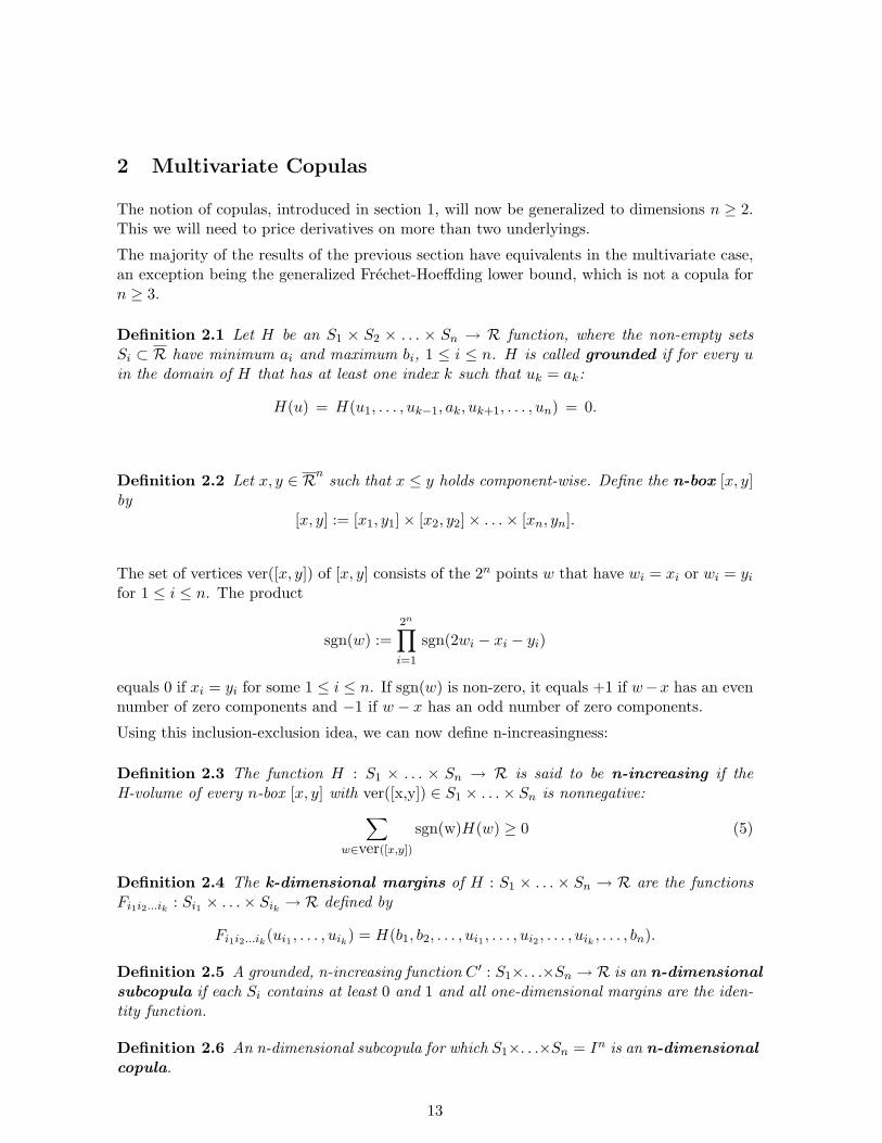
Let X and Y be random variables with joint distribution H and continuous margins F : S1 →R and G : S1 → R. Fix (x, y) ∈ R2. Suppose H is equal to the Frechet upper bound, theneither H(x, y) = F (x) or H(x, y) = G(y). On the other hand
F (x) = H(x, y) + P[X ≤ x, Y > y],G(y) = H(x, y) + P[X > x, Y ≤ y].
It follows that either P[X ≤ x, Y > y] or P[X > x, Y ≤ y] is zero. As suggested by Figure 5this can only be true if the support of H is a nondecreasing set.
This intuition is confirmed by the next theorem, a proof of which can be found in Nelsen [2].
10

Figure 4: Example of a nondecreasing set.
Theorem 1.25 Let X and Y be random variables with joint distribution function H.
H is equal to the upper Frechet-Hoeffding bound iff. the support of H is a nondecreasingsubset of R2.
H is equal to the lower Frechet-Hoeffding bound iff. the support of H is a nonincreasingsubset of R2.
Remark 1.26 If X and Y are continuous random variables, then the support of H cannothave horizontal or vertical segments. Indeed, suppose the support of H would have a horizontalline segment, then a relation of the form 0 < P[a ≤ X ≤ b] = P[Y = c] would hold, implyingthat the CDF of Y had a jump at c.
Thus, in case of continuous X and Y , theorem 1.25 implies the support of H to be an al-most surely increasing (decreasing) set iff. H is equal to the upper (lower) Frechet-Hoeffdingbound.
Remark 1.27 The support of H being an almost surely (in)(de)creasing set means that ifyou observe X, there is only one Y that can be observed simultaneously, and vice versa.Intuitively, this is exactly the notion of ‘perfect dependence’.
1.3 Survival copula
Every bivariate copula has a survival copula associated with it that gives the probability oftwo random variables both to exceed a certain value.
Definition 1.28 The survival copula associated with the copula C is
C(u, v) = u+ v − 1 + C(1− u, 1− v).
11
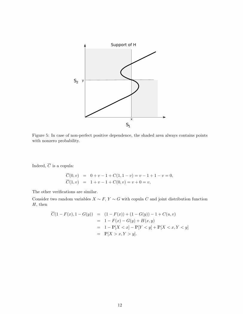
Figure 5: In case of non-perfect positive dependence, the shaded area always contains pointswith nonzero probability.
Indeed, C is a copula:
C(0, v) = 0 + v − 1 + C(1, 1− v) = v − 1 + 1− v = 0,C(1, v) = 1 + v − 1 + C(0, v) = v + 0 = v,
The other verifications are similar.
Consider two random variables X ∼ F, Y ∼ G with copula C and joint distribution functionH, then
C(1− F (x), 1−G(y)) = (1− F (x)) + (1−G(y))− 1 + C(u, v)= 1− F (x)−G(y) +H(x, y)= 1− P[X < x]− P[Y < y] + P[X < x, Y < y]= P[X > x, Y > y].
12
2 Multivariate Copulas
The notion of copulas, introduced in section 1, will now be generalized to dimensions n ≥ 2.This we will need to price derivatives on more than two underlyings.
The majority of the results of the previous section have equivalents in the multivariate case,an exception being the generalized Frechet-Hoeffding lower bound, which is not a copula forn ≥ 3.
Definition 2.1 Let H be an S1 × S2 × . . . × Sn → R function, where the non-empty setsSi ⊂ R have minimum ai and maximum bi, 1 ≤ i ≤ n. H is called grounded if for every uin the domain of H that has at least one index k such that uk = ak:
H(u) = H(u1, . . . , uk−1, ak, uk+1, . . . , un) = 0.
Definition 2.2 Let x, y ∈ Rn such that x ≤ y holds component-wise. Define the n-box [x, y]by
[x, y] := [x1, y1]× [x2, y2]× . . .× [xn, yn].
The set of vertices ver([x, y]) of [x, y] consists of the 2n points w that have wi = xi or wi = yifor 1 ≤ i ≤ n. The product
sgn(w) :=2n∏i=1
sgn(2wi − xi − yi)
equals 0 if xi = yi for some 1 ≤ i ≤ n. If sgn(w) is non-zero, it equals +1 if w−x has an evennumber of zero components and −1 if w − x has an odd number of zero components.
Using this inclusion-exclusion idea, we can now define n-increasingness:
Definition 2.3 The function H : S1 × . . . × Sn → R is said to be n-increasing if theH-volume of every n-box [x, y] with ver([x,y]) ∈ S1 × . . .× Sn is nonnegative:∑
w∈ver([x,y])sgn(w)H(w) ≥ 0 (5)
Definition 2.4 The k-dimensional margins of H : S1 × . . . × Sn → R are the functionsFi1i2...ik : Si1 × . . .× Sik → R defined by
Fi1i2...ik(ui1 , . . . , uik) = H(b1, b2, . . . , ui1 , . . . , ui2 , . . . , uik , . . . , bn).
Definition 2.5 A grounded, n-increasing function C ′ : S1×. . .×Sn → R is an n-dimensionalsubcopula if each Si contains at least 0 and 1 and all one-dimensional margins are the iden-tity function.
Definition 2.6 An n-dimensional subcopula for which S1×. . .×Sn = In is an n-dimensionalcopula.
13
2.1 Sklar’s theorem
Theorem 2.7 (Sklar’s theorem, multivariate case) Let H be an n-dimensional distri-bution function with margins F1, . . . , Fn. Then there exists an n-copula C such that for allu ∈ Rn
H(u1, . . . , un) = C(F (u1), . . . , F (un)). (6)
If F1, . . . , Fn are continuous, then C is unique.
Conversely, if F1, . . . , Fn are distribution functions and C is a copula, then H defined by (6).is a joint distribution function with margins F1, . . . , Fn.
2.2 Frechet-Hoeffding bounds
Theorem 2.8 For every copula C and any u ∈ In
C−(u) := max(u1 + u2 + . . .+ un − n+ 1, 0) ≤ C(u) ≤ min(u1, u2, . . . , un) := C+(u).
In the multidimensional case, the upper bound is still a copula, but the lower bound is not.
The following example, due to Schweizer and Sklar [3], shows that C− does not satisfy equation(5). Consider the n-box
[12 , 1]× . . .×
[12 , 1]. For 2-increasingness, in particular, the H-volume
of this n-box has to be nonnegative. This is not the case for n > 2:
max
1 + . . .+ 1− n+ 1, 0
︸ ︷︷ ︸=n−n+1=1
− n max
12
+ 1 + . . .+ 1− n+ 1, 0
︸ ︷︷ ︸= 1
2+(n−1)−n+1= 1
2
+(n
2
)max
12
+12
+ 1 + . . .+ 1− n+ 1, 0
︸ ︷︷ ︸=0
+ . . . . . . ± max
12
+ . . .+12− n+ 1, 0
︸ ︷︷ ︸
=0
= 1− n
2.
On the other hand, for every u ∈ In, n ≥ 3, there exists a copula C such that C(u) = C−(u)(see Nelsen [2]). This shows that a sharper lower bound does not exist.
14
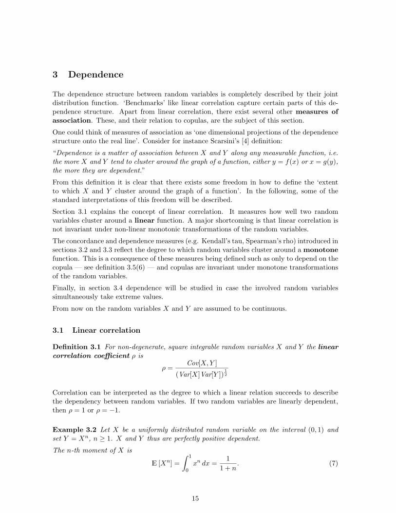
3 Dependence
The dependence structure between random variables is completely described by their jointdistribution function. ‘Benchmarks’ like linear correlation capture certain parts of this de-pendence structure. Apart from linear correlation, there exist several other measures ofassociation. These, and their relation to copulas, are the subject of this section.
One could think of measures of association as ‘one dimensional projections of the dependencestructure onto the real line’. Consider for instance Scarsini’s [4] definition:
“Dependence is a matter of association between X and Y along any measurable function, i.e.the more X and Y tend to cluster around the graph of a function, either y = f(x) or x = g(y),the more they are dependent.”
From this definition it is clear that there exists some freedom in how to define the ‘extentto which X and Y cluster around the graph of a function’. In the following, some of thestandard interpretations of this freedom will be described.
Section 3.1 explains the concept of linear correlation. It measures how well two randomvariables cluster around a linear function. A major shortcoming is that linear correlation isnot invariant under non-linear monotonic transformations of the random variables.
The concordance and dependence measures (e.g. Kendall’s tau, Spearman’s rho) introduced insections 3.2 and 3.3 reflect the degree to which random variables cluster around a monotonefunction. This is a consequence of these measures being defined such as only to depend on thecopula — see definition 3.5(6) — and copulas are invariant under monotone transformationsof the random variables.
Finally, in section 3.4 dependence will be studied in case the involved random variablessimultaneously take extreme values.
From now on the random variables X and Y are assumed to be continuous.
3.1 Linear correlation
Definition 3.1 For non-degenerate, square integrable random variables X and Y the linearcorrelation coefficient ρ is
ρ =Cov[X,Y ]
(Var[X]Var[Y ])12
Correlation can be interpreted as the degree to which a linear relation succeeds to describethe dependency between random variables. If two random variables are linearly dependent,then ρ = 1 or ρ = −1.
Example 3.2 Let X be a uniformly distributed random variable on the interval (0, 1) andset Y = Xn, n ≥ 1. X and Y thus are perfectly positive dependent.
The n-th moment of X is
E [Xn] =∫ 1
0xn dx =
11 + n
. (7)
15
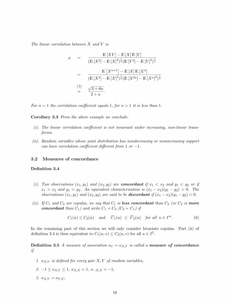
The linear correlation between X and Y is
ρ =E [XY ]− E [X]E [Y ]
(E [X2]− E [X]2)12 (E [Y 2]− E [Y ]2)
12
=E[Xn+1
]− E [X]E [Xn]
(E [X2]− E [X]2)12 (E [X2n]− E [Xn]2)
12
(7)=
√3 + 6n2 + n
.
For n = 1 the correlation coefficient equals 1, for n > 1 it is less than 1.
Corollary 3.3 From the above example we conclude:
(i). The linear correlation coefficient is not invariant under increasing, non-linear trans-forms.
(ii). Random variables whose joint distribution has nondecreasing or nonincreasing supportcan have correlation coefficient different from 1 or −1.
3.2 Measures of concordance
Definition 3.4
(i). Two observations (x1, y1) and (x2, y2) are concordant if x1 < x2 and y1 < y2 or ifx1 > x2 and y1 > y2. An equivalent characterisation is (x1 − x2)(y1 − y2) > 0. Theobservations (x1, y1) and (x2, y2) are said to be discordant if (x1 − x2)(y1 − y2) < 0.
(ii). If C1 and C2 are copulas, we say that C1 is less concordant than C2 (or C2 is moreconcordant than C1) and write C1 ≺ C2 (C2 C1) if
C1(u) ≤ C2(u) and C1(u) ≤ C2(u) for all u ∈ Im. (8)
In the remaining part of this section we will only consider bivariate copulas. Part (ii) ofdefinition 3.4 is then equivalent to C1(u, v) ≤ C2(u, v) for all u ∈ I2.
Definition 3.5 A measure of association κC = κX,Y is called a measure of concordanceif
1. κX,Y is defined for every pair X,Y of random variables,
2. −1 ≤ κX,Y ≤ 1, κX,X = 1, κ−X,X = −1,
3. κX,Y = κY,X ,
16

4. if X and Y are independent then κX,Y = κC⊥ = 0,
5. κ−X,Y = κX,−Y = −κX,Y ,
6. if C1 and C2 are copulas such that C1 ≺ C2 then κC1 ≤ κC2,
7. if (Xn, Yn) is a sequence of continuous random variables with copulas Cn and if Cnconverges pointwise to C, then limn→∞ κXn,Yn = κC .
What is the connection between definition 3.4 and 3.5?
By applying axiom (6) twice it follows that C1 = C2 implies κC1 = κC2 . If the randomvariablesX and Y have copula C and the transformations α and β are both strictly increasing,then CX,Y = Cα(X),β(Y ) by theorem 1.19 and consequently κX,Y = κα(X),β(Y ). Via axiom (5)a similar result for strictly decreasing transformations can be established. Measures ofconcordance thus are invariant under strictly monotone transformations of therandom variables.
If Y = α(X) and α is stictly increasing (decreasing), it follows from CX,α(X) = CX,X andaxiom (2) that κX,Y = 1 (−1). In other words: a measure of concordance assumes itsmaximal (minimal) value if the support of the joint distribution function of Xand Y contains only concordant (discordant) pairs. This explains how definitions 3.4and 3.5 are related.
Summarizing,
Lemma 3.6
(i). Measures of concordance are invariant under strictly monotone transformations of therandom variables.
(ii). A measure of concordance assumes its maximal (minimal) value if the support of thejoint distribution function of X and Y contains only concordant (discordant) pairs.
Note that these properties are exactly opposite to the conclusions in corollary 3.3 on the linearcorrelation coefficient. The linear correlation coefficient thus is not a measure of concordance.
In the remaining part of this section, two concordance measures will be described: Kendall’stau and Spearman’s rho.
3.2.1 Kendall’s tau
Let Q be the difference between the probability of concordance and discordance of two inde-pendent random vectors (X1, Y1) and (X2, Y2):
Q = P[(X1 −X2)(Y1 − Y2) > 0]− P[(X1 −X2)(Y1 − Y2) < 0].
In case (X1, Y1) and (X2, Y2) are iid. random vectors, the quantity Q is called Kendall’stau τ .
17
Given a sample (x1, y1), (x2, y2), . . . , (xn, yn) of n observations from a random vector (X,Y ),an unbiased estimator for τ is
t :=c− d
c+ d,
where c is the number of concordant pairs and d the number of discordant pairs in the sample.
Nelsen [2] shows that if (X1, Y1) and (X2, Y2) are independent random vectors with (possiblydifferent) distributions H1 and H2, but with common margins F , G and copulas C1, C2
Q = 4∫∫
I2C2(u, v) dC1(u, v)− 1. (9)
It follows that the probability of concordance between two bivariate distributions (with com-mon margins) minus the probability of discordance only depends on the copulas of each ofthe bivariate distributions.
Note that if C1 = C2 := C, then, since we already assumed common margins, the distributionsH1 and H2 are equal which means that (X1, Y1) and (X2, Y2) are identically distributed. Inthat case, (9) gives Kendall’s tau for the iid. random vectors (X1, Y1), (X2, Y2) with copula C.
Furthermore it can be shown that
τ = 1− 4∫∫
I2
∂C(u, v)∂u
∂C(u, v)∂v
du dv. (10)
In the particular case that C is absolutely continuous, the above relation can be deduced viaintegration by parts.
As an example of the use of (10), consider
Lemma 3.7 τC = τC .
Proof
τC = 1− 4∫∫
I2
∂C
∂u
∂C
∂vdu dv
= 1− 4∫∫
I2[1− ∂C
∂u][1− ∂C
∂v] du dv
= τC − 4∫∫
I2[1− ∂C
∂u− ∂C
∂v] du dv. (11)
The second term of the integrand of (11) reduces to∫∫I2
∂C
∂udu dv =
∫ 1
0C(1, v)− C(0, v) dv =
∫ 1
0C(1, v) dv =
∫ 1
0v dv =
12.
Similarly, ∫∫I2
∂C
∂vdu dv =
12.
Substituting in (11) yields the lemma.
Scarsini [4] proves axioms (1)–(7) of definition 3.5 hold for Kendall’s tau.
The next lemma does not hold for general concordance measures.
18
Lemma 3.8 Let H be a joint distribution with copula C.
C = C+ iff. τ = 1,C = C− iff. τ = −1.
Proof We will prove the first statement, C = C+ iff. τ = 1, via the following steps:
(i) τ = 1 ⇒ H has nondecreasing support(ii) H has nondecreasing support ⇒ H = C+
(iii) H = C+ ⇒ τ = 1
Step (ii) is immediate from theorem 1.25. Step (iii) follows from substitution of C+ in formula(9) and straightforward calculation. This step in fact also follows from axiom (6) in definition3.5.
It remains to show that τ = 1 implies H having nondecreasing support. Suppose thereforethat
1 = τ = P[(X1 −X2)(Y1 − Y2) > 0]− P[(X1 −X2)(Y1 − Y2) < 0].
Clearly,P[(X1 −X2)(Y1 − Y2) < 0] = 0. (12)
Now suppose that (x1, y1) and (x2, y2) are disconcordant and lie in the support of H. Inte-grating (12) over I2 yields
0 =∫∫
I2P[(X1 −X2)(Y1 − Y2) < 0] du dv
=∫∫
I2P[(X2 − x1)(Y2 − y1) < 0|(X1, Y1) = (x1, y1)] dH(u, v)
=∫∫
I2
P[X2 > x1, Y2 < y1|(X1, Y1) = (x1, y1)] + P[X2 < x1, Y2 > y1|(X1, Y1) = (x1, y1)]
dH(u, v).
It follows that there is no probability mass in the regions (u, v) : u > x1, v < y1 and(u, v) : u < x1, v > y1. In particular
P[Br(x1, y1)] = 0,
where r := 12 |minx1 − x2, y1 − y2| and Br(x, y) denotes an open 2-ball with radius r and
centre (x, y). Apparently (x1, y1) is not in the complement of the union of open sets havingzero probability and therefore not in the support of H. This contradicts our assumption andproves (i).
3.2.2 Spearman’s rho
Let (X1, Y1), (X2, Y2) and (X3, Y3) be iid. random vectors with common joint distribution H,margins F , G and copula C. Spearman’s rho is defined to be proportional to the probabilityof concordance minus the probability of discordance of the pairs (X1, Y1︸ ︷︷ ︸
Joint distr. H
) and (X2, Y3︸ ︷︷ ︸Independent
):
ρS = 3 ( P[(X1 −X2)(Y1 − Y3) > 0]− P[(X1 −X2)(Y1 − Y3) < 0] ).
19
Note thatX2 and Y3, being independent, have copula C⊥. By (9), three times the concordancedifference between C and C⊥ is
ρS = 3(
4∫∫
I2C(u, v)dC⊥(u, v)− 1
)= 12
∫∫I2C(u, v) du dv − 3. (13)
Spearman’s rho satisfies the axioms in definition 3.5 (see Nelsen [2]).
Let X ∼ F and Y ∼ G be random variables with copula C, then Spearman’s rho is equiv-alent to the linear correlation between F (X) and G(Y ). To see this, recall from prob-ability theory that F (X) and G(Y ) are uniformly distributed on the interval (0, 1), soE [F (X)] = E [G(Y )] = 1/2 and Var[F (X)] = Var[G(Y )] = 1/12. We thus have
ρS
(13)= 12E [F (X), G(Y )]− 3
=E [F (X), G(Y )]− (1/2)2
1/12
=E [F (X), G(Y )]− E [F (X)]E [G(Y )]
(Var[F (X)]Var[G(Y )])12
=Cov[F (X), G(Y )]
(Var[F (X)]Var[G(Y )])12
.
Cherubini et al. [5] states that for Spearman’s rho a statement similar to lemma 3.8 holds:C = C± iff. ρS = ±1.
3.2.3 Gini’s gamma
Whereas Spearman’s rho measures the concordance difference between a copula C and inde-pendence, Gini’s gamma γC measures the concordance difference between a copula C andmonotone dependence, i.e. the copulas C+ and C−. Using (9) this reads
γC =∫∫
I2C(u, v)dC−(u, v) +
∫∫I2C(u, v)dC+(u, v)
= 4[∫ 1
0C(u, 1− u)du−
∫ 1
0
(u− C(u, u)
)du
].
Gini’s gamma thus can be interpreted as the area between the secondary diagonal sections ofC and C−, minus the area between the diagonal sections of C+ and C.
20
3.3 Measures of dependence
Definition 3.9 A measure of association δC = δX,Y is called a measure of dependence if
1. δX,Y is defined for every pair X,Y of random variables,
2. 0 ≤ δX,Y ≤ 1
3. δX,Y = δY,X ,
4. δX,Y = 0 iff. X and Y are independent,
5. δX,Y = 1 iff. X and Y are strictly monotone functions of eachother,
6. if α and β are strictly monotone functions on Ran X and Ran Y respectively, thenδX,Y = δα(X),β(Y ),
7. if (Xn, Yn) is a sequence of continuous random variables with copulas Cn and if Cnconverges pointwise to C, then limn→∞ δXn,Yn = δC .
The differences between dependence and concordance measures are:
(i). Concordance measures assume their maximal (minimal) values if the concerning randomvariables are perfectly positive (negative) dependent. Dependence measures assumetheir extreme values if and only if the random variables are perfectly dependent.
(ii). Concordance measures are zero in case of independence. Dependence measures are zeroif and only if the random variables under consideration are independent.
(iii). The stronger properties of dependence measures over concordance measures go at thecost of a sign, or, in the words of Scarsini [4]:“[..] dependence is a matter of assocation with respect to a (strictly) monotone function(indifferently increasing or decreasing). [..] Concordance, on the other hand, takes intoaccount the kind of monotonicity [..] the maximum is attained when a strictly increasingrelation exists [..] the minimum [..] when a relation exists that is strictly monotonedecreasing.”
3.3.1 Schweizer and Wolff’s sigma
Schweizer and Wolff’s sigma σ for two random variables with copula C is given by
σC = 12∫∫
I2|C(u, v)− uv| dudv.
Nelsen [2] shows this association measure to satisfy the properties of definition 3.9.
21
3.4 Tail dependence
This section examines dependence in the upper-right and lower-left quadrant of I2.
Definition 3.10 Given two random variables X ∼ F and Y ∼ G with copula C, define thecoefficients of tail dependency
λL := limu↓0
P[F (X) < u|G(Y ) < u] = limu↓0
C(u, u)u
, (14)
λU := limu↑1
P[F (X) > u|G(Y ) > u] = limu↑1
1− 2u+ C(u, u)1− u
. (15)
C is said to have lower (upper) tail dependence iff. λL 6= 0 (λU 6= 0).
The interpretation of the coefficients of tail dependency is that it measures the probability oftwo random variables both taking extreme values.
Lemma 3.11 Denote the lower (upper) coefficient of tail dependency of the survival copulaC by λL (λU ), then
λL = λU ,
λU = λL.
Proof
λL = limu↓0
C(u, u)u
= limv↑1
C(1− v, 1− v)1− v
= limv↑1
1− 2v + C(v, v)1− v
= λU
λU = limu↑1
1− 2u+ C(u, u)1− u
= limu↓0
2v − 1 + C(1− v, 1− v)v
= limu↓0
C(v, v)v
= λL
Example 3.12 As an example, consider the Gumbel copula
CGumbel(u, v) := exp−[(− log u)1α + (− log v)
1α ]α, α ∈ [1,∞)
with diagonal section
CGumbel(u) := CGumbel(u, u) = u2α.
C is differentiable in both (0, 0) and (1, 1), this is a sufficient condition for the limits (14)and (15) to exist:
λL =dC
du(0)
=[d
duu2α
]u=0
=[2αu2α−1
]u=0
= 0 ,
λU = λL =d
du
[2u− 1 + C(1− u)
]u=0
= 2− dC
du(1)
= 2−[d
duu2α
]u=1
= 2− [ 2αu2α−1 ]u=1 = 2− 2α.
So the Gumbel copula has no lower tail dependency. It has upper tail dependency iff. α 6= 1.
22
3.5 Multivariate dependence
Most of the concordance and dependence measures introduced in the previous sections haveone or more multivariate generalizations.
Joe [6] obtains the following generalized version of Kendall’s tau. Let X = (X1, . . . , Xm) andY = (Y1, . . . , Ym) be iid. random vectors with copula C and define Dj := Xj − Yj . Denoteby Bk,m−k the set of m-tuples in Rm with k positive and m − k negative components. Ageneralized version of Kendall’s tau is given by
τC =m∑
k=bm+12
c
wk P( (D1, . . . , Dm) ∈ Bk,m−k)
where the weights wk, bm+12 c ≤ k ≤ m, are such that
(i). τC = 1 if C = C+,
(ii). τC = 0 if C = C⊥,
(iii). τC1 < τC2 whenever C1 ≺ C2.
The implications of (i) and (ii) for the wk’s are straightforward:
(i). wm = 1,
(ii).∑m
k=0wk(mk
)= 0 (wk := wm−k for k < bm+1
2 c).
The implication of (iii) is more involved (see [6], p. 18), though it is clear that at leastwm ≥ wm−1 ≥ . . . ≥ wbm+1
2c should hold.
For m = 3 the only weights satisfying (i)–(iii) are w3 = 1 and w2 = −13 . The minimal value
of τ for m = 3 thus is −13 . For m = 4 there exists a one-dimensional family of generalizations
of Kendall’s tau.
In terms of copulas, Joe’s generalization of Spearman’s rho ([6], pp. 22–24) for am-multivariatedistribution function having copula C reads
ωC =(∫
. . .
∫Im
C(u) du1 . . . dum − 2−m)/(
(m+ 1)−1 + 2−m).
Properties (i) and (ii) are taken care of by the scaling and normalization constants and can bechecked by substituting C+ and C⊥. The increasingness of ω with respect to ≺ is immediatefrom definition 3.4(ii).
There also exist multivariate measures of dependence. For instance, Nelsen [2] mentions thefollowing generalization of Schweizer and Wolff’s sigma:
σC =2m(m+ 1)
2m − (m+ 1)
∫. . .
∫Im
|C(u1, . . . , um)− u1 . . . um| du1 . . . dum,
where C is an m-copula.
23
4 Parametric families of copulas
This section gives an overview of some types of parametric families of copulas. We areparticularly interested in their coefficients of tail dependence.
The Frechet family (section 4.1) arises by taking affine linear combinations of the productcopula and the Frechet-Hoeffding upper and lower bounds. Tail dependence is determined bythe weights in the linear combination.
In section 4.2 copulas are introduced which stem from elliptical distributions. Because oftheir symmetric nature, upper and lower tail dependence coefficients are equal.
Any function satisfying certain properties (described in section 4.3) generates an Archimedeancopula. These copulas can take a great variety of forms. Furthermore, they can have dis-tinct upper and lower tail dependence coefficients. This makes them suitable candidates formodeling asset prices, since in market data either upper or lower tail dependence tends to bemore profound.
Multivariate Archimedean copulas however are of limited use in practice as all bivariatemargins are equal. Therefore in section 4.4 an extension of the class of Archimedean copulaswill be discussed that allows for several distinct bivariate margins.
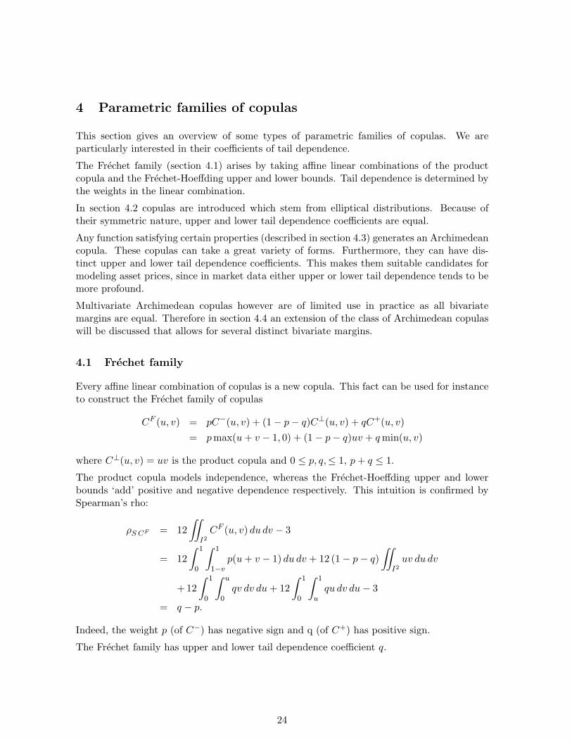
4.1 Frechet family
Every affine linear combination of copulas is a new copula. This fact can be used for instanceto construct the Frechet family of copulas
CF (u, v) = pC−(u, v) + (1− p− q)C⊥(u, v) + qC+(u, v)= pmax(u+ v − 1, 0) + (1− p− q)uv + qmin(u, v)
where C⊥(u, v) = uv is the product copula and 0 ≤ p, q,≤ 1, p+ q ≤ 1.
The product copula models independence, whereas the Frechet-Hoeffding upper and lowerbounds ‘add’ positive and negative dependence respectively. This intuition is confirmed bySpearman’s rho:
ρS CF = 12∫∫
I2CF (u, v) du dv − 3
= 12∫ 1
0
∫ 1
1−vp(u+ v − 1) du dv + 12 (1− p− q)
∫∫I2uv du dv
+12∫ 1
0
∫ u
0qv dv du+ 12
∫ 1
0
∫ 1
uqu dv du− 3
= q − p.
Indeed, the weight p (of C−) has negative sign and q (of C+) has positive sign.
The Frechet family has upper and lower tail dependence coefficient q.
24
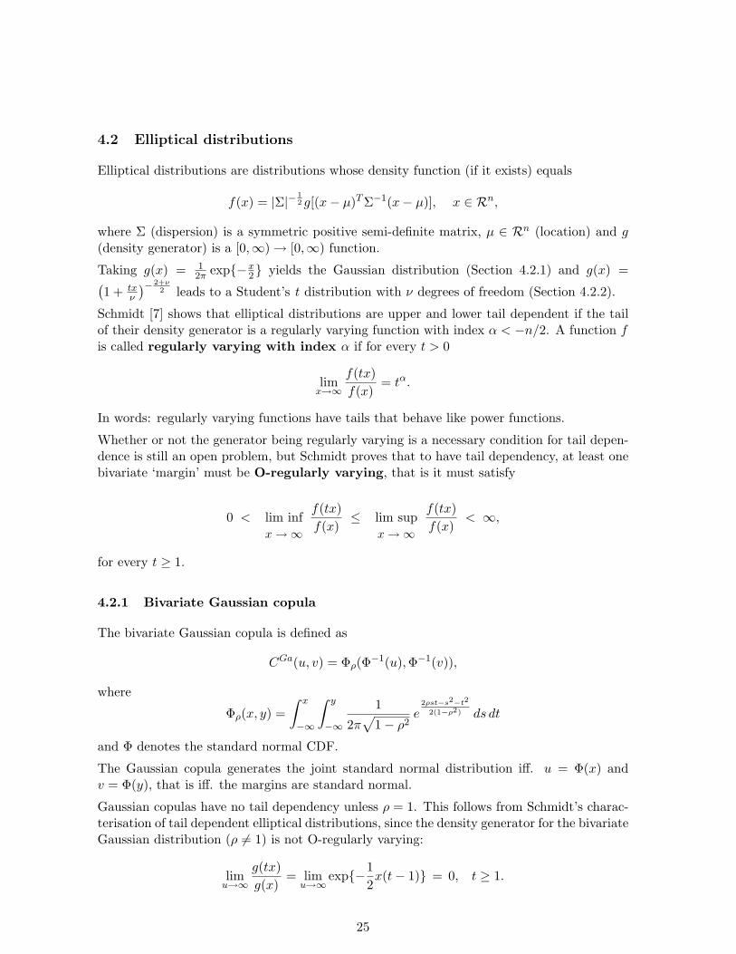
4.2 Elliptical distributions
Elliptical distributions are distributions whose density function (if it exists) equals
f(x) = |Σ|−12 g[(x− µ)TΣ−1(x− µ)], x ∈ Rn,
where Σ (dispersion) is a symmetric positive semi-definite matrix, µ ∈ Rn (location) and g(density generator) is a [0,∞) → [0,∞) function.
Taking g(x) = 12π exp−x
2 yields the Gaussian distribution (Section 4.2.1) and g(x) =(1 + tx
ν
)− 2+ν2 leads to a Student’s t distribution with ν degrees of freedom (Section 4.2.2).
Schmidt [7] shows that elliptical distributions are upper and lower tail dependent if the tailof their density generator is a regularly varying function with index α < −n/2. A function fis called regularly varying with index α if for every t > 0
limx→∞
f(tx)f(x)
= tα.
In words: regularly varying functions have tails that behave like power functions.
Whether or not the generator being regularly varying is a necessary condition for tail depen-dence is still an open problem, but Schmidt proves that to have tail dependency, at least onebivariate ‘margin’ must be O-regularly varying, that is it must satisfy
0 < lim infx→∞
f(tx)f(x)
≤ lim supx→∞
f(tx)f(x)
< ∞,
for every t ≥ 1.
4.2.1 Bivariate Gaussian copula
The bivariate Gaussian copula is defined as
CGa(u, v) = Φρ(Φ−1(u),Φ−1(v)),
where
Φρ(x, y) =∫ x
−∞
∫ y
−∞
1
2π√
1− ρ2e
2ρst−s2−t2
2(1−ρ2) ds dt
and Φ denotes the standard normal CDF.
The Gaussian copula generates the joint standard normal distribution iff. u = Φ(x) andv = Φ(y), that is iff. the margins are standard normal.
Gaussian copulas have no tail dependency unless ρ = 1. This follows from Schmidt’s charac-terisation of tail dependent elliptical distributions, since the density generator for the bivariateGaussian distribution (ρ 6= 1) is not O-regularly varying:
limu→∞
g(tx)g(x)
= limu→∞
exp−12x(t− 1) = 0, t ≥ 1.
25
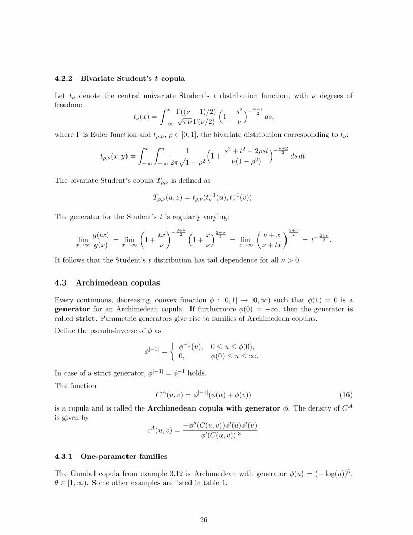
4.2.2 Bivariate Student’s t copula
Let tν denote the central univariate Student’s t distribution function, with ν degrees offreedom:
tν(x) =∫ x
−∞
Γ((ν + 1)/2)√πν Γ(ν/2)
(1 +
s2
ν
)− ν+12ds,
where Γ is Euler function and tρ,ν , ρ ∈ [0, 1], the bivariate distribution corresponding to tν :
tρ,ν(x, y) =∫ x
−∞
∫ y
−∞
1
2π√
1− ρ2
(1 +
s2 + t2 − 2ρstν(1− ρ2)
)− ν+22ds dt.
The bivariate Student’s copula Tρ,ν is defined as
Tρ,ν(u, z) = tρ,ν(t−1ν (u), t−1
ν (v)).
The generator for the Student’s t is regularly varying:
limx→∞
g(tx)g(x)
= limx→∞
(1 +
tx
ν
)− 2+ν2 (
1 +x
ν
) 2+ν2 = lim
x→∞
(ν + x
ν + tx
) 2+ν2
= t−2+ν2 .
It follows that the Student’s t distribution has tail dependence for all ν > 0.
4.3 Archimedean copulas
Every continuous, decreasing, convex function φ : [0, 1] → [0,∞) such that φ(1) = 0 is agenerator for an Archimedean copula. If furthermore φ(0) = +∞, then the generator iscalled strict. Parametric generators give rise to families of Archimedean copulas.
Define the pseudo-inverse of φ as
φ[−1] =φ−1(u), 0 ≤ u ≤ φ(0),0, φ(0) ≤ u ≤ ∞.
In case of a strict generator, φ[−1] = φ−1 holds.
The functionCA(u, v) = φ[−1](φ(u) + φ(v)) (16)
is a copula and is called the Archimedean copula with generator φ. The density of CA
is given by
cA(u, v) =−φ′′(C(u, v))φ′(u)φ′(v)
[φ′(C(u, v))]3.
4.3.1 One-parameter families
The Gumbel copula from example 3.12 is Archimedean with generator φ(u) = (− log(u))θ,θ ∈ [1,∞). Some other examples are listed in table 1.
26
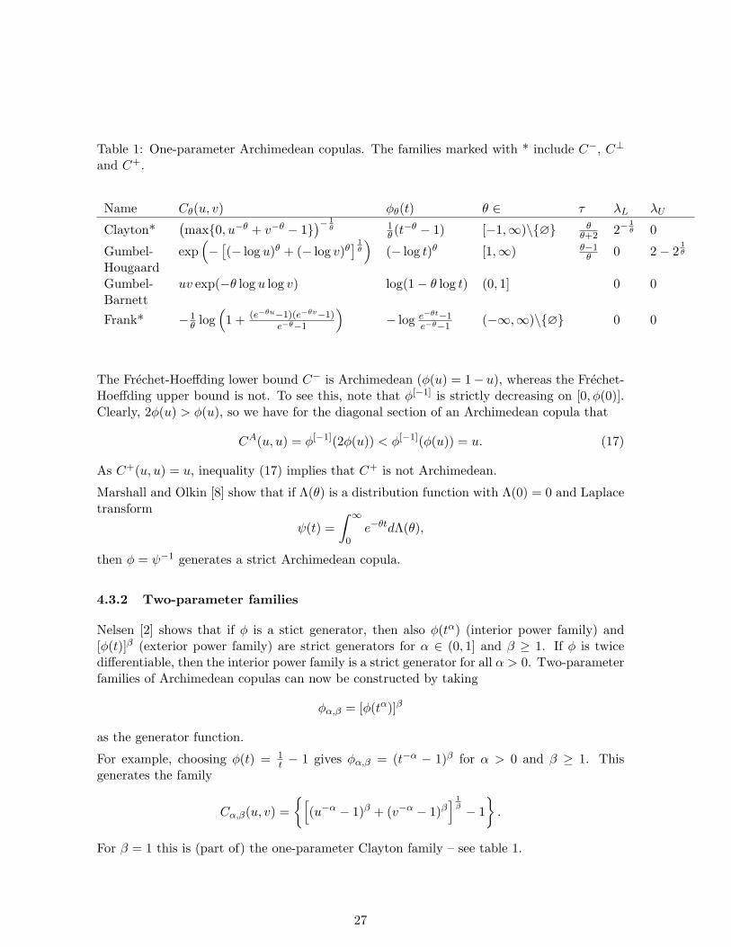
Table 1: One-parameter Archimedean copulas. The families marked with * include C−, C⊥
and C+.
Name Cθ(u, v) φθ(t) θ ∈ τ λL λU
Clayton*(max0, u−θ + v−θ − 1
)− 1θ 1
θ (t−θ − 1) [−1,∞)\∅ θ
θ+2 2−1θ 0
Gumbel-Hougaard
exp(−[(− log u)θ + (− log v)θ
] 1θ
)(− log t)θ [1,∞) θ−1
θ 0 2− 21θ
Gumbel-Barnett
uv exp(−θ log u log v) log(1− θ log t) (0, 1] 0 0
Frank* −1θ log
(1 + (e−θu−1)(e−θv−1)
e−θ−1
)− log e−θt−1
e−θ−1(−∞,∞)\∅ 0 0
The Frechet-Hoeffding lower bound C− is Archimedean (φ(u) = 1− u), whereas the Frechet-Hoeffding upper bound is not. To see this, note that φ[−1] is strictly decreasing on [0, φ(0)].Clearly, 2φ(u) > φ(u), so we have for the diagonal section of an Archimedean copula that
CA(u, u) = φ[−1](2φ(u)) < φ[−1](φ(u)) = u. (17)
As C+(u, u) = u, inequality (17) implies that C+ is not Archimedean.
Marshall and Olkin [8] show that if Λ(θ) is a distribution function with Λ(0) = 0 and Laplacetransform
ψ(t) =∫ ∞
0e−θtdΛ(θ),
then φ = ψ−1 generates a strict Archimedean copula.
4.3.2 Two-parameter families
Nelsen [2] shows that if φ is a stict generator, then also φ(tα) (interior power family) and[φ(t)]β (exterior power family) are strict generators for α ∈ (0, 1] and β ≥ 1. If φ is twicedifferentiable, then the interior power family is a strict generator for all α > 0. Two-parameterfamilies of Archimedean copulas can now be constructed by taking
φα,β = [φ(tα)]β
as the generator function.
For example, choosing φ(t) = 1t − 1 gives φα,β = (t−α − 1)β for α > 0 and β ≥ 1. This
generates the family
Cα,β(u, v) =[
(u−α − 1)β + (v−α − 1)β] 1
β − 1.
For β = 1 this is (part of) the one-parameter Clayton family – see table 1.
27
4.3.3 Multivariate Archimedean copulas
This section extends the notion of an Archimedean copula to dimensions n ≥ 2.
Kimberling [9] proves that if φ is a strict generator satisfying
(−1)kdkφ−1(t)dtk
≥ 0 for all t ∈ [0,∞), k = 1, . . . , n (18)
thenCA(u1, . . . , un) = φ−1(φ(u1) + . . .+ φ(un))
is an n-copula.
For example, the generator φθ(t) = t−θ−1 (θ > 0) of the bivariate Clayton family has inverseφ−1θ (t) = (1 + t)−
1θ which is readily seen to satisfy (18). Thus,
Cθ(u1, . . . , un) =(u−θ1 + . . .+ u−θn − n+ 1
)− 1θ
is a family of n-copulas.
It can be proven (see [10]) that Laplace transforms of distribution functions Λ(θ) satisfy (18)and Λ(0) = 1. The inverses of these transforms thus are a source of Archimedean n-copulas.
Archimedean n-copulas have practical restraints. To begin with, all k-margins are identical.Also, since there are usually only two parameters, Archimedean n-copulas are not very flexibleto fit the n dimensional dependence structure. Furthermore, Archimedean copulas that havegenerators with complete monotonic inverse, are always more concordant than the productcopula, i.e. they always model positive dependence.
There exist extensions of Archimedean copulas that have a number of mutually distinctbivariate margins. This is discussed in the next section.
4.4 Extension of Archimedean copulas
Generators of Archimedean copulas can be used to construct other (non-Archimedean) cop-ulas. One such extension is discussed in Joe [11]. Copulas that are constructed in this wayhave the property of partial exchangeability, i.e. a number of bivariate margins are mutu-ally distinct. We will only address the three dimensional case, but generalizations to higherdimensions are similar.
First, let φ be a strict generator and note that Archimedean copulas are associative:
C(u, v, w) = φ−1(φ(u) + φ(v) + φ(w))= φ−1(φ φ−1(φ(u) + φ(v))︸ ︷︷ ︸
C(u,v)
+φ(w))
= C(C(u, v), w).
If we would choose the generator of the ‘inner’ and the ‘outer’ copula to be different, wouldthe composition then still be a copula? In other words, for which functions φ, ψ is
Cφ(Cψ(u, v), w) (19)
28

a copula? If it is, then the (1,2) bivariate margin is different from the (1,3) margin, but the(2,3) margin is equal to the (1,3) margin.
For n = 1, 2, . . . ,∞, consider the following function classes:
Ln =φ : [0, φ) → [0, 1]
∣∣∣φ(0) = 1, φ(∞) = 0, (−1)kdkφ(t)dtk
≥ 0 for all t ∈ [0,∞), k = 1, . . . , n,
L∗n =ω : [0,∞) → [0,∞)
∣∣∣ω(0) = 0, ω(∞) = ∞, (−1)k−1dkω(t)dtk
≥ 0 for all t ∈ [0,∞), k = 1, . . . , n,
Note that if φ−1 ∈ L1, then φ is a strict generator for an Archimedean copula.
It turns out that if φ, ψ ∈ L1 and φ ψ−1 ∈ L∗∞, then (19) is a copula. For general n-copulassimilar conditions exist. In the n-dimensional case, n− 1 of the 1
2n(n− 1) bivariate marginsare distinct.
29
5 Calibration of Copulas from Market Data
This section is concerned with the question which member of a parametric family of copulasfits best to a given set of market data.
Consider a stochastic process Yt, t = 1, 2, . . . taking values in Rn. Our data consists in arealisation (x1t, . . . , xnt) : t = 1, . . . , T of the vectors Yt, t = 1, . . . , T.
5.1 Maximum likelihood method
Let Xi ∼ Fi, 1 ≤ i ≤ n, be random variables with joint distribution H. From the multidi-mensional version of Sklar’s theorem we know there exists a copula C such that
H(u1, . . . , un) = C(F (u1), . . . , F (un)).
Differentiating this expression to u1, u2, . . . , un sequentially yields the canonical represen-tation
h(u1, . . . , un) = c(F1(u1), . . . , Fn(un))n∏i=1
fi(ui), (20)
where c is the copula density.
The maximum likelihood method implies choosing C and F1, . . . , Fn such that the probabilityof observing the data set is maximal. The possible choices for the copula and the marginsare unlimited, or, in the words of Cherubini et al. [5], “copulas allow a double infinity ofdegrees of freedom”. Therefore we usually restrict ourselves to certain classes of functions,parametrized by some vector θ ∈ Θ ⊂ Rn.
We should thus find θ ∈ Θ that maximizes the likelihood
l(θ) :=T∏t=1
(c(F1(x1t), . . . , Fn(xnt); θ)
n∏i=1
fi(xit; θ)
).
This θ also maximimes the log-likelihood
log l(θ) =T∑t=1
log c(F1(x1t), . . . , Fn(xnt); θ) +T∑t=1
n∑i=1
log fi(xit; θ). (21)
The latter expression is often computationally more convenient. The vector θ that maximizesl(θ) is called the maximum likelihood estimator (MLE):
θMLE := argmaxθ ∈ Θ
l(θ).
If ∂l(θ)/∂θ exists, then the solutions of
∂l(θ)∂θ
= 0
30
are possible candidates for θMLE. But these solutions can also be local maxima, minimaor inflection points. On the other hand, maxima can occur at the boundary of Θ (or if||θ|| → ∞), in discontinuity points and in points where the likelihood is not differentiable.
For joint distributions satisfying some regularity conditions, it can be shown (Shao [12]) thatif the sample size increases, the subsequent MLEs converge to a limit. This property is calledconsistency.
5.2 IFM method
The log-likelihood (21) consists of two positive parts. Joe and Xu [13] proposed the setof parameters θ to be estimated in two steps: first the margins’ parameters and then thecopulas’. By doing so, the computational cost of finding the optimal set of parameters reducessignificantly. This approach is called the Inference for the Margins (IFM) method.
θ1 = argmaxθ2
T∑t=1
n∑i=1
log fi(xit; θ1)
θ2 = argmaxθ1
T∑t=1
log c(F1(x1t), . . . , Fn(xnt); θ1, θ2)
Set θIFM := (θ1, θ2) to be the IFM estimator. In general, this estimator will be different fromthe MLE, but it can be shown that the IFM estimator is consistent.
5.3 CML method
In the Canonical Maximum Likelihood (CML) method first the margins are estimated usingempirical distributions F1, . . . , Fn. Then, the copula parameters are estimated using an MLapproach:
θCML := argmaxθ
T∑t=1
log c(F1(x1t), . . . , Fn(xnt); θ).
31
6 Option Pricing with Copulas
In this section, existing pricing techniques for (bivariate) digital and rainbow options withdependent underlyings will be restated in terms of copulas. Following Cherubini et al. [5], amartingale approach will be used. An outline of martingale pricing is given in appendix A.4.
We will need a reformulation of Sklar’s theorem in terms of conditional copulas. Conditionalcopulas are defined along the same lines as in section 1, details can be found in Patton [14].
Theorem 6.1 (Sklar’s theorem for conditional copulas) Let X|Ft ∼ F (·|Ft), Y |Ft ∼G(·|Ft) be random variables with joint conditional distribution H(X,Y |Ft). Then there existsa copula C such that
H(x, y|Ft) = C(F (x|Ft), G(y|Ft) | Ft).
Conversely, given two conditional distributions F (·|Ft) and G(·|Ft) the composition C(F (·|Ft), G(·|Ft))is a conditional joint distribution function.
6.1 Bivariate digital options
A digital option is a contract that pays the underlying asset or one unit cash if the price ofthe underlying is above or below some strike level at maturity. Digital options paying a unitcash are called cash-or-nothing (CoN) options, while those paying the asset are calledasset-or-nothing (AoN) options.
Consider two digital cash-or-nothing call options DC1 and DC2 with respective strikes K1,K2, written on the assets S1, S2 having copula CLL. If at maturity Si > Ki, then DCi paysone unit cash, i = 1, 2. The prices of these digital call options are
DCi(t, T,Ki) = B(t, T )EQ [1(Si(T ) > Ki) | Ft]= B(t, T )Q(Si(T ) > Ki |Ft), (22)
where Q is the risk-neutral measure associated with taking the discount bond B(t, T ), payingone unit cash at maturity, as the numeraire.
Analogously, for i = 1, 2 , the prices of the digital cash-or-nothing put options DP1 and DP2
with strikes K1, K2, written on the assets S1, S2 are given by
DPi(t, T,Ki) = B(t, T )Q(Si(T ) < Ki |Ft). (23)
From (22) and (23) it follows that the value of a portfolio containing a digital call and adigital put equals the price of the discount bond.
Letting CHH denote the survival copula to CLL, the price of a bivariate digital call optionpaying one unit if both S1 > K1 and S2 > K2, is
DHH(t, T,K1,K2) = B(t, T )CHH(Q(S1(T ) > K1 |Ft), Q(S2(T ) > K2 |Ft) )
= B(t, T )CHH
(DC1
B,DC2
B
).
In the general bivariate case, one can no longer distinguish between ‘put’ or ‘call’. Instead,subscripts will be added to describe the payoff. For example, H(igher) L(ower) means that
32
one unit will be paid if the price of the first underlying is above a strike level and the secondis beneath a (possibly different) strike level. The price of this option in fact follows from thesigma-additivity of Q:
DHL = DC1 −DHH
= DC1 −B(t, T )CHH
(DC1
B,DC2
B
)= B
DC1
B− CHH
(DC1
B,DC2
B
)= BCHL
(DC1
B,DP2
B
),
where CHL(u, v) := u−CHH(u, 1− v) satisfies the properties of a copula. In the last step therelation DC1 +DP1 = B is used.
Using a similar argument one can show
DLH = BCLH
(DP1
B,DC2
B
),
with CLH(u, v) := v − CHH(1− u, v) the survival copula to CHL.
Finally, using the definition of survival copulas
DLL
B= 1− DC1
B− DC2
B+ CHH
(DC1
B,DC2
B
)= CLL
(DP1
B,DP2
B
).
6.2 Rainbow options
Rainbow options, also known as ‘best-of’ options, are multivariate contingent claims whoseunderlying asset is the maximum or minimum in a set of assets.
Consider for example a put option on the maximum Z(T ) := maxS1(T ), S2(T ) of twoassets:
X (Z(T )) = max0,K − Z(T ).
Integrating expression (38) over the interval [0, K] yields
PUT (Z, t;T,K) = er(T−t)∫ K
0Q(Z(t) < u | Ft) du.
For the maximum of the prices of two assets to be smaller than a certain value, both priceshave to be smaller than that value:
PUT (S1, S2, t;T,K) = er(T−t)∫ K
0Q(S1(t) < u, S2(t) < u | Ft) du.
Replacing the joint distribution function by the copula CLL from Section 6.1 gives
PUT (S1, S2, t;T,K) = er(T−t)∫ K
0CLL(Q(S1(t) < u), Q(S2(t) < u)| Ft) du.
33
7 Project plan
The goal of the project is to examine whether in modeling the dependence structure of con-tracts on tail dependent underlyings, the use of copulas different from the Gaussian copulaaffects the price.
Although the final goal is to price contracts on any number of underlyings, a starting pointcould be to fit a one-parameter bivariate copula to a given set of data using maximum like-lihood. The margins will eventually have to be modeled parametrically so that volatilitysmile can be incorporated, but if we choose a two-step approach in the maximum likelihoodestimation (IFM, section 5.2), the same estimation procedure can also be applied to empiricalmargins (i.e. CML, section 5.3). To test the appropriateness of the resulting model, thelikelihood of observing the data in the new model can be compared to the case of a Gaus-sian copula. Another obvious check would be to compare sample versions of Kendalls tau,Spearmans rho and the TDCs to the corresponding quantities as implied by the fitted copula.Furthermore, the copula estimate should not change too much in time and also sensitivity tothe parameters of the marginal distributions (SABR, displaced diffusion) has to be acceptable.
A next step could be to consider a mix of copulas, at least one of which has tail dependence.Maximum likelihood estimation now is more involved, since there are several parameters tofit. Hu (2004) suggests using the expectation maximization algorithm to carry out the secondstep in the IFM method.
The calibrated mix of copulas could then be implemented in a pricing model to see if the newcopula indeed affects the price significantly.
Possible further steps include extension of the model to three or more dependent assets (sincemany products have more than two underlyings) and performing a hedge test.
34
A Basics of derivatives pricing
Consider a market model consisting of price processes
S(t) =
S1(t)
...
...Sn(t)
(24)
defined on the probability space (Ω,F ,P). Also, let B(t) be the money account. For the timebeing, assume the interest rate to be deterministic.
Let FSt denote the sigma algebra generated by S over the interval [0, t]:
FSt = σ(S1(s), . . . , Sn(s)) : s ≤ t.
Intuitively, an event belongs to the sigma algebra generated by S over [0, t] if, from thetrajectory of S(t) over [0, t], it is possible to decide whether the event has occured or not.
A T-claim is any FST-measurable random variable X .
Question: what should be the price Π(t;X ) of the T-claim X at time t?
A.1 No arbitrage and the market price of risk
To be able to assign a price to a derivative, the market is assumed to be arbitrage free, i.e.it is not possible to make a risk-free profit. The next characterisation of risk-free markets willbe used extensively throughout this section.
Consider two assets driven by the same Wiener process:
dS1 = µ1dt+ σ1dW,
dS2 = µ2dt+ σ2dW.
Construct the portfolio
V =σ1
σ1 − σ2S1 +
−σ2
σ1 − σ2S2.
This combination elimiates the dW -term from the V-dynamics:
dV =[
σ1
σ1 − σ2µ1 +
−σ2
σ1 − σ2µ2
]dt.
Thus, the portfolio is risk-free. The no arbitrage assumption requires
σ1
σ1 − σ2µ1 +
−σ2
σ1 − σ2µ2 = r,
or equivalentlyµ1 − r
σ1=µ2 − r
σ2:= λ.
35
The no arbitrage condition thus entails the market price of risk λ to be equal for allassets in a market that are driven by the same Wiener process. This characterisationwill be used in section A.3 to derive the Black-Scholes fundamental PDE.
Note that for the above argument to be valid, the assets have to be tradable and the marketmust be liquid, i.e. assets can be bought and sold quickly. Furthermore, it must to be possibleto sell a borrowed stock (short selling). It is also assumed that there are no transaction costs,no taxes and no storage costs.
A.2 Ito formula
Theorem A.1 (Ito’s formula for two standard processes) Let f be an R × R → Rfunction such that all derivatives up to order 2 exist and are square integrable. Assume theprocesses X(t) and Y (t) to follow the dynamics
dX(t) = a(t) dt+ b(t) dW (t),dY (t) = α(t) dt+ β(t) dW (t).
If Z(t) = f(X(t), Y (t) ), then
dZ(t) = fx(X(t), Y (t) ) dX(t) + fy(X(t), Y (t) ) dY (t)
+12fxx(X(t), Y (t) ) dX(t) dX(t) +
12fyy(X(t), Y (t) ) dY (t) dY (t)
+ fxy(X(t), Y (t) ) dX(t) dY (t).
A proof can be found in Steele [15]. Particularly useful is the case when f(x, y) = x/y:
Corollary A.2 (Ito’s division rule) Assume the processes X(t) and Y (t) to follow thedynamics
dX(t) = µX X(t) dt+ σXX(t) dW (t),dY (t) = µY Y (t) dt+ σY Y (t) dW (t).
Then Z(t) = X(t)/Y (t) has dynamics
dZ(t) = µZ Z(t) dt+ σZ Z(t) dW (t),σZ = σX − σY ,
µZ = µX − µY + σY (σY − σX).
A.3 Fundamental PDE, Black-Scholes
The price of a contingent claim can be recovered by solving the fundamental PDE associatedwith the model.
36
As an example, consider the Black-Scholes model consisting of two assets with the followingdynamics:
dB(t) = rB(t)dt,dS(t) = µS(t)dt+ σS(t)dW (t). (25)
The interest rate r and the volatility σ are assumed to be constant.
The claim X = Ψ(S(T )) has price process
Π(t) = F (t, S(t)) (26)
where F is a smooth function. Applying Ito’s formula to (26) and omitting arguments:
dΠ = µΠΠ + σΠdW,
µΠ =Ft + µSFS + 1
2σ2S2FSS
F,
σΠ =σSFSF
.
No arbitrage implies the market price of risk to be the same for all assets driven by the sameWiener process:
µ− r
σ=µΠ − r
σΠ= λ,
so
µΠ =Ft + (r + λσ)SFS + 1
2σ2S2FSS
F= r + λ
σSFSF
= r + λσΠ.
This yields, after rearranging terms, the fundamental PDE for the Black-Scholes model:Ft + rSFS + 1
2σ2S2FSS = rF ,
F (T, S(T )) = Ψ(S(T )).
A.4 Martingale approach
An alternative way to determine the price of a contingent claim is to exploit martingaleproperties. The martingale approach consists in changing the measure of the Wiener processdriving the asset prices, such that, under the new measure, all assets (including the moneyaccount) have the same instantaneous rate of return. From Ito’s division rule it then followsthat choosing the money account as the numeraire yields a process with zero drift. Moduloa technicality, this means that each quotient of an asset price and the money account is amartingale. This leads to pricing formula (28). We will now repeat this argument in moredetail.
First, we need to relate a change in the drift of a Wiener process to a change of measure.This relation is described by Girsanov’s theorem.
Theorem A.3 (Girsanov Theorem) Let WP be a standard P-Wiener process on (Ω,F ,P)and let φ(t) be a vector process that, for every t, is measurable by the sigma-algebra generatedby WP on [0,t]. If φ(t) satisfies the Novikov condition
EP[e
12
R T0 ||φ(t)||2(t) dt
]<∞, (27)
37
then there exists a measure Q, equivalent to P, such that
dQ
dP= e−
R T0 φ(t) dW (t)− 1
2
R T0 φ2(t) dt,
dWP(t) = φ(t)dt+ dWQ(t).
For a proof, refer to Bjork [16].
How does the no arbitrage condition come across in the marginale approach? Consider anasset S with dynamics
dS(t) = µS(t)dt+ σS(t)dWP(t).
Then,
EP[dS(t)S(t)
]= µdt := (r + λσ)dt,
where λ is the market price of risk.
dS(t) = (r + λσ)S(t)dt+ σS(t)dWP
= rS(t)dt+ σS(t)(λdt+ dWP)
Girsanov’s theorem implies the existence of a new measure Q such that λdt+dWP is a Wienerprocess:
dS(t) = rS(t)dt+ σS(t)dWQ
Under the new measure, the instantaneous rate of return on the asset equals r:
EQ[dS(t)S(t)
]= rdt.
Note that the risk-neutral measure Q only depends on the market price of risk λ,which is the same for all assets in the market. Thus, under Q, all assets in the markethave instantaneous rate of return equal to the instantaneous yield r of the risk free asset B.
From Ito’s division rule A.2 it follows that the process S(t)/B(t) has zero drift. If the volatilityof this process satifies the Novikov condition (27), then zero drift implies S(t)/B(t) to be amartingale1. Pricing formula (28) is an immediate consequence of this.
A measure like Q under which the prices of all assets in the market discounted by the risk-neutral bond, are martingales, is called an equivalent martingale measure. ‘Equivalent’means that P and Q agree on the same zero sets.
Theorem A.4 (First Fundamental Pricing Theorem) If a market model has a risk-neutral probability measure, then it does not admit arbitrage.
Theorem A.5 (General pricing formula) The arbitrage free price process for the T-claimX is given by
Π(t;X )S0(t)
= EQ
[Π(T ;X )S0(T )
∣∣∣∣∣Ft]
= EQ
[X
S0(T )
∣∣∣∣∣Ft]
(28)
1In general, zero drift does not imply a stochastic process to be a martingale. The implication holds underan extra condition, see [17] p. 79. For exponential martingales, this condition is equivalent to the (morepractical) Novikov condition.
38
where Q is the (not necessarily unique) martingale measure for the market S0, S1, . . . Sn withS0 as the numeraire.
Suppose you have a Wiener process to which you add a drift term. How do you have to changethe measure to make the resulting Brownian motion a (driftless) Wiener process again underthe altered measure? This question was answered by Girsanov’s theorem.
Now suppose you have a martingale that you multiply by a (positive) stochastic process. Thenext lemma describes how you have to change the measure if you want the resulting processto be a martingale again under a new measure.
Lemma A.6 (Change of numeraire) Assume that Q0 is a martingale measure for thenumeraire S0 (on FT ) and assume that S1 is a positive asset price process such that S1(t)/S0(t)is a Q0 martingale. Define Q1 on FT by the likelihood process
L10(t) =
S0(0)S1(0)
S1(t)S0(t)
, 0 ≤ t ≤ T. (29)
Then Q1 is a martingale measure for the numeraire S1.
Proofs of theorems A.4, A.5 and lemma A.6 can be found in Bjork [16].
Remark A.7 Assuming S-dynamics of the form
dSi(t) = αi(t)Si(t)dt+ Si(t)σi(t)dWP, i = 0, 1 ,
Ito’s formula applied to (29) gives the Girsanov kernel for the transition from Q0 to Q1:
φ10(t) = σ1(t)− σ0(t).
A zero-coupon bond is an asset that pays one unit currency at maturity T . The pricep(t, T ) of such a bond at time t thus reflects the amount needed to ensure one unit currencyin the future.
Definition A.8 The risk-neutral martingale measure that arises from choosing the zero-coupon bond with maturity T as the numeraire in lemma A.6 is called the T-forward mea-sure QT .
The change of numeraire lemma A.6 provides us with a Radon-Nikomdym derivative
LTQ =S0(0)p(0, T )
p(s, T )S0(s)
(30)
relating Q to QT . It follows that
Π(s)p(s, T )
=S0(s)p(s, T )
Π(s)S0(s)
thm. A.5=
S0(s)p(s, T )
EQ
[Π(t)S0(t)
∣∣∣∣∣Fs]
=
S0(0)p(0,T )E
Q[
Π(t)S0(t)
∣∣∣Fs]p(s,T )p(0,T )
S0(0)S0(s)
(30)=
EQ[LTQ
Π(t)p(t,T )
∣∣∣Fs]LTQ
Bayes’ form.= ET
[Π(t)p(t, T )
∣∣∣∣∣Fs],
39
where ET denotes integration w.r.t. QT . In particular, as p(T, T ) = 1:
Lemma A.9 For any T -claim X
Π(t;X )p(t, T )
= ET
[Π(T ;X )p(T, T )
∣∣∣∣∣Ft]
= ET [X|Ft] .
Lemma A.10 QT is equal to the risk-neutral measure associated with the fixed money accountiff. the interest rate r is deterministic.
Proof The two measures QT and Q being equal implies their Radon-Nikodym derivative tobe one. From equation (30) it can be seen that this is equivalent with the relation p(t, T ) =p(0, T )S0(t) to hold for all 0 ≤ t ≤ T . In an arbitrage free market with stochastic interestrate such a relation cannot hold since it implies you can always exchange a position in thebond for a position in the money account and vice versa, at no cost. If, on the other hand, theinterest rate is deterministic, then p(t, T )/S0(t) 6= p(0, T ) for some t clearly leads to arbitrageopportunities.
Lemma A.11 (Geman–El Karoui–Rochet) Given a financial market with stochastic shortrate r and a strictly positive asset price process S(t), consider a European call on S with ma-turity T and strike K, i.e. a T -claim X = max0, S(T )−K. The option price is
Π(0;X ) = S(0)QS(S(T ) ≥ K)−Kp(0, T )QT (S(T ) ≥ K). (31)
Here QT denotes the T -forward measure and QS is the martingale measure for the numeraireprocess S(t). Under the assumption that the process S(t)
p(t,T ) has deterministic volatility
σS,T (t), equation (31) reduces to
Π(0;X ) = S(0)N [d1]−Kp(0, T )N [d2], (32)
where
d1 = d2 +√
Σ2S,T (T ), (33)
d2 =log( S(0)
Kp(0,T ))−12Σ2
S,T (T )√Σ2S,T (T )
, (34)
Σ2S,T (T ) =
∫ T
0||σS,T (t)||2dt. (35)
(36)
40

B Implied quantities
A market model and observed data (such as stock prices, option prices) together form anovercomplete model. By removing the assumptions on some of the input parameters, the newmodel can be used to retrieve the ‘implied’ quantities, that is, implied by the market dataand by the assumptions in the model that were not removed.
This idea can for instance be used to check whether assumptions on input parameters arereasonable.
B.1 Implied distribution
How are the prices of the assets in the market distributed? The distribution cannot beobserved directly from market data, but it can be reconstruced from actual prices underspecific assumptions. These assumptions entail a certain market model to hold — exceptmaybe for the distribution of the prices — such that, together with the observed data, thedistribution is implied by the model. The implied distribution is sometimes referred to as the‘implied measure’.
As an example, consider the Black-Scholes model of Example A.3. The solution of theSDE (25) is given by
S(t) = S(0) exp(µ− 12σ2)t+ σW (t).
Thus, under Black-Scholes, the price S(t) is lognormally distributed for all t. In practisethough, the distribution appears to be different. In particular, the tails of the distribution,i.e. the probability of extreme values of the stock, are thicker than assumed in Black-Scholes.
Breeden and Litzenberger [18] proposed a way to reconstruct what would be the distribution,if lognormality of the returns does not hold, but all the other assumptions of Black-Scholesare satisfied. Denote CALL(S, t;T,K) the price of a call option with maturity T and strikeK on an asset S. Let Q be the EMM associated with the money account and let QS be themartingale measure for the price process of the call option with numeraire S(t). From theGeman–El Karoui-Rochet lemma (A.11), assuming furthermore constant volatility (Σ2
S,T =σ2) and constant interest rate (QT = Q, lemma A.10), we have:
CALL(S, t;T,K) = S(t)QS(S(T ) ≥ K | Ft)−Ke−r(T−t)Q(S(T ) ≥ K | Ft)= S(t)Φ(d1)−Ke−r(T−t)Φ(d2).
Differentiation with respect to K yields, after some calculation,
−er(T−t)∂CALL(S, t;T,K)∂K
= Q(S(T ) ≥ K | Ft). (37)
Similarly, for the price PUT (S, t;T,K) of a put option with underlying S, maturity T andstrike K it can be shown that
er(T−t)∂PUT (S, t;T,K)
∂K= Q(S(T ) ≤ K | Ft). (38)
41
B.2 Implied volatility
One can also assume the Black-Scholes model to be correct, except for the constant volatility.Assuming thus the pricing formula for a call option to be correct, one could for instance findthe volatility for which the Black-Scholes price coincides with the market price. Doing sofor different values of the strike yields the so called ‘volatility smile’, i.e. the effect that inpractise volatility is not constant, but relatively higher for extreme strike prices. Calculatingthe implied volatility for different strike–maturity pairs gives what is know as the ‘volatilitysurface’.
Dupire [19] showed that under risk neutrality, there is a unique local volatility functionσ(t, T ) consistent with the implied distribution from the previous section. The implied volatil-ity, however, is much easier to infer from the market and it also facilitates the handling oftime varying distributions.
42
References
[1] Y. Malevergne and D. Sornette. Testing the gaussian copula hypothesis for financialassets dependences. Working paper, Institute of Geophysics and Planetary Physics,2001.
[2] Roger B. Nelsen. An Introduction to Copulas. Springer, 1999.
[3] B. Schweizer and A. Sklar. Probabilistic Metric Spaces. Elsevier Science, 1983.
[4] M. Scarsini. On measures of concordance. Stochastica, 8:201–218, 1984.
[5] U. Cherubini, E. Luciano, and W. Vecchiato. Copula Methods in Finance. Wiley, 2004.
[6] H. Joe. Multivariate concordance. Journal of Multivariate Analysis, 35:12–30, 1990.
[7] R. Schmidt. Tail dependence for elliptically contoured distributions. Math. Methods ofOperations Research, 55:301–327, 2002.
[8] A.W. Marshall and I. Olkin. Families of multivariate distributions. Journal of theAmerican Statistical Association, 83:834–841, 1988.
[9] C. H. Kimberling. A probabilistic interpretation of complete monotonicity. AequationesMath., 10:152–164, 1974.
[10] W. Feller. An introduction to probability theory and its applications, vol. 2. Wiley, 1971.
[11] H. Joe. Multivariate models and dependence concepts. Chapman and Hall, 1997.
[12] J. Shao. Mathematical Statistics, pages 248–254. Springer-Verlag, 1999.
[13] H. Joe and J.J. Xu. The estimation method of inference functions for margins for multi-variate models. Technical Report 166, Dept. of Statistics University of British Columbia,1996.
[14] A.J. Patton. Modelling time-varying exchange rate dependence using the conditionalcopula. Discussion paper, University of California, 2001.
[15] J.M. Steele. Stochastic Calculus and Financial Applications. Springer, 2000.
[16] T. Bjork. Arbitrage Theory in Continuous Time. Oxford University Press, 2004.
[17] M. Baxter and A. Rennie. Financial Calculus, An introduction to derivatives pricing.Cambridge, 1996.
[18] D. Breeden and R. Litzenberger. Prices of state-contingent claims explicit in optionprices. Journal of Business, 51:621–651, 1978.
[19] B. Dupire. Pricing with a smile. Risk magazine, 7:18–20, 1994.
43