Modeling Surface Water-Groundwater Interactionwith MODFLOW: Some Considerationsby Philip Brunner1, Craig T. Simmons2, Peter G. Cook3, and Rene Therrien4

AbstractThe accuracy with which MODFLOW simulates surface water-groundwater interaction is examined for

connected and disconnected losing streams. We compare the effect of different vertical and horizontal discretizationwithin MODFLOW and also compare MODFLOW simulations with those produced by HydroGeoSphere.HydroGeoSphere is able to simulate both saturated and unsaturated flow, as well as surface water, groundwaterand the full coupling between them in a physical way, and so is used as a reference code to quantify the influenceof some of the simplifying assumptions of MODFLOW. In particular, we show that (1) the inability to simulatenegative pressures beneath disconnected streams in MODFLOW results in an underestimation of the infiltrationflux; (2) a river in MODFLOW is either fully connected or fully disconnected, while in reality transitional stagesbetween the two flow regimes exist; (3) limitations in the horizontal discretization of the river can cause amismatch between river width and cell width, resulting in an error in the water table position under the river; and(4) because coarse vertical discretization of the aquifer is often used to avoid the drying out of cells, this mayresult in an error in simulating the height of the groundwater mound. Conditions under which these errors aresignificant are investigated.

IntroductionAccording to Furman (2008) and Barlow and Har-

baugh (2006), the most commonly used numerical modelto simulate surface water–groundwater interactions isMODFLOW. However, there are also a number of moresophisticated models that include a more realistic phys-ical coupling between surface water and groundwater.

1Corresponding author: Flinders University, GPO Box 2100,Adelaide, SA 5001, Australia; 61-8-82012346; fax 61-8-82015635;philip.brunner@flinders.edu.au

2Flinders University and National Centre for GroundwaterResearch and Training, GPO Box 2100, Adelaide, SA 5001, Australia

3CSIRO Land and Water, Private Bag 2, Glen Osmond, SA 5064,Australia

4Departement de geologie et de genie geologique, UniversiteLaval, Quebec, Canada

Received March 2009, accepted September 2009.Copyright © 2009 The Author(s)Journal compilation ©2009NationalGroundWaterAssociation.doi: 10.1111/j.1745-6584.2009.00644.x

This study focuses on the influence of conceptual assump-tions on the simulation of the interaction between losingstreams and groundwater using MODFLOW. Such con-ceptual assumptions are embedded in the way rivers areassigned to the model grid or in the equations used tocalculate infiltration fluxes. We discuss and quantify theinfluence of such assumptions and point out in what sit-uations they will affect the modeling outcome. Most ofthe issues we talk about are also relevant for gainingstreams. However, the simulation of gaining streams addsadditional complexities (e.g., the influence of neglectingseepage of groundwater along a riverbank of a gainingstream) and their discussion is not within the scope ofthis paper.

Modeling Streamflow in MODFLOWNumerous streamflow packages with different lev-

els of complexity have been developed for MODFLOW.We limit our discussion to streamflow packages devel-oped by the USGS because of their availability and theirwidespread acceptance. The first streamflow package was

174 Vol. 48, No. 2–GROUND WATER–March-April 2010 (pages 174–180) NGWA.org

the River Package RIV (McDonald and Harbaugh 1988).In the River Package, rivers are conceptualized as head-dependent flux boundaries. Follow-up packages to theRiver Package are the Stream Package STR1 (Prudic1989), the Streamflow Routing Package SFR1 (Prudicet al. 2004), and the Streamflow Routing 2 PackageSFR2 (Niswonger and Prudic 2006). Several conceptualassumptions of the River Package are the same in allstreamflow packages.

In all of MODFLOW’s streamflow packages, theflow from a river to the aquifer is calculated differentlyfor hydraulically connected and disconnected systems. InMODFLOW terminology, the groundwater is hydrauli-cally connected if the water table is above the elevationof the base of the streambed sediments. In this case, theexchange volumetric flux QMF [L3T−1] between the riverand the groundwater is calculated using

QMF = KcLw

hc

(hriv − h) = criv(hriv − h) (1)

where Kc [LT−1] is the hydraulic conductivity of the clog-ging layer, L is the length of the river within a cell [L], w

is the width of the river [L], hc [L] is the thickness of theclogging layer, hriv is the hydraulic head of the river [L],h is the groundwater head, and criv [L2T−1] is the con-ductance of the clogging layer (McDonald and Harbaugh,1988). The hydraulic conductance is a lumped parametersummarizing the geometry of the river and the clogginglayer as well as its hydraulic conductivity.

If the water table h is below the elevation ofthe streambed bottom za (h < za), the surface water-groundwater system is considered hydraulically discon-nected in MODFLOW. In this case, the volumetric infil-tration flux QMF from the river to the aquifer is calculatedusing

QMF = criv(hriv − za) (2)

We analyze four important aspects of model concep-tualization in MODFLOW.

• The unsaturated zone is not considered. Equation 2assumes that the pressure at the bottom of the clogginglayer is zero and therefore the hydraulic head at thispoint is equal to the elevation head.

• A river reach can only be assigned to one specific gridcell and therefore cannot be discretized horizontally,resulting in a uniform exchange flux under the river.

• Because a river can only be tied to one grid cell,there is often a mismatch between river width and theunderlying grid cell. In a regional model, for example,the grid cells a river is tied to are often much widerthan the physical width of the river.

• In order to avoid dry model cells, a coarse verticaldiscretization of the aquifer is often used. It is thereforeassumed that within a grid cell the hydraulic head doesnot vary vertically. However, under an infiltrating riverthis might not be the case.

These assumptions and conceptual constraints canlead to errors in the groundwater mound and to errorsin the infiltration fluxes:

• No negative pressure gradients are considered (point 1,above) and therefore gravity drainage through thestreambed is assumed. However, in disconnectedsystems, suction occurs at the bottom of the streambed.Therefore, MODFLOW underestimates infiltration flu-xes for disconnected rivers.

• As a consequence of neglecting the unsaturated zoneand assigning a river to one grid cell only (point 2),a river in MODFLOW is either connected or discon-nected, while in reality transitional stages between thetwo flow regimes exist. These transitional stages cannotbe modeled in MODFLOW.

• A mismatch between river width and the grid cellresults in an error of the water table, because theexchange rates between surface water and groundwaterare distributed over the area of the grid cell (point 3). Inreality, however, the water table depends on the distri-bution of infiltration fluxes across the river and shouldnot be related to the size of the grid cell.

• If the vertical flow component is significant, it must becalculated using a fine vertical grid. Using a coarse ver-tical discretization (point 4) results in an error in head.

Also, by neglecting the unsaturated zone, water infil-trating from the river is added to the groundwater immedi-ately. In a disconnected system, however, the storage andflow of water within the unsaturated zone may be impor-tant and the time delay between infiltration and rechargecan be significant. This time delay is not explicitly exam-ined in this paper. However, in the SFR2 package, a timelag between infiltration from the river and groundwaterrecharge is introduced by approximating the flow (neg-ative pressure gradients are not considered) through theunsaturated zone using a kinematic wave approximationof the Richards equation.

The above-mentioned conceptual assumptions aremade in all streamflow packages, and are justified for awide range of applications. However, it is important toquantify when they are or are not applicable as well as tofurther understand the consequences of these assumptionsfor quantifying surface water–groundwater interaction inlosing streams. A systematic analysis of these assump-tions is therefore required to ensure that an appropriatemodeling code is used to simulate a specific problem.

Model SimulationsThe starting point of this analysis is an example of

a connected, losing river. We assume no subsurface flowparallel to the river. Therefore, the flow from or to theriver is perpendicular to the river channel. If the watertable is lowered, the infiltration flux from the surfacewater body to the aquifer increases. However, initially, theflow between the river and the aquifer remains saturated(losing connected). If the water table is dropped further,

NGWA.org P. Brunner et al. GROUND WATER 48, no. 2: 174–180 175

the flow between the river and the aquifer can becomeunsaturated. A necessary but not sufficient conditionrequired for unsaturated flow to occur is that the hydraulicconductivity of the streambed is small compared to thehydraulic conductivity of the aquifer. (If the hydraulicconductivity of the streambed is lower than the underlyingaquifer, the streambed is referred to as the clogging layer.)Brunner et al. (2009a) developed an exact criterion todetermine whether the flow can become unsaturated ornot. If an unsaturated zone can develop, the water tablecan be lowered to an extent where the infiltration rateeffectively becomes independent of a further decrease inthe water table. At this point, the infiltration flux of thestream is the highest possible (for a given stream stage)and the stream is said to be hydraulically disconnectedfrom the groundwater system. Only if the water depth inthe river changes or the water table rises and reconnectsthe system will the infiltration rate change.

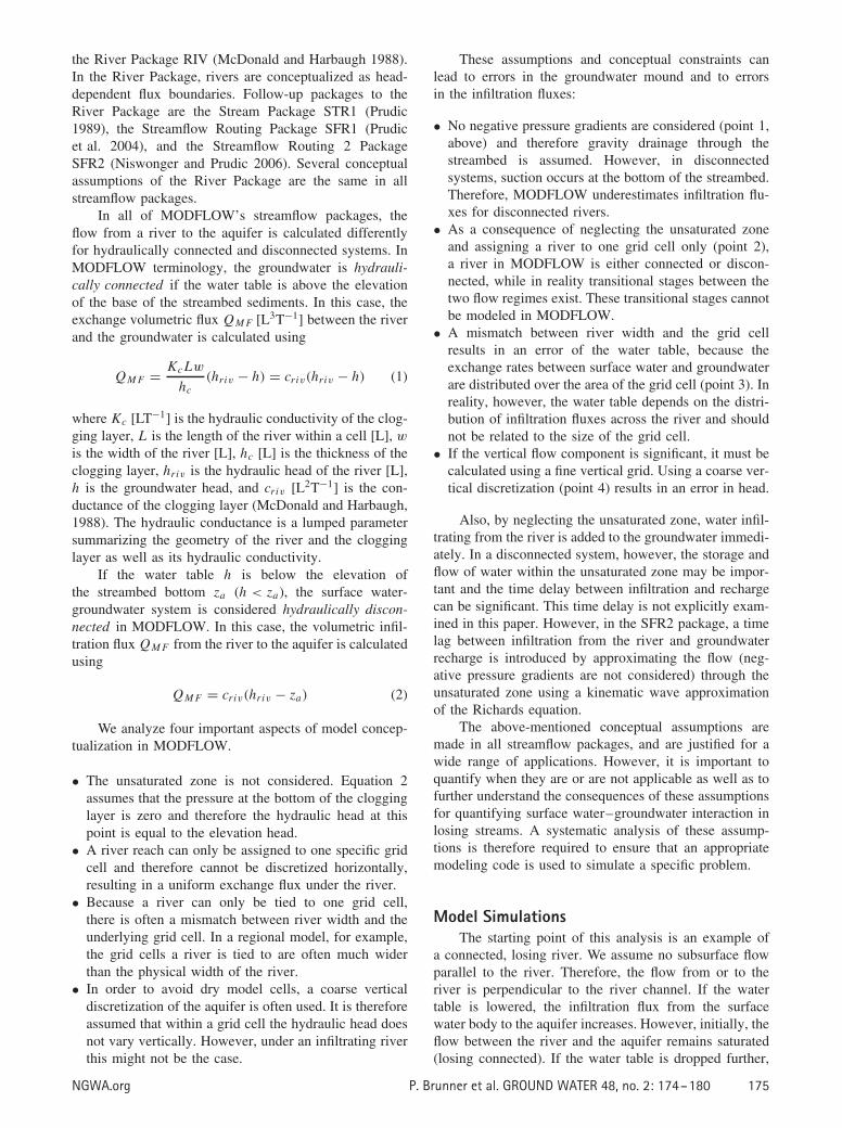
In the following, we simulate the relation betweendifferent stages of the water table and the infiltration rateunder a straight river (this corresponds to the examplestudied in Brunner et al. [2009a]) with both MODFLOW2000 (Harbaugh et al. 2000) and HydroGeoSphere (HGS)(Therrien et al. 2006). The simulations are all steady stateand therefore represent a series of different flow regimesbetween connected and disconnected. We carry out allof our MODFLOW calculations using the River Pack-age because most of the assumptions we discuss for thispackage apply to all USGS streamflow packages. HGSsimulates both saturated and unsaturated flow. The abilityof HGS to simulate flow in the unsaturated zone usingthe Richards equation as well as the disconnection of sur-face water and groundwater has been tested in Brunneret al. (2009a). Moreover, Brunner et al. (2009a) comparedthe free water surface under an infiltrating layer calcu-lated with HGS and an analytical solution (Schmitz andEdenhofer 2000) not based on any form of linearization.The agreement between the two approaches was excellent.HGS is therefore considered as the control experiment forcomparison in this paper. Figure 1 shows the basic modelsetup.

In the variably saturated formulation set up in HGS,a relation between pressure and hydraulic conductivitydescribing the unsaturated zone has to be defined. Weused the van Genuchten approach with the parametersα = 14.5 m−1 and β = 2.68. These parameters are typicalvalues for sand (Carsel and Parrish 1988). The river inHGS is represented as a constant head boundary above theclogging layer. This is an identical approach to the RiverPackage in MODFLOW. In order to correctly simulate theunsaturated zone, the aquifer must be finely discretizedvertically in HGS. In MODFLOW, there are limits to thevertical discretization because model cells can fall dry (theissue of dry cells is discussed later). In order to quantifythe impact of the coarse discretization in MODFLOW, themodel set up in HGS is discretized finer both horizontally(�x = 1 m) and vertically (with a vertical discretizationof 10 cm between z = 115 m and z = 120 m and with 5m between z = 0 m and z = 115 m).

The uniform horizontal discretization �x of themodel domain in MODFLOW is 10 m and is equal tothe width of the river. Vertically, the MODFLOW modelis discretized with 12 layers each of 10 m thickness. Themodel length in the direction of the river is 10 m (�y),represented by a single row. The aquifer is 120 m highin the z direction and the elevation of the bottom of theclogging layer za is also 120 m. The hydraulic conductiv-ity of the aquifer Ka is set to 1 m/d. Homogeneous andisotropic conditions are assumed. The height of the clog-ging layer hc is 0.3 m, and its hydraulic conductivity Kc is0.1 m/d. The depth d of the river is 0.5 m and its width w

is 10 m. The river is straight, leading to a river length of10 m. For some simulations, HGS is not used but insteaddifferent setups within MODFLOW are constructed andcompared. The differences to the initial setup describedabove are mentioned in the corresponding paragraphs.

For both HGS and MODFLOW simulations the headat the lateral boundary is lowered and the steady-stateinfiltration rate is calculated. The system is initially losingconnected. The head at the lateral boundary is lowereduntil the river is disconnected from the groundwater. Thegroundwater is disconnected from the surface water whenthe infiltration flux no longer significantly changes inresponse to a falling water table. In MODFLOW, thisis the case as soon as the water table drops below theelevation of the riverbed bottom. In Figure 2, the effectof lowering the head at the lateral boundaries for thetwo models is illustrated. In HGS, the groundwater isnot disconnected as the water table begins to fall belowthe bottom of the clogging layer. Rather, a transitionbetween connected and disconnected is present and thesystem in HGS is considered disconnected when anadditional increase of �H no longer significantly changesthe infiltration rate. In the transition between connectedand disconnected flow, the flow regime between theriver and the groundwater is partly unsaturated while theinfiltration rate remains a function of the water table (Foxand Durnford 2003). Brunner et al. (2009a) showed that

Figure 1. Model setup used in both MODFLOW and HGS.The horizontal extent of the model is 250 m. The datum z = 0is defined in the lower left corner. Constant head boundariesare defined at the edges of the model domain between z = 0and z = h0 . The midpoint of the river is defined in the centerof the model domain. We assigned the entire model domaina thickness of 10 m.

176 P. Brunner et al. GROUND WATER 48, no. 2: 174–180 NGWA.org

Figure 2. Steady-state infiltration rates of the river as afunction of �H calculated in MODFLOW and HGS. �His the difference between the hydraulic head at the constanthead boundary and the elevation of the top of the aquifer.Point A represents the beginning of the transition zone(beginning of desaturation at the edge of the river). At pointB, disconnection is reached.

this transition is related to both the buildup of a capillaryzone (negative pressure gradients) above the water tableas well as to the geometric properties of the river. Brunneret al. (2009b) showed that different transitional pathwaysexist and that they can significantly influence how changesin the water table affect the infiltration rates.

Compared to MODFLOW, the simulations carriedout with HGS show a higher infiltration flux at full discon-nection and the transition between connected and discon-nected is smooth. Some of the above-mentioned assump-tions and conceptual aspects of MODFLOW explain thetwo differences between MODFLOW and HGS. In thefollowing, we discuss and quantify these assumptions ingreater detail.

Underestimation of InfiltrationIn MODFLOW’s stream and river packages (includ-

ing SFR2), the unsaturated zone is modeled without con-sidering negative pressure gradients. However, if an unsat-urated zone is present under the clogging layer, a suctionγp [L] occurs and this suction increases the flux throughthe clogging layer. Using Darcy’s law,

q = Kc

hc

(hriv − za − γp) = Kc

hc

(hc + d − γp) (3)

where za − γp is the hydraulic head below the streambedsediments, and so the left-hand side of this equation issimply Darcy’s law for flow through the streambed sedi-ments. The difference between the hydraulic head of theriver hriv and the elevation of the bottom of the clogginglayer za is equal to the sum of the river depth d and theheight of the clogging layer hc. In MODFLOW, γp iszero and Equation 3 reduces to Equation 2. Therefore, ifthe values of hydraulic conductivity of the streambed andits geometrical properties are available and used as inputdata, the infiltration flux will be underestimated in theRiver Package if an unsaturated zone is actually present.

Figure 3. Illustration of the influence of neglecting thesuction under the clogging layer for disconnected systems.The relative flux shown on the y-axis is the ratio of theinfiltration flux of a disconnected system calculated byMODFLOW (γ ∗

p = 0) to the infiltration flux calculated witha model considering the unsaturated zone. The aquifermaterial was assumed to be sand. For better readability,only five of the nine possible parameter combinations areshown in this graph.

In practice, values of streambed hydraulic conductivityand its vertical extent are hard to determine and are oftenunknown.

It is apparent from Equation 3 that neglecting theunsaturated zone is justified only if |γp| � hc + d. InFigure 3, the influence of neglecting the suction underthe clogging layer on the infiltration rate of a disconnectedsystem is illustrated for different combinations of d, hc

and Kc. The suction γ that occurs at disconnection isdefined as γ ∗

p . The parameters used in the van Genuchtenequations (van Genuchten 1980) are based on Carsel andParrish (1988) (α = 14.5 m−1 and β = 2.68, Ka =7.1m/d. A relatively large value of Ka was chosen todemonstrate this effect because it is less noticeable if Ka

is close to Kc).The magnitude of γ ∗

p depends on the soil type, thesaturated hydraulic conductivity of the aquifer, and thegravity flux through the clogging layer. γ ∗

p is alwayslarger than the air entry value of the aquifer material. Inthe parameter combinations we presented in Figure 3, theunderestimation of flow is up to a factor of 1.85 (relativeflux 0.54). Osman and Bruen (2002), however, discussedparameter combinations where the decrease was about afactor of three. The effect of the unsaturated zone willdiminish when the river is deep or the clogging layer isthick. In the range of the simulations we carried out, theincrease of flux as a result of suction was small (5% oreven less) when the sum of the river depth and the heightof clogging layer river was above 1 m.

Uniform Infiltration Rates under a River and Absence ofTransition Zone

If a river in MODFLOW is represented with a sin-gle cell it is either completely connected or completelydisconnected. In two and three dimensions, however, a

NGWA.org P. Brunner et al. GROUND WATER 48, no. 2: 174–180 177

Figure 4. Pressure distribution across the river between−w /2 and w /2 (in this case river width w = 10 m) measuredat the bottom of the clogging layer for different values of�H for MODFLOW and HGS. HGS gives a distributionof pressure under the riverbed, while MODFLOW presentsonly one data point. In the HGS simulation shown for �H =4 m, different states of connection under the clogging layercan be identified. In this case, at the edge of the river, the flowis unsaturated (γp < 0), while the flow in the center remainssaturated (γp > 0). The model setup and the parameters arethe same as shown in Figure 1.

groundwater mound develops under the recharging sur-face water body, and the pressure distribution is a func-tion of the location under the riverbed. This nonuniformpressure distribution causes different states of connectionat different points in space and manifests itself as anextended transition zone. The pressure distribution underthe clogging layer is uniform only when a system is dis-connected. Figure 4 illustrates these differences.

In the simulations shown in Figure 4 it is apparentthat the pressure head in MODFLOW is very close tothe average pressure head under the clogging layer forHGS. The results of many simulations (considering a widerange of different parameter combinations, including widerivers with a large transition zone) suggest that the averagepressure in MODFLOW was close to the average valueof the finely discretized HGS model. The difference ofthe infiltration flux for different values of �H could beexplained as a result of neglecting γp in MODFLOW andis only marginally related to the assumption of uniformpressure under the clogging layer. This suggests that theassumption of uniform pressure does not significantlyinfluence the total exchange flux, and for many regionalmodels this assumption is therefore justified. However, themissing horizontal discretization within a river cell has aneffect on the groundwater mound if the physical width ofthe river does not exactly match the width of the rivercell, as described below. (We are aware that it is possibleto represent a river as a series of parallel rivers tied to aseries of grid cells, allowing for horizontal discretizationin the River Package. In all other streamflow packages,however, the river depth is calculated and not prescribedand splitting a river up into several parallel rivers is notstraightforward.)

As illustrated in Figure 2, the MODFLOW simu-lations do not feature a transition between connectedand disconnected regimes. As mentioned above, thereare two reasons for this difference: The first one is theabsence of negative pressures in MODFLOW. As thewater table drops below the clogging layer, the infiltrationrates continuously approach their maximum values. Thisis a smooth function and cannot be reproduced in a modelthat does not consider capillary pressure gradients. Thesecond reason is due to the absence of horizontal dis-cretization of the river. Therefore, in MODFLOW a riveris either fully connected or fully disconnected while inreality the state of connection can vary across a river.

Error in Water Table due to Mismatch of River Widthand Grid Cell Size

There is often a mismatch between the river width w

and the width of a grid cell �x. (In fact, there is always amismatch in a finite difference scheme if the river is notstraight.) While the volumetric infiltration flux Q[L3T−1]of a disconnected system is not affected by this mismatch,the infiltration flux q[LT−1] is. This is an importantdifference because the infiltration rate and the geometry ofthe system are the relevant parameters for determining thegroundwater mound under an infiltrating layer. If the areaof the grid cell is much greater than the area of the riverwithin it, then the infiltration flux q[LT−1] and thereforethe height of the groundwater mound beneath the riverwill be underestimated. Because the calculation of theinfiltration flux is based on the head difference betweenthe river and the groundwater, the calculated infiltrationfluxes are systematically biased if the river and cell widthdo not match.

Consider two configurations of a straight river inMODFLOW. The hydraulic parameters are identical, butthe horizontal size of the grid cell the river is tied todiffers. We define the horizontal dimension of the rivercell as a multiple α of the real river width w such that�x = αw. At disconnection, the volumetric infiltrationQ is independent of α while the infiltration rate q is afunction of α:

q = Q

�x�y= Q

αw�y(4)

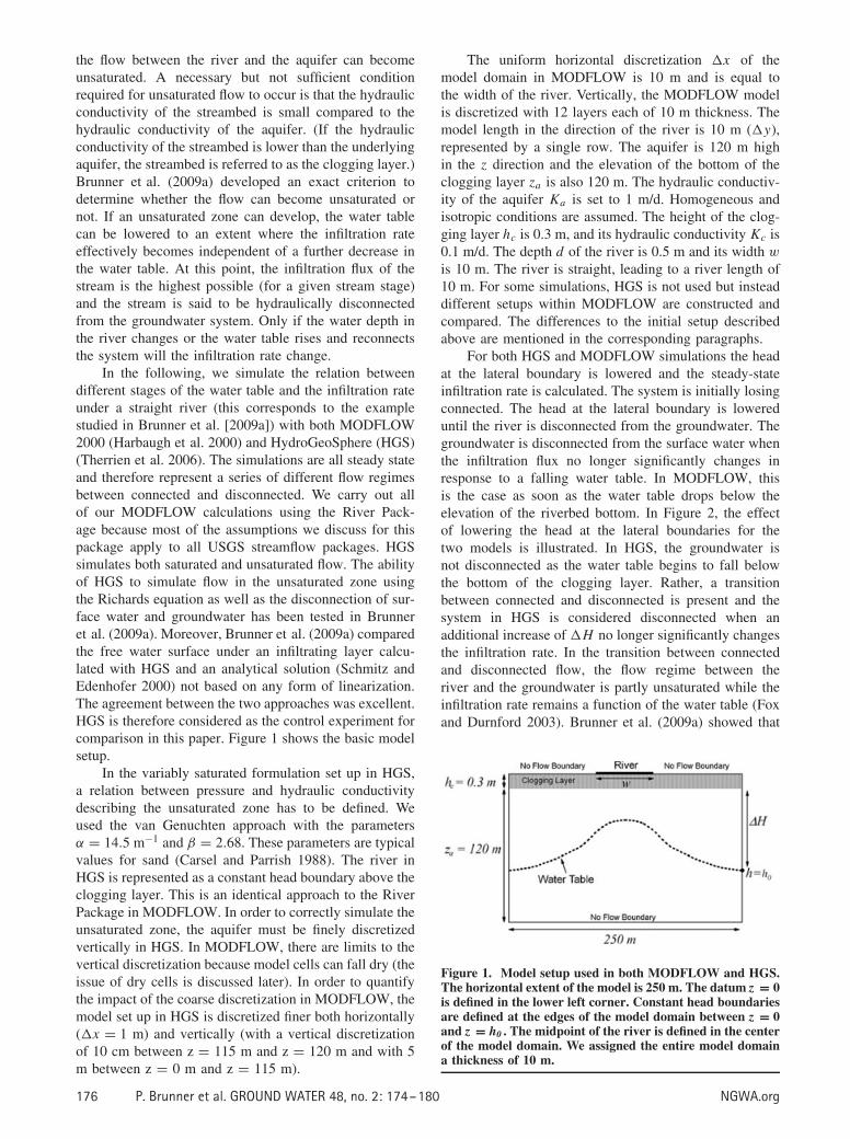
It is readily apparent from Equation 4 that differentvalues of α influence the infiltration rate q and hencethe groundwater mound. In Figure 5, the hydraulic headunder an infiltrating layer of the width w is plotted as afunction of x for different values of α. If the river is tiedto a grid cell with a width smaller than the river (α < 1),the height of the mound under the river is overestimated.If the width of the grid cell is larger than the width of theriver (α > 1), the mound is underestimated. In a typicalregional model, α is larger than 1. The largest error inhead is made directly beneath the center of the river.For illustrative purposes, some parameters in Figure 5deviate from the ones used to generate Figures 3 and 4:L = 500 m, w = 20 m, d = 0.4, hc = 0.4, Kc = 0.1 m/d,Ka = 1 m/d. All other parameters as well as the vertical

178 P. Brunner et al. GROUND WATER 48, no. 2: 174–180 NGWA.org

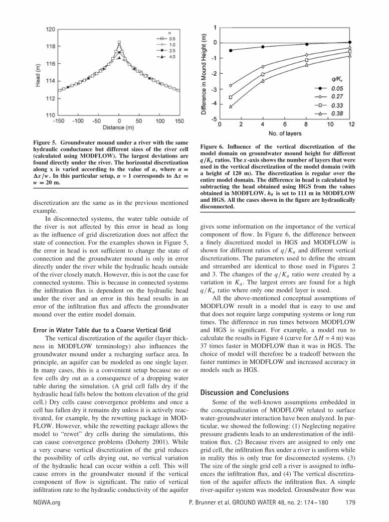
Figure 5. Groundwater mound under a river with the samehydraulic conductance but different sizes of the river cell(calculated using MODFLOW). The largest deviations arefound directly under the river. The horizontal discretizationalong x is varied according to the value of α, where α =�x/w . In this particular setup, α = 1 corresponds to �x =w = 20 m.

discretization are the same as in the previous mentionedexample.

In disconnected systems, the water table outside ofthe river is not affected by this error in head as longas the influence of grid discretization does not affect thestate of connection. For the examples shown in Figure 5,the error in head is not sufficient to change the state ofconnection and the groundwater mound is only in errordirectly under the river while the hydraulic heads outsideof the river closely match. However, this is not the case forconnected systems. This is because in connected systemsthe infiltration flux is dependent on the hydraulic headunder the river and an error in this head results in anerror of the infiltration flux and affects the groundwatermound over the entire model domain.

Error in Water Table due to a Coarse Vertical GridThe vertical discretization of the aquifer (layer thick-

ness in MODFLOW terminology) also influences thegroundwater mound under a recharging surface area. Inprinciple, an aquifer can be modeled as one single layer.In many cases, this is a convenient setup because no orfew cells dry out as a consequence of a dropping watertable during the simulation. (A grid cell falls dry if thehydraulic head falls below the bottom elevation of the gridcell.) Dry cells cause convergence problems and once acell has fallen dry it remains dry unless it is actively reac-tivated, for example, by the rewetting package in MOD-FLOW. However, while the rewetting package allows themodel to “rewet” dry cells during the simulations, thiscan cause convergence problems (Doherty 2001). Whilea very coarse vertical discretization of the grid reducesthe possibility of cells drying out, no vertical variationof the hydraulic head can occur within a cell. This willcause errors in the groundwater mound if the verticalcomponent of flow is significant. The ratio of verticalinfiltration rate to the hydraulic conductivity of the aquifer

Figure 6. Influence of the vertical discretization of themodel domain on groundwater mound height for differentq/Ka ratios. The x -axis shows the number of layers that wereused in the vertical discretization of the model domain (witha height of 120 m). The discretization is regular over theentire model domain. The difference in head is calculated bysubtracting the head obtained using HGS from the valuesobtained in MODFLOW. h0 is set to 111 m in MODFLOWand HGS. All the cases shown in the figure are hydraulicallydisconnected.

gives some information on the importance of the verticalcomponent of flow. In Figure 6, the difference betweena finely discretized model in HGS and MODFLOW isshown for different ratios of q/Ka and different verticaldiscretizations. The parameters used to define the streamand streambed are identical to those used in Figures 2and 3. The changes of the q/Ka ratio were created by avariation in Ka . The largest errors are found for a highq/Ka ratio where only one model layer is used.

All the above-mentioned conceptual assumptions ofMODFLOW result in a model that is easy to use andthat does not require large computing systems or long runtimes. The difference in run times between MODFLOWand HGS is significant. For example, a model run tocalculate the results in Figure 4 (curve for �H = 4 m) was37 times faster in MODFLOW than it was in HGS. Thechoice of model will therefore be a tradeoff between thefaster runtimes in MODFLOW and increased accuracy inmodels such as HGS.

Discussion and ConclusionsSome of the well-known assumptions embedded in

the conceptualization of MODFLOW related to surfacewater-groundwater interaction have been analyzed. In par-ticular, we showed the following: (1) Neglecting negativepressure gradients leads to an underestimation of the infil-tration flux. (2) Because rivers are assigned to only onegrid cell, the infiltration flux under a river is uniform whilein reality this is only true for disconnected systems. (3)The size of the single grid cell a river is assigned to influ-ences the infiltration flux, and (4) The vertical discretiza-tion of the aquifer affects the infiltration flux. A simpleriver-aquifer system was modeled. Groundwater flow was

NGWA.org P. Brunner et al. GROUND WATER 48, no. 2: 174–180 179

assumed to be perpendicular to the river, allowing for a2-D conceptualization. The aquifer was assumed to behomogeneous and isotropic and the analyses are steadystate. We are aware that this setup is simplified, but theissues that are noted in this paper do not change within amore complex system. For example, a mismatch betweenriver width and cell width will result in differences inthe infiltration rate, irrespective of whether the aquiferis homogeneous or heterogeneous or the system is tran-sient or in steady state. Even though all our simulationsare for losing streams, the considerations on vertical dis-cretization of the aquifer and the horizontal discretizationof the river are also relevant for gaining streams. How-ever, additionally complexities arise in the simulation ofgaining streams (e.g., seepage along the riverbank). Mostof the conceptual considerations we have described abovecan go unseen through calibration. This can be problem-atic because the model will produce biased predictions ifit is used in any situation other than those for which itwas calibrated.

AcknowledgmentsThis work was financed by the National Water

Commission in Australia and the Flinders Research Centrefor Coastal and Catchment Environments. Their support isgreatly appreciated. We wish to thank David Prudic, RichNiswonger, and Ian Jolly for their extensive comments ona draft of this paper. George Zyvoloski and an anonymousreviewer provided important feedback in their reviews andhelped to improve the manuscript.

ReferencesBarlow, P.M., and A. Harbaugh. 2006. USGS directions in

MODFLOW development. Ground Water 44, no. 6:771–774.

Brunner, P., P.G. Cook, and C.T. Simmons. 2009a. Hydroge-ologic controls on disconnection between surface waterand groundwater. Water Resources Research 45, W01422,doi10.1029/2008WR006953.

Brunner, P., C.T. Simmons, and P.G. Cook. 2009b. Spatialand temporal aspects of the transition from con-nection to disconnection between rivers, lakes and

groundwater. Journal of Hydrology 376, no. 1–2: 159–169,doi10.1016/j.jhydrol.2009.07.023.

Carsel, R.F., and R.S. Parrish. 1988. Developing jointprobability-distributions of soil-water retention character-istics. Water Resources Research 24, 755–769.

Doherty, J. 2001. Improved calculations for dewatered cells inMODFLOW. Ground Water 39, 863–869.

Fox, G.A., and D.S. Durnford. 2003. Unsaturated hyporheiczone flow in stream/aquifer conjunctive systems. Advancesin Water Resources 26, 989–1000.

Furman, A. 2008. Modeling coupled surface-subsurface flowprocesses: A review. Vadose Zone Journal 7, no. 2:741–756.

Harbaugh, A., E. Banta, M. Hill, and M. McDonald. 2000.MODFLOW-2000, the USGS Modular Groundwater-Model: Users guide to modularization concepts and thegroundwater flow process. U.S. Geological Survey Open-File Report 00-92. Reston, Virginia: USGS.

McDonald, M.G., and A.W. Harbaugh. 1988. A modular, three-dimensional finite-difference ground-water flow model.Reston, Virginia: USGS.

Niswonger, R.G., and D.E. Prudic. 2006. Documentation of thestreamflow-routing (SFR2) package to include unsaturatedflow beneath streams—A modification to SFR1. U.S.Geological Survey Techniques and Methods, Book 6, Chap.A13. Carson City, Nevada: USGS.

Osman, Y.Z., and M.P. Bruen. 2002. Modelling stream-aquiferseepage in an alluvial aquifer: An improved losing-streampackage for MODFLOW. Journal of Hydrology 264, no.1–4: 69–86.

Prudic, D.E. 1989. Documentation of a computer program tosimulate stream-aquifer relations using a modular, finite-difference, ground-water flow model. U.S. Geological Sur-vey Open-File Report 88-729. Carson City. Nevada: USGS.

Prudic, D.E., L.F. Konikow, and E.R Banta. 2004. A new streamflow routing (SFR1) package to simulate stream-aquiferinteraction with MODFLOW-2000. U.S. Geological SurveyOpen-File Report 2004-1042. Carson City, Nevada: USGS.

Schmitz, G.H., and J. Edenhofer. 2000. Exact closed-form solu-tion of the two-dimensional Laplace equation for steadygroundwater flow with nonlinearized free-surface boundarycondition. Water Resources Research 36, 1975–1980.

Therrien, R., R.G. McLaren, E.A. Sudicky, and S.M Panday.2006. Hydrogeosphere. Waterloo, Canada: GroundwaterSimulations Group, University of Waterloo.

van Genuchten, M.T. 1980. A closed-form equation for predict-ing the hydraulic conductivity of unsaturated soils. Soil Sci.Am. Journal 44, 892–898.

180 P. Brunner et al. GROUND WATER 48, no. 2: 174–180 NGWA.org