modeling solute transport in a water repellent soil

Modeling solute transport in a water repellent soil

H.V. Nguyena,* , J.L. Niebera, P. Oduroa, C.J. Ritsemab, L.W. Dekkerb, T.S. Steenhuisc

aDepartment of Biosystems and Agricultural Engineering, University of Minnesota, St. Paul, MN, USAbDLO Winand Staring Centre for Integrated Land, Soil and Water Research, Wageningen, The Netherlands

cDepartment of Agricultural and Biological Engineering, Cornell University, Ithaca, NY, USA.

Received 9 May 1998; accepted 24 August 1998

Abstract

A bromide tracer was applied on a 2.2 m long and 0.4 m wide plot at the location of a hydrophobic soil in the southwest ofThe Netherlands. At the end of the experiment, the plot was excavated to a depth of 0.7 m using 100 cm3 samples, yielding atotal of 1680 samples to quantify the three-dimensional spatial distribution of water content, pH, bromide concentration anddegree of water repellency. Measured water content and solute distributions indicated that unstable (fingered) flow prevails. It isconsidered that contaminant transport under such conditions can proceed at rates that are higher than that which would normallyoccur if the flow were stable. This article illustrates an attempt at modeling contaminant transport under unstable flowconditions using measurements obtained from the experimental plot. A finite element solution of the two-dimensional Richardsequation forms the basis for the unstable flow simulation, while a particle tracking random walk solution of the two-dimensionalconvection–dispersion equation forms the basis of the transport simulation. The water flow simulation and the solute transportsimulation were compared with the measured data. Initial results indicate that model predictions compared fairly well withmeasured water content and solute transport data.q 1999 Elsevier Science B.V. All rights reserved.

Keywords:Unstable flow; Preferential flow; Hydrophobic soil; Solute transport; Particle tracking method

1. Introduction

The contamination of groundwater by substancesfrom various point and non-point sources is a signifi-cant problem. Many aquifers have been invaded byanthropogenic chemicals resulting from leaky under-ground storage tanks, chemical spills, waste landfillsand agricultural production. These pose dangers to thedrinking water resources in many parts of the world.Numerical simulation models offer an effective toolfor predicting the movement of contaminants andevaluating the sensitivity of the governing contaminant

transport processes to their inherent systemparameters.

In recent times however, models based on diffusetypes of flows and solute transport have often beenfound to be incapable of simulating actual waterflow and solute transport. The occurrence of prefer-ential flow is the main reason for this shortcoming(Ritsema and Dekker, 1998). Preferential flow gener-ally occurs when there are macropores, but in theabsence of macropores it has been observed to occurwhen conditions that promote instability at thewetting front are present (Hill and Parlange, 1972;Diment et al., 1982; Glass et al., 1988; Ritsema andDekker, 1994). In the latter case, the resulting flow istermed unstable.

When unstable flow occurs, water and solutes move

Journal of Hydrology 215 (1999) 188–201

0022-1694/99/$ - see front matterq 1999 Elsevier Science B.V. All rights reserved.PII: S0022-1694(98)00270-4

* Corresponding author. Tel.:1 1-612-625-6724; Fax:1 1-612-624-3005; e-mail: hnguyen@s1./arc.umn.edu

in preferential pathways through the vadose zone atvelocities that are close to the saturated pore velocity(Glass et al., 1988). This by-passing flow can signifi-cantly increase the amount of harmful substancesmoving to the underlying groundwater (Glass et al.,1988), and also cause a reduction of nutrients andwater available for plant growth (Jamison, 1945).Thus, it is necessary to develop tools for modelingsolute transport under unstable flow conditions forpossible incorporation into existing models.

In the development of models for simulatingunstable flow, Nieber (1996) proposed a numericalsolution scheme of the Richards equation to modelunstable flow. He showed that the model was capableof predicting finger widths that were similar to thoseobtained from analytical theory. Nguyen et al. (1999)successfully demonstrated modeling of unstable flowusing the methodology of Nieber (1996) for fieldconditions.

The purpose of this article is to report on attemptsto simulate solute transport patterns observed in thefield under unstable flow conditions in a waterrepellent soil. The simulation of the observed wettedpatterns is achieved with a finite element solution ofthe two-dimensional Richards equation. Solutetransport is modeled using the random walk particle

tracking (RWPT) model to solve the convection–dispersion equation. The particle tracking methodhas the advantage (over finite difference approxima-tions and finite element methods) of being able toovercome numerical dispersion and artificial oscilla-tions associated with sudden spatio–temporal changesin solute concentration (Abulaban et al., 1998).Clearly, modeling solute transport under unstableflow conditions will involve sudden changes in soluteconcentration at the wetting front. In this article,model results are compared with field measured datafrom a bromide tracer experiment on a water-repellentsoil in The Netherlands.

2. Materials and methods

2.1. Field experiments

2.1.1. SoilThe experimental site is located near Ouddorp in

the southwestern part of The Netherlands. The soilconsists of approximately 10 cm organic rich topsoilupon fine medium dune sand, and has been classifiedas a Typic Psammaquent (De Bakker, 1979). Beneaththe humic layer, the soil is water repellent to a depth

H.V. Nguyen et al. / Journal of Hydrology 215 (1999) 188–201 189

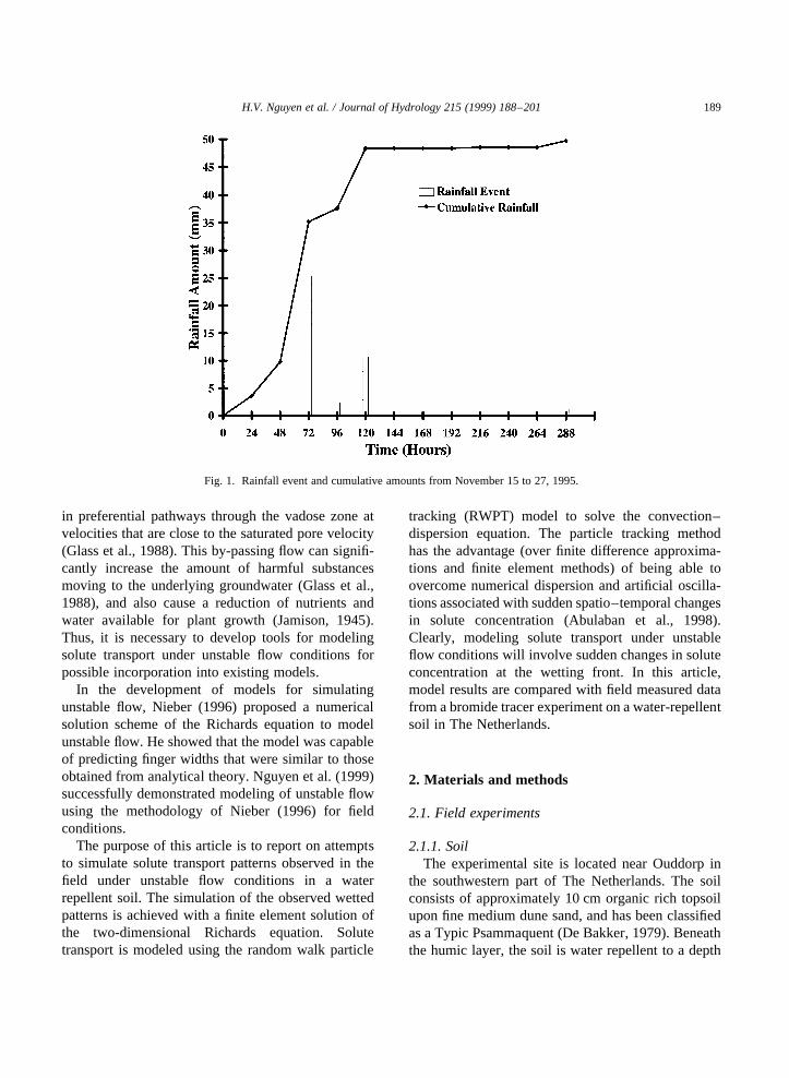
Fig. 1. Rainfall event and cumulative amounts from November 15 to 27, 1995.

of more than 50 cm. The experimental site is grasscovered, and was previously used in a detailed TDRexperiment on finger formation and finger recurrenceusing an automated TDR measuring device (Ritsemaet al., 1997a), and a subsequent modeling study(Nguyen et al., 1999).

2.1.2. Tracer experimentThe experimental plot was 2.2 m long and 0.4 m

wide. A KBr tracer solution was applied manuallyto the soil surface with six nozzle sprinklers onNovember 15, 1995. The tracer application rate wasdetermined by placing 24 small trays around theexperimental plot. An average of 8.0 g bromide perm2 was applied, with a standard deviation of 1.5 g/m2.On November 27, after 52 mm of rain, excavation ofthe experimental plot was performed, according to aspatial grid of 40× 6 × 7 samples, in thex, y andzdirections, respectively, yielding a total of 1680samples for the entire plot. Samples were taken byusing steel cylinders (5 cm high by 5 cm diameter;or about 100 cm3 volume), which were carefullypushed into the soil. In the horizontal direction, theseparation distance between two adjacent sampleswas 0.5 cm. Seven soil layers were sampled at depthintervals of 0–5, 9–14, 19–24, 30–35, 42–47, 55–60,and 69–74 cm. The samples were taken to the labora-tory for the determination of soil water content,degree of water repellency, soil pH, and bromideconcentration. In this article, soil water content andbromide concentration distributions will be used.

Rainfall and groundwater levels were recordedautomatically from November 15 to 27. A total of52 mm of rain was recorded in this period, and thegroundwater table rose from a depth of about 174 to170 cm below the soil surface. A plot of the rainfallevent and cumulative rainfall amount are shown inFig. 1.

2.2. Laboratory measurements

All field-moist soil samples were first weighed inthe laboratory, and the degree of actual water repel-lency was determined using the water drop penetra-tion time (WDPT)-test described by Dekker andRitsema (1994). Thereafter, samples were oven-dried at 658C, and weighed again to determine thevolumetric soil water content. The samples were

then used to determine bromide concentrations.After adding water to the samples, and shaking for afixed period of time, bromide concentration in thesolution was measured using the High Pressure LiquidChromatography technique.

2.3. Numerical methods

2.3.1. Numerical method for unstable flowThe numerical simulation of the flow of water in the

experimental trench is based on a finite element solu-tion of the two-dimensional Richards equation. Thederivation of the finite element equations waspresented by Nieber (1996). Details of the applicationof this numerical solution to the experimental trenchwere presented by Nguyen et al. (1999).

The numerical solution to the Richards equationprovides data on the distribution of water pressureand water saturation in the soil profile. To performthe solute transport simulation, it is necessary tocompute the pore velocities within the flow domain.These velocities are derived from the finite elementsolution results by applying Darcy’s law as:

uvx � 2K2hw

2x; �1a�

uvz � 2K2hw

2z2 K; �1b�

whereu is the volumetric water content,vx andvz arethe horizontal and vertical velocities,K is the unsatu-rated hydraulic conductivity,hw is the water pressure,andx andz are the horizontal and vertical Cartesiancoordinates, respectively.

2.3.2. Numerical method for solute transportThe transport of a non-sorbing solute can be solved

numerically using the convection–dispersion equa-tion (CDE) under unsaturated conditions. It is writtenas:

2uC2t

1 7·�uCv�2 7·�D·u7C� � 0; �2�whereC is the solute concentration in the liquid phase,D the hydrodynamic dispersion tensor defined by Eq.(3),v is the local velocity vector, andt is the time. Thehydrodynamic dispersion tensor is given by

D � �aTV 1 Dm�I 1 �aL 2 aT� vvV

; �3�

H.V. Nguyen et al. / Journal of Hydrology 215 (1999) 188–201190

whereaL andaT are the longitudinal and transversedispersivities respectively,V is the magnitude of thevelocity vector,Dm is the molecular diffusion coeffi-cient, I is the identity matrix, andvv is the diadic ofthe velocity vector.

The RWPT method can be used to obtain a solutionto Eq. (2). In this method, a mass of solute is repre-sented by a finite number of discrete particles thatmove with a convective force represented by thelocal velocity field, and a dispersive component thatis represented as a random movement. To solve theCDE by the RWPT method, Eq. (2) may be rear-ranged in a form similar to the Fokker–Planck equa-tion, that is,

2�uC�2t

1 7· uC�v 11u

D·7u��

2 7·{ D·7�uC�} � 0:

�4�The Fokker-Planck equation is given by Eq. (5)

(Tompson et al., 1988), and is a conservation equationfor the probability distribution of particles movingindependently in a random field.

2f2t

1 7· fA 2 7·12

BBT� ��

2 7·12

BBT·7f� �

� 0:

�5�In Eq. (5),f(X,t) is the probability density of parti-

cles expected to be found around a locationX at timet, X(t) is the position of a particle at timet, A(X,t) isthe vector used to represent the deterministic drivingforce acting to changeX, andB(X,t) is a second ordertensor aligning the random forces acting on the parti-cle with A. The location of a particle,i, that moves ina random field at timet, can be described by the inte-grated form of the non-linear Langevin equation(Gardiner, 1985) over a time stepDtm as

Xm;i � Xm21;i 1 A iDtm 1 BiRm;i

��Dtm

p; �6�

where the subscriptm indicates the time level,Xm,i

andXm21,i are subsequent locations of particlei overa time intervalDtm ( � tm 2 tm21). In this article, thevectorRm,i is represented by a simple uniform distri-butionU�^ ��

3p � for each component,Rm,j,i (j � x,z) of

Rm,i.Comparison of Eq. (2) with Eq. (5) indicates that

the termsA andB must be chosen such that

f � uC; �7a�

BBT � 2D �7b�

A � v 1 7· D 11u

D·7u: �7c�

If a large number of particles represent a fixedamount of total solute mass, then the location of anyparticle can be found in the form of a stepping equa-tion as

Xm;i � Xm21;i 1

�v�Xm21;i ; tm�1 7· D�Xm21;i ; tm�

11u

D�Xm21;i ; tm�·7u�Dtm

1 B�Xm21;i ; tm�Rm;i

��Dtm

p �8�A more detailed explanation of the solution tech-

nique of RWPT method can be found in Tompson etal. (1988) and Abulaban et al. (1998). Abulaban et al.(1998) developed a RWPT code for solute transport insaturated porous media. For use in the present study,this code was modified to accommodate the simula-tion of solute transport in unsaturated porous media,that is the solution of Eq. (2). Conditions for bothinstantaneous sources and continuous sources ofsolute were accommodated in the code. Ahlstrom etal. (1977) discusses in detail the application of themethod to the case of a continuous source. The parti-cles were uniformly initiated in the top boundary andcould leave the domain only at the bottom boundaryduring the simulation period.

2.4. Model evaluation

To determine how well the numerical simulationsof flow and solute concentrations mimic the observedfield data, visual comparisons of observed and simu-lated patterns of wetting and solute concentrationwere performed. In addition, three statistical measuresof the comparison of the observed and simulatedwater content and solute concentration were calcu-lated. These were the mean difference (MD) betweenthe simulated and observed values, standard deviationfor the mean difference (S) and coefficient of determi-nation (CD). The equations for these measures arepresented by Nguyen et al. (1999) and the backgroundjustification for their use is given by Cooley (1979)and Loague and Green (1991).


3. Modeling of unstable flow and solute transport

As the flow and solute transport models were two-dimensional models, model results will be comparedwith field data from two-dimensional sections (verti-cal slices) of the three-dimensional domain. Thebromide tracer experiment was performed over a 12-d period. At the end of this period, the soil profile was

excavated to measure the distribution of water contentand solute concentration. While model simulations ofsaturation and solute concentration are available overthe 12-d period of the tracer experiment, only the


Fig. 2. Illustration of zonal designation of initial conditionsassigned for the water flow simulation.

Table 1Distribution of number of particles injected during the simulationperiod.

Number of particles

Date Scenario 1 Scenario 2

11/15/95 50 000 355711/16/95 612611/17/95 25 09811/18/95 237111/19/95 10 67211/23/95 19811/26/95 118611/27/95 792

Fig. 3. The spatial distribution of observed saturation for the six sections.

simulated results on the 12th day will be used forcomparison with the field data.

The two-dimensional flow domain (2.2× 0.7 m2)was discretized into 14 000 linear rectangularelements with vertical and horizontal dimensions of0.01 and 0.011 m, respectively. The soil parametersused in the simulations and the implementation of theinitial and boundary conditions are summarized inNguyen et al. (1999). The velocities and volumetricwater content obtained from the unstable flow modelfor all elements were used as input for the solutetransport model.

The initial condition for the water flow simulationrequires assignment of water saturation and positionon the hysteric water retention curve for the soil. The

initial saturation distribution was identical to that usedby Nguyen et al. (1999). Assignment of the initialposition on the water retention curve was based onthe pattern of wetting observed (and simulated) tooccur in the trench as reported by Nguyen et al.(1999). It was assumed that the soil in the zonespreviously wetted (by finger flow) would experiencethe drainage cycle of the water retention curve, whilethe soil in the zones that had remained dry (zonesbetween the fingers) would experience the wettingcycle of the water retention curve. A schematic ofthe assigned zones is shown in Fig. 2. The darkercolor represents portions assigned to the main drai-nage curve and the lighter color, the main wettingcurve. These assigned initial conditions essentially


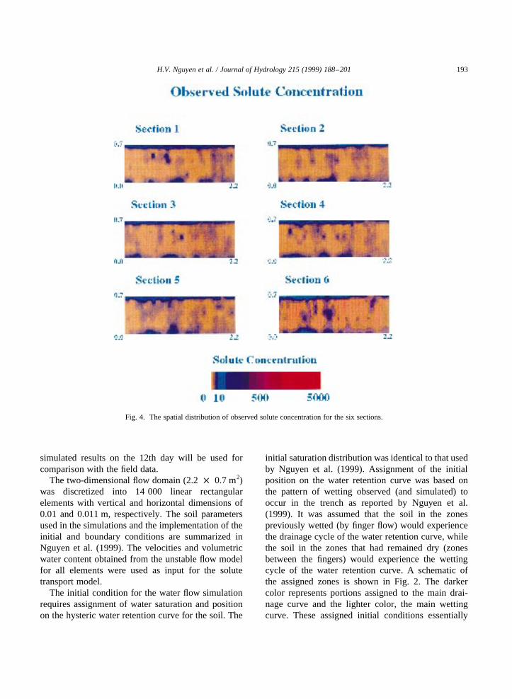
Fig. 4. The spatial distribution of observed solute concentration for the six sections.

predetermine that the water will flow preferentiallydown the previously wetted zone because of fingerpersistence (Glass et al., 1989; Nieber, 1996). As theobjective of this study was to test the preferentialtransport of the solute, this predetermined conditionwas not considered a limitation of the study.

The solute transport simulations were performedseveral times to test the effect of the longitudinal

dispersivity, aL assigned to the discrete elementdomains. Values used ranged between 0.001 and0.01 m, a range in accord with the recommendationsof Fried (1975) and common practice. We found thatusing the value of 0.001 m, led to insufficient spreadof the solute in comparison to the observed solutedistribution. A longitudinal dispersivity of 0.01 myielded solute plumes in much better agreement


Fig. 5. The distributions of simulated saturation at various times and the distribution of average observed saturation for the six sections.

with the measured solute plume and therefore, theresults reported here will be foraL � 0.01 m. Thetransverse dispersivity,aT, was set equal to 0.2aL (�0.002 m), also in accord with the common practice.

The solute mass was represented by 50 000 parti-cles. Two scenarios were run: (1) particles wereinstantaneously injected at the beginning of the simu-lation and (2) particles were successively injected inproportion to the rainfall amount. In the first scenario,the assumption was that all solute were fully mixedwith the initial soil water and transport of the wholemass proceeded immediately upon injection. Inscenario (2), the assumption was based on a sugges-tion to account for the observed high concentration ofbromide in the humic layer. Ritsema and Dekker(1998) proposed that the humic layer acted like areservoir of bromide, releasing it through lateralspreading to the finger pathways for vertical migrationto the bottom of the profile. Successive injection wasthen a means of simulating this ‘‘reservoir ofbromide’’. In both scenarios, the particles wereinitiated from the elements at the surface. Table 1shows the distribution of particle injection over thesimulation period.

4. Results and discussion

4.1. Observed saturation and solute concentration

The observed saturation and bromide concentrationpatterns were displayed for six vertical planes (x–zdomains) in which they-horizontal locations were2.7, 8.5, 14.2, 20.0, 25.7 and 31.5 cm. These sixsections were numbered 1, 2, 3, 4, 5 and 6, respec-tively. The soil water content for the 280 soil samplesfor each section was converted to saturation data.These saturation and solute concentration data wereinterpolated by Kriging method using SURFERTM

software (version 5.0).Illustrations of the observed spatial pattern of

moisture saturation in the six sections are presentedin Fig. 3, while the observed solute concentration inthese sections are presented in Fig. 4. It is seen fromthese plots that the patterns of saturation and soluteconcentration are quite similar in spatial distribution.Most values of solute concentration and saturationwere smaller than 10 g/m3and 0.3, respectively, inthe hydrophobic layer. The saturation and soluteconcentration were high in the humic layer and in


Fig. 6. Observed versus simulated saturation at sampling locations.

the 60–70 cm depth layer relative to the rest of thedomain. The total mass of bromide left in the soilprofile was computed from the six sections to be4.752 g. The total solute mass applied at the surfacewas 7.04 g, and therefore it was estimated that theamount of bromide leached through the bottom ofthe profile was 2.288 g, or 32.5% of the applied mass.

4.2. Simulation of water saturation

Fig. 5 shows the simulated saturation at varioustimes. After 24 h, and 4 mm of rainfall, the infiltratingrainfall had moved into the fingered paths and the

wetting front had already reached the underlyinghydrophilic layer. The water in these fingered path-ways did not diffuse laterally because of the poorwettability of the surrounding hydrophobic media.After 48 h, and 10 mm of cumulative rainfall, theinfiltrating water had penetrated into the underlyinghydrophilic layer and it could be seen that the wettingpattern had spread widely in the hydrophilic layer.These observations were similar to those found inthe field by Ritsema et al., 1993 (see their Fig. 13).

From 48 to 120 h, an additional 40 mm of rainfallaccumulated, and this water continued to move down-ward from the surface through the fingered pathwaysto the hydrophilic layer. Following this rainfall, theprofile drained. In the drained profile, shown at 192 h,it is difficult to distinguish the fingered flow pathsobserved earlier. This indicated that most of thewater had drained within the 120 h following the lastmajor rain event. This generally agrees with theobservations from the field showed by Ritsema et al.,(1997a,b)). Only trace amounts of rain occurred afterthe last major rain event and the redevelopment of thepreferential flow paths barely became visible. Theamount of additional rainfall was too small to promotecomplete renewal of these pathways.

The observed wetted patterns shown in Fig. 3correspond to the simulated saturation patternshown in Fig. 5 at 288 h. In general, both theobserved and simulated saturation patterns showthat the saturation was high in the humic layer andnear the bottom of the soil profile. The biggestdiscrepancies between the observed and simulatedsaturation distributions occur in the hydrophobiclayer. The simulated wetted regions appear to besomewhat wider than those in the observed regions.This may be caused by the fact that in the assignmentof the properties of the hydrophobic layer, it was


Table 2Summary of statistical analyses of differences between simulatedand observed saturation and solute concentration.

Statistic Saturationa Solute concentrationb

MD 0.054 2 5.058S 0.055 7.470CD 0.864 1.078

a n � 280b n � 272.

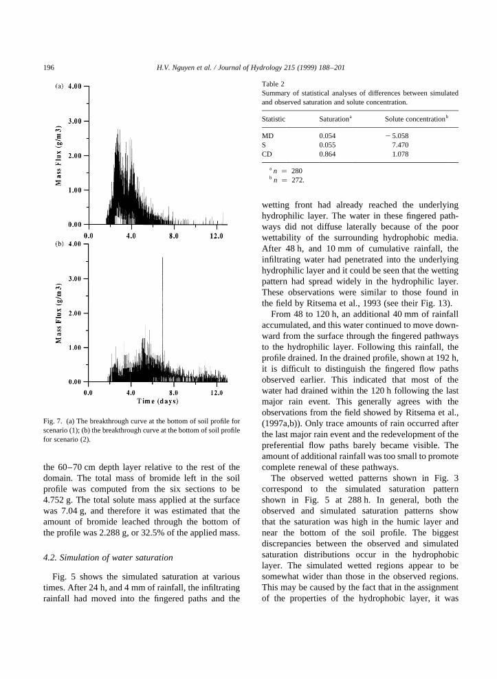
Fig. 7. (a) The breakthrough curve at the bottom of soil profile forscenario (1); (b) the breakthrough curve at the bottom of soil profilefor scenario (2).

assumed that the properties were spatially uniform.We hypothesize that the somewhat narrower wettedzones in the observed saturation distribution may bedue to the fact that the hydrophobic layer has a non-uniform distribution of wettability as shown byRitsema and Dekker (1998).

The observed saturation was sampled at a scale of5 cm in the vertical and horizontal directions, and soto compare with the measured values the simulated

results were averaged over the same scale. A plot ofthe observed versus simulated saturation at thesampling locations is presented in Fig. 6. The averageobserved saturations for the six sections were used forthis plot. As the water content in the soil profile iseither dry (inter-finger zones) or wet (finger zones orhumic layer), the predicted saturation distributedseparately in two zones: low and high saturation(Fig. 6). The difference between simulated and


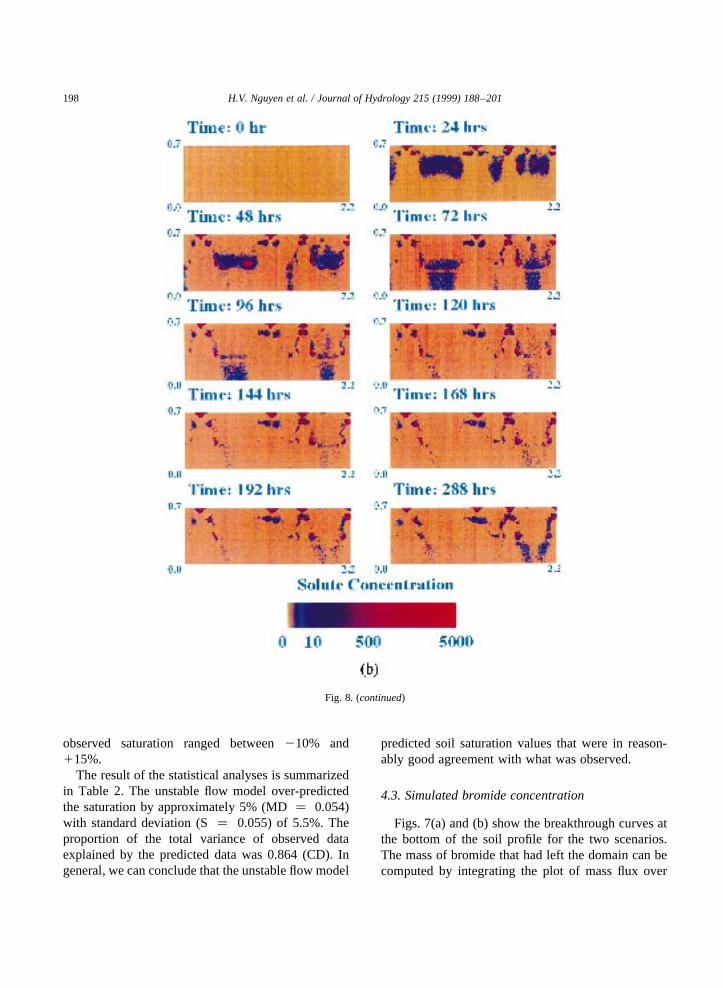
Fig. 8. (a) The spatial distribution of simulated solute concentration for scenario (1); (b) the spatial distribution of simulated solute concentra-tion for scenario (2).

observed saturation ranged between210% and115%.

The result of the statistical analyses is summarizedin Table 2. The unstable flow model over-predictedthe saturation by approximately 5% (MD� 0.054)with standard deviation (S� 0.055) of 5.5%. Theproportion of the total variance of observed dataexplained by the predicted data was 0.864 (CD). Ingeneral, we can conclude that the unstable flow model

predicted soil saturation values that were in reason-ably good agreement with what was observed.

4.3. Simulated bromide concentration

Figs. 7(a) and (b) show the breakthrough curves atthe bottom of the soil profile for the two scenarios.The mass of bromide that had left the domain can becomputed by integrating the plot of mass flux over


Fig. 8. (continued)

time. The amount of bromide leached out of theprofile for both scenarios compared very well withthe observed. For scenario (1), 31.2% of the totalinjected mass left the profile and for scenario (2),27.1% left. These quantities compare quite well withthe observed amount of 32.5%. The breakthroughcurves for the two scenarios differ in the time distri-bution of mass flux leaving the profile. Scenario (1)shows a very prominent peak which tails off appreci-ably towards the end of the simulation period, whilescenario (2) shows a flatter peak which is delayedrelative to scenario (1), has very little variation inthe mass flux, and does not tail off as much towardthe end of the simulation period.

The pattern of simulated solute migration is seen tobe similar to that of the simulated water migration, as

expected. Figs. 8(a) and (b) show the patterns of simu-lated solute concentration at various times for the twoscenarios. The solute particles reached the hydropho-bic layer at 24 h, and some left the bottom of the soilprofile at 48 h in both the scenarios. The mass flux forscenario (1) is higher than that for scenario (2) until120 h. It is reversed after that time. As the saturationand velocity distributions are the same for bothscenarios, the differences between these is owing tothe mode of solute injection for the two scenarios.Visual assessment of the concentration profiles ofthe two scenarios shows that there was little differencebetween them. At the end of the simulation, scenario(1) showed solute remaining in a few spots in thehumic layer, while scenario (2) has solute distributedfairly uniformly within the humic layer. There is moresolute left in the hydrophilic layer for scenario (2)than for scenario (1).

The simulated solute distributions for the twoscenarios at 288 h are presented in Fig. 9, with thedistribution of average solute concentration for the sixsections. There is considerable difference in the pointby point solute concentration between the simulatedand observed solute distributions. In particular, wecan see that there is significantly more solute remain-ing in the humic layer than is found in the simulatedresults, and there seems to be more observed lateralspreading of the solute in the hydrophilic layer thanfound in the simulated results.

The results of the statistical analyses comparing thesolute distributions for scenario (2) at 288 h with theaverage measured results are summarized in Table 2.Scenario (2) was selected because the observed solutedistribution pattern in the humic layer was betterrepresented in this scenario than in scenario (1). Inthe calculation of the statistics for the comparison ofthe simulated and observed solute concentrations,eight of he 280 sampling values were not usedbecause they were extreme outliers (the simulatedvalues were approximately one order of magnitudelarger than the observed). The model underpredictedsolute concentration (MD� 2 5.06). The largevalue of S (7.470) indicates that the variation betweenobserved and simulated solute concentration is high.The proportion of the total variance of observed dataexplained by the predicted data was close to one (CD� 1.078), signifying model performance to be fairlygood. Fig. 10 helps to explain these statistical


Fig. 9. The distribution of simulated solute concentration at 288 hand average measured solute concentration for the six sections.

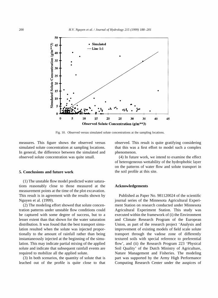
measures. This figure shows the observed versussimulated solute concentration at sampling locations.In general, the difference between the simulated andobserved solute concentration was quite small.

5. Conclusions and future work

(1) The unstable flow model predicted water satura-tions reasonably close to those measured at themeasurement points at the time of the plot excavation.This result is in agreement with the results shown byNguyen et al. (1999).

(2) The modeling effort showed that solute concen-tration patterns under unstable flow conditions couldbe captured with some degree of success, but to alesser extent than that shown for the water saturationdistribution. It was found that the best transport simu-lation resulted when the solute was injected propor-tionally to the amount of rainfall rather than beinginstantaneously injected at the beginning of the simu-lation. This may indicate partial mixing of the appliedsolute and indicate that subsequent rainfall events arerequired to mobilize all the applied solute.

(3) In both scenarios, the quantity of solute that isleached out of the profile is quite close to that

observed. This result is quite gratifying consideringthat this was a first effort to model such a complexphenomenon.

(4) In future work, we intend to examine the effectof heterogeneous wettability of the hydrophobic layeron the patterns of water flow and solute transport inthe soil profile at this site.

Acknowledgements

Published as Paper No. 981120024 of the scientificjournal series of the Minnesota Agricultural Experi-ment Station on research conducted under MinnesotaAgricultural Experiment Station. This study wasexecuted within the framework of (i) the Environmentand Climate Research Program of the EuropeanUnion, as part of the research project ‘Analysis andimprovement of existing models of field scale solutetransport through the vadose zone of differentlytextured soils with special reference to preferentialflow’, and (ii) the Research Program 223 ‘PhysicalSoil Quality’ of the Dutch Ministry of Agriculture,Nature Management and Fisheries. The modelingpart was supported by the Army High PerformanceComputing Research Center under the auspices of


Fig. 10. Observed versus simulated solute concentrations at the sampling locations.

the Department of the Army, Army Research Labora-tory cooperative agreement number DAAH04-95-2-0003/contract number DAAH04-95-C-0008, thecontent of which does not necessarily reflect the posi-tion or the policy of the government, and no officialendorsement should be inferred. Collaboration on theresearch was supported by the NATO CollaborativeResearch Grant No. 960704.

References

Abulaban, A., Nieber, J.L., Misra, D., 1998. Modeling plume beha-vior for nonlinearly sorbing solutes in saturated homogeneousporous media. Advances in Water Resources 21, 487–498.

Ahlstrom, S.W., Foote, H.P., Arnett, R.C., Cole, C.R., Serne, R.J.,1977. Multicomponent mass transport model: theory andnumerical implementation. Report BNWL 2127, Battelle, Paci-fic Northwest Laboratories, Richland WA.

Cooley, R.L., 1979. A method of estimating parameters and asses-sing reliability for models of steady state groundwater flow, 2:application of statistical analysis. Water Resour. Res. 15 (3),603–617.

De Bakker, H., 1979. Major soils and soil regions of the Nether-lands. Junk, Den Haag and Pudoc, Wageningen, the Netherlands.

Dekker, L.W., Ritsema, C.J., 1994. How water moves in a waterrepellent sandy soil. 1. Potential and actual water repellency.Water Resour. Res. 30, 2507–2517.

Diment, G. A., Watson, K.K., Blennerhassett, P.J., 1982. Stabilityanalysis of water movement in unsaturated porous materials, 1.Theoretical considerations. Water Resour. Res. 18, 1248–1254.

Fried, J.J., 1975. Groundwater Pollution. Elsevier, NY.Glass, R.J., Steenhuis, T.S., Parlange, J.-Y., 1988. Wetting front

instability as a rapid and far-reaching hydrologic processes inthe vadose zone. J. Contam. Hydrol. 3, 207–226.

Glass, R.J., Steenhuis, T.S., Parlange, J.Y., 1989. Mechanism forfinger persistence in homogenous, unsaturated, porous media:Theory and verification. Soil Sci. 148, 60–70.

Hill, D.E., Parlange, J.-Y., 1972. Wetting front instability in layeredsoils. Soil Sci. Soc. Am. Proc. 36, 697–702.

Jamison, V.C., 1945. The penetration of irrigation and rain waterinto sandy soils of central Florida. Soil Sci. Soc. Amer. Proc.(10), 25–29.

Loague, K.M., Green, R.E., 1991. Statistical and graphical methodsfor evaluating solute transport models: overview and applica-tion. J. Contam. Hydrology 7, 51–73.

Nguyen, H.V., Nieber, J.L., Ritsema C.J. Dekker, L.W. Steenhuis,T.S. 1999. Modeling gravity driven unstable flow in a waterrepellent soil. J. Hydrol., 215, 202–214.

Nieber, J.L., 1996. Modeling finger development and persistence ininitial dry porous media. Geoderma 70, 209–229.

Ritsema, C.J., Dekker, L.W., Hendrickx, J.M.H., Hamminga, W.,1993. Preferential flow mechanism in a repellent sandy soil.Water Resour. Res. 29, 2183–2193.

Ritsema, C.J., Dekker, L.W., 1994. How water moves in a waterrepellent sandy soil: 2. Dynamics of fingered flow. WaterResour. Res. 30, 2519–2531.

Ritsema, C.J., Dekker, L.W., van den Elsen, E.G.M., Oostindie, K.,Nieber, J.L., 1997. Recurring fingered flow pathways in a waterrepellent sandy field soil. J. Hydrology and Earth SystemSciences 4, 777–786.

Ritsema, C.J., Dekker, L.W., Heijs, A.W.J., 1997. Three-dimen-sional fingered flow patterns in a water repellent sandy fieldsoil. Soil Sci. 162, 79–90.

Ritsema, C.J., Dekker, L.W., 1998. Three-dimensional patterns ofmoisture, water repellency, bromide and pH in a sandy soil. J.Cont. Hydr. 31(3–4): 295–313.

Tompson, A.F.B., Vomvoris, E.A., Gelhar, L.W., 1988 Numericalsimulation of solute transport in randomly heterogeneous porousmedia: motivation, model development and application, Rep #36, Ralph M. Parson Laboratory, Dept. of Civil Eng. Mass Inst.Of Tech. Cambridge, MA.


modeling solute transport in a water repellent soil

Documents