Modeling Interestingness with Deep Neural Networks

Jianfeng Gao, Patrick Pantel, Michael Gamon, Xiaodong He, Li Deng

Microsoft Research

One Microsoft Way

Redmond, WA 98052, USA {jfgao,ppantel,mgamon,xiaohe,deng}@microsoft.com

Abstract

This paper presents a deep semantic simi-

larity model (DSSM), a special type of

deep neural networks designed for text

analysis, for recommending target docu-

ments to be of interest to a user based on a

source document that she is reading. We

observe, identify, and detect naturally oc-

curring signals of interestingness in click

transitions on the Web between source and

target documents, which we collect from

commercial Web browser logs. The DSSM

is trained on millions of Web transitions,

and maps source-target document pairs to

feature vectors in a latent space in such a

way that the distance between source doc-

uments and their corresponding interesting

targets in that space is minimized. The ef-

fectiveness of the DSSM is demonstrated

using two interestingness tasks: automatic

highlighting and contextual entity search.

The results on large-scale, real-world da-

tasets show that the semantics of docu-

ments are important for modeling interest-

ingness and that the DSSM leads to signif-

icant quality improvement on both tasks,

outperforming not only the classic docu-

ment models that do not use semantics but

also state-of-the-art topic models.

1 Introduction

Tasks of predicting what interests a user based on

the document she is reading are fundamental to

many online recommendation systems. A recent

survey is due to Ricci et al. (2011). In this paper,

we exploit the use of a deep semantic model for

two such interestingness tasks in which document

semantics play a crucial role: automatic highlight-

ing and contextual entity search.

Automatic Highlighting. In this task we want

a recommendation system to automatically dis-

cover the entities (e.g., a person, location, organi-

zation etc.) that interest a user when reading a doc-

ument and to highlight the corresponding text

spans, referred to as keywords afterwards. We

show in this study that document semantics are

among the most important factors that influence

what is perceived as interesting to the user. For

example, we observe in Web browsing logs that

when a user reads an article about a movie, she is

more likely to browse to an article about an actor

or character than to another movie or the director. Contextual entity search. After identifying

the keywords that represent the entities of interest

to the user, we also want the system to recommend

new, interesting documents by searching the Web

for supplementary information about these enti-

ties. The task is challenging because the same key-

words often refer to different entities, and interest-

ing supplementary information to the highlighted

entity is highly sensitive to the semantic context.

For example, “Paul Simon” can refer to many peo-

ple, such as the singer and the senator. Consider

an article about the music of Paul Simon and an-

other about his life. Related content about his up-

coming concert tour is much more interesting in

the first context, while an article about his family

is more interesting in the second.

At the heart of these two tasks is the notion of

interestingness. In this paper, we model and make

use of this notion of interestingness with a deep

semantic similarity model (DSSM). The model,

extending from the deep neural networks shown

recently to be highly effective for speech recogni-

tion (Hinton et al., 2012; Deng et al., 2013) and

computer vision (Krizhevsky et al., 2012; Mar-

koff, 2014), is semantic because it maps docu-

ments to feature vectors in a latent semantic space,

also known as semantic representations. The

model is deep because it employs a neural net-

work with several hidden layers including a spe-

cial convolutional-pooling structure to identify

keywords and extract hidden semantic features at

different levels of abstractions, layer by layer. The

semantic representation is computed through a

deep neural network after its training by back-

propagation with respect to an objective tailored

to the respective interestingness tasks. We obtain

naturally occurring “interest” signals by observ-

ing Web browser transitions, from a source docu-

ment to a target document, in Web usage logs of a

commercial browser. Our training data is sampled

from these transitions.

The use of the DSSM to model interestingness

is motivated by the recent success of applying re-

lated deep neural networks to computer vision

(Krizhevshy et al. 2012; Markoff, 2014), speech

recognition (Hinton et al. 2012), text processing

(Collobert et al. 2011), and Web search (Huang

et al. 2013). Among them, (Huang et al. 2013) is

most relevant to our work. They also use a deep

neural network to map documents to feature vec-

tors in a latent semantic space. However, their

model is designed to represent the relevance be-

tween queries and documents, which differs from

the notion of interestingness between documents

studied in this paper. It is often the case that a user

is interested in a document because it provides

supplementary information about the entities or

concepts she encounters when reading another

document although the overall contents of the sec-

ond documents is not highly relevant. For exam-

ple, a user may be interested in knowing more

about the history of University of Washington af-

ter reading the news about President Obama’s

visit to Seattle. To better model interestingness,

we extend the model of Huang et al. (2013) in two

significant aspects. First, while Huang et al. treat

a document as a bag of words for semantic map-

ping, the DSSM treats a document as a sequence

of words and tries to discover prominent key-

words. These keywords represent the entities or

concepts that might interest users, via the convo-

lutional and max-pooling layers which are related

to the deep models used for computer vision

(Krizhevsky et al., 2013) and speech recognition

(Deng et al., 2013a) but are not used in Huang et

al.’s model. The DSSM then forms the high-level

semantic representation of the whole document

based on these keywords. Second, instead of di-

rectly computing the document relevance score

using cosine similarity in the learned semantic

space, as in Huang et al. (2013), we feed the fea-

tures derived from the semantic representations of

documents to a ranker which is trained in a super-

vised manner. As a result, a document that is not

highly relevant to another document a user is read-

ing (i.e., the distance between their derived feature

1 We stress here that, although the click signal is available to

form a dataset and a gold standard ranker (to be described in

vectors is big) may still have a high score of inter-

estingness because the former provides useful in-

formation about an entity mentioned in the latter.

Such information and entity are encoded, respec-

tively, by (some subsets of) the semantic features

in their corresponding documents. In Sections 4

and 5, we empirically demonstrate that the afore-

mentioned two extensions lead to significant qual-

ity improvements for the two interestingness tasks

presented in this paper.

Before giving a formal description of the

DSSM in Section 3, we formally define the inter-

estingness function, and then introduce our data

set of naturally occurring interest signals.

2 The Notion of Interestingness

Let 𝐷 be the set of all documents. Following

Gamon et al. (2013), we formally define the inter-

estingness modeling task as learning the mapping

function:

𝜎: 𝐷 × 𝐷 → ℝ+

where the function 𝜎(𝑠, 𝑡) is the quantified degree

of interest that the user has in the target document

𝑡 ∈ 𝐷 after or while reading the source document

𝑠 ∈ 𝐷.

Our notion of a document is meant in its most

general form as a string of raw unstructured text.

That is, the interestingness function should not

rely on any document structure such as title tags,

hyperlinks, etc., or Web interaction data. In our

tasks, documents can be formed either from the

plain text of a webpage or as a text span in that

plain text, as will be discussed in Sections 4 and 5.

2.1 Data

We can observe many naturally occurring mani-

festations of interestingness on the Web. For ex-

ample, on Twitter, users follow shared links em-

bedded in tweets. Arguably the most frequent sig-

nal, however, occurs in Web browsing events

where users click from one webpage to another

via hyperlinks. When a user clicks on a hyperlink,

it is reasonable to assume that she is interested in

learning more about the anchor, modulo cases of

erroneous clicks. Aggregate clicks can therefore

serve as a proxy for interestingness. That is, for a

given source document, target documents that at-

tract the most clicks are more interesting than doc-

uments that attract fewer clicks1.

Section 4), our task is to model interestingness between un-

structured documents, i.e., without access to any document

structure or Web interaction data. Thus, in our experiments,

We collect a large dataset of user browsing

events from a commercial Web browser. Specifi-

cally, we sample 18 million occurrences of a user

click from one Wikipedia page to another during

a one year period. We restrict our browsing events

to Wikipedia since its pages tend to contain many

anchors (79 on average, where on average 42 have

a unique target URL). Thus, they attract enough

traffic for us to obtain robust browsing transition

data2. We group together all transitions originat-

ing from the same page and randomly hold out

20% of the transitions for our evaluation data

(EVAL), 20% for training the DSSM described in

Section 3.2 (TRAIN_1), and the remaining 60%

for training our task specific rankers described in

Section 3.3 (TRAIN_2). In our experiments, we

used different settings for the two interestingness

tasks. Thus, we postpone the detailed description

of these datasets and other task-specific datasets

to Sections 4 and 5.

3 A Deep Semantic Similarity Model

(DSSM)

This section presents the architecture of the

DSSM, describes the parameter estimation, and

the way the DSSM is used in our tasks.

we remove all structural information (e.g., hyperlinks and

XML tags) in our documents, except that in the highlighting

experiments (Section 4) we use anchor texts to simulate the

candidate keywords to be highlighted. We then convert each

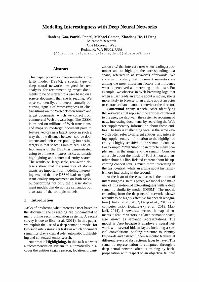
3.1 Network Architecture

The heart of the DSSM is a deep neural network

with convolutional structure, as shown in Figure

1. In what follows, we use lower-case bold letters,

such as 𝐱, to denote column vectors, 𝑥(𝑖) to de-

note the 𝑖𝑡ℎ element of 𝐱, and upper-case letters,

such as 𝐖, to denote matrices.

Input Layer 𝐱. It takes two steps to convert a doc-

ument 𝑑, which is a sequence of words, into a vec-

tor representation 𝐱 for the input layer of the net-

work: (1) convert each word in 𝑑 to a word vector,

and (2) build 𝐱 by concatenating these word vec-

tors. To convert a word 𝑤 into a word vector, we

first represent 𝑤 by a one-hot vector using a vo-

cabulary that contains 𝑁 high frequent words

(𝑁 = 150K in this study). Then, following Huang

et al. (2013), we map 𝑤 to a separate tri-letter vec-

tor. Consider the word “#dog#”, where # is a word

boundary symbol. The nonzero elements in its tri-

letter vector are “#do”, “dog”, and “og#”. We then

form the word vector of 𝑤 by concatenating its

one-hot vector and its tri-letter vector. It is worth

noting that the tri-letter vector complements the

one-hot vector representation in two aspects. First,

different OOV (out of vocabulary) words can be

represented by tri-letter vectors with few colli-

sions. Second, spelling variations of the same

word can be mapped to the points that are close to

each other in the tri-letter space. Although the

number of unique English words on the Web is

extremely large, the total number of distinct tri-

letters in English is limited (restricted to the most

frequent 30K in this study). As a result, incorpo-

rating tri-letter vectors substantially improves the

representation power of word vectors while keep-

ing their size small.

To form our input layer 𝐱 using word vectors,

we first identify a text span with a high degree of

relevance, called focus, in 𝑑 using task-specific

heuristics (see Sections 4 and 5 respectively). Sec-

ond, we form 𝐱 by concatenating each word vec-

tor in the focus and a vector that is the summation

of all other word vectors, as shown in Figure 1.

Since the length of the focus is much smaller than

that of its document, 𝐱 is able to capture the con-

textual information (for the words in the focus)

Web document into plain text, which is white-space to-

kenized and lowercased. Numbers are retained and no stem-

ming is performed. 2 We utilize the May 3, 2013 English Wikipedia dump con-

sisting of roughly 4.1 million articles from http://dumps.wiki-

media.org.

Figure 1: Illustration of the network architec-

ture and information flow of the DSSM

useful to the corresponding tasks, with a manage-

able vector size.

Convolutional Layer 𝐮 . A convolutional layer

extracts local features around each word 𝑤𝑖 in a

word sequence of length 𝐼 as follows. We first

generate a contextual vector 𝐜𝑖 by concatenating

the word vectors of 𝑤𝑖 and its surrounding words

defined by a window (the window size is set to 3

in this paper). Then, we generate for each word a

local feature vector 𝐮𝑖 using a tanh activation

function and a linear projection matrix 𝐖𝑐, which

is the same across all windows 𝑖 in the word se-

quence, as:

𝐮𝑖 = tanh(𝐖𝑐T𝐜𝑖) , where 𝑖 = 1 … 𝐼 (1)

Max-pooling Layer 𝐯. The size of the output 𝐮

depends on the number of words in the word se-

quence. Local feature vectors have to be com-

bined to obtain a global feature vector, with a

fixed size independent of the document length, in

order to apply subsequent standard affine layers.

We design 𝐯 by adopting the max operation over

each “time” 𝑖 of the sequence of vectors computed

by (1), which forces the network to retain only the

most useful, partially invariant local features pro-

duced by the convolutional layer:

𝑣(𝑗) = max𝑖=1,…,𝐼

{u𝑖(𝑗)} (2)

where the max operation is performed for each di-

mension of 𝐮 across 𝑖 = 1, … , 𝐼 respectively.

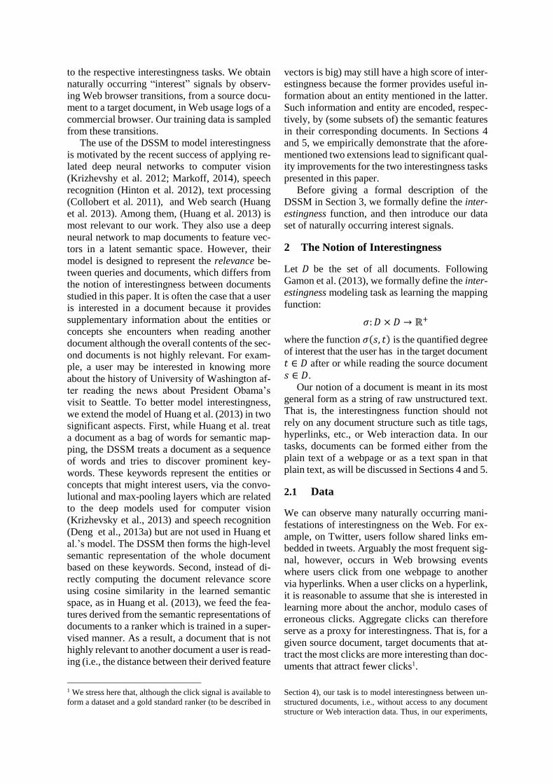
That convolutional and max-pooling layers are

able to discover prominent keywords of a docu-

ment can be demonstrated using the procedure in

Figure 2 using a toy example. First, the convolu-

tional layer of (1) generates for each word in a 5-

word document a 4-dimensional local feature vec-

tor, which represents a distribution of four topics.

For example, the most prominent topic of 𝑤2

within its three word context window is the first

topic, denoted by 𝑢2(1), and the most prominent

topic of 𝑤5 is 𝑢5(3). Second, we use max-pooling

of (2) to form a global feature vector, which rep-

resents the topic distribution of the whole docu-

ment. We see that 𝑣(1) and 𝑣(3) are two promi-

nent topics. Then, for each prominent topic, we

trace back to the local feature vector that survives

max-pooling:

𝑣(1) = max𝑖=1,…,5

{𝑢𝑖(1)} = 𝑢2(1)

𝑣(3) = max𝑖=1,…,5

{𝑢𝑖(3)} = 𝑢5(3).

Finally, we label the corresponding words of these

local feature vectors, 𝑤2 and 𝑤5, as keywords of

the document.

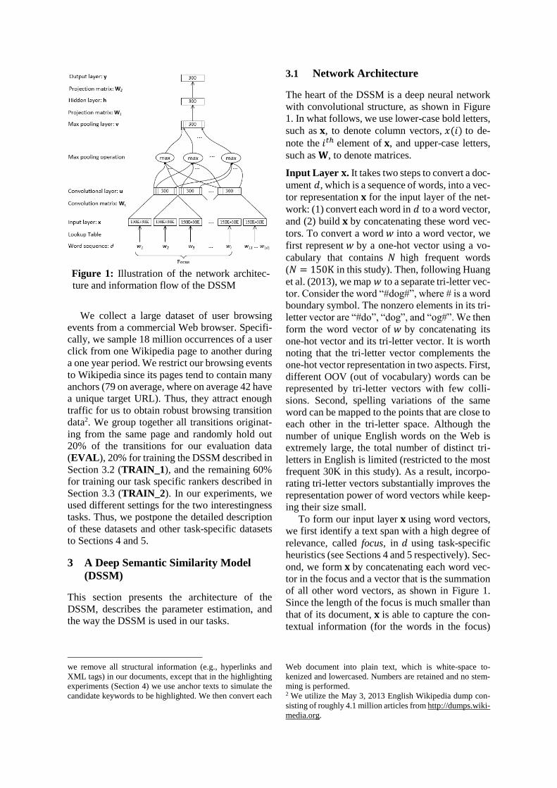
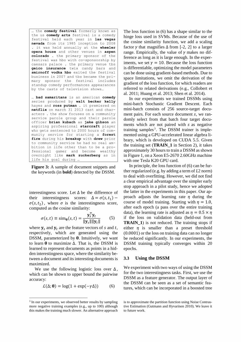
Figure 3 presents a sample of document snip-

pets and their keywords detected by the DSSM ac-

cording to the procedure elaborated in Figure 2. It

is interesting to see that many names are identified

as keywords although the DSSM is not designed

explicitly for named entity recognition.

Fully-Connected Layers 𝐡 and 𝐲 . The fixed

sized global feature vector 𝐯 of (2) is then fed to

several standard affine network layers, which are

stacked and interleaved with nonlinear activation

functions, to extract highly non-linear features 𝐲

at the output layer. In our model, shown in Figure

1, we have:

𝐡 = tanh(𝐖1T𝐯) (3)

𝐲 = tanh(𝐖2T𝐡) (4)

where 𝐖1 and 𝐖2 are learned linear projection matri-

ces.

3.2 Training the DSSM

To optimize the parameters of the DSSM of Fig-

ure 1, i.e., 𝛉 = {𝐖𝑐 , 𝐖1, 𝐖2}, we use a pair-wise

rank loss as objective (Yih et al. 2011). Consider

a source document 𝑠 and two candidate target

documents 𝑡1 and 𝑡2, where 𝑡1 is more interesting

than 𝑡2 to a user when reading 𝑠. We construct

two pairs of documents (𝑠, 𝑡1) and (𝑠, 𝑡2), where

the former is preferred and should have a higher

u1 u2 u3 u4 u5

w1 w2 w3 w4 w5

2

3

4

1

w1 w2 w3 w4 w5

v

2

3

4

1

Figure 2: Toy example of (upper) a 5-word

document and its local feature vectors ex-

tracted using a convolutional layer, and (bot-

tom) the global feature vector of the document

generated after max-pooling.

interestingness score. Let ∆ be the difference of

their interestingness scores: ∆ = 𝜎(𝑠, 𝑡1) −𝜎(𝑠, 𝑡2) , where 𝜎 is the interestingness score,

computed as the cosine similarity:

𝜎(𝑠, 𝑡) ≡ sim𝛉(𝑠, 𝑡) =𝐲𝑠

T𝐲𝑡

‖𝐲𝑠‖‖𝐲𝑡‖ (5)

where 𝐲𝑠 and 𝐲𝑡 are the feature vectors of 𝑠 and 𝑡,

respectively, which are generated using the

DSSM, parameterized by 𝛉. Intuitively, we want

to learn 𝛉 to maximize ∆. That is, the DSSM is

learned to represent documents as points in a hid-

den interestingness space, where the similarity be-

tween a document and its interesting documents is

maximized.

We use the following logistic loss over ∆ ,

which can be shown to upper bound the pairwise

accuracy:

ℒ(∆; 𝛉) = log(1 + exp(−𝛾∆)) (6)

3 In our experiments, we observed better results by sampling

more negative training examples (e.g., up to 100) although

this makes the training much slower. An alternative approach

The loss function in (6) has a shape similar to the

hinge loss used in SVMs. Because of the use of

the cosine similarity function, we add a scaling

factor 𝛾 that magnifies ∆ from [-2, 2] to a larger

range. Empirically, the value of 𝛾 makes no dif-

ference as long as it is large enough. In the exper-

iments, we set 𝛾 = 10. Because the loss function

is differentiable, optimizing the model parameters

can be done using gradient-based methods. Due to

space limitations, we omit the derivation of the

gradient of the loss function, for which readers are

referred to related derivations (e.g., Collobert et

al. 2011; Huang et al. 2013; Shen et al. 2014).

In our experiments we trained DSSMs using

mini-batch Stochastic Gradient Descent. Each

mini-batch consists of 256 source-target docu-

ment pairs. For each source document 𝑠, we ran-

domly select from that batch four target docu-

ments which are not paired with 𝑠 as negative

training samples3 . The DSSM trainer is imple-

mented using a GPU-accelerated linear algebra li-

brary, which is developed on CUDA 5.5. Given

the training set (TRAIN_1 in Section 2), it takes

approximately 30 hours to train a DSSM as shown

in Figure 1, on a Xeon E5-2670 2.60GHz machine

with one Tesla K20 GPU card.

In principle, the loss function of (6) can be fur-

ther regularized (e.g. by adding a term of 𝐿2 norm)

to deal with overfitting. However, we did not find

a clear empirical advantage over the simpler early

stop approach in a pilot study, hence we adopted

the latter in the experiments in this paper. Our ap-

proach adjusts the learning rate 𝜂 during the

course of model training. Starting with 𝜂 = 1.0,

after each epoch (a pass over the entire training

data), the learning rate is adjusted as 𝜂 = 0.5 × 𝜂

if the loss on validation data (held-out from

TRAIN_1) is not reduced. The training stops if

either 𝜂 is smaller than a preset threshold

(0.0001) or the loss on training data can no longer

be reduced significantly. In our experiments, the

DSSM training typically converges within 20

epochs.

3.3 Using the DSSM

We experiment with two ways of using the DSSM

for the two interestingness tasks. First, we use the

DSSM as a feature generator. The output layer of

the DSSM can be seen as a set of semantic fea-

tures, which can be incorporated in a boosted tree

is to approximate the partition function using Noise Contras-

tive Estimation (Gutmann and Hyvarinen 2010). We leave it

to future work.

… the comedy festival formerly known as

the us comedy arts festival is a comedy

festival held each year in las vegas

nevada from its 1985 inception to 2008

. it was held annually at the wheeler

opera house and other venues in aspen

colorado . the primary sponsor of the

festival was hbo with co-sponsorship by

caesars palace . the primary venue tbs

geico insurance twix candy bars and

smirnoff vodka hbo exited the festival

business in 2007 and tbs became the pri-

mary sponsor the festival includes

standup comedy performances appearances

by the casts of television shows…

… bad samaritans is an american comedy

series produced by walt becker kelly

hayes and ross putman . it premiered on

netflix on march 31 2013 cast and char-

acters . the show focuses on a community

service parole group and their parole

officer brian kubach as jake gibson an

aspiring professional starcraft player

who gets sentenced to 2000 hours of com-

munity service for starting a forest

fire during his breakup with drew prior

to community service he had no real am-

bition in life other than to be a pro-

fessional gamer and become wealthy

overnight like mark zuckerberg as in

life his goal during …

Figure 3: A sample of document snippets and

the keywords (in bold) detected by the DSSM.

based ranker (Friedman 1999) trained discrimina-

tively on the task-specific data. Given a source-

target document pair (𝑠, 𝑡), the DSSM generates

600 features (300 from the output layers 𝐲𝑠 and 𝐲𝑡

for each 𝑠 and 𝑡, respectively).

Second, we use the DSSM as a direct imple-

mentation of the interestingness function 𝜎. Re-

call from Section 3.2 that in model training, we

measure the interestingness score for a document

pair using the cosine similarity between their cor-

responding feature vectors (𝐲𝑠 and 𝐲𝑡). Similarly

at runtime, we define 𝜎 = sim𝛉(𝑠, 𝑡) as (5).

4 Experiments on Highlighting

Recall from Section 1 that in this task, a system

must select 𝑘 most interesting keywords in a doc-

ument that a user is reading. To evaluate our mod-

els using the click transition data described in Sec-

tion 2, we simulate the task as follows. We use the

set of anchors in a source document 𝑠 to simulate

the set of candidate keywords that may be of in-

terest to the user while reading 𝑠, and treat the text

of a document that is linked by an anchor in 𝑠 as a

target document 𝑡. As shown in Figure 1, to apply

DSSM to a specific task, we need to define the fo-

cus in source and target documents. In this task,

the focus in s is defined as the anchor text, and the

focus in t is defined as the first 10 tokens in t. We evaluate the performance of a highlighting

system against a gold standard interestingness

function 𝜎′ which scores the interestingness of an

anchor as the number of user clicks on 𝑡 from the

anchor in 𝑠 in our data. We consider the ideal se-

lection to then consist of the 𝑘 most interesting

anchors according to 𝜎′. A natural metric for this

task is Normalized Discounted Cumulative Gain

(NDCG) (Jarvelin and Kekalainen 2000).

We evaluate our models on the EVAL dataset

described in Section 2. We utilize the transition

distributions in EVAL to create three other test

sets, following the stratified sampling methodol-

ogy commonly employed in the IR community,

for the frequently, less frequently, and rarely

viewed source pages, referred to as HEAD,

TORSO, and TAIL, respectively. We obtain

these sets by first sorting the unique source docu-

ments according to their frequency of occurrence

in EVAL. We then partition the set so that HEAD

corresponds to all transitions from the source

pages at the top of the list that account for 20% of

the transitions in EVAL; TAIL corresponds to the

transitions at the bottom also accounting for 20%

of the transitions in EVAL; and TORSO corre-

sponds to the remaining transitions.

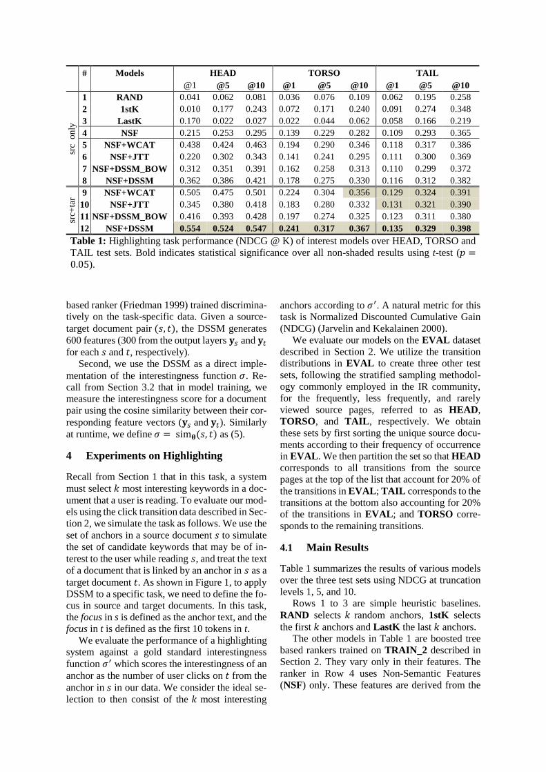
4.1 Main Results

Table 1 summarizes the results of various models

over the three test sets using NDCG at truncation

levels 1, 5, and 10.

Rows 1 to 3 are simple heuristic baselines.

RAND selects 𝑘 random anchors, 1stK selects

the first 𝑘 anchors and LastK the last 𝑘 anchors.

The other models in Table 1 are boosted tree

based rankers trained on TRAIN_2 described in

Section 2. They vary only in their features. The

ranker in Row 4 uses Non-Semantic Features

(NSF) only. These features are derived from the

# Models HEAD TORSO TAIL

@1 @5 @10 @1 @5 @10 @1 @5 @10

src

on

ly

1 RAND 0.041 0.062 0.081 0.036 0.076 0.109 0.062 0.195 0.258

2 1stK 0.010 0.177 0.243 0.072 0.171 0.240 0.091 0.274 0.348

3 LastK 0.170 0.022 0.027 0.022 0.044 0.062 0.058 0.166 0.219

4 NSF 0.215 0.253 0.295 0.139 0.229 0.282 0.109 0.293 0.365

5 NSF+WCAT 0.438 0.424 0.463 0.194 0.290 0.346 0.118 0.317 0.386

6 NSF+JTT 0.220 0.302 0.343 0.141 0.241 0.295 0.111 0.300 0.369

7 NSF+DSSM_BOW 0.312 0.351 0.391 0.162 0.258 0.313 0.110 0.299 0.372

8 NSF+DSSM 0.362 0.386 0.421 0.178 0.275 0.330 0.116 0.312 0.382

src+

tar

9 NSF+WCAT 0.505 0.475 0.501 0.224 0.304 0.356 0.129 0.324 0.391

10 NSF+JTT 0.345 0.380 0.418 0.183 0.280 0.332 0.131 0.321 0.390

11 NSF+DSSM_BOW 0.416 0.393 0.428 0.197 0.274 0.325 0.123 0.311 0.380

12 NSF+DSSM 0.554 0.524 0.547 0.241 0.317 0.367 0.135 0.329 0.398

Table 1: Highlighting task performance (NDCG @ K) of interest models over HEAD, TORSO and

TAIL test sets. Bold indicates statistical significance over all non-shaded results using t-test (𝑝 =0.05).

source document s and from user session infor-

mation in the browser log. The document features

include: position of the anchor in the document,

frequency of the anchor, and anchor density in the

paragraph.

The rankers in Rows 5 to 12 use the NSF and

the semantic features computed from source and

target documents of a browsing transition. We

compare semantic features derived from three dif-

ferent sources. The first feature source comes

from our DSSMs (DSSM and DSSM_BOW) us-

ing the output layers as feature generators as de-

scribed in Section 3.3. DSSM is the model de-

scribed in Section 3 and DSSM_BOW is the

model proposed by Huang et al. (2013) where

documents are view as bag of words (BOW) and

the convolutional and max-pooling layers are not

used. The two other sources of semantic features

are used as a point of comparison to the DSSM.

One is a generative semantic model (Joint Transi-

tion Topic model, or JTT) (Gamon et al. 2013).

JTT is an LDA-style model (Blei et al. 2003) that

is trained jointly on source and target documents

linked by browsing transitions. JTT generates a

total of 150 features from its latent variables, 50

each for the source topic model, the target topic

model and the transition model. The other seman-

tic model of contrast is a manually defined one,

which we use to assess the effectiveness of auto-

matically learned models against human model-

ers. To this effect, we use the page categories that

editors assign in Wikipedia as semantic features

(WCAT). These features number in the multiple

thousands. Using features such as WCAT is not a

viable solution in general since Wikipedia catego-

ries are not available for all documents. As such,

we use it solely as a point of comparison against

DSSM and JTT.

We also distinguish between two types of

learned rankers: those which draw their features

only from the source (src only) document and

those that draw their features from both the source

and target (src+tar) documents. Although our

task setting allows access to the content of both

source and target documents, there are practical

scenarios where a system should predict what in-

terests the user without looking at the target doc-

ument because the extra step of identifying a suit-

able target document for each candidate concept

or entity of interest is computationally expensive.

4.2 Analysis of Results

As shown in Table 1, NSF+DSSM, which incor-

porates our DSSM, is the overall best performing

system across test sets. The task is hard as evi-

denced by the weak baseline scores. One reason is

the large average number of candidates per page.

On HEAD, we found an average of 170 anchors

(of which 95 point to a unique target URL). For

TORSO and TAIL, we found the average number

of anchors to be 94 (52 unique targets) and 41 (19

unique targets), respectively.

Clearly, the semantics of the documents form

important signals for this task: WCAT, JTT,

DSSM_BOW, and DSSM all significantly boost

the performance over NSF alone. There are two

interesting comparisons to consider: (a) manual

semantics vs. learned semantics; and (b) deep se-

mantic models vs. generative topic models. On

(a), we observe somewhat surprisingly that the

learned DSSM produces features that outperform

the thousands of features coming from manually

(editor) assigned Wikipedia category features

(WCAT), in all but the TAIL where the two per-

form statistically the same. In contrast, features

from the generative model (JTT) perform worse

than WCAT across the board except on TAIL

where JTT and WCAT are statistically tied. On

(b), we observe that DSSM outperforms a state-

of-the-art generative model (JTT) on HEAD and

TORSO. On TAIL, they are statistically indistin-

guishable.

We turn now to inspecting the scenario where

features are only drawn from the source document

(Rows 1-8 in Table 1). Again we observe that se-

mantic features significantly boost the perfor-

mance against NSF alone, however they signifi-

cantly deteriorate when compared to using fea-

tures from both source and target documents. In

this scenario, the manual semantics from WCAT

outperform all other models, but with a diminish-

ing effect as we move from HEAD through

TORSO to TAIL. DSSM is the best performing

learned semantic model.

Finally, we present the results to justify the two

modifications we made to extend the model of

Huang et al. (2013) to the DSSM, as described in

Section 1. First, we see in Table 1 that

DSSM_BOW, which has the same network struc-

ture of Huang et al.’s model, is much weaker than

DSSM, demonstrating the benefits of using con-

volutional and max-pooling layers to extract se-

mantic features for the highlighting task. Second,

we conduct several experiments by using the co-

sine scores between the output layers of DSSM

for 𝑠 and 𝑡 as features (following the procedure in

Section 3.3 for using the DSSM as a direct imple-

mentation of 𝜎). We found that adding the cosine

features to NSF+DSSM does not lead to any im-

provement. We also combined NSF with solely

the cosine features from DSSM (i.e., without the

other semantic features drawn from its output lay-

ers). But we still found no improvement over us-

ing NSF alone. Thus, we conclude that for this

task it is much more effective to feed the features

derived from DSSM to a supervised ranker than

directly computing the interestingness score using

cosine similarity in the learned semantic space, as

in Huang et al. (2013).

5 Experiments on Entity Search

We construct the evaluation data set for this sec-

ond task by randomly sampling a set of documents

from a traffic-weighted set of Web documents. In

a second step, we identify the entity names in each

document using an in-house named entity recog-

nizer. We issue each entity name as a query to a

commercial search engine, and retain up to the

top-100 retrieved documents as candidate target

documents. We form for each entity a source doc-

ument which consists of the entity text and its sur-

rounding text defined by a 200-word window. We

define the focus (as in Figure 1) in 𝑠 as the entity

text, and the focus in 𝑡 as the first 10 tokens in 𝑡.

The final evaluation data set contains 10,000

source documents. On average, each source docu-

ment is associated with 87 target documents. Fi-

nally, the source-target document pairs are labeled

in terms of interestingness by paid annotators. The

label is on a 5-level scale, 0 to 4, with 4 meaning

the target document is the most interesting to the

source document and 0 meaning the target is of no

interest.

We test our models on two scenarios. The first

is a ranking scenario where 𝑘 interesting docu-

ments are displayed to the user. Here, we select

the top-𝑘 ranked documents according to their in-

terestingness scores. We measure the performance

via NDCG at truncation levels 1 and 3. The sec-

ond scenario is to display to the user all interesting

results. In this scenario, we select all target docu-

ments with an interestingness score exceeding a

predefined threshold. We evaluate this scenario

using ROC analysis and, specifically, the area un-

der the curve (AUC).

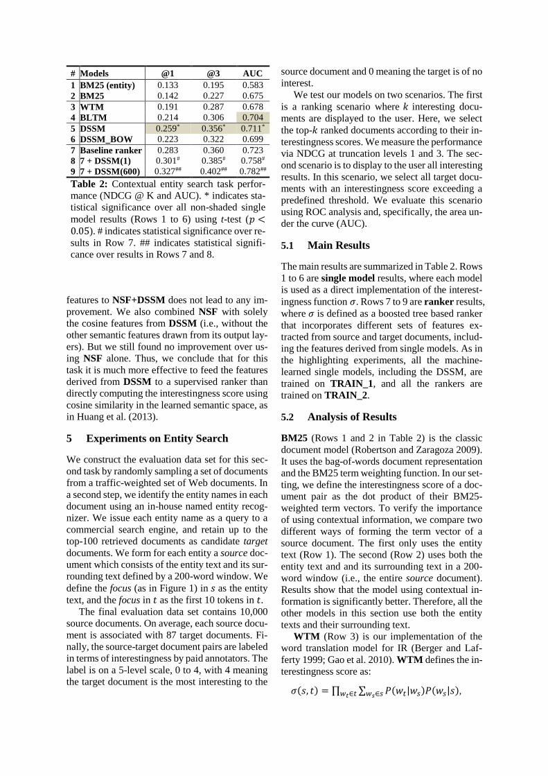
5.1 Main Results

The main results are summarized in Table 2. Rows

1 to 6 are single model results, where each model

is used as a direct implementation of the interest-

ingness function 𝜎. Rows 7 to 9 are ranker results,

where 𝜎 is defined as a boosted tree based ranker

that incorporates different sets of features ex-

tracted from source and target documents, includ-

ing the features derived from single models. As in

the highlighting experiments, all the machine-

learned single models, including the DSSM, are

trained on TRAIN_1, and all the rankers are

trained on TRAIN_2.

5.2 Analysis of Results

BM25 (Rows 1 and 2 in Table 2) is the classic

document model (Robertson and Zaragoza 2009).

It uses the bag-of-words document representation

and the BM25 term weighting function. In our set-

ting, we define the interestingness score of a doc-

ument pair as the dot product of their BM25-

weighted term vectors. To verify the importance

of using contextual information, we compare two

different ways of forming the term vector of a

source document. The first only uses the entity

text (Row 1). The second (Row 2) uses both the

entity text and and its surrounding text in a 200-

word window (i.e., the entire source document).

Results show that the model using contextual in-

formation is significantly better. Therefore, all the

other models in this section use both the entity

texts and their surrounding text.

WTM (Row 3) is our implementation of the

word translation model for IR (Berger and Laf-

ferty 1999; Gao et al. 2010). WTM defines the in-

terestingness score as:

𝜎(𝑠, 𝑡) = ∏ ∑ 𝑃(𝑤𝑡|𝑤𝑠)𝑃(𝑤𝑠|𝑠)𝑤𝑠∈𝑠𝑤𝑡∈𝑡 ,

# Models @1 @3 AUC

1 BM25 (entity) 0.133 0.195 0.583

2 BM25 0.142 0.227 0.675

3 WTM 0.191 0.287 0.678

4 BLTM 0.214 0.306 0.704

5 DSSM 0.259* 0.356* 0.711*

6 DSSM_BOW 0.223 0.322 0.699

7 Baseline ranker 0.283 0.360 0.723

8 7 + DSSM(1) 0.301# 0.385# 0.758#

9 7 + DSSM(600) 0.327## 0.402## 0.782##

Table 2: Contextual entity search task perfor-

mance (NDCG @ K and AUC). * indicates sta-

tistical significance over all non-shaded single

model results (Rows 1 to 6) using t-test (𝑝 <0.05). # indicates statistical significance over re-

sults in Row 7. ## indicates statistical signifi-

cance over results in Rows 7 and 8.

where 𝑃(𝑤𝑠|𝑠) is the unigram probability of word

𝑤𝑠 in 𝑠, and 𝑃(𝑤𝑡|𝑤𝑠) is the probability of trans-

lating 𝑤𝑠 into 𝑤𝑡, trained on source-target docu-

ment pairs using EM (Brown et al. 1993). The

translation-based approach allows any pair of

non-identical but semantically related words to

have a nonzero matching score. As a result, it sig-

nificantly outperforms BM25.

BTLM (Row 4) follows the best performing

bilingual topic model described in Gao et al.

(2011), which is an extension of PLSA (Hofmann

1999). The model is trained on source-target doc-

ument pairs using the EM algorithm with a con-

straint enforcing a source document 𝑠 and its tar-

get document 𝑡 to not only share the same prior

topic distribution, but to also have similar frac-

tions of words assigned to each topic. BLTM de-

fines the interestingness score between s and t as:

𝜎(𝑠, 𝑡) = ∏ ∑ 𝑃(𝑤𝑡|𝜙𝑧)𝑃(𝑧|𝜃𝑠)𝑧𝑤𝑡∈𝑡 .

The model assumes the following story of gener-

ating 𝑡 from 𝑠. First, for each topic 𝑧 a word dis-

tribution 𝜙𝑧 is selected from a Dirichlet prior with

concentration parameter 𝛽 . Second, given 𝑠 , a

topic distribution 𝜃𝑠 is drawn from a Dirichlet

prior with parameter 𝛼 . Finally, 𝑡 is generated

word by word. Each word 𝑤𝑡 is generated by first

selecting a topic 𝑧 according to 𝜃𝑠 , and then

drawing a word from 𝜙𝑧 . We see that BLTM

models interestingness by taking into account the

semantic topic distribution of the entire docu-

ments. Our results in Table 2 show that BLTM

outperforms WTM by a significant margin in

both NDCG and AUC.

DSSM (Row 5) outperforms all the competing

single models, including the state-of-the-art topic

model BLTM. Now, we inspect the difference be-

tween DSSM and BLTM in detail. Although both

models strive to generate the semantic representa-

tion of a document, they use different modeling

approaches. BLTM by nature is a generative

model. The semantic representation in BLTM is a

distribution of hidden semantic topics. Such a dis-

tribution is learned using Maximum Likelihood

Estimation in an unsupervised manner, i.e., max-

imizing the log-likelihood of the source-target

document pairs in the training data. On the other

hand, DSSM represents documents as points in a

hidden semantic space using a supervised learning

method, i.e., paired documents are closer in that

latent space than unpaired ones. We believe that

the superior performance of DSSM is largely due

to the fact that the model parameters are discrimi-

natively trained using an objective that is tailored

to the interestingness task.

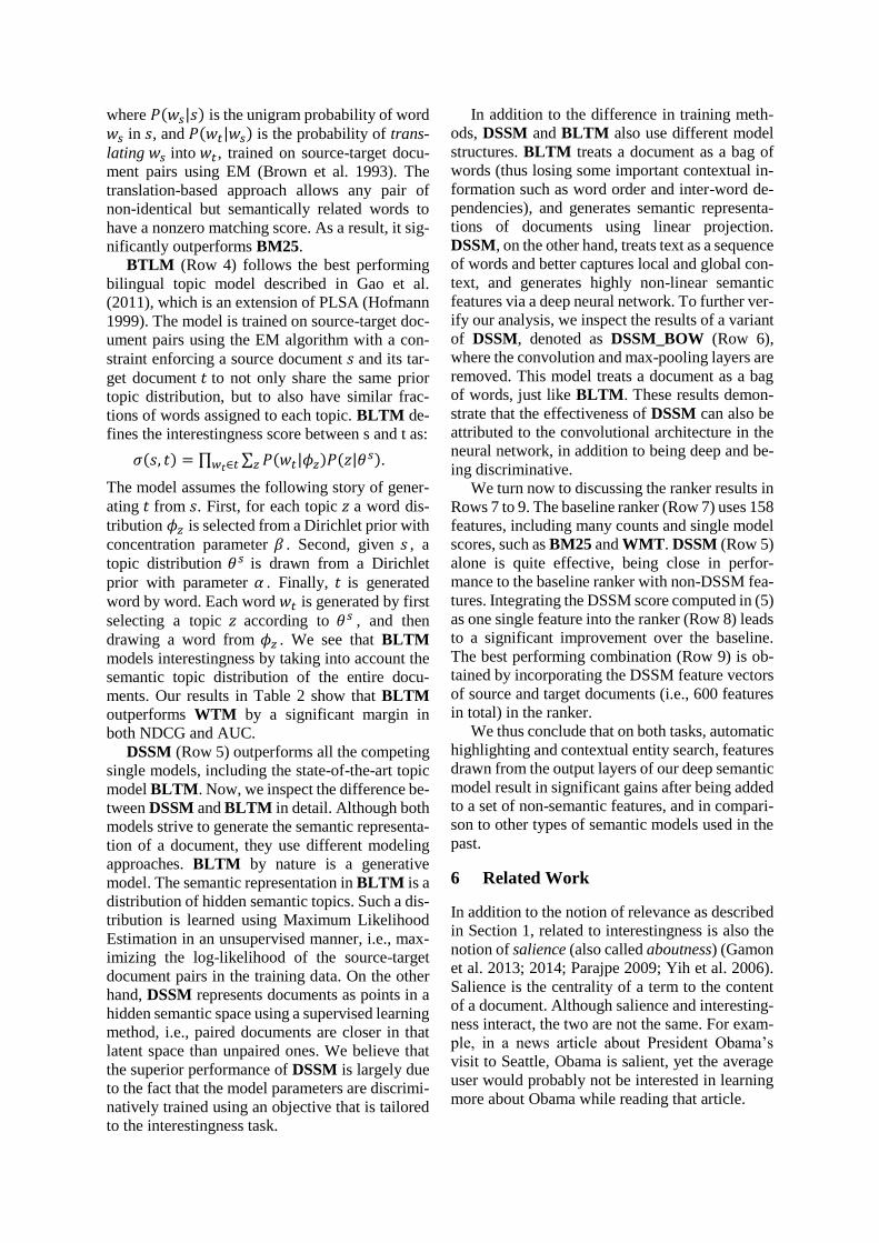
In addition to the difference in training meth-

ods, DSSM and BLTM also use different model

structures. BLTM treats a document as a bag of

words (thus losing some important contextual in-

formation such as word order and inter-word de-

pendencies), and generates semantic representa-

tions of documents using linear projection.

DSSM, on the other hand, treats text as a sequence

of words and better captures local and global con-

text, and generates highly non-linear semantic

features via a deep neural network. To further ver-

ify our analysis, we inspect the results of a variant

of DSSM, denoted as DSSM_BOW (Row 6),

where the convolution and max-pooling layers are

removed. This model treats a document as a bag

of words, just like BLTM. These results demon-

strate that the effectiveness of DSSM can also be

attributed to the convolutional architecture in the

neural network, in addition to being deep and be-

ing discriminative.

We turn now to discussing the ranker results in

Rows 7 to 9. The baseline ranker (Row 7) uses 158

features, including many counts and single model

scores, such as BM25 and WMT. DSSM (Row 5)

alone is quite effective, being close in perfor-

mance to the baseline ranker with non-DSSM fea-

tures. Integrating the DSSM score computed in (5)

as one single feature into the ranker (Row 8) leads

to a significant improvement over the baseline.

The best performing combination (Row 9) is ob-

tained by incorporating the DSSM feature vectors

of source and target documents (i.e., 600 features

in total) in the ranker. We thus conclude that on both tasks, automatic

highlighting and contextual entity search, features

drawn from the output layers of our deep semantic

model result in significant gains after being added

to a set of non-semantic features, and in compari-

son to other types of semantic models used in the

past.

6 Related Work

In addition to the notion of relevance as described

in Section 1, related to interestingness is also the

notion of salience (also called aboutness) (Gamon

et al. 2013; 2014; Parajpe 2009; Yih et al. 2006).

Salience is the centrality of a term to the content

of a document. Although salience and interesting-

ness interact, the two are not the same. For exam-

ple, in a news article about President Obama’s

visit to Seattle, Obama is salient, yet the average

user would probably not be interested in learning

more about Obama while reading that article.

There are many systems that identify popular

content in the Web or recommend content (e.g.,

Bandari et al. 2012; Lerman and Hogg 2010;

Szabo and Huberman 2010), which is closely re-

lated to the highlighting task. In contrast to these

approaches, we strive to predict what term a user

is likely to be interested in when reading content,

which may or may not be the same as the most

popular content that is related to the current docu-

ment. It has empirically been demonstrated in

Gamon et al. (2013) that popularity is in fact a ra-

ther poor predictor for interestingness. The task of

contextual entity search, which is formulated as an

information retrieval problem in this paper, is also

related to research on entity resolution (Stefanidis

et al. 2013).

Latent Semantic Analysis (Deerwester et al.

1990) is arguably the earliest semantic model de-

signed for IR. Generative topic models widely

used for IR include PLSA (Hofmann 1990) and

LDA (Blei et al. 2003). Recently, these models

have been extended to handle cross-lingual cases,

where there are pairs of corresponding documents

in different languages (e.g., Dumais et al. 1997;

Gao et al. 2011; Platt et al. 2010; Yih et al. 2011). By exploiting deep architectures, deep learning

techniques are able to automatically discover from

training data the hidden structures and the associ-

ated features at different levels of abstraction use-

ful for a variety of tasks (e.g., Collobert et al.

2011; Hinton et al. 2012; Socher et al. 2012;

Krizhevsky et al., 2012; Gao et al. 2014). Hinton

and Salakhutdinov (2010) propose the most origi-

nal approach based on an unsupervised version of

the deep neural network to discover the hierar-

chical semantic structure embedded in queries and

documents. Huang et al. (2013) significantly ex-

tends the approach so that the deep neural network

can be trained on large-scale query-document

pairs giving much better performance. The use of

the convolutional neural network for text pro-

cessing, central to our DSSM, was also described

in Collobert et al. (2011) and Shen et al. (2014)

but with very different applications. The DSSM

described in Section 3 can be viewed as a variant

of the deep neural network models used in these

previous studies.

7 Conclusions

Modeling interestingness is fundamental to many

online recommendation systems. We obtain natu-

rally occurring interest signals by observing Web

browsing transitions where users click from one

webpage to another. We propose to model this

“interestingness” with a deep semantic similarity

model (DSSM), based on deep neural networks

with special convolutional-pooling structure,

mapping source-target document pairs to feature

vectors in a latent semantic space. We train the

DSSM using browsing transitions between docu-

ments. Finally, we demonstrate the effectiveness

of our model on two interestingness tasks: auto-

matic highlighting and contextual entity search.

Our results on large-scale, real-world datasets

show that the semantics of documents computed

by the DSSM are important for modeling interest-

ingness and that the new model leads to signifi-

cant improvements on both tasks. DSSM is shown

to outperform not only the classic document mod-

els that do not use (latent) semantics but also state-

of-the-art topic models that do not have the deep

and convolutional architecture characterizing the

DSSM.

One area of future work is to extend our

method to model interestingness given an entire

user session, which consists of a sequence of

browsing events. We believe that the prior brows-

ing and interaction history recorded in the session

provides additional signals for predicting interest-

ingness. To capture such signals, our model needs

to be extended to adequately represent time series

(e.g., causal relations and consequences of ac-

tions). One potentially effective model for such a

purpose is based on the architecture of recurrent

neural networks (e.g., Mikolov et al. 2010; Chen

and Deng, 2014), which can be incorporated into

the deep semantic model proposed in this paper.

Additional Authors

Yelong Shen (Microsoft Research, One Microsoft

Way, Redmond, WA 98052, USA, email:

yeshen@microsoft.com).

Acknowledgments

The authors thank Johnson Apacible, Pradeep

Chilakamarri, Edward Guo, Bernhard Kohlmeier,

Xiaolong Li, Kevin Powell, Xinying Song and

Ye-Yi Wang for their guidance and valuable dis-

cussions. We also thank the three anonymous re-

viewers for their comments.

References

Bandari, R., Asur, S., and Huberman, B. A. 2012.

The pulse of news in social media: forecasting

popularity. In ICWSM.

Bengio, Y., 2009. Learning deep architectures for

AI. Fundamental Trends in Machine Learning,

2(1):1–127.

Berger, A., and Lafferty, J. 1999. Information re-

trieval as statistical translation. In SIGIR, pp.

222-229.

Blei, D. M., Ng, A. Y., and Jordan, M. J. 2003.

Latent Dirichlet allocation. Journal of Machine

Learning Research, 3.

Broder, A., Fontoura, M., Josifovski, V., and Riedel, L. 2007. A semantic approach to contex-tual advertising. In SIGIR.

Brown, P. F., Della Pietra, S. A., Della Pietra, V.

J., and Mercer, R. L. 1993. The mathematics of

statistical machine translation: parameter esti-

mation. Computational Linguistics, 19(2):263-

311.

Burges, C., Shaked, T., Renshaw, E., Lazier, A.,

Deeds, M., Hamilton, and Hullender, G. 2005.

Learning to rank using gradient descent. In

ICML, pp. 89-96.

Chen, J. and Deng, L. 2014. A primal-dual method

for training recurrent neural networks con-

strained by the echo-state property. In ICLR.

Collobert, R., Weston, J., Bottou, L., Karlen, M.,

Kavukcuoglu, K., and Kuksa, P., 2011. Natural

language processing (almost) from scratch.

Journal of Machine Learning Research, vol. 12.

Deerwester, S., Dumais, S. T., Furnas, G. W.,

Landauer, T., and Harshman, R. 1990. Indexing

by latent semantic analysis. Journal of the

American Society for Information Science,

41(6): 391-407

Deng, L., Hinton, G., and Kingsbury, B. 2013.

New types of deep neural network learning for

speech recognition and related applications: An

overview. In ICASSP.

Deng, L., Abdel-Hamid, O., and Yu, D., 2013a. A

deep convolutional neural network using heter-

ogeneous pooling for trading acoustic invari-

ance with phonetic confusion. In ICASSP.

Dumais, S. T., Letsche, T. A., Littman, M. L., and

Landauer, T. K. 1997. Automatic cross-linguis-

tic information retrieval using latent semantic

indexing. In AAAI-97 Spring Symposium Series:

Cross-Language Text and Speech Retrieval.

Friedman, J. H. 1999. Greedy function approxi-mation: a gradient boosting machine. Annals of Statistics, 29:1189-1232.

Gamon, M., Mukherjee, A., Pantel, P. 2014. Pre-dicting interesting things in text. In COLING.

Gamon, M., Yano, T., Song, X., Apacible, J. and Pantel, P. 2013. Identifying salient entities in web pages. In CIKM.

Gao, J., He, X., and Nie, J-Y. 2010. Clickthrough-

based translation models for web search: from

word models to phrase models. In CIKM. pp.

1139-1148.

Gao, J., He, X., Yih, W-t., and Deng, L. 2014.

Learning continuous phrase representations for

translation modeling. In ACL.

Gao, J., Toutanova, K., Yih., W-T. 2011. Click-

through-based latent semantic models for web

search. In SIGIR. pp. 675-684.

Graves, A., Mohamed, A., and Hinton, G. 2013.

Speech recognition with deep recurrent neural

networks. In ICASSP.

Gutmann, M. and Hyvarinen, A. 2010. Noise-con-trastive estimation: a new estimation principle for unnormalized statistical models. In Proc. Int. Conf. on Artificial Intelligence and Statis-tics (AISTATS2010).

Hinton, G., Deng, L., Yu, D., Dahl, G., Mohamed, A., Jaitly, N., Senior, A., Vanhoucke, V., Ngu-yen, P., Sainath, T., and Kingsbury, B., 2012. Deep neural networks for acoustic modeling in speech recognition. IEEE Signal Processing Magazine, 29:82-97.

Hinton, G., and Salakhutdinov, R., 2010. Discov-

ering binary codes for documents by learning

deep generative models. Topics in Cognitive

Science, pp. 1-18.

Hofmann, T. 1999. Probabilistic latent semantic

indexing. In SIGIR. pp. 50-57.

Huang, P., He, X., Gao, J., Deng, L., Acero, A.,

and Heck, L. 2013. Learning deep structured se-

mantic models for web search using click-

through data. In CIKM.

Jarvelin, K. and Kekalainen, J. 2000. IR evalua-

tion methods for retrieving highly relevant doc-

uments. In SIGIR. pp. 41-48.

Krizhevsky, A., Sutskever, I. and Hinton, G.

2012. ImageNet classification with deep convo-

lutional neural networks. In NIPS.

Lerman, K., and Hogg, T. 2010. Using a model of social dynamics to predict popularity of news. In WWW. pp. 621-630.

Markoff, J. 2014. Computer eyesight gets a lot more accurate. In New York Times.

Mikolov, T.. Karafiat, M., Burget, L., Cernocky, J., and Khudanpur, S. 2010. Recurrent neural network based language model. In INTERSPEECH. pp. 1045-1048.

Paranjpe, D. 2009. Learning document aboutness from implicit user feedback and document structure. In CIKM.

Platt, J., Toutanova, K., and Yih, W. 2010. Translingual document representations from discriminative projections. In EMNLP. pp. 251-261.

Ricci, F., Rokach, L., Shapira, B., and Kantor, P.

B. (eds) 2011. Recommender System Handbook,

Springer.

Robertson, S., and Zaragoza, H. 2009. The proba-

bilistic relevance framework: BM25 and be-

yond. Foundations and Trends in Information

Retrieval, 3(4):333-389.

Shen, Y., He, X., Gao. J., Deng, L., and Mesnil, G.

2014. A latent semantic model with convolu-

tional-pooling structure for information re-

trieval. In CIKM.

Socher, R., Huval, B., Manning, C., Ng, A., 2012.

Semantic compositionality through recursive

matrix-vector spaces. In EMNLP.

Stefanidis, K., Efthymiou, V., Herschel, M., and Christophides, V. 2013. Entity resolution in the web of data. CIKM’13 Tutorial.

Szabo, G., and Huberman, B. A. 2010. Predicting the popularity of online content. Communica-tions of the ACM, 53(8).

Wu, Q., Burges, C.J.C., Svore, K., and Gao, J. 2009. Adapting boosting for information re-trieval measures. Journal of Information Re-trieval, 13(3):254-270.

Yih, W., Goodman, J., and Carvalho, V. R. 2006. Finding advertising keywords on web pages. In WWW.

Yih, W., Toutanova, K., Platt, J., and Meek, C.

2011. Learning discriminative projections for

text similarity measures. In CoNLL.