Modeling cumulative effects of heavy metal contamination in mining areas of the Rimac basin

Lauren Butler

Advisor: Upmanu Lall

A thesis in partial fulfillment of the masters of science in Earth and Environmental Engineering

Columbia University, New York NY

2

ABSTRACT The Rimac river provides drinking water to Lima, the capital of Peru. Mines upstream release heavy metals into the river, but these can also be introduced by natural leaching, informal mining, and waste from previous mines. The effect of mining on water resources in Peru has instigated social conflict; identifying likely sources of contamination can suggest whether conflicts were related to real impacts or perceptions. This study models heavy metal concentrations using the mass of minerals produced by upstream mines to assess what contribution the mines make to downstream pollution. Historical water quality data from the Peruvian government was used, including concentrations of iron, cadmium, lead, chromium, copper, zinc, and manganese. These were measured twice monthly over seven years at 29 points in the Rimac basin. Time trends and spatial trends were analyzed for the whole basin using both percentiles of concentration, and ranked concentrations. Concentrations that exceeded Peruvian water quality standards were modeled with monthly flow and mine production data, using multiple linear regression, at three metallurgical and mining sites. The data was compared with key events such as conflict, mine closures, and regulation changes. Analysis showed that 100% of the metals studied exceeded the water quality standards every year. This increased with time, but the percentile analysis indicated that the time trend was not statistically significant. The spatial trend, however, showed markedly higher heavy metal presence at the upstream stations where the mining is concentrated, lower in the middle of the basin, and higher downstream where cumulative effects are more likely. The mine-level modeling showed that the factors correlated to concentration varied by site, but at no location did the model satisfactorily explain pollution variance using production and flow as predictors. No obvious effect was observed of regulation changes, except for decreased measurement frequency after political restructuring. The lack of time trend suggests that any cumulative effects are much larger in scale than the time period of this study, and the spatial trend indicates a possible distribution of effects. The consistent exceedance of ECAs indicates that environmental permitting, control or remediation within the Rimac basin are not yet sufficient. Models such as this one can help identify which mines, if any, most contribute to exceedance of a given metal at a given location. This will allow permitting, remediation, and source control to be done such that it considers local conditions and cumulative effects. KEY WORDS: Water quality, heavy metals, mining, cumulative effects, Peru

3

1. INTRODUCTION

1.1 EFFECTS OF HEAVY METALS IN WATER Below a certain threshold many heavy metals and transition metals are essential for human health (Hanikenne, 2009). But high doses are toxic, in part because metals bond to sulfur groups, interrupting cellular activity and contributing to oxidative damage. Negative health impacts of heavy metals have been observed in Peru (Ramos 2008). High levels of dissolved or colloidal metals are usually detrimental to the natural environment. They pose a risk to flora and fauna, especially to aquatic biota (Church, 2007), and the effects are compounded due to bioaccumulation. Heavy metals and low pH are known to be inversely correlated to plant growth, and the presence of heavy metals damages plant cell structures and inhibits enzymatic activity (Chibuike, 2014). The definition of heavy metals is not uniform in the current literature. Some have called for discontinued use of the term, others for a more pragmatic definition (Hubner, 2010). We take the second approach, and in this paper the term heavy metals includes the elements studied: iron, manganese, cadmium, copper, lead, zinc, and chromium.

1.2 CUMULATIVE EFFECTS Cumulative effects are commonly defined as “the impact on the environment which results from the incremental impact of the action when added to other past, present, and reasonably foreseeable future actions” (CEQ, 1999). Cumulative effects are especially important when considering heavy metals. Metals are a conservative contaminant, i.e. they are not readily transformed in a way that removes them from an ecosystem. In the mining industry, cumulative effects can be caused by space crowding, time crowding, interactions, or indirect effects (Kaveney, 2015). Considering cumulative effects is best supported by a catchment-based approach to water management (ICMM, 2015). Cumulative effects of any certain or reasonably foreseeable actions should be considered within Environmental Impact Assessments both in the U.S. and in Peru. There does not yet exist a standard method for their evaluation (ELAW, 2010), but best practices have been suggested (Solomon 2016, Kaveney 2015). Cumulative effects are not seen as a regulatory issue by the permitting agency of the Peruvian government (personal communication with Peruvian government official, Oct 2016). However, consideration of cumulative effective can only be effective if considered throughout the process, including the creation of laws and standards, impact assessment, permitting, fines, and regional environmental studies. Understanding water risk and accumulation of heavy metals not only protects the environment and human health, it also helps companies and governments know what is a sustainable investment. Water treatment and other infrastructure used to be 10% of mining companies’ infrastructure cost; now it's 30% (CDP, 2016). To make better use of all infrastructure, mines are increasingly located in clusters. The cumulative impacts of such arrangements are not well understood, and are become increasingly important.

4

1.3 WATER QUALITY MODELING Modeling heavy metals in water has often focused on the forms and sources of the metals at steady-state. Considering the different forms is important because ionic metals impact human health more than bound metals. Thermodynamic calculations can differentiate what percent of a total metal measurement is in each form, if the functional groups are known. Modelling programs that do this include MINEQL, MINTEQ, and PHREEQ. However, these are analyses at equilibrium conditions and do not consider changes over time. They would not be appropriate for a study of cumulative effects. Furthermore, water chemistry and mineral pollution is complex beyond current understanding when considered in a real, basin-level ecosystem. A statistical approach as taken in this study will lose some of the details such as differentiating functional forms of each metal, but allows for a bigger picture understanding. The concentrations of metals used in this study are of total metals. SPARROW is a hybrid statistical and physical process model developed by the USGS for basin-level modelling of water quality. It has been primarily used for nutrient levels, and has not yet been used for heavy metals. Although the data availability in Rimac would be sufficient to run a SPARROW model, SPARROW is a steady-state analysis. It assumes that the release of contaminants, from riverbed deposition for example, is in equilibrium with immobilization of the same contaminants (Schwarz, 2006). Including a time component would mean that more complex and shorter time scale processes would also need to be considered if incorporating physical processes in the model. Such processes are not yet well enough understood for a model. Therefore, a purely statistical approach is taken in this study, though an understanding of the physical processes and the SPARROW model design have informed the approach. As discussed in further detail below, the short time span of data relative to mining history in this case, and lack of time trends observed, indicate that a SPARROW-like model could have also been appropriate. Many models exist for heavy metal concentration in soils (Buszewski 2006, Badaoui 2011), but modeling is less common in surface water. According to the Peruvian National Water Authority, this is the first study of mineral transport in surface water in Peru (personal communication, 2016). A mathematical system model was developed for arsenic in river in Romania (Crivineanu, 2012), and metal concentration was predicted for surface water in Iran using neural network and multiple linear regression models (Rooki, 2011).

1.4 WATER AND MINING IN PERU Mineral commodities account for 60% of Peru's exports, primarily gold, copper, and zinc. (EY, 2014). Peru is South America’s most water-stressed country and every year mining and metallurgy release over 13 billion m3 of effluents into Peru’s water courses (Bebbington, 2008). The Tyndall Centre for Climate Change Research identifies Peru as the world’s third most

Commented [LB1]: Make automatic numbering, as Header style

5

vulnerable country to the impacts of climate change. Connections between mining and water risks are many. There is competition over water availability. In Southern Peru, water tables are reported to be declining and entire lakes have been depleted for use in mining (personal communication with mining industry personnel, 2016). Mining development is limited to locations where a reliable water source can be secured, sometimes resulting in stranded assets. Elsewhere, mining projects previously approved by the government have been cancelled due to the expectation of water competition between agriculture and mining, for example in Tambogrande (Markham, 2003). It is also notable that water resources in Peru can become a point of collaboration, not only competition. However, places where water availability has improved as a result of synergistic development and responsible mining operation pass largely unnoticed and undocumented.

In addition to water quantity impacts, changes to water quality are a major effect of mining in Peru. Contamination from mining affects population centers, which are concentrated to the west of the Andes, as well as fragile ecosystems to the west. Active mines, closed or abandoned mines, informal mining, natural leaching, agriculture and other industries often affect water quality in the same basin. Regulation and monitoring was non-existent when mining first was established in Peru, resulting in environmental risks from over 6,000 legacy sites today (K-Water, 2015).

1.5 REGULATORY AND SOCIAL CONTEXT Levels of heavy metals in surface water in Peru are governed by the Environmental code of 1990 with regulatory updates by the Ministry of Environment for mining effluents in 1996 and for water bodies in 2008 (Llontop 2010). Effluents from mines are regulated by Maximum Permissible Limits (MPL). The effluents mix with surface water which is regulated via Standards of Environmental Quality (ECAs for the name in Spanish). Exceedance of MPLs can be fined, as can discharge without a permit and established MPLs, but there are no sanctions regarding ECAs unless causality can be proven. Ideally, the MPLs for each mine in an area would be determined such that if all are being met, the ECAs are also maintained. For this, an understanding of cumulative effects would be necessary. But MPLs might not be adequate even in isolation. They are determined within Environmental Impact Assessments (EIA). The agency that approved these documents, previously within the Department of Energy and Mines, had limited capacity to challenge the claims and reports prepared by mining companies. Rather than predicting amounts of heavy metals released, the EIAs commonly cite the regulations that pertain to specific bodies of water and make an assurance that the mine will pollute only within those limits. When a mine’s discharge surpasses their MPL, fees may be symbolic or forgiven. The agency responsible for fines, OEFA, saw its power decreased with Article 19 of Law 30230. This is popularly known as the paquetazo ambiental, meaning “environmental package” that has burdensome consequences.

6

The perceived unfairness or ineffectiveness of these processes create a lack of trust by local communities. This exacerbates social conflict over mining's effect on water resources (Slack, 2013) and often slows or halts extraction. This has occurred at the mines Tia Maria, Las Bambas, La Zanja, Conga, Antamina, Yanacocha and others in Cajamarca and Piura. Both the impacts of a mine on critical water resources and the perception of impacts are factors in social unrest (ICMM, 2012). Indeed, communities upstream of mines have reported pollution, indicating that “mining is associated with contamination through perception as well as reality” (Budds, 2015). Environmental Impact Assessments which consider cumulative effects would improve neighboring communities’ trust that all impacts are being considered (Slack, 2013). Over the last decade progress has been made toward improving regulation, reporting, and monitoring on a project basis. This includes updated Environmental Quality Standards in 2008 (Llontop, 2010) and 2015, and a requirement for citizen involvement and monitoring. It is usually nominal, but at least 30 communities are actively monitoring water quality (UNDP, 2016). The recent developments may improve understanding and reduction of negative project impacts. However, still very little is measured or understood about the impacts of multiple mining projects and contamination sources.

1.6 RIMAC BASIN

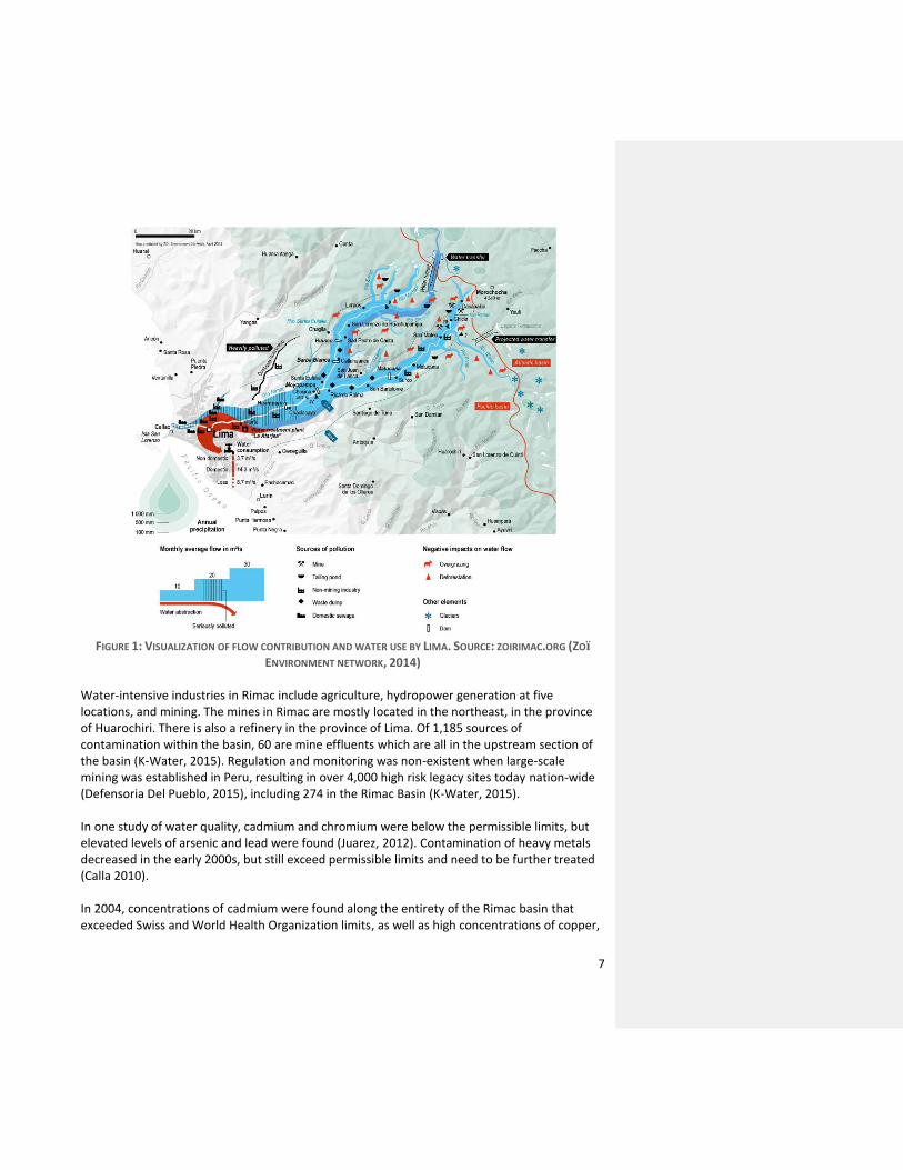
The Rimac River starts at over 5,000 meters of elevation in the Andes mountain range and has three main tributaries: Blanco, Aruri, and Huaycoloro as shown in Figure 1. It then goes to the La Atarjea treatment plant before entering Lima, the capital of Peru. The Rimac river supplies most of the drinking water in Lima. Water-related risks in the Rimac basin include debris flow and diminishing glaciers which replenish water supply. Earthquakes are common, and there are tailing dams near seismic faults (personal communication with National Water Authority, 2016).

7

FIGURE 1: VISUALIZATION OF FLOW CONTRIBUTION AND WATER USE BY LIMA. SOURCE: ZOIRIMAC.ORG (ZO��

ENVIRONMENT NETWORK, 2014)

Water-intensive industries in Rimac include agriculture, hydropower generation at five locations, and mining. The mines in Rimac are mostly located in the northeast, in the province of Huarochiri. There is also a refinery in the province of Lima. Of 1,185 sources of contamination within the basin, 60 are mine effluents which are all in the upstream section of the basin (K-Water, 2015). Regulation and monitoring was non-existent when large-scale mining was established in Peru, resulting in over 4,000 high risk legacy sites today nation-wide (Defensoria Del Pueblo, 2015), including 274 in the Rimac Basin (K-Water, 2015). In one study of water quality, cadmium and chromium were below the permissible limits, but elevated levels of arsenic and lead were found (Juarez, 2012). Contamination of heavy metals decreased in the early 2000s, but still exceed permissible limits and need to be further treated (Calla 2010). In 2004, concentrations of cadmium were found along the entirety of the Rimac basin that exceeded Swiss and World Health Organization limits, as well as high concentrations of copper,

8

lead, zinc and arsenic at many locations. The high levels of cadmium may be caused by mining both directly and indirectly. Processing of sphalerite and pyrite found in the region forms sulfuric acid, which facilitates leaching of minerals such as cadmium present in the natural geology. All but arsenic were considered attributable to mining based on the geochemistry of the region and the mining activity. At the time of the study only arsenic exceeded the legal limits (Méndez, 2005), but the Peruvian water quality standards have been since updated. In the San Mateo district of Rimac, exceedances of cadmium, lead, manganese, arsenic and iron motivated a suggestion for improved treatment of the effluent of nearby mining company San Juan S.A. (Llontop, 2010), though no direct link was shown. Heavy metals in streambed sediments also exceeded limits in Rimac and the two adjacent basins (Rivera, 2007).

2. METHODS

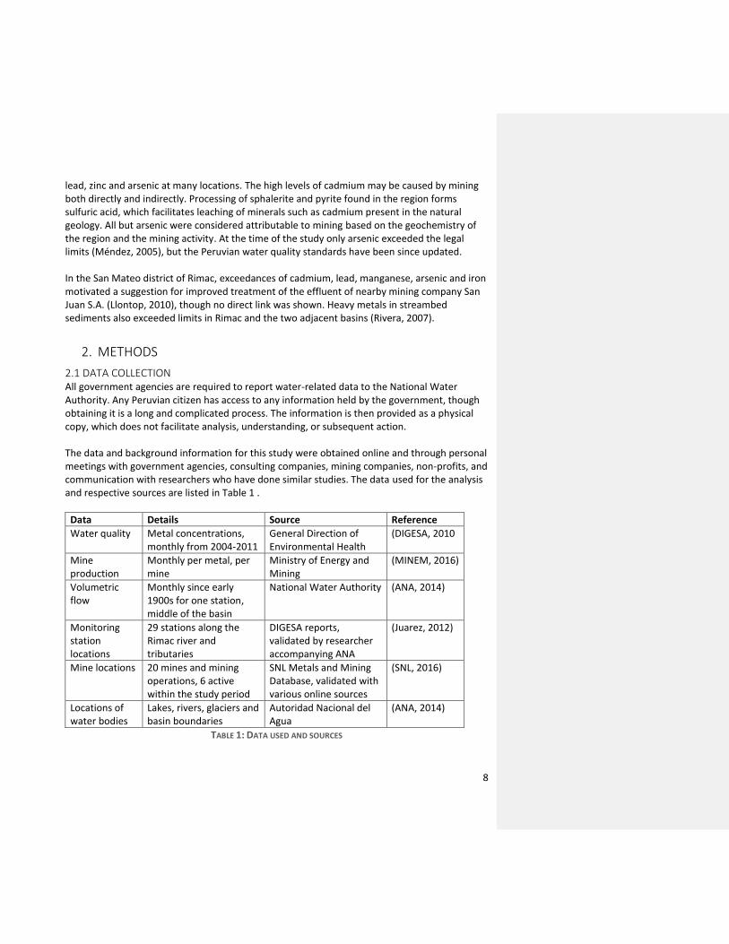
2.1 DATA COLLECTION All government agencies are required to report water-related data to the National Water Authority. Any Peruvian citizen has access to any information held by the government, though obtaining it is a long and complicated process. The information is then provided as a physical copy, which does not facilitate analysis, understanding, or subsequent action. The data and background information for this study were obtained online and through personal meetings with government agencies, consulting companies, mining companies, non-profits, and communication with researchers who have done similar studies. The data used for the analysis and respective sources are listed in Table 1 .

Data Details Source Reference

Water quality Metal concentrations, monthly from 2004-2011

General Direction of Environmental Health

(DIGESA, 2010

Mine production

Monthly per metal, per mine

Ministry of Energy and Mining

(MINEM, 2016)

Volumetric flow

Monthly since early 1900s for one station, middle of the basin

National Water Authority (ANA, 2014)

Monitoring station locations

29 stations along the Rimac river and tributaries

DIGESA reports, validated by researcher accompanying ANA

(Juarez, 2012)

Mine locations 20 mines and mining operations, 6 active within the study period

SNL Metals and Mining Database, validated with various online sources

(SNL, 2016)

Locations of water bodies

Lakes, rivers, glaciers and basin boundaries

Autoridad Nacional del Agua

(ANA, 2014)

TABLE 1: DATA USED AND SOURCES

9

There are potential issues with the water quality data. A community organizer and resident of Chosica, a town in the middle of Rimac, shared the perception that National Water Authority chooses to take samples where they know it is least likely to be contaminated- for example, far from the mining operations (personal communication, 2016). Officially, all sampling is done according to a planned experimental design, with consistent locations. For the data we used, two of the years provided geographic coordinates for the collection of the samples, of which only one varied significantly (by about 0.5km), indicating that the locations for this data were fairly consistent. However, another government agency mentioned changing the location of monitoring due to excavation that was being done just upstream of the monitoring station (personal communication, 2016), to avoid undue influence of sediment from the contaminating event on the sample. It is possible that true contamination is higher than the available data, due to attempts to avoid sampling in the most contaminated areas. In addition, mining companies are reported to know when the government agencies are going to come to take water samples, so they could preemptively shut down some of the operations on that day. Data that were not obtained for this study, and represent potential gaps in the analysis, include: (1) flow data for each point of the basin studied, and (2) locations of informal mining hubs and estimates of their production. The data collection was done during trips to Lima in May 2016 and October 2016. Interviews were held with over 60 stakeholders to understand the local context and complexities that affect water quality in mining regions. Meetings were held with government agencies, non-profits, community members, environmental monitoring committees, universities, and mining companies.

2.2 SITE SELECTION Based on recommendations made in the interviews mentioned above, the Rimac basin was chosen due to the environmental degradation, data availability, long history with mining, and importance to decision makers in Lima. Understanding contamination in the Rimac basin was identified as especially vital because it becomes drinking water for the eight million people in Lima. A trip along the entirety of the Rimac River and part of the Blanco River enabled verification of the geographical data obtained and status of mines. The geographically referenced data was mapped using ArcMAP, RStudio, and Google Earth. The distribution within the basin of water resources, mining areas, legacy sites, monitoring locations, and main towns were analyzed. Key areas were chosen where multiple water quality stations and mines or mineral processing was active during the time period of the study. For each of the areas chosen, events such as mine closures, openings, sales, and social conflict were identified by reviewing historical Peruvian news sources and mining investment news. The volumetric flow data used was at the middle of basin, in Chosica. The flow is not the same throughout the basin, but the cycles and trends at Chosica are expected to be representative of

10

other locations. There is more precipitation at higher elevations in the Rimac basin, but all rivers within the basin have similar annual cycles (Mendéz, 2005). Flow at other places along the river can be approximated with scaling factors.

2.3 NETWORK DEVELOPMENT To understand cumulative effects, complete development of a cause-effect network “which defines the interconnections for the web of effects” is critical (Solomon, 2016). We created a network for Rimac, excluding mines that were not active during the study period and monitoring stations that had little or no data. We identified points in the network that could be modeled on a regional level, i.e. a monitoring station that had a major mine or mineral processing plant immediately upstream and another monitoring station upstream of the mine. For each time 𝑡 where there is a reading of water quality, concentration 𝐶 of contaminant 𝑐 is provided at a given location (longitude 𝑥, latitude 𝑦, and elevation 𝑧). This is assigned to the nearest station 𝑠, even in cases when the exact 𝑥, 𝑦, 𝑧 values vary between years. Likewise, production 𝑃 is summed where the mine locations 𝑥, 𝑦, 𝑧 is within a small diameter 𝛿 of a central location 𝑥∗, 𝑦∗, and owned by the same parent company, thereby designated as being within ball 𝛽: this is called mine location 𝑙.

𝑷𝒎,𝒕,𝒍 = 𝑷𝒎,𝒕,𝒙,𝒚,𝒛 | (𝒙, 𝒚) 𝝐 𝜷(𝒙∗, 𝒚∗, 𝜹) 𝑪𝒔,𝒕,𝒄 = 𝑪𝒕,𝒄,𝒙,𝒚,𝒛 | (𝒙, 𝒚) 𝝐 𝜷(𝒙∗, 𝒚∗, 𝜹) EQUATION 1

Thus, two- or three-dimensional spatial relationships are reduced to a subset of linear structures where causal effects can be modelled. Where the spatial arrangement from upstream to downstream is 𝑠𝑖 → 𝑙 → 𝑠𝑖+1, the model dependencies are as follows, such that downstream concentration is influenced by the concentration upstream of the mine and the production of the mine or mining cluster.

𝒇(𝑪 𝒔𝒊+𝟏,𝒕,𝒄 | 𝑪 𝒔𝒊,𝒕,𝒄 , 𝑷𝒎,𝒕,𝒍 ) EQUATION 2

Three regions were identified with water quality readings both upstream and downstream of a mines or mine operations, where the mine was also classified as medium or large by the data provider MINEM and there were at least 12 months of production during the study period.

2.4 PRODUCTION For each region, we normalized the production of each metal. The normalized production for metal 𝑚, time 𝑡, and mining location 𝑙, is the production 𝑃 divided by the summed production over all active months of the mine. For mines that were active during the entire study period, total months 𝑇= 84 = 12 months × 7 years. As discussed above, the minimum acceptable value for T is 12.

11

��𝒎,𝒕,𝒍 = 𝑻 ∗𝑷𝒎,𝒕,𝒍

∑ 𝑷𝒎,𝒍𝑻𝒕=𝟏

EQUATION 3

The production data was reported in varying units (grams for gold, kg for silver, and metric tons for the rest), so normalization allowed for plotting all metals together without losing the relative importance of gold and silver production. In addition to normalizing the production data, a rank and sum method was used. Each original reading was replaced with a value relative to where it falls within the population of readings. This method allows a comparison of metals that have very different ranges and units, and reduces the undue influence of outliers. The ranks were summed over all mines to give a single time series representing the basin-wide production. This was then used as a predictor for models as described in section 2.7.

2.5 WATER QUALITY Water quality data from 2004 to 2016 was compiled from four Peruvian government agencies- the General Direction of Health (DIGESA), the National Water Authority (ANA), Lima’s Drinking Water and Sewer Service (SEDAPAL), the Organism of Evaluation and Environmental Oversight (OEFA), as well as other short-term monitoring by community groups, non-profits, and academics (Méndez 2005, Llontop 2010). Comparisons showed that the DIGESA data was more frequently and regularly recorded than any of the other sources, so it alone was used in the data analysis. The data available in this consistent and complete format ended in 2010. The reports provided many water quality parameters, but we used only heavy metals. While sulfates and pH may be informative in mining areas, they can also be affected by other industries. Heavy metals in the Rimac basin are most likely introduced by natural geochemistry or mining. We chose a subset of seven metals based on the completeness of the data available. For most measurements, month and year were provided but not the date or time. All measurements were assigned a decimal time at the midpoint of each month. Concentrations below the detection limit (DL) of the measurement technique had been reported as DL, <DL, or 0. There were also NA values which were assumed to be distinct, representing non-completion of a test. The detection limit varied by metal and changed during the study period presumably due to improving measurement techniques, creating multiply censored data. We compiled a database across all stations and determined the detection limit for each metal as the lowest reading excluding 0 values, which were likely inconsistent reporting and were considered the same as <DL. We converted all 0, DL, and <DL values to DL.

𝑪𝒔,𝒕,𝒄 = {𝑪𝒔,𝒕,𝒄 , 𝑪𝒔,𝒕,𝒄 > 𝑫𝑳

𝑫𝑳 , 𝑪𝒔,𝒕,𝒄 ≤ 𝑫𝑳 EQUATION 4

12

There were many missing values; over sixty percent of the expected results were reported as NA or left blank. To complete the data we used multiple imputation by chained equations, with five imputations using predictive mean matching. To compare between metals, the value of interest is not concentration but rather how much a concentration exceeds the water quality standard (ECA) for a given metal contaminant 𝑐. The exceedance ratio 𝐸 for each time and station was calculated according to Equation 1.

𝑬𝒔,𝒕,𝒄 =𝑪𝒔,𝒕,𝒄 (

𝒎𝒈

𝑳)

𝑬𝑪𝑨𝒄 (𝒎𝒈

𝑳) EQUATION 5

The legal limits 𝐸𝐶𝐴 varied for each metal, and were obtained from a DIGESA water quality report. The ECAs are determined by the classification of each water body. The Rimac River, upstream of Lima’s water treatment plant, is categorized as "Category 1": superficial waters destined to produce drinking water. The sub-category "A2" indicates that it can be made potable with conventional treatment as opposed to simply disinfection or more advanced treatment (DIGESA, 2010). In addition to using exceedance ratios, the original data were ranked. This statistical method replaces an original reading with a value relative to where it falls within the population of readings. Like converting to exceedances, it allows a comparison of metals that have very different ranges. Ranking was chosen because it also reduces the undue influence of outliers. The ranked matrix was then subjected to a quantile analysis. For each percentile 𝑖, a new matrix was created with binary values depending on whether the concentration at a given station,

month, and contaminant exceeded the 𝑖𝑡ℎ percentile of all data for that contaminant. An aggregate exposure index 𝐼 was then computed by summing this binary exceedance index over the seven metals, for each sampling date at each station.

𝒒𝒔,𝒕,𝒄,𝒊 = {𝟎 , 𝑪𝒔,𝒕,𝒄 ≤ 𝑸𝒊

𝟏 , 𝑪𝒔,𝒕,𝒄 > 𝑸𝒊 EQUATION 6

𝑰𝒔,𝒕,𝒊 = 𝒒𝒔,𝒕,𝑪𝒅,𝒊 + 𝒒𝒔,𝒕,𝑪𝒖,𝒊 + 𝒒𝒔,𝒕,𝑪𝒓,𝒊 + 𝒒𝒔,𝒕,𝑷𝒃,𝒊 + 𝒒𝒔,𝒕,𝒁𝒏,𝒊 + 𝒒𝒔,𝒕,𝑴𝒏,𝒊 + 𝒒𝒔,𝒕,𝑭𝒆,𝒊 EQUATION 7

Where 𝑖 = {50, 90, 99, 95}. This resulted in a single number per time period, per station, that was used for trend identification. Finally, a binary matrix was created similar to the process above, based on whether a result exceeded the ECA. A value of 1 was assigned for exceeding and a 0 for within the water quality standards. Then we summed the exceedances across metals to get a single time trend and simplified spatial trends.

2.6 EXPLORATORY ANALYSIS

13

The distribution and trends of data were analyzed using Mann Kendall tests, seasonal Mann Kendall, and local regressions. Similar tests were done for each station, and for each metal. All coding tests, and models were completed in RStudio. Trends were analyzed for the whole basin, each mining location, and for the downstream stations right before Lima. The normalized production of each metal for a given mine was plotted over time; this helped identify abrupt changes that may correspond to social conflict, changes in regulation, or changes in mine ownership or operation. The metal exceedances over time were graphed with the time trends of mine production, to visually identify correlations between water quality and mine production. This was also done quantitatively using correlation matrices for each area. Principle components were used to analyze the data, and showed that the first principle component explained most of the variance. Thus, it was appropriate to use just one component in the modelling. Also used were histograms of data distribution and larceny, Q-Q plots, analysis of variance, and correlation matrices.

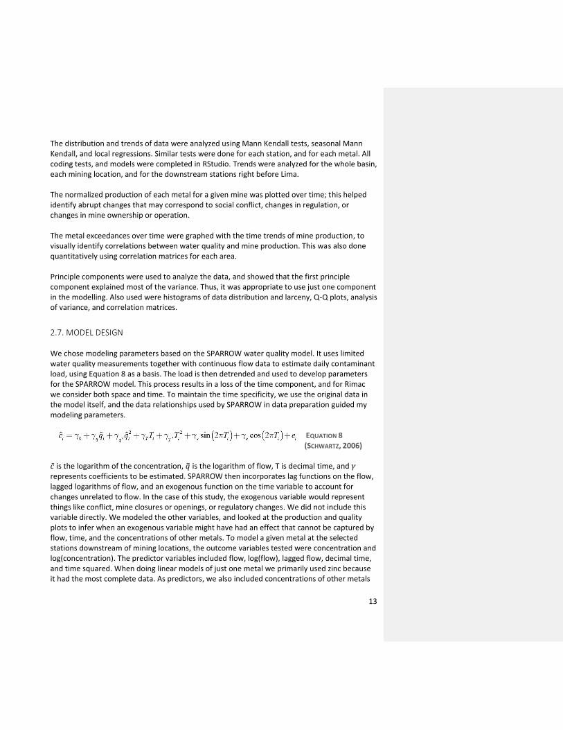
2.7. MODEL DESIGN We chose modeling parameters based on the SPARROW water quality model. It uses limited water quality measurements together with continuous flow data to estimate daily contaminant load, using Equation 8 as a basis. The load is then detrended and used to develop parameters for the SPARROW model. This process results in a loss of the time component, and for Rimac we consider both space and time. To maintain the time specificity, we use the original data in the model itself, and the data relationships used by SPARROW in data preparation guided my modeling parameters.

EQUATION 8

(SCHWARTZ, 2006) �� is the logarithm of the concentration, �� is the logarithm of flow, T is decimal time, and 𝛾 represents coefficients to be estimated. SPARROW then incorporates lag functions on the flow, lagged logarithms of flow, and an exogenous function on the time variable to account for changes unrelated to flow. In the case of this study, the exogenous variable would represent things like conflict, mine closures or openings, or regulatory changes. We did not include this variable directly. We modeled the other variables, and looked at the production and quality plots to infer when an exogenous variable might have had an effect that cannot be captured by flow, time, and the concentrations of other metals. To model a given metal at the selected stations downstream of mining locations, the outcome variables tested were concentration and log(concentration). The predictor variables included flow, log(flow), lagged flow, decimal time, and time squared. When doing linear models of just one metal we primarily used zinc because it had the most complete data. As predictors, we also included concentrations of other metals

14

at the same station, concentrations of the same metal at upstream stations, and logarithms thereof. We did not include the cyclical time terms in Equation 8, but they could be included in future iterations. To study basin-wide effects, variety of models were tested with water quality as the outcome variable. This was done using linear models and local regressions. We modelled the first principle component of water quality for the whole basin with flow as the predictor variable, and did the same for the farthest downstream stations. Then, the PC of the farthest upstream station was added as a predictor, as was flow. Finally, the time series produced by each quantile analysis was modeled with the summed production rank time series. There are many processes that affect heavy metal concentration downstream that are not directly considered here. For example, a full hydrologic model would identify elevation changes and dams where metal-laden sediment would accumulate and be released under flood conditions. All local conditions must be considered when doing a deterministic model. In this study, a fully stochastic approach is taken which captures local conditions by looking at historical correlations. We also exclude production data for hydrocarbon and other non-metallic extraction, which are present in Rimac.

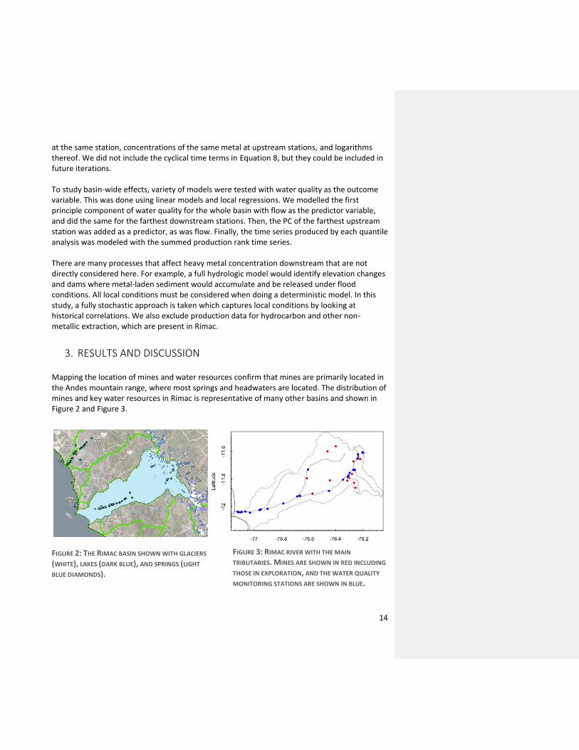
3. RESULTS AND DISCUSSION Mapping the location of mines and water resources confirm that mines are primarily located in the Andes mountain range, where most springs and headwaters are located. The distribution of mines and key water resources in Rimac is representative of many other basins and shown in Figure 2 and Figure 3.

FIGURE 2: THE RIMAC BASIN SHOWN WITH GLACIERS

(WHITE), LAKES (DARK BLUE), AND SPRINGS (LIGHT

BLUE DIAMONDS).

FIGURE 3: RIMAC RIVER WITH THE MAIN

TRIBUTARIES. MINES ARE SHOWN IN RED INCLUDING

THOSE IN EXPLORATION, AND THE WATER QUALITY

MONITORING STATIONS ARE SHOWN IN BLUE.

15

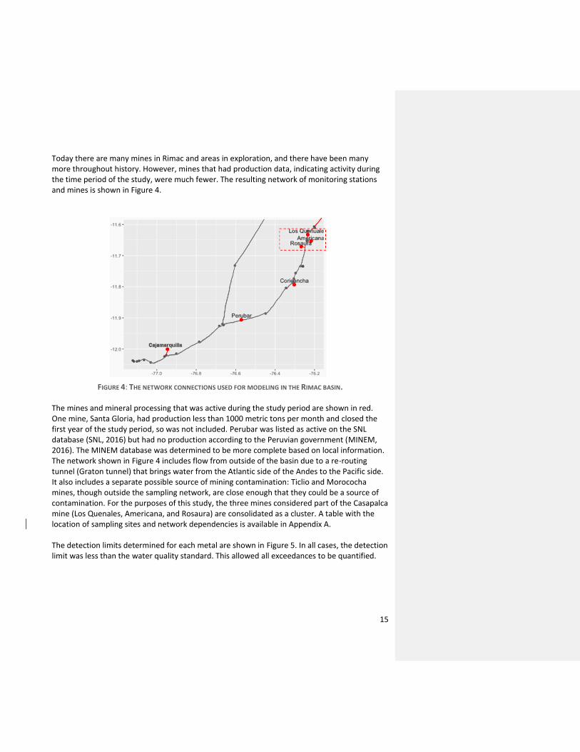
Today there are many mines in Rimac and areas in exploration, and there have been many more throughout history. However, mines that had production data, indicating activity during the time period of the study, were much fewer. The resulting network of monitoring stations and mines is shown in Figure 4.

FIGURE 4: THE NETWORK CONNECTIONS USED FOR MODELING IN THE RIMAC BASIN.

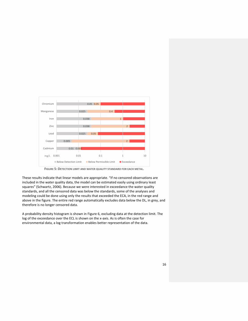
The mines and mineral processing that was active during the study period are shown in red. One mine, Santa Gloria, had production less than 1000 metric tons per month and closed the first year of the study period, so was not included. Perubar was listed as active on the SNL database (SNL, 2016) but had no production according to the Peruvian government (MINEM, 2016). The MINEM database was determined to be more complete based on local information. The network shown in Figure 4 includes flow from outside of the basin due to a re-routing tunnel (Graton tunnel) that brings water from the Atlantic side of the Andes to the Pacific side. It also includes a separate possible source of mining contamination: Ticlio and Morococha mines, though outside the sampling network, are close enough that they could be a source of contamination. For the purposes of this study, the three mines considered part of the Casapalca mine (Los Quenales, Americana, and Rosaura) are consolidated as a cluster. A table with the location of sampling sites and network dependencies is available in Appendix A. The detection limits determined for each metal are shown in Figure 5. In all cases, the detection limit was less than the water quality standard. This allowed all exceedances to be quantified.

16

FIGURE 5: DETECTION LIMIT AND WATER QUALITY STANDARD FOR EACH METAL.

These results indicate that linear models are appropriate. “If no censored observations are included in the water quality data, the model can be estimated easily using ordinary least squares” (Schwartz, 2006). Because we were interested in exceedance the water quality standards, and all the censored data was below the standards, some of the analyses and modeling could be done using only the results that exceeded the ECA, in the red range and above in the figure. The entire red range automatically excludes data below the DL, in grey, and therefore is no longer censored data. A probability density histogram is shown in Figure 6, excluding data at the detection limit. The log of the exceedance over the ECL is shown on the x-axis. As is often the case for environmental data, a log transformation enables better representation of the data.

0.01

0.005

0.025

0.038

0.038

0.025

0.05

0.003

2

0.05

2

1

0.4

0.05

0.001 0.01 0.1 1 10

Cadmium

Copper

Lead

Zinc

Iron

Manganese

Chromium

Below Detection Limit Below Permissible Limit Exceedance

mg/L

17

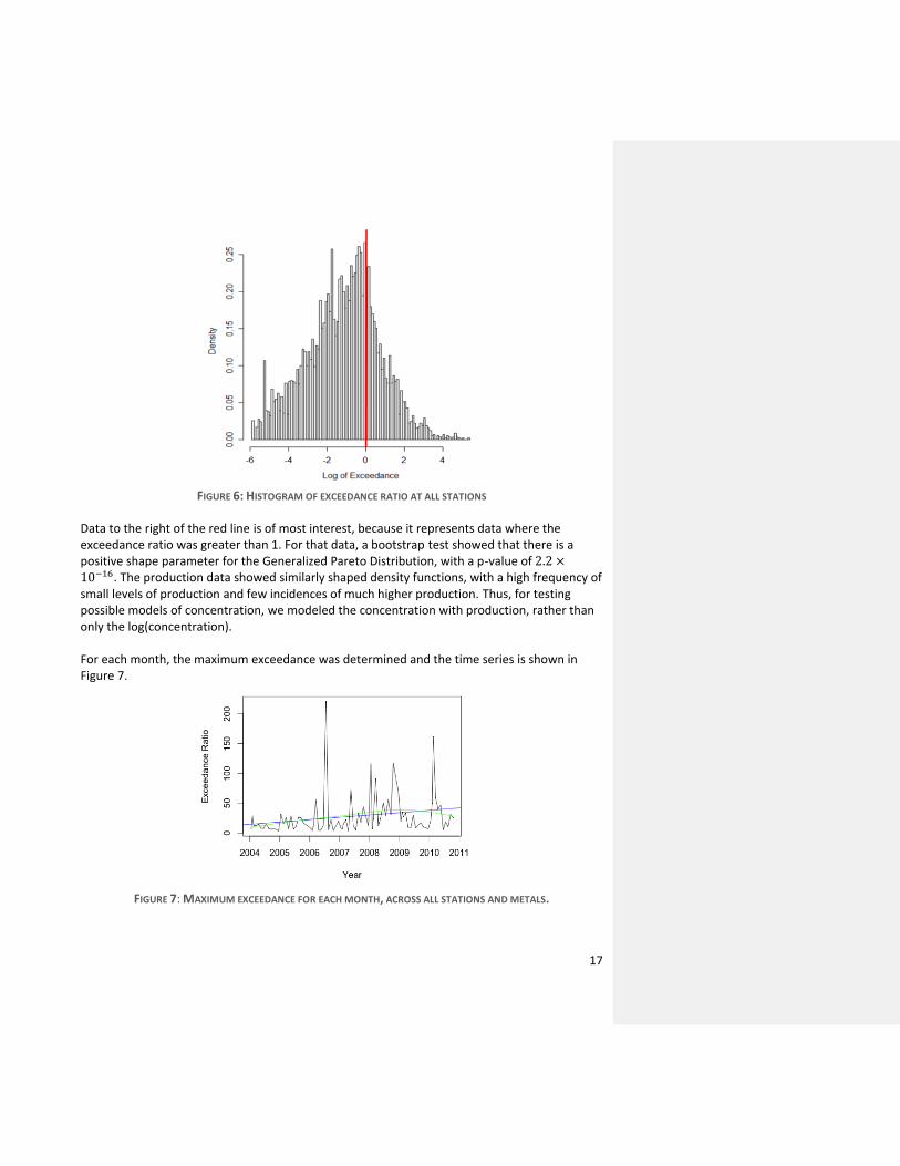
FIGURE 6: HISTOGRAM OF EXCEEDANCE RATIO AT ALL STATIONS

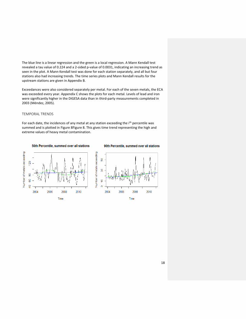
Data to the right of the red line is of most interest, because it represents data where the exceedance ratio was greater than 1. For that data, a bootstrap test showed that there is a positive shape parameter for the Generalized Pareto Distribution, with a p-value of 2.2 ×10−16. The production data showed similarly shaped density functions, with a high frequency of small levels of production and few incidences of much higher production. Thus, for testing possible models of concentration, we modeled the concentration with production, rather than only the log(concentration). For each month, the maximum exceedance was determined and the time series is shown in Figure 7.

FIGURE 7: MAXIMUM EXCEEDANCE FOR EACH MONTH, ACROSS ALL STATIONS AND METALS.

18

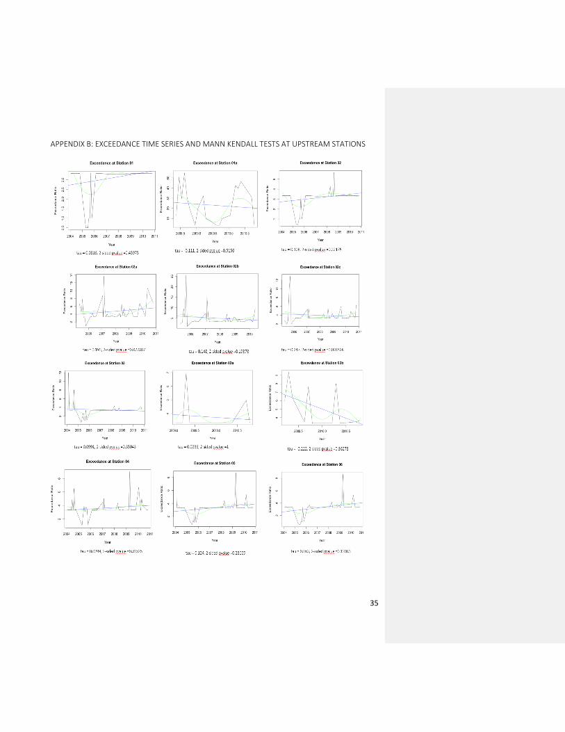
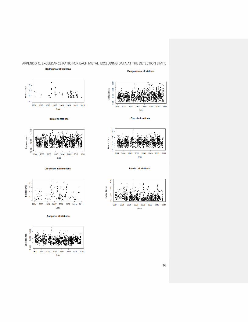
The blue line is a linear regression and the green is a local regression. A Mann Kendall test revealed a tau value of 0.224 and a 2-sided p-value of 0.0031, indicating an increasing trend as seen in the plot. A Mann Kendall test was done for each station separately, and all but four stations also had increasing trends. The time series plots and Mann Kendall results for the upstream stations are given in Appendix B. Exceedances were also considered separately per metal. For each of the seven metals, the ECA was exceeded every year. Appendix C shows the plots for each metal. Levels of lead and iron were significantly higher in the DIGESA data than in third-party measurements completed in 2003 (Méndez, 2005).

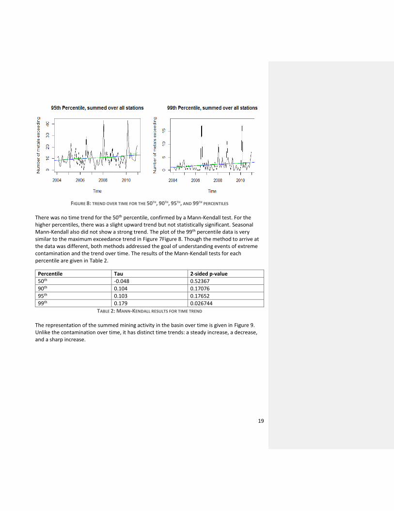
TEMPORAL TRENDS For each date, the incidences of any metal at any station exceeding the ith percentile was summed and is plotted in Figure 8Figure 8. This gives time trend representing the high and extreme values of heavy metal contamination.

19

FIGURE 8: TREND OVER TIME FOR THE 50TH, 90TH, 95TH, AND 99TH PERCENTILES

There was no time trend for the 50th percentile, confirmed by a Mann-Kendall test. For the higher percentiles, there was a slight upward trend but not statistically significant. Seasonal Mann-Kendall also did not show a strong trend. The plot of the 99th percentile data is very similar to the maximum exceedance trend in Figure 7Figure 8. Though the method to arrive at the data was different, both methods addressed the goal of understanding events of extreme contamination and the trend over time. The results of the Mann-Kendall tests for each percentile are given in Table 2.

Percentile Tau 2-sided p-value

50th -0.048 0.52367

90th 0.104 0.17076

95th 0.103 0.17652

99th 0.179 0.026744

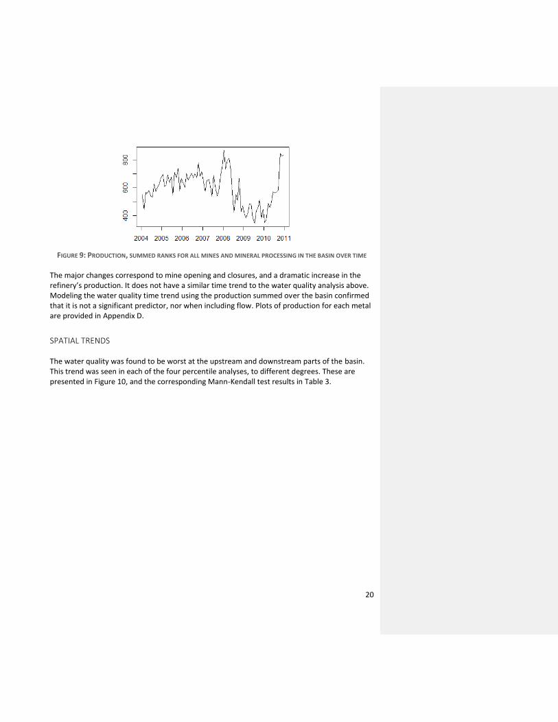
TABLE 2: MANN-KENDALL RESULTS FOR TIME TREND The representation of the summed mining activity in the basin over time is given in Figure 9. Unlike the contamination over time, it has distinct time trends: a steady increase, a decrease, and a sharp increase.

20

FIGURE 9: PRODUCTION, SUMMED RANKS FOR ALL MINES AND MINERAL PROCESSING IN THE BASIN OVER TIME

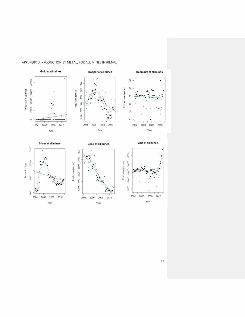
The major changes correspond to mine opening and closures, and a dramatic increase in the refinery’s production. It does not have a similar time trend to the water quality analysis above. Modeling the water quality time trend using the production summed over the basin confirmed that it is not a significant predictor, nor when including flow. Plots of production for each metal are provided in Appendix D.

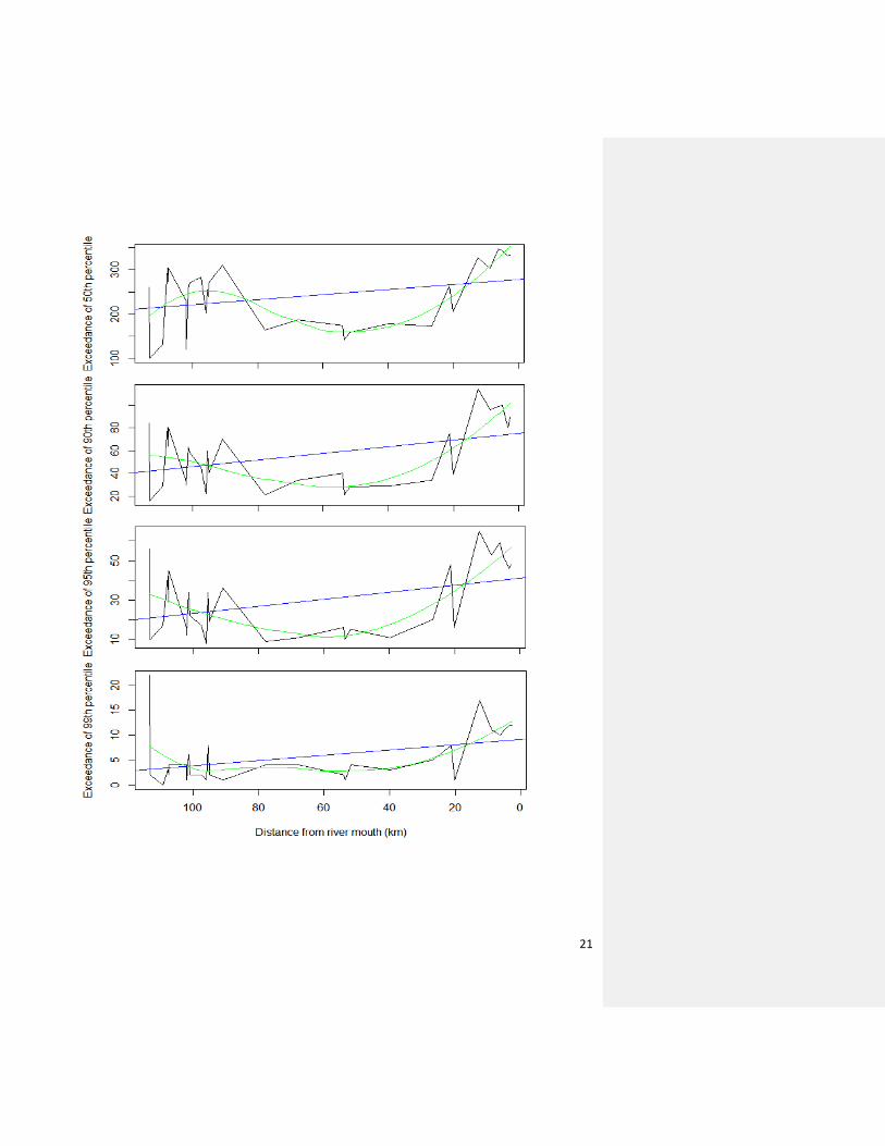
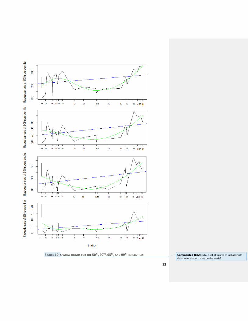
SPATIAL TRENDS The water quality was found to be worst at the upstream and downstream parts of the basin. This trend was seen in each of the four percentile analyses, to different degrees. These are presented in Figure 10, and the corresponding Mann-Kendall test results in Table 3.

21

22

FIGURE 10: SPATIAL TRENDS FOR THE 50TH, 90TH, 95TH, AND 99TH PERCENTILES Commented [LB2]: which set of figures to include: with distance or station name on the x-axis?

23

Percentile Tau 2-sided p-value 50th 0.222 0.082894

90th 0.173 0.17905

95th 0.163 0.20792

99th 0.342 0.0095655

TABLE 3: MANN-KENDALL RESULTS FOR SPATIAL TREND GOING DOWNSTREAM An upward trend is present in all percentiles, but it is most pronounced in the 99th percentile. The graphs show that the overall trend is upwards, but the more descriptive pattern is a U-shape; the highest presence of heavy metals is in the upstream and downstream sections, and lower in the middle of the basin. It is expected that heavy metal concentrations would be higher at the upstream monitoring locations, due to the presence of more mines there. The mining in Peru happens mostly along the Andes mountain range, and the Rimac basin is no exception. The mineral-rich area has historic and active mines, and it’s possible there is more natural leaching in the highlands than in the downstream locations. The increase in contamination at the downstream locations is a possible indicator of cumulative effects. As the Rimac river reaches the flatter area from Chosica to Lima and into the ocean, heavy metals would have more time to settle to the riverbed. Storms and other disturbances could then dislodge the stored metals, causing high readings as seen in this analysis. Though spatial flow data was not used in this analysis, it is known that the middle of the basin is where flow rate is the highest in the Rimac River. This can be seen graphically in Figure 1. The water quality data used is concentration of heavy metals. Therefore, the addition or extraction of water quantity will affect the reading of heavy metals. It is possible that the overall metal mass is consistent over space, but the addition of water from tributaries causes the concentration to drop in the middle of the basin. Then after station 18, most of the river water is extracted at the La Atarjea drinking water plant, treated, and distributed to the city. It is possible that this extraction affects the heavy metal concentration data used in this study, for stations 19-23 which are downstream of the treatment plant. However, it is unlikely that drinking water extraction provides a full explanation for the downstream increase in heavy metals. First, the observations of increased contamination begin at station E16, which is upstream of the plant. Second, the plant extracts the water as is, and is not expected to change the quality. If they were instead extracting, treating for metals, and returning the metals to the river’s diminished quantity of flow, that would have a significant effect on the concentration. But the La Atarjea plant does not treat for heavy metals; the heavy metals observed in this study upstream of La Atarjea are distributed for human consumption throughout Lima. Therefore, it is likely that flow volume and cumulative effects both influence the spatial trends in heavy metal concentration. Spatially distributed flow data would be necessary to differentiate the relative contribution of the two factors.

24

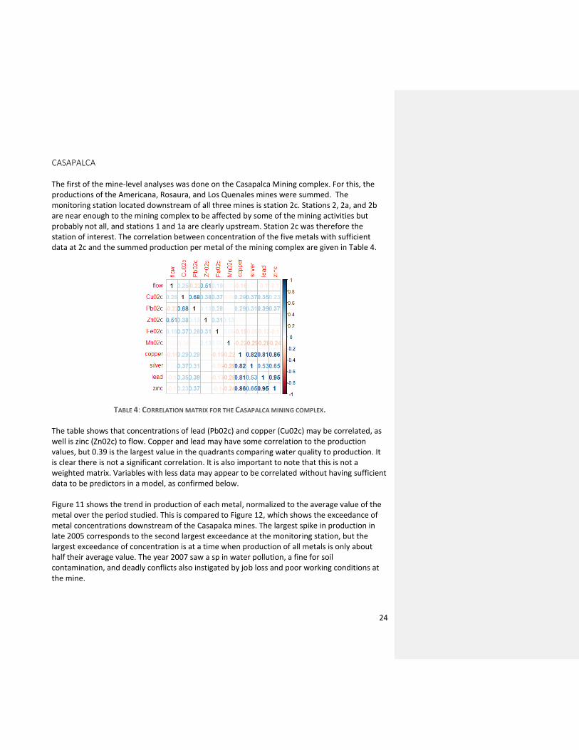
CASAPALCA The first of the mine-level analyses was done on the Casapalca Mining complex. For this, the productions of the Americana, Rosaura, and Los Quenales mines were summed. The monitoring station located downstream of all three mines is station 2c. Stations 2, 2a, and 2b are near enough to the mining complex to be affected by some of the mining activities but probably not all, and stations 1 and 1a are clearly upstream. Station 2c was therefore the station of interest. The correlation between concentration of the five metals with sufficient data at 2c and the summed production per metal of the mining complex are given in Table 4.

TABLE 4: CORRELATION MATRIX FOR THE CASAPALCA MINING COMPLEX.

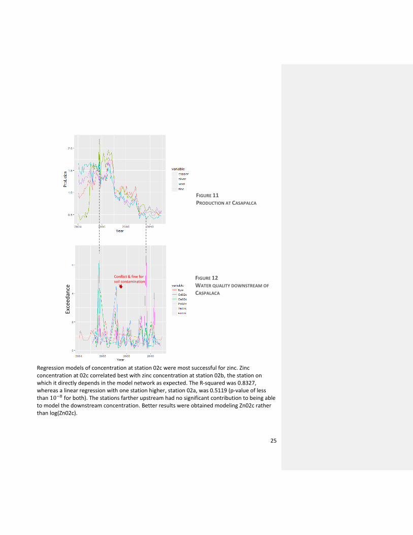
The table shows that concentrations of lead (Pb02c) and copper (Cu02c) may be correlated, as well is zinc (Zn02c) to flow. Copper and lead may have some correlation to the production values, but 0.39 is the largest value in the quadrants comparing water quality to production. It is clear there is not a significant correlation. It is also important to note that this is not a weighted matrix. Variables with less data may appear to be correlated without having sufficient data to be predictors in a model, as confirmed below. Figure 11 shows the trend in production of each metal, normalized to the average value of the metal over the period studied. This is compared to Figure 12, which shows the exceedance of metal concentrations downstream of the Casapalca mines. The largest spike in production in late 2005 corresponds to the second largest exceedance at the monitoring station, but the largest exceedance of concentration is at a time when production of all metals is only about half their average value. The year 2007 saw a sp in water pollution, a fine for soil contamination, and deadly conflicts also instigated by job loss and poor working conditions at the mine.

25

FIGURE 11 PRODUCTION AT CASAPALCA

FIGURE 12 WATER QUALITY DOWNSTREAM OF

CASPALACA Regression models of concentration at station 02c were most successful for zinc. Zinc concentration at 02c correlated best with zinc concentration at station 02b, the station on which it directly depends in the model network as expected. The R-squared was 0.8327, whereas a linear regression with one station higher, station 02a, was 0.5119 (p-value of less than 10−8 for both). The stations farther upstream had no significant contribution to being able to model the downstream concentration. Better results were obtained modeling Zn02c rather than log(Zn02c).

Exce

edan

ce

ee

Conflict & fine for soil contamination

26

The variance of manganese concentrations could be explained in part by zinc concentrations, but only with an adjusted R-squared of 0.5781. For most metals, such a result was the best obtained, indicating that the heavy metal concentration at station 02c is influenced in large part by factors not considered here. In summary, Station 02c depends on 02b, somewhat on 02a, and minimally on flow. The production at Casapalca mine did not explain variance or trends in the downstream concentration of any metals. It is possible that the contamination in this area is more related to historical cumulative effects from well before the period of this study. There are many tailings dams in the area that have accumulated over previous decades (Schwarz, 2010). Comparison with concurrent events shows that operations were suspended at Rosaura in 2008, in part responsible for a decrease in overall production (Biznews, 2010). There was deadly conflict in 2007, mostly over lost jobs and poor working conditions. Contamination of soils resulted in fines for Casapalca in June of the same year (Agua, 2007). While the conflicts were not directly due to water quality, it is possible that the contamination of soil was related to the third largest peak in metal concentration in Figure 12. If this was the case, the spike in water contamination may have been able to act as an early warning.

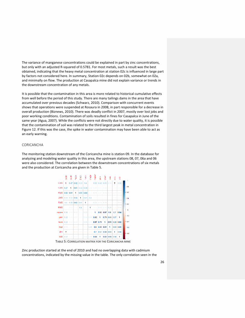
CORICANCHA The monitoring station downstream of the Coricancha mine is station 09. In the database for analyzing and modeling water quality in this area, the upstream stations 08, 07, 06a and 06 were also considered. The correlation between the downstream concentrations of six metals and the production at Coricancha are given in Table 5.

TABLE 5: CORRELATION MATRIX FOR THE CORICANCHA MINE

Zinc production started at the end of 2010 and had no overlapping data with cadmium concentrations, indicated by the missing value in the table. The only correlation seen in the

27

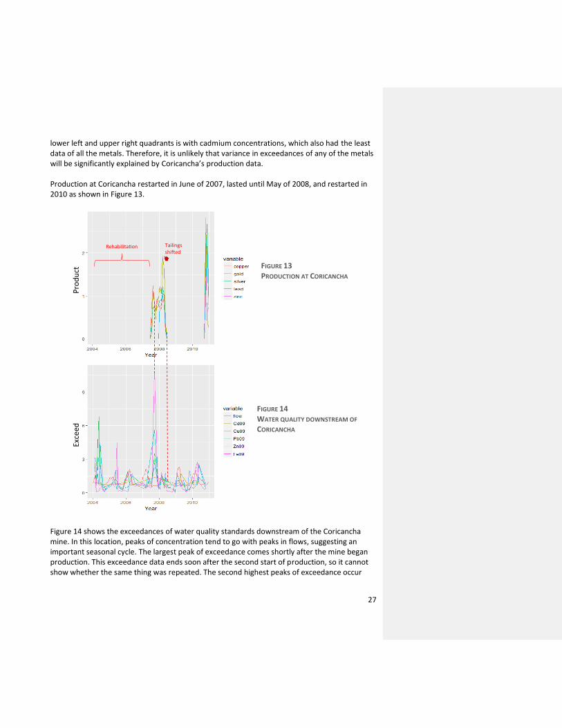
lower left and upper right quadrants is with cadmium concentrations, which also had the least data of all the metals. Therefore, it is unlikely that variance in exceedances of any of the metals will be significantly explained by Coricancha’s production data. Production at Coricancha restarted in June of 2007, lasted until May of 2008, and restarted in 2010 as shown in Figure 13.

FIGURE 13 PRODUCTION AT CORICANCHA

FIGURE 14 WATER QUALITY DOWNSTREAM OF

CORICANCHA

Figure 14 shows the exceedances of water quality standards downstream of the Coricancha mine. In this location, peaks of concentration tend to go with peaks in flows, suggesting an important seasonal cycle. The largest peak of exceedance comes shortly after the mine began production. This exceedance data ends soon after the second start of production, so it cannot show whether the same thing was repeated. The second highest peaks of exceedance occur

Exce

edan

ce

Pro

du

ctio

n

Rehabilitation Tailings shifted

28

when the mine is not operating, indicating that other factors are responsible for the heavy metal loading in Rimac in those instances. Modeling downstream water quality showed that zinc at station 09 was best explained by zinc at station 08 and 07, and less importantly by lead production. Even using all three variables, the residual error was 47% (𝑅2=0.2822, p-value=0.0027). Comparison with key events explains the extreme changes in production and possibly heavy metal loadings not captured in the model parameters. The mine was under rehabilitation until 2007, so it is possible that infrastructure work released metals into the environment. Production stopped again in 2008 when the mine detected that a nearby agricultural irrigation system was causing ground displacement at a tailings dam, according to the company that owned the mine (Oracle, 2017). Other causes suggested include flooding due to intense rains or seismic activity (Kirwin, 2008). It is notable that shifting near tailings, which has the potential to cause a significant release of heavy metals, did not cause a peak in exceedances. This indicates that the potential problem was addressed in time such that it did not noticeably affect heavy metal concentrations. The closure was followed by a period of relatively low concentrations, with no measurement exceeding the water quality standard by more than 100%.

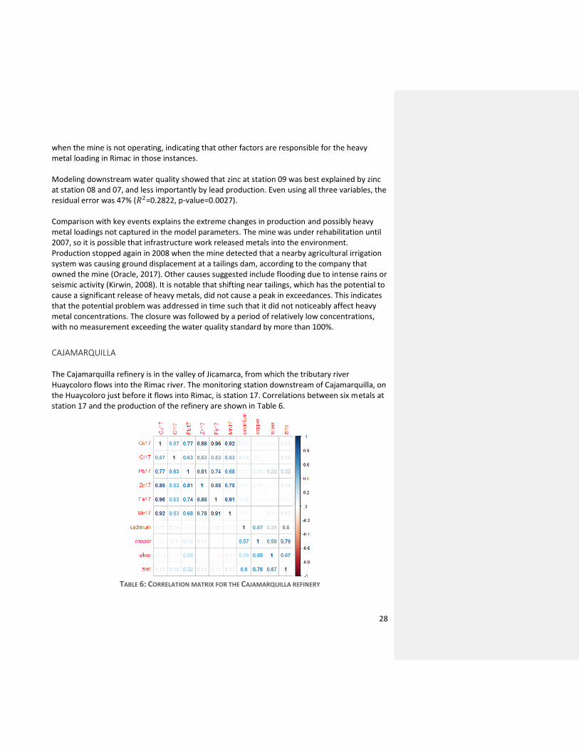
CAJAMARQUILLA The Cajamarquilla refinery is in the valley of Jicamarca, from which the tributary river Huaycoloro flows into the Rimac river. The monitoring station downstream of Cajamarquilla, on the Huaycoloro just before it flows into Rimac, is station 17. Correlations between six metals at station 17 and the production of the refinery are shown in Table 6.

TABLE 6: CORRELATION MATRIX FOR THE CAJAMARQUILLA REFINERY

29

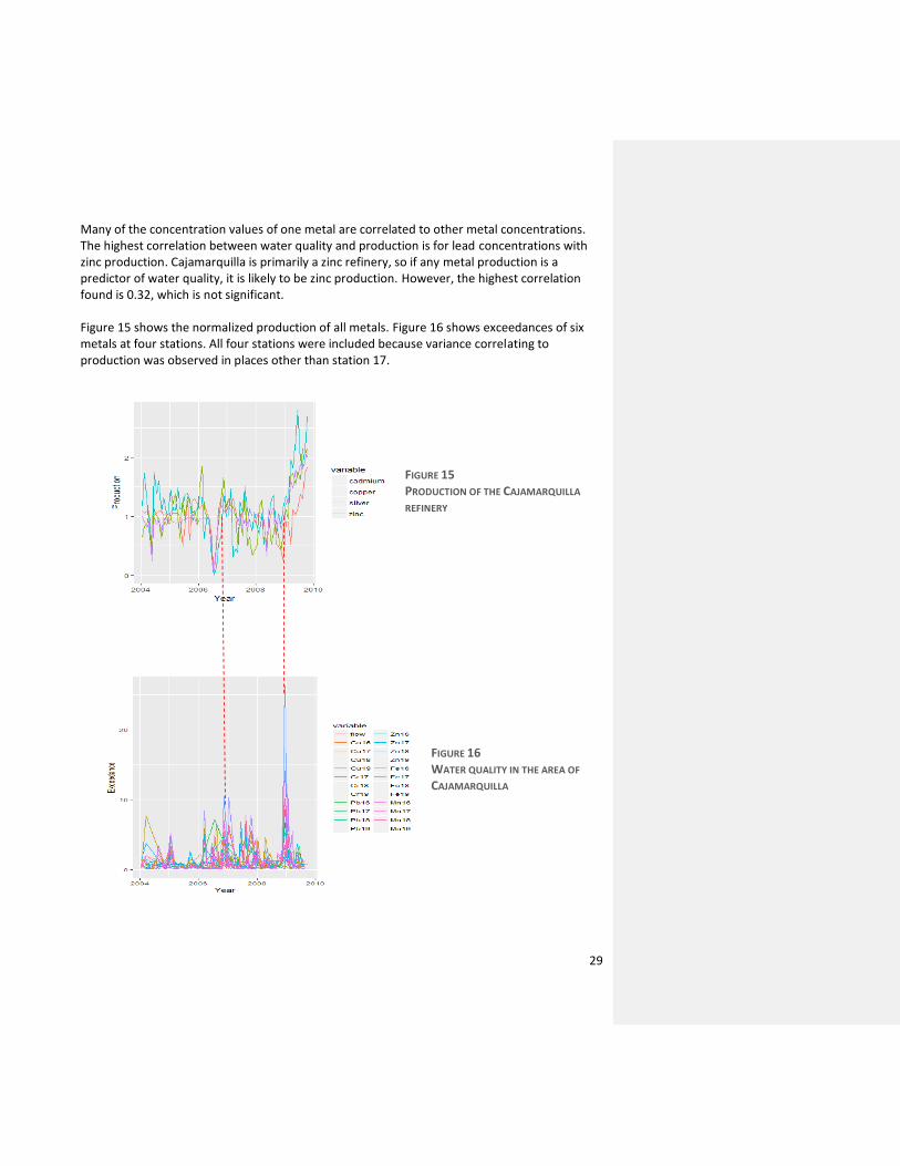
Many of the concentration values of one metal are correlated to other metal concentrations. The highest correlation between water quality and production is for lead concentrations with zinc production. Cajamarquilla is primarily a zinc refinery, so if any metal production is a predictor of water quality, it is likely to be zinc production. However, the highest correlation found is 0.32, which is not significant. Figure 15 shows the normalized production of all metals. Figure 16 shows exceedances of six metals at four stations. All four stations were included because variance correlating to production was observed in places other than station 17.

FIGURE 15 PRODUCTION OF THE CAJAMARQUILLA

REFINERY

FIGURE 16 WATER QUALITY IN THE AREA OF

CAJAMARQUILLA

30

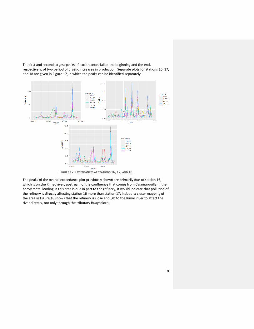
The first and second largest peaks of exceedances fall at the beginning and the end, respectively, of two period of drastic increases in production. Separate plots for stations 16, 17, and 18 are given in Figure 17, in which the peaks can be identified separately.

FIGURE 17: EXCEEDANCES AT STATIONS 16, 17, AND 18.

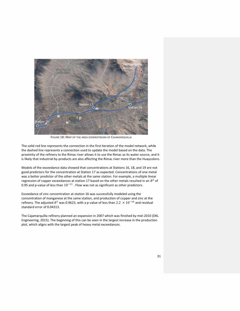
The peaks of the overall exceedance plot previously shown are primarily due to station 16, which is on the Rimac river, upstream of the confluence that comes from Cajamarquilla. If the heavy metal loading in this area is due in part to the refinery, it would indicate that pollution of the refinery is directly affecting station 16 more than station 17. Indeed, a closer mapping of the area in Figure 18 shows that the refinery is close enough to the Rimac river to affect the river directly, not only through the tributary Huaycoloro.

31

FIGURE 18: MAP OF THE AREA DOWNSTREAM OF CAJAMARQUILLA

The solid red line represents the connection in the first iteration of the model network, while the dashed line represents a connection used to update the model based on the data. The proximity of the refinery to the Rimac river allows it to use the Rimac as its water source, and it is likely that industrial by-products are also affecting the Rimac river more than the Huaycoloro. Models of the exceedance data showed that concentrations at Stations 16, 18, and 19 are not good predictors for the concentration at Station 17 as expected. Concentrations of one metal was a better predictor of the other metals at the same station. For example, a multiple linear regression of copper exceedances at station 17 based on the other metals resulted in an 𝑅2 of 0.95 and p-value of less than 10−11 . Flow was not as significant as other predictors. Exceedance of zinc concentration at station 16 was successfully modeled using the concentration of manganese at the same station, and production of copper and zinc at the refinery. The adjusted 𝑅2 was 0.9623, with a p-value of less than 2.2 × 10−16 and residual standard error of 0.04313. The Cajamarquilla refinery planned an expansion in 2007 which was finished by mid-2010 (DKL Engineering, 2015). The beginning of this can be seen in the largest increase in the production plot, which aligns with the largest peak of heavy metal exceedances.

32

CONCLUSIONS There was very little temporal trend in contamination in the Rimac basin, over the seven years considered. This is likely due to the long history of mining in the region, which makes a seven-year period insufficient to detect long-term trends. It is a possible indicator of temporal cumulative effects already well underway. If the ecosystems are already impacted by past mining, then it is difficult to distinguish a measurable impact of current mining production on contamination. It’s also possible that there are other mine-related parameters that are more predictive than monthly production, such as amount of waste deposited or remediation expenditures. The spatial trend was distinct, with increased metal concentration in the upper and lower parts of the basin. It was not explained by production, nor trends over time nor completely by the localization of the mining activity. Using river flow at one location over time did not explain the contamination, but it is possible that the spatial dimension of flow can help predict contamination levels. Perhaps concentrations, which are used for water quality standards, are not the best metric for understanding accumulation of heavy metals from mining. Total mass may be more influenced by mine production. Even so, the locations of water quantity addition and extraction did not completely correspond to the spatial changes in contamination. It is likely that cumulative effects are at play in the spatial dimension as well. For all three smaller areas of the basin considered, modeling zinc downstream of a mine was most successful. This compares well with previous studies: “zinc found in the water samples is likely to come from the polymetallic mines situated in the region” (Méndez, 2005), whereas lead, for example, may be due in part to active mines but is also likely influenced by a large abandoned mine (MEM, 1997). The predictor variables for a given metal were different for each area. In some instances, the best covariates were different metals at the same station. In others, it was exceedances of the same metal, one or two stations upstream. Exceedance data more than two stations upstream was not significant in any of the places studied. At the Coricancha refinery, the production of two metals at the nearby mine helped explain some of the variance. Flow was not a key variable in the main three regression models, but could become important if seasonality is more directly incorporated into a model. In some places and for certain metals, no suitable model was found using the inputs of this study. This is also an important result, indicating that additional variables such as natural leaching, informal mining, and legacy sites may contribute significantly to the heavy metal loading. Exogenous variables such as conflict and changes in mine operation also seem to be important yet complicated factors. While conflict may affect mine production and therefore can indirectly affect water quality, poor water quality may also affect or instigate conflict. The 2008 regulation change was not obvious in this data and would be more important in a study that uses data beyond 2010.

33

Model improvements would be possible with more consistency in sampling. Institutional changes caused the sampling frequency to decrease after 2011. It is ironic that we hoped to observe improvements in water quality after legal improvements related to water quality. However, the most distinct observation has been that an institutional restructuring led to a decrease in data. It now is less useful and less frequent that data used in this study, which already was not sufficient for complete trend attribution. The way data is collected creates a challenge for modeling, as does the presence of legacy sites with little information. Consistency in reporting and use of databases rather than paper reports would enable comparison and inclusion of additional data sources. The geographic data is a limiting factor to the scalability of this study, as we had to confirm the mine locations and alternative mine names individually. A more complete mining database with geographic information is necessary to do similar work on a larger scale. First-hand knowledge of an area is essential for constructing the initial network and identifying what are possible influences on water quality. Even then, we recommend a methodology that can reconstruct the network or re-assign importance of each connection stochastically based on the data. At Coricancha, the results of modeling water quality exceedances suggested a network connection that was not previously incorporated. Automatic determination of which factors are most important for each monitoring station, based on the data, would be an important development in moving from modeling sub-regions of the basin to a basin-level model. This could be well supported by a machine learning algorithm. Using such a model to iterate the possible inputs and determine which are significant would allow a more exhaustive approach and robust model evaluation than was done in this study. Though having surface flow models could be helpful, that alone would not have sufficiently predicted the direction of contamination in the Rimac basin. A combination of physical and stochastic model is recommended. Perhaps most importantly, all metals studied exceeded the water quality standards at least once each year. If mines usually meet the Maximum Permissible Limit in their effluent, then clearly these MPLs are not accurately considering cumulative effects. Modelling such as is done here can help identify which mines are most contributing to exceedance of a given metal at a given location. This would allow permitting to be done such that it considers the local conditions and cumulative effects. The results of the model would be helpful information for a mine in meeting their MPLs, because it can show if a given amount of pollution is proportional to the production, rather than it being a constant source or a binary factor related to whether the mine is operational or non-operational. A model also enables discretion in not being unnecessarily stringent on discharge limits. If a mine's production isn't directly linked to exceedance of ECAs, then other causal relationships need to be explored before taking action. In the case of the Rimac basin, it seems that mining is having a significant impact on the water quality. This may eventually lead to external liability for the mines due to long-term impacts on the largest metropolitan area. The likelihood of cumulative effects, both in space and time, indicate that remediation is needed. Also important is future study using more complete data, to attribute the contamination to the probable sources.

34

APPENDICES

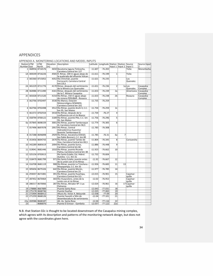
APPENDIX A. MONITORING LOCATIONS AND MODEL INPUTS Station

Number UTM East

UTM North

Elevation (m)

Description Latitude Longitude Station Input 1

Station Input 2

Source Input 1

Source Input 2

1 368956 8716576 4650 Bocatoma laguna Ticticocha, Carretera Central km 127

-11.607 -76.202 Ticlio Morochocha

1A 369249 8716226 4565 R. Rímac, 100 m aguas abajo de la quebrada del efluente Volcan

-11.611 -76.199 1 Ticlio

2 365360 8715052 4352 Río Chinchán, puente Ferrocarril, Carretera Central km119,5

-11.621 -76.235 Los Quenales

2A 365229 8711776 4170 Rímac, después del vertimiento de la Minera Los Quenuales

-11.651 -76.236 2 1a Los Quenales

Casapalca Complex

2B 364986 8711490 4161 Rímac, después del vertimiento de la C. Minera Casapalca

-11.653 -76.239 2a Americana Casapalca Complex

2C 365028 8711520 4154 Río Rímac, 150 m aguas abajo de minera PERUBAR - Rosaura

-11.653 -76.238 2b Rosaura Casapalca Complex

3 362766 8702497 3530 Río Blanco, Estación Meteorológica SENAMHI, Carretera Central km 101

-11.735 -76.259

4 362766 8702498 3512 Río Rímac, puente Anchi II, C.C. km 95, San Mateo

-11.734 -76.259 2c

5 361572 8702554 3418 Río Rímac, después de la confluencia con el río Blanco

-11.734 -76.27 4

6 358794 8700122 3189 Río Rímac, puente Pite, C.C. km 95, San Mateo

-11.756 -76.296 5

6a 357845 8698159 3001 Río Rímac, puente Tamboraque III, Carretera Central km 90,5

-11.774 -76.305 6

7 357496 8697078 2957 Río Rímac, Central Hidroeléctrica Huanchor (puente Tamboraque II)

-11.783 -76.308

8 357288 8696898 2929 Río Rímac, bocatoma EDEGEL (ex Pablo Bonner), C.C. km 89

-11.785 -76.31 6a 7

9 353456 8694743 2670 Río Rímac, puente Tambo de Viso, Carretera Central km 83,5

-11.804 -76.345 8 Coricancha

10 342289 8685619 2004 Río Rímac, puente Surco, Carretera Central km 66

-11.886 -76.448 9

11 319041 8681446 1010 Río Rímac, puente Ricardo Palma, Carretera Central km 38

-11.923 -76.662 10

12 325156 8702613 Río Santa Eulalia, Est. Hidrol. Autisha - C.C. Km 31

-11.732 -76.604

13 318479 8681799 971 Río Santa Eulalia, puente antes de la unión con el río Rímac

-11.92 -76.667 12

14 316708 8681119 908 Río Rímac, puente La Trinchera - Moyopampa, C.C. km 35

-11.926 -76.683 11 13

15 305656 8675326 642 Río Rímac, puente Morón, Carretera Central km 23

-11.977 -76.785 14

16 293037 8671081 391 Río Rímac, puente Huachipa, Carretera Central Km 9,5

-12.015 -76.901 15 Cajamar-quilla

17 287452 8670464 303 Río Huaycoloro, antes de la unión con el río Rímac

-12.02 -76.952 Cajamar-quilla

18 286517 8670066 287 Río Rímac, Mirador Nº 1 Las Palmeras

-12.024 -76.961 16 17 Cajamar-quilla

19 278886 8667889 Puente Santa Rosa -12.043 -77.031 18 20 275178 8668746 Puente Dueñas -12.035 -77.065 19 21 272494 8668412 Altura Av. Victor A. Belaunde -12.038 -77.09 20 22 271259 8668126 Puente Faucett a 50m de

desembocadura de vertimiento -12.04 -77.101 21

22a 269586 8668187 Alt. Av. Santa Rosa -12.04 -77.116 22 23 8686876 Puente El Emisor - Gambeta -12.037 -77.122 22a

N.B. that Station 02c is thought to be located downstream of the Casapalca mining complex, which agrees with its description and patterns of the monitoring network design, but does not agree with the coordinates given here.

35

APPENDIX B: EXCEEDANCE TIME SERIES AND MANN KENDALL TESTS AT UPSTREAM STATIONS

36

APPENDIX C: EXCEEDANCE RATIO FOR EACH METAL, EXCLUDING DATA AT THE DETECTION LIMIT.

37

APPENDIX D: PRODUCTION BY METAL, FOR ALL MINES IN RIMAC.

38

REFERENCES Agua, La revista del recurso hídrico de Chile. Multan a minera Casapalca por contaminación. Published 24-Aug-2007, retrieved at www.revistagua.cl/2007/08/24/peru-multan-a-minera-casapalca-por-contaminacion/

Autoridad Nacional del Agua. Evaluación de los Recursos Hídricos en la Cuenca del Río Rímac. Lima (2010).

Autoridad Nacional del Agua. Sistema de adquisición de datos hídricos online. Retrieved from snirh.ana.gob.pe/sadho (2014).

Badaoui, H.E. et al. Application of the artificial neural networks of MLP type for the prediction of the levels of heavy metals in Moroccan aquatic sediments. IJCER 3(6) (2011).

Bebbington, A. and Williams, M. Water and mining conflicts in Peru. Mountain Research and Development 28(3/4):190-195. www.bioone.org/doi/pdf/10.1659/mrd.1039 (2008).

Biznews. Perubar vende ‘Rosaura’ a Los Quenuales. Published 23-Apr-2010. Retrieved at biznews.pe/noticias-empresariales-nacionales/perubar-vende-rosaura-los-quenuales

Budds, J. The expansion of mining and changing waterscapes in the southern Peruvian Andes. In Norman, E. (Ed.) Negotiating Water Governance: Why the Politics of Scale Matter. 215-230 (2015).

Buszewski, B. A new model of heavy metal transport in the soil using nonlinear artificial neural networks. Environ Eng Sci 23(4) 589-595 (2006).

Calla, H. J. Calidad del agua en la cuenca del Río Rímac - Sector de San Mateo, afectado por las actividades mineras. Thesis, Universidad Nacional Mayor de San Marcos (2010).

Church, S.E., von Guerard, Paul, and Finger, S.E. Impacts of Historical Mining on Aquatic Ecosystems—An Ecological Risk Assessment. Integrated investigations of environmental effects of historical mining in the Animas River watershed, San Juan County, Colorado: U.S. Geological Survey Professional Paper 1651, 1(D) (2007).

Chibuike, G. U. and Obiora, S. C. Heavy metal polluted soils: Effect on plants and bioremediation methods. Applied and Environmental Soil Science, 2014 (2014).

Council on Environmental Quality. Considering Cumulative Effects Under the National Environmental Policy Act. Retrieved at https://energy.gov/sites/prod/files/nepapub/nepa_documents/RedDont/G-CEQ-ConsidCumulEffects.pdf (1997).

Crivineanu, M. F., Perju, D., Dumitrel, G., Perju, D.S. Mathematical Models Describing the emission and Distribution of Heavy Metals in Surface Waters. Rev. Chim. 63:4 (2012).

Commented [LB3]: Make Word References

39

Dirección General de Salud Ambiental. Vigilancia y monitoreo de los recursos hídricos. Retrieved from http://digesa.sld.pe/depa/vigilancia_recursos_hidricos.asp (2010).

DKL Engineering. Acid Plant Database. Retrieved at www.sulphuric-acid.com/sulphuric-acid-on-the-web/acid%20plants/Cajamarquilla%20Refinery.htm (2015).

El Peruano Normas Legales. Decreto Supremo #015-2015-MINEM. Published 19-Dec-2015.

Environmental Law Alliance Worldwide. Guía para evaluar EIAs de proyectos mineros. Retrieved at www.elaw.org/es/content/guí-para-evaluar-eias-de-proyectos-mineros (2010).

Ernst&Young. Peru’s mining & metals investment guide. Lima: Ernst & Young. (2015).

Gillespy, M. Drying and Drowning Assets. Presentation at the Second Annual Global Workshop on Mining-related Water and Environmental Risks and their Financial Implications. New York, NY. (2016).

Hanikenne, M., Merchant, S., and Hamel, P. Transition metal nutrition: A balance between deficiency and toxicity. In Stern, D. (Ed.) Organellar and Metabolic Processes. Netherlands: Elsevier Science Bv. 333-339 (2009).

Hubner, R., Astin, K.B., and Herbert, R. ‘Heavy metal’—time to move on from semantics to pragmatics? J. Environ. Monit., 12(8) (2010).

Interntional Council on Mining and Metals. Water management in mining: a selection of case studies. Retrieved at http://hub.icmm.com/document/3660 (2012).

Interntional Council on Mining and Metals. A practical guide to catchment-based water management for the mining and metals industry. Retrieved at www.icmm.com/website/publications/pdfs/8329.pdf (2015).

Juarez, H. Contaminación del Río Rímac por metales pesados y efecto en la agricultura en el Cono Este de Lima Metropolitana. Retrieved at www.aguasanperu.org/Docs/CalidadDeAguaEnElRioRimac.pdf (2012).

Kaveney, T., Kerswell, A. and Buick, A. Cumulative Environmental Impact Assessment Industry Guide. Minerals Council of Australia. Retrieved at www.minerals.org.au/leading_practice/cumulative_impact_assessment (2015).

Kirwin, S. Gold Hawk cierra temporalmente mina Coricancha. The Northern Miner, Published 2-Jun-2008, retrieved at www.conflictosmineros.net/contenidos/19-peru/4299-4299

K-Water, Yooshin Engineering, and Pyunghwa Engineering. Plan maestro del proyecto restauración del río Rímac. Consulting report for the Peruvian National Water Authority. (2015).

Llontop, H. J. Calidad del agua en la cuenca del Río Rímac - Sector de San Mateo, afectado por las actividades mineras. Thesis, Universidad Nacional Mayor de San Marcos (2010).

40

Méndez, W. Contamination of Rimac river basin Peru, due to mining tailings. Thesis, KTH Architecture and the built Environment (2005).

Ministerio de Energía y Minas. Evaluación Ambiental Territorial de la Cuenca del Río Rímac. Dirección General de Asuntos Ambientales. Lima, p48 (1997).

Minesterio de Energia y Minas. Ventanilla virtual. Retrieved from www.minem.gob.pe/_estadisticaSector.php?idSector=1&idCategoria=10&pagina=1 (2016).

Oracle Mining Corp. History. Retrieved at www.oracleminingcorp.com/history/ (2016).

Ramos, W. et. al. Noninfectious dermatological diseases associated with chronic exposure to mine tailings in a Peruvian district. Br J Dermatol. 159(1):169-74 (2008).

Rivera, H., Chira, J., Zambrano, K., and Peterson, P. Dispersión secundaria de los metales pesados en sedimentos de los ríos Chillón, Rímac y Lurín Departamento de Lima. Revista del Instituto de Investigaciones FIGMMG 10(20) 19-25 (2007).

Rooki, R. et al. Prediction of heavy metals in acid mine drainage using artificial neural network from the Shur River of the Sarcheshmeh porphyry copper mine, Southeast Iran. Environ Earth Sci. 64(5) 1303–1316 (2011).

Slack, K. The growing battle between mining and agriculture. Oxfam Politics of Poverty

politicsofpoverty.oxfamamerica.org/2013/04/the-growing-battle-between-mining-and-agriculture/ (2013).

SNL. Metals and mining database. Retrieved from www.snl.com/Sectors/MetalsMining/ (2016).

Solomon, R. et al. Cumulative Effects Analyses for NEPA Documents. Shipley Newsletter XX (2016).

Schwarz, G.E., Hoos, A.B., Alexander, R.B. and Smith, R.A. The SPARROW surface water-quality model: Theory, application and user documentation. U.S. Geological Survey Techniques and Methods 6–B3, 248 (2006).

Zoi Environment network. The journey of Rimac. Retrieved at www.zorimac.org (2014).