modeling and control of solid oxide fuel cell –...
TRANSCRIPT

MODELING AND CONTROL OF SOLID OXIDE FUEL CELL – GAS TURBINE POWER PLANT SYSTEMS
by
Adam Hahn
BS, University of Pittsburgh, 2000
Submitted to the Graduate Faculty of
School of Engineering in partial fulfillment
of the requirements for the degree of
Master of Science in Mechanical Engineering
University of Pittsburgh
2004

ii
UNIVERSITY OF PITTSBURGH
SCHOOL OF ENGINEERING
This thesis was presented
by
Adam Hahn
It was defended on
April 8, 2004
and approved by
Sung Kwon Cho, Assistant Professor, Department of Mechanical Engineering
William Clark, Associate Professor, Department of Mechanical Engineering
Thesis Advisor: Jeffrey Vipperman, Assistant Professor, Department of Mechanical Engineering

iii
MODELING AND CONTROL OF SOLID OXIDE FUEL CELL – GAS TURBINE POWER PLANT SYSTEMS
Adam Hahn, MSME
University of Pittsburgh, 2004
There is extensive research taking place involving fuel cell – gas turbine combined power plant
systems. These systems use a high temperature fuel cell and a gas turbine to achieve higher
overall performance and efficiency than a single mode power plant. Due to the high temperature
of the exhaust gasses of the fuel cell, heat can be recuperated and used to drive a gas turbine.
The turbine creates additional power and is a means of utilizing the exhaust energy of the fuel
cell. Despite the research being done on integrating these systems, little work has been done to
characterize the dynamics of the integrated systems. Due to the high response of the fuel cell
and the relatively sluggish response of the turbine, control of the system needs to be understood.
This thesis develops dynamic models of the individual components that comprise a fuel cell –
gas turbine hybrid system (axial flow compressor, combustor, turbine, fuel cell, and heat
exchanger). These models are incorporated to produce a complete dynamic hybrid model. The
models are analyzed with respect to dynamics and basic control techniques are used to control
various parameters. It is shown that the system can be controlled using hydrogen input flow rate
control for the fuel cell and controlled turbine inlet temperature for the gas turbine.

iv
TABLE OF CONTENTS
1.0 INTRODUCTION .............................................................................................................. 1
1.1 FUEL CELL POWER PLANTS .................................................................................... 1
1.2 GAS TURBINES............................................................................................................ 2
1.3 COMBINED FUEL CELL GAS TURBINE POWER PLANTS................................... 3
1.4 CURRENT STUDY AND ORGANIZATION .............................................................. 5
2.0 GAS TURBINE MODELS................................................................................................. 7
2.1 AXIAL FLOW COMPRESSOR .................................................................................... 7
2.1.1 Main Operating Theory........................................................................................... 8
2.1.2 Compressor Characteristics .................................................................................. 11
2.1.3 Moore Greitzer Model .......................................................................................... 12
2.1.4 Exit Ducts and Guide Vanes ................................................................................. 17
2.1.5 Compressor Characteristic .................................................................................... 20
2.1.6 Galerkin Procedure ............................................................................................... 21
2.1.7 Spool Dynamics .................................................................................................... 23
2.1.8 Compressor Model Simulation ............................................................................. 27
2.2 COMBUSTOR.............................................................................................................. 40
2.2.1 Combustor Model ................................................................................................. 42
2.2.2 Combustor Model Simulation............................................................................... 48

v
2.3 TURBINE ..................................................................................................................... 55
2.3.1 Turbine Theory ..................................................................................................... 55
2.3.2 Turbine Function................................................................................................... 56
2.3.3 Turbine Function Simulation ................................................................................ 58
3.0 HEAT EXCHANGER AND FUEL CELL MODELS ..................................................... 60
3.1 HEAT EXCHANGER .................................................................................................. 60
3.1.1 Heat Exchanger Theory ........................................................................................ 60
3.1.2 Heat Exchanger model.......................................................................................... 62
3.1.3 Heat Exchanger Model Simulation....................................................................... 64
3.2 FUEL CELL.................................................................................................................. 70
3.2.1 Fuel Cell Operating Theory .................................................................................. 70
3.2.2 Fuel Cell Model .................................................................................................... 72
3.2.3 Fuel Cell Model Simulation.................................................................................. 78
4.0 MODEL INTEGRATION ................................................................................................ 83
4.1 GAS TURBINE INTEGRATION ................................................................................ 83
4.1.1 Gas Turbine Model Integration............................................................................. 83
4.1.2 Gas Turbine Model Simulation............................................................................. 85
4.2 FUEL CELL – GAS TURBINE ................................................................................... 88
4.2.1 FCGT – Integration Configuration One................................................................ 88
4.2.2 FCGT – Integration Configuration One Simulation ............................................. 91
4.2.3 FCGT – Integration Configuration Two............................................................... 93
4.2.4 FCGT – Integration Configuration Two Simulation ............................................ 94
5.0 PRELIMINARY CONTROLS ......................................................................................... 99

vi
5.1 RESPONSE TO A STEP INPUT ................................................................................. 99
5.2 TURBINE ROTOR SPEED CONTROL.................................................................... 104
6.0 CONCLUSIONS AND FUTURE WORK ..................................................................... 112
BIBLIOGRAPHY....................................................................................................................... 114

vii
LIST OF TABLES Table 1: Compressor Simulation Parameters............................................................................... 27
Table 2: Combustor Simulation Model Parameters..................................................................... 49
Table 3: Heat Exchanger Simulation Parameters ........................................................................ 64
Table 4: Fuel Cell Simulation Parameters ................................................................................... 78
Table 5: Step Input Response Simulation Parameters ............................................................... 100
Table 6: Air Inject PID Control Settings ................................................................................... 105

viii
LIST OF FIGURES
Figure 1: Axial Compressor Rotor and Stator Diagrams............................................................... 9
Figure 2: Airflow Around a Stalled Airfoil ................................................................................. 10
Figure 3: Typical Axial Flow Compressor Characteristic ........................................................... 12
Figure 4: Moore – Greitzer Compressor Model .......................................................................... 13
Figure 5: Dimensionless Flow Rate (Φ), Unstable Condition...................................................... 29
Figure 6: Dimensionless Pressure Ratio (Ψ), Unstable Condition............................................... 29
Figure 7: Stall Coefficient (J), Unstable Condition ...................................................................... 30
Figure 8: Dimensionless Compressor Speed (B), Unstable Condition ........................................ 30
Figure 9: Dimensionless Flow Rate (Φ), Stable Condition .......................................................... 32
Figure 10: Dimensionless Pressure Ratio (Ψ), Stable Condition................................................. 32
Figure 11: Stall Coefficient (J), Stable Condition ....................................................................... 33
Figure 12: Dimensionless Compressor Speed (B), Stable Condition .......................................... 33
Figure 13: Simulink Model of Axial Flow Compressor .............................................................. 35
Figure 14: Simulink Compressor Model Results, Flow Rate (Φ), Unstable Condition .............. 36
Figure 15: Simulink Compressor Model Results, Pressure Ratio (Ψ), Unstable Condition........ 36
Figure 16: Simulink Compressor Model Results, Compressor Speed (B), Unstable Condition . 37
Figure 17: Simulink Compressor Model Results, Stall Coefficient (J), Unstable Condition...... 37
Figure 18: Simulink Compressor Model Results, Flow Rate (Φ), Stable Condition .................. 38

ix
Figure 19: Simulink Compressor Model Results, Pressure Ratio (Ψ), Stable Condition ............ 38
Figure 20: Simulink Compressor Model Results, Compressor Speed (B), Stable Condition...... 39
Figure 21: Simulink Compressor Model Results, Stall Coefficient (J), Stable Condition .......... 39
Figure 22: Typical Gas Turbine Cycle......................................................................................... 41
Figure 23: Temperature – Entropy Diagram of Typical Gas Turbine Cycle............................... 41
Figure 24: Conservation of Species of Combustor ...................................................................... 43
Figure 25: Linear Curve Fit of Internal Energy of Products........................................................ 47
Figure 26: Linear Curve Fit of Enthalpy of Products and Air ..................................................... 47
Figure 27: Outlet Fluid Temperature ........................................................................................... 49
Figure 28: Fuel Mass Fraction Inside Combustor........................................................................ 50
Figure 29: Oxidizer Mass Fraction Inside Combustor................................................................. 50
Figure 30: Combustor Model in Simulink Using S-Function...................................................... 52
Figure 31: Output Temperature of Simulink Combustor Model ................................................. 52
Figure 32: Output Flow Rate of Simulink Combustor Model ..................................................... 53
Figure 33: Mass Flow Rate of Combustor Model with Varying Input Air Flow Rate................ 54
Figure 34: Output Temperature of Simulink Combustor Model with Varying Oxidizer Input Flow Rate .............................................................................................................................. 54
Figure 35: Example Turbine Stage .............................................................................................. 56
Figure 36: Simulink Turbine Function ........................................................................................ 58
Figure 37: Turbine Torque Generated from Uncoupled Turbine Simulation.............................. 59
Figure 38: Net Power Out from Uncoupled Turbine Simulation ................................................ 59
Figure 39: Temperature Graph of Counter Flow Heat Exchanger .............................................. 61
Figure 40: Heat Exchanger Simulink S-Function........................................................................ 65
Figure 41: Mass Flow Rate of Cold Stream – Heat Exchanger Model ....................................... 66

x
Figure 42: Mass Flow Rate of Hot Stream – Heat Exchanger Model ......................................... 66
Figure 43: Outlet Temperature of Cold Stream – Heat Exchanger Model .................................. 67
Figure 44: Outlet Temperature of Hot Stream – Heat Exchanger Model.................................... 67
Figure 45: Mass Flow Rate of Cold Stream – Heat Exchanger Model with Higher Cold Mass Flow Rate .............................................................................................................................. 68
Figure 46: Mass Flow Rate of Hot Stream – Heat Exchanger Model with Higher Cold Mass
Flow Rate .............................................................................................................................. 69 Figure 47: Temperature Out of Cold Stream – Heat Exchanger Model with Higher Cold Mass
Flow Rate .............................................................................................................................. 69 Figure 48: Temperature Out of Hot Stream – Heat Exchanger Model with Higher Cold Mass
Flow Rate .............................................................................................................................. 70 Figure 49: Solid Oxide Fuel Cell ................................................................................................. 71
Figure 50: Simulink Fuel Cell Model .......................................................................................... 79
Figure 51: Fuel Cell Simulation Parameters................................................................................ 80
Figure 52: Fuel Cell Voltage........................................................................................................ 80
Figure 53: Fuel Cell Power .......................................................................................................... 81
Figure 54: Fuel Cell Voltage Response Due to Linear Current Ramp ........................................ 82
Figure 55: Gas Turbine Simulink Model ..................................................................................... 84
Figure 56: Gas Turbine Output Power......................................................................................... 86
Figure 57: Gas Turbine Rotor Angular Velocity ......................................................................... 87
Figure 58: Turbine Inlet Temperature.......................................................................................... 87
Figure 59: Fuel Cell Gas Turbine Integration using Heat Exchanger ......................................... 89
Figure 60: Fuel Cell Gas Turbine Hybrid Power Plant Simulink Model .................................... 90
Figure 61: FCFT Power Plant – Fuel Cell Power ........................................................................ 91
Figure 62: FCFT Power Plant – Gas Turbine Power................................................................... 92

xi
Figure 63: FCFT Power Plant – Gas Turbine Rotor Angular Velocity ....................................... 92
Figure 64: FCFT Power Plant – Total Plant Power ..................................................................... 93
Figure 65: Fuel Cell Gas Turbine Hybrid Power Plant Configuration Two................................ 94
Figure 66: Fuel Cell Gas Turbine Hybrid Power Plant Simulink Model Configuration Two..... 96
Figure 67: FCGT Configuration Two – Fuel Cell Power ............................................................ 97
Figure 68: FCGT Configuration Two – Gas Turbine Power....................................................... 97
Figure 69: FCGT Configuration Two – Gas Turbine Rotor Angular Velocity ........................... 98
Figure 70: FCGT Configuration Two – Total Plant Power ......................................................... 98
Figure 71: Fuel Cell Power during a Hydrogen Mass Flow Step Change................................. 101
Figure 72: Gas Turbine Power during a Hydrogen Mass Flow Step Change............................ 101
Figure 73: Rotor Angular Velocity during a Hydrogen Mass Flow Step Change..................... 102
Figure 74: Total Plant Power during a Hydrogen Mass Flow Step Change.............................. 102
Figure 75: Total Plant Power during a Throttle Coefficient Step Input .................................... 103
Figure 76: Pressure Output of Compressor during a Throttle Coefficient Step Input ............... 104
Figure 77: Angular Velocity with Control – PID gain settings 1 – Unstable ............................ 106
Figure 78: Angular Velocity with Control – PID gain settings 2 – Semi-stable ....................... 107
Figure 79: Angular Velocity with Control – PID gain settings 3 – Stable with Oscillations .... 108
Figure 80: Angular Velocity with Control – PID gain settings 4 – Stable ................................ 109
Figure 81: Angular Velocity with Control – Stepped Setpoint – Stable.................................... 110
Figure 82: Fuel Cell Power Reaction to Step in Rotor Angular Velocity .................................. 111

xii
To Susan

1
1.0 INTRODUCTION
1.1 FUEL CELL POWER PLANTS
Fuel cells have been receiving a lot of attention lately due to their potential as becoming a new
energy source with a large range of applications. The benefits of fuel cell energy are primarily
the high efficiency with which they can run and their environmentally friendly by-products. Fuel
cells use a chemical reaction to convert hydrogen and oxygen into water, releasing electrons
(energy) in the process. Essentially, the hydrogen fuel is being “burnt” in a simple reaction to
produce water. Instead of releasing energy, however, the reaction releases an electric current. A
typical fuel cell consists of two electrodes (anode and cathode) where the reactions take place.
The electrodes are also the mediums that the current flows between. Sandwiched between the
electrodes is an electrolyte material which the ions flow through to keep the reactions
continuous. There are several types of fuel cells being researched at present. These include
alkaline, proton exchange membrane, phosphoric acid, molten carbonate, and solid oxide. They
differ in electrode and electrolyte materials, chemical reactions, catalysts, and operating
temperatures and pressures [8].

2
Fuel cells can be incorporated with other components to create high efficiency industrial power
plants. These power plants usually consist of a pump or blower to circulate the working fluids
through the fuel cell, a reformer to convert the fuel into hydrogen, pressure regulators, and power
conditioners. Most fuel cells do not use straight hydrogen as fuel. Therefore they must
incorporate a reformer to convert the fuel being used into hydrogen. Fuels that can be reformed
are methane, ammonia, methanol, ethanol, or gasoline. Storage of the fuel for power plants is a
significant issue in fuel cell power plant design. Typically, the fuel cell takes up a small
percentage of the overall size of a fuel cell power plant.
1.2 GAS TURBINES
Gas turbines have been used to produce power for many years. They are the main source of
power for jet aircraft and can be used to create industrial power in gas turbine power plants. The
concept is similar to that of a combustion engine: to convert chemical energy of a fuel into
mechanical energy. The fluid cycle is similar to a combustion engine. A working fluid (usually
air) is compressed, fuel is added and the mixture is ignited to initiate combustion. The
combustion releases energy and the fluid expands moving a physical barrier. The moving of the
barrier is the mechanical work out of the cycle. A portion of this mechanical energy is then used
to compress the fluid in the next cycle. The difference between a gas turbine and a combustion
engine is that the gas turbine cycle runs continuously instead of in iterative cycles (one after the
other). The basic components of a gas turbine are a compressor, combustor or heat exchanger,
and a turbine. The compressor is typically an axial flow or centrifugal design. The working

3
fluid flows through the compressor and the pressure is increased. Heat energy is then added to
the fluid via combustion or a heat exchanger. The fluid then expands through a turbine (doing
work on it) to create energy. The turbine is used to run the compressor. The difference between
the power it takes to run the compressor and the total power out of the turbine is the net power
produced by the cycle. Gas turbine power plants can be designed for a multitude of cycles using
multiple compressors and turbines as well as heat exchangers and throttling devices [6], [14].
1.3 COMBINED FUEL CELL GAS TURBINE POWER PLANTS
As stated above, some fuel cells, specifically solid oxide (SOFC) and molten carbonate (MCFC),
operate at elevated temperatures [11]. Therefore, their exhaust gasses (steam and air) exit with
high heat energy content. These high temperature gasses can be used to run a gas turbine
bottoming cycle and extract even more energy. Fuel Cell Gas Turbine (FCGT) hybrid systems
can be configured in a number of ways. Heat exchangers can be used to transfer energy from
one stream to another or the working fluid of the gas turbine can be used to supply the fuel cell
air input. These systems are capable of delivering power at very high efficiencies [8], [11].
Current research is being done to incorporate fuel cells and gas turbines into power plants in a
number of ways. A number of technical papers have been written about the design and modeling
of these systems. Specifically the National Energy Technology Laboratory in Morgantown WV
is currently building and analyzing a hybrid system [12], [13], [20].

4
One of the issues with the hybrid design is there must be a means to control the power output of
the entire system as well as protect the individual components from unstable conditions that
could damage the power plant. This entails understanding the dynamics of each of the
components used in the hybrid system and controlling the power output of entire plant. These
components include a compressor, combustor, turbine, fuel cell, and heat exchanger. The main
unstable conditions of the compressor are rotating stall and surge. Rotating stall is a condition
where the flow over individual blades of the compressor is not constant. If a stall condition
develops in one of the channels, a decrease in flow rate through that channel will occur. The
stall will then become induced in the adjacent channel while recovering in the original channel.
The stall will propagate about the axis of the compressor and will affect the overall flow rate
through the compressor [2]. Surge is also a common unstable condition in axial flow
compressors; this is where the flow rate through the entire compressor is reversed due to the
pressure drop being in the opposite direction of the flow. This can severely damage compressors
and affect the overall power cycle [2]. As well as compressor concerns, fuel cells need to be
maintained at specific temperatures and pressures to operate safely and efficiently. Also the
humidity needs to be kept at certain levels to ensure proper operation. These are things that need
to be addressed when dealing with the control of FCGT systems. There is research being done
concerning the steady state operation of the systems [10], [19], [21]. However, limited research
has been performed concerning the dynamics and transients of the systems including a controls
study.

5
1.4 CURRENT STUDY AND ORGANIZATION
This paper will develop independent dynamic models of an axial flow compressor, combustor,
turbine, heat exchanger, and solid oxide fuel cell. The models will be arranged in state space
format and analyzed independently. They can then be combined into any configuration of a
combined cycle and analyzed. Two configurations will be developed and simulated using
MATLAB and Simulink software. Basic controls will be applied to one configuration and
simulated to show stability.
The components of the gas turbine will be developed first starting with the axial flow
compressor. This is a complicated dynamic model that can be used to simulate rotating stall and
surge conditions. It will also calculate the flow rate and pressure drop across the compressor as
well as the angular velocity of the compressor. This angular velocity will also be the angular
velocity of the turbine since they are rigidly coupled [1]. A combustor model will be developed
in section 2.2. It is based on a “well stirred reactor” model that uses methane and air as the
reactants [5]. It calculates the mass fractions of reactants and products in the reactor as well as
the output temperature rise of the products of combustion. Section 2.3 will develop a turbine
model that calculates the power output of the turbine and the torque developed [4], [6]. This
torque will be fed back into the compressor model and drive the compressor. Section 3.1 will
develop a counter flow heat exchanger model to be used in the final hybrid model [7], [17]. It is
based on a log mean temperature difference profile and calculates the output temperature and
flow rates of hot and cold fluid streams. Section 3.2 explains a simple fuel cell model that is
used to determine the power output of a solid oxide fuel cell based on inlet flow rates of
hydrogen and air [9]. It assumes a constant operating temperature. Section 4.1 uses the gas

6
turbine components to form an integrated gas turbine power plant and simulates the operating
conditions. Section 4.2 integrates all the components to form two possible configurations of a
FCGT hybrid system. Section 5 simulates one FCGT configuration with respect to step inputs
and applies a basic control scenario to the system.

7
2.0 GAS TURBINE MODELS
The components of a typical gas turbine will be developed in this section. These components
include a compressor, combustor, and a turbine. The working fluid (usually air) enters the
compressor where work is added to bring it to a higher pressure and temperature. It then enters a
combustor where it is burned with fuel to raise it to a higher temperature and higher enthalpy. It
then expands through the turbine and creates mechanical energy. A portion of the energy
produced is used to run the compressor which is rigidly coupled to the turbine. The models
developed here are an axial flow compressor, a well stirred reaction (WSR) combustor, and a
turbine. The axial flow compressor will contain the dynamics of the velocity of the rotor, which
is the coupled compressor, turbine, and generator.
2.1 AXIAL FLOW COMPRESSOR
The compressor is an integral component of the FCGT model. Rotodynamic pumps are difficult
to model due to their complicated flow characteristics and various unstable conditions they can
encounter [2]. The compressor characteristics will also be a key factor of the controllability of
the entire integrated system. The compressor, and hence the gas turbine, will be sluggish and
slower to react to control input than the other components of the system. An ideal compressor

8
model would be as simple as possible but complete enough to describe the various phenomenons
that would affect its controllability.
2.1.1 Main Operating Theory
An axial flow compressor works by causing a working fluid to pass through a series of
expanding passages. The passages are formed by the profile of annular blades fixed to a circular
shaft. The fluid velocity is normal to the blades and moves through the compressor axially. The
fluid pressure increases as the axial velocity decreases. In order to maintain the axial velocity at
a constant level, the annulus diameter increases in proportion to the pressure increase.
Axial compressors are made up of several stages, each having a stator blade row and a rotor
blade row. The fluid passes through the rotor which transfers kinetic energy and accelerates the
fluid. It is then diffused through the expanding blade passages of the stator. The stator also
redirects the fluid to a suitable entry angle for the next rotor. Figure 1 displays a typical
compressor stage with relative fluid velocities where C1, C2, and C3 are the fluid velocity
directions before the rotor, after the rotor, and after the stator respectively and R is the rotor
velocity direction. Along with the rotors and stators, there are entry and exit guide vanes at the
beginning and end of the entire compressor.

9
Stator
Rotor
C2
C3
C1
R
Figure 1: Axial Compressor Rotor and Stator Diagrams
The two main dynamic conditions that the compressor model should estimate, along with normal
operation, are surge and rotating stall. Surge is an axi-symetric instability condition which can
occur near the pressure ratio limit in an axial or centrifugal compressor. Surge is induced if there
is a sudden decrease in mass flow rate or increase in system demand. Axial flow compressors
are inherently unstable because the flow is moving in the direction of increased pressure. If the
pressure on one side of the overall compressor changes rapidly, the pressure gradient will be too
high for the compressor to handle, and the overall flow direction reverses (i.e. the compressor

10
“surges”). This induces an oscillatory flow behavior that could, if not controlled, compromise
the performance of the entire system or destroy the compressor [14].
Stall is similar to the stalling that can occur in a single airfoil (such as in an airplane). It occurs
when the angle of attack of the airfoil is too aggressive and the flow of the working fluid is
completely separated from the backside of the blade (Figure 2).
Figure 2: Airflow Around a Stalled Airfoil
If there is a minor flow disturbance in one vane and stalling occurs, it will alter the inlet flow
angle of the adjacent vane. This disturbance will then cause stalling in that vane, enabling the
original vane to recover. The disturbance will propagate radially around the entire blade row.
The phenomenon is called rotating stall.

11
The fluid dynamics associated with these two phenomenon’s are complicated and not fully
understood [14]. It is thought that they are related and the onset of one can cause the other to
occur. Surge and stall are an integral part of gas turbine modeling and control, and will be
accounted for in the models developed below.
2.1.2 Compressor Characteristics
Using non-dimensional techniques, overall compressor performance can be represented by two
graphs. These graphs are obtained through testing of the compressor. A sample axial flow
compressor characteristic is shown in Figure 3. The graph shows the pressure ratio vs. the
dimensionless flow rate. A surge line can be drawn by connecting each maxima on the different
speed curves. The stable operating area of the compressor is to the right of the surge line. In this
region, a flow rate decrease would result in an increase in pressure ratio. If the operating point
moves to the left of the surge line, oscillation of the flow direction (surge) will occur as
described above.

12
0
0.1
0.2
0.3
0.4
0.5
0.6
0.7
0.8
0.9
00.0
30.0
60.0
90.1
20.1
50.1
80.2
10.2
40.2
7 0.3 0.33
0.36
0.39
0.42
0.45
0.48
0.51
0.54
0.57 0.6 0.6
30.6
60.6
90.7
20.7
50.7
8
Dimensionless Flow Rate
Pres
sure
Rat
io
Comp Speed = .25Comp Speed = .2Comp Speed = .15Comp Speed = .1
Surge Line
Figure 3: Typical Axial Flow Compressor Characteristic
2.1.3 Moore Greitzer Model
The standard model for axial flow compressors is the Moore – Greitzer model [1]. It accurately
models compressor behavior as well as transients such as surge and stall. The compressor is
simulated using the following model (Figure 4).

13
PTAc
Li LE LT
IGV
0 1 E
Ps
Throttle
PlenumVp
CompressorPT
KT
Figure 4: Moore – Greitzer Compressor Model
Figure 4 terms are defined as:
PT: total pressure ahead of entrance and after throttle
Ac: compressor duct area
IGV: inlet guide vanes
Li, LE, LT: length of inlet, exit, and throttle ducts, respectively
0: compressor entrance
1: inlet guide vane exit
E: compressor exit
Ps: static pressure at the end of exit duct and pressure in plenum
Vp: volume of plenum
KT: throttle coefficient

14
The model consists of a compressor operating in a duct that discharges to a downstream plenum.
Velocities and accelerations in the plenum are considered negligible and its pressure can be
assumed constant spatially but varying in time. Due to this time pressure variation, the plenum
could be treated as a gas spring. The flow through the system is controlled by the throttle
coefficient (KT), which is analogous to the loss through a turbine. Incompressible flow can be
assumed everywhere except the plenum, due to small mach numbers and the oscillation
frequency being below the acoustic resonance of the system. The compressor can be treated as
two dimensional in longitudinal axis and rotor angle if a high hub to tip ratio is assumed. This
means that the flow variations occurring radially are negligible if the hub radius, which is the
radius of the center core of the compressor, is not much smaller than the outer radius of the rotor
and stator blades.
In the development of the compressor equations, all distances are non-dimensionalized by the
mean compressor radius.
η RX
= : axial coordinate (1)
where X: actual axial coordinate
R: compressor mean radius
θ: angular coordinate (already non-dimensional)
Time is non-dimensionalized by

15
ξ = R
Ut (2)
where U: rotor speed at mean diameter (dist / time)
t: time
The pressure rise across a compressor of N stages (not including the inlet and exit guide vanes) is
described by [1]:
⎟⎠⎞
⎜⎝⎛ +=
θφ
ξφ2
a21)φ(NF
Uρpp2
1E
∂ ∂
∂ ∂-- , (3)
where: pE: pressure coefficient at the exit of core compressor
p1: pressure coefficient at the entrance of the core compressor
ρ: density
F(φ ): axi-symetric performance of the blade row
UC
φ x= : local unsteady axial velocity coefficient (4)
aUτN
R≡ (5)
where τ: time constant, internal lag of the compressor
The average φ around the circumference of the compressor is defined asΦ :
∫= θd)θ,ξ(φπ21
)ξ(Φπ2
0 (6)

16
Assuming that any circumferential non-uniformity persists along the axis of the compressor,
then:
)θ,ξ(g)ξ(Φφ += , and (7)
)θ,ξ(hh = , (8)
where g: disturbance of axial flow coefficient at a specific radial location
h: circumferential flow coefficient
Note that the circumferential averages of both g and h are zero.
The pressure across the inlet guide vanes (IGV) is computed as:
2G2
01 hK21
Uρpp
=-
(9)
where: KG: loss coefficient of the IGV (=1 if no loss, <1 if loss)
p0: static pressure to the entrance of the IGV
The velocity potential upstream of the IGV is defined, the gradient of which will give the axial
and circumferential velocity coefficients everywhere in the entrance duct as:
Uv
φη~
= Uuφθ
~= , (10a,b)
where v and u are the axial and circumferential velocities, respectively
17
where the subscript denotes partial differentiation
These velocity coefficients satisfy Laplace’s equation due to the assumption of irrotational flow
upstream of the IGV, such that:
0φ~
2 =∇ . (11)
Using LaPlace’s equation with Bernoulli’s equation [2], the pressure drop across the inlet is:
( )0
ξ
~22
20T φhφ
21
Uρpp
⎟⎠⎞
⎜⎝⎛++=
- , (12)
where ξφ~
: represents the unsteadiness in Φ and g.
2.1.4 Exit Ducts and Guide Vanes
In the exit duct, a rotational flow occurs when the axial flow varies with θ. Using a simplifying
assumption that the pressure in the exit duct differs only slightly from the pressure in the plenum
(pS), it can be shown that the Laplace equation is satisfied. Using the Euler equation, the
pressure drop between the plenum and the exit is computed as follows:
( ) ( )0
ξ
~
EE2Es 'φ1m
θΦLP
Uρpp
⎟⎠⎞
⎜⎝⎛== --
∂ ∂-- , (13)
where m is a parameter to specify the length of the exit duct (2 for long, 1 for short).

18
Finally, the overall pressure rise from the upstream reservoir (pT) to the plenum (pS) can be
derived by combining the above equations (3, 9, 11, 12), defining new parameters and making a
simplifying assumption that gθd
dh= .
)YY2(a21mY
ξdΦdL)YΦ(ψ)ξ(Ψ θθθξθθξcθθc ++= --- , (14)
where 2Ts
Uρpp)ξ(Ψ −
≡ (15)
where Ψ : the dimesionless pressure rise and,
( ) ( ) 2c φ
21φNFφψ -= (16)
is the compressor performance that would be expected if no angle or time dependence were
permitted.
( )0
~'φθ,ξY ⎟⎠⎞
⎜⎝⎛≡ (17)
0
η
~
θθ 'φY ⎟⎠⎞
⎜⎝⎛= (18)
The overall pressure balance of the entire system can now be derived by developing the
equations for the plenum and throttle. The plenum will eliminate any spatial variation in
pressure. The mass entering the plenum will be different than the mass leaving, causing the

19
plenum to act as a gas spring. The rate of density change in the plenum will be equal to the ratio
of dps / dt to the square of the speed of sound. The mass balance of the plenum is:
)]ξ(Φ)ξ(Φ[B41
ξdΨdL T2c -= (19)
where Lc: total length of the compressor and ducts
CC
P
s LAV
a2U
B ≡ (B parameter) (20)
where: as - speed of sound
The throttle discharges to pT which is at the same pressure as the inlet reservoir. The momentum
balance of the plenum is then:
ξdΦd
L)Φ(F)ξ(Ψ TTTT += (21)
where FT is the throttle characteristic equation. A reasonable characteristic could be in
parabolic form [1]:
2TTT ΦK
21
F = (22)
where KT is a constant throttle coefficient

20
These equations complete the system of equations for the system as shown in Figure 4. They are
summarized below. The first is the local momentum balance of the system (from (14)), the
second is the annulus averaged momentum balance (from (6), (7), (8)), and the third is the mass
balance of the plenum (from (21), (22)):
)YY2(a2
1mY)YΦ(ψ
ξdΦd
L)ξ(Ψ θθθξθθξθθCC ++--=+ (23)
θd)YΦ(Ψπ21
ξdΦdL)ξ(Ψ θθC
π2
0C -∫=+ (24)
)]Ψ(F)ξ(Φ[B41
ξdΨd
L 1T2C
--= (25)
where UC
Φ X= - annulus averaged dimensionless axial flow coefficient
Ψ - is given by equation (15)
ξ - is given by equation (2)
2.1.5 Compressor Characteristic
A function for the characteristic of the compressor ( Cψ ) must be chosen arbitrarily since it is an
inherent feature of any given compressor. The characteristic is usually measured for any
individual compressor. As stated above, the characteristic usually takes on the form of a smooth

21
cubic equation. The following is a generic form of this equation with user-defined parameters
0CΨ , W, and H which can be specified to create a unique characteristic curve to match the curve
of any compressor.
⎥⎥⎦
⎤
⎢⎢⎣
⎡⎟⎠⎞
⎜⎝⎛
⎟⎠⎞
⎜⎝⎛++=
3
0CC 1Wφ
211
Wφ
231Hψ)φ(ψ -- (26)
where 0Cψ - shut off value of axisymetric characteristic
H - Height of characteristic
W - Width of characteristic
θθYΦφ -= accounts for departures from the averaged velocity coefficient Φ .
2.1.6 Galerkin Procedure
The system of equations above is highly non-linear and would be difficult to solve. The
derivatives are third order in θ and first order in ξ. The Galerkin procedure of nonlinear
mechanics is applied to effectively reduce the order of θ. The Galerkin procedure represents the
solution of the differential equation by a sequence of basic functions. This solution is similar to
a Fourier series. The variable Y will be represented as a single harmonic function.
))ξ(rθsin()ξ(WAY -= (27)
where r(ξ) - phase angle

22
A - amplitude of harmonic function
Introducing a new variable J where:
J(ξ) ≡ A2(ξ) (28)
The final simplified equations according to [1] are:
C
1T2 L
H)Ψ(FW1
WΦ
B4H/W
ξdΨd
⎥⎦⎤
⎢⎣⎡= -- (29)
C
30C
LH1
WΦ
21J
2111
WΦ
231
HψΨ
ξdΦd
⎥⎥⎦
⎤
⎢⎢⎣
⎡⎟⎠⎞
⎜⎝⎛
⎟⎠⎞
⎜⎝⎛⎟⎠⎞
⎜⎝⎛++= ----- (30)
W)ma1(aH3J
411
WΦ1J
ξddJ 2
+⎥⎥⎦
⎤
⎢⎢⎣
⎡⎟⎠⎞
⎜⎝⎛= --- (31)
where J - squared amplitude of angular variation (if >0, rotating stall is occurring)
parameters that will govern equations (29) – (31) are repeated here:
H/W: diagram steepness
0Cψ /H: shut off head
LC: compressor duct length
m: compressor slope

23
a: internal compressor lag
B: B – parameter dependent on plenum volume and compressor annulus area
FT: throttle characteristic function
The model above is the most complete axial compressor model to date that simulates surge and
rotating stall. However, it assumes a constant angular velocity. This is unsuitable for the current
study as the velocity of the compressor must be known to control the overall power output of the
entire system. The next section addresses this issue.
2.1.7 Spool Dynamics
The model by Gravdahl and Egeland [3] incorporates spool dynamics into the Moore-Greitzer
model. The updated model takes the B parameter, which is proportional to compressor speed
and defined in equation (20), and makes it a fourth variable. A fourth equation is derived from
the momentum balance of the compressor. The three equations above now become four and are
put into state space format:
⎟⎟⎟⎟⎟
⎠
⎞
⎜⎜⎜⎜⎜
⎝
⎛
=
⎥⎥⎥⎥⎥
⎦
⎤
⎢⎢⎢⎢⎢
⎣
⎡
BJΨΦ
f
BJΨΦ
&
&
&
&
(32)

24
In the Moore – Greitzer model [1], time was non-dimensionalized using the constant spool
speed. Since this quantity will vary, non-dimensionalized time will be updated to incorporate the
“desired” angular velocity of the compressor.
RtU
ξ d= (33)
where Ud: desired compressor speed at mean radius
The momentum balance of the compressor spool can be written using the momentum equation
[3]:
ct ττdtωdI -= (34)
where ω - compressor angular velocity
I - compressor moment of inertia
τt,c - turbine and compressor torque
The angular velocity and the torques can be non-dimensionalized by the following:
RU2
ω = , and (35)

25
2c
ctct RUAρ
ττΓΓΓ
-=-= . (36)
Rewriting equation (34), the momentum balance in non-dimensional form can be written as:
)ΓΓ(BΛξd
dBct
21 -= , (37)
where d
c3
1 IU2bARρ
Λ ≡ and (38)
p
ccs V
LAa2b ≡ . (39)
The compressor torque can be found by a momentum balance. The torque that is imparted to the
compressor equals the change in angular momentum of the fluid.
tiptipcc CRmτ = , (40)
where φUAρm cc = - mass flow rate of the working fluid
Rtip - radius of the rotor
Ctip - tangential velocity of the fluid upon exit of the rotor

26
The slip factor (σ) can be defined as the ratio of the velocity of the rotor blades and the tangential
velocity of the fluid. It can be thought of as a kind of efficiency of the compressor on the fluid
and is defined as:
tip
tip
UC
σ ≡ (41)
Considering equations (40) and (41), the non-dimensionalized torque can then be written as:
φR
RσΓ
2tip
c ⎟⎟⎠
⎞⎜⎜⎝
⎛= (42)
Incorporating equations (29). (30), (31), (37), and (42), based on the above analysis, produces the
four state space equations that will simulate the behavior of an axial compression system.
⎟⎟⎠
⎞⎜⎜⎝
⎛⎟⎠⎞
⎜⎝⎛
⎟⎠⎞
⎜⎝⎛⎟⎠⎞
⎜⎝⎛++= Φ
bHΓΛU1
Wφ
21
2J11
Wφ
231
HψΨ
BH
ξdΦd 1dE
30c
c
l
l------- (43)
ΨBΓΛ2)ΦΦ(BΛ
ξdΨd
1T2 --= (44)
W)am1(aH3
bH3)W10m(ΓΛU2
4J1
Wφ1J
ξddJ
B
1d2
------ ⎟
⎟⎠
⎞⎜⎜⎝
⎛⎟⎠⎞
⎜⎝⎛= (45)

27
2c1
21 B)τu(ΛBΓΛ
ξddB
-== (46)
cl - non dimensional compressor duct length
where ΨγΦ =T is the throttle characteristic (47)
where γ is the throttle gain
This model uses the torque of the turbine as the input u. This can be used as a speed control
using the desired compressor speed Ud. This would be analogous to controlling the throttle
coefficient KT in the Moore Greitzer model.
2.1.8 Compressor Model Simulation
A script file was created in MATLAB using an ODE solver function to simulate the model with
the added spool dynamics in [3]. The simulation parameters are summarized in Table 1.
Table 1: Compressor Simulation Parameters
R 0.1 m lE 8 Vp 1.5 m3
H 0.18 I 0.03 kgm2 ρ 1.15 kg/m3 lI 2
AC 0.01 m2 W 0.25 m 1.75 as 340 m/s Lc 3 m a 0.3 ΨC0 0.3 σ 0.9

28
Results of this model corroborated with the results of reference [3]. The speed control in the
paper is a simple proportional type controller that is governed by the following equation.
)UU(cΓ dt -= (47)
where c is the proportional gain of the controller
The two simulations discussed in the paper were simulated using the MATLAB model and the
results verified. The first is the unstable condition with the proportional gain c set to 1 and the
throttle gain ( γ ) set at 0.5. These conditions set the operating point of the compressor to the left
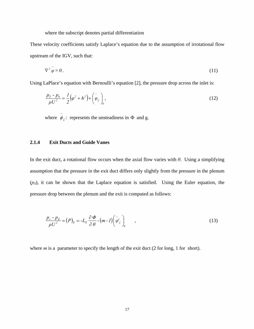
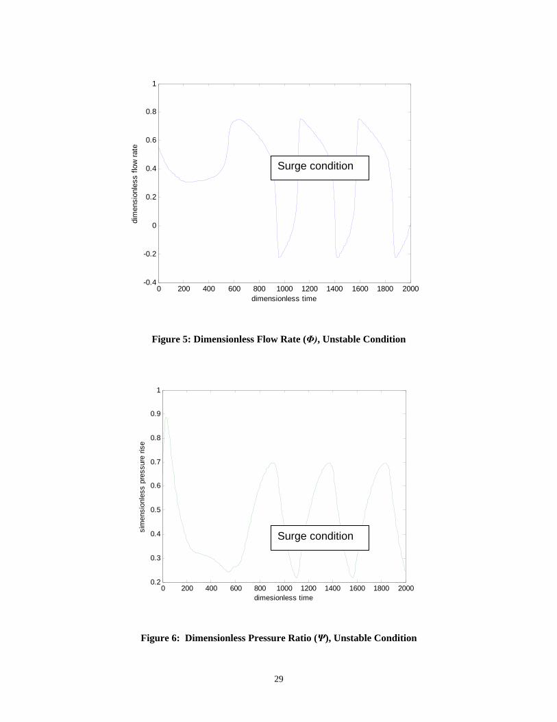
of the local maximum on the characteristic and, therefore in the surge condition. Figures 5-8
present the results of the simulation. Figure 5 gives the dimensionless flow rate, Figure 6 gives
the dimensionless pressure ratio, Figure 7 gives the rotating stall coefficient, and Figure 8 gives
the dimensionless compressor speed.
29
0 200 400 600 800 1000 1200 1400 1600 1800 2000-0.4
-0.2
0
0.2
0.4
0.6
0.8
1
dimensionless time
dim
ensi
onle
ss fl
ow ra
te
Figure 5: Dimensionless Flow Rate (Φ), Unstable Condition
0 200 400 600 800 1000 1200 1400 1600 1800 20000.2
0.3
0.4
0.5
0.6
0.7
0.8
0.9
1
dimesionless time
sim
ensi
onle
ss p
ress
ure
rise
Figure 6: Dimensionless Pressure Ratio (Ψ), Unstable Condition
Surge condition
Surge condition

30
0 200 400 600 800 1000 1200 1400 1600 1800 2000-0.5
0
0.5
1
1.5
2
2.5
3
3.5
4
dimesionless time
rota
ting
stal
l coe
ffici
ent
Figure 7: Stall Coefficient (J), Unstable Condition
0 200 400 600 800 1000 1200 1400 1600 1800 20000
0.5
1
1.5
2
2.5
dimesionless time
dim
ensi
onle
ss c
ompr
esso
r spe
ed
Figure 8: Dimensionless Compressor Speed (B), Unstable Condition
Rotating stall condition
Slight speed oscillation due to surge

31
As shown from Figure 7, the compressor starts in a rotating stall position since the J value is
greater than zero. The pressure (Figure 6) is decreasing at this stage, however the flow rate
(Figure 5) is staying relatively constant. This is due to the fact that even though individual
compressor blades are experiencing reduced flow, the average flow around the entire compressor
is constant. As the time increases the input torque begins to increase the speed of the compressor
due to the proportional control algorithm (Figure 8). As the speed increases, the stall is damped
out and the compressor goes into axial surge. This can be seen by the oscillating flow rate and
pressure starting around ξ = 600 on the abscissa. Figure 5 shows the flow rate dropping below
zero which implies that the flow is actually reversing through the compressor. This is consistent
with the definition of surge in a compressor and shows that the model can simulate both unstable
conditions. The results in Figures 5-8 match those reported in [3].
The second simulation discussed in [3] is a stable condition. This displays the model starting in
rotating stall and recovering to steady state equilibrium. The throttle coefficient ( γ ) is set to
0.65 and the proportional gain, P, is set to 2. Figures 9-12 are similar to Figures 5-8
respectively.

32
0 200 400 600 800 1000 1200 1400 1600 1800 20000.4
0.45
0.5
0.55
0.6
0.65
0.7
0.75
0.8
dimesionless time
dim
ensi
onle
ss fl
ow ra
te
Figure 9: Dimensionless Flow Rate (Φ), Stable Condition
0 200 400 600 800 1000 1200 1400 1600 1800 20000.1
0.2
0.3
0.4
0.5
0.6
0.7
0.8
dimesionless time
dim
esni
oles
s pr
essu
re ra
tio
Figure 10: Dimensionless Pressure Ratio (Ψ), Stable Condition
Steady state condition
Steady state condition

33
0 200 400 600 800 1000 1200 1400 1600 1800 2000-0.2
0
0.2
0.4
0.6
0.8
1
1.2
1.4
dimesionless time
rota
ting
stal
l coe
ffici
ent
Figure 11: Stall Coefficient (J), Stable Condition
0 200 400 600 800 1000 1200 1400 1600 1800 20000
0.5
1
1.5
2
2.5
dimesionless time
dim
ensi
onle
ss c
ompr
esso
r spe
ed (B
)
Figure 12: Dimensionless Compressor Speed (B), Stable Condition
Steady state condition

34
As shown in figures 9-12, the compressor enters rotating stall at the onset of the simulation (ξ =
200) when the speed (B) is low. This can be seen by the positive stall coefficient (J) in Figure
11. As the input torque gain increases and the compressor gets up to speed, the stall damps out
and the compressor enters a steady state condition. Flow rate, speed, and pressure rise all
stabilize to a constant value with the stall coefficient at zero. Therefore, the model can simulate
a recovery from a stalled condition as well as a steady state condition. These results duplicate
those given in [3] and provide confidence that the compressor model is sufficient for
incorporation into the entire power plant model.
It was desired to be able to simulate and study the entire model in Simulink. This will allow a
more thorough means for a control study and an intuitive feel for the complete model itself.
However, due to the complexity of the compressor model, it would be difficult to simulate in
Simulink using the standard library of tools. Therefore, a custom Simulink block called an S-
function was created. Simulink uses these functions to call lower functions to simulate the block
and incorporate it with other Simulink blocks. The S-function uses a set of coupled nonlinear 1st
order ODE’s that can be solved numerically. The following model is used:
⎥⎥⎥⎥
⎦
⎤
⎢⎢⎢⎢
⎣
⎡
=
JBΨΦ
y (48)
)y(f]y[ =& (49)
where f - the non-linear compressor model described above
y - output

35
The controller was again based on a proportional (P) type controller used previously. However
this is broken out of the model and used as the input in a feedback loop. This P type controller
could be replaced with a PID or more advanced control algorithm (to be studied later). Figure 13
shows the Simulink model for the compressor:
.5
gamma
Scope
f(u)
P-type Control ler
mcomp_s_function
Comp S Function
Figure 13: Simulink Model of Axial Flow Compressor
The function in the P-type controller is:
])3[u*bU(c d - ,
where c is the proportional gain,
b = p
ccs V
LAa2 , (50)
and u[3] is the third state variable in the vector output of the s-function (B).
The model was simulated using the above parameters for stable and unstable conditions to verify
the results (Figures 14 - 21):

36
0 200 400 600 800 1000 1200 1400 1600 1800 2000-0.4
-0.2
0
0.2
0.4
0.6
0.8
1
Dimensionless Time
Dim
ensi
onle
ss F
low
Rat
e
Figure 14: Simulink Compressor Model Results, Flow Rate (Φ), Unstable Condition
0 200 400 600 800 1000 1200 1400 1600 1800 20000.1
0.2
0.3
0.4
0.5
0.6
0.7
0.8
0.9
Dimensionless Time
Dim
ensi
onle
ss P
ress
ure
Ris
e
Figure 15: Simulink Compressor Model Results, Pressure Ratio (Ψ), Unstable Condition

37
0 200 400 600 800 1000 1200 1400 1600 1800 20000
0.5
1
1.5
2
2.5
Dimensionless Time
Dim
ensi
onle
ss C
ompr
esso
r Spe
ed
Figure 16: Simulink Compressor Model Results, Compressor Speed (B), Unstable Condition
0 200 400 600 800 1000 1200 1400 1600 1800 2000-0.5
0
0.5
1
1.5
2
2.5
3
3.5
4
Dimensionless Time
Dim
ensi
onle
ss S
tall
Coe
ffici
ent
Figure 17: Simulink Compressor Model Results, Stall Coefficient (J), Unstable Condition

38
0 200 400 600 800 1000 1200 1400 1600 1800 20000.4
0.45
0.5
0.55
0.6
0.65
0.7
0.75
0.8
Dimensionless Time
Dim
ensi
onle
ss F
low
Rat
e
Figure 18: Simulink Compressor Model Results, Flow Rate (Φ), Stable Condition
0 200 400 600 800 1000 1200 1400 1600 1800 20000.1
0.2
0.3
0.4
0.5
0.6
0.7
0.8
Dimensionless Time
Dim
ensi
onle
ss P
ress
ure
Ris
e
Figure 19: Simulink Compressor Model Results, Pressure Ratio (Ψ), Stable Condition

39
0 200 400 600 800 1000 1200 1400 1600 1800 20000
0.5
1
1.5
2
2.5
Dimensionless Time
Dim
ensi
onle
ss C
ompr
esso
r Spe
ed
Figure 20: Simulink Compressor Model Results, Compressor Speed (B), Stable Condition
0 200 400 600 800 1000 1200 1400 1600 1800 20000
0.2
0.4
0.6
0.8
1
1.2
1.4
Dimensionless Time
Dim
ensi
onle
ss S
tall
Coe
ffici
ent
Figure 21: Simulink Compressor Model Results, Stall Coefficient (J), Stable Condition

40
Comparing Figure 14 to Figures 5-8 and Figure 15 to Figures 9-12, the results of the s-function
match the script file and the results quoted in [3].
2.2 COMBUSTOR
Combustors are typically used in gas turbine cycles to heat the working fluid between the
compressor and the turbine. This process increases the enthalpy and temperature of the working
fluid. This additional energy is then extracted by the turbine. This is why the turbine can
produce more power than it takes to run the compressor and is the source of the net power output
of the entire gas turbine power plant. Figure 22 shows the location of the combustor in a typical
gas turbine system. Figure 23 shows the temperature – entropy (s) diagram of a typical gas
turbine cycle with respect to the different locations of the working fluid (a, b, c, d). The section
of the graph between b and c is the combustor section. The rise in temperature and entropy (and
enthalpy) provides the additional energy to the fluid to be extracted by the turbine. Without the
combustor, or some form of heat addition to the fluid, the turbine would simply produce enough
energy to run the compressor and no additional energy would be created. From a conservation of
energy viewpoint, the additional heat energy (or chemical energy of the fuel) is converted to
mechanical energy by the turbine [6].

41
Figure 22: Typical Gas Turbine Cycle
Figure 23: Temperature – Entropy Diagram of Typical Gas Turbine Cycle
42
2.2.1 Combustor Model
A simple combustor model is needed to incorporate into the overall fuel cell – gas turbine
system. The model must be able to simulate the temperature rise to the working fluid when it is
combusted with the compressed air exiting the compressor. The model assumes the fuel input to
the combustor to be methane. However, it is possible to burn the excess hydrogen straight from
the fuel cell output. This information will then be used to calculate the power extracted by the
turbine as well as the speed of the compressor and turbine shaft (they are rigidly connected) and
the torque on the turbine.
The combustor model used was developed by Fannin [5]. It is called an “unsteady well stirred
reactor” (WSR) model. It assumes methane (CH4) as the fuel and air as the oxidizer. The
balanced combustion reaction is as follows:
222224 N52.7OH2CO)N76.3O(2CH ++ ⇒++ (51)
A non-linear state space model can be constructed using conservation of species and energy in
the control volume of the combustor. The conservation of species equations are based on the
three species present inside the combustor. They are the fuel (methane), the oxidizer (air), and
the products of combustion. A conservation equation can be written for each species in terms of
the mass fractions inside the control volume:
productsoxidfuel
fuelfuel mmm
mY
++= (52)

43
productsoxidfuel
oxidoxid mmm
mY
++= (53)
productsoxidfuel
prodprod mmm
mY
++= (54)
where Yfuel, Yoxid, Yprod – mass fraction of fuel, oxidizer, and products inside the
combustor
mfuel, moxid, mprod – mass of fuel, oxidizer, and products inside the control volume
In words, the conservation of species equation is stated: The change in the amount of species in
the control volume is equal to the amount of species in, minus the amount of species out, plus the
amount of species created. For the oxidizer and fuel, the amount created inside the control
volume will be negative. For the products of combustion, the amount of species created will be
positive. This can be visualized by Figure 24.
COMBUSTOR
FUEL IN
OXIDIZER IN
FUEL INSIDE
OXIDIZER INSIDE
PRODUCTS INSIDE
FUEL OUT
OXIDIZER OUT
PRODUCTS OUT
Figure 24: Conservation of Species of Combustor

44
The amount of species created in the control volume will be driven by the Arrhenius rate term
for chemical kinetics of combustion. The conservation of species equations for the fuel and
oxidizer are as follows:
V)t(ωMW)t(Ym)t(Ymdt
)t(dYVρ fuelfuelfueloutin,fuelin
fuel&&& +-= (55)
V)t(ω)t(Y)t(Y
MW)t(Ym)t(Ymdt
)t(dYVρ fuel
in,fuel
in,oxidfueloxidoutin,oxidin
oxid &&& +-= (56)
where
( ) )t(TR098,15
3.1oxid
3.0fuelfuel
ueY233.0Yρs*kg
kmol100,24ω - ⎟⎟⎠
⎞⎜⎜⎝
⎛=& (57)
and ρ – density inside combustor
V – volume of combustor
inm& - total mass flow rate into combustor
Yfuel,in, Yoxid,in - mass fraction of fuel & oxidizer into combustor respectively
outm& - total mass flow rate out of combustor
MWfuel – molecular weight of fuel (methane)
fuelω& - Arrhenius rate term for consumption of species due to combustion
Due to the definition of the mass fraction, the equation for the mass fraction of the products is
simply
Yprod = 1 - Yfuel - Yoxid, (58)

45
and is not a differential equation. The state variables of the system to this point are Yfuel and Yoxid.
The third state variable will be temperature and is described by the energy equation.
The conservation of energy equation completes the model and is described as the amount of
energy entering the combustor minus the amount of energy leaving the combustor balanced by a
storage term.
∑ ∑-3
1i
3
1iout,iioutin,fuelin,fuelin,oxidin,oxidinii )t(h)t(Ym)hYhY(m)t(e)t(Y
dtdVρ
= =
+= && (59)
where ei – specific internal energy for i = 1-fuel, 2-oxidizer, 3-products
hoxid,in, hfuel,in – specific enthalpy of oxidizer and fuel into the combustor
hi,out – specific enthalpy for i = 1-fuel, 2-oxidizer, 3-products out of combustor
The right side of equation (59) is the total change in internal energy of the three species inside
the combustor. The left hand side is the energy associated with the enthalpy of the input species
and output species. All of these quantities are dependent on temperature, which is the desired
output variable from the combustor model. Therefore, equation (59) is converted to be in terms
of temperature rather than internal energy and enthalpy.
As stated above, the left hand side of equation (59) represents the change in internal energy of
the species inside the combustion chamber. In order to make this term an expression of
temperature only (and not Yfuel, and Yoxid) it is assumed that the majority of the species inside the
combustor are products (CO2, H2O, and N2), such that:

46
∑=
-+=3
1iout,iioutin,fuelin,fuelin,oxidin,oxidinprod )t(h)t(Ym)hYhY(m)t(e
dtd
Vρ && (60)
A linear curve fit based on the ideal gas properties of the products can be approximated, giving a
relationship between the specific internal energy and the temperature of the combustor products.
This same technique can be applied to the enthalpy terms on the right side of equation (59).
Therefore, equation (59) can be analyzed in terms of temperature (T) as a function of time. This
will be the third state variable and will complete the combustor model.
The linear curve-fits of the internal energy and enthalpy data are shown in Figures 25 and 26.
The actual data was obtained from ideal gas tables [6]. A linear equation was fit to the data.
These equations will be incorporated into equation (60) to obtain a state equation for
temperature. The enthalpy and internal energy of the products can be obtained by summing each
of the contributions of the product species on a mass fraction basis. The mass fractions of the
product species (CO2, H2O, and N2) can be obtained using the stiochiometry in equation (51)
along with their respective molecular masses.

47
Specific Internal Energy Curve Fits
y = 532.35x - 946.55
y = 272.3x - 489.1
y = 232.21x - 333.11
-1000
0
1000
2000
3000
4000
5000
6000
7000
8000
0 250 500 750 1000 1250 1500 1750 2000 2250 2500 2750 3000 3250
Temperature (K)
Inte
rnal
Ene
rgy
(kJ/
kg)
CO2H2ON2Linear (H2O)Linear (CO2)Linear (N2)
Figure 25: Linear Curve Fit of Internal Energy of Products
Specific Enthalpy (kJ/kg)
y = 647.7x - 1061.9
y = 306.41x - 407.32
y = 319.53x - 536.3
y = 286.07x - 343.47
-1000
0
1000
2000
3000
4000
5000
6000
7000
8000
9000
0 250 500 750 1000 1250 1500 1750 2000 2250 2500 2750 3000 3250
Temperature (K)
Ent
halp
y (k
J/km
ol)
CO2H2ON2AirLinear (H2O)Linear (N2)Linear (CO2)Linear (Air)
Figure 26: Linear Curve Fit of Enthalpy of Products and Air

48
The enthalpy equation used in the model for the fuel (methane) is as follows:
Tchh pffuel += (61)
where hf - enthalpy of formation
cp,fuel - constant pressure specific heat
Equation (60) then becomes (61)
)]Tch)(t(Y)t(h)t(Y[m)hYhY(m)t(edtd
Vρ fuel,p11
3
2iout,iioutin,fuelin,fuelin,oxidin,oxidinprod ++-+= ∑
=
&& (61)
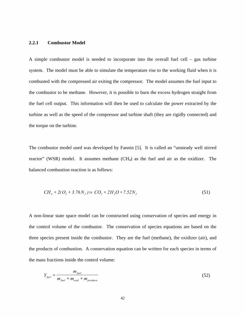
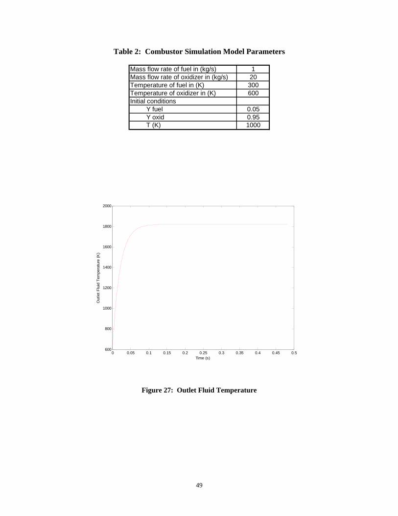
2.2.2 Combustor Model Simulation
A script file was written in MATLAB to simulate the model. The results are displayed in
Figures 27 – 29. The outputs of the system are the combustor temperature (Figure 27), which is
assumed to be the exit flow temperature, and the mass fractions of the fuel and oxidizer inside
the combustor (Figures 28 and 29, respectively). This simulation uses constant fuel and oxidizer
input flow rates. The parameters of the simulation are summarized in Table 1. The air to fuel
mass ratio is close to the stoichiometric value of 17.123.
49
Table 2: Combustor Simulation Model Parameters
Mass flow rate of fuel in (kg/s) 1Mass flow rate of oxidizer in (kg/s) 20Temperature of fuel in (K) 300Temperature of oxidizer in (K) 600Initial conditions
Y fuel 0.05Y oxid 0.95T (K) 1000
0 0.05 0.1 0.15 0.2 0.25 0.3 0.35 0.4 0.45 0.5600
800
1000
1200
1400
1600
1800
2000
Time (s)
Out
let F
luid
Tem
pera
ture
(K)
Figure 27: Outlet Fluid Temperature

50
0 1 2 3 4 5 6 7
x 10-6
-0.1
-0.05
0
0.05
0.1
0.15
0.2
0.25
0.3
Time (s)
Fuel
Mas
s R
atio
Figure 28: Fuel Mass Fraction Inside Combustor
0 0.5 1 1.5 2 2.5 3 3.5 4 4.5
x 10-4
-1
-0.5
0
0.5
1
1.5
2
2.5
3
x 10-3
Time (s)
Oxi
dize
r Mas
s R
atio
Figure 29: Oxidizer Mass Fraction Inside Combustor

51
As can be observed from Figure 21, the combustor raises the temperature of the working fluid
from 600K to approximately 1800K. These results are consistent with the test data provided in
[5]. The mass fractions of the fuel and the oxidizer fall rapidly and eventually stabilize near
zero. This result implies that nearly all of the fuel and the oxidizer are being converted to
products, which is consistent with the ratio of the fuel and oxidizer, which was chosen to be
close to the stoichiometric value. The value of the product mass fraction inside the combustor
would be close to unity according to equation (58). This gives credence to the assumption that
the exit fluid consists of mostly products of combustion.
A Simulink model was created based on the script file discussed above. It uses a user defined s-
function [15] to simulate the combustor model (Figure 30). The inputs are the same as the above
model but the outputs have been changed to reflect the mass flow rate out of the combustor along
with the temperature of those products (63).
total,outtotal,inoxidfuel,in mmmm &&&& ==+ (63)

52
30
mdot_oxid_in (kg/s)
1
mdot_fuel_in (kg/s)Scope
combustor2_s_function
S-Function
em
Figure 30: Combustor Model in Simulink Using S-Function
By running the same simulation parameters as above, the temperature of the exit products can be
duplicated using the simulink model (Figures 31, 32). The mass flow rate of the exit products is
a simple algebraic relation (63), and can be verified by inspection. This result gives confidence
to the s-function representing the model described in [5].
0 0.05 0.1 0.15 0.2 0.25600
800
1000
1200
1400
1600
1800
2000
time (s)
Out
put P
rodu
cts
Tem
pera
ture
(K)
Figure 31: Output Temperature of Simulink Combustor Model
53
0 0.05 0.1 0.15 0.2 0.2530
30.2
30.4
30.6
30.8
31
31.2
31.4
31.6
31.8
32
time (s)
Mas
s Fl
ow R
ate
of P
rodu
cts
(kg/
s)
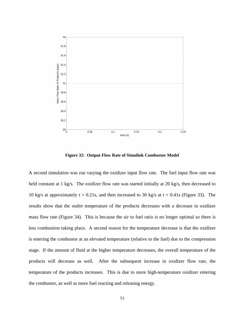
Figure 32: Output Flow Rate of Simulink Combustor Model
A second simulation was run varying the oxidizer input flow rate. The fuel input flow rate was
held constant at 1 kg/s. The oxidizer flow rate was started initially at 20 kg/s, then decreased to
10 kg/s at approximately t = 0.21s, and then increased to 30 kg/s at t = 0.41s (Figure 33). The
results show that the outlet temperature of the products decreases with a decrease in oxidizer
mass flow rate (Figure 34). This is because the air to fuel ratio is no longer optimal so there is
less combustion taking place. A second reason for the temperature decrease is that the oxidizer
is entering the combustor at an elevated temperature (relative to the fuel) due to the compression
stage. If the amount of fluid at the higher temperature decreases, the overall temperature of the
products will decrease as well. After the subsequent increase in oxidizer flow rate, the
temperature of the products increases. This is due to more high-temperature oxidizer entering
the combustor, as well as more fuel reacting and releasing energy.

54
0 0.05 0.1 0.15 0.2 0.25 0.3 0.35 0.4 0.45 0.510
15
20
25
30
35
time (s)
Mas
s Fl
ow R
ate
of P
rodu
cts
(kg/
s)
Figure 33: Mass Flow Rate of Combustor Model with Varying Input Air Flow Rate
0 0.05 0.1 0.15 0.2 0.25 0.3 0.35 0.4 0.45 0.5600
800
1000
1200
1400
1600
1800
2000
time (s)
Out
put P
rodu
cts
Tem
pera
ture
(K)
Figure 34: Output Temperature of Simulink Combustor Model with Varying Oxidizer Input Flow Rate

55
2.3 TURBINE
2.3.1 Turbine Theory
The turbine model is needed to simulate the torque imparted to the compressor and the generator
as well as to determine the portion of the overall power developed by the gas turbine. Torque is
developed in the turbine when the working fluid expands and imparts a force on the turbine
blades (Figure 35). The working fluid enters the turbine stator with a velocity CT1 and exits it
with a velocity of CT2. When the fluid passes through the turbine rotor stage, the change in
direction of the fluid to CT3 imparts a force on the rotor, which provides the torque to the
compressor and the generator and rotates the rotor with a velocity U. Unlike the compressor
model, turbines are relatively stable and do not suffer from surge. This is because the pressure
drop is in the same direction of the flow of the working fluid. Therefore there is no force to
reverse the flow as in the compressor [6], [14].

56
CT1
CT2
CT3
U Rotor
Stator
Figure 35: Example Turbine Stage
2.3.2 Turbine Function
The turbine model used here will actually be an algebraic function rather that a state space
differential model. This is because the actual rotor dynamics are encompassed in the compressor
model developed above (equations (34) – (42)). Since the compressor and the turbine are rigidly
coupled, the speed of the turbine is extracted from the compressor model. The compressor
model uses the turbine torque to calculate the speed of the rotor based on the rotational
momentum balance (34).
The power developed by the turbine is calculated using the change in enthalpy in the working
fluid. This enthalpy is based on the linearized enthalpy temperature relationship of the products
of combustion developed for the combustor model (Figure 26) [6].

57
)hh(mηP outininTturb -= & (64)
where Pturb – total power developed by the turbine
inm& - total mass flow rate into the turbine
ηT - isentropic efficiency of turbine
hin – total specific enthalpy of the working fluid into the turbine
hout – total specific enthalpy of the working fluid out of the turbine based on room
temperature
The torque developed by the turbine can be calculated using the power developed by the turbine
and the angular velocity of the rotor from the compressor model.
ωP
τ turbt = (65)
where tτ – total torque developed by the turbine
tτ is fed into the compressor model to determine ω . The net torque out of the entire gas turbine
is calculated using the difference between tτ and cτ .
ctnet τττ -= (66)
where netτ - the available torque to run the generator.
58
Therefore the net power out of the gas turbine is:
ωτP netout = (67)
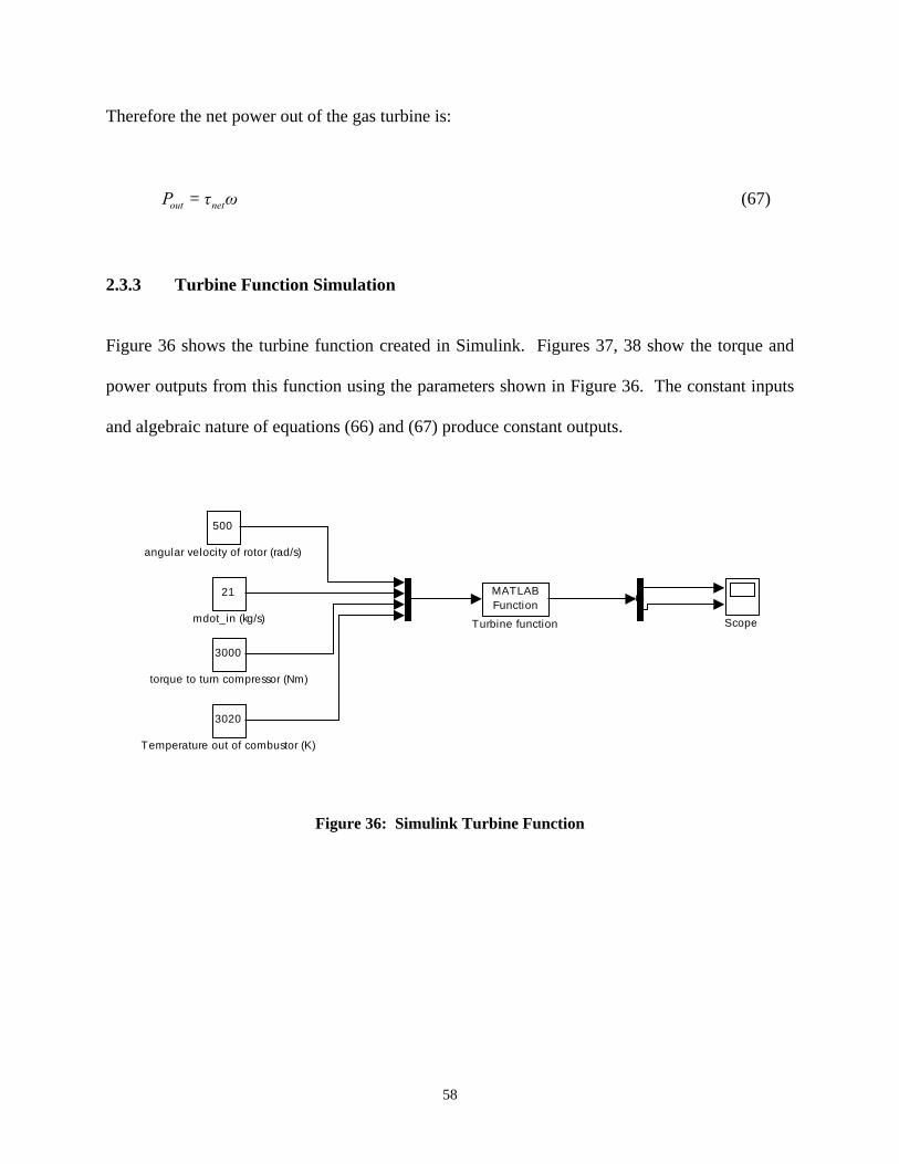
2.3.3 Turbine Function Simulation
Figure 36 shows the turbine function created in Simulink. Figures 37, 38 show the torque and
power outputs from this function using the parameters shown in Figure 36. The constant inputs
and algebraic nature of equations (66) and (67) produce constant outputs.
3000
torque to turn compressor (Nm)
21
mdot_in (kg/s)
500
angular velocity of rotor (rad/s)
MATLABFunction
Turbine function
3020
Temperature out of combustor (K)
Scope
em
Figure 36: Simulink Turbine Function

59
0 1 2 3 4 5 6 7 8 9 101.0288
1.0289
1.0289
1.029
1.029
1.0291x 10
4
time (s)
Turb
ine
Torq
ue G
ener
ated
(Nm
)
Figure 37: Turbine Torque Generated from Uncoupled Turbine Simulation
0 1 2 3 4 5 6 7 8 9 103.6446
3.6446
3.6446
3.6446
3.6446
3.6446
3.6446
3.6446
3.6446
3.6446
3.6446x 10⁶
time (s)
Net
Pow
er O
ut (W
)
Figure 38: Net Power Out from Uncoupled Turbine Simulation
60
3.0 HEAT EXCHANGER AND FUEL CELL MODELS
The following sections will develop the dynamic heat exchanger and fuel cell models. These
models will complete the components needed to create a FCGT hybrid power plant model.
3.1 HEAT EXCHANGER
3.1.1 Heat Exchanger Theory
A heat exchanger model will be needed to transfer the energy of the hot fuel cell fluids to the
working fluid of the gas turbine. The heat exchangers can be used in various places throughout
the power plant. Counter flow design is chosen, which means that the hot and cold streams flow
in opposite directions through the heat exchanger. This allows the outlet temperature of the cold
fluid to exceed the outlet temperature of the hot fluid (Figure 39). This is not possible in parallel
flow heat exchangers. Counter flow heat exchangers are also more efficient in that they can
transfer the same amount of energy between flows with a smaller surface area [7].
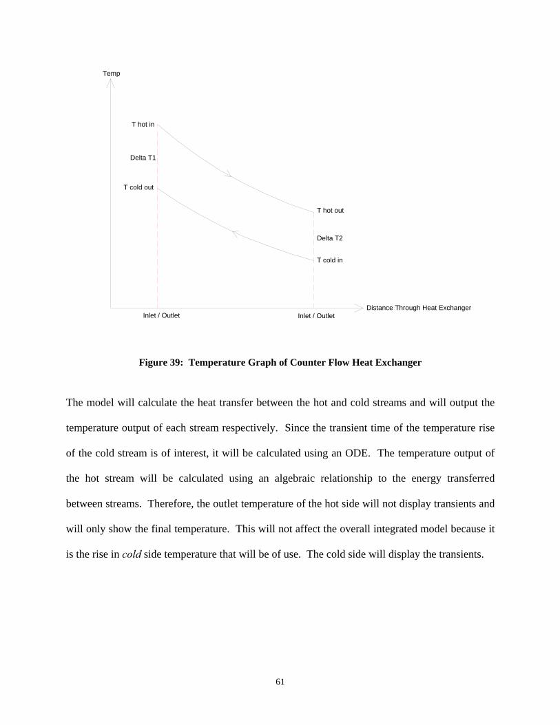
61
Temp
Distance Through Heat Exchanger
T hot in
T hot out
T cold in
T cold out
Inlet / Outlet Inlet / Outlet
Delta T1
Delta T2
Figure 39: Temperature Graph of Counter Flow Heat Exchanger
The model will calculate the heat transfer between the hot and cold streams and will output the
temperature output of each stream respectively. Since the transient time of the temperature rise
of the cold stream is of interest, it will be calculated using an ODE. The temperature output of
the hot stream will be calculated using an algebraic relationship to the energy transferred
between streams. Therefore, the outlet temperature of the hot side will not display transients and
will only show the final temperature. This will not affect the overall integrated model because it
is the rise in cold side temperature that will be of use. The cold side will display the transients.

62
3.1.2 Heat Exchanger model
The following is a list of assumptions used in the heat exchanger model:
• Laminar flow
• Pressure drop through the heat exchanger (HX) is negligible
• The temperature of the cold stream equals the temperature of the HX metal
• Log mean temperature profile - Equation (68) [7]
• Both hot and cold fluids are air
)T∆/T∆ln(T∆T∆
T∆21
21lm
-= (68)
where lmT∆ - log mean temp. difference of hot and cold streams
o,ci,h1 TTT∆ -= (69)
i,co,h2 TTT∆ -= (70)
o,hi,h T,T - Temp. of inlet and outlet of hot stream
o,ci,c T,T - Temp. of inlet and outlet of cold stream
Parameters for the heat exchanger were derived from the flow rate vs. effectiveness information
given by Solar Turbines via the Department of Energy (DOE). The heat transfer is given by the
“ProTrax” equation [17]. The equation for the outlet temperature of the metal, which is assumed
to be the outlet temperature of the cold stream, is given by equation (71) [16]:
[ ]q)TT(CmCm1
tT
o,ci,ccold,pcoldmetal,pmetal
o,c += - d
d& (71)

63
where metalm - mass of the metal in the heat exchanger
metal,pC - specific heat of the heat exchanger metal
coldm& - mass flow rate of the cold stream
cold,pC - specific heat of the cold stream
q - rate of heat transfer between streams
The rate of heat transfer is calculated using the “ProTrax” equation [17]:
( )i,ci,h
cold,pcoldhot,phot
X
X
TT
Cm1
Cme
eq -
&&
= (72)
where hotm& - mass flow rate of the hot stream
hot,pC - specific heat of the hot stream
X – dimensionless parameter defined as
⎟⎟⎠
⎞⎜⎜⎝
⎛=
cold,pcoldhot,photHXbulk Cm
1Cm1AkX
&&- (73)
where kbulk – bulk thermal conductivity of the streams
AHX – HX surface area to gap provided by DOE
The temperature of the hot stream output is simply [7]:
hot,photi,ho,h Cm
qTT
&-= (74)

64
These equations comprise the heat exchanger model and will account for variations in the hot
and cold stream inlet temperatures and flow rates.
3.1.3 Heat Exchanger Model Simulation
An s-function was written in MATLAB to simulate the heat exchanger using Simulink (Figure
40). The parameters used for this simulation are summarized in Table 3.
Table 3: Heat Exchanger Simulation Parameters
mmetal 90 kg
coldm& 0.7 kg/s, 1kg/s
hotm& 0.7 kg/s
Tc,i 400 K
Th,i 800 K

65
.7
mdot_hot (kg/s)
.7
mdot_cold (kg/s)
800
T_hot_in (K)
400
T_cold_in (K)
Scope3
Scope2
Scope1
Scope
HeatEx_s_function
Heat Exchanger
em
Figure 40: Heat Exchanger Simulink S-Function
The specific heat values and thermal conductivities for the hot and cold streams are calculated
based on their respective temperatures [6]. Figures 41 - 44 show the outputs when the
parameters shown in Figure 40 are run on the model.
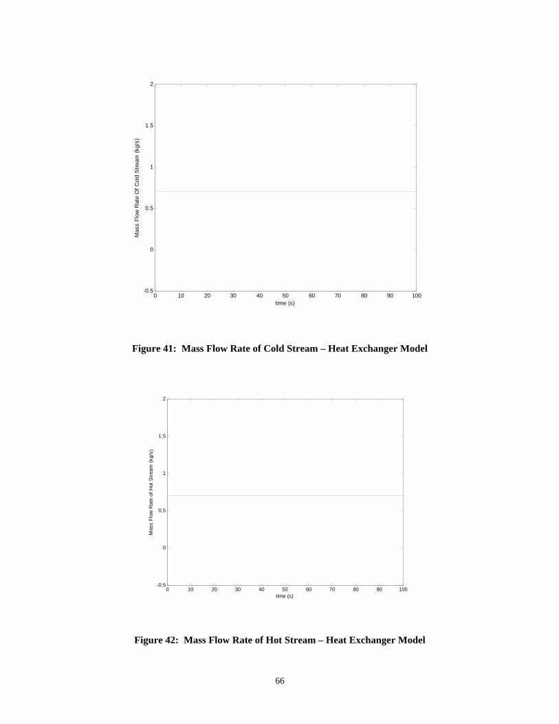
66
0 10 20 30 40 50 60 70 80 90 100-0.5
0
0.5
1
1.5
2
time (s)
Mas
s Fl
ow R
ate
Of C
old
Stre
am (k
g/s)
Figure 41: Mass Flow Rate of Cold Stream – Heat Exchanger Model
0 10 20 30 40 50 60 70 80 90 100-0.5
0
0.5
1
1.5
2
time (s)
Mas
s Fl
ow R
ate
of H
ot S
tream
(kg/
s)
Figure 42: Mass Flow Rate of Hot Stream – Heat Exchanger Model

67
0 10 20 30 40 50 60 70 80 90 100400
450
500
550
600
650
700
750
800
time (s)
Tem
pera
ture
Out
of C
old
Stre
am (K
)
Figure 43: Outlet Temperature of Cold Stream – Heat Exchanger Model
0 10 20 30 40 50 60 70 80 90 100436.5
437
437.5
438
438.5
439
time (s)
Tem
pera
ture
Out
of H
ot S
tream
(K)
Figure 44: Outlet Temperature of Hot Stream – Heat Exchanger Model

68
As shown from Figure 43, the outlet temperature of the cold stream gradually increases to a
steady state value of 775K while the cold and hot mass flows (Figures 41, 42) are kept constant.
The flow rates are taken directly from the inputs. The outlet temperature of the hot side (Figure
44) is constant as well due to the algebraic nature of the equations. However, as stated above, it
is the cold side that is of consequence in the integrated power plant model. Figures 45 - 48 show
the results of the model run with a slightly higher cold stream flow rate. The outlet temperature
of the cold stream is slightly lower than before. This is because the cold steam is not exposed to
the heat exchanger for as long. Therefore the energy transfer rate is lower and less heat is
transferred.
0 10 20 30 40 50 60 70 80 90 1000
0.2
0.4
0.6
0.8
1
1.2
1.4
1.6
1.8
2
time (s)
Mas
s Fl
ow R
ate
of C
old
Stre
am (k
g/s)
Figure 45: Mass Flow Rate of Cold Stream – Heat Exchanger Model with Higher Cold Mass Flow Rate

69
0 10 20 30 40 50 60 70 80 90 100-0.5
0
0.5
1
1.5
2
time (s)
Mas
s Fl
ow R
ate
of H
ot S
tream
(kg/
s)
Figure 46: Mass Flow Rate of Hot Stream – Heat Exchanger Model with Higher Cold Mass Flow Rate
0 10 20 30 40 50 60 70 80 90 100400
450
500
550
600
650
700
time (s)
Tem
pera
ture
Out
of C
old
Stre
am (K
)
Figure 47: Temperature Out of Cold Stream – Heat Exchanger Model with Higher Cold Mass Flow Rate

70
0 10 20 30 40 50 60 70 80 90 100401.5
402
402.5
403
403.5
404
time (s)
Tem
pera
ture
Out
of H
ot S
tream
(K)
Figure 48: Temperature Out of Hot Stream – Heat Exchanger Model with Higher Cold Mass Flow Rate
3.2 FUEL CELL
3.2.1 Fuel Cell Operating Theory
The fuel cell (FC) is the main power generation system in the power plant. There are several
types of fuel cells that could be integrated with a gas turbine, two of which are the molten
carbonate and the solid oxide varieties, which are most suitable due to their high operating
temperature. The high temperature of the fluids leaving the fuel cell is used to run the gas

71
turbine and create more electrical energy. A solid oxide fuel cell model was developed for this
study, the basic operation of which is shown in Figure 49.
Figure 49: Solid Oxide Fuel Cell
As shown in the figure, hydrogen fuel enters the anode and combines with oxygen ions to form
steam and four electrons. These electrons are forced through a load as electricity (power) and
enter the cathode to combine with oxygen to produce the oxygen ions that flow through the
electrolyte. The oxygen is provided by air. The excess air exits at elevated temperature and can
be used to run the gas turbine. The solid oxide runs at the highest operating temperature of all
the types of fuel cells. This eliminates the need for expensive catalysts and provides the
possibility of including a bottoming cycle [8].
72
3.2.2 Fuel Cell Model
The FC model is based on a model developed by Padulles, Ault, and McDonald [9]. It was
developed for dynamic power simulation of solid oxide fuel cells. The assumptions for the fuel
cell model are as follows:
• The gases are ideal
• The fuel cell is fed with hydrogen and air
• The electrode channels are small enough that the pressure drop across them is negligible
• The ratio of pressures between the inside and outside of the electrode channels is large
enough to assume choked flow
• The fuel cell temperature is stable
• The Nerst equation applies
• The losses are as follows
o Ohmic
o Activation
o Mass Transport
The model development begins with the flow equation for choked flow [9].
MKP
m
u
fc =&
(75)
where fcm& - mass flow rate
K - valve constant
Pu - pressure upstream (inside electrode channels)
M - molar mass of fluid

73
A utilization factor (Uf) is defined as the ratio of the amount of hydrogen that reacts with the
oxygen ions ( reacted,H,fc 2m& ) over the amount of hydrogen entering the anode ( in,H,fc 2
m& ).
in,H,fc
reacted,H,fcf
2
2
mm
U&
&= (76)
By considering that the molar flow of any gas through the valve is proportional to its partial
pressure, the following equations are derived [9]
2
22
2
HH
an
H
H KMK
pq
== (77)
OHOH
an
OH
OH
2
22
2 KMK
pq
== (78)
where OHH 22q,q - molar flow rates of hydrogen and water respectively
OHH 22p,p - partial pressures of hydrogen and water respectively
Kan - valve constant of the anode
OHH 22K,K - valve molar constants for hydrogen and water respectively
By substituting equations (76), (77), (78), equation (75) can be written as:
74
( )[ ]OHfHfanan
fc22
MUMU1KPm
+= -&
(79)
where Pan – the pressure inside the anode channel
The ideal gas law will be used to find the partial pressures of the gasses flowing through the
electrodes. This technique will be applied to all the gasses. Only hydrogen will be derived here.
RTnVp22 HanH = (80)
where Van – volume of the anode channel
R – ideal gas constant
T – temperature
2Hn - moles of hydrogen in the channel
By isolating the pressure and taking the first time derivative, we have:
an
HH
VRTq
dtdp
22 = (81)
The hydrogen flow can be broken down to three parts and equation (81) can be rewritten as
follows
( )rH
outH
inH
an
H222
2 qqqVRT
dtdp
--= (82)

75
where inH 2
q - molar flow of hydrogen into the channel
outH 2
q - molar flow of hydrogen out of the channel
rH 2
q - molar flow of hydrogen that reacts in the channel
According to the electrochemical relationships, the amount of hydrogen that reacts can be
calculated by:
IK2F2IN
q r0r
H2== (83)
where N0 – number of cells in the stack series
F – Faraday’s constant
I – stack current
Kr – modeling constant
By substituting equations (83) and (77) into equation (82), taking the Laplace transform, and
isolating the partial pressure term, the following equation can be derived:
( )IK2qsτ1
K/1p r
inH
H
HH 2
2
2
2-
+= (84)
where 2Hτ - the system pole associated with the hydrogen flow

76
The stack output voltage is described by the Nerst equation [8]. The -rI term is the ohmis loss.
This is the loss due to the resistance of the electrodes and the resistance of the flow of O-2 ions
through the electrolyte.
rIp
ppln
F2RTENV
OH
5.0OH
002
22 -⎥⎥⎦
⎤
⎢⎢⎣
⎡⎟⎟⎠
⎞⎜⎜⎝
⎛+= (85)
where V - fuel cell output voltage
E0 - open cell voltage (based on the Gibbs free energy)
r - ohmic losses of the stack
The activation loss is caused by the sluggishness of the reactions at the electrode surfaces. A
portion of the voltage is lost in driving the chemical reaction that moves the electrons to the
electrodes. A way to account for these losses is to use the Tafel equation [8]. This equation was
derived by physical experimentation on various electrochemical reactions. It provides a
relationship between the overvoltage at the surface of an electrode and the log of the current
density. This can be used to calculate the activation voltage loss for a SOFC.
)iln(AV∆ act -= (86)
where actV∆ - activation voltage loss
A - slope of Tafel line (constant specific for SOFC)
i - current density (current / electrode area)

77
Mass transport losses are losses that occur due to the difference in concentration of the fuel as it
passes through the electrode. The concentration will be high when the fuel and air enter the
electrodes, but as they travel through, they get used in the reaction. This concentration affects
the partial pressure of the reactants and has an effect on the voltage that that portion of the
electrode can produce. Unfortunately this loss cannot be accurately calculated analytically.
Therefore, experimental results are used to empirically estimate the loss. Equation (87) has been
developed based on experiments and is accepted as a good approximation of the mass transport
losses [8].
)ni(trans meV∆ = (87)
where transV∆ - voltage loss due to mass transfer and concentration loss
m, n – constants derived from experiment (specific to SOFC)
Combining all the losses into equation (85) gives an equation for the overall voltage of a single
fuel cell. In an actual fuel cell power plant, multiple cells would be combined in series to
provide the necessary voltage and current demand [8]. The total stack voltage is:
)ni(
OH
5.0OH
00 me)iln(ArIp
ppln
F2RTENV
2
22 +⎥⎥⎦
⎤
⎢⎢⎣
⎡⎟⎟⎠
⎞⎜⎜⎝
⎛+= -- (88)
The total power generated from the FC (PFC) is simply:

78
VINP 0FC = (89)
3.2.3 Fuel Cell Model Simulation
A Simulink model was created to simulate the fuel cell based on the analysis performed above
(Figure 50). The model was run using parameters shown in Figures 50 and 51. Figures 52 and
53 show the voltage and power outputs of the model, respectively. The initial transients are due
to the startup of the model and the initial conditions of the transfer functions being zero. It can
be seen that the fuel cell produces approximately 200 kW of power with a 300 amp current
demand at steady state. The model uses 20 fuel cells connected in series. The parameters used
in the simulation are summarized in Table 4.
Table 4: Fuel Cell Simulation Parameters
Kr 9.95e-4 FC Temp 1273.15 K
kmol/kg_air 1/29 Kmol / kg_H2 1/2
N0 20 KH2 8.43e-4 kmol/(atm s) KH2O 2.81e-4 kmol/(atm s) KO2 2.52e-3 kmol/(atm s)
2Hτ 26.1 s
O2Hτ 78.3 s
2Oτ 2.91 s r 0.126 ohms

79
2Power
1Voltage
-K-
r (ohms)
20
number of cells in stack
.21
mol fraction of O2 in air
8e-4
mass transfer constant n (m^2/A)
1e-4
mass transfer const m (V)
-K-
kmol/kg_air
1/2
kmol/kg_H2
V*I
.002
Slope of Tafel l ine (V)
.5
Reaction Area of FC (m^2)
8314
R (J/kmol K)
.92
Open Cell Voltage (V)
1/2.52e-3
2.91s+1O2 Transfer Function
f(u)
Nerst equation
f(u)
Mass Transport loss (V)
-K-
Kr (kmol/s A)
1/2.81e-4
78.3s+1H2O transfer Function
1/8.43e-4
26.1s+1H2 Transfer Function
96485
Faraday's Const (C)
-C-
FC Temp (K)
Current Density (A/m^2)f(u)
Activation Loss (V)
-K-
2*Kr (kmol/s A)
#*V series
3m_dot air in (kg/s)
2m_dot H2 in (kg/s)
1Current (A)
Ohmis Loss (V)
Figure 50: Simulink Fuel Cell Model

80
Scope2
Scope1
Current (A)
m_dot H2 in (kg/s)
m_dot air in (kg/s)
Voltage
Power
Fuel Cel l
1
Constant2
.004
Constant1
300
Constant
Figure 51: Fuel Cell Simulation Parameters
0 100 200 300 400 500 600 700 800 900 1000-4000
-3000
-2000
-1000
0
1000
2000
time (s)
Tota
l Fue
l Cel
l Vol
tage
(V)
Figure 52: Fuel Cell Voltage

81
0 100 200 300 400 500 600 700 800 900 1000-10
-8
-6
-4
-2
0
2
4
6x 10⁵
time (s)
Tota
l Fue
l Cel
l Pow
er (W
)
Figure 53: Fuel Cell Power
A second simulation was run using a linear current ramp starting at 10 amps with a slope of 1.
Figure 54 shows the voltage response of the fuel cell. Initially, the voltage is low until the
current reaches a relatively high level. This is due to the transfer functions initial conditions of
zero. The voltage reached a peak just past 400 s after which it starts to drop. This is typical with
fuel cells and has to do with the irreversibilities when the current reaches a certain level [8].

82
0 100 200 300 400 500 600 700 8000
0.5
1
1.5
2
2.5
3x 10⁵
time (s)
Fuel
Cel
l Vol
tage
(V)
Figure 54: Fuel Cell Voltage Response Due to Linear Current Ramp

83
4.0 MODEL INTEGRATION
The models described above can be integrated into a number of combinations of fuel cell gas
turbine power plants [13], [18], [19], [21]. The basic idea is to combine them in such a way that
the high temperature of the fuel cell gases is exploited to run the gas turbine. This can be
accomplished with heat exchangers or running the same fluid through the fuel cell and the gas
turbine.
4.1 GAS TURBINE INTEGRATION
4.1.1 Gas Turbine Model Integration
The first step in integrating the individual component models is to construct a simple gas turbine
model. This entails combining the compressor, combustor, and turbine into a system that
produces a net power output. The integration of the gas turbine model is shown in Figure 22 and
the thermodynamic cycle is shown above in Figure 23. By combining the Simulink models as
shown in Figure 22, a complete gas turbine model is constructed (Figure 55).

84
Turbine Torque Out (Nm)1
0
Turbine Torque Out (Nm)
angular v elocity of rotor (rad/s)
mdot_in (kg/s)
torque to turn compressor (Nm)
Temperature out of combustor (K)
Turbine Torque Out (Nm)
Net Gas Tubine Power Out (W)
Turbine
.5
Throttle Coef.
Temp into Turbine (K)1
0
Temp into Turbine (K)
Stal l Corfficient (dim less)1
0
Stal l Corfficient (dim less)
Pressure out of Compressor (Pa)1
0
Pressure out of Compressor (Pa)
0
Net Power Out (W)1
Net Power Out (W)
0
Mass Fow Rate into Combustor (kg/s)1
Mass Fow Rate into Combustor (kg/s)
.08
Mass Flow Rate of Fuel into Combustor (kg/s)
throttle coef (gamma)
turbine torque in (Nm)
mdot_compressor (kg/s)
pressure af ter comp (Pa)
angular v elocity (rad/s)
Stall Coef
Torque to turn Compressor (Nm)
Compressor
mdot_f uel_in (kg/s)
mdot_oxid_in (kg/s)
Temp of Products Out (K)
mdot out of combusor (kg/s)
Combustor 0
Angular Veloci ty of Rotor (rad/s)1
Angular Veloci ty of Rotor (rad/s)
Figure 55: Gas Turbine Simulink Model

85
As shown in Figure 55, the inputs to the gas turbine are mass flow rate of fuel into the combustor
and the throttle coefficient into the compressor model. The mass flow rate into the combustor
controls the amount of fuel that is reacting. This will control the temperature of the combustion
products entering the turbine. Since the power developed by the turbine is dependent on the
input temperature of the working fluid, this flow rate can be used as a gas turbine control
variable. The throttle coefficient can be thought of as a bleed air valve which can control the
pressure drop across the turbine stage. This valve could therefore be used to control the speed of
the rotor and therefore the power out of the gas turbine portion of the power plant. The outputs
of the compressor model are mass flow rate, pressure, rotor angular velocity, and stall
coefficient. The mass flow rate is then used as an input to the combustor and the angular
velocity is connected to the input of the turbine model. This will calculate the power output of
the turbine (equation (67)). The stall coefficient is used to determine if the compressor is in
rotating stall. If this value is above zero, the compressor is experiencing some level of rotating
stall. The temperature and flow rate out of the combustor is used to calculate the enthalpy rise of
the working fluid and the power out of the turbine. The torque developed by the turbine is fed
back into the input of the compressor model. As stated above, the torque balance of the turbine
and compressor are calculated in the compressor model.
4.1.2 Gas Turbine Model Simulation
The gas turbine model was run using a value of 0.5 kg/s for the fuel input mass flow rate of the
combustor and a value of 0.5 for the throttle coefficient [3]. The results are shown in Figures 56
– 58. Figure 56 shows that the power produced by the turbine ramps up to quasi-equilibrium in
the first few seconds of operation. This is due to the initial conditions of the system at startup.

86
After the turbine reaches approximately 125 kW, it stabilizes and remains relatively constant
throughout the simulation. Figure 57 shows that the angular velocity of the rotor is increasing
throughout the simulation. This is due to the torque generated by the turbine being higher than
the torque to balance the angular velocity of the rotor, therefore the rotor rotates faster. A
stabilization technique for the rotor angular velocity is to control the output torque of the turbine
by varying the input fuel mass flow rate of the combustor or to incorporate a cold air injection to
control the inlet temperature of the turbine (Figure 58).
0 10 20 30 40 50 60 70 80 90 1000.5
1
1.5
2
2.5
3
3.5x 10⁵
time (s)
Gas
Tur
bine
Pow
er (W
)
Figure 56: Gas Turbine Output Power

87
0 10 20 30 40 50 60 70 80 90 10096
96.5
97
97.5
98
98.5
99
99.5
100
time (s)
Rot
or A
ngul
ar V
eloc
ity (r
ad/s
)
Figure 57: Gas Turbine Rotor Angular Velocity
0 10 20 30 40 50 60 70 80 90 100600
800
1000
1200
1400
1600
1800
2000
time (s)
Turb
ine
Inle
t Tem
pera
ture
(K)
Figure 58: Turbine Inlet Temperature

88
4.2 FUEL CELL – GAS TURBINE
4.2.1 FCGT – Integration Configuration One
As stated above, there are several ways to combine a fuel cell and gas turbine into a hybrid
power plant. One of which is to run the fuel cell independently and use a heat exchanger to
transfer the heat from the fuel cell exhaust to the working fluid of the gas turbine after
compression and before expansion. This eliminates the need for a combustor to raise the
temperature of the working fluid before the turbine. This configuration is shown in Figure 59.
An advantage to completely separating the working fluids of the fuel cell and the gas turbine is
that the pressure fluctuations in the gas turbine won’t affect the pressure of the fuel cell. This is
not the case with configurations that have the working fluid of the gas turbine being run through
the fuel cell (described later). The Simulink model for this configuration is shown in Figure 60.
As previously stated, the mismatched dynamics of the gas turbine and the fuel cell will produce
combined transients in the output power of the entire power plant. These transients will be
evident during startup and shutdown of the system as well as transients in power demand of the
grid.

89
Anode
Cathode
Heat Exchanger
TurbineCompressor Generator
Hot Cathode Exhaust
Anode Exhaust (Steam)
Fuel Cell Power Out
Air In Gas Turbine Exhaust
+ -
Figure 59: Fuel Cell Gas Turbine Integration using Heat Exchanger

90
0
Turbine Torque (Nm)1
Turbine Torque (Nm)
angular v elocity of rotor (rad/s)
mdot_in (kg/s)
torque to turn compressor (Nm)
Temperature out of combustor (K)
Turbine Torque Out (Nm)
Net Gas Tubine Power Out (W)
Turbine
0
T otal Power Out (W)1
Total Power Out (W)
Torque to turn Compressor (Nm)1
0
T orque to turn Compressor (Nm)
.5
Throttle Coef (gamma)
0
Temp of Hot Stream Out (K)1
Temp of Hot Stream Out (K)
0
Stal l Coeff (dim less)1
Stal l Coeff (dim less)
0
Pressure Out of Compressor (Pa)1
Pressure Out of Compressor (Pa)
Microscopic transport delayto aid in startup due to loop
0
Mass Flow Rate of Hot Stream Out (kg/s)1
Mass Flow Rate of Hot Stream Out (kg/s)
.004
Mass Flow Rate of H2 (kg/s)
1.3
Mass Flow Rate of Air (kg/s)
0
Mass Flow Rate (kg/s)1
Mass Flow Rate (kg/s)
mdot_cold (kg/s)
mdot_hot (kg/s)
T_cold_in (K)
T_hot_in (K)
mdot_cold (Kg/s)
mdot_hot (Kg/s)
T_cold (K)
T_hot (K)
HX
0
Gas T urbine Power (W)1
Gas Turbine Power (W)
Current (A)
m_dot H2 in (kg/s)
m_dot air in (kg/s)
Voltage
Power
Temp Out (K)
Air Out (kg/s)
Steam Out (kg/s)
Fuel Cel l
0
FC Vol tage Out (V)1
FC Vol tage Out (V)
0
FC Power Out (W)1
FC Power Out (W)
Delayed Turbine Torque (Nm)
300
Current (A)
throttle coef (gamma)
turbine torque in (Nm)
mdot_compressor (kg/s)
pressure af ter comp (Pa)
angular v elocity (rad/s)
Stall Coef
Torque to turn Compressor (Nm)
Temp_out (K)
Compressor
0
Angular Velocity of Rotor (rad/s)1
Angular Velocity of Rotor (rad/s)
Figure 60: Fuel Cell Gas Turbine Hybrid Power Plant Simulink Model

91
4.2.2 FCGT – Integration Configuration One Simulation
The results of running this simulation are represented in Figures 61 – 64. The fuel cell power
stabilizes at approximately 200 kW and the gas turbine stabilizes at approximately 70 kW,
yielding a total plant power of 270 kW. It can be seen from Figure 61 that the fuel cell stabilizes
at approximately 60 times faster (400 s) than the gas turbine (25,000 s) response shown in Figure
62. The velocity of the gas turbine rotor shown in Figure 63 is slow to reach a steady state
condition due to the inertia of the turbine and compressor. It stabilizes at approximately 188
rad/s, which is equivalent to 1800 rpm. As seen from Figure 64, the convergence of the total
plant power output is dominated by the turbine response, which has the slowest dynamics.
0 100 200 300 400 500 600 700 800 900 10001
1.5
2
2.5
3
3.5
4
4.5
5
5.5x 10
5
time (s)
Fuel
Cel
l Pow
er (W
)
Figure 61: FCFT Power Plant – Fuel Cell Power
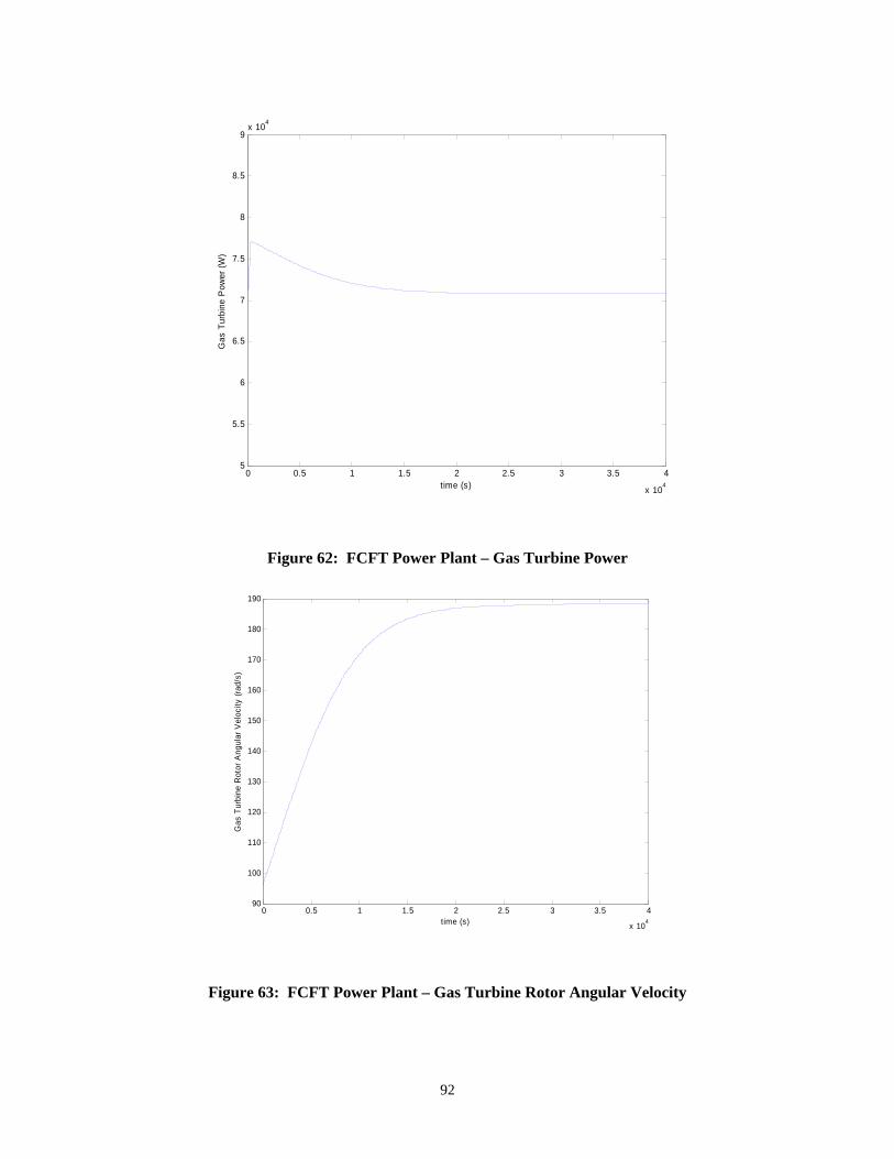
92
0 0.5 1 1.5 2 2.5 3 3.5 4
x 104
5
5.5
6
6.5
7
7.5
8
8.5
9x 10⁴
time (s)
Gas
Tur
bine
Pow
er (W
)
Figure 62: FCFT Power Plant – Gas Turbine Power
0 0.5 1 1.5 2 2.5 3 3.5 4
x 104
90
100
110
120
130
140
150
160
170
180
190
time (s)
Gas
Tur
bine
Rot
or A
ngul
ar V
eloc
ity (r
ad/s
)
Figure 63: FCFT Power Plant – Gas Turbine Rotor Angular Velocity

93
0 1000 2000 3000 4000 5000 6000 7000 8000 9000 100002
2.5
3
3.5
4
4.5
5
5.5
6
6.5x 10
5
time (s)
Tota
l Pow
er P
lant
Pow
er (W
)
Figure 64: FCFT Power Plant – Total Plant Power
4.2.3 FCGT – Integration Configuration Two
A second configuration for a combined fuel cell gas turbine system routes run the compressed
working fluid from the gas turbine directly through the cathode of the fuel cell. The output from
the cathode, as well as the leftover fuel from the anode is combusted and run through the turbine.
The exhaust gas of the turbine is then used to preheat the compressed air before it enters the
cathode of the fuel cell (Figure 65).

94
Compressor
Air In
Heat ExchangerGas Turbine Exhaust
Turbine Generator
Fuel Cell Power Out
Anode
+ -
Cathode
H2 In
combustorQ
Figure 65: Fuel Cell Gas Turbine Hybrid Power Plant Configuration Two
4.2.4 FCGT – Integration Configuration Two Simulation
Figure 66 shows the Simulink Model of the above configuration. The heat exchanger model is
excluded due to the fuel cell temperature assumed to be constant. Figures 67-70 show the results
of running this model. The fuel cell contributes 470 kW while the gas turbine contributes 430
kW. The gas turbine contributes much more power this time because excess fuel is combusted in
the working fluid before it expands through the turbine. The fluid exits the fuel cell at
approximately 1300K and is combusted to a temperature of 3000K. Therefore the fluid has a
much higher enthalpy than the previous configuration (Figure 59). The total power for the entire
power plant is 900 kW.

95
Figure 67 shows that the fuel cell power reaches steady state in approximately 7 s. This is faster
than the previous configuration due to the additional mass flow rate of the air being provided by
the compressor into the fuel cell. Figure 68 shows the power of the gas turbine stabilizing slower
than the fuel cell which is expected.

96
-138.8
T urbine T orque (Nm)1
Turbine Torque (Nm)
angular v elocity of rotor (rad/s)
mdot_in (kg/s)
torque to turn compressor (Nm)
Temperature out of combustor (K)
Turbine Torque Out (Nm)
Net Gas Tubine Power Out (W)
Output Temp (K)1
Turbine
9.035e+005
Total Power Out (W)1
Total Power Out (W)
Torque to turn Compressor (Nm)1
172.9
Torque to turn Compressor (Nm)
.5
Throttle Coef (gamma)
3169
Temperature Out of Combustor (K)1
Temperature Out of Combustor (K)
0
Stall Coeff (dim less)1
Stal l Coeff (dim less)
1.715e+005
Pressure Out of Compressor (Pa)1
Pressure Out of Compressor (Pa)
M icroscopic transport delayto aid in startup due to loop
.13
Mass Flow Rate of H2 (kg/s)
2.234
Mass Flow Rate (kg/s)1
Mass Flow Rate (kg/s)
4.322e+005
Gas T urbine Power (W)1
Gas Turbine Power (W)
Current (A)
m_dot H2 in (kg/s)
m_dot air in (kg/s)
Voltage
Power
Temp Out (K)
Air Out (kg/s)
H2 Out (kg/s)
Fuel Cel l
1571
FC Vol tage Out (V)1
FC Voltage Out (V)
4.713e+005
FC Power Out (W)1
FC Power Out (W)
Delayed Turbine T orque (Nm)
300
Current (A)
throttle coef (gamma)
turbine torque in (Nm)
mdot_compressor (kg/s)
pressure af ter comp (Pa)
angular v elocity (rad/s)
Stall Coef
Torque to turn Compressor (Nm)
Temp_out (K)
Compressor
mdot_f uel_in (kg/s)
mdot_oxid_in (kg/s)
Temp of Products Out (K)
mdot out of combusor (kg/s)
Combustor
96.138953237153
Angular Velocity of Rotor (rad/s)1Angular Veloci ty of Rotor (rad/s)
Figure 66: Fuel Cell Gas Turbine Hybrid Power Plant Simulink Model Configuration Two
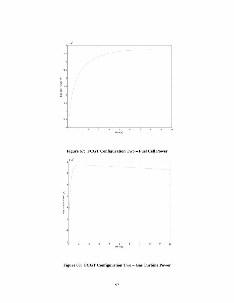
97
0 1 2 3 4 5 6 7 8 9 100
0.5
1
1.5
2
2.5
3
3.5
4
4.5
5x 10⁵
time (s)
Fuel
Cel
l Pow
er (W
)
Figure 67: FCGT Configuration Two – Fuel Cell Power
0 1 2 3 4 5 6 7 8 9 10-2
-1
0
1
2
3
4
5x 10⁵
time (s)
Gas
Tur
bine
Pow
er (W
)
Figure 68: FCGT Configuration Two – Gas Turbine Power

98
0 1 2 3 4 5 6 7 8 9 1095
95.2
95.4
95.6
95.8
96
96.2
96.4
96.6
96.8
97
time (s)
Gas
Tur
bine
Rot
or A
ngul
ar V
eloc
ity (r
ad/s
)
Figure 69: FCGT Configuration Two – Gas Turbine Rotor Angular Velocity
0 1 2 3 4 5 6 7 8 9 10-2.5
-2
-1.5
-1
-0.5
0
0.5
1x 10⁶
time(s)
Tota
l Pow
er (W
)
Figure 70: FCGT Configuration Two – Total Plant Power

99
5.0 PRELIMINARY CONTROLS
This section will discuss the control of the FCGT hybrid plant. The objective of the section is to
analyze the integrated system with respect to possible control methods. This entails identifying
effective control knobs based on the effect of step changes in different parameters. Once the
control knobs are identified, a simple proportional, integral, differential (PID) control mechanism
can be incorporated to determine if the non-linear system can be controlled. The main variable
to control is the turbine rotor speed. This controls the output power of the turbine and also the
air flow rate that flows through the fuel cell.
5.1 RESPONSE TO A STEP INPUT
Fuel cell – gas turbine hybrid configuration 2 will be analyzed dynamically due to its close
similarity to actual hybrid systems being built and studied today [8], [13]. A step input can be
attached to the inputs of the system to determine the system’s response. The inputs that can be
stepped are the throttle coefficient on the compressor model and the hydrogen input flow rate of
the fuel cell. Table 2 shows the parameters for the dynamic step response dynamic simulations.
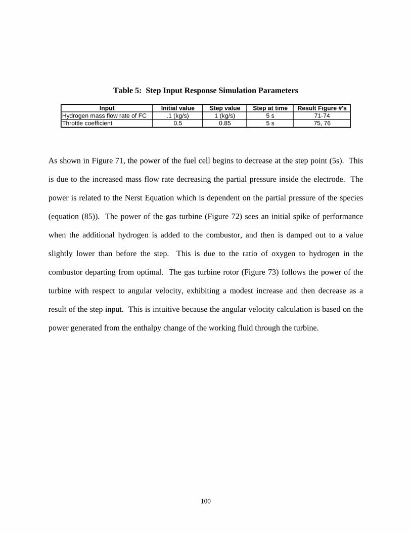
100
Table 5: Step Input Response Simulation Parameters
Input Initial value Step value Step at time Result Figure #'sHydrogen mass flow rate of FC .1 (kg/s) 1 (kg/s) 5 s 71-74Throttle coefficient 0.5 0.85 5 s 75, 76
As shown in Figure 71, the power of the fuel cell begins to decrease at the step point (5s). This
is due to the increased mass flow rate decreasing the partial pressure inside the electrode. The
power is related to the Nerst Equation which is dependent on the partial pressure of the species
(equation (85)). The power of the gas turbine (Figure 72) sees an initial spike of performance
when the additional hydrogen is added to the combustor, and then is damped out to a value
slightly lower than before the step. This is due to the ratio of oxygen to hydrogen in the
combustor departing from optimal. The gas turbine rotor (Figure 73) follows the power of the
turbine with respect to angular velocity, exhibiting a modest increase and then decrease as a
result of the step input. This is intuitive because the angular velocity calculation is based on the
power generated from the enthalpy change of the working fluid through the turbine.

101
0 1 2 3 4 5 6 7 8 9 10-2.5
-2
-1.5
-1
-0.5
0
0.5x 10
6
time (s)
Hyd
roge
n M
ass
Flow
Ste
p In
put F
uel C
ell P
ower
(W)
Figure 71: Fuel Cell Power during a Hydrogen Mass Flow Step Change
0 1 2 3 4 5 6 7 8 9 10-2
-1
0
1
2
3
4
5
6x 10⁵
time (s)
Hyd
roge
n M
ass
Flow
Ste
p In
put G
as T
urbi
ne P
ower
(W)
Figure 72: Gas Turbine Power during a Hydrogen Mass Flow Step Change

102
0 1 2 3 4 5 6 7 8 9 1096.11
96.12
96.13
96.14
96.15
96.16
96.17
96.18
Hyd
roge
n M
ass
Flow
Ste
p In
put R
otor
Ang
ular
Vel
ocity
(rad
/s)
Figure 73: Rotor Angular Velocity during a Hydrogen Mass Flow Step Change
0 1 2 3 4 5 6 7 8 9 10-2.5
-2
-1.5
-1
-0.5
0
0.5
1
1.5x 10⁶
time (s)
Hyd
roge
n M
ass
Flow
Ste
p In
put T
otal
Pla
nt P
ower
(W)
Figure 74: Total Plant Power during a Hydrogen Mass Flow Step Change

103
The throttle coefficient step input has almost no impact on the total power of the plant (Figure
75). This is because the throttle coefficient only slightly affects the pressure rise of the
compressor (Figure 76). This change is not enough to have an impact on the overall power of
the gas turbine and hence the plant. Therefore, the throttle coefficient can not be used to control
the system.
0 1 2 3 4 5 6 7 8 9 10-2.5
-2
-1.5
-1
-0.5
0
0.5
1x 10
6
time (s)
Thro
ttle
Coe
f. S
tep
Inpu
t - T
otal
Pla
nt P
ower
(W)
Figure 75: Total Plant Power during a Throttle Coefficient Step Input

104
0 1 2 3 4 5 6 7 8 9 101.35
1.4
1.45
1.5
1.55
1.6x 10⁵
time (s)
Thro
ttle
Coe
f. S
tep
Inpu
t - P
ress
ure
Out
put o
f Com
pres
sor (
Pa)
Figure 76: Pressure Output of Compressor during a Throttle Coefficient Step Input
5.2 TURBINE ROTOR SPEED CONTROL
The main control of the gas turbine would be the angular velocity of the rotor. The rotor velocity
is directly proportional to the power generated by the gas turbine portion of the power plant.
One way to control the angular velocity of the rotor is to introduce a temperature-controlled air
input into the working fluid stream before the fluid enters the turbine. The inlet temperature of
the working fluid is directly proportional to the power and torque developed by the turbine.
Therefore, the overall gas turbine power can be controlled using the temperature controlled air
input. This control could also be used to control the amount of fluid that runs through the fuel
cell because the rotor angular velocity is a factor in the amount of air drawn into the compressor.

105
Since the compressed air leaving the compressor flows directly through the fuel cell (FCGT
hybrid configuration 2), the air flow can also be controlled by the rotor velocity.
The temperature-controlled air input to the inlet stream of the turbine was incorporated into
integration configuration 2. A PID controller was added to the Simulink plant model to control
the temperature-controlled air inject signal. An angular velocity setpoint was added to have a
means for varying the target value. Various PID gains were tested to determine the optimal
settings for angular velocity control and are summarized in Table 3:
Table 6: Air Inject PID Control Settings
Setpoint 96 rad/sRun # P Gain I Gain D Gain Results Figure #
1 100000 100000 50000 772 100000 100000 35000 783 1000000 1000000 35000 794 1000000 1000000 500 80
Setpoint stepped 96 to 98 @ 1s, 98 to 94 @ 4s5 1000000 1000000 500 81, 82
As shown in Figure 77, the first run using the control scheme produced an unstable condition.
The angular velocity would oscillate about the setpoint before rising asymptotically to infinity.
This is due to the derivative gain being too high. It creates an “underdamped” system and the
output is not controlled.

106
0 1 2 3 4 5 6 7 8
x 10-3
0
50
100
150
200
250
time (s)
Rot
otr A
ngul
ar V
eloc
ity -
Uns
tabl
e (ra
d/s)
Figure 77: Angular Velocity with Control – PID gain settings 1 – Unstable
Figure 78 shows the results of the second run using different PID settings. The derivative gain
was reduced in an attempt to stabilize the system. The velocity does appear to remain near the
setpoint, but is still erratic with respect to the reference point (96 rad/s).

107
0 1 2 3 4 5 6 7 8 9 1096
96.5
97
97.5
98
98.5
99
time(s)
Rot
or A
ngul
ar V
eloc
ity S
tabl
e (ra
d/s)
Figure 78: Angular Velocity with Control – PID gain settings 2 – Semi-stable
For the third attempt, the derivative gain was kept constant and the proportional and integration
gains were increased by a factor of 10 to improve the steady state response. The output
stabilized macroscopically but the small oscillations remained due to the high derivative term.

108
0 0.2 0.4 0.6 0.8 1 1.2 1.4 1.6 1.8 296
96.5
97
97.5
98
98.5
time (s)
Rot
or A
ngul
ar V
eloc
ity (r
ad/s
)
Figure 79: Angular Velocity with Control – PID gain settings 3 – Stable with Oscillations
The forth PID setting uses a high decrease in the derivative gain to try and eliminate the micro-
oscillations in the output. Figure 80 shows that the signal is much less oscillatory. After a slight
overshoot on startup, and slight oscillations throughout, the output reaches the setpoint in
approximately 5 s.

109
0 1 2 3 4 5 6 7 8 9 1097.9
97.92
97.94
97.96
97.98
98
98.02
98.04
98.06
98.08
time (s)
Rot
or A
ngul
ar V
eloc
ity (r
ad/s
)
Figure 80: Angular Velocity with Control – PID gain settings 4 – Stable
To demonstrate that this type of controller can follow a stepped setpoint, a simulation was run
varying the setpoint at various times throughout the simulation (refer to Table 3). Figure 81
shows the setpoint signal and the output and shows that the output can follow small oscillations
in setpoint and the output power can be controlled.

110
0 1 2 3 4 5 6 7 893.5
94
94.5
95
95.5
96
96.5
97
97.5
98
98.5
time (s)
Rot
or A
ngul
ar V
eloc
ity (r
ad/s
)R
otor
Set
poin
t (ra
d/s)
Figure 81: Angular Velocity with Control – Stepped Setpoint – Stable
Figure 82 shows the response of the deviation of the fuel cell power due to a small change in
angular velocity of the gas turbine rotor. It is observed that the fuel cell power does vary slightly
with respect to rotor velocity. Therefore the angular velocity of the rotor could possibly be used
as a control for the output power of the fuel cell as well as the gas turbine.
Command signal – Rotor Angular Velocity Setpoint (green)
Response signal – Actual Rotor Velocity (blue)

111
500 550 600 650 700 750 800 850 900 950 10008.4
8.42
8.44
8.46
8.48
8.5
8.52
8.54
8.56
8.58
8.6x 10⁵
time (s)
Fuel
Cel
l Pow
er (W
)
Figure 82: Fuel Cell Power Reaction to Step in Rotor Angular Velocity

112
6.0 CONCLUSIONS AND FUTURE WORK
Models for the various components of a fuel cell gas turbine hybrid system have been modularly
developed using MATLAB and Simulink software. The component models are an axial flow
compressor, combustor, turbine, heat exchanger, and solid oxide fuel cell. Each component
model was developed and validated independently before incorporation into the complete
system. This modularity creates a flexible framework that can be used to create a virtually
limitless number of hybrid power plant combinations. Two hybrid configurations were
developed here. Both were simulated to observe general plant behavior such as power, rotor
velocity, and fuel cell voltage. One hybrid configuration was simulated with respect to dynamic
inputs. This consisted of stepping various inputs to determine the effect on the system outputs.
This can determine the control knobs that could possibly be used to control the plant. It was
found that varying the H2 input flow rate on the fuel cell had an impact on the total plant power
as well as the gas turbine power and rotor velocity. Therefore, this input could possibly be used
to control the output power of the plant. A separate control mechanism was implemented to
control the rotor velocity, and hence power, of the gas turbine. This consisted of injecting
temperature controlled air into the working fluid stream just before the turbine. This would
control the inlet temperature of the turbine as well as the enthalpy of the inlet fluid. Since the
power generated by the turbine is directly proportional to the change in enthalpy of the working
fluid, the output power, and the rotor velocity, of the gas turbine can be controlled. This scenario

113
was implemented on the hybrid model using a PID controller. It was found, after some tweaking
of the PID gains, that the angular velocity of the gas turbine could be controlled with respect to
an input set point using the air inject method. The controls analysis performed in this study is
not intended to be exhaustive, but rather to give a preliminary look at possible control methods
and directions. The main achievement of this study is the development of modular models that
can be used for future research. From a controls standpoint, additional studies could be
performed on linearization of the individual or combined models about a steady state operating
point. Standard controls analysis could then be used to characterize and design a control scheme.
Other control knobs could be analyzed and simulated as well.
The models developed here do not include some additional components that could be used to
better simulate a FCGT hybrid plant. For example, a fuel reformer could be incorporated into
the fuel cell model. This would more accurately represent an actual fuel cell cycle. Also, a
humidifier could be attached to the fuel cell. Valve dynamics could also be included to better
simulate the air inject and H2 input flow controls. In addition to the controls, these models could
be used for an efficiency study of various hybrid configurations. This could involve combining
multiple fuel cells and gas turbines with various heat exchangers. The study could also be
expanded to include the power delivery methods, such as synchronous vs. non-synchronous
turbines.

114
BIBLIOGRAPHY [1] F. K. Moore and E. M. Greitzer. A Theory of Post-Stall Transients in Axial Compression
Systems: Part 1 – Development of Equations. Transactions of the ASME, Volume 108, January 1986, p.68.
[2] E. M. Greitzer. Review – Axial Compressor Stall Phenomena. Transactions of the ASME, Volume 102, June 1980, p. 134.
[3] Jan Tommy Gravdahl and Olav Egeland. A Moore Greitzer Axial Compressor Model with Spool Dynamics. Proceedings of the 36th Conference on Decision and Control, San Diego, CA, USA, December 1997, p. 4714.
[4] Frank M. White. Fluid Mechanics. McGraw Hill, New York, NY, 1994.
[5] Christopher Fannin. Linear Modeling and Analysis of Thermoacoustic Instabilities in a Gas Turbine Combustor. PhD dissertation, Virginia Polytechnic Institute and State University, 2000.
[6] Michael Moran and Howard Shapiro. Fundamentals of Engineering Thermodynamics 3rd Ed. John Wiley and Sons, Inc., New York, NY, 1996.
[7] Frank Incropera and David DeWitt. Introduction to Heat Transfer. 3rd edition, John Wiley and Sons, Inc., New York, NY, 1985.
[8] James Larminie and Andrew Dicks. Fuel Cell Systems Explained. John Wiley and Sons, Inc., New York, NY, 2003.
[9] J. Padulles, G. W. Ault, J. R. McDonald. An Integrated SOFC Plant Dynamic Model for Power Systems Simulation. Journal of Power Sources, volume 86, 2000, p. 495.
[10] Shinji Kimijima and Nobuhide Kasagi. Performance Evaluation of Gas Turbine – Fuel Cell Hybrid Micro Generation System. Proceddings of ASME Turbo Expo, Amsterdam, The Netherlands, 2002.
[11] National Energy Technology Laborotory, Fuel Cell Handbook 6th edition. Morgantown, WV, 2002.

115
[12] Eric Liese, Randall Gemmen, Jose Rivera, Faryar, Jacob Brouwer. Development of Dynamic Modeling Tools For Solid Oxide and Molten Carbonate Hybrid Fuel Cell Gas Turbine Systems. Submitted for presentation at the International Gas Turbine Institiute meeting of the American Society of Mechanical Engineers, 2000.
[13] Eric Liese, Randall Gemmen, Faryar Jabbari, Jacob Brouwer. Technical Development Issues and Dynamic Modeling of a Gas Turbine and Fuel Cell Hybrid Systems.
[14] H. Cohen, G. F. C. Rogers, H. I. H. Saravanamuttoo. Gas Turbine Theory. John Wiley and Sons, Inc., New York, NY, 1973.
[15] The MathWorks. MATLAB and SIMULINK software. Natick, MA, 2002.
[16] Tuncer Cebeci and Peter Bradshaw. Physical and Computational Aspects of Convective Heat Transfer. Springer – Verlag, New York, NY.
[17] Trax Corporation. ProTrax Programmer’s Manual. Forest, VA.
[18] Pietro Bedont, Olivia Grillo, and Aristide Massardo. Off Design Performance Analysis of a Hybrid System Based on an Ecisting MCFC Stack. Proceedings of the ASME Turbo Expo, Amsterdam, the Netherlands, 2002.
[19] Maria-Teresa Basurto, Pericles Pilidis, and Richard Hales. Molten Carbonate Fuel Cell Gas Turbine Combined Cycle for Marine Propulsion. Part A: Design Point Operation. Proceedings of the ASME Turbo Expo, Amsterdam, the Netherlands, 2002.
[20] Eric Liese and Randall Gemmen. Dynamic Modeling Results of a 1 MW Molten Carbonate Fuel Cell/ Gas Turbine Power System. Proceedings of the ASME Turbo Expo, Amsterdam, The Netherlands, 2002.
[21] Francisco Jurado. Study of Molten Carbonate Fuel Cell – Microturbine Hybrid Power Systems. Journal of Power Sources, Volume 111, 2002.
[22] A. D. Rao and G. S. Samuelsen. A Thermodynamic Analysis of Tubular Solid Oxide Fuel Cell Based Hybrid Systems. Journal of Engineering for Gas Turbines and Power, Volume 125, 2003.
[23] A. F. Massardo and L. Magistri. Internal Reforming Solid Oxide Fuel Cell Gas Turbine Combined Cycles (IRSOFC-GT) – Part II: Exergy and Thermodynamic Analyses. Journal of Engineering for Gas Turbines and Power, Volume 125, 2003.