mixed logit estimation of willingness to pay … logit estimation of willingness to pay...

Mixed logit estimation of willingness to pay distributions: a comparison of

models in preference and WTP space using data from a health-related

choice experiment

Arne Risa Hole* Julie Riise Kolstad**

Abstract

Different approaches to modelling the distribution of WTP are compared using stated preference data

on Tanzanian Clinical Officers’ job choices and mixed logit models. The standard approach of

specifying the distributions of the coefficients and deriving WTP as the ratio of two coefficients

(estimation in preference space) is compared to specifying the distributions for WTP directly at the

estimation stage (estimation in WTP space). The models in preference space fit the data better than the

corresponding models in WTP space although the difference between the best fitting models in the

two estimation regimes is minimal. Moreover, the willingness to pay estimates derived from the

preference space models turn out to be unrealistically high for many of the job attributes. The results

suggest that sensitivity testing using a variety of model specifications, including estimation in WTP

space, is recommended when using mixed logit models to estimate willingness to pay distributions.

JEL: C5, I19, J4

Keywords: WTP space; Stated preference methods; Discrete choice; Mixed logit; Willingness

to pay

* Department of Economics, University of Sheffield. Email: [email protected]. ** Corresponding author. Department of Economics, University of Bergen. Email: [email protected].

1. Introduction

Health economists have a long tradition of estimating measures of willingness to pay (WTP)

for goods and services. Willingness to pay measures are considered useful for several reasons.

First, they can directly inform policy makers by providing information about how much

people value some goods or services and can thus inform the pricing of these goods or

services (Hanley et al., 2003). Second, WTP measures can be important inputs in economic

evaluations such as cost benefit analyses (Loomes, 2001; Oliver et al., 2002; Negrín et al.,

2008). Third, WTP measures can be a convenient tool to make relative comparisons and

rankings of the desirability of goods and services.

It is possible to estimate WTP measures in many ways; for instance the researcher can ask

respondents directly how much they are willing to pay for a certain service or good. However,

there are problems with methods like this. Direct questions about willingness to pay are

cognitively difficult to answer directly and respondents may have incentives to answer

strategically (Ryan, 2004; Hanley et al., 2003; Carson et al., 2001; Arrow et al., 1993).

Alternatively, WTP measures can be derived from discrete choice models estimated using

either revealed preference data or data from discrete choice experiments (DCEs). In these

cases, the WTP for an alternative attribute can be calculated as the ratio of the attribute

coefficient to the price coefficient (Train, 2003).

Mixed logit models are the state of the art tool applied in analysis of discrete choices and they

are increasingly applied in health economics (Hall et al., 2006; Lancsar et al., 2007; Regier et

al., 2009; Hole, 2008; King et al., 2007; Paterson et al., 2008; Negrín et al., 2008; Özdemir et

al., 2009). The mixed logit model makes it possible to account for heterogeneity in

preferences which are unrelated to observed characteristics and it has been shown that any

discrete choice random utility model can be approximated by an appropriately specified

mixed logit model (McFadden and Train, 2000). When estimating the mixed logit model the

researcher specifies that the distribution of preferences follow a particular distribution, for

instance a normal distribution. The parameters of this distribution, such as the mean and the

standard deviation in the case of a normal distribution, are then estimated using either

classical or Bayesian estimation techniques. Since the WTP for an attribute is given by the

ratio of the attribute coefficient to the price coefficient, the WTP from a mixed logit model is

given by the ratio of two randomly distributed terms. Depending on the choice of distributions

for the coefficients this can lead to WTP distributions which are heavily skewed and that may

not even have defined moments. A common approach to dealing with this potential problem is

to specify the price coefficient to be fixed. This is a convenient assumption as in this case the

distribution of the willingness to pay for an attribute is simply the distribution of the attribute

coefficient scaled by the fixed price coefficient. The problem is that it is often unreasonable to

assume that all individuals have the same preferences for price (Meijer and Rouwendal,

2006), so this approach implies an undesirable trade-off between reality and modelling

convenience. An alternative approach which allows the preferences for price to be

heterogeneous is to specify that the price coefficient is log-normally distributed. This ensures

that the WTP measures have defined moments since the price coefficient is constrained to be

positive, but the resulting WTP distribution can be highly skewed which may produce

unrealistic estimates of the means and standard deviations of WTP.

Train and Weeks (2005) suggest that a way to circumvent this problem is to estimate the

mixed logit model in WTP space rather than in preference space. This involves estimating the

distribution of willingness to pay directly by re-formulating the model in such a way that the

coefficients represent the WTP measures. The researcher then makes a priori assumptions

about the distributions of WTP rather than the attribute coefficients. This approach has been

found to produce more realistic WTP estimates in applications in other fields of economics

but to our knowledge the two methods have not been compared before in the health

economics literature.

In this study we focus on the implications of the choice of method to estimate WTP measures.

We compare the preference and WTP space approaches to modelling the distribution of

willingness to pay using stated preference data on Tanzanian Clinical Officers’ job choices.

We find that the results differ between the estimation regimes, suggesting that careful

sensitivity testing is necessary when using mixed logit models to estimate willingness to pay

distributions.

The paper is organised as follows. Section 2 provides a brief review of the use of mixed logit

models to estimate willingness to pay in the health economics literature. Literature from other

fields of economics where willingness to pay is estimated directly in WTP space is also

discussed. Sections 3 and 4 present the methodology and the data applied in the study. Section

5 presents the results and section 6 offers some concluding remarks.

2. Literature review

2.1 The use of mixed logit models to estimate willingness to pay in the health economics

literature

Although the mixed logit model is becoming increasingly popular in the field of health

economics there are still relatively few health-related studies that have used mixed logit

models to estimate willingness to pay measures. Among these studies the majority focus on

the mean or median on the WTP distribution while other aspects such as the skew and spread

of the distribution have received less attention. In the following we will present a brief review

of these studies with a particular focus on how their findings relate to estimating WTP.

Paterson et al. (2008) study smokers’ preferences for increased efficacy and other attributes of

smoking cessation therapies. Using a mixed logit model they estimate the willingness to pay

for different treatments among groups of smokers. They find evidence of substantial

preference heterogeneity and demonstrate that allowing for heterogeneity both improves the

fit of the model and enhances our understanding of the smokers’ preferences. The WTP for

the non-monetary attributes calculated at the median of the coefficient distributions is

reported.

Hole (2008) examines patients’ preferences for the attributes of a general practitioner

appointment using mixed and latent class logit models. Significant preference heterogeneity is

found for all attributes including cost and the mixed and latent class logit models fit the data

considerably better than the standard logit model. The WTP distributions are found to be

right-skewed as the mean WTP is substantially higher than the median WTP.

King et al. (2007) analyse patients’ preferences for managing asthma using mixed logit

models with random intercepts. They find that the mixed logit models fit the data better than a

standard logit and that a substantial amount of heterogeneity is unaccounted for by observable

characteristics. The modelling results are used to derive willingness to pay measures but in

this case the WTP estimates are fixed as only the constant terms are specified to be random.1

Negrín et al. (2008) apply mixed logit models to analyse the willingness to pay for alternative

policies for patients with Alzheimer’s disease. All coefficients are specified to be normally

distributed and both maximum simulated likelihood and hierarchical Bayes methods are used

to estimate the models. The authors find that there is significant heterogeneity in the

preferences for all the attributes including cost. The authors report WTP measures calculated

at the means of the coefficient distributions.

Regier et al. (2009) analyse preferences regarding genetic testing for developmental delay

using mixed logit models estimated using hierarchical Bayes and maximum simulated

likelihood. WTP measures are derived from the coefficients in the estimated models and it is

demonstrated that different distributional assumptions affect the WTP estimates. In particular

it is noted that when the cost parameter is assumed to be log normally distributed some WTP

estimates are found to be very high. The authors mention that estimation in WTP space may

be an alternative approach but do not pursue that option in their paper.

Finally, Özdemir et al (2009) analyse how “cheap talk” affects estimates of the willingness to

pay for health care using a mixed logit model estimated in WTP space. The WTP space

approach was chosen because it allows the authors to estimate WTP values directly and to

compare estimates from two different samples without adjusting for scale differences. The

authors conclude that being exposed to “cheap talk” has an impact on the estimated

willingness to pay.

2.2. Estimation of mixed logit models in WTP space

Train and Weeks (2005) show that WTP estimates can be estimated directly in a mixed logit

model by re-formulating the model in such a way that the estimated parameters represent the

parameters of the WTP distribution rather than the parameters of the usual coefficients. They

call this estimation in WTP space as opposed to the conventional approach which they call

estimation in preference space. The advantage of their approach is that the researcher

1 The authors state that this is due to the relatively low sample size in their application.

specifies the WTP distribution directly and therefore avoids the rather arbitrary choice of

WTP distribution that arises from dividing the coefficients of the non-monetary attributes by

the cost coefficient. This latter problem is neatly formulated by Scarpa et al. (2008):

“Models with conveniently tractable distributions for taste coefficients, such as the normal

and the log-normal, often obtain estimates that imply counter intuitive distributions of WTP.

This is due to the fact that the analytical expression for WTP involves a ratio where the

denominator is the cost coefficient.”

The WTP space method is not yet widely used, probably partly because it has not been

implemented in standard statistical software packages. It has been applied in a few studies,

however, in particular within the disciplines of environmental economics and marketing

(Train and Weeks, 2005; Sonnier et al., 2007; Scarpa et al., 2008; Balcombe et al., 2008;

Balcombe et al., 2009; Thiene and Scarpa, 2009). Train and Weeks (2005) and Sonnier et al.

(2007) use stated preference data on the choice of cars with different fuel systems and

cameras to compare the performance of models in WTP space to models in preference space.

Both studies use hierarchical Bayes to estimate the mixed logit models and their results are

similar in that they find that the models in preference space fit the data better than the models

estimated in WTP space. However, the models in WTP space were found to produce more

realistic WTP measures. Scarpa et al. (2008) use revealed preference data on destination

choices in the Alps to estimate models in preference and WTP space using both maximum

simulated likelihood and hierarchical Bayes. In their application the model in WTP space both

fits the data better and produces more realistic WTP estimates and the authors therefore

conclude that there is not necessarily a trade off between goodness of fit and reasonable WTP

estimates.

3. Methodology

The utility person n derives from choosing job j in choice situation t is specified as a function

of the wage, wnjt, and other non-monetary attributes of the job, xnjt:

njt n njt n njt njtU w xα β ε′= + + (1)

where αn and βn are individual-specific coefficients for the wage and the other attributes of the

job and εnjt is a random term. We assume that εnjt is extreme value distributed with variance

given by μn2(π2/6), where μn is an individual-specific scale parameter. Train and Weeks

(2005) show that dividing equation (1) by μn does not affect behaviour and results in a new

error term which is IID extreme value distributed with variance equal to π2/6:

njt n njt n njt njtU w c xλ ε′= + + (2)

where λn=αn/μn and cn=βn/μn.2 Train and Weeks (2005) call this specification the model in

preference space. By using the fact that WTP for the attributes is given by γn=cn/λn equation

(2) can be re-written as:

[ ]njt n njt n njt njtU w xλ γ ε′= + + (3)

which is what Train and Weeks (2005) call the model in WTP space. Models (2) and (3) are

of course behaviourally equivalent but the key thing to note is that standard assumptions

regarding the distributions of λn and cn in the preference space model, can lead to unusual

distributions for WTP. Assuming that λn and cn are normally distributed, for example, implies

that γn is a ratio of two normals which does not have defined moments. This is an unlikely

choice of distribution if we were to specify the distribution for the WTP directly as we do in

the WTP space model.

The coefficients in the preference space and WTP space models can be estimated by using

maximum simulated likelihood or Bayesian methods (Train, 2003). As in Thiene and Scarpa

(2009) we estimate the models using maximum simulated likelihood in the present paper.

4. Data

We use data from a discrete choice experiment on the choice of health service jobs among

Tanzanian final-year students training to be Clinical Officers (COs). The aim of the

experiment was to elicit the students’ preferences for different features of health service jobs 2 Strictly speaking we should introduce new notation for Unjt and εnjt to show that these are now equal to Unjt/μn and εnjt/μn but for the sake of readability we follow Train and Weeks (2005) here.

in order to advice Tanzanian policy makers on how rural jobs can be made more attractive to

Tanzanian health workers (Kolstad, 2008). Clinical Officers are health workers with the same

length of education as nurses, but with a more clinical orientation. They are in reality often

functioning as medical doctors, and this is in particular evident in the rural districts of

Tanzania. However, the job preferences among this important group of health workers have

not been given much attention earlier.

An extensive survey was administered to more than 300 final-year students. The discrete

choice experiment (DCE) formed the main part of the survey though demographics and other

background characteristics of the health workers such as gender, age and rural background

were also collected. Participation in the survey was voluntary and the participants were not

compensated in any way. 320 finalists (around 60% of all CO finalists in Tanzania in 2007)

from 10 randomly selected schools participated in the DCE. The CO training centres are

obliged to recruit students from all over Tanzania and there are no systematic differences

between students or teaching programs, hence the sample is likely to be representative of the

particular group of health workers that were studied. All finalists in the selected schools were

invited to participate and the data were mostly collected during school time, on the school

premises. This largely explains the response rate of around 96%, which is unusually high for a

DCE. After excluding incomplete responses and respondents from countries other than

Tanzania we were left with an estimation sample of 296 respondents.

The attributes in the choice experiment were chosen following extensive literature searches

and early in-depth interviews to identify the most important aspects of health service jobs. We

used a D-optimal design based on the covariance matrix of a multinomial logit model with all

the coefficients set equal to zero to construct the hypothetical choice situations. The result was

a set of 32 choice situations that were randomly divided into two blocks. Each respondent was

presented with 16 choice situations where each of these represented the choice between two

hypothetical jobs. The jobs consisted of seven attributes which included the wage of the job,

education prospects and other characteristics related to the location of the job and the facilities

of the workplace. A list of the attributes and their levels is reported in Appendix 1 and an

example choice situation can be found in Appendix 2. The attributes and the design of the

DCE are described in more detail in (Kolstad, 2008).

5. Results

5.1 Models in preference space

Table 1 shows the results for the models in preference space.3 Model 1 is a simple logit model

and model 2 is a mixed logit model with independent random coefficients for all the attributes

except wage. These two models were included as benchmark specifications as they are both

common in the DCE literature. Model 3 is equivalent to Model 2 except that it allows for

preference heterogeneity in terms of wages and Model 4 also allows for non-zero correlations

between the wage coefficient and the other coefficients and between the education

coefficients. Given the high number of random coefficients in the model we decided that a

model with a completely unrestricted correlation matrix would be too demanding to estimate

and we therefore allow for non-zero correlations between the coefficients that to us seemed

more likely to be correlated a priori4. In all the mixed logit models, the coefficients for wage,

education, infrastructure and equipment are given a log-normal distribution5, while the rest of

the coefficients are normally distributed. We use 1000 Halton draws in the estimation of the

mixed logit models with independent coefficients and 2500 Halton draws to estimate the

model with correlated coefficients.6

[Table 1 around here]

In general the coefficients in the models in Table 1 have the expected signs and the estimates

are fairly consistent across models in terms of signs and significance. All else equal the

respondents prefer a job with higher wages and they prefer to have the possibility of further

education after 2, 4 and 6 years to no further education. They prefer a job where sufficient

equipment is provided to one without sufficient equipment and a job which offers decent

housing and infrastructure to one that does not. In terms of location the respondents prefer to

work in a district headquarter to working in a regional headquarter or in a location which is a

3 The mixed logit models in preference space are estimated in Stata using the mixlogit command (Hole, 2007). The models in WTP space are estimated using a modified version of this command. All models were estimated using alternative starting values to reduce the likelihood of the algorithm getting trapped in a local optimum. 4 The selection of correlations was informed by evidence from interviews with a subset of the respondents. 5 We report the parameters of the log-normal distribution rather than the underlying normal distribution, although the latter parameterisation was used at the estimation stage. The standard errors of the parameters are calculated using the delta method. 6 We increased the number of draws in the estimation of the more complex model as this was needed to produce stable results.

3-hour (or longer) bus ride from the district headquarters. The least popular location is the

capital, Dar es Salaam. This may seem surprising but there are several plausible explanations

for this finding. Living costs are very high in Dar es Salaam compared even to other cities in

Tanzania, but perhaps more importantly the likelihood of being in charge of a health facility

and to be able to practice as a clinician is smaller in Dar es Salaam, where most of the “real”

doctors are based. The coefficients for the workload attribute and for being located in a

regional headquarter are insignificant in all the models.7 The constant term is also found to be

consistently insignificant, which is expected since a significant constant term would indicate a

preference for job “A” over job “B” (or vice versa) net of the influence of the alternative

attributes. Since no information is provided about the jobs apart from the attributes the

constant term should theoretically equal zero. The constant is nevertheless often included in

the model as a test for specification error (Scott, 2001) and we follow that convention here.

The results in Table 1 show that there is a substantial amount of heterogeneity in the

preferences for the various job attributes. In all the mixed logit models there is evidence of

significant heterogeneity in the preferences for equipment, infrastructure, workload and

education after 2 years of service. In addition Models 3 and 4 show significant heterogeneity

in the preferences for working in Dar es Salaam and, importantly, in the preferences for the

wage attribute. The latter finding implies that model 2 where the wage parameter is assumed

to be fixed is too restrictive.


The correlations between the estimated coefficients in model 4 are reported in Table 2. It can

be seen from the table the coefficients are in general quite highly correlated, in particular the

education coefficients. This finding seems plausible as a person that value education after 4

years highly is also likely to value education after 2 years highly. The wage coefficient is also

found to be highly correlated with the coefficients for education. For policy purposes, it is

important to be aware of the possible implications of this finding; strong preferences for

education do not necessarily reflect a genuine preference for knowledge and skills, but may

indirectly capture preferences for higher salaries which are strongly related to higher

education in Tanzania. The wage coefficient is also found to be positively correlated with the

7 See the discussion in Kolstad (2008) for some possible explanations of this finding.

coefficient for improved infrastructure, while the coefficient for sufficient equipment is

negatively correlated with the wage coefficient. This indicates that those who put a high

weight on working at a facility with sufficient equipment and drugs are less concerned with

high wages, suggesting that at least some of the COs are motivated by other factors than mere

economic incentives.

We find that the goodness of fit increases with the flexibility of the model. Model 4, which

allows the coefficients to be correlated, fits the data better than Model 3 in which they are

assumed to be independent. Models 3 and 4 both have considerably better fit than Model 2,

which is another indication of the significant preference heterogeneity in terms of wages in

the data. As expected the worst performing model is the standard logit which does not allow

for any preference heterogeneity. This result is confirmed by all the applied information

criteria: the log likelihood and the Akaike (AIC) and Swartz (BIC) criteria.

5.2 Willingness to pay in preference space

Table 3 shows the mean, median and standard deviation of the willingness to pay measures

derived from Models 1-4.8 The mean willingness to pay for education opportunities, decent

infrastructure and a health facility with sufficient equipment is generally high. The

respondents are willing to sacrifice the largest amount of their salary to have the opportunity

to continue their education after 2 years of service. The ranking of these attributes varies

somewhat between the models with independent coefficients (Models 1-3) and the model with

correlated coefficients (Model 4). The main difference is that in the latter model education

after 4 years is ranked higher than in the other models.


The means of the WTP measures derived from Models 1 and 2 are quite similar and

substantially lower than those from Models 3 and 4 in which the wage coefficient is specified

to be random. The mean willingness to pay for decent infrastructure, for instance, increases

from 237.03 TSH per month in Model 2 to 465.913 TSH per month in Model 3. When

8 These figures are calculated by using simulation. The simulated WTP distributions are obtained by dividing draws from the distributions of the non-monetary coefficients by draws from the distributions of the wage coefficient. 10,000 draws were used in the calculations.

bearing in mind that the starting salary for a public CO is just above 200.000 TSH per month

the WTP values from Model 3 and 4 seem very high. The question is whether this increase in

the mean WTP reflects the models’ ability to capture preference heterogeneity in terms of

wages or whether it is an artefact of the particular distribution we have chosen for WTP. It

can be seen that the WTP distributions are highly skewed as the absolute value of the median

is consistently much lower than the mean. The introduction of correlation between the

coefficients decreases the means of the WTP measures somewhat, but their distributions are

still highly skewed. The standard deviations of the WTP measures are also very large in

models 3 and 4. Again this may simply reflect a high degree of preference heterogeneity but it

may also be a result of our choice of distributions for the coefficients and hence WTP.

[Tables 4a and 4b around here]

The correlations between the WTP measures derived from Models 3 and 4 are shown in

Tables 4a and 4b. It can be seen from the tables that there is a high degree of correlation

between the WTP measures. In particular, the WTP for provision of decent housing is

positively correlated with WTP for education and for working in a district headquarter. The

WTP for the different education levels are highly correlated with each other. The WTP for

sufficient equipment is more highly correlated with the other WTP measures in model 4 than

in model 3 while the other WTP measures are more highly correlated in model 3.

5.3 Models in WTP space

Table 5 presents the estimates from the models in WTP space. Models 5 and 6 in this table are

analogous to models 3 and 4 in preference space in that all the attribute coefficients are

assumed to be random but the coefficients in model 5 are independent while some of the

coefficients in model 6 are allowed to be correlated. In particular, the non-monetary attributes

are specified to be correlated with the wage coefficient and the coefficients for education after

2, 4 and 6 years are specified to be correlated with each other. As in the preference space

models the coefficients for wage, education, infrastructure and equipment are given log-

normal distributions, while the rest of the coefficients are normally distributed. In this case,

however, the chosen distributions for the non-monetary attributes represent the distributions

of WTP for these attributes. Both models are estimated using 2500 Halton draws.

It is evident from the table that the means of the WTP measures are much lower than those

derived from the corresponding models from preference space. This is in line with the

findings in Sonnier et al. (2007), Train and Weeks (2005) and Scarpa et al. (2008). It is also

interesting to note that the means of the WTP measures in Models 5 and 6 are similar to those

derived from the simplest models in preference space (Models 1 and 2).


The standard deviations of the WTP measures are generally high, indicating that there is a

substantial amount of heterogeneity in the respondents’ preferences, although the standard

deviations are substantially smaller than in preference space. Similarly, the WTP distributions

for the log-normally attributes are skewed as the means are much larger than the medians, but

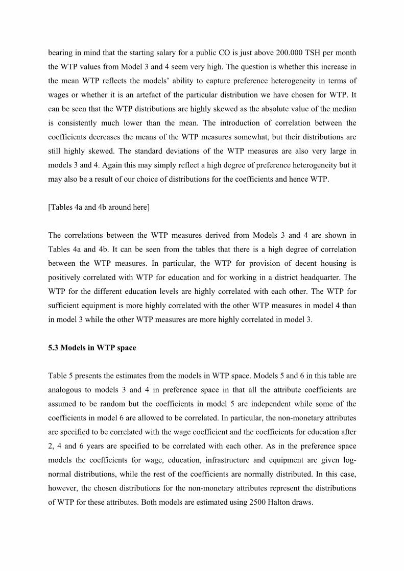
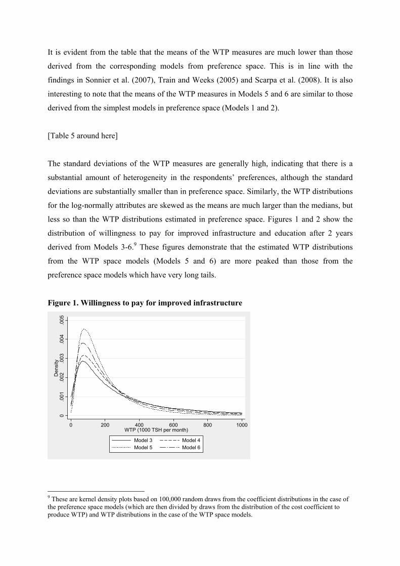
less so than the WTP distributions estimated in preference space. Figures 1 and 2 show the

distribution of willingness to pay for improved infrastructure and education after 2 years

derived from Models 3-6.9 These figures demonstrate that the estimated WTP distributions

from the WTP space models (Models 5 and 6) are more peaked than those from the

preference space models which have very long tails.

Figure 1. Willingness to pay for improved infrastructure

0.0

01.0

02.0

03.0

04.0

05D

ensi

ty

0 200 400 600 800 1000WTP (1000 TSH per month)

Model 3 Model 4Model 5 Model 6

9 These are kernel density plots based on 100,000 random draws from the coefficient distributions in the case of the preference space models (which are then divided by draws from the distribution of the cost coefficient to produce WTP) and WTP distributions in the case of the WTP space models.

Figure 2. Willingness to pay for education after 2 years 0

.000

5.0

01.0

015

.002

.002

5D

ensi

ty

0 500 1000 1500WTP (1000 TSH per month)

Model 3 Model 4Model 5 Model 6

It should also be noted that there evidence of significant heterogeneity in the WTP for housing

and for education after 6 years of service in WTP space but not in preference space. This

observation demonstrates the possibility of obtaining different qualitative results depending

on the estimation regime. We also find some evidence of this when analysing the implied

ranking of the means of the WTP distributions for the different attributes. The ranking differs

between the preference space and WTP space models, although education after 2 years of

service is the most highly ranked attribute according to all the models.


Table 6 shows the correlations between the WTP measures and the wage coefficient and the

WTP for education derived from Model 6. It can be seen that the WTP for sufficient

equipment is negatively correlated with the wage coefficient. This suggests that respondents

who find the facilities of the workplace especially important are less concerned with higher

wages which confirms our result in preference space. The consistent pattern of highly

correlated willingness to pay for education is not found in WTP space, however. The WTP

measures for education after 2 and 4 years are highly correlated, but education after 6 years is

found to be negatively correlated with education after 2 and 4 years. This observation may be

an indication that COs see education after 6 years as something qualitatively different from

education after a shorter time of service.

By comparing Tables 1 and 5 it can be seen that the fit of the models in WTP space is not as

good as that of the corresponding models in preference space. This is in line with Train and

Weeks (2005) and Sonnier et al. (2007), while Scarpa et al. (2008) find that the WTP space

model fits their data better. The result in the present application is not as clear-cut as it may

seem at first glance, however. For all practical purposes the difference in goodness of fit

between Model 4 and Model 6 is negligible according to all the applied information criteria.

Regardless of the estimation regime there is a more substantial difference in fit between the

models which allow the coefficients to be correlated (Models 4 and 6) and the models in

which the coefficients are assumed to be independent (Models 3 and 5). It is also worth noting

that both the models estimated in WTP space fit the data better than the preference space

model with a fixed wage coefficient. These results imply that allowing for non-zero

correlations between the coefficients and for heterogeneity in the preferences for the wage

attribute affect the fit of the model more than whether the model is estimated in preference or

WTP space.

6. Concluding remarks

Due to practical considerations it is common to specify the coefficient for the monetary

attribute in choice models to be fixed. This specification represents a trade-off between

realism and modelling convenience as it is often unrealistic to assume that all respondents

have the same preferences regarding the price of a good or the wage of a job. Relaxing the

assumption of preference homogeneity is not straightforward, however, as it may lead to

implausible distributions for willingness to pay. In this paper we compare models estimated in

preference and WTP space and find that the estimated willingness to pay distributions differ

markedly in the two estimation regimes. When the preferences for wage are allowed to be

heterogeneous the means of the WTP distributions estimated in preference space turn out to

be unrealistically high for many of the attributes while those estimated directly in WTP space

are more realistic.

The models in preference space fit the data in our study better than the corresponding models

in WTP space, but this distinction is not clear-cut as the best fitting models in the two

estimation regimes have very similar goodness of fit. Allowing for heterogeneity in the

preferences for wages and allowing for non-zero correlations between the coefficients is

found to affect the goodness of fit of the models more than whether the model is estimated in

preference or WTP space.

Our results suggest that sensitivity testing using a variety of model specifications, including

estimation in WTP space, is recommended when using mixed logit models to estimate

willingness to pay distributions.

References

Arrow, K., Solow, R., Portney, P., Leamer, E., Radner, R. and Schumann, H. (1993). Report

of the NOAA panel of contingent valuation Federal Register 10, 4601-14.

Balcombe, K., Bailey, A., Chalak, A. and Fraser, I. (2008). Modifying willingness to pay

estimates where respondents mis-report their preferences. Applied Economics Letters

15, 327 - 330.

Balcombe, K., Chalak, A. and Fraser, I. (2009). Model selection for the mixed logit with

Bayesian estimation. Journal of Environmental Economics and Management 57, 226-

237.

Carson, R. T., Flores, N. E. and Meade, N. S. (2001). Contingent valuation: controversies and

evidence. Environmental and Resource Economics 19, 173-210.

Hall, J., Fiebig, D. G., King, M. T., Hossain, I. and Louviere, J. (2006). What influences

participation in genetic carrier testing? Results from a discrete choice experiment.

Journal of Health Economics 25, 520-537.

Hanley, N., Ryan, M. and Wright, R. (2003). Estimating the monetary value of health care:

Lessons from environmental economics. Health Economics 12, 3-16.

Hole, A. R. (2007). Fitting mixed logit models by using maximum simulated likelihood. The

Stata Journal 7, 388-401.

Hole, A. R. (2008). Modelling heterogeneity in patients' preferences for the attributes of a

general practitioner appointment. Journal of Health Economics 27, 1078-1094.

King, M. T., Hall, J., Lancsar, E., Fiebig, D., Hossain, I., Louviere, J., Reddel, H. and Jenkins,

C. R. (2007). Patient preferences for managing asthma: results from a discrete choice

experiment. Health Economics 16, 703-717.

Kolstad, J. R. (2008). How to make rural jobs more attractive to health workers. Findings

from a discrete choice experiment in Tanzania. In Working paper 15/2008,

Department of economics, University of Bergen.(Ed, Department of Economics, U. o.

B.). Working paper 15/2008, Department of Economics, University of Bergen.

Lancsar, E., Hall, J., King, M., Kenny, P. and Louviere, J. (2007). Patient preferences for

managing asthma: Results from a discrete choice experiment. Respirology 12, 127-

136.

Loomes, G. (2001). The use of cost-effectiveness thresholds outside the health sector. In Cost-

effectiveness Thresholds: Economic and Ethical Issues(Eds, Towse, A., Pritchard, C.

and Devlin, N.). London: Office of Health Economics.

McFadden, D. and Train, K. (2000). Mixed MNL for discrete response. Journal of Applied

Econometrics 15, 447-470.

Meijer, E. and Rouwendal, J. (2006). Measuring Welfare Effects in Models with Random

Coefficients. Journal of Applied Econometrics 21, 227-244.

Negrín, M. A., Pinilla, J. and León, C. J. (2008). Willingness to pay for alternative policies for

patients with Alzheimer's Disease. Health Economics, Policy and Law 3, 257-275.

Oliver, A., Healey, A. and Donaldson, C. (2002). Choosing the method to match the

perspective: economic assessment and its implications for health-services efficiency

Lancet 359, 1771-1774.

Paterson, R. W., Boyle, K. J., Parmeter, C. F., Neumann, J. E. and Civita, P. d. (2008).

Heterogeneity in preferences for smoking cessation. Health Economics 17, 1363-1377.

Regier, D. A., Ryan, M., Phimister, E. and Marra, C. A. (2009). Bayesian and classical

estimation of mixed logit: An application to genetic testing. Journal of Health

Economics 28, 598-610.

Ryan, M. (2004). A comparison of stated preference methods for estimating monetary values.

Health Economics 13, 291-296.

Scarpa, R., Thiene, M. and Train, K. (2008). Utility in willingness to pay space: A tool to

address confounding random scale effects in destination choice to the Alps. American

Journal of Agricultural Economics 90, 94-1010.

Scott, A. (2001). Eliciting GPs' preferences for pecuniary and non-pecuniary job

characteristics. Journal of Health Economics 20, 329-347.

Sonnier, G., Ainslie, A. and Otter, T. (2007). Heterogeneity distributions of willingness-to-

pay in choice models. Quantitative Marketing Economics 5, 313-331.

Thiene, M. and Scarpa, R. (2009). Deriving and Testing Efficient Estimates of WTP

Distributions in Destination Choice Models Environment and Resource Economics In

press.

Train, K. E. (2003). Discrete Choice Methods with Simulation. Cambridge University Press.

Train, K. E. and Weeks, M. (2005). Discrete choice models in preference space and

willingness-to-pay space. In Application of simulation methods in environmental and

resource economics(Eds, Scarpa, R. and Alberini, A.). Dordrecht: Springer, 1-16.

Özdemir, S., Johnson, F. R. and Hauber, A. B. (2009). Hypothetical bias, cheap talk, and

stated willingness to pay for health care. Journal of Health Economics In press.

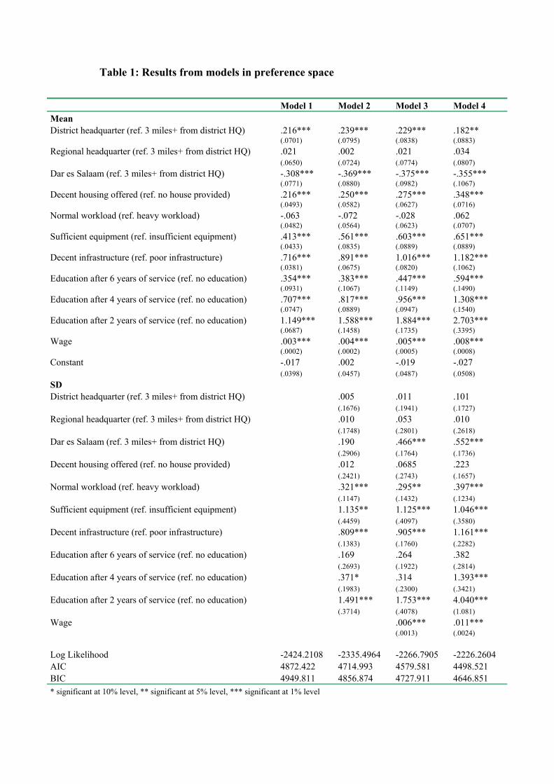
Table 1: Results from models in preference space

Model 1 Model 2 Model 3 Model 4 Mean District headquarter (ref. 3 miles+ from district HQ) .216*** .239*** .229*** .182** (.0701) (.0795) (.0838) (.0883) Regional headquarter (ref. 3 miles+ from district HQ) .021 .002 .021 .034 (.0650) (.0724) (.0774) (.0807) Dar es Salaam (ref. 3 miles+ from district HQ) -.308*** -.369*** -.375*** -.355*** (.0771) (.0880) (.0982) (.1067) Decent housing offered (ref. no house provided) .216*** .250*** .275*** .348*** (.0493) (.0582) (.0627) (.0716) Normal workload (ref. heavy workload) -.063 -.072 -.028 .062 (.0482) (.0564) (.0623) (.0707) Sufficient equipment (ref. insufficient equipment) .413*** .561*** .603*** .651*** (.0433) (.0835) (.0889) (.0889) Decent infrastructure (ref. poor infrastructure) .716*** .891*** 1.016*** 1.182*** (.0381) (.0675) (.0820) (.1062) Education after 6 years of service (ref. no education) .354*** .383*** .447*** .594*** (.0931) (.1067) (.1149) (.1490) Education after 4 years of service (ref. no education) .707*** .817*** .956*** 1.308*** (.0747) (.0889) (.0947) (.1540) Education after 2 years of service (ref. no education) 1.149*** 1.588*** 1.884*** 2.703*** (.0687) (.1458) (.1735) (.3395) Wage .003*** .004*** .005*** .008*** (.0002) (.0002) (.0005) (.0008) Constant -.017 .002 -.019 -.027 (.0398) (.0457) (.0487) (.0508) SD District headquarter (ref. 3 miles+ from district HQ) .005 .011 .101 (.1676) (.1941) (.1727) Regional headquarter (ref. 3 miles+ from district HQ) .010 .053 .010 (.1748) (.2801) (.2618) Dar es Salaam (ref. 3 miles+ from district HQ) .190 .466*** .552*** (.2906) (.1764) (.1736) Decent housing offered (ref. no house provided) .012 .0685 .223 (.2421) (.2743) (.1657) Normal workload (ref. heavy workload) .321*** .295** .397*** (.1147) (.1432) (.1234) Sufficient equipment (ref. insufficient equipment) 1.135** 1.125*** 1.046*** (.4459) (.4097) (.3580) Decent infrastructure (ref. poor infrastructure) .809*** .905*** 1.161*** (.1383) (.1760) (.2282) Education after 6 years of service (ref. no education) .169 .264 .382 (.2693) (.1922) (.2814) Education after 4 years of service (ref. no education) .371* .314 1.393*** (.1983) (.2300) (.3421) Education after 2 years of service (ref. no education) 1.491*** 1.753*** 4.040*** (.3714) (.4078) (1.081) Wage .006*** .011*** (.0013) (.0024) Log Likelihood -2424.2108 -2335.4964 -2266.7905 -2226.2604 AIC 4872.422 4714.993 4579.581 4498.521 BIC 4949.811 4856.874 4727.911 4646.851 * significant at 10% level, ** significant at 5% level, *** significant at 1% level

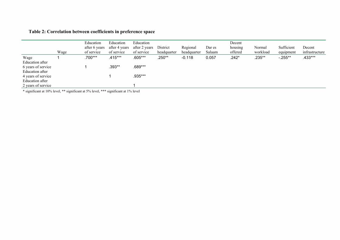
Table 2: Correlation between coefficients in preference space

Wage

Education after 6 years of service



District headquarter

Regional headquarter

Dar es Salaam

Decent housing offered

Normal workload

Sufficient equipment

Decent infrastructure

Wage 1 .700*** .415*** .605*** .250** -0.118 0.057 .242* .235** -.255** .433*** Education after 6 years of service 1 .393** .689*** Education after 4 years of service 1 .935*** Education after 2 years of service 1 * significant at 10% level, ** significant at 5% level, *** significant at 1% level

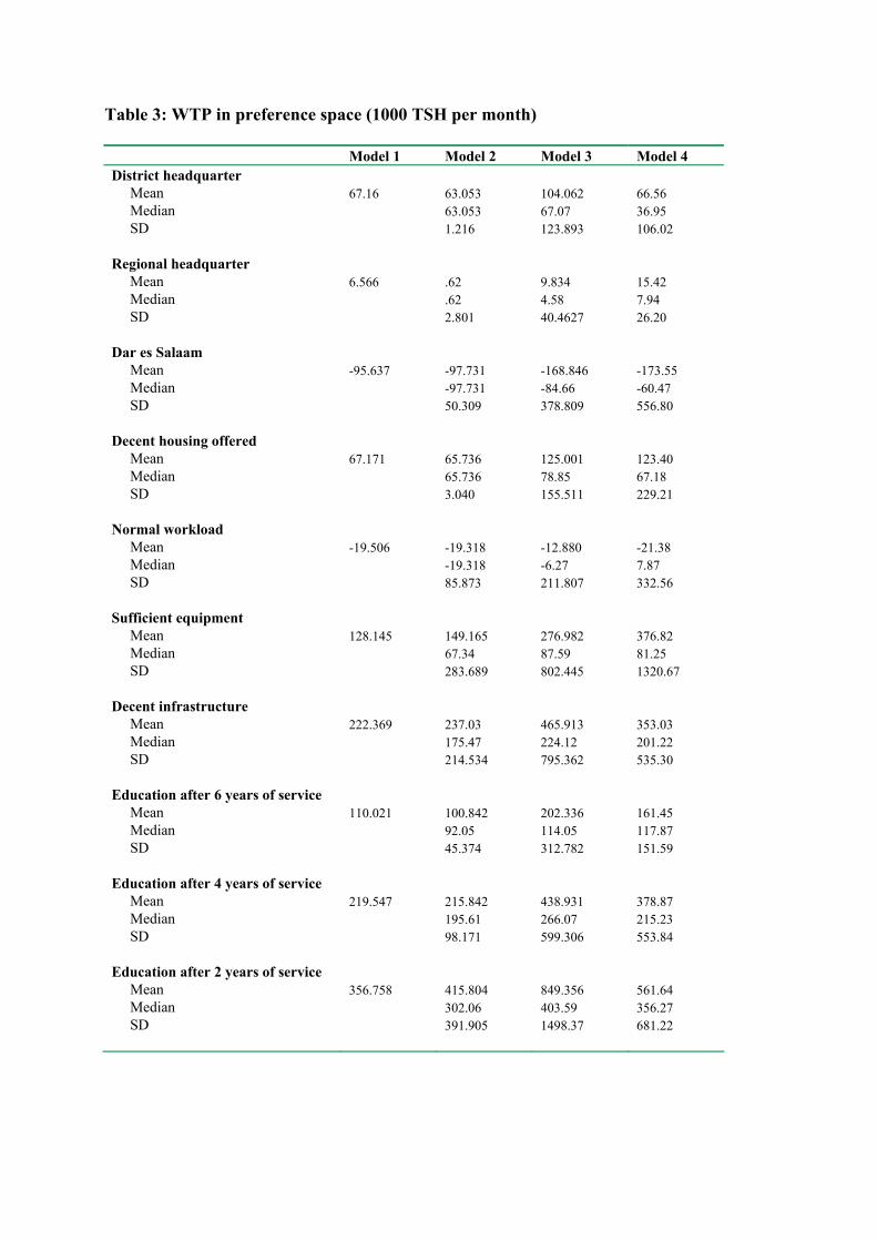
Table 3: WTP in preference space (1000 TSH per month) Model 1 Model 2 Model 3 Model 4 District headquarter Mean 67.16 63.053 104.062 66.56 Median 63.053 67.07 36.95 SD 1.216 123.893 106.02 Regional headquarter Mean 6.566 .62 9.834 15.42 Median .62 4.58 7.94 SD 2.801 40.4627 26.20 Dar es Salaam Mean -95.637 -97.731 -168.846 -173.55 Median -97.731 -84.66 -60.47 SD 50.309 378.809 556.80 Decent housing offered Mean 67.171 65.736 125.001 123.40 Median 65.736 78.85 67.18 SD 3.040 155.511 229.21 Normal workload Mean -19.506 -19.318 -12.880 -21.38 Median -19.318 -6.27 7.87 SD 85.873 211.807 332.56 Sufficient equipment Mean 128.145 149.165 276.982 376.82 Median 67.34 87.59 81.25 SD 283.689 802.445 1320.67 Decent infrastructure Mean 222.369 237.03 465.913 353.03 Median 175.47 224.12 201.22 SD 214.534 795.362 535.30 Education after 6 years of service Mean 110.021 100.842 202.336 161.45 Median 92.05 114.05 117.87 SD 45.374 312.782 151.59 Education after 4 years of service Mean 219.547 215.842 438.931 378.87 Median 195.61 266.07 215.23 SD 98.171 599.306 553.84 Education after 2 years of service Mean 356.758 415.804 849.356 561.64 Median 302.06 403.59 356.27 SD 391.905 1498.37 681.22

Table 4a: Correlation between WTP derived from models in preference space with uncorrelated coefficients.






Dar es Salaam


Normal workload



Education after 6 years of service 1 Education after 4 years of service .7073 1 Education after 2 years of service .5261 .6109 1 District headquarter .7700 .9187 .6534 1 Regional headquarter .1774 .2498 .2239 .2766 1 Dar es Salaam -.4208 -.4883 -.3373 -.5348 -.1477 1 Decent housing offered .7103 .8733 .6136 .9444 .2925 -.5034 1 Normal workload .0305 -.0092 .0326 -.0167 -.0404 .0288 -.0383 1 Sufficient equipment .3441 .3745 .2840 .4150 .0561 -.2345 .3667 .0461 1 Decent infrastructure .5850 .6394 .4626 .6876 .1941 -.3824 .6301 -.0471 .3116 1 Table 4b: Correlation between WTP derived from models in preference space with correlated coefficients






Dar es Salaam


Normal workload



Education after 6 years of service 1 Education after 4 years of service .5252 1 Education after 2 years of service .5080 .8895 1 District headquarter .4771 .3559 .1689 1 Regional headquarter .7226 .5106 .3145 .6853 1 Dar es Salaam -.4215 -.2764 -.1649 -.4488 -.5939 1 Decent housing offered .3429 .2852 .1494 .2518 .3579 -.1617 1 Normal workload -.3753 -.2721 -.2116 -.3501 -.3934 .2097 -.1109 1 Sufficient equipment .4952 .3927 .2793 .5339 .5488 -.3707 .3011 -.2259 1 Decent infrastructure .3041 .2220 .0403 .4282 .6154 -.424 .1263 -.3311 .3663 1

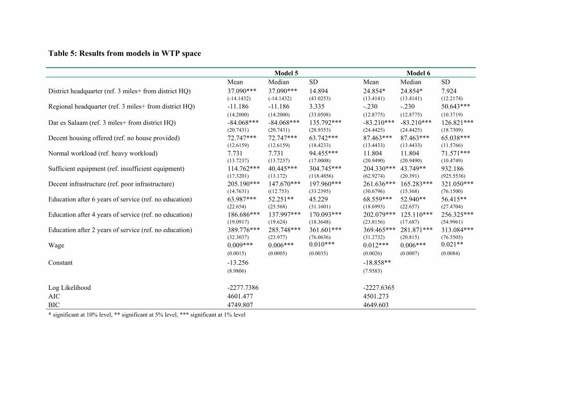
Table 5: Results from models in WTP space

Model 5 Model 6 Mean Median SD Mean Median SD District headquarter (ref. 3 miles+ from district HQ) 37.090*** 37.090*** 14.894 24.854* 24.854* 7.924 (-14.1432) (-14.1432) (43.0253) (13.4141) (13.4141) (12.2174) Regional headquarter (ref. 3 miles+ from district HQ) -11.186 -11.186 3.335 -.230 -.230 50.643*** (14.2000) (14.2000) (33.0508) (12.8775) (12.8775) (10.3719) Dar es Salaam (ref. 3 miles+ from district HQ) -84.068*** -84.068*** 135.792*** -83.210*** -83.210*** 126.821*** (20.7431) (20.7431) (28.9353) (24.4425) (24.4425) (18.7309) Decent housing offered (ref. no house provided) 72.747*** 72.747*** 63.742*** 87.463*** 87.463*** 65.038*** (12.6159) (12.6159) (18.4233) (13.4433) (13.4433) (11.5766) Normal workload (ref. heavy workload) 7.731 7.731 94.455*** 11.804 11.804 71.571*** (13.7237) (13.7237) (17.0008) (20.9490) (20.9490) (10.4749) Sufficient equipment (ref. insufficient equipment) 114.762*** 40.445*** 304.745*** 204.330*** 43.749** 932.186 (17.3201) (13.172) (118.4856) (62.9274) (20.391) (925.5536) Decent infrastructure (ref. poor infrastructure) 205.190*** 147.670*** 197.960*** 261.636*** 165.283*** 321.050*** (14.7631) ((12.753) (33.2395) (30.6796) (15.368) (76.1500) Education after 6 years of service (ref. no education) 63.987*** 52.251** 45.229 68.559*** 52.940** 56.415** (22.654) (25.568) (31.1601) (18.6993) (22.657) (27.4704) Education after 4 years of service (ref. no education) 186.686*** 137.997*** 170.093*** 202.079*** 125.110*** 256.325*** (19.0917) (19.624) (18.3648) (23.8156) (17.687) (54.9961) Education after 2 years of service (ref. no education) 389.776*** 285.748*** 361.601*** 369.465*** 281.871*** 313.084*** (32.3037) (23.977) (76.0636) (31.2732) (20.815) (76.5505) Wage 0.009*** 0.006*** 0.010*** 0.012*** 0.006*** 0.021** (0.0015) (0.0005) (0.0035) (0.0026) (0.0007) (0.0084)

Constant -13.256 -18.858** (8.9806) (7.9583)

Log Likelihood -2277.7386 -2227.6365 AIC 4601.477 4501.273 BIC 4749.807 4649.603 * significant at 10% level, ** significant at 5% level, *** significant at 1% level

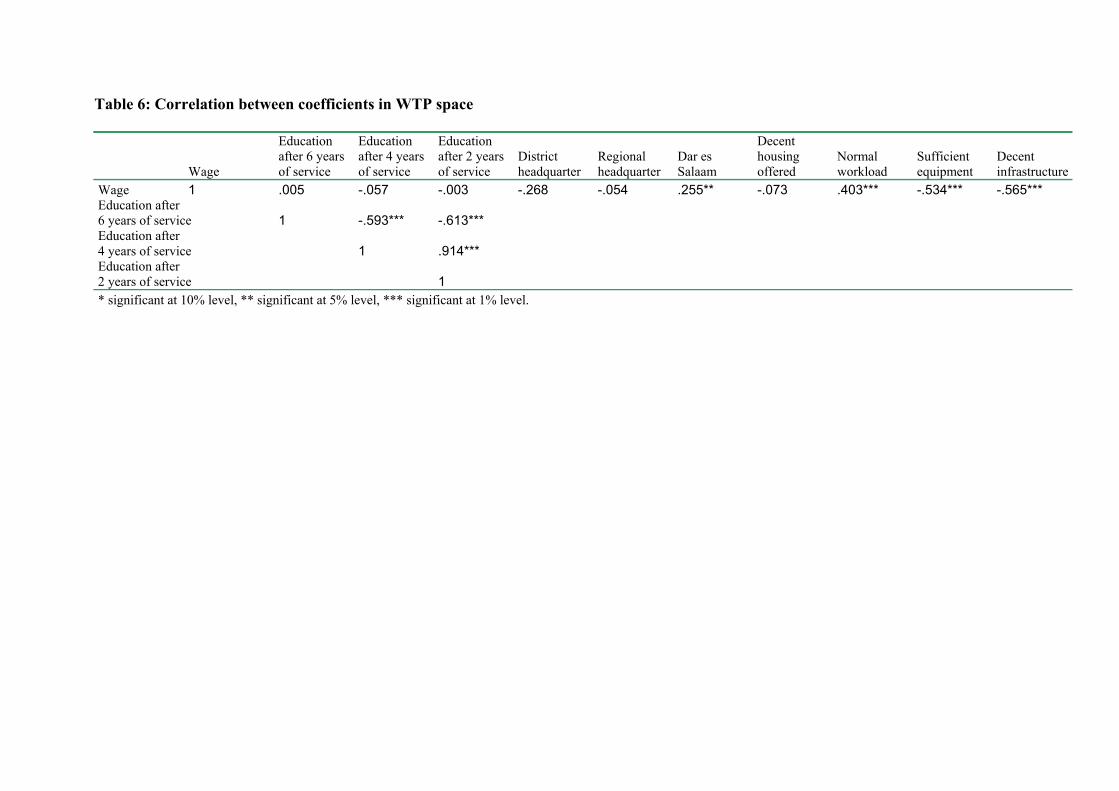
Table 6: Correlation between coefficients in WTP space

Wage






Dar es Salaam


Normal workload



Wage 1 .005 -.057 -.003 -.268 -.054 .255** -.073 .403*** -.534*** -.565*** Education after 6 years of service 1 -.593*** -.613*** Education after 4 years of service 1 .914*** Education after 2 years of service 1 * significant at 10% level, ** significant at 5% level, *** significant at 1% level.

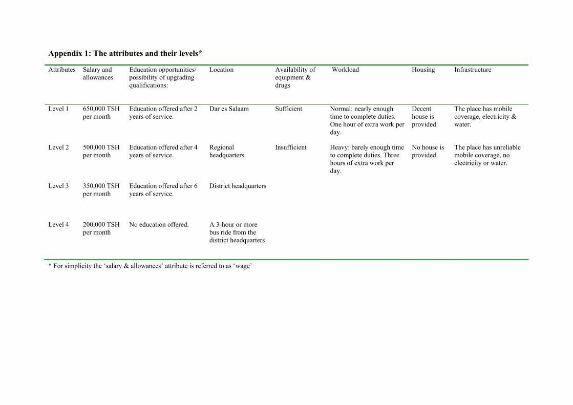
Appendix 1: The attributes and their levels*

Attributes Salary and allowances

Education opportunities/ possibility of upgrading qualifications:

Location Availability of equipment & drugs

Workload Housing Infrastructure

Level 1 650,000 TSH per month

Education offered after 2 years of service.

Dar es Salaam Sufficient Normal: nearly enough time to complete duties. One hour of extra work per day.

Decent house is provided.

The place has mobile coverage, electricity & water.



Regional headquarters

Insufficient Heavy: barely enough time to complete duties. Three hours of extra work per day.

No house is provided.

The place has unreliable mobile coverage, no electricity or water.



District headquarters


No education offered. A 3-hour or more bus ride from the district headquarters

* For simplicity the ‘salary & allowances’ attribute is referred to as ‘wage’

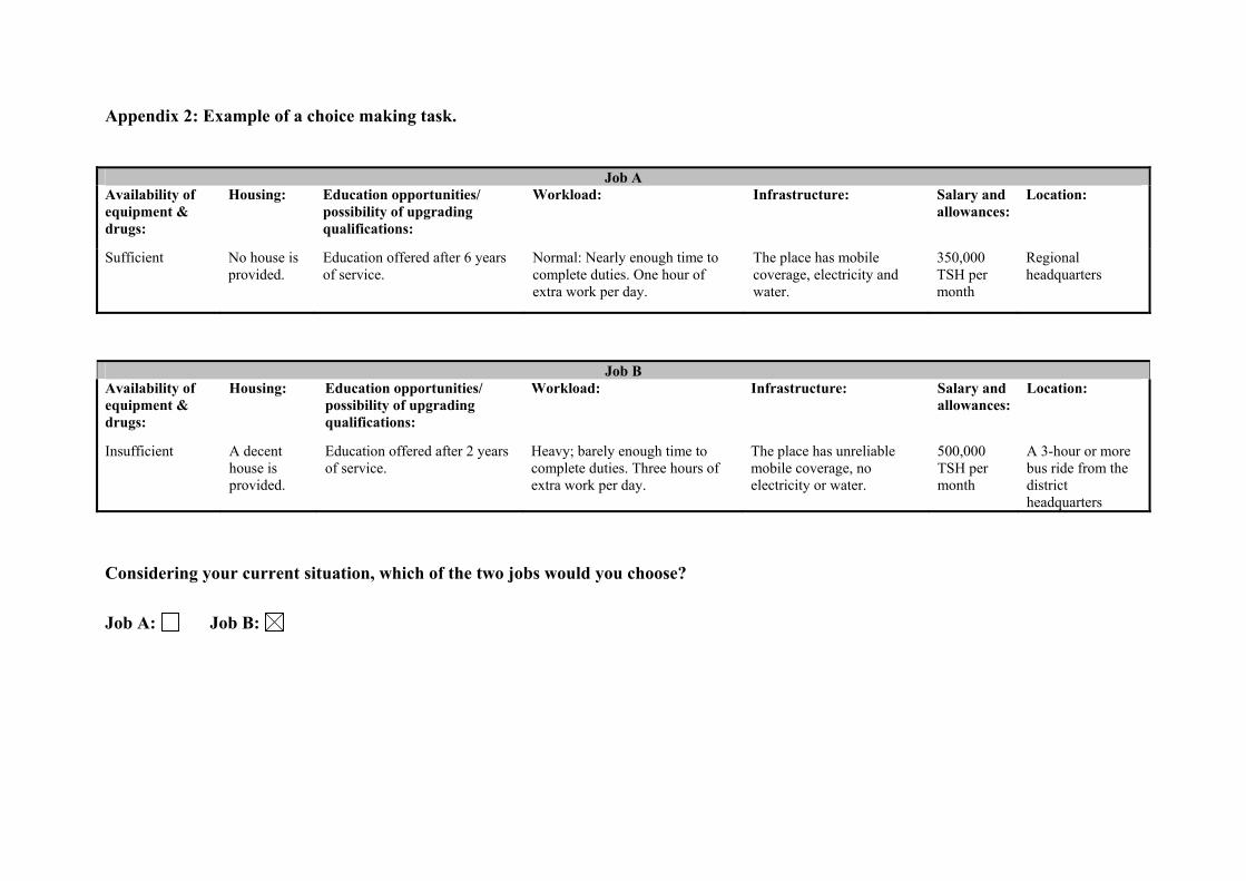
Appendix 2: Example of a choice making task.

Job A Availability of equipment & drugs:

Housing: Education opportunities/ possibility of upgrading qualifications:

Workload: Infrastructure: Salary and allowances:

Location:

Sufficient No house is provided.


Normal: Nearly enough time to complete duties. One hour of extra work per day.

The place has mobile coverage, electricity and water.

350,000 TSH per month

Regional headquarters

Job B Availability of equipment & drugs:

Housing: Education opportunities/ possibility of upgrading qualifications:

Workload: Infrastructure: Salary and allowances:

Location:

Insufficient A decent house is provided.


Heavy; barely enough time to complete duties. Three hours of extra work per day.

The place has unreliable mobile coverage, no electricity or water.

500,000 TSH per month

A 3-hour or more bus ride from the district headquarters

Considering your current situation, which of the two jobs would you choose?

Job A: Job B:

mixed logit estimation of willingness to pay … logit estimation of willingness to pay...

Documents