European Journal of Operational Research 239 (2014) 636–643

Contents lists available at ScienceDirect

European Journal of Operational Research

journal homepage: www.elsevier .com/locate /e jor

Discrete Optimization

Minmax regret 1-facility location on uncertain path networks

http://dx.doi.org/10.1016/j.ejor.2014.06.0260377-2217/� 2014 Elsevier B.V. All rights reserved.

⇑ Tel.: +1 435 797 2416; fax: +14357973265.E-mail address: haitao.wang@usu.edu

Haitao Wang ⇑Department of Computer Science, Utah State University, Logan, UT 84322, USA

a r t i c l e i n f o a b s t r a c t

Article history:Received 29 November 2013Accepted 19 June 2014Available online 28 June 2014

Keywords:AlgorithmsPath networksUncertaintyFacility locationMinmax regret

Let P be an undirected path graph of n vertices. Each edge of P has a positive length and a constant capac-ity. Every vertex has a nonnegative supply, which is an unknown value but is known to be in a giveninterval. The goal is to find a point on P to build a facility and move all vertex supplies to the facility suchthat the maximum regret is minimized. The previous best algorithm solves the problem in Oðn log2nÞ timeand Oðn log nÞ space. In this paper, we present an Oðn log nÞ time and OðnÞ space algorithm, and ourapproach is based on new observations and algorithmic techniques.

� 2014 Elsevier B.V. All rights reserved.

1. Introduction

Facility location problems on networks have received consider-able attention over a few decades. The problems are normally con-cerned with networks where the information (e.g., the vertex andthe edge weights) are known precisely. However, data in practiceoften involve uncertainty and may change with the time. Recentlyfacility locations problems in uncertain environments have beenstudied, e.g., Averbakh and Bereg (2005), Averbakh and Berman(1997, 2000a, 2000b, 2003), Bhattacharya and Kameda (2012),Bhattacharya, Kameda, and Song (2012a, 2012b), Chen and Lin(1998), Cheng et al. (2013), Conde (2007, 2008), Kouvelis and Yu(1997), Puerto, Rodríguez-Chía, and Tamir (2009) and Yu, Lin,and Wang (2008). One approach that is often used to model theuncertainty is the worst-case analysis in which one is looking fora solution that performs reasonably well for all possible scenarios(where a scenario is a specific realization of all uncertain parame-ters of the problem). There are many optimization criteria in theworst-case analysis. In particular, the minmax regret optimizationaims at obtaining a solution that minimizes the maximum devia-tion, over all possible scenarios, between the value of the solutionand the optimal value of the corresponding scenario, e.g., Averbakhand Berman (1997, 2000b), Bhattacharya and Kameda (2012),Bhattacharya et al. (2012a, 2012b), Cheng et al. (2013), Kouvelisand Yu (1997) and Yu et al. (2008). In other words, the minmaxregret optimization seeks to minimize the worst-case loss in theobjective function value that may occur because the solution ischosen without knowing which scenario will take place.

In this paper, we consider the minmax regret 1-facility locationproblem on uncertain path networks where the vertex weights areuncertain. The problem was proposed recently by Cheng et al.(2013) and an Oðnlog2nÞ time and Oðn log nÞ space algorithm wasgiven in Cheng et al. (2013). By discovering more observations,we present an Oðn log nÞ time and OðnÞ space algorithm in thispaper. Shortly after the preliminary version of this paper appearedin Wang (2013), Cheng et al.’s algorithm (Cheng et al., 2013) wasindependently improved to Oðn log nÞ time and Oðn log nÞ space intheir journal paper (Higashikawa et al., 2014).

As discussed in Cheng et al. (2013), the problem is motivated byan earthquake evacuation problem due to the Tohoku-PacificOcean Earthquake that happened in Japan on March 11th, 2011.For example, suppose we have a highway that connects many citiesand we want to find a location on the highway to build an evacu-ation facility such that when earthquake happens we can evacuatepeople in all these cities to the facility as soon as possible. Thenumber of people in each city is uncertain due to different timeperiods (e.g., weekdays, weekends, days, nights, holidays). Weformally introduce the problem below, and some notations areborrowed from Cheng et al. (2013).

1.1. Problem definitions

Let P ¼ ðV ; EÞ be a path graph, with the vertex setV ¼ fv1; . . . ;vng and the edge set E ¼ fe1; . . . ; en�1g, such that ei

connects v i and v iþ1 for each 1 6 i 6 n� 1. Each edge e 2 E has apositive weight lðeÞ. Each vertex v i 2 V has a weight wi (e.g., thenumber of evacuees), which is unknown but is known in a giveninterval w�i ;w

þi

� �with 0 6 w�i 6 wþi . Let c be a constant represent-

ing the capacity of each edge, which is the maximum number of

H. Wang / European Journal of Operational Research 239 (2014) 636–643 637

evacuees passing any point in any unit time. Let s be a positiveconstant representing the time required for traversing a unit dis-tance of every evacuee. Let R be the Cartesian product of all inter-vals ½w�i ;wþi � for 1 6 i 6 n. Every element s 2 R is called a scenariothat is a feasible assignment of weights to the vertices of P. For anyscenario s 2 R, for each 1 6 i 6 n, we denote by wiðsÞ the weight ofthe vertex v i in the scenario s, and w�i 6 wiðsÞ 6 wþi .

As in Cheng et al. (2013), we embed the path P on a real line L(e.g., the x-axis) such that each vertex v i 2 V is associated with thecoordinate xi ¼ x1 þ

Pi�1j¼1lðejÞ for each 2 6 i 6 n. For each point

x 2 L, with a little abuse of notation, we also use x to denote thecoordinate of the point. We use P to denote the set of points x onL with x1 6 x 6 xn. For any point x 2 P, let PLðxÞ ¼ ft 2 P j t < xgand PRðxÞ ¼ ft 2 P j t > xg. Suppose we build a facility at a locationx 2 P. Consider any scenario s 2 R. We use TLðx; sÞ to denote theminimum time for the evacuees on PLðxÞ to move to x; similarly,let TRðx; sÞ denote the minimum time for the evacuees on PRðxÞ tomove to x. Note that if x is at a vertex v i 2 V , then we assumethe evacuees at v i can complete evacuation in no time. As dis-cussed in Cheng et al. (2013), by Kamiyama, Katoh, and Takizawa(2006), TLðx; sÞ and TRðx; sÞ can be expressed as follows.

TLðx; sÞ ¼ maxv i2PLðxÞ

ðx� xiÞ � sþ1c�Xi

j¼1

wjðsÞ& ’

� 1

( );

TRðx; sÞ ¼ maxv i2PRðxÞ

ðxi � xÞ � sþ 1c�Xn

j¼i

wjðsÞ& ’

� 1

( ):

Note that if PLðxÞ ¼ ;; TLðx; sÞ ¼ 0, and if PRðxÞ ¼ ;; TRðx; sÞ ¼ 0.As in Cheng et al. (2013) and Higashikawa et al. (2014), in this

paper we consider the case where c ¼ 1. We should point out thatCheng et al. (2013) claimed that any algorithm works for c ¼ 1 canalso work for any other values of c (our preliminary version (Wang,2013) cited their claim). However, it was found that the claim wasnot correct (Higashikawa et al., 2014), and therefore, their algo-rithms (Cheng et al., 2013; Higashikawa et al., 2014) only workfor the case c ¼ 1 and so does the algorithm in this paper.

But we can ignore the �1 from the above formulas whendesigning the algorithm. Hence, as in Cheng et al. (2013), we sim-ply use the following definitions for TLðx; sÞ and TRðx; sÞ.

TLðx; sÞ ¼ maxv i2PLðxÞ

ðx� xiÞ � sþXi

j¼1

wjðsÞ( )

;

TRðx; sÞ ¼ maxv i2PRðxÞ

ðxi � xÞ � sþXn

j¼i

wjðsÞ( )

:

As in Cheng et al. (2013), for convenience of discussion, for each1 6 i 6 n, we define a function f i

Lðx; sÞ on x > xi and a functionf iRðs; xÞ on x < xi as follows.

f iLðx; sÞ ¼ ðx� xiÞ � sþ

Xi

j¼1

wjðsÞ;

f iRðx; sÞ ¼ ðxi � xÞ � sþ

Xn

j¼i

wjðsÞ:

Hence, we have TLðx; sÞ ¼maxv i2PLðxÞfiLðx; sÞ and TRðx; sÞ ¼

maxv i2PRðxÞfiRðx; sÞ.

Let Tðx; sÞ denote the minimum time for all evacuees on P tomove to x. Thus, Tðx; sÞ ¼maxfTLðx; sÞ; TRðx; sÞg. Denote by xoptðsÞa point on P such that Tðx; sÞ is minimized when x ¼ xoptðsÞ, andone may consider xoptðsÞ as an optimal location for the scenario s.For any point x on L, let Rðx; sÞ ¼ Tðx; sÞ � TðxoptðsÞ; sÞ, and we callRðx; sÞ the regret of x in the scenario s. Intuitively, Rðx; sÞ is theregret (i.e., the opportunity loss) caused by choosing the locationx instead of the optimal location xoptðsÞ. Finally, the maximum regret

of x is defined as RmaxðxÞ ¼maxs2RRðx; sÞ. In other words, RmaxðxÞ isthe worst-case opportunity loss for choosing the location x.

Our minmax regret problem is to choose a location x on L suchthat the maximum regret RmaxðxÞ is minimized, and the minimizedRmaxðxÞ is called the minmax regret.

1.2. Our approach

In this paper we present an algorithm of Oðn log nÞ time andOðnÞ space for the problem, which improves the Oðnlog2nÞ timeand Oðn log nÞ space algorithm (Cheng et al., 2013).

Our algorithm makes use of the critical observation given inCheng et al. (2013) that there are a set S of 2n scenarios such thatfor any point x on L, the ‘‘worst-case’’ scenario for RmaxðxÞ must bein S. This implies that instead of considering the infinitely manyscenarios of R for computing RmaxðxÞ, we only need to considerthe scenarios in S. The algorithm has two main steps. The first stepis to compute the optimal positions for all scenarios in S. AnOðnlog2nÞ time algorithm is given in Cheng et al. (2013) for thestep. By finding new properties on the optimal solutions of thesescenarios, we are able to compute all optimal solutions inOðn log nÞ time by an even simpler algorithm. The second step isto compute the minmax regret. This step also takes Oðnlog2nÞ timein Cheng et al. (2013). Our algorithm runs in Oðn log nÞ time andOðnÞ space. The high level scheme of our approach is binary search,whose efficiency hinges on solving the following sub-problem inlinear time: Given any point x on L, compute the values TLðx; sÞand TRðx; sÞ for all scenarios s 2 S. A straightforward method cancompute TLðx; sÞ and TRðx; sÞ in OðnÞ time for each scenario s, andthus solves the sub-problem in Oðn2Þ time. By discovering someinteresting observations, we present an OðnÞ time algorithm forthe sub-problem. It should be noted that our algorithm itself isvery simple but it is more challenging to observe the crucialproperties behind the scene.

In the following, we discuss some basic observations inSection 2. In Section 3, we compute the optimal locations for allscenarios in S. Section 4 computes the minmax regret. Section 5concludes the paper and discusses some possible future work.

2. Preliminaries

We discuss some observations that will be useful for our algo-rithm. Most of these observations have been discovered in Chenget al. (2013) and we sketch them in this section for completenessof this paper.

Our goal is to find a location x to minimize the maximum regretRmaxðxÞ ¼maxs2RRðx; sÞ. Consider any point x on P and any scenarios 2 R. To compute Rðx; sÞ, we need to known xoptðsÞ first. Recall thatxoptðsÞ is the value of x such that Tðx; sÞ ¼maxfTLðx; sÞ; TRðx; sÞg isminimized when x ¼ xoptðsÞ. To determine xoptðsÞ, we discuss someproperties of TLðx; sÞ and TRðx; sÞ.

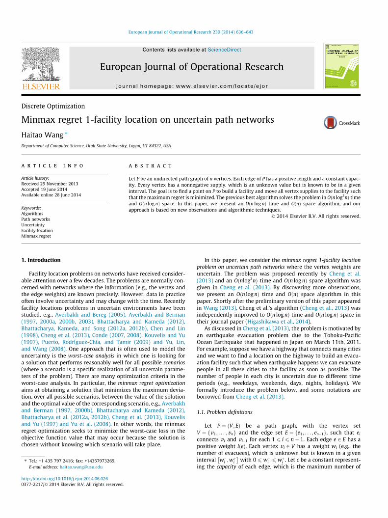
Recall that TLðx; sÞ ¼ maxv i2PLðxÞfiLðx; sÞ. For each 1 6 i 6 n, the

function f iLðx; sÞ defines in the plane an open half-line of slope s with

(but excluding) the (left) endpoint ðxi;Pi

j¼1wjðsÞÞ (e.g., see Fig. 1).TLðx; sÞ is the upper envelope of the n half-lines defined by the func-tions f i

Lðx; sÞ for i ¼ 1; . . . ;n. Since s > 0, TLðx; sÞ is a strictly increas-ing function of x (e.g., see Fig. 1). Similarly, each f i

Rðx; sÞ defines anopen half-line of slope �s with (but excluding) the (right) endpointðxi;Pn

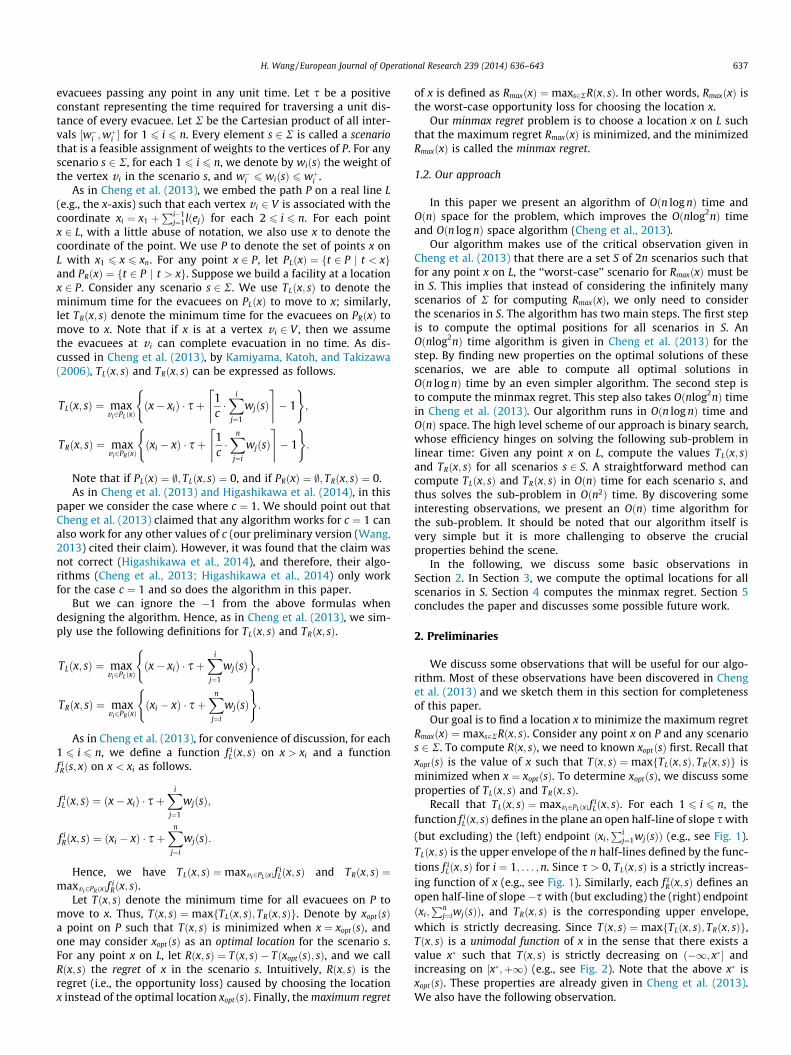
j¼iwjðsÞÞ, and TRðx; sÞ is the corresponding upper envelope,which is strictly decreasing. Since Tðx; sÞ ¼maxfTLðx; sÞ; TRðx; sÞg,Tðx; sÞ is a unimodal function of x in the sense that there exists avalue x� such that Tðx; sÞ is strictly decreasing on ð�1; x�� andincreasing on ½x�;þ1Þ (e.g., see Fig. 2). Note that the above x� isxoptðsÞ. These properties are already given in Cheng et al. (2013).We also have the following observation.

x1 xi

fL1(x,s)

x

fL(x,s)i

Fig. 1. Illustrating the functions f iLðx; sÞ. TLðx; sÞ is the upper envelope of them,

shown with red color. (For interpretation of the references to color in this figurelegend, the reader is referred to the web version of this article.)

638 H. Wang / European Journal of Operational Research 239 (2014) 636–643

Observation 1. For any scenario s 2 R, Tðx; sÞ is the upper envelopeof the functions f i

Lðx; sÞ and f iRðx; sÞ for i ¼ 1; . . . ;n.

For any point x, to compute the maximum regret RmaxðxÞ, astraightforward approach is to enumerate all scenarios in R tocompute Rðx; sÞ for every scenario s 2 R. However, since there areinfinitely many scenarios in R, the approach does not work. Below,we use a difference approach.

A scenario s is the worst-case scenario for the location x ifRmaxðxÞ ¼ Rðx; sÞ, and we denote it by sðxÞ. Clearly, if we knowsðxÞ, then we can compute RmaxðxÞ ¼ Rðx; sðxÞÞ. Cheng et al. (2013)provided a way to determine a set S of at most 2n scenarios suchthat sðxÞ must be in S for any x, as follows.

For each 1 6 i 6 n, let siL be the scenario where the weight wjðsi

LÞof the vertex v j is wþj for each j with 1 6 j 6 i, and wjðsi

LÞ ¼ w�j foreach j with iþ 1 6 j 6 n if i < n. Symmetrically, for each 1 6 i 6 n,let si

R be the scenario where wj siR

� �¼ w�j for each j with 1 6 j 6 i,

and wjðsiRÞ ¼ wþj for each j with iþ 1 6 j 6 n if i < n. Let

SL ¼ siL j 1 6 i 6 n

� �and SR ¼ fsi

R j 1 6 i 6 ng. Let S ¼ SL [ SR. Thefollowing lemma has been proved in Cheng et al. (2013).

Lemma 1 Cheng et al. (2013). For any point x on L, there exists aworst-case scenario for x in S.

In light of Lemma 1, we have RmaxðxÞ ¼maxs2SRðx; sÞ. Hence, tocompute RmaxðxÞ, instead of considering all scenarios of R, we onlyneed to consider the 2n scenarios in S. For each s 2 S, to computeRðx; sÞ, we need to know the optimal location xoptðsÞ. Cheng et al.(2013) presented an Oðnlog2nÞ time algorithm for computingxoptðsÞ for all scenarios s 2 S, and in Section 3 we describe anOðn log nÞ time algorithm.

3. Computing the optimal solutions for the scenarios of S

In this section, we present an Oðn log nÞ time and OðnÞ spacealgorithm for computing xoptðsÞ for all scenarios s 2 S, whichimproves the Oðnlog2nÞ time algorithm in Cheng et al. (2013).

x1xnx*=xopt(s)

x

Fig. 2. Illustrating the function Tðx; sÞ shown with thick segments and the optimallocation xoptðsÞ.

Our improvement is due in a large part to certain monotonicityproperties of the values xoptðsÞ given in Lemma 2.

Lemma 2. For any two scenarios siL and siþ1

L of SL with 1 6 i 6 n� 1,if xiþ1 6 xopt si

L

� �, then xiþ1 6 xopt siþ1

L

� �6 xopt si

L

� �; otherwise,

xopt siL

� �6 xopt siþ1

L

� �6 xiþ1.

Proof. We only prove the case where xiþ1 6 xopt siL

� �since the proof

for the other case where xiþ1 > xopt siL

� �is very similar.

According to the definitions of the two scenarios siL and siþ1

L , foreach vertex v j, if j – iþ 1, the weights of v j in the two scenarios are

the same, but for the vertex v iþ1, wiþ1 siL

� �¼ w�iþ1 and wiþ1 siþ1

L

� �¼

wþiþ1. By Corollary 1 in Cheng et al. (2013), xiþ1 6 xopt siþ1L

� �holds.

Below, we prove xopt siþ1L

� �6 xopt si

L

� �. To this end, it is sufficient to

show that TL x; siþ1L

� �> TR x; siþ1

L

� �for any x > xopt si

L

� �. The details

are given below.Consider any value x > xopt si

L

� �. Since TLðx; sÞ is strictly increas-

ing and TRðx; sÞ is strictly decreasing for any scenario s, according tothe definition of xopt si

L

� �, we have TL x; si

L

� �> TR x; si

L

� �.

According to the definitions of siL and siþ1

L , f jL t; siþ1

L

� �P f j

Lðt; siLÞ

for any j P iþ 1 and any t > xj (more precisely, f jL t; siþ1

L

� �¼

f jLðt; si

LÞ þwþiþ1 �w�iþ1), and f jL t; siþ1

L

� �¼ f j

Lðt; siLÞ for any j 6 i and

any t > xj (e.g., see Fig. 3). Due to x > xopt siL

� �P xiþ1, we obtain

TL x; siþ1L

� �P TL x; si

L

� �.

Similarly, f jR t; siþ1

L

� �P f j

Rðt; siLÞ for any j 6 iþ 1 and any t < xj, and

f jR t; siþ1

L

� �¼ f j

Rðt; siLÞ for any j P iþ 2 and any t < xj (e.g., see Fig. 3).

Since x > xopt siL

� �P xiþ1, none of the functions f j

R t; siþ1L

� �for j 6 iþ 1

is defined on t ¼ x. Therefore, we obtain TR x; siþ1L

� �¼ TR x; si

L

� �.

The above shows that TL x; siL

� �> TR x; si

L

� �; TL x; siþ1

L

� �P TL x; si

L

� �,

and TR x; siþ1L

� �¼ TR x; si

L

� �. Hence, we conclude that

TL x; siþ1L

� �> TR x; siþ1

L

� �. h

Lemma 2 implies the following monotonicity property ofxopt si

L

� �. Suppose initially x2 6 xopt s1

L

� �; as the index i increases,

xopt siL

� �moves monotonically ‘‘backward’’ to the left until at some

moment xiþ1 > xopt siL

� �happens, after which xopt si

L

� �moves mono-

tonically ‘‘forward’’ to the right. This monotonicity property turnsout to be quite useful to our algorithm.

Similarly, we have the following lemma for SR, which implies amonotonicity property of xoptðsi

RÞ (the indices are considered fromright to left).

Lemma 3. For any two scenarios siR and siþ1

R of SR with 1 6 i 6 n� 1,if xi 6 xopt siþ1

R

� �, then xi P xopt si

R

� �P xopt siþ1

R

� �; otherwise,

xopt siþ1R

� �P xopt si

R

� �P xi.

Proof. The proof is symmetric to that for Lemma 2 by consideringthe indices from right to left, and we omit the details. h

xi xi+1

sLix )(opt

sLi+1xopt( )

x

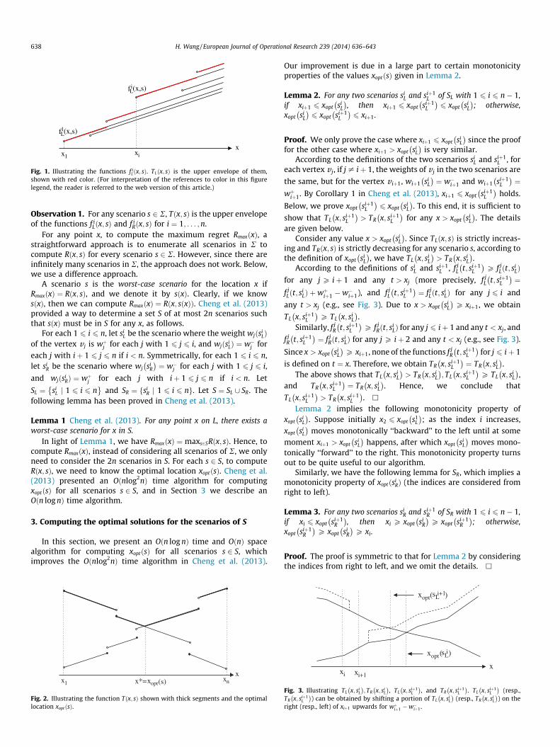
Fig. 3. Illustrating TL x; siL

� �; TR x; si

L

� �, TL x; siþ1

L

� �, and TR x; siþ1

L

� �. TL x; siþ1

L

� �(resp.,

TR x; siþ1L

� �) can be obtained by shifting a portion of TL x; si

L

� �(resp., TR x; si

L

� �) on the

right (resp., left) of xiþ1 upwards for wþiþ1 �w�iþ1.

H. Wang / European Journal of Operational Research 239 (2014) 636–643 639

Based on Lemmas 2 and 3, we present our algorithm for com-puting xoptðsÞ for all s 2 S as follows. We first compute xoptðsÞ forall s 2 SL, by using Lemma 2.

Our algorithm will compute xopt siL

� �in the index order

i ¼ 1;2; . . . ;n. We assume we already have a data structure D thatcan compute the values TLðx; sÞ and TRðx; sÞ whenever needed forany x and s 2 SL. Initially, to determine xopt s1

L

� �, we compute the val-

ues TL x; s1L

� �and TR x; s1

L

� �for x ¼ x1; x2; . . . in the (forward) order to

find the smallest index i1 such that TL xi1 ; s1L

� �P TR xi1 ; s

1L

� �. As

discussed in Cheng et al. (2013), xopt s1L

� �2 ½xi1�1; xi1 � and can be

determined in constant time. Next, we compute xopt x2L

� �. Assume

x2 6 xopt x2L

� �. By Lemma 2, x2 6 xopt x2

L

� �6 xoptðx1

L Þ, we only need tosearch the portions of TL x; s2

L

� �and TR x; s2

L

� �for x2 6 x 6 xopt s1

L

� �.

To this end, we compute the values TL x; s2L

� �and TR x; s2

L

� �by using

D for x ¼ xi1 ; xi1�1; . . . in the (backward) order to find the first indexi2 such that TLðxi2 ; s

2L ÞP TRðxi2 ; s

2L Þ and TL xi2�1; s2

L

� �< TR xi2�1; s2

L

� �.

As discussed in Cheng et al. (2013), xopt s2L

� �2 ½xi2�1; xi2 � and can be

determined in constant time.In general, assume xopt sj

L

� has been computed and xjþ1 6

xopt sjL

� . Further, assume xopt sj

L

� is known in the interval ½xij�1; xij �.

To compute xopt sjþ1L

� , by Lemma 2, we have xjþ1 6 xopt sjþ1

L

� 6 xopt sj

L

� . We compute the values TL x; sjþ1

L

� and TR x; sjþ1

L

� by D

for x ¼ xij ; xij�1; . . . in the (backward) order to find the first index

ijþ1 such that TL xijþ1; sjþ1

L

� P TR xijþ1

; sjþ1L

� and TLðxijþ1�1; s

jþ1L Þ

< TRðxijþ1�1; sjþ1L Þ. Again, xopt sjþ1

L

� 2 ½xijþ1�1; xijþ1

� and can be deter-

mined in constant time.We continue the same procedure until the first time we have

computed xopt skL

� �with xopt sk

L

� �< xkþ1 for an index k. We also have

the interval ½xik�1; xik � that contains xopt skL

� �. By Lemma 2,

xopt skL

� �6 xopt skþ1

L

� �6 xkþ1. Hence, to compute xopt skþ1

L

� �, we need

to search the portions of TL x; skþ1L

� �and TR x; skþ1

L

� �for xopt sk

L

� �6 x.

To this end, we compute the values TL x; skþ1L

� �and TR x; skþ1

L

� �by

D for x ¼ xik�1; xik ; . . . in the (forward) order to find the first indexikþ1 such that TL xikþ1

; skþ1L

� �P TR xikþ1

; skþ1L

� �and TL xikþ1�1; skþ1

L

� �<

TR xikþ1�1; skþ1L

� �. Again, xopt skþ1

L

� �2 ½xikþ1�1; xikþ1

� and can be deter-

mined in constant time. Next, we compute xopt skþ2L

� �. We have

the following observation.

Observation 2. xopt skþ1L

� < xkþ2 holds.

Proof. By Lemma 2, we have xopt skL

� �6 xopt skþ1

L

� �6 xkþ1. Due to

xkþ1 < xkþ2, the observation simply follows. h

Due to the above observation, we can compute xopt skþ2L

� �in the

similar way as xopt skþ1L

� �. We continue this procedure to compute

xoptðsjLÞ for j ¼ kþ 2; kþ 3; . . . ;n. Note that similar observation as

Observation 2 always holds (i.e., xoptðsjLÞ < xjþ1 for any j with

kþ 1 6 j 6 n� 1). The algorithm stops when xoptðsnL Þ is computed.

To analyze the running time, suppose any needed values TLðx; sÞand TRðx; sÞ in the above algorithm can be computed in OðTDÞ timeby using the data structure D; then we have the following lemma.

Lemma 4. The values xoptðsÞ for all scenarios s 2 SL can be computedin Oðn � TDÞ time.

Proof. It is sufficient to show that the number of calls to D is OðnÞin the entire algorithm.

We still use k to denote the smallest index with xopt skL

� �< xkþ1.

By the monotonicity property in Lemma 2, xopt siL

� �is moving

monotonically to the left for i ¼ 1;2; . . . ; k, and xopt siL

� �is moving

monotonically to the right for i ¼ kþ 1; kþ 2; . . . ;n. When wecompute xopt si

L

� �for i ¼ 1; . . . ; k, the x values for computing TL x; si

L

� �and TR x; si

L

� �are monotone decreasing. Therefore, when computing

the values xopt siL

� �’s for i ¼ 1; . . . ; k, the total number of calls on D is

OðnÞ. Analogously, when computing the values xopt siL

� �’s for

i ¼ kþ 1; . . . ;n, the total number of calls on D is also OðnÞ. Thelemma thus follows. h

It remains to design the data structure D, which is given in thefollowing lemma.

Lemma 5. In OðnÞ time and OðnÞ space, we can build a data structure Dthat can compute in Oðlog nÞ time (i.e., TD ¼ Oðlog nÞ) any value TLðx; sÞor TRðx; sÞ needed in our algorithm for computing xoptðsÞ for all s 2 SL.

Proof. With Oðn log nÞ time preprocessing, Cheng et al. (2013) pro-pose a data structure that can compute TLðx; sÞ and TRðx; sÞ for any xand s 2 SL in Oðlog nÞ time, by using persistent data structures(Driscoll, Sarnak, Sleator, & Tarjan, 1989). Below, we give a simplesolution with only OðnÞ preprocessing time, without using the per-sistent data structures.

We first discuss an observation on our algorithm that makes thedesign of our data structure easier. In our algorithm for computingxoptðsÞ for all s 2 SL, when we are computing xopt si

L

� �, for any

1 6 i 6 n, we need to compute TL x; siL

� �and TR x; si

L

� �for certain

values of x. After xopt siL

� �is computed, we will never need to

compute TL x; siL

� �and TR x; si

L

� �for the scenario si

L again. Note thatthe corresponding algorithm in Cheng et al. (2013) does not havesuch a property.

Our data structure D has two parts DL and DR. DL is forcomputing TLðx; sÞ and DR is for computing TRðx; sÞ. Below, we onlydiscuss DL since DR is very similar.

DL consists of a sequence of trees DiL for i ¼ 1;2; . . . ;n, where Di

L

is used for computing TL x; siL

� �for any x. Thanks to the observation

discussed above, at any moment during the algorithm, we onlyneed to maintain one tree in the above sequence (in contrast,because the corresponding algorithm in Cheng et al. (2013) doesnot have such a property, they have to maintain all these trees in apersistent data structure). Specifically, initially we construct the

tree D1L . Then, for each 1 6 i 6 n� 1, the tree Diþ1

L is obtained by

updating the tree DiL in Oðlog nÞ time (Di

L is thus destroyed). Below,

we first describe the tree D1L and then show how to update D1

L to

obtain D2L . The tree is similar to that given in Cheng et al. (2013)

(without being made persistent). We briefly discuss it here to makethe paper self-contained.

We first discuss some observations on how to compute TLðx; sÞ.Consider any scenario s and any value x with xj�1 < x 6 xj for

certain j. Recall that the functions f 1L ðx; sÞ; f 2

L ðx; sÞ; . . . ; f j�1L ðx; sÞ are

defined on x while f jLðx; sÞ; f

jþ1L ðx; sÞ; . . . ; f n

L ðx; sÞ are not, andTLðx; sÞ ¼max16t6j�1f t

L ðx; sÞ. Also recall that f tL ðx; sÞ ¼ ðx� xtÞ � sþPt

h¼1whðsÞ. Hence, we can obtain the following TLðx; sÞ ¼ x � sþmax16t6j�1ð

Pth¼1whðsÞ � xt � sÞ.

D1L is a balanced binary search tree in which the leaves of DL

from left to right store the valuesPt

h¼1wh s1L

� �� xt � s for

t ¼ 1;2; . . . ;n. For each 1 6 t 6 n, let at ¼Pt

h¼1wh s1L

� �� xt � s,

which is stored in the t-th leaf. For each node v (either a leaf oran internal node), it also stores a value maxðvÞ, which is equal tothe maximum value stored in the leaves of the subtree rooted at v.

The tree D1L can be easily constructed in OðnÞ time in a bottom-up

manner. Given any value x ¼ xj; TL x; s1L

� �can be computed in

Oðlog nÞ time, as follows. According to our above discussion, wehave TL xj; s1

L

� �¼ xj � sþmax16t6j�1at . With standard techniques, by

640 H. Wang / European Journal of Operational Research 239 (2014) 636–643

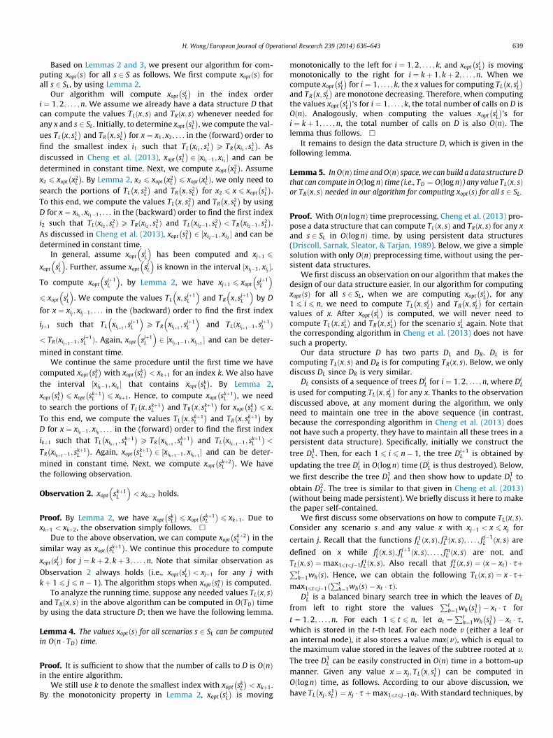
following the path Pj in D1L from the root to the j-th leaf, we find a

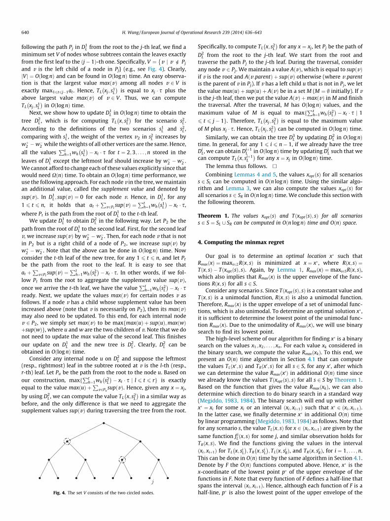
minimum set V of nodes whose subtrees contain the leaves exactlyfrom the first leaf to the ðj� 1Þ-th one. Specifically, V ¼ v j v R Pj

�and v is the left child of a node in Pj} (e.g., see Fig. 4). Clearly,jV j ¼ Oðlog nÞ and can be found in Oðlog nÞ time. An easy observa-tion is that the largest value maxðvÞ among all nodes v 2 V isexactly max16t6j�1at . Hence, TL xj; s1

L

� �is equal to xj � s plus the

above largest value maxðvÞ of v 2 V . Thus, we can computeTL xj; s1

L

� �in Oðlog nÞ time.

Next, we show how to update D1L in Oðlog nÞ time to obtain the

tree D2L , which is for computing TL x; s2

L

� �for the scenario s2

L .

According to the definitions of the two scenarios s1L and s2

L ,comparing with s1

L , the weight of the vertex v2 in s2L increases by

wþ2 �w�2 while the weights of all other vertices are the same. Hence,

all the valuesPt

h¼1wh s1L

� �� xt � s for t ¼ 2;3; . . . ;n stored in the

leaves of D1L except the leftmost leaf should increase by wþ2 �w�2 .

We cannot afford to change each of these values explicitly since thatwould need XðnÞ time. To obtain an Oðlog nÞ time performance, weuse the following approach. For each node v in the tree, we maintainan additional value, called the supplement value and denoted bysupðvÞ. In D1

L ; supðvÞ ¼ 0 for each node v. Hence, in D1L , for any

1 6 t 6 n, it holds that at þP

v2PtsupðvÞ ¼

Pth¼1wh s1

L

� �� xt � s,

where Pt is the path from the root of D1L to the t-th leaf.

We update D1L to obtain D2

L in the following way. Let P2 be the

path from the root of D1L to the second leaf. First, for the second leaf

v, we increase supðvÞ by wþ2 �w�2 . Then, for each node v that is notin P2 but is a right child of a node of P2, we increase supðvÞ bywþ2 �w�2 . Note that the above can be done in Oðlog nÞ time. Nowconsider the t-th leaf of the new tree, for any 1 6 t 6 n, and let Pt

be the path from the root to the leaf. It is easy to see thatat þ

Pv2Pt

supðvÞ ¼Pt

h¼1wh s2L

� �� xt � s. In other words, if we fol-

low Pt from the root to aggregate the supplement value supðvÞ,once we arrive the t-th leaf, we have the value

Pth¼1wh s2

L

� �� xt � s

ready. Next, we update the values maxðvÞ for certain nodes v asfollows. If a node v has a child whose supplement value has beenincreased above (note that v is necessarily on P2), then its maxðvÞmay also need to be updated. To this end, for each internal nodev 2 P2, we simply set maxðvÞ to be maxfmaxðuÞ þ supðuÞ;maxðwÞþsupðwÞg, where u and w are the two children of v. Note that we donot need to update the max value of the second leaf. This finishes

our update on D1L and the new tree is D2

L . Clearly, D2L can be

obtained in Oðlog nÞ time.Consider any internal node u on D2

L and suppose the leftmost(resp., rightmost) leaf in the subtree rooted at v is the l-th (resp.,r-th) leaf. Let Pu be the path from the root to the node u. Based onour construction, maxf

Pth¼1wh s2

L

� �� xt � s j l 6 t 6 rg is exactly

equal to the value maxðuÞ þP

v2PusupðvÞ. Hence, given any x ¼ xj,

by using D2L , we can compute the value TL x; s2

L

� �in a similar way as

before, and the only difference is that we need to aggregate thesupplement values supðvÞ during traversing the tree from the root.

Fig. 4. The set V consists of the two circled nodes.

Specifically, to compute TL x; s2L

� �for any x ¼ xj, let Pj be the path of

D2L from the root to the j-th leaf. We start from the root and

traverse the path Pj to the j-th leaf. During the traversal, considerany node v 2 Pj. We maintain a value AðvÞ, which is equal to supðvÞif v is the root and Aðv:parentÞ þ supðvÞ otherwise (where v :parentis the parent of v in Pj). If v has a left child u that is not in Pj, we letthe value maxðuÞ þ supðuÞ þ AðvÞ be in a set M (M ¼ ; initially). If vis the j-th leaf, then we put the value AðvÞ þmaxðvÞ in M and finishthe traversal. After the traversal, M has Oðlog nÞ values, and themaximum value of M is equal to maxf

Pth¼1wh s2

L

� �� xt � s j 1

6 t 6 j� 1g. Therefore, TL xj; s2L

� �is equal to the maximum value

of M plus xj � s. Hence, TL xj; s2L

� �can be computed in Oðlog nÞ time.

Similarly, we can obtain the tree D3L by updating D2

L in Oðlog nÞtime. In general, for any 1 6 i 6 n� 1, if we already have the treeDi

L, we can obtain Diþ1L in Oðlog nÞ time by updating Di

L such that wecan compute TL x; siþ1

L

� �for any x ¼ xj in Oðlog nÞ time.

The lemma thus follows. h

Combining Lemmas 4 and 5, the values xoptðsÞ for all scenarioss 2 SL can be computed in Oðn log nÞ time. Using the similar algo-rithm and Lemma 3, we can also compute the values xoptðsÞ forall scenarios s 2 SR in Oðn log nÞ time. We conclude this section withthe following theorem.

Theorem 1. The values xoptðsÞ and TðxoptðsÞ; sÞ for all scenarioss 2 S ¼ SL [ SR can be computed in Oðn log nÞ time and OðnÞ space.

4. Computing the minmax regret

Our goal is to determine an optimal location x� such thatRmaxðxÞ ¼maxs2RRðx; sÞ is minimized at x ¼ x�, where Rðx; sÞ ¼Tðx; sÞ � TðxoptðsÞ; sÞ. Again, by Lemma 1, RmaxðxÞ ¼maxs2SRðx; sÞ,which also implies that RmaxðxÞ is the upper envelope of the func-tions Rðx; sÞ for all s 2 S.

Consider any scenario s. Since TðxoptðsÞ; sÞ is a constant value andTðx; sÞ is a unimodal function, Rðx; sÞ is also a unimodal function.Therefore, RmaxðxÞ is the upper envelope of a set of unimodal func-tions, which is also unimodal. To determine an optimal solution x�,it is sufficient to determine the lowest point of the unimodal func-tion RmaxðxÞ. Due to the unimodality of RmaxðxÞ, we will use binarysearch to find its lowest point.

The high-level scheme of our algorithm for finding x� is a binarysearch on the values x1; x2; . . . ; xn. For each value xk considered inthe binary search, we compute the value RmaxðxkÞ. To this end, wepresent an OðnÞ time algorithm in Section 4.1 that can computethe values TLðx0; sÞ and TRðx0; sÞ for all s 2 S, for any x0, after whichwe can determine the value Rmaxðx0Þ in additional OðnÞ time sincewe already know the values TðxoptðsÞ; sÞ for all s 2 S by Theorem 1.Based on the function that gives the value RmaxðxkÞ, we can alsodetermine which direction to do binary search in a standard way(Megiddo, 1983, 1984). The binary search will end up with eitherx� ¼ xi for some xi or an interval ðxi; xiþ1Þ such that x� 2 ðxi; xiþ1Þ.In the latter case, we finally determine x� in additional OðnÞ timeby linear programming (Megiddo, 1983, 1984) as follows. Note thatfor any scenario s, the value TLðx; sÞ for x 2 ðxi; xiþ1Þ are given by the

same function f jLðx; sÞ for some j, and similar observation holds for

TRðx; sÞ. We find the functions giving the values in the intervalðxi; xiþ1Þ for TL x; si

L

� �; TR x; si

L

� �; TLðx; si

RÞ, and TRðx; siRÞ, for i ¼ 1; . . . ;n.

This can be done in OðnÞ time by the same algorithm in Section 4.1.Denote by F the OðnÞ functions computed above. Hence, x� is thex-coordinate of the lowest point p� of the upper envelope of thefunctions in F. Note that every function of F defines a half-line thatspans the interval ðxi; xiþ1Þ. Hence, although each function of F is ahalf-line, p� is also the lowest point of the upper envelope of the

H. Wang / European Journal of Operational Research 239 (2014) 636–643 641

lines that contain the half-lines of F, and thus p� can be computedin OðnÞ time by linear programming (Megiddo, 1983, 1984).

4.1. A linear time algorithm for computing Tðx0; sÞ for all s 2 S

In this section, we present an OðnÞ time algorithm for computingTðx0; sÞ for all s 2 S, for any x0. In other words, our goal is to computethe values TL x0; si

L

� �; TR x0; si

L

� �; TL x0; si

R

� �, and TR x0; si

R

� �, for i ¼ 1; . . . ;n.

We only discuss our algorithm for computing TL x0; siL

� �for

i ¼ 1; . . . ;n since the algorithms for the other three cases are quite

similar. Further, for each 1 6 i 6 n, the function f jL x0; si

L

� �that gives

the value TL x0; siL

� �is also determined by the algorithm.

For any 1 6 i 6 j 6 n, we define aði; jÞ ¼Pj

k¼i wþk �w�k� �

. AfterOðnÞ time preprocessing, given any i and j with 1 6 i 6 j 6 n, wecan obtain the value aði; jÞ in constant time. We omit the prepro-cessing details and below we assume we have done the prepro-cessing. For convenience, we let aði; jÞ ¼ 0 if i > j.

Let x0 be any value with x1 6 x0 6 xn. We first determine theindex i such that xi�1 < x0 6 xi. Thus, for any scenario s, only func-tions f t

L ðx0; sÞ with 1 6 t 6 i� 1 are defined on x ¼ x0, and any func-tion f t

L ðx; sÞ with i 6 t 6 n does not define on x ¼ x0. We computethe value TL x; s1

L

� �, which can be done in OðnÞ time, e.g., by comput-

ing f jL x0; s1

L

� �for each j with 1 6 j 6 i� 1.

Let k be the index such that TL x0; s1L

� �is given by the function

f kL x0; s1

L

� �, e.g., TL x0; s1

L

� �¼ f k

L x0; s1L

� �. Hence, k 6 i� 1. The following

lemma will be useful later.

Lemma 6. Consider a function f tL ðx; sÞ and a scenario sj

L. If

1 6 t; j 6 i� 1, then f tL x0; sj

L

� ¼ f t

L x0; s1L

� �þ að2;mÞ with m ¼

minft; jg. This implies f tL x0; st

L

� �¼ f t

L x0; sjL

� if t 6 j 6 i� 1.

Proof. Consider any t and j with 1 6 t; j 6 i� 1. First of all, sincexi�1 < x0 6 xi; t 6 i� 1, and j 6 i� 1, both functions f t

L x; s1L

� �and

f tL x; sj

L

� are defined on x ¼ x0. Comparing with the scenario s1

L ,

the weight of each vertex vh for 2 6 h 6 j increase by wþh �w�h in

the scenario sjL, and the weights of all other vertices are the same

as before. According to their definitions, we obtain that

f tL x0; s1

L

� �¼ f t

L x0; sjL

� þ að2; tÞ if t 6 j, and f t

L x0; s1L

� �¼ f t

L x0; sjL

� þ

að2; jÞ if t P j. The lemma thus follows. h

With the value TL x0; s1L

� �, the following lemma shows how to

compute TL x0; sjL

� for 2 6 j 6 k.

Lemma 7. If k P 2, for any scenario sjL with 2 6 j 6 k,

TL x0; sjL

� ¼ TL x0; s1

L

� �þ að2; jÞ.

Proof. Assume k P 2. Consider any scenario sjL with 2 6 j 6 k. We

first prove a claim that f kL x0; sj

L

� P f t

L x0; sjL

� for any 1 6 t 6 i� 1.

Due to TL x0; s1L

� �¼ f k

L x0; s1L

� �, it holds that f k

L x0; s1L

� �P f t

L x0; s1L

� �for

any 1 6 t 6 i� 1. Consider any t with 1 6 t 6 i� 1. By Lemma 6,

we have f tL x0; sj

L

� ¼ f t

L x0; s1L

� �þ að2;mÞ, where m ¼minfj; tg. Since

j 6 k, f kL x0; sj

L

� ¼ f k

L x0; s1L

� �þ að2; jÞ holds by Lemma 6. Clearly,

að2; jÞP að2;mÞP 0 due to m 6 j. Therefore, we obtain that

f kL x0; sj

L

� P f t

L x0; sjL

� .

The above claim implies that TL x0; sjL

� ¼ f k

L x0; sjL

� . Since

f kL x0; sj

L

� ¼ f k

L x0; s1L

� �þ að2; jÞ by Lemma 6 and TL x0; s1

L

� �¼

f kL x0; s1

L

� �, the lemma follows. h

Suppose the value TL x0; si�1L

� �has already been computed; the

following lemma shows how to obtain TL x0; sjL

� for i 6 j 6 n.

Lemma 8. For any scenario sjL with i 6 j 6 n, TL x0; sj

L

� ¼ TL x0; si�1

L

� �.

Proof. Recall that for any scenario s only the functions f tL ðx; sÞ with

1 6 t 6 i� 1 are defined on x ¼ x0. Consider any scenario sjL with

i 6 j 6 n. Comparing with si�1L , the weight of each vertex v t in sj

L

increases by wþt �w�t for any i 6 t 6 j, and all other vertex weightsdo not change. Since the above vertex weight increase only affect

the functions f tL x; sj

L

� for t P i and none of these functions is

defined on x ¼ x0, the value TLðx0; sÞ does not change for s ¼ si�1L

and s ¼ sjL. A more formal proof is given below.

Let k0 be the index such that the value TL x0; si�1L

� �is given by

f k0L x0; si�1

L

� �, i.e., TL x0; si�1

L

� �¼ f k0

L x0; si�1L

� �. Note that k0 6 i� 1. Hence,

f k0L x0; si�1

L

� �P f t

L x0; si�1L

� �for any 1 6 t 6 i� 1. In the scenario sj

L, theweights of the vertices v t for 1 6 t 6 i� 1 are the same as those in

si�1L . Therefore, f t

L x0; si�1L

� �¼ f t

L x0; sjL

� for any 1 6 t 6 i� 1. Thus,

f k0L x0; sj

L

� P f t

L x0; sjL

� for any 1 6 t 6 i� 1. We obtain that

TL x0; sjL

� ¼ f k0

L x0; sjL

� . Due to f k0

L x0; sjL

� ¼ f k0

L x0; si�1L

� �and

TL x0; si�1L

� �¼ f k0

L x0; si�1L

� �, we have TL x0; sj

L

� ¼ TL x0; si�1

L

� �. h

Based on the preceding two lemmas, we can easily compute

TL x0; sjL

� for j ¼ 2; . . . ; k in OðnÞ time, and compute TL x0; sj

L

� for

j ¼ i; . . . ;n in OðnÞ time provided that we know the value TL x0; si�1L

� �.

It remains to compute TL x0; stL

� �for t ¼ kþ 1; . . . ; i� 1, for which

we present an OðnÞ time algorithm below. Note that our algorithmitself is simple (see the pseudocode Algorithm 1), but it is not easyto discover the observations behind the scene. Our algorithm willcompute a solution index list K ¼ fk1; k2; . . . ; kdg with the followingproperties:

Property 1. k1 ¼ k and k1 6 k2 6 � � � 6 kd 6 i� 1.

Property 2. For any j with 1 6 j 6 d� 1, fkjL x0; s

kjL

� < f

kjþ1L x0; s

kjþ1L

� and f

kjL x0; s1

L

� �P f

kjþ1L x0; s1

L

� �.

Property 3. For any j with 1 6 j 6 d� 1, for any t with kj 6 t < kjþ1,

either f tL x0; st

L

� �6 f

kjL x0; s

kjL

� or f t

L x0; s1L

� �< f

kjþ1L x0; s1

L

� �. If kd – i� 1,

then for any t with kd 6 t 6 i� 1; f tL x0; st

L

� �6 f kd

L x0; skdL

� .

If we already have such a solution index list K, the lemma belowprovides a way to compute the values TL x0; st

L

� �for kþ 1 6 t 6 i� 1

in OðnÞ time.

Lemma 9. For any scenario stL with kþ 1 6 t 6 i� 1, if kj < t 6 kjþ1

for some 1 6 j 6 d� 1, then TL x0; stL

� �¼max f kj

L x0; stL

� �; f kjþ1

L x0; stL

� �n o;

if kd – i� 1 and kd < t, then TL x0; stL

� �¼ f kd

L x0; stL

� �.

Proof. Consider any scenario stL with kþ 1 6 t 6 i� 1. Recall that

TL x0; stL

� �¼max16m6i�1f m

L x0; stL

� �. To simplify the notation, we use

f mðstÞ to represent f mL x0; st

L

� �. Hence, TL x0; st

L

� �¼max16m6i�1f mðstÞ.

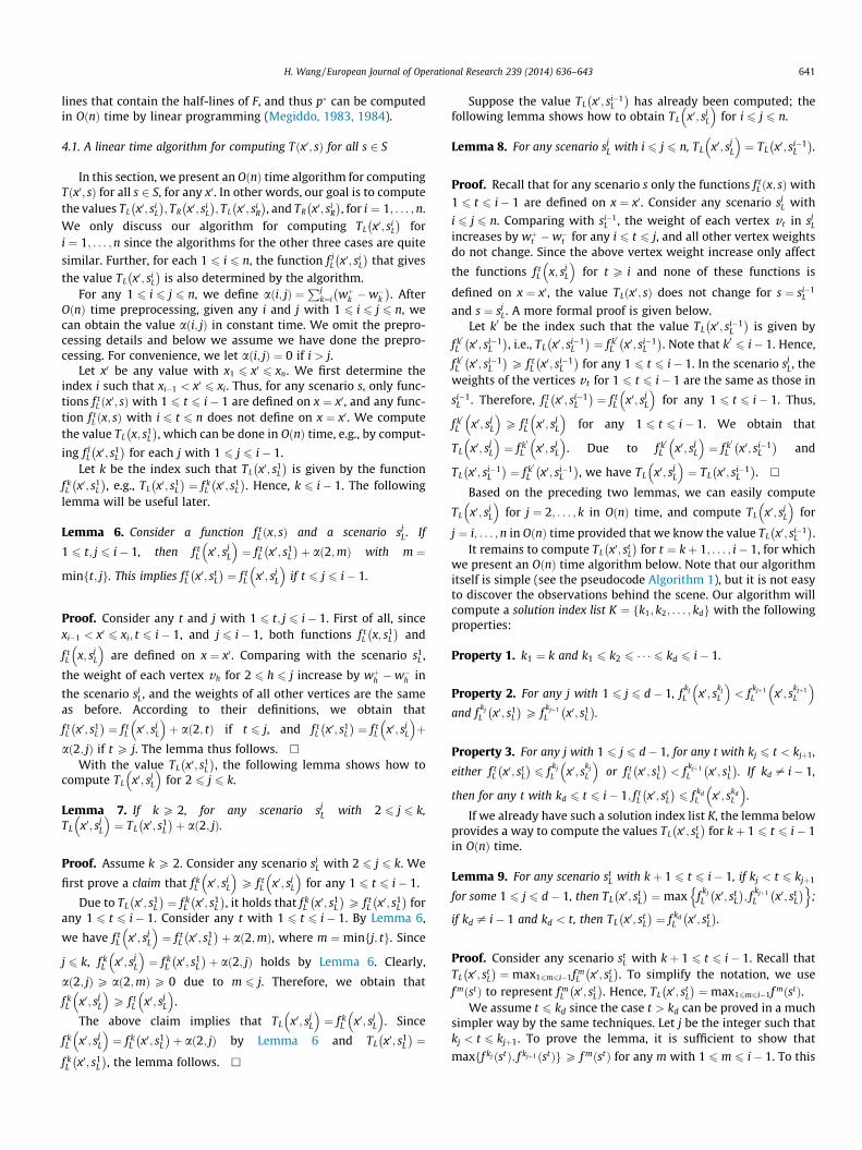
We assume t 6 kd since the case t > kd can be proved in a muchsimpler way by the same techniques. Let j be the integer such thatkj < t 6 kjþ1. To prove the lemma, it is sufficient to show that

maxff kj ðstÞ; f kjþ1 ðstÞgP f mðstÞ for any m with 1 6 m 6 i� 1. To this

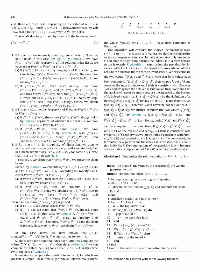
Fig. 5. kh 6 m < khþ1 6 kj < t 6 kjþ1.

642 H. Wang / European Journal of Operational Research 239 (2014) 636–643

end, there are three cases depending on the value of m : 1 6 m< kj; kj 6 m < kjþ1, and kjþ1 6 m 6 i� 1. Below, in each case, we will

show that either f mðstÞ 6 f kj ðstÞ or f mðstÞ 6 f kjþ1 ðstÞ holds.First of all, due to kj < t and by Lemma 6, the following holds

f kj ðstÞ ¼ f kj ðskj Þ: ð1Þ

1. If 1 6 m < kj, we assume kh 6 m < khþ1 for some h < j. Note thatm < t holds in this case. See Fig. 5. By Lemma 6, we havef mðstÞ ¼ f mðsm

L Þ. By Property 3 of the solution index list K, wehave either f mðsmÞ 6 f kh ðskh Þ or f mðs1Þ < f khþ1 ðs1Þ.(a) If f mðsmÞ 6 f kh ðskh Þ, then by Property 2 of K, since h < j, we

can obtain f kh ðskh Þ < f khþ1 ðskhþ1 Þ < � � � < f kj ðskj Þ. Thus, we havef mðstÞ ¼ f mðsmÞ < f kj ðskj Þ. Since f kj ðstÞ ¼ f kj ðskj Þ by Eq. (1), weobtain f mðstÞ < f kj ðstÞ.

(b) If f mðs1Þ < f khþ1 ðs1Þ, then since m < khþ1, we havef mðsmÞ ¼ f mðs1Þ þ að2;mÞ and f khþ1 ðsmÞ ¼ f khþ1 ðs1Þ þ að2;mÞ,and thus f mðsmÞ < f khþ1 ðsmÞ. Note that f khþ1 ðsmÞ 6 f khþ1 ðskhþ1 Þ.Further, due to khþ1 6 kj; f khþ1 ðskhþ1 Þ < f kj ðskj Þ holds by Prop-erty 2 of K. Recall that f mðstÞ ¼ f mðsm

L Þ. Hence, we obtainf mðstÞ ¼ f mðsm

L Þ < f kj ðskj Þ ¼ f kj ðstÞ by Eq. (1).2. If kj 6 m < kjþ1, then by Property 3 of K, either f mðsmÞ 6 f kj ðskj Þ

or f mðs1Þ < f kjþ1 ðs1Þ.(a) If f mðsmÞ 6 f kj ðskj Þ, then since f mðstÞ 6 f mðsmÞ always holds

by Lemma 6 regardless of whether m 6 t or m > t, we havef mðstÞ 6 f kj ðskj Þ ¼ f kj ðstÞ by Eq. (1).

(b) If f mðs1Þ < f kjþ1 ðs1Þ, then since t 6 kjþ1, we havef kjþ1 ðstÞ ¼ f kjþ1 ðs1Þ þ að2; tÞ by Lemma 6. Also, f mðstÞ ¼f mðs1Þ þ að2;minft;mgÞ. Since f mðs1Þ < f kjþ1 ðs1Þ andað2;minft;mgÞ 6 að2; tÞ, we have f mðstÞ 6 f kjþ1 ðstÞ.

3. If kjþ1 6 m 6 i� 1, for simplicity of discussion, we assumem < kd and the case m P kd can be proved very similarly butin a much simpler way. Let kh 6 m < khþ1 for some h > j. Notethat t 6 kjþ1 6 kh 6 m. See Fig. 6.

First of all, we claim that f mðstÞ 6 f kh ðstÞ. We prove the claimbelow.Indeed, by Lemma 6, we can obtain f mðsmÞ ¼ f mðstÞ þ aðt þ 1;mÞand f kh ðskh Þ ¼ f kh ðstÞ þ aðt þ 1; khÞ. According to Property 3 of K,either f mðsmÞ 6 f kh ðskh Þ or f mðs1Þ < f khþ1 ðs1Þ.(a) If f mðsmÞ 6 f kh ðskh Þ, then since aðt þ 1;mÞP aðt þ 1; khÞ (due

to kh 6 m), we obtain f mðstÞ 6 f kh ðstÞ.(b) If f mðs1Þ < f khþ1 ðs1Þ, then by Property 2 of K,

f khþ1 ðs1Þ 6 f kh ðs1Þ. Thus, we obtain f mðs1Þ 6 f kh ðs1Þ. Due tot 6 kh 6 m, we have f mðstÞ ¼ f mðs1Þ þ að2; tÞ andf kh ðstÞ ¼ f kh ðs1Þ þ að2; tÞ. Hence, f mðstÞ 6 f kh ðstÞ holds.

Therefore, the claim f mðstÞ 6 f kh ðstÞ is proved.(a) If jþ 1 ¼ h, the above proves f mðstÞ 6 f kjþ1 ðstÞ.(b) If jþ 1 < h, we claim that f kh ðstÞ 6 f kjþ1 ðstÞ. Indeed, since

t 6 kjþ1 6 kh in this case, by Lemma 6, f kh ðstÞ ¼ f kh ðs1Þþað2; tÞ and f kjþ1 ðstÞ ¼ f kjþ1 ðs1Þ þ að2; tÞ. By Property 2 ofK; f kh ðs1Þ 6 f kjþ1 ðs1Þ. Therefore, f kh ðstÞ 6 f kjþ1 ðstÞ and the claimis proved. Since f mðstÞ 6 f kh ðstÞ, we obtain f mðstÞ 6 f kjþ1 ðstÞ.

In any case above, we have shown that f mðstÞ6 maxff kj ðstÞ; f kjþ1 ðstÞg holds. The lemma thus follows. h

Suppose we have a solution index list K. After we compute thevalues f

kjL x0; s1

L

� �for j ¼ 1; . . . ; d in OðnÞ time, by Lemma 9 we can

compute the values TL x0; stL

� �for all kþ 1 6 t 6 i� 1 in OðnÞ time

(with the help of Lemma 6).It remains to compute the solution index list K, for which we

present a simple linear time algorithm as follows. We assume

the values f tL x0; s1

L

� �for t ¼ 1; . . . ; i� 1 have been computed in

OðnÞ time.Our algorithm will consider the indices incrementally from

t ¼ kþ 1 to t ¼ i� 1. A stack A is maintained during the algorithmto store a sequence of indices. Initially A contains only one indexk, and after the algorithm finishes the index list in A from bottomto top is exactly K. Algorithm 1 summarizes the pseudocode. Foreach t with kþ 1 6 t 6 i� 1, the algorithm proceeds as follows.Let kj be the index on the top of the current stack A. We first compare

the two values f tL x0; s1

L

� �and f

kjL x0; s1

L

� �. Note that both values have

been computed. If f tL x0; s1

L

� �> f

kjL x0; s1

L

� �, then we pop kj out of A and

consider the next top index on A (this is consistent with Property3 of K and we ignore the detailed discussion on this). We claim thatthe stack A will never be empty because the index k is at the bottomof A. Indeed, recall that TL x0; s1

L

� �¼ f k

L x0; s1L

� �by the definition of k.

Hence, f kL x0; s1

L

� �P f m

L x0; s1L

� �for any 1 6 m 6 i� 1, and in particular,

f tL x0; s1

L

� �6 f k

L x0; s1L

� �. Therefore, k will never be popped out of A. If

f tL x0; s1

L

� �6 f

kjL x0; s1

L

� �, we further compare the two values f t

L x0; stL

� �and f

kjL x0; s

kjL

� . By Lemma 6, f t

L x0; stL

� �¼ f t

L x0; s1L

� �þ að2; tÞ and

fkjL x0; s

kjL

� ¼ f

kjL x0; s1

L

� �þ að2; kjÞ. Hence, both f t

L x0; stL

� �and f

kjL x0; s

kjL

� can be computed in constant time. If f t

L x0; stL

� �> f

kjL x0; s

kjL

� , then

we push t on the top of A and set kjþ1 ¼ t (this is consistent withProperty 2 of K); otherwise, we ignore t (this is consistent with Prop-erty 3 of K) and proceed on t þ 1. After t ¼ i� 1 is considered, weterminate the algorithm and the index list in the stack A is our solu-tion index list K. The running time of the algorithm is OðnÞ becauseonce an index is popped out of A it will never be considered again.

Algorithm 1. Computing the solution index list K ¼ fk1; . . . ; kdg

Input: The index k, the value x0, the scenario s1L , the weight

intervals w�i ;wþi

� �Output: The solution index list K ¼ fk1; . . . ; kdg

1 do preprocessing for answering að�; �Þ queries;2 for t 1 to i� 1 do3 determine the function f t

L x; s1L

� �and compute the value

f tL x0; s1

L

� �;

4 end5 initialize a stack A and push k into A;6 for t kþ 1 to i� 1 do7 m the top index in A;8 while f t

L x0; s1L

� �> f m

L x0; s1L

� �do

9 pop m out of A;10 m the top index in A;11 end12 f t

L x0; stL

� � f t

L x0; s1L

� �þ að2; tÞ;

13 f mL x0; sm

L

� � f m

L x0; s1L

� �þ að2;mÞ;

14 if f tL x0; st

L

� �> f m

L x0; smL

� �then

15 push t on the top of A;16 end17 end18 return the index list in A from bottom to top as K;

We conclude this section with the following theorem.

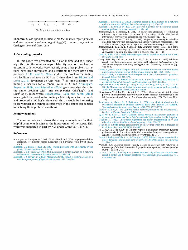
Fig. 6. kj < t 6 kjþ1 6 kh 6 m < khþ1.

H. Wang / European Journal of Operational Research 239 (2014) 636–643 643

Theorem 2. The optimal position x� for the minmax regret problemand the optimal maximum regret Rmaxðx�Þ can be computed inOðn log nÞ time and OðnÞ space.

5. Concluding remarks

In this paper, we presented an Oðn log nÞ time and OðnÞ spacealgorithm for the minmax regret 1-facility location problem onuncertain path networks. Very recently some other problem varia-tions have been introduced and algorithms for them have beenproposed. Li, Xu, and Ni (2014) studied the problem for findingtwo facilities and gave an Oðn3 log nÞ time algorithm. Ni, Xu, andDong (2014) developed an Oðn1þklog1þlog knÞ time algorithm forfinding k facilities for a general value of k, and Arumugam,Augustine, Golin, and Srikanthan (2014) gave two algorithms forthe same problem with time complexities Oðkn2logknÞ andOðkn3 log nÞ, respectively. Higashikawa, Golin, and Katoh (2014)investigated the problem for finding a 1-facility on a tree networkand proposed an Oðnlog2nÞ time algorithm. It would be interestingto see whether the techniques presented in this paper can be usedfor solving these problem variations.

Acknowledgment

The author wishes to thank the anonymous referees for theirhelpful comments leading to the improvement of the paper. Thiswork was supported in part by NSF under Grant CCF-1317143.

References

Arumugam, G. P., Augustine, J., Golin, M., & Srikanthan, P. (2014). A polynomial timealgorithm for minimax-regret evacuation on a dynamic path 1404.5448v1,April.

Averbakh, I., & Bereg, S. (2005). Facility location problems with uncertainty on theplane. Discrete Optimization, 2, 3–34.

Averbakh, I., & Berman, O. (1997). Minimax regret p-center location on a networkwith demand uncertainty. Location Science, 5, 247–254.

Averbakh, I., & Berman, O. (2000a). Algorithms for the robust 1-center problem on atree. European Journal of Operational Research, 123, 292–302.

Averbakh, I., & Berman, O. (2000b). Minmax regret median location on a networkunder uncertainty. INFORMS Journal on Computing, 12, 104–110.

Averbakh, I., & Berman, O. (2003). An improved algorithm for the minmax regretmedian problem on a tree. Networks, 2, 97–103.

Bhattacharya, B., & Kameda, T. (2012). A linear time algorithm for computingminmax regret 1-median on a tree. In Proceedings of the 18th annualinternational conference on computing and combinatorics (pp. 1–12).

Bhattacharya, B., Kameda, T., & Song, Z. (2012). Computing minmax regret 1-medianon a tree network with positive/negative vertex weights. In Proceedings of the23rd international symposium on algorithms and computation (pp. 588–597).

Bhattacharya, B., Kameda, T., & Song, Z. (2012). Minmax regret 1-center on a path/cycle/tree. In Proceedings of the sixth international conference on advancedengineering computing and applications in sciences (pp. 108–113).

Chen, B., & Lin, C.-S. (1998). Minmax-regret robust 1-median location on a tree.Networks, 31, 93–103.

Cheng, S.-W., Higashikawa, Y., Katoh, N., Ni, G., Su, B., & Xu, Y. (2013). Minimaxregret 1-sink location problems in dynamic path networks. In Proceedings of the10th annual conference on theory and applications of models of computation (pp.121–132).

Conde, E. (2007). Minmax regret location allocation problem on a network underuncertainty. European Journal of Operational Research, 179, 1025–1039.

Conde, E. (2008). A note on the minmax regret centdian location on trees. OperationsResearch Letters, 36, 271–275.

Driscoll, J., Sarnak, N., Sleator, D., & Tarjan, R. E. (1989). Making data structurespersistent. Journal of Computer and System Sciences, 38(1), 86–124.

Higashikawa, Y., Auguestine, J., Cheng, S.-W., Golin, M. J., Katoh, N., Ni, G., et al.(2014). Minimax regret 1-sink location problems in dynamic path networks.Theoretical Computer Science. Available online.

Higashikawa, Y., Golin, M. J., & Katoh, N. (2014). Minimax regret sink locationproblem in dynamic tree networks with uniform capacity. In Proceedings of the8th international workshop on algorithms and computation (WALCOM) (pp. 125–137).

Kamiyama, N., Katoh, N., & Takizawa, A. (2006). An efficient algorithm forevacuation problem in dynamic network flows with uniform arc capacity.Transactions on Information and Systems, E89-D(8), 2372–2379.

Kouvelis, P., & Yu, G. (Eds.). (1997). Robust discrete optimization and its applications.Dordrecht: Kluwer Academic Publishers.

Li, H., Xu, Y., & Ni, G. (2014). Minimax regret vertex 2-sink location problem indynamic path networks. Journal of Combinatorial Optimization. Available online.

Megiddo, N. (1983). Linear-time algorithms for linear programming in R3 andrelated problems. SIAM Journal on Computing, 12(4), 759–776.

Megiddo, N. (1984). Linear programming in linear time when the dimension isfixed. Journal of the ACM, 31(1), 114–127.

Ni, G., Xu, Y., & Dong, Y. (2014). Minimax regret k-sink location problem in dynamicpath networks. In Proceedings of the 10th international conference on algorithmicaspects of information and management (AAIM) (pp. 23–31).

Puerto, J., Rodríguez-Chía, A. M., & Tamir, A. (2009). Minimax regret single-facilityordered median location problems on networks. INFORMS Journal on Computing,21, 77–87.

Wang, H. (2013). Minmax regret 1-facility location on uncertain path networks. InProceedings of the 24th international symposium on algorithms and computation(ISAAC) (pp. 733–743).

Yu, H.-I., Lin, T.-C., & Wang, B.-F. (2008). Improved algorithms for the minmax-regret 1-center and 1-median problems. ACM Transactions on Algorithms, 4(3).Article No. 36.